High-performance geodynamics on GPUs using the PETSc CUDA backend (GAUZZ v1.0.0)

GPUs provide much higher memory bandwidth than CPUs. Data-parallel computations with regular memory access patterns exploit the GPU architecture efficiently. To solve the Stokes equations, we apply a preconditioned conjugate-gradient (PCG) method to the Schur complement system. The algorithm is dominated by sparse matrix-vector products, vector inner products, vector updates, and repeated velocity subproblem solves, all of which map onto GPU architectures. We implement the solver in GAUZZ v1.0.0 on GPUs by coupling CUDA-enabled PETSc with FEniCS. PETSc AIJCUSPARSE matrices with CUDA vectors keep operators and field vectors resident in VRAM, which limits CPU-GPU transfers. The P₁ mass matrix, the gradient operator, and the divergence operator are reused in the pressure-correction L₂-projection step. HYPRE BoomerAMG was adopted for preconditioning the velocity-only subproblem. Accuracy and performance are evaluated on a manufactured solution, the SolCx benchmark, the sticky-air benchmark, 2D Rayleigh–Taylor instabilities, 3D thermo-mechanical convection, and a 2D subduction model with nonlinear viscosity. We confirm that the GPU-based implementation reproduces CPU solutions. Performance is quantified by the execution time of the pressure-correction step and by throughput, defined as the number of Stokes degrees of freedom divided by the execution time of one Stokes solve. A single GPU delivers 6–11× the throughput of a 32-core CPU across the Stokes benchmarks. Two GPUs increase the throughput at sufficiently large problem sizes, reaching up to 2.1× the single-GPU throughput. The two-GPU configuration also extends the maximum problem size to 2.5×10⁷ DOFs, beyond the 48 GB VRAM limit of a single GPU.

1 Introduction

Numerical geodynamic modelling has advanced the understanding of plate tectonics and planetary interior physics, including subduction (Yoshida et al., 2012; Keum and So, 2021, 2023; Seong et al., 2026), rifting (Huismans and Beaumont, 2003; Brune et al., 2012; Wolf et al., 2022), folding (Schmalholz, 2008; Do et al., 2023, 2025), plumes (d'Acremont et al., 2003; Gerya et al., 2015; Wang and Li, 2021), and convection (Davies and Gurnis, 1986; Crameri and Tackley, 2015). Over geological time scales spanning millions of years, solid planetary materials flow at low Reynolds numbers due to high viscosity (Gassmöller et al., 2020; Pysklywec and Shahnas, 2003). Thermal heterogeneity and density contrasts drive buoyant flow, governing the heat and material redistribution (Kronbichler et al., 2012; Adams et al., 2023; Regorda et al., 2023; Schools and Smrekar, 2024).

Geodynamic fluid motion is represented by creeping Stokes flow at an infinite Prandtl number (Tan and Gurnis, 2007; Liao and Gerya, 2015). The velocity field obtained from the Stokes equations drives the advection of heat and mantle material, capturing the evolution of planetary interiors from the surface to the core (Schmeling, 2010; Burstedde et al., 2013; Lee et al., 2024). Resolving the coupled, time-dependent Stokes-advection system requires repeated solutions of the Stokes operator. At each time step, the viscosity and density fields are updated. Viscosity often depends nonlinearly on temperature, pressure, composition, and strain rate, which substantially increases the computational cost. Strategies for solving the Stokes equations include direct factorization methods such as LU or LDL^T decomposition (Amestoy et al., 2001; Schenk et al., 2001) and iterative Krylov subspace methods that converge within a specified tolerance (Hestenes and Stiefel, 1952; Saad and Schultz, 1986; Muzhinji et al., 2016).

Efficient solvers for the nonlinear Stokes equations remain essential for numerical simulations of mantle flow with temperature- and strain-rate-dependent viscosity. The strength of mantle and lithospheric rock follows a power-law rheology that links stress to strain-rate, rendering viscosity a function of the strain-rate invariant derived from velocity gradients. Newton and Picard iterations are used to solve for the velocity field. For each nonlinear iteration, the solver linearizes the strongly nonlinear Stokes system and updates viscosity based on the most recent velocity estimate. The iterative procedure repeats until velocity and pressure converge, constituting a principal source of computational expense in geodynamic models due to the tight coupling between viscosity and velocity.

Three-dimensional (3D) geodynamic simulations resolved on a $N\times N\times N$ grid with finite elements P₂×P₁ yield O(N³) degrees of freedom (DOFs). A direct solver requires memory that grows as O(N⁴) (Chen et al., 2018). To overcome memory limitations, Krylov methods such as GMRES or MINRES are commonly used for the full saddle-point Stokes system, while CG is typically applied to symmetric positive-definite sub-blocks (e.g., velocity blocks or Schur complements). The convergence rate of an iterative solver depends critically on the choice of preconditioner. Multigrid preconditioning represents standard practice for simulations at high spatial resolution. Algebraic multigrid (AMG) accelerates convergence by automatically constructing a hierarchy of coarse level representations from the matrix coefficients alone, without requiring an explicit coarse mesh. This property makes AMG particularly suitable for unstructured finite-element discretization.

Many geodynamic problems, such as incompressible viscoelasticity (Zhong et al., 2003; Beuchert and Podladchikov, 2010) and the Stokes equations (Tan and Gurnis, 2007), are formulated as saddle-point problems imposing an incompressibility constraint. Eliminating the velocity unknown from the saddle-point system yields the Schur complement equation for pressure, which can be solved iteratively (Uzawa, 1989; Moresi et al., 1996; Leng and Zhong, 2008). At each iteration, the current pressure p enters the source term, and the algorithm subsequently computes the velocity components $(u,v,w)$ from the velocity-only submatrix. The velocity-only submatrix of the Stokes system is symmetric positive definite. AMG-preconditioned CG or GMRES solves the velocity subproblem efficiently (Clevenger and Heister, 2021). Each pressure-correction iteration requires one such velocity subproblem solve, making it the dominant computational cost. A widely used alternative is to solve the full saddle-point system with block-preconditioned FGMRES, where the Schur complement is approximated by a viscosity-weighted mass matrix or BFBT-type preconditioner (Benzi et al., 2005; May and Moresi, 2008; Rudi et al., 2017). However, even with restart, FGMRES stores substantially more Krylov basis vectors per cycle than the CG-based approach and restart itself may degrade convergence. Additional memory is required to store the Krylov basis vectors generated during each FGMRES restart cycle. In contrast, short-recurrence Krylov methods such as BiCGStab and IDR(s) maintain a fixed storage requirement independent of the iteration number. Clevenger and Heister (2021) used BiCGStab and IDR(s) to solve the full Stokes system in 3D mantle convection simulations. Applying CG to the pressure Schur complement system forms a nested iteration structure. The outer CG iteration updates the pressure, while each Schur-complement evaluation requires an inner linear solve with the velocity stiffness matrix. Despite the nested structure, the outer iteration requires only a fixed, small number of pressure- and velocity-space vectors. The inner velocity solve adds separate Krylov storage. As problem size grows in 3D, where DOFs scale as O(N³), the velocity subproblem solve increasingly dominates the total computation time, and efficient preconditioning becomes essential. Several CPU-based geodynamic community codes have been developed to handle such complex systems, including ASPECT (Kronbichler et al., 2012), Fluidity (Davies et al., 2011), CitcomS (Zhong et al., 2008), FANTOM (Thieulot, 2011), Underworld2 (Mansour et al., 2020), and pTatin3D (May et al., 2015). Such packages have been widely applied to simulate large-scale geodynamic processes, such as continental rifting (Neuharth et al., 2021; Chang and So, 2025; Jang and So, 2026), subduction (Suchoy et al., 2021), and mantle plume dynamics (Xie et al., 2024; Roy et al., 2024). Parallel execution is typically achieved through MPI (Message Passing Interface) libraries such as MPICH and Open MPI (Thakur et al., 2005; Graham et al., 2006). The MPI-based architecture delivers strong scalability, yielding near-linear speedup on thousands of CPU cores (Burstedde et al., 2013).

A GPU integrates thousands of arithmetic units designed for massively parallel computation (Ta et al., 2015). A CPU uses a few complex cores designed for fast sequential computation. The GPU also accesses memory at a higher bandwidth than the CPU, with theoretical peaks of 960 and 153.6 GB s⁻¹ for the NVIDIA RTX 6000 Ada Generation and the Xeon Gold 6338 workstation used in this study, respectively. Sparse matrix–vector products and vector updates dominate the cost of Krylov solvers (May et al., 2015). Both operations perform approximately one multiplication and one addition per value read from memory (Williams et al., 2009). The low ratio of arithmetic to memory traffic, termed arithmetic intensity, makes memory bandwidth, rather than the number of arithmetic units or cores, a strong control on the cost of the two operations. Preconditioning and other solver steps also contribute to the time per Krylov iteration.

To date, GPU-based solutions of the Stokes equations in geodynamic modelling have often used pseudo-transient (PT) methods (Räss et al., 2022), which have also been extended to fluid flow and to elastic, viscoelastic, and hydromechanical problems (Wang et al., 2022; Alkhimenkov and Podladchikov, 2025). PT methods augment the governing equations with pseudo-time derivatives and integrate them explicitly until the residuals are reduced below a prescribed tolerance. In the cited Stokes implementations, the explicit update applies local finite-difference stencils on regular staggered grids, requiring no assembly of global matrices. The matrix-free formulation keeps the memory footprint small, which suits GPUs with limited device memory. The accelerated PT method adds pseudo-time terms that give rise to damped-wave dynamics (Räss et al., 2022). With near-optimal iteration parameters, the iteration count grows approximately linearly, rather than quadratically, with the number of grid cells along one dimension. Räss et al. (2022) demonstrated convergence for viscosity contrasts of up to nine orders of magnitude. Convergence slowed in some of the high-contrast cases. In contrast, GPU implementations of Krylov solvers with algebraic multigrid preconditioning, the standard approach in finite-element geodynamic codes, have received less attention.

PETSc (Portable, Extensible Toolkit for Scientific Computation; Balay et al., 2025) provides a unified interface to Krylov subspace solvers, sparse matrix storage, and external preconditioner packages across both CPU and GPU environments. Among its external interfaces, the HYPRE library and its BoomerAMG algebraic multigrid preconditioner (Falgout et al., 2006) are particularly relevant to geodynamic applications, where viscosity contrasts of 10³–10⁶ render the discretized Stokes system highly ill-conditioned. Since version 3.16 (released in September 2021), PETSc has supported GPU-resident execution of HYPRE preconditioners, enabling the entire Krylov iteration, including matrix–vector products, vector operations, and AMG preconditioning cycles, to remain on the GPU, minimising host–device data transfer. However, in geodynamic modelling, the performance of BoomerAMG on GPUs has not yet been systematically evaluated, and quantitative comparisons between the GPU and CPU environments remain limited.

In this study, we developed a solver for the Stokes system using FEniCS, an open-source finite element platform (Alnæs et al., 2015). The saddle-point system is reduced via the Schur complement, and the resulting pressure equation is solved by a preconditioned conjugate-gradient (PCG) method with the inverse viscosity mass matrix. Both CPU and GPU execution paths are provided. The CPU path links against PETSc 3.15.5, while the GPU path links against PETSc 3.23.2 compiled with CUDA support, storing all matrices and vectors in GPU VRAM using the AIJCUSPARSE and CUDA vector types. To benchmark CPU and GPU performance, we selected a suite of benchmark problems from computational geodynamics, including manufactured solutions, the SolCx viscosity-discontinuity benchmark, sticky-air free-surface tests, 2D Rayleigh–Taylor instabilities, 3D thermo-mechanical convection, and a subduction scenario with nonlinear mantle viscosity. For problems that involve advection, we also evaluated the performance of the advection equation solver. A comparison with block-preconditioned Stokes solvers widely adopted in geodynamic community codes is presented in Sect. 5.4. All experiments were performed on three machines with different performance characteristics. The first workstation used an Intel Xeon Gold 6338 processor (2.00 GHz, 48 MB cache, 32 physical cores and 64 threads). The second workstation used an Intel Xeon w5-2465X processor (3.10 GHz, 33.75 MB cache, 16 physical cores and 32 threads) and an NVIDIA RTX 6000 Ada Generation GPU with 48 GB of memory. The third workstation used the same processor but was paired with two NVIDIA RTX 6000 Ada Generation GPUs, each with 48 GB of memory (96 GB in total). The Xeon Gold 6338 supports eight DDR4-3200 memory channels, six of which are populated in the CPU workstation used here, giving a theoretical memory bandwidth of 153.6 GB s⁻¹. The theoretical bandwidth per NVIDIA RTX 6000 Ada Generation is 960 GB s⁻¹. We measured the sustained bandwidth with a memory benchmark based on the vector update $a=a+s\cdot b$, following the approach of Deakin et al. (2018). The benchmark sustained 824.0 GB s⁻¹ on a single GPU (86 % of the peak) and 113.2 GB s⁻¹ on the 32-core CPU (74 % of the peak) (Table S1 in the Supplement). All CPU execution times reported in this study were measured on the first workstation, with one MPI rank assigned to each physical core. The second and third workstations were used for the single-GPU and two-GPU calculations, respectively. In both GPU systems, the Xeon w5-2465X processor handled matrix assembly, mesh-related operations, and CPU–GPU data management, while the linear solves were executed on the GPU. Unlike previous GPU-based geodynamic studies, which primarily rely on PT formulations, our study directly evaluates the performance of Krylov solvers with algebraic multigrid preconditioning for mixed finite-element Stokes systems on GPUs.

2 Methods

2.1 Governing equations

Lithospheric deformation and mantle flow associated with geodynamic processes are described by the Stokes equations for incompressible viscous creeping flow (Eqs. 1 and 2). We incorporated the thermal (Ra) and compositional (Rb) Rayleigh numbers (Eq. 3) into the buoyancy term (e.g., van Keken et al., 1997; Tan et al., 2011). Equations (1) and (4) assume a general form, with each benchmark activating only the terms required by the physical setting. Thermal-buoyancy cases set Rb=0, while compositional-buoyancy cases set Ra=0 in the absence of a temperature field. The presence of a temperature field determines whether Eq. (4) enters the solution. Each calculation adopts one of the two settings alone, keeping the thermal and compositional drivers separate.

$$\begin{array}{}\text{(1)}& {\displaystyle }\begin{array}{rl}{\displaystyle }\mathrm{\nabla }\cdot \mathit{\tau }-\mathrm{\nabla }p& {\displaystyle }+\left[\mathit{Ra}T-{\sum }_i{\mathit{Rb}}_i{C}_i\right]\widehat{\mathit{z}}=\mathbf{0}\\ {\displaystyle }& {\displaystyle }\text{where }\mathit{\tau }=\mathrm{2}\mathit{\eta }\dot{\mathit{\epsilon }}\text{ and }\dot{\mathit{\epsilon }}={\displaystyle \frac{\mathrm{1}}{\mathrm{2}}}(\mathrm{\nabla }\mathit{u}+(\mathrm{\nabla }\mathit{u}{)}^T)\end{array}\text{(2)}& {\displaystyle }\mathrm{\nabla }\cdot \mathit{u}=\mathrm{0}\text{(3)}& {\displaystyle }\mathit{Ra}={\displaystyle \frac{\mathit{\alpha }{\mathit{\rho }}_{\mathrm{0}}g\mathrm{\Delta }T{h}^{\mathrm{3}}}{\mathit{\kappa }{\mathit{\eta }}_{\mathrm{0}}}}\text{ and }{\mathit{Rb}}_i={\displaystyle \frac{\mathrm{\Delta }{\mathit{\rho }}_{i}g{h}^{\mathrm{3}}}{\mathit{\kappa }{\mathit{\eta }}_{\mathrm{0}}}}\end{array}$$

p, u, τ, η, $\widehat{\mathit{z}}$, and $\dot{\mathit{\epsilon }}$ denote pressure, velocity vector, the deviatoric stress tensor, shear viscosity, the upward unit vector, and the deviatoric strain-rate tensor, respectively. T and C refer to the temperature and composition fields, respectively. κ, η₀, h, and g are thermal diffusivity, reference viscosity, the depth of the domain, and gravitational acceleration, respectively. α, ρ₀, ΔT, and Δρ_i represent the thermal expansivity, reference density, temperature contrast between the bottom and top, and the density contrast of the ith composition relative to ρ₀, respectively. For the Stokes system, we employ two mixed finite-element pairs, the Taylor–Hood element (P₂×P₁) and the MINI element ($P_{\mathrm{1}}^{+}\times P_{\mathrm{1}}$). Both discretizations use the same P₁ pressure space, while the $P_{\mathrm{1}}^{+}$ velocity space enriches P₁ with bubble functions. The pair $P_{\mathrm{1}}^{+}\times P_{\mathrm{1}}$ is commonly referred to as the MINI element in the geodynamics literature (Thieulot and Bangerth, 2025). The MINI element was adopted to reduce the total number of DOFs in high-resolution and 3D simulations. The thermal evolution of the system is governed by the advection-diffusion equation (Eq. 4).

$$\begin{array}{}\text{(4)}& {\displaystyle \frac{\partial T}{\partial t}}+\mathit{u}\cdot \mathrm{\nabla }T=\mathrm{\nabla }\cdot \left(\mathrm{\nabla }T\right)\end{array}$$

The temporal evolution of the multi-composition field depends only on advection through the velocity field. We adopted a level-set method to reduce oscillations and numerical diffusion of the compositional field under advection-dominated conditions (Hillebrand et al., 2014; Wú et al., 2023). The advection of the level-set function ϕ governs the evolution of the composition field (Eq. 5). The level-set function is reinitialized to a signed-distance function satisfying $\left|\mathrm{\nabla }\mathit{\varphi }\right|=\mathrm{1}$ by solving the reinitialization equation (Eq. 6) using second-order ENO spatial discretization, a Godunov Hamiltonian, and RK2 pseudo-time integration.

$$\begin{array}{}\text{(5)}& {\displaystyle \frac{\partial \mathit{\varphi }}{\partial t}}+\mathit{u}\cdot \mathrm{\nabla }\mathit{\varphi }=\mathrm{0}\text{(6)}& {\displaystyle \frac{\partial \mathit{\varphi }}{\partial \mathit{\tau }}}+S\left({\mathit{\varphi }}_{\mathrm{0}}\right)\left(\right|\mathrm{\nabla }\mathit{\varphi }|-\mathrm{1})=\mathrm{0},\text{where}S\left({\mathit{\varphi }}_{\mathrm{0}}\right)={\displaystyle \frac{{\mathit{\varphi }}_{\mathrm{0}}}{\sqrt{{\mathit{\varphi }}_{\mathrm{0}}^{\mathrm{2}}+{\mathit{\epsilon }}^{\mathrm{2}}}}}\end{array}$$

S, ϕ₀, and ε denote the smoothed sign function, the level-set function before reinitialization, and the smoothing parameter, respectively, with $\mathit{\epsilon }=\mathrm{1.5}min(\frac{\mathrm{1}}{N_x},\frac{\mathrm{1}}{N_y})$. N_x and N_y are the numbers of grid cells in the x and y directions, respectively. The level-set function ϕ is a continuous scalar field with the interface defined by ϕ=0. The different material domains are distinguished by ϕ<0 and ϕ≥0. Using the composition field obtained via the level-set functions, density and the logarithm of viscosity were linearly interpolated. To define n compositions, n−1 level-set functions are required. We employed one to four level-set functions (one for Rayleigh–Taylor instability and four for the subduction model).

2.2 Saddle-point problem and Schur complement solver

Discretization of the incompressible Stokes equations yields a 2×2 block saddle-point system (Eq. 7).

$$\begin{array}{}\text{(7)}& \left(\begin{array}{cc}\mathbf{K}& \mathbf{G}\\ {\mathbf{G}}^T& \mathrm{0}\end{array}\right)\left(\begin{array}{c}\mathit{u}\\ \mathit{p}\end{array}\right)=\left(\begin{array}{c}\mathit{f}\\ \mathbf{0}\end{array}\right)\end{array}$$

The velocity stiffness matrix K is symmetric and positive definite (Davies et al., 2011). G and G^T represent the gradient and divergence operators for the pressure and velocity fields, respectively (Silvester and Wathen, 1994; Benzi et al., 2005; May and Moresi, 2008). f denotes the body force vector. In geodynamic applications, the viscosity contrast ranges from 10³ to 10⁶, which leads to an ill-conditioned system and slow convergence of iterative solvers. Furthermore, using a direct solver (e.g., MUMPS) on the full block system causes excessive memory consumption for large-scale problems. Therefore, iterative methods are essential for large-scale problems. One effective approach is to exploit the Schur complement structure of the saddle-point system.

With Schur complement reduction, the Stokes system is transformed into a block upper triangular form (Wathen and Silvester, 1993; Eq. 8).

$$\begin{array}{}\text{(8)}& \left(\begin{array}{cc}\mathbf{K}& \mathbf{G}\\ \mathrm{0}& \mathbf{S}\end{array}\right)\left(\begin{array}{c}\mathit{u}\\ \mathit{p}\end{array}\right)=\left(\begin{array}{c}\mathit{f}\\ \widehat{\mathit{h}}\end{array}\right),\mathbf{S}={\mathbf{G}}^T{\mathbf{K}}^{-\mathrm{1}}\mathbf{G},\widehat{\mathit{h}}={\mathbf{G}}^T{\mathbf{K}}^{-\mathrm{1}}\mathit{f}\end{array}$$

To solve the equivalent system ${\mathbf{G}}^T{\mathbf{K}}^{-\mathrm{1}}\mathbf{G}\mathit{p}={\mathbf{G}}^T{\mathbf{K}}^{-\mathrm{1}}\mathit{f}$, we apply a PCG iteration with the inverse viscosity mass matrix as preconditioner (Eqs. 9–14; Jang et al., 2025).

Initialization:

$$\begin{array}{}\text{(9)}& {\displaystyle }{\mathit{p}}^{\mathrm{0}}=\mathbf{0},\mathbf{K}{\mathit{u}}^{\mathrm{0}}=\mathit{f}-\mathbf{G}{\mathit{p}}^{\mathrm{0}}\left(\text{initial solve}\right)\text{(10)}& {\displaystyle }\begin{array}{rl}{\displaystyle }\langle q^{\mathrm{0}},r\rangle =& {\displaystyle }\langle \mathrm{\nabla }\cdot {\mathit{u}}^{\mathrm{0}},r\rangle ,〈{\displaystyle \frac{\mathrm{1}}{\mathit{\eta }}}{w}^{\mathrm{0}},r〉=\langle q^{\mathrm{0}},r\rangle ,{\mathit{d}}^{\mathrm{0}}=-{\mathit{w}}^{\mathrm{0}}\\ {\displaystyle }& {\displaystyle }\left(\text{initial residual and precond.}\right)\end{array}\end{array}$$

For $k=\mathrm{0},\mathrm{1},\mathrm{2},\mathrm{\dots }$:

$$\begin{array}{}\text{(11)}& {\displaystyle }{\displaystyle }\mathbf{K}{\mathit{h}}^k=\mathbf{G}{\mathit{d}}^k,{\mathit{\alpha }}^k{\displaystyle }={\displaystyle \frac{\langle q^k,w^k\rangle }{\langle \mathrm{\nabla }{d}^k,{\mathit{h}}^k\rangle }}\left(\text{inner solve and step size}\right)\text{(12)}& {\displaystyle }{\displaystyle }{\mathit{p}}^{k+\mathrm{1}}={\mathit{p}}^k+{\mathit{\alpha }}^k{\mathit{d}}^k,{\mathit{u}}^{k+\mathrm{1}}={\mathit{u}}^k{\displaystyle }-{\mathit{\alpha }}^k{\mathit{h}}^k\left(\text{vector update}\right)\text{(13)}& {\displaystyle }\begin{array}{rl}{\displaystyle }\langle q^{k+\mathrm{1}},r\rangle =& {\displaystyle }\langle \mathrm{\nabla }\cdot {\mathit{u}}^{k+\mathrm{1}},r\rangle ,〈{\displaystyle \frac{\mathrm{1}}{\mathit{\eta }}}{w}^{k+\mathrm{1}},r〉=\langle q^{k+\mathrm{1}},r\rangle \\ {\displaystyle }& {\displaystyle }\left(\text{divergence and precond.}\right)\end{array}\text{(14)}& {\displaystyle }{\displaystyle }{\mathit{\beta }}^k={\displaystyle \frac{\langle q^{k+\mathrm{1}},w^{k+\mathrm{1}}\rangle }{\langle q^k,w^k\rangle }},{\mathit{d}}^{k+\mathrm{1}}=-{\mathit{w}}^{k+\mathrm{1}}{\displaystyle }+{\mathit{\beta }}^k{\mathit{d}}^k\left(\text{CG update}\right)\end{array}$$

The pressure is updated along the conjugate direction d^k, while the velocity is updated using the corresponding velocity-space vector h^k. The iteration stops when the divergence error ($\parallel \mathrm{\nabla }\cdot \mathit{u}\parallel /\parallel \mathit{u}\parallel$) of velocity is lower than the divergence tolerance. The algorithm (Eqs. 9–14) requires only a fixed number of vectors in the outer PCG iteration: approximately four in the pressure space (q^k, d^k, p^k, w^k) and two in the velocity space (h^k, u^k). The inner velocity subproblem is solved with GMRES, requiring a separate Krylov basis. However, the symmetric positive definiteness of the velocity stiffness matrix K also permits CG as an alternative inner solver. CG uses a short recurrence with only a few stored vectors, offering a potential reduction in Krylov-vector memory. A further option applies a fixed number of BoomerAMG V-cycles directly as a spectrally equivalent approximation of K⁻¹ within the outer PCG iteration, removing the inner Krylov solver. Outside the velocity subproblem solve (Eq. 11), the remaining operations include vector inner products, scalar–vector multiplications, and vector additions (Eqs. 12 and 14). Memory bandwidth limits the speed of the three operations, which map directly onto GPU architectures. The dominant cost per iteration is the AMG-preconditioned GMRES solve of the velocity subproblem Kh^k=Gd^k (Eq. 11), which involves repeated sparse matrix-vector products and preconditioner applications. The L₂-projection steps that apply the mass matrix and the inverse viscosity mass matrix (Eqs. 10 and 13) also offer substantial potential for GPU acceleration. Evaluating the GPU performance of the velocity subproblem solve and the L₂-projection is therefore essential for assessing the overall solver efficiency.

3 Numerical implementation

3.1 Implementation algorithms on GPUs and CPUs

To evaluate the computational efficiency (parallel performance) and accuracy (regarding incompressibility) of solving 2D and 3D geodynamic problems, we established independent CPU-based and GPU-based computing environments. In both environments, we utilised FEniCS (ver. 2019.2.0.64), NumPy (ver. 1.23.5), and PETSc (ver. 3.15.5 on CPU and ver. 3.23.2 on GPU; Balay et al., 2025). Although early development of PETSc focused on MPI-based CPU parallel computing, CUDA-based GPU support was available in PETSc 3.4 (2013), whose documentation included the AIJCUSPARSE matrix type for sparse-matrix operations on NVIDIA GPUs using the cuSPARSE library. PETSc 3.9 (2018) made CUDA-based GPU backends available in the release version, rather than only in the development branch. PETSc 3.12 (2019) further refined the VecCUDA interface and introduced in-place vector-array access that avoids unnecessary data transfers from GPU to CPU. PETSc therefore provides GPU-resident vector and sparse-matrix operations required for efficient iterative linear solvers.

GPU acceleration is extendable to full Krylov iteration cycles, covering solvers such as CG and GMRES. Within the finite element framework of FEniCS, the PETSc backend provides access to the same Krylov subspace solvers (CG, GMRES, MINRES, and FGMRES) and a broad suite of preconditioners, ranging from incomplete LU to geometric or algebraic multigrid, in both GPU and CPU environments. A previous study (Zheng et al., 2013) reported up to a 4.8-fold speedup for a finite-difference Stokes problem on a single GPU (NVIDIA Tesla C2070) with a customised GMG solver implemented in MATLAB and CUDA, compared with an Intel i7 workstation (4 cores and 8 threads) running MATLAB with C extensions. Nevertheless, attempts to integrate GPU acceleration into well-established FEM software for high-performance geodynamic simulations remain limited.

In the pressure correction step of the iterative algorithm, an L₂-projection using the mass matrix repeatedly projects the divergence of the velocity field onto the P₁ space. With FEniCS GPU acceleration, matrix assembly is performed on CPU cores tied to MPI ranks mapped to GPUs. Although GPU-side matrix assembly has already been developed (Cecka et al., 2011; Markall et al., 2013), performing CPU assembly remains a limitation of our code implemented in FEniCS 2019. Under FEniCS GPU acceleration, sparse matrix assembly runs on the CPU using 1 to 16 cores. A matrix assembled on a single CPU core is solved on 1 GPU. Matrices assembled across multiple CPU cores are solved on 1 or 2 GPUs via NVIDIA Multi-Process Service (MPS). Reassembling the mass matrix at each iteration causes repeated GPU-CPU transfers and synchronization, increasing overhead and overall execution time. To minimise these bottlenecks in the GPU implementation, we adopted a pre-assembly strategy in which the P₁ mass matrix, together with differential operators (gradient and divergence), is assembled only once, then kept resident in GPU memory for reuse throughout subsequent iterations. The memory required for the pre-assembled matrices was 510 MB for 3.4×10⁶ DOFs and 1.3 GB for 8.9×10⁶ DOFs (Table S2). For a fair comparison between CPU and GPU runs, the same pre-assembly strategy using system memory was also applied to the CPU implementation.

3.2 The BoomerAMG preconditioner in HYPRE

We employed the GMRES Krylov subspace solver to solve the system Kh^k=Gd^k (Eq. 11) within the pressure Schur complement iteration. To accelerate GMRES convergence, the BoomerAMG algebraic multigrid (AMG) preconditioner from the HYPRE library was applied, interfaced through PETSc (Falgout et al., 2006). In different computing environments (i.e., CPU and GPU platforms), optimal convergence efficiency and computational performance depend on careful tuning of the BoomerAMG preconditioner hyperparameters, including coarsening schemes (e.g., Falgout, Parallel Modified Independent Set (PMIS), and Hybrid Modified Independent Set (HMIS)), smoothers (e.g., Chebyshev, Gauss-Seidel, Jacobi, symmetric SOR, and symmetric Jacobi), and interpolation options (e.g., L-shaped, Extended, and Direct). We optimised the BoomerAMG preconditioner settings by considering architectural differences between a 32-core CPU and a GPU with thousands of arithmetic units.

In the GPU environment, we found configurations that exploit massive parallelism while minimising communication and data dependencies. For coarsening, PMIS and HMIS reduced the computational time for coarse-grid construction (De Sterck et al., 2006; Alber and Olson, 2007). To enhance parallel implementation, we adopted the scaled Jacobi method and Extended+i for smoothing and interpolation, respectively (Offermans et al., 2020; Park et al., 2015). A V-cycle served as the multigrid schedule. In multi-core CPU environments, we selected solver configurations that provide strong per-iteration error reduction. We adopted the Falgout algorithm, a standard HYPRE BoomerAMG coarsening strategy, as the default option on the CPU (Falgout et al., 2006; Henson and Yang, 2002). To ensure fairness relative to GPU runs, the HMIS algorithm was tested as an additional coarsening option. Smoothing employed symmetric SOR and Jacobi smoothers, which provide substantial error reduction within a single iteration (Brandt, 1977; MacLachlan and Oosterlee, 2011). Classical interpolation, highly compatible with Falgout coarsening, served as the interpolation scheme (Brannick et al., 2018). As in the GPU configuration, a V-cycle was used for the multigrid schedule.

We evaluated the accuracy, execution time, and VRAM usage of the preconditioned conjugate-gradient solver on the GPU using manufactured solutions, the SolCx viscosity-contrast benchmark (Zhong, 1996; Thieulot and Bangerth, 2022), the sticky-air free-surface benchmark (Crameri et al., 2012; Hillebrand et al., 2014), 2D Rayleigh–Taylor instability tests (van Keken et al., 1997; Maljaars et al., 2021), and the thermo-mechanical convection benchmark of Blankenbach et al. (1989). In 3D runs, stable execution was achieved on a $\mathrm{100}\times \mathrm{40}\times \mathrm{100}$ grid under $P_{\mathrm{1}}^{+}\times P_{\mathrm{1}}$ element discretization on a single 48 GB GPU, despite the limited VRAM capacity of the GPU. Memory distribution efficiency in a two-GPU system was assessed for memory-demanding cases, including high-resolution 3D runs approaching $\mathrm{100}\times \mathrm{80}\times \mathrm{100}$ using the $P_{\mathrm{1}}^{+}\times P_{\mathrm{1}}$.

4 Numerical results

To quantify GPU performance, we report execution time and throughput. Execution time refers to the time spent in the pressure-correction stage of one Stokes solve, including the inner GMRES iterations, vector updates, L₂-projections, and the associated CPU and GPU overheads. Throughput is defined as the total number of Stokes degrees of freedom (velocity and pressure) divided by the execution time of one Stokes solve, in units of DOFs s⁻¹. Execution time compares hardware configurations at a fixed problem size (Figs. 1–11). Throughput normalizes the cost by problem size. Throughput therefore allows comparison across mesh resolutions, element types, and single- and multi-GPU configurations (Fig. 12). For time-dependent cases (Sects. 4.3–4.6), execution time and throughput are evaluated per time step. For the nonlinear subduction model (Sect. 4.6), the execution time of one time step includes all Picard iterations within the step. Each PCG iteration (Eqs. 11–14) updates the pressure through one cycle of the preconditioned conjugate-gradient method. Within each PCG iteration, the velocity subproblem (Eq. 11) is solved by BoomerAMG-preconditioned GMRES (hereafter referred to as the inner GMRES solve).

4.1 Velocity subproblem on GPUs

In the PCG solver for Stokes flow, the primary computational cost and memory bottleneck stem from solving the velocity-only submatrix system (Eq. 11). Therefore, to assess the GPU acceleration of the entire PCG solver, we first evaluated the performance of the GPU-based solver specifically for this submatrix system. Computational efficiency between CPU and GPU environments was compared using inner GMRES with the BoomerAMG preconditioner. Accuracy and convergence were verified through a manufactured solution prescribed on $\mathrm{\Omega }=[\mathrm{0},\mathrm{1}{]}^{\mathrm{2}}$, with the corresponding source term derived from the prescribed solution.

$$\begin{array}{}\text{(15)}& {\displaystyle }\mathrm{\nabla }\cdot \mathit{\tau }=\mathit{f}\text{where}\mathit{\tau }=\mathrm{2}\mathit{\eta }\dot{\mathit{\epsilon }}\text{ and }\dot{\mathit{\epsilon }}={\displaystyle \frac{\mathrm{1}}{\mathrm{2}}}(\mathrm{\nabla }\mathit{u}+(\mathrm{\nabla }\mathit{u}{)}^T)\text{(16)}& {\displaystyle }\mathit{\eta }=\exp \left(cx\right),c=\ln \left({\mathrm{10}}^{\mathrm{6}}\right)\end{array}$$

u, η, and f denote the velocity vector, viscosity, and prescribed source term, respectively. Viscosity increases exponentially along the x direction (Eq. 16), yielding a viscosity contrast of 10⁶. The exact solution u_exact (Fig. S1 in the Supplement) was prescribed as

$$\begin{array}{}\text{(17)}& {\mathit{u}}_{\text{exact}}=\left(\begin{array}{c}\sin \left(\mathit{\pi }x\right)\sin \left(\mathit{\pi }y\right)\\ \cos \left(\mathit{\pi }x\right)\cos \left(\mathit{\pi }y\right)\end{array}\right),\mathrm{0}\le x\le \mathrm{1},\mathrm{0}\le y\le \mathrm{1}.\end{array}$$

The term f is derived by substituting the manufactured solution and viscosity into Eq. (15).

$$\begin{array}{}\text{(18)}& \mathit{f}=\left(\begin{array}{c}\mathrm{2}\mathit{\pi }\exp \left(cx\right)\sin \left(\mathit{\pi }y\right)\left(c\cos \right(\mathit{\pi }x)-\mathit{\pi }\sin (\mathit{\pi }x\left)\right)\\ -\mathrm{2}{\mathit{\pi }}^{\mathrm{2}}\exp \left(cx\right)\cos \left(\mathit{\pi }x\right)\cos \left(\mathit{\pi }y\right)\end{array}\right)\end{array}$$

Dirichlet boundary conditions were imposed on ∂Ω as u=u_exact.

Performance of the AMG-preconditioned GMRES solver was evaluated for single-GPU and multi-core CPU implementations. The velocity fields obtained in the GPU and CPU runs were identical, with the L₂-error relative to the exact solution remaining on the order of 10⁻¹⁰. Execution time and the GMRES iteration number were monitored. Comparison across various coarsening strategies showed architecture-dependent optimal choices (GPU versus CPU). In the GPU environment, HMIS converged in 17 iterations within 0.413 s, whereas PMIS required 20 iterations within 0.452 s (Table 1). In the CPU environment, PMIS, HMIS, and Falgout required 60 (21.92 s), 25 (9.76 s), and 13 (5.33 s) GMRES iterations, respectively, to reach convergence. Performance comparisons used the fastest setup on each architecture, with HMIS on GPU and Falgout on CPU. The GPU HMIS setup converged in four more GMRES iterations than the CPU Falgout setup, while achieving a 13× speedup in accumulated execution time (Table 2). In execution time comparisons between single-GPU and multi-core-CPU runs, the single-GPU HMIS setup ran faster than all CPU Falgout setups, except for the lowest resolution case (33 282 DOFs) (Fig. 1). For the largest DOF case (8 396 802 DOFs), the single-GPU required 0.413 s, corresponding to an approximately 13× speedup over the 32-core CPU time of 5.331 s.

Table 1 Comparison of AMG coarsening strategies on the single-GPU and 32-core CPU.

Table 2 Single-GPU performance and CPU scaling.

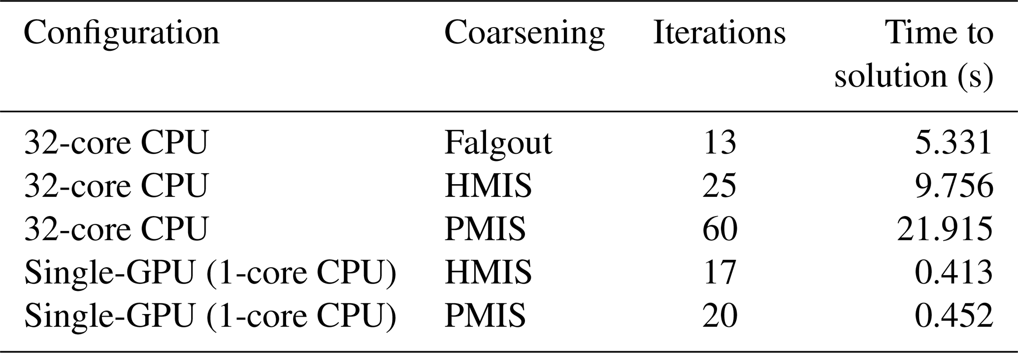
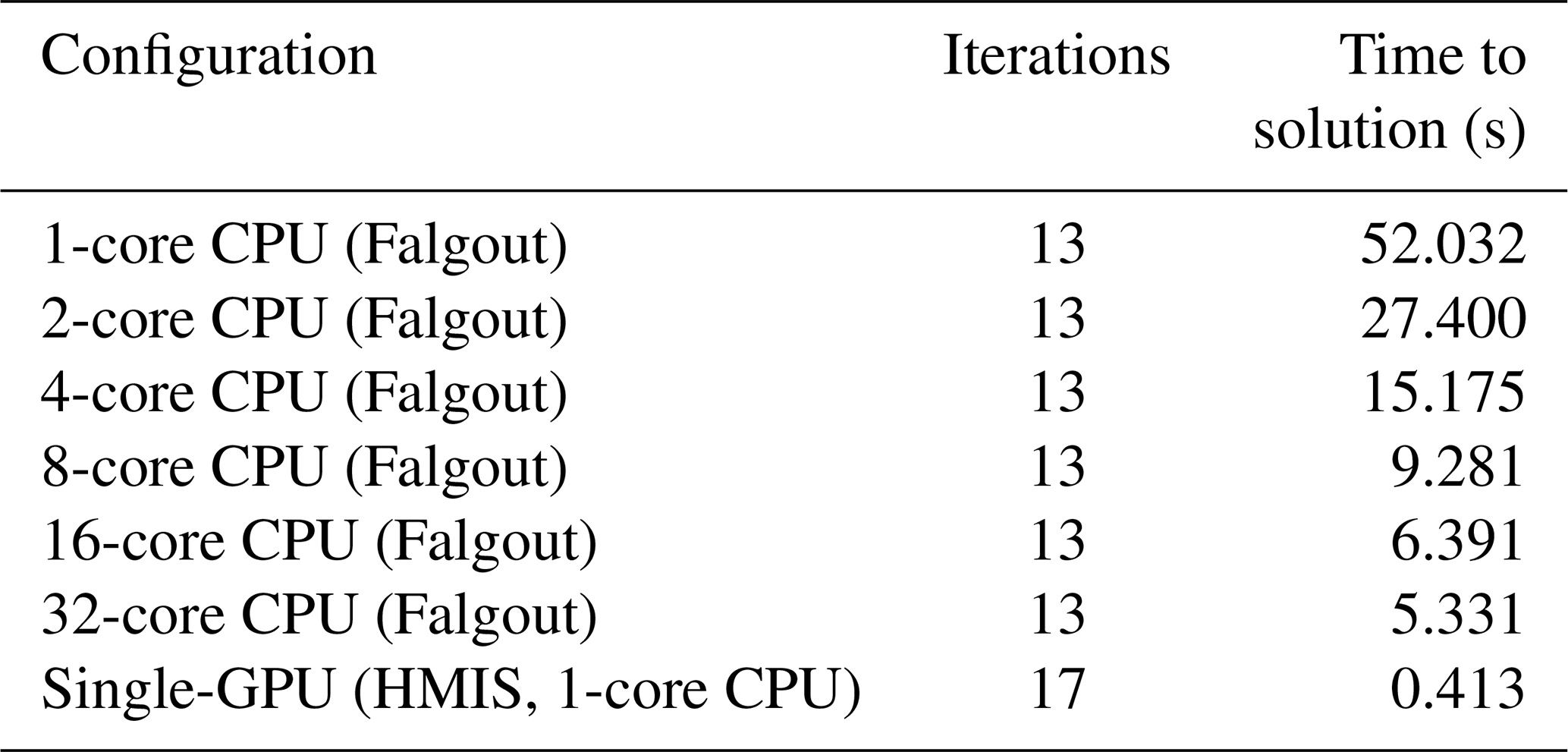
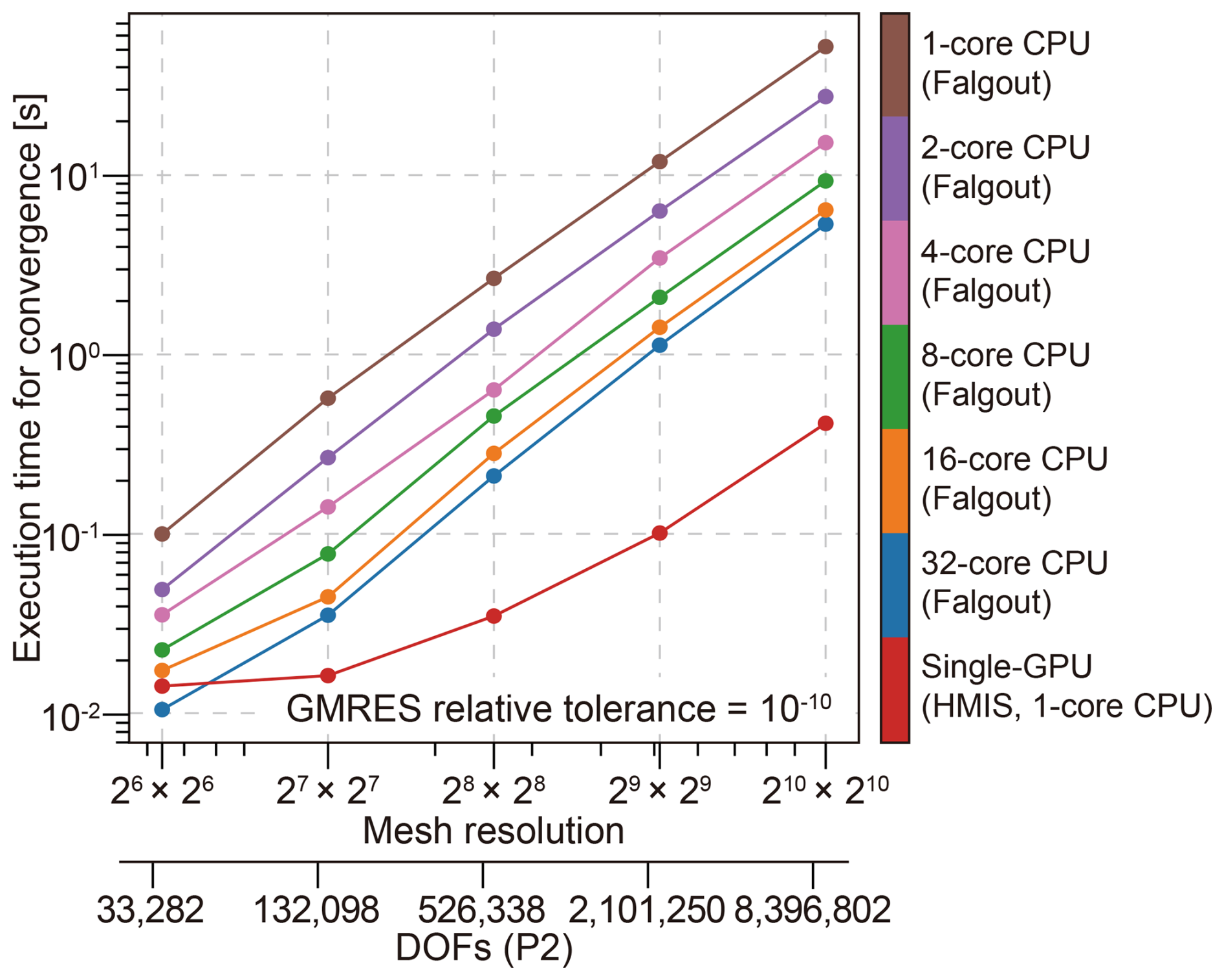
Figure 1 Inner GMRES solver execution time analysis for the velocity subproblem in single-GPU (HMIS) with 1-core CPU and multi-core CPU (Falgout) environments. Total execution time to convergence with respect to increasing mesh resolution for the GPU and CPU.

4.2 SolCx problem

We used the 2D SolCx benchmark, which has been widely employed to assess the stability and convergence of GPU Stokes solvers with strong viscosity discontinuities (Zhong, 1996; Duretz et al., 2011; Kronbichler et al., 2012; Gerya et al., 2013). The computational domain is the unit square $\mathrm{\Omega }=[\mathrm{0},\mathrm{1}]\times [\mathrm{0},\mathrm{1}]$ with free-slip boundary conditions on all four sides. The density field was prescribed to vary smoothly. In contrast, the viscosity exhibited a sharp jump at x=0.5 (Eq. 19). We set Ra to 0 and Rb to a spatially varying field to generate buoyancy (Eq. 20). A single composition field was adopted with C₀=1.

$$\begin{array}{}\text{(19)}& {\displaystyle }\mathit{\eta }\left(x\right)=\left\{\begin{array}{ll}\mathrm{1},& \mathrm{0}\le x\le \mathrm{0.5},\\ {\mathrm{10}}^{\mathrm{6}},& \mathrm{0.5}<x\le \mathrm{1}.\end{array}\right.\text{(20)}& {\displaystyle }{\displaystyle }\mathit{Rb}(x,y)=-\sin \left(\mathit{\pi }y\right){\displaystyle }\cos \left(\mathit{\pi }x\right),\mathrm{0}\le x\le \mathrm{1},\mathrm{0}\le y\le \mathrm{1}\end{array}$$

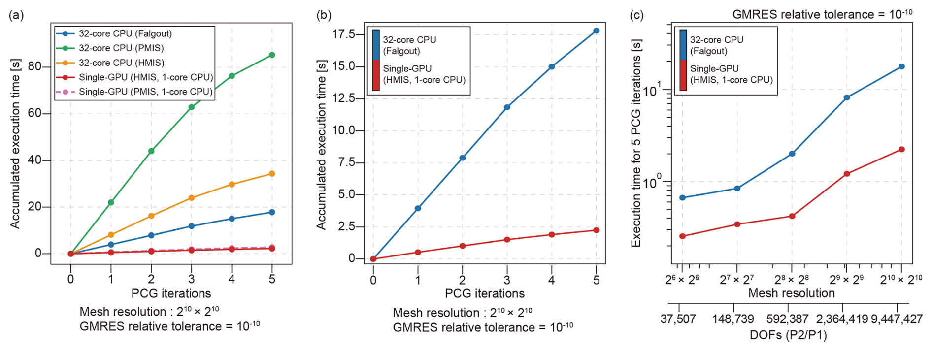
Figure 2 Execution time analysis of the SolCx benchmark in GPU and CPU environments. (a) Accumulated execution times on the GPU and 32-core CPU under different AMG preconditioner coarsening schemes (Falgout, PMIS, and HMIS). (b) Accumulated execution time on the single-GPU (HMIS) and 32-core CPU (Falgout). (c) Execution time for five preconditioned conjugate-gradient (PCG) iterations with increasing mesh resolution on the single-GPU (HMIS) and 32-core CPU (Falgout).

The viscosity jump of 10⁶ restricts the flow to the low-viscosity half, with the pressure discontinuous across the interface (Fig. S2). We compared the performance of the GPU-accelerated finite-element model with that of the 32-core CPU. The GMRES solver employed a default relative tolerance of 10⁻¹⁰. Performance was tested with varying GMRES relative tolerance and mesh resolution, based on the execution time of the PCG solver and velocity error relative to the analytical solution. The number of PCG iterations was fixed at five. After five PCG iterations, the L₂-error relative to the analytical solution was smaller than 10⁻⁹ for both GPU and 32-core CPU configurations.

We found that the performance of the velocity-only subproblem translated directly into the PCG solver performance (Fig. 2a). HMIS on the GPU and Falgout on the CPU were the most effective choices. In all cases, PCG solver execution time on the single-GPU was shorter than that on the 32-core CPU (Fig. 2a). The GPU achieved an approximately 8× speedup over the 32-core CPU, demonstrating the high efficiency of the GPU architecture. Based on the comparison in Fig. 2a, the HMIS and Falgout coarseners delivered the best performance on a single-GPU and a 32-core CPU, respectively. Thus, the HMIS and Falgout coarseners were used for single-GPU and 32-core CPU performance comparisons in Fig. 2b and c. Then, we compared accumulated execution times for five PCG iterations on a single-GPU and 32-core CPU (Fig. 2b). The single-GPU recorded the shortest execution time at 2.25 s.

The performance evaluation with increasing problem sizes exhibited a similar trend (Fig. 2c). As the resolution increased, the gap between the GPU and CPU execution times widened. For all resolutions, the single-GPU delivered shorter execution times than the 32-core CPU environment. This advantage of the GPU was more pronounced for larger problems (Fig. 2c). For the highest resolution (1024×1024, 9 447 427 DOFs), the GPU required 2.25 s, while the 32-core CPU required 17.82 s, corresponding to a speedup of approximately 7.9×. The single GPU reached a throughput of 4.2×10⁶ DOFs s⁻¹, compared with 5.3×10⁵ DOFs s⁻¹ on the 32-core CPU. In the memory bandwidth benchmark (Table S1), the GPU sustains 824.0 GB s⁻¹ and the 32-core CPU sustains 113.2 GB s⁻¹, a ratio of 7.3×. The sustained ratio exceeds the theoretical peak ratio of 6.25× (960 and 153.6 GB s⁻¹). The speedups measured across the Stokes benchmarks span 6–11× and cluster around the sustained ratio. The cost of PCG and GMRES is dominated by sparse matrix-vector products, data-parallel operations that map onto the GPU, where high memory bandwidth sustains the streaming access pattern. The unequal fractions of peak bandwidth attained by the GPU and CPU (86 % and 74 %, respectively) widen the sustained ratio beyond the peak ratio. The CPU and GPU versions of BoomerAMG further adopt different coarsening strategies that shift the number of iterations. The measured speedup depends on the cost per iteration and on the number of iterations. The sustained ratio serves as an approximate reference rather than an upper bound.

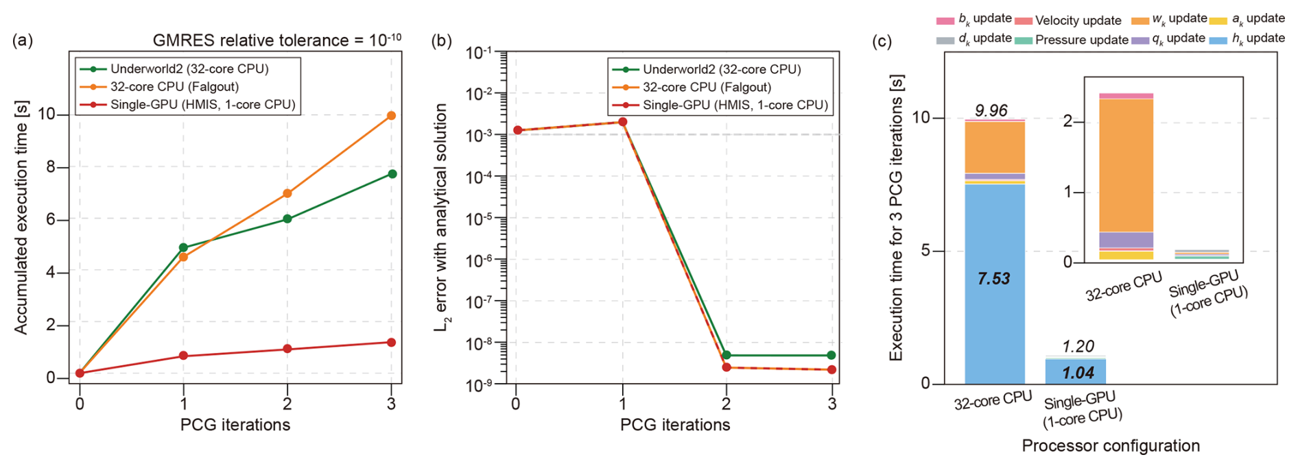
Figure 3 Performance benchmark and detailed execution time analysis of the preconditioned conjugate-gradient (PCG) iterations for the SolCx benchmark. (a) Comparison of accumulated execution time as a function of the number of PCG iterations for single-GPU (HMIS) with 1-core CPU, Underworld2 (Mansour et al., 2020; 32-core CPU), and 32-core CPU (Falgout) environments. (b) Comparison of the L₂-error with respect to the analytical solution as a function of the number of PCG iterations for single-GPU (HMIS) with 1-core CPU, Underworld2 (32-core CPU), and 32-core CPU (Falgout) environments. (c) Breakdown of execution time over 3 PCG iterations for the single-GPU with 1-core CPU and 32-core CPU.

Figure 3a presents the accumulated execution times for the PCG solver on a single-GPU (red line) and a 32-core CPU environment (orange line). Both environments fixed the number of PCG iterations at three. Underworld2 (Mansour et al., 2020) was evaluated on a 32-core CPU using the default settings, including $Q_{\mathrm{1}}/d{Q}_{\mathrm{0}}$ quadrilateral elements, at a 2048×2048 resolution. Three pressure-correction iterations were used to solve the Schur-complement system. The velocity-only subsystem was solved using GMG-preconditioned GMRES. In Underworld2, the cumulative execution time over the three iterations was 7.7 s. For comparison with Underworld2, our FEniCS calculations used triangular $P_{\mathrm{1}}/P_{\mathrm{0}}$ elements at the same 2048×2048 resolution. Over three PCG iterations, the single GPU required 1.2 s, whereas the 32-core CPU required 9.96 s. The single GPU was therefore 6.42× faster than Underworld2 and 8.3× faster than the 32-core CPU implementation.

We measured the L₂-error against the analytical solution with respect to PCG iteration number (Fig. 3b). All three configurations reduced the L₂-error below 10⁻⁸ after the second pressure-correction iteration. The final converged error from the PCG solver was lower than that of Underworld2. This difference is attributed to the larger number of DOFs associated with the P₀ element used in FEniCS (8 388 608 DOFs) compared to the dQ₀ element used in Underworld2 (4 194 304 DOFs).

We measured execution times for individual stages of the PCG solver algorithm (solving velocity-only subsystem, vector update, and projection) to quantify differences between the 32-core CPU run and the GPU run (Fig. 3c). The single-GPU achieved an overall speedup of 8.3× relative to the 32-core CPU. The velocity-only subsystem stage dominated the total cost, with 7.53 s of the 9.96 s on the CPU and 1.04 s of the 1.20 s on the GPU, a speedup of 7.2×. The speed of the vector update and projection stages is limited by memory bandwidth. The high memory bandwidth of the GPU reduced the time of the two stages from approximately 2.4 s on the CPU to 0.16 s.

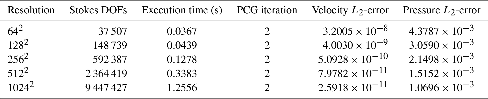
We measured the execution time to convergence while decreasing the GMRES relative tolerance from 10⁻⁴ to 10⁻¹⁰ (Fig. 4a). The single-GPU and 32-core CPU configurations attain the minimum execution times at 10⁻⁵, with execution time increasing at smaller tolerances. The single-GPU maintains the lowest execution time across the tested range, requiring 0.6–1.7 s compared with 5.4–15.2 s on the 32-core CPU. The number of outer PCG iterations decreases from seven at 10⁻⁴ to two at 10⁻⁵ and remains at two for smaller tolerances. The 7 PCG iterations at 10⁻⁴ cost more execution time than the 2 iterations at 10⁻⁵ on both configurations. A GMRES relative tolerance smaller than 10⁻⁴ delivers both the lower outer PCG iteration number and the shorter execution time. The single-GPU and 32-core CPU require an identical number of outer PCG iterations at each tolerance. For GMRES relative tolerances of 10⁻⁵ and smaller, the outer PCG iteration count remains fixed at two. Changes in total execution time therefore reflect the computational cost per outer iteration. We also calculated the L₂ errors relative to the analytical solution over the tested tolerance range (Fig. 4b). The velocity error generally decreases as the GMRES relative tolerance is tightened, reaching the order of 10⁻¹¹ at 10⁻⁸ and remaining at a similar level for tighter tolerances. Below 10⁻⁸, the execution time continues to increase without further improvement in velocity accuracy. The pressure error plateaus near 10⁻³ for GMRES relative tolerances below 10⁻⁸. A GMRES relative tolerance of 10⁻⁸ therefore provides converged accuracy without the additional computational cost associated with smaller tolerances. The outer PCG solver converged in two iterations across resolutions from 64² to 1024² on the single-GPU (Table 4) and 32-core CPU (Table 3), indicating mesh-independent convergence of the Schur-complement iteration. The lower convergence rate of the pressure L₂ error with mesh refinement reflects the pressure discontinuity in the SolCx benchmark and the use of a continuous P₁ pressure approximation.

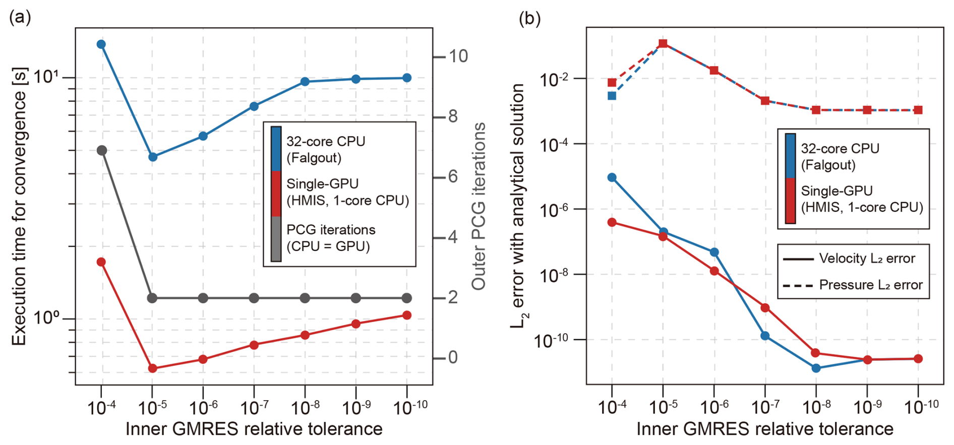
Figure 4 PCG solver performance across inner GMRES relative tolerances for the SolCx benchmark at a 2¹⁰×2¹⁰ resolution. (a) Execution time to convergence on the single-GPU (HMIS, red line) and 32-core CPU (Falgout, blue line), with the number of outer PCG iterations (grey line). The number of outer PCG iterations for convergence is identical for both configurations. (b) L₂ errors of the velocity (solid) and pressure (dashed) solutions relative to the analytical solution for the single-GPU and 32-core CPU configurations.

Table 3 Execution time, outer PCG iteration number, and L₂ errors with increasing mesh resolution for the SolCx benchmark on a 32-core CPU. The GMRES relative tolerance and divergence tolerance are 10⁻¹⁰ and 10⁻⁶, respectively.

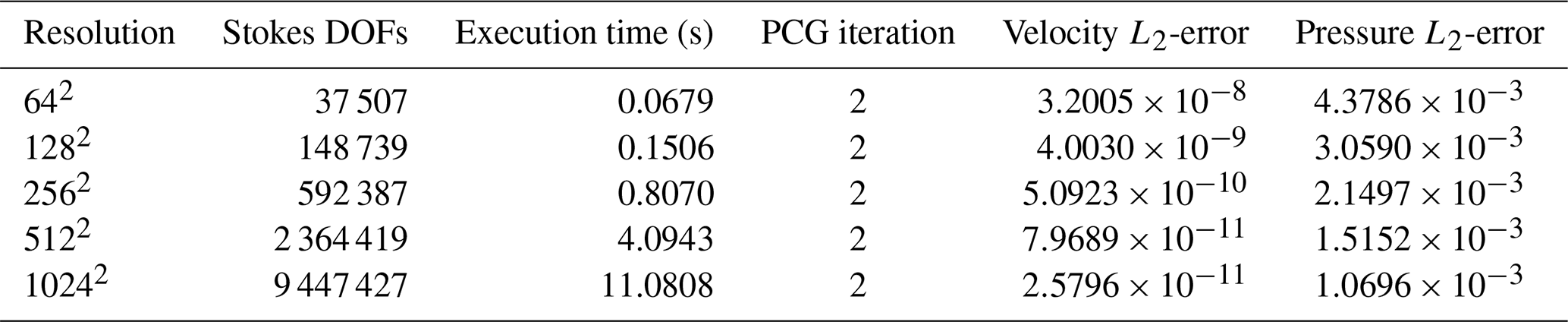
Table 4 Execution time, outer PCG iteration number, and L₂ errors with increasing mesh resolution for the SolCx benchmark on a single-GPU. The GMRES relative tolerance and divergence tolerance are 10⁻¹⁰ and 10⁻⁶, respectively.

4.3 3D Thermo-mechanical convection

We extended the classical 2D thermo-mechanical convection benchmark of Blankenbach et al. (1989) to a 3D non-rotating Boussinesq fluid to evaluate the performance and memory usage of the GPU solver in three dimensions. The thermal and compositional Rayleigh numbers were set to Ra=10⁴ and Rb=0 in Eq. (1), isolating thermal effects by neglecting compositional buoyancy. A 3D rectangular domain ($\mathrm{1}\times \mathrm{0.4}\times \mathrm{1}$) was employed to quantitatively compare computational performance and velocity-field accuracy between the GPU and CPU environments. The grid resolution was set to $\mathrm{100}\times \mathrm{40}\times \mathrm{100}$ using the MINI element ($P_{\mathrm{1}}^{+}\times P_{\mathrm{1}}$), yielding approximately 8.9 million DOFs for velocity and pressure. Free-slip boundary conditions were applied to all boundaries. For the temperature boundary conditions, nondimensional temperatures of T=0 and T=1 were prescribed at the top and bottom boundaries, respectively. The initial temperature field T₀ consisted of a linear conductive profile with a superimposed long-wavelength perturbation of amplitude α=0.02 to initiate natural convection (Eq. 21). As time proceeds, thermal plumes rise from the lower boundary, which leads to a progressive reorganization of the internal temperature field and the heat-flow pattern at the boundaries (Fig. 5).

$$\begin{array}{}\text{(21)}& T_{\mathrm{0}}=\mathrm{1}-z+\mathit{\alpha }\cos \left(\mathit{\pi }x\right)\sin \left(\mathit{\pi }z\right)\end{array}$$

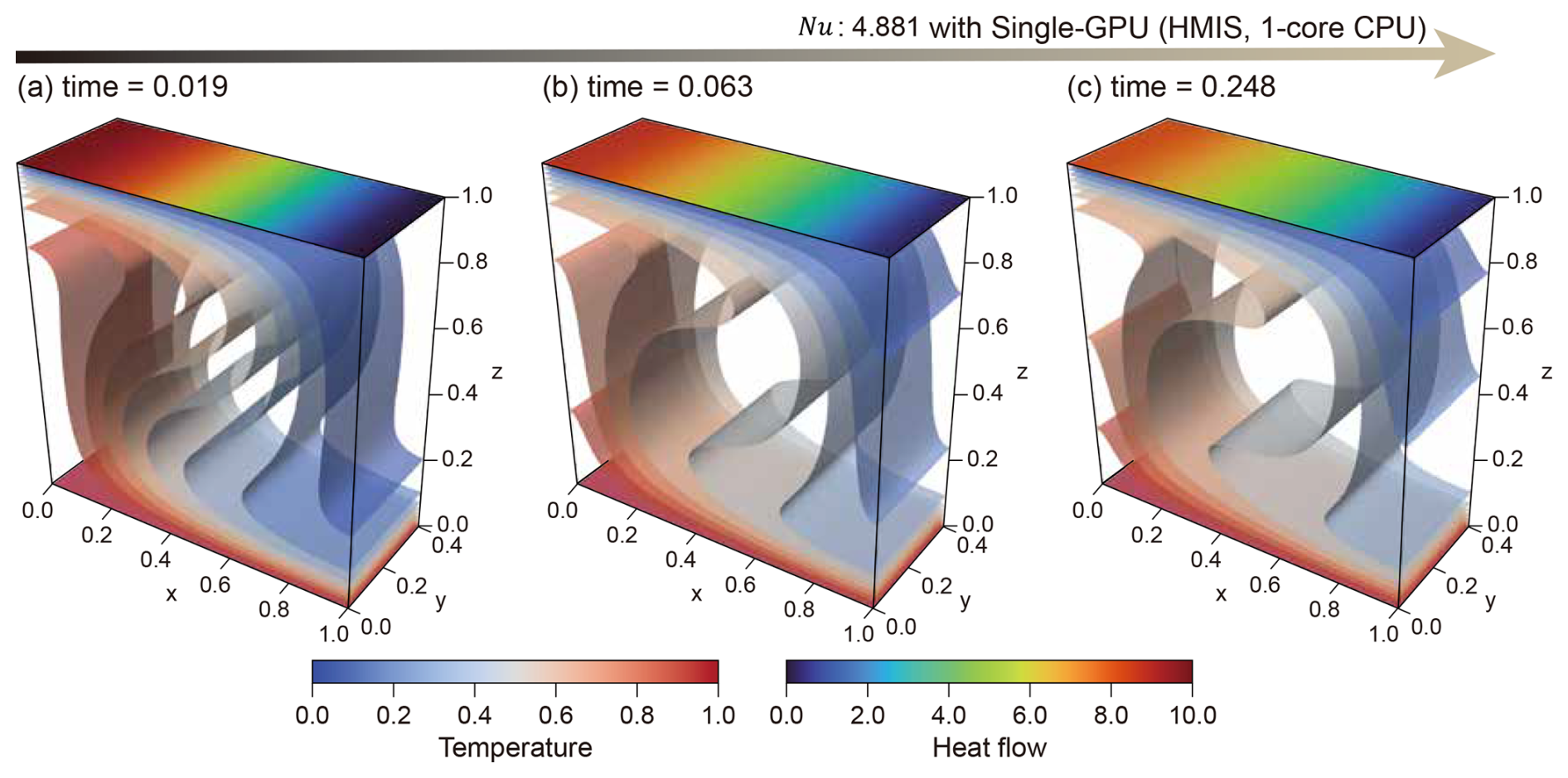
Figure 5 Time evolution of the temperature field from the single-GPU (HMIS) with 1-core CPU. Snapshots of 3D temperature isosurfaces at nondimensional times t=0.019, 0.063, and 0.248 (from left to right).

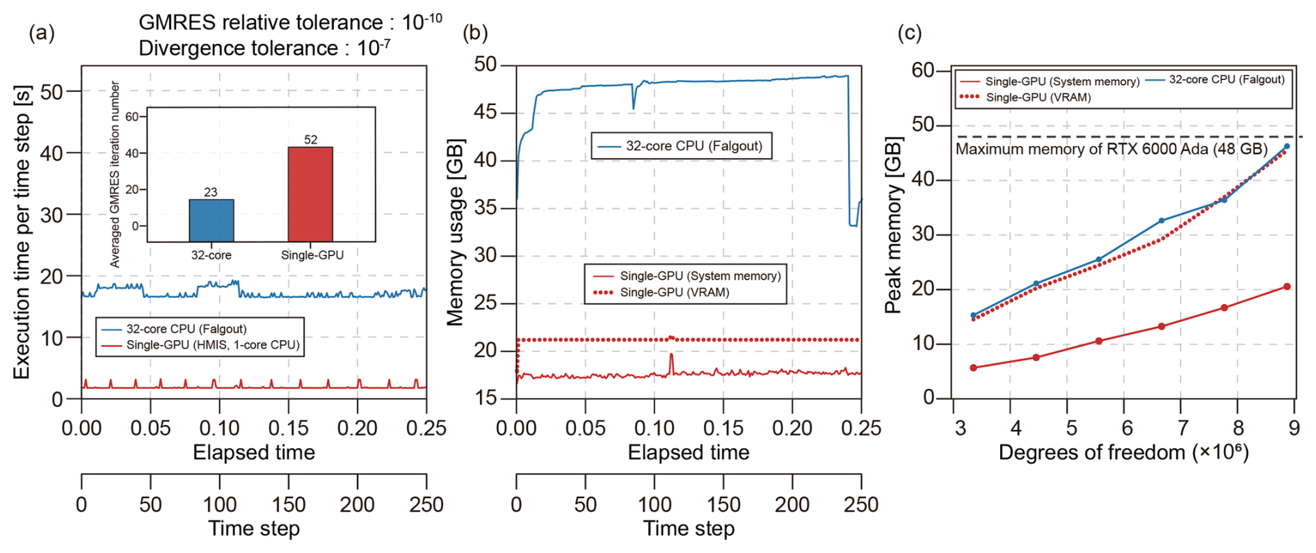
Figure 6 Performance analysis and validation of the 3D thermo-mechanical convection simulation. (a) Execution time per step (solid lines) and averaged GMRES iteration numbers (inset bar chart) versus elapsed time. (b) Evolution of memory usage over elapsed time, showing GPU VRAM (dotted red line), system memory of the GPU workstation (solid red line), and system memory of the CPU workstation (solid blue line). (c) Peak memory usage with respect to increasing degrees of freedom (DOFs), with the dashed black line indicating the 48 GB VRAM capacity of the NVIDIA RTX 6000 Ada.

We utilised a fixed time step (Δt=0.00025) with the Crank–Nicolson scheme for time integration. We set the GMRES relative tolerance to 10⁻¹⁰ for the velocity-only subsystem on both GPU and CPU, continuing the PCG iterations until the divergence error ($\parallel \mathrm{\nabla }\cdot \mathit{u}\parallel /\parallel \mathit{u}\parallel$) fell below 10⁻⁷. The energy equation (Eq. 4) was solved using GMRES with a relative tolerance of 10⁻⁸, utilising BoomerAMG as the preconditioner, configured with HMIS for the GPU and Falgout for the CPU, respectively.

For the Stokes equations, the single-GPU (HMIS) achieved the lowest execution time with an average of 1.9 s (Fig. 6a; solid red line), compared with 17.1 s for the 32-core CPU (Falgout) (solid blue line). The speedup relative to the 32-core CPU was approximately 9×. At 8.87×10⁶ DOFs, the average execution time per step corresponds to a throughput of 4.7×10⁶ DOFs s⁻¹ on the single GPU and 5.2×10⁵ DOFs s⁻¹ on the 32-core CPU. The average number of GMRES iterations per time step was 52 on the GPU and 23 on the 32-core CPU (Fig. 6a, coloured bars). The GPU exhibited shorter execution time per time step despite the iteration number being 2.3× higher than the CPU baseline. Memory usage measurements for the GPU environment included both VRAM and system memory (RAM) of the workstation (Fig. 6b). The average VRAM and system memory usage per time step were 21.2 GB (dotted red line) and 17.4 GB (solid red line), respectively, for a total of 38.6 GB. In the CPU environment, the average memory usage was 46.3 GB on the 32-core CPU, approximately 1.20× the total memory usage of the single-GPU configuration.

The temporal evolution of the global root-mean-square velocity (V_rms) exhibited complete consistency between the GPU and 32-core CPU environments (see Fig. S3). The measurements converged to 42.848, consistent with the value of 42.865 reported by Blankenbach et al. (1989). A Nusselt number (Nu) of 4.881 was calculated at the final time step in both configurations, matching the value of 4.884 presented in benchmark studies (Blankenbach et al., 1989; Tackley and King, 2003; King, 2009). To assess memory constraints associated with the multi-level generation of the AMG preconditioner, we measured the maximum memory usage for each computing environment with increasing mesh resolution (Fig. 6c). Measurements for the GPU environment included both VRAM and system memory. At the lowest DOFs (3 352 864), VRAM and system memory usage were 14.5 and 5.7 GB, respectively. At the highest DOFs (8 872 964), VRAM usage reached 45.5 GB, while system memory usage reached 20.6 GB. The 32-core CPU registered 15.3 GB at the lowest DOFs and 47.3 GB at the highest, exhibiting levels comparable to the GPU VRAM usage.

4.4 2D Rayleigh–Taylor instability

The Rayleigh–Taylor instability is a buoyancy-driven flow widely used as a benchmark for evaluating the performance of various advection schemes. Representative approaches include Particle-In-Cell (PIC) methods (e.g., Gerya and Yuen, 2003; van Keken et al., 1997) and level-set methods (e.g., Bourgouin et al., 2006). We set Ra=0 and Rb=1, indicating that only compositional buoyancy is activated. The initial interface between the two compositions is defined by a cosine function with an amplitude of 0.02 (Eq. 22). The level-set function was initialized (Eq. 23) from the interface at t=0. The composition field was set to 1 and 0 where the level-set function was positive and negative (Eq. 24), respectively. The level-set function was reinitialised every 500 steps.

$$\begin{array}{}\text{(22)}& {\displaystyle }h\left(x\right)=\mathrm{0.02}\cos (\mathit{\pi }x/\mathrm{0.9142})+\mathrm{0.2}\text{(23)}& {\displaystyle }\mathit{\varphi }(x,y,t=\mathrm{0})=y-h\left(x\right)\text{(24)}& {\displaystyle }C(x,y,t=\mathrm{0})=\left\{\begin{array}{ll}\mathrm{0},& \mathit{\varphi }(x,y,t=\mathrm{0})\le \mathrm{0},\\ \mathrm{1},& \mathit{\varphi }(x,y,t=\mathrm{0})>\mathrm{0}\end{array}\right.\end{array}$$

For resolving complex velocity and composition structures, we adopted uniform grids with 512×512 resolution. The Taylor-Hood element (P₂×P₁) was applied to solve the Stokes equations. We compared the V_rms values computed by our FEniCS code with those from previous benchmark models (van Keken et al., 1997; Hillebrand et al., 2014). The advection equation for the level-set function was solved using GMRES preconditioned by HYPRE's BoomerAMG. The average per-step execution time was compared across GPU and CPU environments in the 2D benchmark (Fig. 7a). The GPU completed one step in 0.6 s on average (0.53 s for the Stokes equations and 0.07 s for advection), yielding speedups of $\sim \mathrm{11}\times$ relative to the 32-core CPU, which required 6.3 s per step. The per-step cost was dominated by solving the Stokes equations (6.2 s for the 32-core CPU). The Stokes solve at 512×512 (2.36×10⁶ DOFs) reached a throughput of 4.5×10⁶ DOFs s⁻¹ on the single GPU and 3.8×10⁵ DOFs s⁻¹ on the 32-core CPU. Despite the substantial improvement in computational efficiency enabled by GPU acceleration, the solution accuracy remains comparable to that of the CPU implementation. This agreement is demonstrated by the time evolution of V_rms, which closely matches the CPU simulation (Fig. 7b). Snapshot comparisons at key times (t=208, 699, 864, and 1500), when V_rms attains local maxima or minima, further support the model accuracy. In addition, the GPU-based model reproduces the reference V_rms values from Hillebrand et al. (2014) and van Keken et al. (1997). We also tested the Rayleigh–Taylor instability in 3D on a $\mathrm{65}\times \mathrm{65}\times \mathrm{65}$ mesh with the MINI element. The single GPU delivered a speedup of $\sim \mathrm{9}\times$ relative to the 32-core CPU across the entire time range, while the two configurations produced identical V_rms values (Fig. S4).

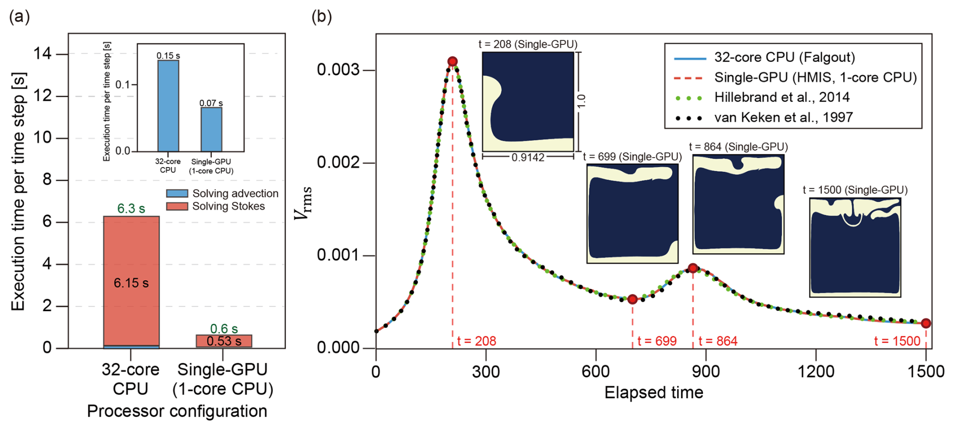
Figure 7 Performance analysis and accuracy validation of single-GPU (HMIS) with 1-core CPU and 32-core CPU (Falgout) configurations for the 2D Rayleigh–Taylor instability benchmark. (a) Execution time per step for solving the Stokes equations (red bars) and the advection equation (blue bars) across GPU and 32-core CPU configurations. (b) Time evolution of the root-mean-square velocity (V_rms) compared with literature benchmarks (van Keken et al., 1997; Hillebrand et al., 2014). The inset snapshots represent the composition fields computed on the GPU at key time steps (t=208, 699, 864, and 1500).

4.5 Sticky-air benchmarks

In geodynamic numerical modelling, the sticky-air technique is a widely used approach for approximating a free surface. Crameri et al. (2012) suggested that to correctly represent a free-surface boundary condition, the sticky-air layer requires a viscosity contrast of 10⁻⁵ relative to the underlying material and a thickness of 100 km, or alternatively a viscosity contrast of 10⁻⁴ and a thickness of 200 km. In our study, we set the viscosities of the lithospheric, mantle, and sticky-air layers (with a thickness of 100 km) to η_litho=10²³ Pa s, η_mantle=10²² Pa s, and η_air=10¹⁸ Pa s, respectively. Buoyancy in the sticky-air benchmark is purely compositional. The isothermal configuration of Crameri et al. (2012) fixes Ra=0 in the absence of a temperature field, leaving Eq. (4) outside the solution. The benchmark constrains the free-surface response alone, with the thermo-mechanical benchmark held separate. The dimensional parameters for the sticky-air benchmark are presented in Table S3. We discretized the Stokes system using P₂×P₁ finite elements on a 1400×800 mesh. The boundary between the lithosphere and the sticky-air was assigned a cosine-shaped perturbation. We compared the maximum topography with the analytical solution from Crameri et al. (2012). The initial composition field (C) is defined as three layers separated by the upper and lower interfaces of the lithosphere (Eq. 25). C₁, C₂, and C₃ denote sticky-air, lithosphere, and mantle, respectively. Two level-set functions (ϕ₁ and ϕ₂) were defined for the two interfaces (Eqs. 26 and 27).

$$\begin{array}{}\text{(25)}& {\displaystyle }C=\left\{\begin{array}{ll}{C}_{\mathrm{1}},& {\mathit{\varphi }}_{\mathrm{1}}(x,y,t=\mathrm{0})\le \mathrm{0}\\ C_{\mathrm{3}},& {\mathit{\varphi }}_{\mathrm{2}}(x,y,t=\mathrm{0})<\mathrm{0}\\ C_{\mathrm{2}},& \text{else}\end{array}\right.\text{(26)}& {\displaystyle }{\mathit{\varphi }}_{\mathrm{1}}(x,y,t=\mathrm{0})=\mathrm{700}+\mathrm{7}\cos \left({\displaystyle \frac{\mathrm{2}\mathit{\pi }x}{\mathrm{2800}}}\right)-y\text{(27)}& {\displaystyle }{\mathit{\varphi }}_{\mathrm{2}}(x,y,t=\mathrm{0})=y-\mathrm{600}\end{array}$$

An initial perturbation imposed on the lithosphere generates a lateral density gradient, which drives upwelling in the centre of the domain and downwelling on both sides, forming two convection cells (Fig. 8a). Advective transport progressively flattens the initial topographic perturbation. At 5.77 kyr, the decaying perturbation weakens the flow in the two convection cells (Fig. 8b). The surface recovers an almost flat geometry by the final time of 100 kyr (Fig. 8c). In contrast, the divergence-free dynamics of mantle and lithosphere flow advect the initially horizontal lithosphere–mantle boundary, producing a secondary perturbation by the final time (Fig. 8c). The maximum topography over the simulation time was identical between the GPU and CPU executions (Fig. 8). The topographies from the CPU and GPU are consistent with the analytical solution and the reported curve of Hillebrand et al. (2014), indicating that the physical solution on GPU remains consistent despite the larger number of GMRES iterations.

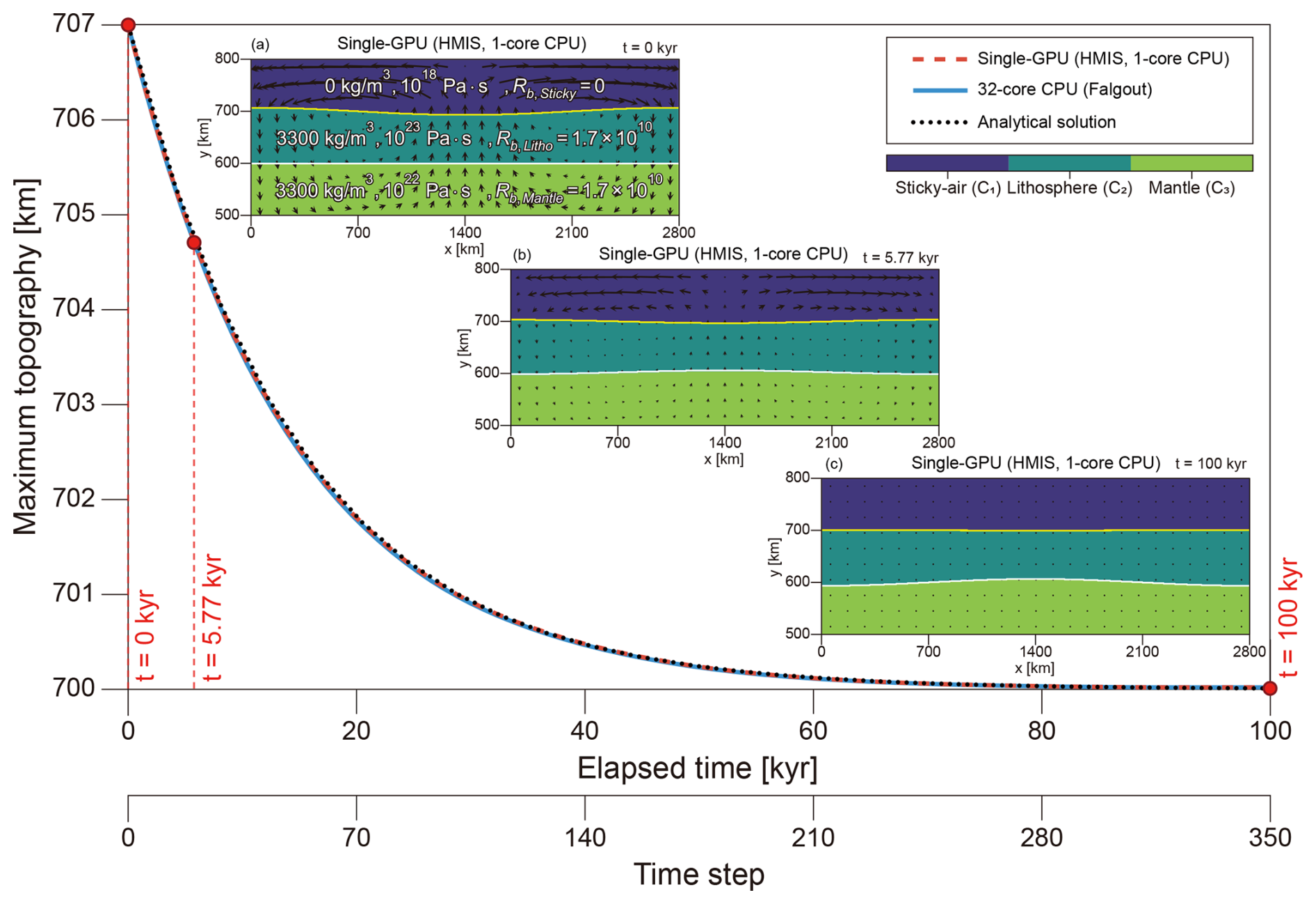
Figure 8 Evolution of maximum topography in the sticky-air benchmark. The dashed red line denotes the single-GPU (HMIS) with 1-core CPU, the solid blue line denotes the 32-core CPU computation, and the dotted black line denotes the analytical solution. (a–c) Temporal evolution of the compositional field at t=0, 5.77, and 100 kyr, respectively, from the single-GPU (HMIS, 1-core CPU). The temporal evolution of maximum topography indicates close agreement between the GPU and CPU computations and with the analytical solution.

Execution time comparison over the total steps shows that the GPU consistently outperformed the 32-core CPU (Fig. 9a). The GPU (HMIS) execution time remained stable within 4.7–11.1 s, whereas the CPU (Falgout) execution time increased from 30 s to more than 100 s (Fig. 9a; solid blue line), corresponding to an overall speedup of roughly 7–8× for the GPU (solid red line). At 1.01×10⁷ DOFs, the per-step execution time corresponds to a throughput of 0.9–2.1×10⁶ DOFs s⁻¹ on the single GPU and 1.0–3.4×10⁵ DOFs s⁻¹ on the 32-core CPU. The number of PCG iterations varied with simulation time, while the GPU and CPU generally required similar numbers of PCG iterations at each time step (Fig. 9b). Time steps with a larger number of PCG iterations also exhibited a larger number of GMRES iterations within the iteration loop. The GPU and CPU required 250–650 and 150–410 GMRES iterations, respectively.

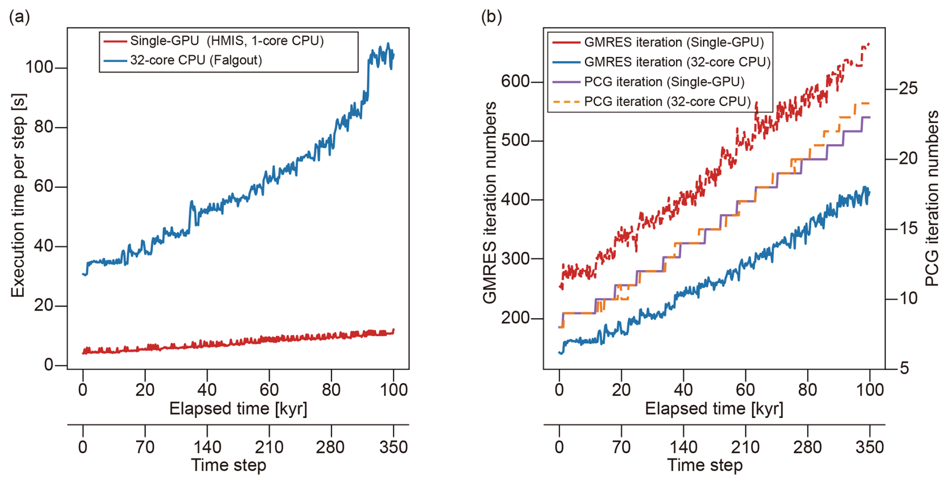
Figure 9 Performance analysis and accuracy validation of the sticky-air benchmark. (a) Execution time per step over elapsed time for the single-GPU (HMIS) with 1-core CPU and 32-core CPU (Falgout). (b) Evolution of inner GMRES iteration numbers (left axis) and preconditioned conjugate-gradient (PCG) iteration numbers (right axis).

4.6 Subduction modelling

The subduction application targets 2D nonlinear viscous Stokes flow incorporating a plate interface where one plate descends into the mantle. The computational domain is a rectangle with a width of 3960 km and a depth of 660 km, which is then nondimensionalized (Enns et al., 2005; Capitanio et al., 2010; Sharples et al., 2014). Characteristic scales for nondimensionalization are listed in Table S4. The Stokes system was discretized with P₂×P₁ elements on a 1200×200 structured grid, where each rectangular cell was subdivided into two triangular elements along the lower left to upper right diagonal. The compositional structure is partitioned into five regions: mantle, overriding plate, upper slab layer, lower slab layer, and slab core. Four level-set functions, ϕ₁ through ϕ₄, delineate the region interfaces.

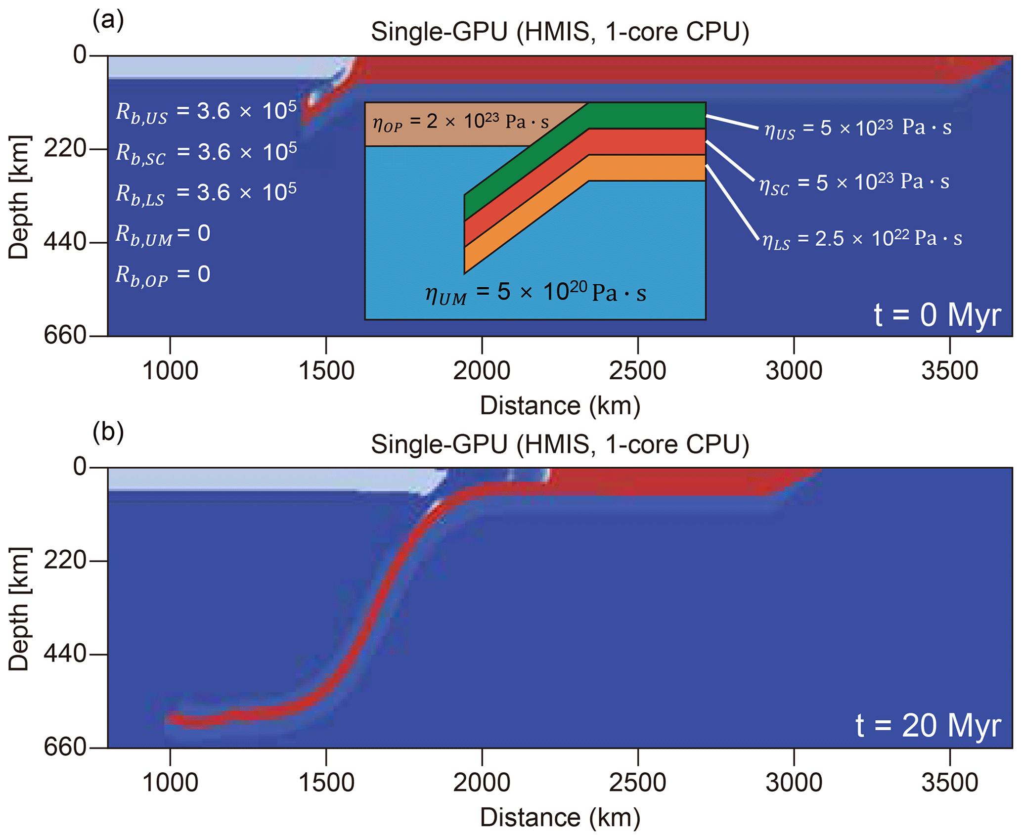
Figure 10 Temporal evolution of subduction modelling derived from the single-GPU (HMIS). (a) Initial model configuration at 0 Myr with the prescribed viscosity structure and buoyancy parameters. (b) Subduction geometry at 20 Myr after the slab descends into the upper mantle.

The upper mantle serves as the reference fluid with viscosity η_UM=1 and ρ=0. The overriding plate has the viscosity η_OP=400, yielding a viscosity contrast of 400 relative to the upper mantle, while its density matches the mantle value. The viscosity of the upper slab layer (η_US) follows a Mohr–Coulomb plasticity law (Eq. 28).

$$\begin{array}{}\text{(28)}& {\mathit{\eta }}_{\text{US}}={\displaystyle \frac{\mathrm{1}}{\mathrm{2}}}{\displaystyle \frac{{\mathit{\tau }}_y}{{\dot{\mathit{\epsilon }}}_{\text{II}}}},{\dot{\mathit{\epsilon }}}_{\text{II}}=\sqrt{{\displaystyle \frac{\mathrm{1}}{\mathrm{2}}}\dot{\mathit{\epsilon }}:\dot{\mathit{\epsilon }}}\end{array}$$

τ_y, $\dot{\mathit{\epsilon }}$, and ${\dot{\mathit{\epsilon }}}_{\text{II}}$ denote the plastic yield stress, strain-rate tensor, and the square root of its second invariant, respectively. τ_y was set to 0.06. η_US is bounded between 1 and 1000 to improve numerical stability. Additionally, at nondimensional depth y<0.7, weakening is imposed by prescribing η=50. The viscosities of the slab core (η_SC) and lower slab (η_LS) are 1000 and 50, respectively. Mohr–Coulomb plasticity in the upper slab layer introduces nonlinear viscosity into the Stokes system, requiring Picard fixed-point iteration with a relative tolerance of 10⁻³. As the viscosity contrast increases and compositional interfaces become more complex, the condition number of the discretized Stokes system tends to increase, degrading Krylov solver convergence. We therefore approximated the condition number at each time step using the ratio of the largest to smallest eigenvalues of the stiffness matrix and examined its relationship with the GMRES iteration number and execution time. An initial slab perturbation, pre-subducted to 200 km depth with a 29° dip, triggers subduction (Fig. 10a). The slab maintains a steep dip and ultimately reaches the base of the upper mantle (Fig. 10b).

The performance gap between the GPU and CPU persists in the subduction model. Over the full time-stepping sequence, the GPU reduces execution time by a factor of 6–7 relative to the 32-core CPU run (Fig. 11a). In geodynamic simulations, time evolution increases the spatial complexity of density and viscosity fields, often accompanied by large material contrasts. Such conditions worsen the system conditioning, increasing the condition number (purple line in Fig. 11a). Higher condition numbers require more GMRES iterations. In the subduction model, the estimated condition number increases with time step (Fig. 11a). As the condition number increases, execution time increases in both the GPU and CPU runs (Fig. 11b). However, the regression between GMRES iterations per step and condition number shows a steeper slope for the GPU (Fig. 11c). Despite this steeper slope, the GPU remains approximately 6× faster in execution time, as its lower per-iteration cost keeps the total execution time shorter. At 2.17×10⁶ DOFs, the throughput ranged from 1.1×10⁵ to 1.8×10⁵ DOFs s⁻¹ on the single GPU and from 1.4×10⁴ to 3.1×10⁴ DOFs s⁻¹ on the 32-core CPU. The Picard iterations within each step lower the throughput by an order of magnitude relative to the linear benchmarks.

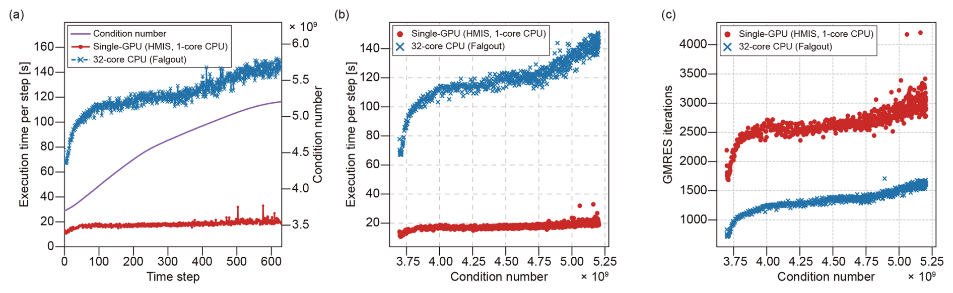
Figure 11 Analysis of GPU performance and matrix condition number for subduction modelling. (a) Evolution of the condition number and corresponding changes in execution time for single-GPU (HMIS) with 1-core CPU and 32-core CPU (Falgout) over time steps. (b) Correlation between the matrix condition number and execution time per step for the subduction model. (c) Correlation between the matrix condition number and inner GMRES iterations per step for the subduction model.

4.7 Multi-GPU implementation

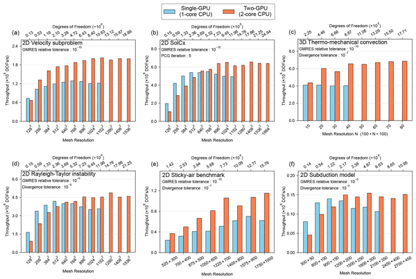
A multi-GPU configuration is essential to overcome the VRAM limit of a single-GPU. At high resolution, the growth in DOFs substantially increases the memory requirements for the stiffness matrix, the preconditioner, and the global force vector. Multi-GPU execution distributes VRAM usage via MPI-based domain decomposition, which also enables additional speedup through parallel execution. Inter-GPU communication and synchronization, however, introduce extra computational costs. We evaluated how throughput varies with resolution by comparing single-GPU and two-GPU configurations across six benchmarks in Sects. 4.1–4.6. In the velocity subproblem using P₂ elements, the single-GPU delivered higher throughput than the two-GPU configuration at the lowest resolution of 128×128 (1.32×10⁵ DOFs) (Fig. 12a). In the low-resolution regime, communication and synchronization overhead exceeded the performance gain from parallelization. At resolutions of 256×256 and higher, however, the two-GPU configuration delivered higher throughput than the single-GPU. In the high-resolution regime, the increased computational workload sufficiently outweighed the overhead, yielding a clear performance advantage for two-GPU runs. In addition, memory capacity limited the single-GPU to a maximum resolution of 1152×1152 (1.06×10⁷ DOFs), whereas the two-GPU configuration ran up to 1536×1536 (1.89×10⁷ DOFs). We compared the throughput of single-GPU runs with two-GPU runs across mesh resolutions for the SolCx benchmark using P₂×P₁ elements (Fig. 12b). In the high-resolution regime ($>\mathrm{512}\times \mathrm{512}$, corresponding to 2.36×10⁶ DOFs), the two-GPU configuration outperformed the single-GPU by a factor of 1.03 (for 640×640) to 1.31 (for 1024×1024). The two-GPU configuration supported a maximum resolution of 1664×1664 (24 936 707 DOFs), whereas the single GPU was limited by memory capacity to 1152×1152 (11 955 459 DOFs).

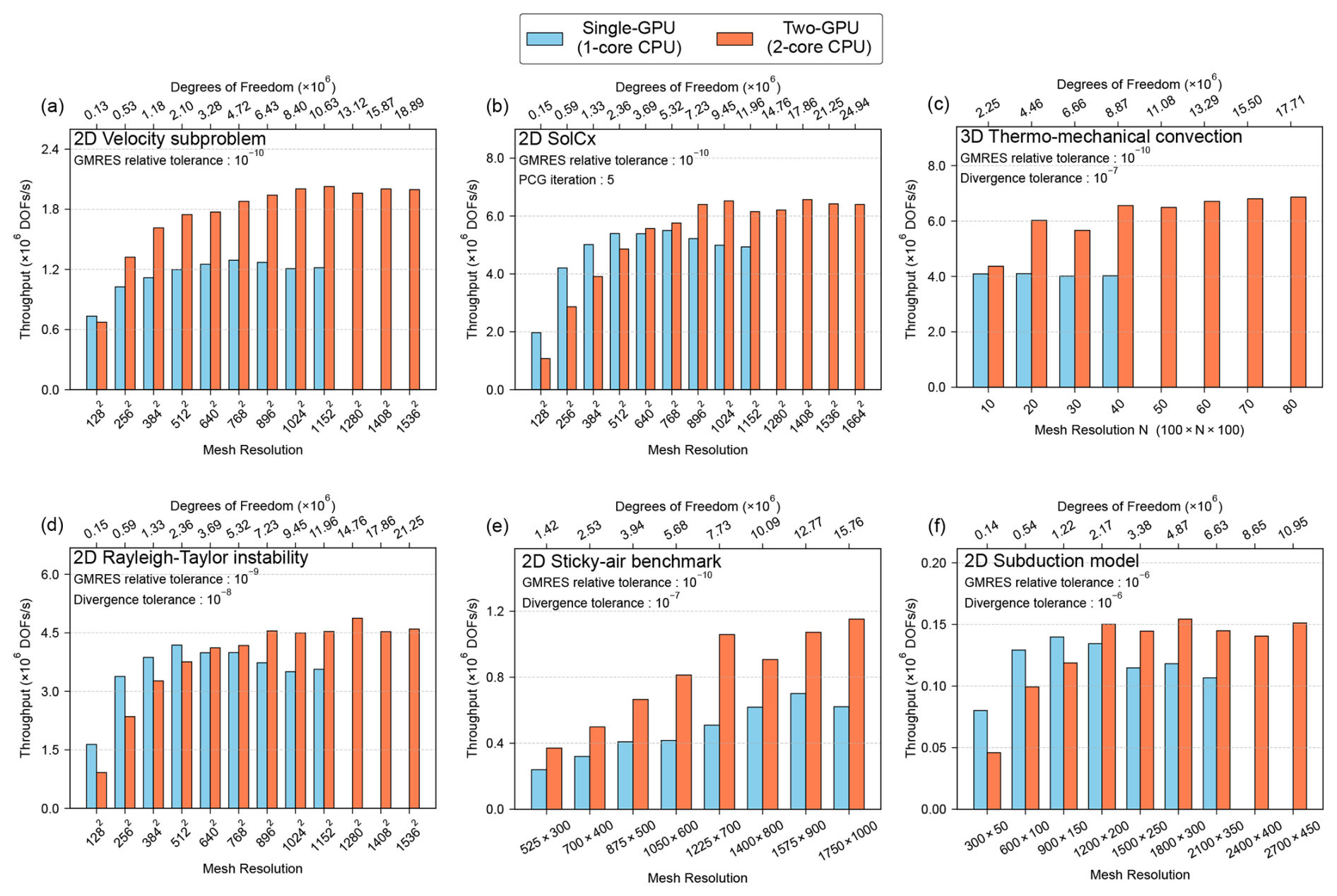
Figure 12 Performance comparison between single-GPU (1-core CPU) and two-GPU (2-core CPU) configurations in this study. (a–f) Comparison of throughput for the velocity subproblem, SolCx, 3D thermo-mechanical convection, 2D Rayleigh–Taylor instability, sticky-air benchmark, and subduction model, respectively. Horizontal axes represent mesh resolution and degrees of freedom; vertical axes represent throughput (DOFs s⁻¹).

For the 3D thermo-mechanical convection using the MINI element, the grid resolutions in the x and z directions were held fixed at 100 cells (Fig. 12c), while the y direction resolution increased from 10 to 80. The two-GPU configuration delivered higher throughput at every resolution. The throughput ratio increased from 1.07 to 1.64 as the resolution increased. The 2D Rayleigh–Taylor instability test with P₂×P₁ elements followed the same pattern as the 2D SolCx benchmark (Fig. 12d). The single-GPU delivered higher throughput at low resolution, whereas the two-GPU throughput exceeded the single-GPU throughput beyond 512×512. In the sticky-air benchmark, the two-GPU configuration delivered higher throughput than the single-GPU at all resolutions (Fig. 12e). The throughput ratio ranged from 1.5 to 2.1. In the subduction model with nonlinear viscosity, the two-GPU throughput exceeded the single-GPU throughput beyond 900×150. Then, the two-GPU throughput reached 1.4 times the single-GPU throughput (Fig. 12f). The single-GPU delivered higher throughput at low resolution in the SolCx, 2D Rayleigh–Taylor, and subduction benchmarks. Once the DOFs exceeded a threshold, the computational workload dominated, reducing the relative impact of overhead, and the two-GPU configuration became more effective. In 3D problems, the number of DOFs increases more rapidly with mesh resolution, yielding a consistent advantage for the two-GPU configuration across the tested resolutions.

5 Discussion

5.1 Efficiency of pre-assembled operators

In this study, we present a practical strategy to reduce bottlenecks in a single-GPU workflow, where one CPU core assembles matrices and the GPU performs iterative solves. Before performing GPU-based PCG solves, the L₂-projection mass matrix, gradient operator, and divergence operator are assembled once on the CPU and stored in GPU VRAM. Pre-assembly of the three operators removes the assembly cost from every PCG iteration. The end-to-end throughput of each time step therefore increases. The approach becomes increasingly beneficial when many PCG steps are nested inside Picard iterations. The benefits are most pronounced for iteration-heavy workloads, such as the Picard iterations for the nonlinear-viscosity subduction model (Sect. 4.6). We note that the stiffness matrix must still be reassembled when viscosity changes between time steps. Storing preassembled operators increases VRAM requirements as the number of DOFs increases. For an incompressible Stokes system on a fixed mesh, the gradient and divergence operators for velocity–pressure coupling remain constant across iterations. For example, at a $\mathrm{100}\times \mathrm{40}\times \mathrm{100}$ resolution with the MINI element for the 3D thermo-mechanical convection benchmark (Sect. 4.3), storing these operators and associated vectors requires approximately 1.3 GB of VRAM (Table S2), which is a modest fraction of the ∼46 GB peak VRAM usage recorded.

Nonlinear Stokes systems with strain-rate-dependent viscosity require repeated assembly of the stiffness matrix. FEniCS 2019 performs each assembly on the CPU, adding a CPU–GPU data transfer at every nonlinear iteration. In multi-GPU runs, stiffness matrix assembly can be distributed across multiple CPU cores via MPI parallelism, offering additional assembly-speed improvements. GPUs are designed to maximise performance by executing large numbers of operations simultaneously. When many CPU cores assemble MPI-distributed matrix data and offload computations to a small number of GPUs (two in our study), technologies such as NVIDIA MPS (Multi-Process Service) become essential. MPS collects computation requests from multiple MPI processes and forwards them to the GPU. The GPU then executes the distributed matrix operations concurrently via MPS. In both 2D and 3D tests, the 16-core CPU with one or two GPUs achieved higher end-to-end throughput than the 1-core CPU with a single GPU. For the sticky-air benchmark at a 1400×800 resolution, the end-to-end throughput of the 16-core CPU with two GPUs was twice that of the single GPU with a 1-core CPU (Fig. S5). Across the time-dependent benchmarks, the single GPU with a 1-core CPU delivered 1.14–3.46× the end-to-end throughput of the 32-core CPU. The 16-core CPU with two GPUs delivered 5.19× the end-to-end throughput of the 32-core CPU (Table S5). This indicates that for 3D high-resolution problems, an MPS-based multi-core CPU and multi-GPU setup is most effective. A key limitation of the multi-GPU implementation based on FEniCS is the incompatibility between FEniCS's high-level function layer and GPU-aware MPI protocols. When GPU-direct communication is enabled, ghost-node values at MPI partition interfaces are incorrectly set to zero. FEniCS's topology handling and DOF mapping depend on system-memory data structures, while the underlying PETSc backend operates on CUDA vectors. During ghost-value synchronization, FEniCS relies on system memory for scatter/gather operations, whereas GPU-aware MPI relies on device-pointer communication (Mills et al., 2021). This mismatch causes memory incoherence, preventing correct updates of interface values. We addressed this issue by using native PETSc calls for pre-assembly. We constructed the force vector directly via differential and projection operators, bypassing the problematic FEniCS layer. This approach preserves correct boundary synchronization via PETSc-GPU communication protocols while maintaining GPU-aware MPI performance.

Recently, finite element codes have incorporated GPU acceleration through global sparse matrix assembly and matrix-free evaluation. GPU-accelerated finite-element assembly has been demonstrated in FEniCS (Trotter et al., 2023). Matrix-free GPU evaluation is available in deal.II and MFEM (Kronbichler and Ljungkvist, 2019; Anderson et al., 2021). MFEM additionally assembles global sparse matrices on the GPU. A longer-term goal is a fully GPU-resident workflow that performs both assembly and linear solves on the GPU, further reducing transfer overhead. Until GPU-side global matrix assembly becomes widely adopted in the geodynamics community, our approach offers a practical alternative by keeping assembly and host–device transfer costs modest while delivering $\sim \mathrm{5}\times$ the end-to-end throughput of the 32-core CPU-only configuration with a 16-core CPU and two GPUs.

5.2 Computational efficiency of multi-GPU configurations

Multi-GPU execution is essential for high-resolution geodynamics, as the approach shortens execution time while extending the maximum mesh resolution and total DOFs depending on VRAM capacity. Our benchmark tests show a clear path towards higher-resolution Stokes modelling in both 2D and 3D through single-GPU speedups and multi-GPU scaling. Recent 2D geodynamics studies increasingly use finer meshes to represent subduction zones, plate boundaries, shear zones, and boundary layers near free surfaces without sacrificing local resolution. For example, a high-resolution rifting setup uses 0.5 km spacing at depths shallower than 200 km (Yu et al., 2025). High-resolution 2D subduction and continental collision studies employed a mesh of 1024×512 elements, extending to 2048×1024 elements for resolution-sensitivity tests (Laik et al., 2023). Under such high-resolution settings, Stokes DOFs and preconditioner memory requirements increase sharply, making GPU VRAM capacity and solver execution time key constraints. In our 2D SolCx benchmarks, the two-GPU configuration outperformed a single-GPU configuration above 512×512 elements. Between 640×640 and 1024×1024, the two-GPU configuration delivered 1.03–1.31× the single-GPU throughput. These speedup factors enable higher resolution 2D rifting and subduction simulations under tight VRAM limits.

In 3D, the number of DOFs increases more rapidly with mesh resolution, leading to memory bottlenecks due to the stiffness matrix, preconditioner, and force vector. Building the preconditioner also consumes extra VRAM through coarsening levels, pushing a single-GPU to its memory limit at relatively modest resolutions. Ultra-large 3D Stokes problems therefore require massive multi-GPU execution. Räss et al. (2022) used a pseudo-transient method on 2197 GPUs to solve 3D variable-viscosity Stokes flow at 4995³ resolution, reaching 1.2 tera-DOFs. The pseudo-transient framework targets ultra-high-resolution finite-difference simulations at extreme multi-GPU scale. We propose that multi-GPU scaling directly supports larger DOF targets within available VRAM. An extrapolation based on our 3D DOF scaling suggests that eight RTX 6000 Ada cards (48 GB VRAM each) would support roughly 7.0×10⁷ DOFs. Replacing this configuration with RTX PRO 6000 cards (96 GB VRAM each) would yield a total of 768 GB VRAM, enabling over 1.4×10⁸ DOFs under the same extrapolation.

Krylov solvers for the Stokes system benefit mainly from high memory bandwidth and large device memory. HPC-class GPUs such as the NVIDIA H200 provide 4.8 TB s⁻¹ and 141 GB for the two quantities, approximately 5× and 2.9× the values of the RTX 6000 Ada, respectively. The higher bandwidth of the H200 is expected to lower the cost of operations limited by memory bandwidth. The overall gain for the Stokes solver requires direct measurement on the H200. The larger device memory increases the maximum problem size per GPU. H200-class GPUs offer a path toward higher-resolution simulations of global mantle convection and complex crustal deformation.

5.3 Potential benefits of large-scale geodynamic models

GPU acceleration reduces the execution time of Stokes solves in both single- and multi-GPU configurations. Single-GPU execution reduces the time per solve, while multi-GPU execution also increases the maximum DOFs that can be handled by distributing memory demand across GPUs. This combination enables high-resolution forward modelling and inverse problems that are difficult to run within the execution time and memory limits of conventional CPU clusters. Multi-GPU configurations further support scaling from local domains to global models by combining larger total VRAM with parallel execution.

Accurate simulation of narrow shear zones or thin lower-mantle thermal boundary layers in a 3D spherical-shell domain often requires grid spacing on the order of tens of kilometers (Taiwo et al., 2023; Murphy and King, 2024), which drives the Stokes system to very large DOF. In this setting, the GPU-based PCG solver tested in our study remains effective at large 3D scales and is expected to be important for future global simulations. Li et al. (2023) reconstructed the subduction history of the North American plate using plate-reconstruction-driven data assimilation and emphasised the high computational cost associated with realistic 3D buoyancy and viscosity structures. The study combined seafloor-age constraints and lithosphere-density profiles to build spatially variable buoyancy forcing and viscosity fields. The resulting configuration increased computational cost by more than an order of magnitude relative to simplified models. Such cost limits further extensions, including coupling with surface processes or increasing spatial resolution in global simulations. Faster Stokes solves on GPUs, together with multi-GPU scaling that supports larger DOF cases, are therefore critical for making such high-fidelity data-assimilation models more practical.

GPU acceleration also reduces the cost of adjoint inversion. Adjoint inversion minimises the misfit between an observed mantle state and a model prediction by iteratively updating initial conditions or model parameters. Each iteration computes the misfit through a forward simulation, then solves the adjoint equations backwards in time to obtain sensitivity information used to update the model. Since one iteration requires both forward and adjoint integrations over the full time window, the total cost scales with the number of iterations and the length of the assimilation period. Colli et al. (2020) limited the inversion window to 50 Myr (rather than 100 Myr) to manage the computational cost and excluded an inner loop for calibrating parameters (e.g., viscosity). The GPU speedups demonstrated in our study increase the number of forward-adjoint cycles that fit within a fixed runtime budget. This improvement supports longer assimilation windows. The same improvement also makes repeated parameter-calibration loops, including viscosity updates, more practical. GPU acceleration therefore provides the computational basis for extended inversion workflows that better constrain uncertain material properties and initial conditions in high-resolution geodynamics.

5.4 State-of-the-art Stokes solver using a block preconditioner

In computational geodynamics, one of the state-of-the-art Stokes solvers is based on Schur-complement block preconditioners, which are widely used in major community codes such as ASPECT (Kronbichler et al., 2012). A block preconditioner handles the saddle-point problem, with an AMG (or GMG) preconditioner applied to the velocity block and the pressure Schur complement approximated by a viscosity-weighted mass matrix or a BFBT-type scheme. This configuration delivers mesh-independent convergence and excellent scalability on large parallel systems (Benzi et al., 2005; May and Moresi, 2008; Rudi et al., 2017). In contrast, the PCG solver adopted in this study applies a conjugate-gradient iteration to the pressure Schur complement system. The outer iteration stores only a fixed number of vectors, requiring less memory than block-preconditioned FGMRES, which accumulates Krylov vectors as the iteration proceeds. However, the inner velocity subproblem is solved with GMRES and requires additional Krylov-vector storage. As a result, the overall memory saving is smaller than that suggested by the outer iteration alone.

To evaluate this solver's effectiveness, we compared a FEniCS-based PCG implementation with ASPECT's block preconditioned solver for the 3D thermo-mechanical convection benchmark (Table S5). The FEniCS implementation was tested on a two-GPU configuration with a 16-core CPU, a single-GPU configuration with a 16-core CPU, and a 32-core CPU, while ASPECT was run on the 32-core CPU. The ASPECT calculation used the single-Advection, single-Stokes nonlinear solver scheme with the block-AMG Stokes solver. The Stokes linear solver tolerance was set to 10⁻², with a GMRES restart length of 100, while the temperature solver tolerance was 10⁻⁶. To enable a fair comparison with ASPECT, which provides $Q_{\mathrm{2}}/Q_{\mathrm{1}}$ elements, we used a $P_{\mathrm{2}}/P_{\mathrm{1}}$ discretization in FEniCS with a resolution of $\mathrm{40}\times \mathrm{40}\times \mathrm{40}$. The simulation covered a total nondimensional time of 0.25 over 1000 steps. On the 32-core CPU, ASPECT required an execution time of 471 s to solve the Stokes system over the full elapsed run. Our PCG solver on the 32-core CPU required an execution time of 961 s, indicating that ASPECT's block-preconditioned Stokes solver outperforms our PCG solver on CPUs in this configuration. However, with a single GPU and a 16-core CPU, the same case required 247 s, corresponding to speedups of approximately 3.89× and 1.91× relative to our 32-core PCG run and the 32-core ASPECT run, respectively. With two GPUs and a 16-core CPU, the Stokes solving time decreased to approximately 126 s, delivering an additional 2.0× speedup over the single-GPU case and overall speedups of 7.63× and 3.74× relative to our 32-core CPU run and ASPECT, respectively.

A block-preconditioned formulation solves the full Stokes system with block preconditioned FGMRES, and a carefully tuned GPU implementation of this strategy may ultimately be faster than the PCG splitting approach. At the same time, the full Stokes system is larger and each FGMRES iteration must store multiple Krylov vectors, which can lead to higher memory usage, especially in multi-GPU configurations. The velocity-only submatrix is symmetric positive definite, allowing CG to replace GMRES for the velocity subproblem. CG stores fewer Krylov vectors than GMRES, whereas the dominance of the BoomerAMG hierarchy in solver memory limits the overall memory reduction. Selecting the most effective solver requires a systematic comparison of PCG splitting and block-preconditioned FGMRES in execution time and memory usage.

6 Conclusions

In this study, we implemented a preconditioned conjugate-gradient solver to solve finite-element Stokes equations in FEniCS on GPUs using PETSc configured with CUDA and validated both performance and accuracy through quantitative comparisons with CPU runs. We adopted the PCG variant, in which the pressure update follows a preconditioned conjugate-gradient scheme that limits the number of stored vectors, producing an algorithm better suited to GPU memory constraints. By using PETSc AIJCUSPARSE matrices and CUDA vectors, we stored matrices and vectors on the GPU. To reduce the L₂-projection bottleneck that recurs within PCG iterations, we preassembled and reused the mass matrix and the gradient and divergence operators. As a preconditioner, we employed HYPRE BoomerAMG, with optimal configurations varying by hardware architecture. On GPUs, HMIS or PMIS coarsening reduced the cost of coarse-grid construction, while the combination of scaled Jacobi smoothing and Extended+i interpolation improved parallel efficiency. We validated the GPU solver across six benchmarks: a manufactured solution, SolCx, the sticky-air benchmark, 2D Rayleigh–Taylor instability, 3D thermo-mechanical convection, and a subduction model with nonlinear viscosity. GPU-based solutions maintained accuracy comparable to analytical solutions and CPU results. Robust convergence was also observed in cases featuring strong viscosity contrasts and sharp compositional boundaries. As problem size increased, the GPU advantage became more pronounced. The single GPU delivered 6–11× the throughput of the 32-core CPU across the Stokes benchmarks. Even when GMRES required more iterations on the GPU, the lower cost per iteration kept the GPU throughput higher. Experiments with single-GPU and two-GPU configurations of RTX 6000 Ada cards showed that the VRAM capacity of a single GPU limits the achievable resolution. Multi-GPU domain decomposition extended the problem size to 2.5×10⁷ DOFs. The two-GPU configuration further increased the throughput at large problem sizes, reaching up to 2.1× the single-GPU throughput. Coordinating a 16-core CPU with two GPUs through NVIDIA MPS delivered 5.19× the end-to-end throughput of the 32-core CPU in the 3D thermo-mechanical convection benchmark.