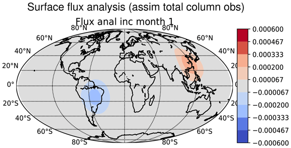
EnviFlux (v1.0): a simplified surface flux inversion tool based on four-dimensional variational data assimilation (4D-Var)

This paper introduces EnviFlux, which is a software tool (written in C++) to study the inverse problem of estimating the distribution of fluxes of a trace gas globally at the Earth's surface. This is done using a four-dimensional variational technique, which combines information from (i) synthetic observations of the trace gas spanning a defined time window, (ii) a transport model linking the initial concentration and surface fluxes to predictions of the observations, and (iii) a priori information. The novelty of this system – compared to those that attempt to solve for real data – is in its relative simplicity and low cost, allowing new ideas to be assessed and understood quickly and cheaply. This is in line with many other developments in data assimilation that are often first explored using so-called “toy” systems. Part of this paper is to document this system, which is sufficiently complex to allow assimilation of in situ and total column amount (TCA) observation in arbitrary configurations, and has a flexible background error covariance model, but is simple enough to be run relatively quickly.

Another part of this paper uses EnviFlux to explore the effect of model error and observation bias on inferred surface fluxes in two example scenarios and with two observation types, namely surface in situ (SIS) and TCA. The first is a highly idealised case with a flux pair (a localised source and a localised sink), where no a priori information concerning their positions is provided. It is found that model errors in the assimilation can severely affect the inferred flux positions and amounts, but observation biases do not affect the positions, but do affect the amounts. The second scenario is closer to a real-world example of methane flux estimates where an a priori is refined with observations. The effect of model error is less than for the first scenario, but is still evident, and the observation biases affect the flux amounts. In both cases, the SIS observations allow a more accurate estimate of surface flux characteristics than the TCA observations, even though the experiments are setup to allow a fair comparison of the two. The last part of the paper raises some research questions that EnviFlux could help address.

1 Introduction

A great potential of data assimilation is in its scope to infer hidden information that cannot be easily measured directly or accurately. The estimation of the rates of exchange of trace gases at the Earth's surface is one example that has important uses, e.g. in understanding and quantifying what processes and locations are responsible for the increasing concentrations of greenhouse gases in the Earth's atmosphere. Example studies include those for carbon dioxide (CO₂) (Chevallier et al., 2005b; Feng et al., 2009), methane (CH₄) (Fraser et al., 2013; Qu et al., 2021), nitrous oxide (N₂O) (Hirsch et al., 2006; Thompson et al., 2019), and other trace gases (Jiang et al., 2013; An et al., 2012; Ma et al., 2021; Palmer et al., 2006; Gonzi et al., 2011). The method works by combining measurements of trace gas concentrations downstream of surface sources or sinks, with rules about how the air gets modified by the sources and sinks, and then how it is transported to the observation sites (this is usually in the form of a chemical transport model). This process is called “inverse modelling” or “top-down flux estimation” (Houweling et al., 2017) and has been applied using a number of techniques. These include direct inversions (using an explicit estimator formula) to infer the fluxes over a small number of large geographical regions (Gurney et al., 2002; Chandra et al., 2022), Markov chain Monte-Carlo (Lunt et al., 2019), regressions (Palmer et al., 2003), back-trajectories (An et al., 2012), fixed-lag Kalman smoothers (Zhuravlev et al., 2013), ensemble Kalman filters (Feng et al., 2009; Bisht et al., 2023; Pendergrass et al., 2023), and four-dimensional variational data assimilation (4D-Var) (Houweling et al., 1999; Chevallier et al., 2005b; Meirink et al., 2008b; Wilson et al., 2014).

Even the most carefully implemented inverse modelling studies have shortcomings owing to unknown or imperfectly modelled processes, unaccounted for errors, or incorrectly specified error covariances. One such issue is the influence of inevitable transport errors on the flux estimates, which has been the subject of numerous studies (Chevallier et al., 2010; Basu et al., 2018; Schuh et al., 2019; Munassar et al., 2023). In particular, Houweling et al. (2010) found that transport errors contributed to the uncertainty in CO₂ fluxes of $\mathrm{0.1}\mathrm{Pg}\mathrm{C}{\mathrm{yr}}^{-\mathrm{1}}({\mathrm{10}}^{\mathrm{6}}{\mathrm{km}}^{\mathrm{2}}{)}^{-\mathrm{1}}$ over land even though the model imperfections resulted in errors in predicted CO₂ column averages of just 0.5 ppm (comparable to the measurement error considered). Jiang et al. (2013) reported that for the estimate of carbon monoxide (CO) fluxes, transport model errors can contribute to 5 % of global emission errors, with larger values as the scale of interest gets smaller, becoming one and a half times the a priori fluxes at the model grid level. Further, Chen et al. (2019) found different locations of CO₂ fluxes depending on the transport model used in the inversion. Another issue is the presence of biases (Chevallier et al., 2005a, 2010), which – whether in the model or in the observations – can contribute to large innovations, and hence to anomalous inferred fluxes.

These, and many other issues (see, e.g. the conclusions section of this paper), means that there is still a huge amount of research to be done to develop and refine inverse modelling techniques. Chemical transport models (CTM, and hence the whole inverse modelling procedures) are expensive to run (Agustí-Panareda et al., 2019), and so there is scope to explore some new ideas using low-cost simplified flux inversion systems that can be run repeatedly without the need for expensive high performance computers. This paper introduces a much simplified Environmental Flux inverse system “EnviFlux” that can be used to do low-cost experimentation around ideas related to such inverse problems. The software is designed to investigate the 4D-Var method of solving the the global flux inversion problem inexpensively by running idealised twin experiments (as other authors have done in more complex and expensive systems, e.g. Chevallier et al., 2007; Basu et al., 2018; Yu et al., 2021; Voshtani et al., 2023. It is hoped that some lessons learned with this simplified system can be transferred to real-world (particularly 4D-Var-based) systems such as those used in Henze et al. (2007) (based on GEOS-Chem, Bey et al., 2001), Chevallier et al. (2005b) (based on LMDZ, Hourdin and Armengaud, 1999), Meirink et al. (2008b) (based on TM5, Krol et al., 2005), Wilson et al. (2014) (INVICAT, based on TOMCAT, Chipperfield, 2006), Hu et al. (2023) (based on WRF-Chem, Grell et al., 2005), and other models, and their developments. This paper demonstrates some findings from EnviFlux by studying the impact of model error and observation biases on the ability to infer the positions and magnitudes of surface fluxes of a generic trace gas.

The structure of this paper is as follows. Section 2 describes the basic set-up of the system, including the state vector, the computational grids, and the tracer transport scheme. Section 3 describes how the inverse problem is solved in the context of 4D-Var. Sections 4 and 5 provide demonstrations of the system, one with a example to estimate the position and magnitude of a source/sink pair in a “weakly Bayesian” (minimal a priori information) context, and another with a more conventional Bayesian set-up to improve a given a priori with observations. Section 6 summarises the findings, and poses some further issues that EnviFlux may be used to study. Appendices A–C describe the formulation, use, and calibration of the spectral-based scheme used for the background error covariance matrix, which comprises a significant part of the system. Appendix D describes the way the software is structured, including the core code (written in C++), and visualisation/post-processing tools (written in python). Appendix E assesses the computational resources needed to run the software, Appendix F shows how the 4D-Var cost function converges with the iteration, and Appendix G discusses some consequences of the model error scheme used. EnviFlux also has a user guide, which complements this paper with some algorithmic details and instructions to run the software. The user guide and code are available in the GitHub repository (Bannister, 2026b), and data are also available (Bannister, 2026a).

2 Description of the system and the forward problem

EnviFlux has many components that work together to estimate the global surface fluxes. This section is a scientific description of the basic components that comprise the forward part of the system. Some finer details are documented in the user guide.

2.1 The continuous equations of motion

The continuous equation of motion for the tracer, χ (a mixing ratio), in 3D is nominally

$$\begin{array}{ll}{\displaystyle \frac{\partial \mathit{\chi }\left(t\right)}{\partial t}}+\mathit{u}\left(t\right)\cdot \mathrm{\nabla }\mathit{\chi }\left(t\right)=& {\displaystyle }\mathbf{S}\mathit{\rho }\left(t\right)+{\mathit{\kappa }}_{\mathrm{h}}{\mathrm{\nabla }}_{\mathrm{h}}^{\mathrm{2}}\mathit{\chi }\left(t\right)\\ \text{(1)}& {\displaystyle }& {\displaystyle }+{\mathit{\kappa }}_{\mathrm{v}}{\displaystyle \frac{{\partial }^{\mathrm{2}}\mathit{\chi }\left(t\right)}{\partial z^{\mathrm{2}}}},\end{array}$$

where u is the prescribed 3D wind vector ($\mathit{u}={\left(\begin{array}{ccc}u& v& w\end{array}\right)}^{⊺}$), ρ is the 2D surface flux field, the operator Sρ constructs a 3D field of zero apart from the surface where it assigns the value $\mathit{\rho }/\left(\mathrm{\Delta }{z}_{\mathrm{0}}{d}_{\mathrm{0}}\right)$ (surface layer thickness Δz₀, surface air density $d_{\mathrm{0}}=\mathrm{1.225}\mathrm{kg}{\mathrm{m}}^{-\mathrm{3}}$), κ_h and κ_v are the horizontal and vertical diffusion coefficients, ∇ is the 3D gradient operator, and ${\mathrm{\nabla }}_{\mathrm{h}}^{\mathrm{2}}$ and ${\partial }^{\mathrm{2}}/\partial z^{\mathrm{2}}$ are the horizontal and vertical Laplacian operators. In practice, Eq. (1) is solved on a discrete grid in space and time (see below). In EnviFlux, χ has units of µg kg⁻¹ (although the units in many applications is moles per mole of dry air), and ρ has units of $\mathrm{\mu }\mathrm{g}{\mathrm{m}}^{-\mathrm{2}}{\mathrm{s}}^{-\mathrm{1}}$. Since the purpose of this work is to study the inverse problem in its simplest form, the tracer in Eq. (1) has no sub-grid influences, like convection and turbulence, nor chemical reactions that would apply to methane e.g. like hydroxyl or photochemical oxidation. Stable tracers like carbon dioxide or sulphur hexafluoride would be the most suitable species for EnviFlux, but this paper focuses on a hypothetical tracer (although in the second example application shown in this paper, Sect. 5, the tracer has a methane-like flux pattern).

2.2 The state vector, the spatial grid, and time-stepping

The core component of EnviFlux is the state vector, x, which comprises the initial and boundary conditions needed to make predictions of the atmospheric tracer mixing ratio, χ(t). The state vector is written

$$\begin{array}{}\text{(2)}& {\displaystyle }{\displaystyle }\mathit{x}=\left(\begin{array}{c}\mathit{\chi }\left(\mathrm{0}\right)\\ \mathit{\rho }\left(\mathrm{0}\right)\\ \mathit{\rho }\left({\mathit{\tau }}_{\mathit{\rho }}\right)\\ \mathrm{⋮}\\ \mathit{\rho }\left(T{\mathit{\tau }}_{\mathit{\rho }}\right)\end{array}\right),\end{array}$$

where χ(0) is the initial 3D tracer field, and ρ(nτ_ρ) is the surface flux field at a set of equally spaced time-steps $n=\mathrm{0},\mathrm{1},\mathrm{\dots },T$ with τ_ρ the time interval between flux fields. Bold symbols indicate the variables are part of the state vector. In this paper sometimes only the χ(0) part of x is referred to and other times only the $\mathit{\rho }\left(\mathrm{0}\right),\mathrm{\dots },\mathit{\rho }\left(T{\mathit{\tau }}_{\mathit{\rho }}\right)$ part. The notation {x}_χ and {x}_ρ shall refer to these parts respectively.

The spatial grid is shown in Fig. 1, which has n_x longitudes, n_y latitudes, and n_z vertical levels. The time-stepping is done in three stages, namely (i) the semi-Lagrangian (SL) advection stage, (ii) the diffusion stage, and (iii) the flux stage, which are described below. EnviFlux uses four kinds of time step, which are as follows (see Fig. 2).

• The minor time step, δt, is the interval used to divide up the back-trajectory for the solver needed for the SL advection scheme.

• The diffusion time step, τ_κ, is the time step used to solve the diffusion part of Eq. (1).

• The major time step, Δt, is the interval between the files specifying u. It is also used as the length of time of each back-trajectory, which is divided into $\mathrm{\Delta }t/\mathit{\delta }t$ sub intervals.

• The flux time step, τ_ρ (mentioned above), is the time interval between flux fields.

The values of these steps are restricted such that $\mathrm{\Delta }t/\mathit{\delta }t$, $\mathrm{\Delta }t/{\mathit{\tau }}_{\mathit{\kappa }}$, and ${\mathit{\tau }}_{\mathit{\rho }}/\mathrm{\Delta }t$ are positive integers. The three stages of the model's time-stepping (over a major time step, Δt) are as follows.

1. The first stage solves the advection part of Eq. (1) with the SL method. Each χ point on the grid is taken as a “starting point” in a back trajectory calculation from time t back to t−Δt. This time is divided into smaller steps of size δt where the backward path for each is calculated using fourth-order Runge–Kutta (Press et al., 2007). This leads to an “end point” at t−Δt for each trajectory. The “start” and “end” are in inverted commas as a reminder that these are meant in a backward time sense. The value of χ at the “starting point” at time t after this first stage is replaced by the value of χ at the “end point” at t−Δt. This involves spatial interpolation. EnviFlux allows tri-linear or tri-cubic interpolation, with the latter recommended to reduce loss of conservation. Advection is driven by prescribed 3D wind fields, stored in an archive of files; in this paper these are derived from the Eurpoean Reanalysis 5 (ERA-5) winds (Hersbach et al., 2020). As the forward model (and the adjoint) is repeated many times during an assimilation (Sect. 3), the “end points” are archived so the trajectories do not need to be computed each time. We call this “boosting” as it speeds up the computation.

2. The second stage solves the diffusion part of Eq. (1). Practically, the advected field from stage 1 is copied back to t−Δt and a pure diffusion equation (Eq. 1 without the advection and flux terms) is integrated using standard finite-differences with steps of size τ_κ to time t. Diffusion can be applied as a physical process, or to stablise a numerical scheme. For the experiments shown in this paper, no explicit diffusion is applied as the SL scheme is stable and introduces its own numerical diffusion.

3. The third stage introduces the surface fluxes to the model's layer closest to the surface with an increment of $\mathit{\rho }\times \mathrm{\Delta }t/\left(d_{\mathrm{0}}\mathrm{\Delta }{z}_{\mathrm{0}}\right)$, where d₀ and Δz₀ are defined above. This form assumes that the fluxes add tracer to or remove tracer from the air uniformly within the surface grid layer at each horizontal position. The particular flux field time in the state vector (Eq. 2) used in this step is simply $\text{int}(t/{\mathit{\tau }}_{\mathit{\rho }})$, where the int(•) function rounds down to the nearest integer. In other words ρ(nτ_ρ) is the flux field valid between times $n{\mathit{\tau }}_{\mathit{\rho }}\le t<(n+\mathrm{1}){\mathit{\tau }}_{\mathit{\rho }}$.

The output of the third stage approximates the solution of Eq. (1) at time t. The approximations made in these steps are assumed to be adequate for this simplified system. As stated above, EnviFlux does not include (sub-grid) turbulent or convective transport processes, nor chemical reactions.

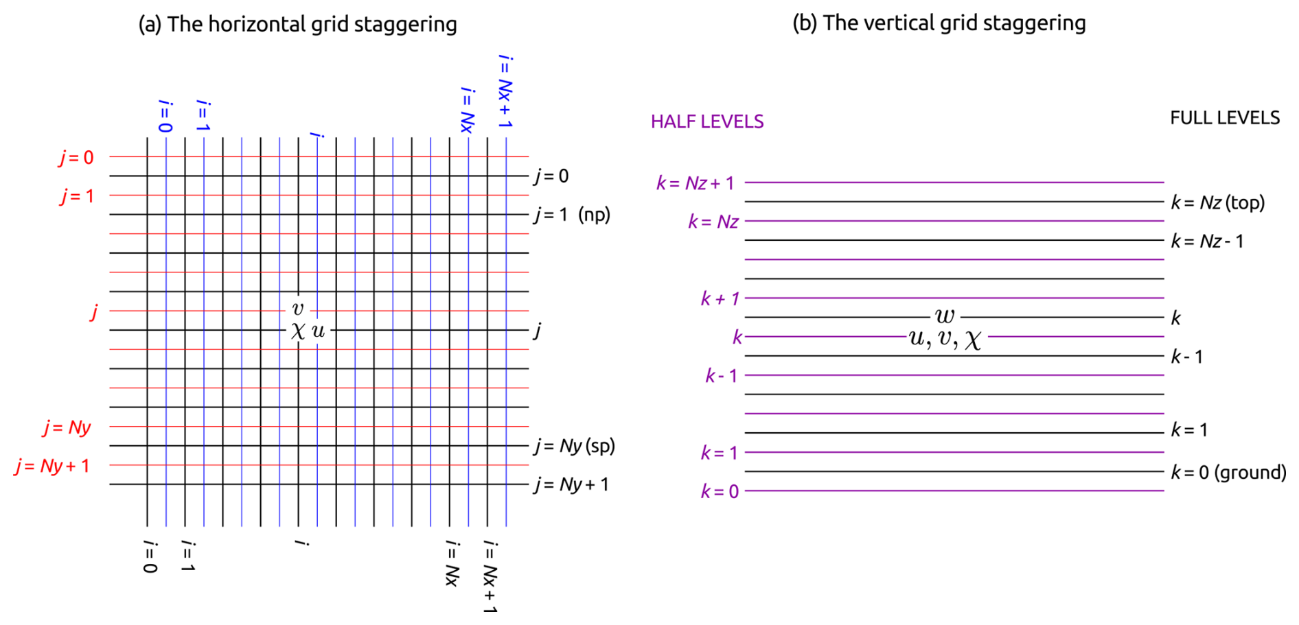
Figure 1 The horizontal (a) and vertical (b) model grids used for EnviFlux. In the horizontal, the tracer (χ), flux (ρ), and vertical wind (w) are stored at points where the black lines cross and indexed with the black i and j. The zonal wind (u) is stored at intermediate longitudes indexed with the blue i, and at the same latitudes as χ. The meridional wind (v) is stored at the same longitudes as χ, and intermediate latitudes indexed with the red j. The north (np) and south (sp) poles lie on black latitudes. This is the Arakawa “C” grid. In EnviFlux the longitudes are equally spaced, but the latitudes are Gaussian latitudes, which are not equally spaced (this is to allow accurate application of a spherical transform used to model the B-matrix – see Sect. 3.3). In the vertical, χ, u, and v are stored on “half levels” indexed with the purple k, and w is stored on “full levels” indexed with the black k. This is the Charney–Phillips staggering.

Figure 2 Timeline showing the time-stepping schemes used by EnviFlux, showing the four time intervals used. The back trajectories used for the semi-Lagrangian advection are of time length Δt, which are comprised of minor time-steps, δt. Δt is also the time interval of the wind files. Explicit diffusion effects are introduced with a timestep τ_κ, and the flux fields have a time interval of τ_ρ.

For the rest of this paper, we shall represent these three steps with the linear propagator $\mathit{\chi }\left(k\mathrm{\Delta }t\right)={\mathbf{M}}_{k-\mathrm{1}\to k}^{{\left\{\mathit{x}\right\}}_{\mathit{\rho }}}\mathit{\chi }\left([k-\mathrm{1}]\mathrm{\Delta }t\right)$, where the {x}_ρ superscript indicates that the propagator is dependent on the surface flux part of the state vector, Eq. (2), which obviously influences the model trajectory. The surface flux does not get updated, which is why it is not part of the main argument. There are three caveats about the meaning of this propagator. The first is that when $k-\mathrm{1}=\mathrm{0}$ the argument of ${\mathbf{M}}_{k-\mathrm{1}\to k}^{{\left\{\mathit{x}\right\}}_{\mathit{\rho }}}$, i.e. χ(0), must be identical to the tracer component of the state vector, i.e. {x}_χ. The propagator definition may therefore be refined:

$$\begin{array}{}\text{(3)}& {\displaystyle }{\displaystyle }\mathit{\chi }\left(k\mathrm{\Delta }t\right)=\left\{\begin{array}{ll}{\mathbf{M}}_{k-\mathrm{1}\to k}^{{\left\{\mathit{x}\right\}}_{\mathit{\rho }}}\mathit{\chi }\left([k-\mathrm{1}]\mathrm{\Delta }t\right)& k-\mathrm{1}>\mathrm{0}\\ {\mathbf{M}}_{k-\mathrm{1}\to k}^{{\left\{\mathit{x}\right\}}_{\mathit{\rho }}}{\left\{\mathit{x}\right\}}_{\mathit{\chi }}& k-\mathrm{1}=\mathrm{0}.\end{array}\right.\end{array}$$

The second and third caveats are covered in the next section.

2.3 The adjoint step

The second caveat concerns the adjoint operator, i.e. $\widehat{\mathit{\chi }}\left([k-\mathrm{1}]\mathrm{\Delta }t\right):={\left({\mathbf{M}}_{k-\mathrm{1}\to k}^{{\left\{\widehat{\mathit{x}}\right\}}_{\mathit{\rho }}}\right)}^{⊺}\widehat{\mathit{\chi }}\left(k\mathrm{\Delta }t\right)$. The action of the adjoint propagates gradient¹ information (indicated with the hat) from $\widehat{\mathit{\chi }}\left(k\mathrm{\Delta }t\right)$ backwards in time to $\widehat{\mathit{\chi }}\left([k-\mathrm{1}]\mathrm{\Delta }t\right)$. Additionally, this operator must incrementally update the gradient state ${\left\{\widehat{\mathit{x}}\right\}}_{\mathit{\rho }}$. The third caveat concerns the action of the adjoint at the earliest time. While when $t-\mathrm{\Delta }t>\mathrm{0}$, the output of the adjoint operator is the tracer gradient, $\widehat{\mathit{\chi }}\left([k-\mathrm{1}]\mathrm{\Delta }t\right)$ (and update of ${\left\{\widehat{\mathit{x}}\right\}}_{\mathit{\rho }}$), as indicated above, in the special case when $k-\mathrm{1}=\mathrm{0}$, i.e. ${\left({\mathbf{M}}_{\mathrm{0}\to \mathrm{1}}^{{\left\{\widehat{\mathit{x}}\right\}}_{\mathit{\rho }}}\right)}^{⊺}$, the output will be defined as the gradient of the whole state vector. In summary:

$$\begin{array}{}\text{(4)}& {\displaystyle }{\displaystyle }{\left({\mathbf{M}}_{k-\mathrm{1}\to k}^{{\left\{\widehat{\mathit{x}}\right\}}_{\mathit{\rho }}}\right)}^{⊺}\widehat{\mathit{\chi }}\left(k\mathrm{\Delta }t\right):=\left\{\begin{array}{ll}\widehat{\mathit{\chi }}\left([k-\mathrm{1}]\mathrm{\Delta }t\right)& k>\mathrm{1}\\ \left(\begin{array}{c}\widehat{\mathit{\chi }}\left(\mathrm{0}\right)\\ \widehat{\mathit{\rho }}\left(\mathrm{0}\right)\\ \widehat{\mathit{\rho }}\left({\mathit{\tau }}_{\mathit{\rho }}\right)\\ \mathrm{⋮}\\ \widehat{\mathit{\rho }}\left(T{\mathit{\tau }}_{\mathit{\rho }}\right)\end{array}\right)& k=\mathrm{1},\end{array}\right.\end{array}$$

where the $\widehat{\mathit{\rho }}$ are the accumulations of increments held in the ${\left\{\widehat{\mathit{x}}\right\}}_{\mathit{\rho }}$ superscript during the course of the adjoint operations (as mentioned in caveat 2). This definition is for notational convenience when computing the gradient of the cost function (see Sect. 3.1).

3 Description of the inverse problem

This section is a description of how the surface fluxes are inferred from observations.

3.1 The cost function

EnviFlux uses an incremental formulation of the cost function that is minimised during the 4D-Var. In this formulation, $\mathit{x}={\mathit{x}}^{\mathrm{b}}+\mathit{\delta }\mathit{x}$, where x^b is the background field (a priori), and δx is the increment, found by minimising the 4D-Var cost function. Instead of varying δx directly, a control variable, δv is varied, where δx and δv are related via δx=B^½δv, where B is the background error covariance matrix (Sect. 3.3). This change of variable removes the B-matrix in explicit form from the cost function, and helps improve the conditioning (see e.g. Bannister, 2008b or Sect. 3.1 of Bannister, 2026b). In terms of δv the cost function is

$$\begin{array}{ll}{\displaystyle }& {\displaystyle }{J}_{\mathit{\delta }\mathit{v}}\left(\mathit{\delta }\mathit{v}\right)={\displaystyle \frac{\mathrm{1}}{\mathrm{2}}}\mathit{\delta }{\mathit{v}}^{⊺}\mathit{\delta }\mathit{v}\\ {\displaystyle }& {\displaystyle }+{\displaystyle \frac{\mathrm{1}}{\mathrm{2}}}\sum _{k=\mathrm{0}}^{N_T}{\left({\mathit{y}}_k-{\mathbf{H}}_k{\mathbf{M}}_{\mathrm{0}\to k}^{{\left\{{\mathit{x}}^{\mathrm{b}}+{\mathbf{B}}^{\frac{\mathrm{1}}{\mathrm{2}}}\mathit{\delta }\mathit{v}\right\}}_{\mathit{\rho }}}\left[{\mathit{\chi }}^{\mathrm{b}}\left(\mathrm{0}\right)+{\left\{{\mathbf{B}}^{\frac{\mathrm{1}}{\mathrm{2}}}\mathit{\delta }\mathit{v}\right\}}_{\mathit{\chi }}\right]\right)}^{⊺}\\ \text{(5)}& {\displaystyle }& {\displaystyle }\times {\mathbf{R}}_k^{-\mathrm{1}}\left(•\right),\end{array}$$

where the notation {x}_χ and {x}_ρ is explained in Sect. 2.2, N_T is the number of major time-steps in the problem, y_k is the set of observations made at time-step k, H_k is the observation operator, R_k is the observation error covariance matrix, and ${\mathit{\chi }}^{\mathrm{b}}\left(\mathrm{0}\right)={\left\{{\mathit{x}}^{\mathrm{b}}\right\}}_{\mathit{\chi }}$ is the background tracer at t=0. The “${\mathit{a}}^{⊺}{\mathbf{A}}^{-\mathrm{1}}•$” notation is shorthand for “${\mathit{a}}^{⊺}{\mathbf{A}}^{-\mathrm{1}}\mathit{a}$”, for brevity. Even though the notation in Eq. (5) implies that observations are at major time-steps only, EnviFlux does allow observations to be made at intermediate times, which are treated with linear interpolation (for details see Sect. 3.2.1 of Bannister, 2026b).

The gradient of the cost function is

$$\begin{array}{ll}{\displaystyle }& {\displaystyle }{\mathrm{\nabla }}_{\mathit{\delta }\mathit{v}}J\left(\mathit{\delta }\mathit{v}\right)=\mathit{\delta }\mathit{v}\\ {\displaystyle }& {\displaystyle }-{\mathbf{B}}^{\frac{⊺}{\mathrm{2}}}\sum _{k=\mathrm{0}}^{N_T}{\left({\mathbf{M}}_{\mathrm{0}\to k}^{{\left\{{\mathit{x}}^{\mathrm{b}}+{\mathbf{B}}^{\frac{\mathrm{1}}{\mathrm{2}}}\mathit{\delta }\mathit{v}\right\}}_{\mathit{\rho }}}\right)}^{⊺}{\mathbf{H}}_k^{⊺}{\mathbf{R}}_k^{-\mathrm{1}}\\ \text{(6)}& {\displaystyle }& {\displaystyle }\times \left({\mathit{y}}_k-{\mathbf{H}}_k{\mathbf{M}}_{\mathrm{0}\to k}^{{\left\{{\mathit{x}}^{\mathrm{b}}+{\mathbf{B}}^{\frac{\mathrm{1}}{\mathrm{2}}}\mathit{\delta }\mathit{v}\right\}}_{\mathit{\rho }}}\left[{\mathit{\chi }}^{\mathrm{b}}\left(\mathrm{0}\right)+{\left\{{\mathbf{B}}^{\frac{\mathrm{1}}{\mathrm{2}}}\mathit{\delta }\mathit{v}\right\}}_{\mathit{\chi }}\right]\right),\end{array}$$

where ${\mathbf{B}}^{\frac{⊺}{\mathrm{2}}}={\left({\mathbf{B}}^{\frac{\mathrm{1}}{\mathrm{2}}}\right)}^{⊺}$, which is fed to a conjugate gradient-based descent algorithm (Golub and Van Loan, 1996; Lewis et al., 2006) to iteratively minimise the cost function. A version of the gradient calculation that is more efficient to compute than Eq. (6) is used by EnviFlux (see Sect. 3.2.2 of Bannister, 2026b).

The block partitioning of δv is similar to that of x in Eq. (2) in the sense that the first part concerns the initial conditions and the remainder concerns the surface fluxes:

$$\begin{array}{}\text{(7)}& {\displaystyle }{\displaystyle }\mathit{\delta }\mathit{v}=\left(\begin{array}{c}\text{initial conditions}\\ \\ \text{surface fluxes}\\ \end{array}\right).\end{array}$$

The size of each block in δv is the same as in x, but the elements have different meanings. The elements represent weights of different spectral components, and vertical or temporal modes. This is discussed further in Sect. 3.3.

3.2 Observations and observation operators

EnviFlux allows three types of observation to be assimilated, namely in situ tracer observations, integrated total column amount (TCA) observations, and direct flux observations. Observations can be at any geographical location, and tracer observations can additionally be made at any height above the surface within the domain. The model's version of the observations, H_kχ(kΔt), are found by linear interpolation in space and time. The TCA observations are found from a discretisation of the vertical integral ∫χ(z)d_zdz, where z is height above the surface, d_z is the air density (this has a similar mathematical structure as the Jacobian of the radiative transfer models used to assimilate some satellite observations), and χ(z) is the tracer field interpolated to the geographical location and time of each observation.

Currently in EnviFlux, observation errors are assumed uncorrelated. The observation error standard deviations, σ^o, can be set arbitrarily for each observation, and the diagonal elements of the R-matrix is made up of values ${{\mathit{\sigma }}^{\mathrm{o}}}^{\mathrm{2}}$. EnviFlux uses these observation operators in the assimilation, and the same operators are used to make synthetic observations as part of the twin experiment method.

3.3 The background error covariance matrix

The background error covariance matrix, or B for short, is a fundamental component of a Gaussian-based Bayesian problem, such as that described by Eq. (5). As in most assimilation systems, the probability density function of background errors is assumed to be Gaussian, where the mean is x^b and the error covariance is B. The B-matrix specifies, statistically, how large background errors are and how background errors are correlated, e.g. Bannister (2008a). The background term of the unprecondioned cost function – when written in terms of δx, see Eq. (6) of Bannister (2026b) – is proportional to minus the logarithm of this PDF.

In the preconditioned cost function, Eq. (5), the new variable, δv, is chosen to have unit background error covariances, which means that the background errors in this δv-representation are uncorrelated and have unit variance. The B-matrix appears in this preconditioned system via a square-root in the variable transform B^½, i.e. δx=B^½δv (for more details about this kind of variable transform, see e.g. Bannister, 2008b or Bannister, 2020). B^½ is a large matrix, and so instead of storing it explicitly, it is formulated with a set of component operators, called a background error covariance model. In practice these are compactly encoded as subroutines. In EnviFlux it has the following form:

$$\begin{array}{}\text{(8)}& {\displaystyle }{\displaystyle }{\mathbf{B}}^{\frac{\mathrm{1}}{\mathrm{2}}}=\left(\begin{array}{ccc}{\mathbf{\Sigma }}_{\mathit{\chi }}^{\mathrm{b}}{\mathbf{F}}_{\mathrm{v}\mathit{\chi }}{\mathbf{\Lambda }}_{\mathrm{v}\mathit{\chi }}^{\frac{\mathrm{1}}{\mathrm{2}}}{\mathbf{F}}_{\mathrm{v}\mathit{\chi }}^{⊺}{\mathbf{R}}_{\mathrm{h}}{\mathbf{S}}_{\mathrm{h}}{\mathbf{\Lambda }}_{\mathrm{h}\mathit{\chi }}^{\frac{\mathrm{1}}{\mathrm{2}}}& |& \mathbf{0}\\ & |\\ \mathbf{0}& |& {\mathbf{\Sigma }}_{\mathit{\rho }}^{\mathrm{b}}{\mathbf{F}}_{\mathrm{t}\mathit{\rho }}{\mathbf{\Lambda }}_{\mathrm{t}\mathit{\rho }}^{\frac{\mathrm{1}}{\mathrm{2}}}{\mathbf{F}}_{\mathrm{t}\mathit{\rho }}^{⊺}{\mathbf{R}}_{\mathrm{h}}{\mathbf{S}}_{\mathrm{h}}{\mathbf{\Lambda }}_{\mathrm{h}\mathit{\rho }}^{\frac{\mathrm{1}}{\mathrm{2}}}\\ & |\end{array}\right),\end{array}$$

which acts on δv of the form of Eq. (7). The top-left block operates on the initial condition part of δv and the bottom-right block operates on the flux part of δv, and there is no coupling between them in this choice of model. Alternative B-matrix models may be coded instead, but the parts of this B^½, associated with the initial conditions and fluxes, are now explained in turn.

3.3.1 The part of B^½ associated with the initial conditions

The first part of B^½ is associated with the initial conditions, χ(0) (upper left in Eq. 8).

1. In the order of operation, the first stage (${\mathbf{S}}_{\mathrm{h}}{\mathbf{\Lambda }}_{\mathrm{h}\mathit{\chi }}^{\frac{\mathrm{1}}{\mathrm{2}}}$) models horizontal correlations of χ(0). Suppose that horizontal correlations are represented by the matrix C_hχ. This can be written in its eigenvalue decomposition ${\mathbf{C}}_{\mathrm{h}\mathit{\chi }}={\mathbf{S}}_{\mathrm{h}}{\mathbf{\Lambda }}_{\mathrm{h}\mathit{\chi }}{\mathbf{S}}_{\mathrm{h}}^{⊺}$, where Λ_hχ is the (diagonal) matrix of eigenvalues, and S_h is the matrix of eigenvectors. This form justifies this particular square-root, ${\mathbf{S}}_{\mathrm{h}}{\mathbf{\Lambda }}_{\mathrm{h}\mathit{\chi }}^{\frac{\mathrm{1}}{\mathrm{2}}}$ (so that the square-root multiplied by its transpose gives C_hχ). Here, S_h is chosen to be a spherical spectral transform (transforming from a spectral space representation of the control vector to a grid space representation), so the eigenvectors have the assumed form of spherical harmonics. The spectral representation is a grid of wavenumbers ℓ (the “degree” wavenumber), m (the “order” wavenumber) (see Appendix A), and vertical level. The form of the transform is symbolic only, as practically the horizontal transform is applied separately for each vertical level (as a Kronecker product). The diagonals of Λ_hχ are prescribed functions of ℓ, which goes from 0 to the maximum value L (where $n_x=\mathrm{2}L+\mathrm{1}$ and $n_y=L+\mathrm{1}$) and we use the same function for each vertical level. The shape of Λ_hχ sets the horizontal lengthscale for initial tracer background errors. S_h uses the SHTools software (Wieczorek et al., 2018). A tutorial on this horizontal transform is given in Appendix A, how it is applied in Appendix B1, and how Λ_hχ is found in Appendix C1. The natural output grid for S_h is a Gaussian grid, and SHTools uses co-latitudes. EnviFlux uses the same Gaussian grid and the reconfiguration R_h operator here just transforms from co-latitudes to geographical latitudes.

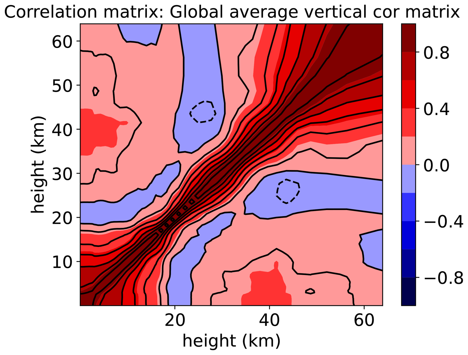
2. The next stage (${\mathbf{F}}_{\mathrm{v}\mathit{\chi }}{\mathbf{\Lambda }}_{\mathrm{v}\mathit{\chi }}^{\frac{\mathrm{1}}{\mathrm{2}}}{\mathbf{F}}_{\mathrm{v}\mathit{\chi }}^{⊺}$), models vertical correlations. The eigenvector and eigenvalue matrices (F_vχ and Λ_vχ respectively, each n_z×n_z matrices) are derived from the proposed vertical correlation matrix shown in Fig. 3. Again, this transform is symbolic only, as practically the vertical matrices are applied separately for each horizontal position (as a Kronecker product). Practical notes are given in Appendix B2, how F_vχ and Λ_vχ are found is described in Appendix C2.

3. The last matrix, ${\mathbf{\Sigma }}_{\mathit{\chi }}^{\mathrm{b}}$, is a diagonal matrix and specifies how background error standard deviations of the initial tracer depend on position in space. This is discussed in Sect. 3.3.3.

Figure 3 The vertical error correlation matrix for χ(0), which is used to find the eigenvectors, F_vχ, and eigenvalues, Λ_vχ. This matrix is computed according to the procedure outlined in Appendix C2.

3.3.2 The part of B^½ associated with the fluxes

The second part of B^½ is that associated with the surface fluxes, ρ (bottom right in Eq. 8).

• 4.

  The first stage is ${\mathbf{S}}_{\mathrm{h}}{\mathbf{\Lambda }}_{\mathrm{h}\mathit{\rho }}^{\frac{\mathrm{1}}{\mathrm{2}}}$. This is similar to point 1 above and again the form is symbolic only, as practically the transform is applied separately to each of the T+1 flux times. The diagonals of Λ_hρ form a prescribed function of ℓ. The shape of Λ_hρ sets the horizontal lengthscale for flux background errors. See Appendices A, B1, and C1. The R_h operator is the same as in point 1 above.

• 5.

  The next stage is ${\mathbf{F}}_{\mathrm{t}\mathit{\rho }}{\mathbf{\Lambda }}_{\mathrm{t}\mathit{\rho }}^{\frac{\mathrm{1}}{\mathrm{2}}}{\mathbf{F}}_{\mathrm{t}\mathit{\rho }}^{⊺}$, which models temporal correlations for ρ. The temporal eigenvectors, F_tρ, and eigenvalues, Λ_tρ, are derived from a prescribed $(T+\mathrm{1})\times (T+\mathrm{1})$ temporal correlation matrix with a specified correlation timescale. See Appendices B3 and C3.

• 6.

  The last matrix, ${\mathbf{\Sigma }}_{\mathit{\rho }}^{\mathrm{b}}$ (see Sect. 3.3.3), is a diagonal matrix and specifies how background error standard deviations in $\mathit{\rho }\left(\mathrm{0}\right),\mathrm{\dots },\mathit{\rho }\left(T{\mathit{\tau }}_{\mathit{\rho }}\right)$ depend on position in space. ${\mathbf{\Sigma }}_{\mathit{\rho }}^{\mathrm{b}}$ has the following $(T+\mathrm{1})\times (T+\mathrm{1})$ block form:

  $$\begin{array}{}\text{(9)}& {\displaystyle }{\displaystyle }{\mathbf{\Sigma }}_{\mathit{\rho }}^{\mathrm{b}}=\left(\begin{array}{c}{\mathbf{\Sigma }}_{\mathit{\rho }\left(\mathrm{0}\right)}^{\mathrm{b}}\\ & \mathrm{\ddots }\\ & & {\mathbf{\Sigma }}_{\mathit{\rho }\left(T{\mathit{\tau }}_{\mathit{\rho }}\right)}^{\mathrm{b}}\end{array}\right).\end{array}$$

As the χ and ρ parts in B^½ are separate, this assumes that background errors between these are uncorrelated. Including such coupling is beyond the scope of this work.

3.3.3 The background error standard deviations, ${\mathbf{\Sigma }}_{\mathit{\chi }}^{\mathrm{b}}$ and ${\mathbf{\Sigma }}_{\mathit{\rho }}^{\mathrm{b}}$

The background error standard deviation fields (diagonals of ${\mathbf{\Sigma }}_{\mathit{\chi }}^{\mathrm{b}}$ and ${\mathbf{\Sigma }}_{\mathit{\rho }}^{\mathrm{b}}$) influence how much information is provided by the background verses the observations. ${\mathbf{\Sigma }}_{\mathit{\chi }}^{\mathrm{b}}$ is a function of longitude, latitude, and height, and ${\mathbf{\Sigma }}_{\mathit{\rho }}^{\mathrm{b}}$ is a function of longitude, latitude, and time (in time intervals of τ_ρ). Where and when the background error standard deviation is larger, the assimilation has less confidence in the background and so gives more relative weight to the observations. The particular choices of ${\mathbf{\Sigma }}_{\mathit{\chi }}^{\mathrm{b}}$ and ${\mathbf{\Sigma }}_{\mathit{\rho }}^{\mathrm{b}}$ can be chosen arbitrarily.

4 A “weakly Bayesian” example for source/sink location detection

A first, and novel, demonstration is to investigate how well EnviFlux can identify the locations (and “strengths”) of a pair of localised flux features from observations only. The details of these experiments, including the background error covariance specifications and the observation details, are provided in the middle column of Table 1. In particular, the configuration of L=32 ($\mathrm{2}L+\mathrm{1}=\mathrm{65}$ longitudes, $L+\mathrm{1}=\mathrm{33}$ latitudes), and 56 vertical levels is used, with an assimilation window of 100 d (providing time for air parcels to travel continental scales or more) and a 12-h major time-step. Further, fluxes are considered constant for τ_ρ=30 d and have a three-month temporal correlation timescale. This allows fluxes to have a seasonal cycle and change smoothly (although only part of the seasonal cycle is considered here). The 4D-Var is always run with a fixed number of inner loop iterations (25), which we have found adequate for convergence (shown in Appendix F for this and a selection of other experiments in this paper). A guide to the computational resources needed to run EnviFlux is provided in Appendix E. Figure 4 shows the initial conditions and flux field used as the truth for this experiment. The pair of features comprises a source point of peak strength 0.004 $\mathrm{\mu }\mathrm{g}{\mathrm{m}}^{-\mathrm{2}}{\mathrm{s}}^{-\mathrm{1}}$ and a sink point of peak strength 0.005 $\mathrm{\mu }\mathrm{g}{\mathrm{m}}^{-\mathrm{2}}{\mathrm{s}}^{-\mathrm{1}}$. The source location reflects a real-world emission location of methane – see, e.g. Fig. 4 of Qu et al. (2021) – but the sink location is chosen for curiosity only, as in reality methane sinks are not localised in this way.

Table 1 Specifications of the two sets of experiments that are done. The first set is for the feature detection experiments (Sect. 4, middle column) and the second set is for the flux adjustment experiments (Sect. 5, right column). The vector δv is defined as a vector of independent random numbers, each drawn from the Gaussian distribution N(0,1). For each set of experiments, separate total column amount (TCA) and surface in situ (SIS) observations (Sect. 3.2) are assimilated. The geographical locations of the observations follow that of an orbiting satellite. The observation error standard deviations, σ°, are determined by doing a run of the true state over the experimental period, and then taking ∼10 % of the standard deviation of the computed observations.

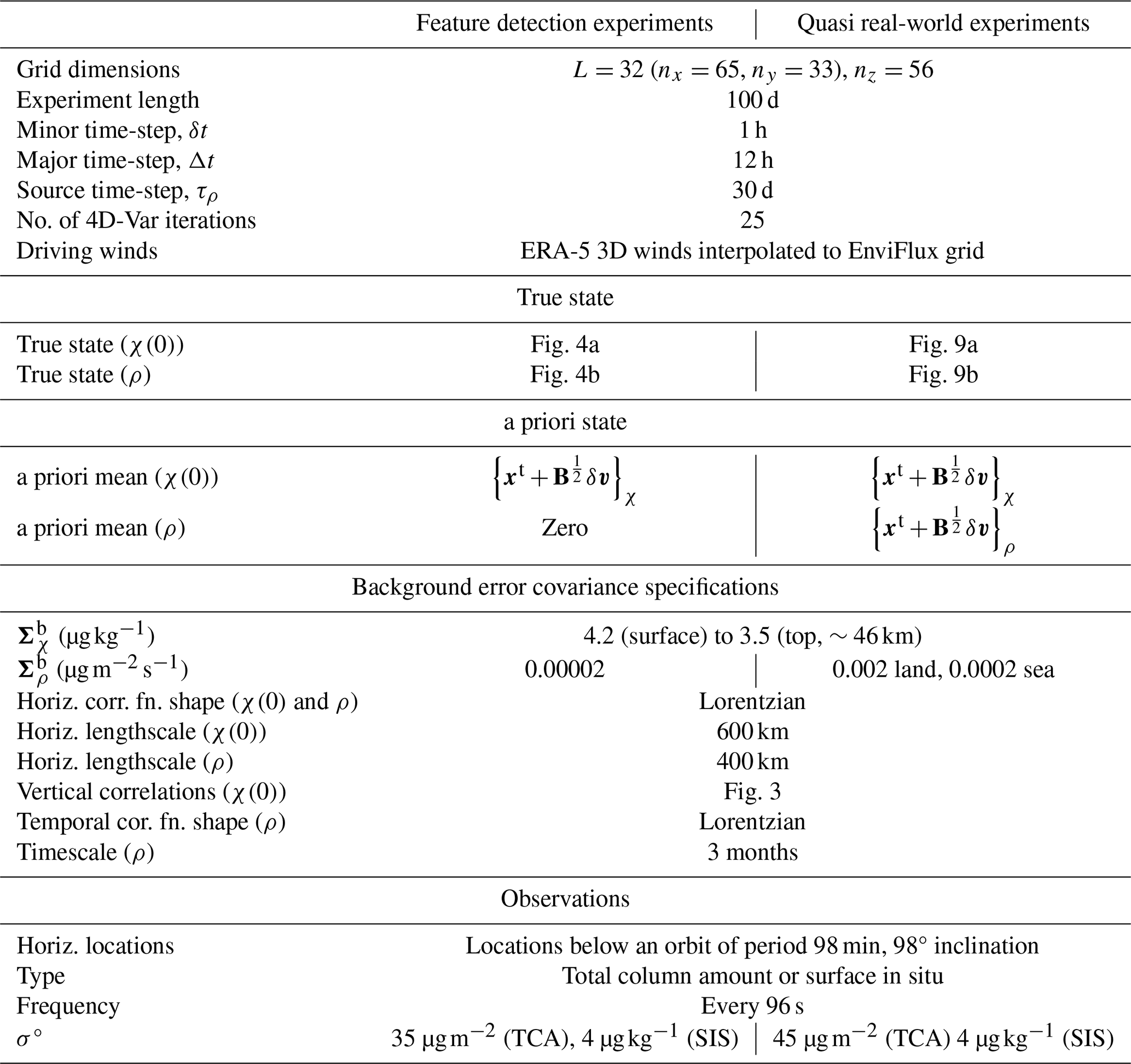
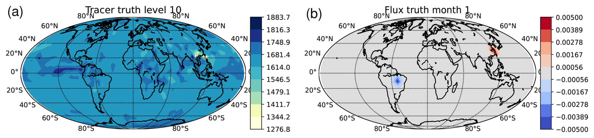
Figure 4 The true state chosen for the source/sink location detection experiments. Panel (a) is for χ^t(0) at level 10 (850 m above the ground, units µg kg⁻¹) and panel (b) is for ρ^t(0) (corresponding to the first 30 d, units $\mathrm{\mu }\mathrm{g}{\mathrm{m}}^{-\mathrm{2}}{\mathrm{s}}^{-\mathrm{1}}$). In (b), red is a source and blue is a sink.

In these experiments, no a priori information about the features' positions is provided. The a priori (background) state for the initial conditions is a perturbed version of the truth found with B^½δv, where δv is a random vector in control space with elements drawn from N(0,1). On the colour scale of Fig. 4a, the perturbed field is barely distinguishable, so is not shown. The a priori state for the flux field is a zero field at each source time-step over the 100 d experiment, meaning that the system has no a priori information about the locations, making this an interesting and challenging test of the inverse problem (something that could happen in a real-world application if sources or sinks appear that are not accounted for in the a priori).

Two kinds of observations are separately assimilated, namely (i) total column amount (TCA) observations following an orbital track (see Table 1 for the details), and (ii) surface in situ (SIS) observations at the same geographical positions. Even though this reflects a realistic observational situation for the TCA observations (such as those made from GOSAT Yokota et al., 2009 allowing for screening), it is not for SIS observations, but we study the SIS observations along the orbital track so the impact of the two observation types can be directly compared. This is a similar design strategy to that used by Basu et al. (2018). Here, each is taken as a point location in the horizontal, even though in reality the remotely-sensed observations can have a footprint of 10 s of km (Yokota et al., 2009) Consequently, there is no need to account for representativess error (Hodyss and Nichols, 2015) here as the observations have been prepared with random error only. Unlike for real-world studies, there is no need here to consider cloud screening.

4.1 Location experiments: “perfectly specified” assimilation results

The posterior (analysis) states that follow from a run of EnviFlux with near perfect specifications (meaning the B-matrix is a near perfect reflection of the actual errors², the R-matrix is a perfect reflection of observation errors, there is no model error, and there are no explicit biases) are shown in Fig. 5. In fact this Fig. shows the analysis increments: these allow the adjustments to the initial conditions to be shown clearly, and, given that the background flux field is zero, the flux increment field is the same as the flux analysis.

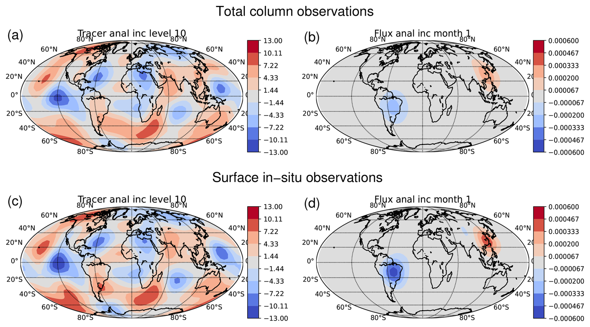
Figure 5 Analysis increments, δχ^a(0) (units µg kg⁻¹) and δρ^a(0) (units $\mathrm{\mu }\mathrm{g}{\mathrm{m}}^{-\mathrm{2}}{\mathrm{s}}^{-\mathrm{1}}$), found by assimilating either TCA (top row) or SIS observations (bottom row) for the near perfect source/sink location detection experiments. Panels (a) and (c) are for δχ^a(0) at level 10, and panels (b) and (d) are for δρ^a(0). These plots should be compared to the true fields in Fig. 4. Red increments are positive and blue increments are negative. When comparing panels (b) and (d) to Fig. 4b, note the different colour scales.

The increments to χ(0) are very similar between the two observation types TCA (a) and SIS (c) and there are no strong peaks/troughs in the increment fields at the two source/sink locations. If there were especially large positive increments at the source location and negative increments at the sink location, it would suggest that the system was treating the systematic lack/excess of tracer at these two respective locations (due to the ρ^b=0) was partly due to errors in χ^b(0). In fact, the analysis increment patterns in χ(0) match those of the chosen background error field, χ^b(0)−χ^t(0) (not shown), but of opposite sign, indicating that the assimilation is doing a good job at adjusting χ^b(0) towards the truth, despite the large errors in ρ^b.

The flux analyses after assimilating the two observation types TCA (b) and SIS (d) show features in the correct places, c.f. Fig. 4b. This shows the ability of inverse modelling systems like EnviFlux to identify locations of fluxes that are not known to the a priori. There are, however, two major issues. One is the over-estimation of the geographical extent of the features and the other is the under-estimation of the peak fluxes (the analyses underestimate the peaks by more than a factor of 10). These findings are perhaps not surprising as an assimilation system naturally smooths-out information (see e.g. arguments about the resolution of inverse problems in Rodgers, 2000), and the assimilation is constraining the flux to be as close to zero as possible to match the prior. These two findings are linked. Arguably it is the area integrated source and sink fields that are important rather than the peak values, so if the analysed flux features are spatially smoothed, the peak values need to be reduced to keep the area integrated values stable. We found by trial-and-error that the relatively small value of ${\mathbf{\Sigma }}_{\mathit{\rho }}^{\mathrm{b}}=\mathrm{0.00002}\mathrm{\mu }\mathrm{g}{\mathrm{m}}^{-\mathrm{2}}{\mathrm{s}}^{-\mathrm{1}}$ (see Table 1) keeps the integrated source and integrated sink values close to the true equivalents for the SIS observation system. Incidentally, significantly increasing the value of ${\mathbf{\Sigma }}_{\mathit{\rho }}^{\mathrm{b}}$ increases the analysed peak flux analysis values only marginally (not shown), supporting the argument that the assimilation constrains the integrated flux values more strongly than the specific peak values. This issue is studied more in the context of model error and observation bias in Sect. 4.3.

Interestingly, we find that TCA observations constrain the fluxes to a lesser degree than the SIS data can, despite the observing systems being set-up to have similar information coming from each (in the sense that the numbers of observations are the same and choosing σ^o values of the same percentage (10 %) of the respective variabilities of the model's equivalents, see Table 1). This is an understandable result as a significant part of the TCA measurements originates away from the surface.

4.2 Location experiments: effect of model error

We now study the effect of model error on the results. It is already known that transport uncertainties in the assimilation can influence the position and strength of sources, Yu et al. (2021), and we study this using the simple source/sink pair set-up. There are a number of ways of simulating model transport error, but it is simulated here by multiplying the vertical wind, w, in the assimilation by a number, η, close to unity (0.9 and 1.1), while the observations assimilated are still generated from samples from a run using the true winds (actually they are identical to those experiments in Sect. 4.1). Changing the vertical winds, but keeping the same horizontal winds, will not directly affect how the tracer is circulated around the globe, although there will be an indirect consequence, e.g. by affecting which levels (including jet levels) the tracer can reach. Maintaining the true horizontal winds though means that the tracer still has the same potential to reach distant points as the truth. This choice of scheme does, however, create anomalous sources and sinks in the atmosphere (Appendix G), so it could, e.g. represent an erroneous sub-grid transport parametrisation of convection, which the assimilation will compensate for by creating anomalous surface sources and sinks. The reason for choosing this particular method is that it is simple to implement, and vertical transport is likely to be an important deficiency of real-world models. No attempt has been made here to account for the model error (e.g. by inflating σ^o as is done in other works, Lin and Gerbig, 2005; Chevallier et al., 2010; Houweling et al., 2010).

Figure 6 shows analysis increments of χ(0) (identical to the respective analysis fields in these experiments) with these two η values for the two observation types. The impact of these (rather modest) changes to vertical motion is greater in the assimilation of TCA than SIS observations. For the TCA observations, the ability of the system to identify the positions of the two flux features is almost completely destroyed for η=0.9 (panel a). We refer to the property of an inferred flux field having a localised source and sink, such as in Fig. 5b as coherent; Fig. 6a is an example of incoherence in this field. This may be due to a weakening of the coupling between the above-surface tracer contributions to the TCA measurements, thus meaning that this part of the TCA is attributed to a whole range of diffuse locations around the globe (thinking in terms of back-trajectories from points along the vertical columns associated with these observations). The source location remains well identified in the η=1.1 case (although shifted slightly south), but there is more than one sink location identified, although one is still in the right place (panel b). For the SIS observations, the ability of the assimilation to identify the two positions is more robust. The most noticeable effect is the shift of the centre of the source region eastwards by ∼5° in panel c, and the interpretation of some other regions as weak sources and sinks, such as Kazakhstan (an anomalous sink in panel c) and Greenland (an anomalous sink in c and source in d). The better results for SIS are expected, as these observations are more closely/directly influenced by the fluxes than the TCA observations are, and so are less affected by model error.

Figure 6 Analysis increments, δρ^a(0) (units $\mathrm{\mu }\mathrm{g}{\mathrm{m}}^{-\mathrm{2}}{\mathrm{s}}^{-\mathrm{1}}$), found by assimilating either TCA (top row) or SIS observations (bottom row) for the case when a proxy for model error is applied to the assimilation. Model error is simulated by multiplying the vertical wind, w, used in the assimilation by either η=0.9 (panels a and c) or η=1.1 (panels b and d). These plots should be compared to the true field in Fig. 4b, but note the different colour scales.

We also studied the effect of observation bias on the flux analysis. The results proved that the inferred positions of the flux features is robust against observation bias in the ranges studied (for biases up to just over half the value of σ° for each observation type, analysis maps not shown). The flux amounts though are influenced by the bias, which is studied in the next section.

4.3 Location experiments: effect of model error on the peak source/sink locations and on flux values

A summary of the analysed fluxes found for the source/sink location experiments, while varying η is shown in Fig. 7. Panels (a) and (c) show how the global total and peak source/sink values vary with η (see the caption for definitions of the total and peak values). Panel (a) assimilates TCA and (c) assimilates SIS observations. For η>1, there is a tendency for the global total and peak source amounts (red lines) to increase with η. For sources, increasing η generally distributes the sources to more distant points downstream and so prevents the build-up of tracer at geographical locations close to the emissions. Hence larger fluxes are required to match the observations, which is found in the results for η>1. A mirror argument may be made for the sinks (blue lines). It is harder to explain why the results show a strengthening of the total and peak sources and sinks as η gets smaller than particular values that depend on the experiment, e.g. η<0.8 in (a). A possible explanation is that the DA is compensating for the increasing relative importance of numerical diffusion in the SL transport scheme as the winds get weaker, although this is just a supposition.

Figure 7 Summary of the effect of model error (via w→ηw) in the assimilation experiments for the detection of the source/sink locations. Panels (a) and (c) measure the analysed global total source, ${\int }_{{\mathit{\rho }}^{\mathrm{a}}\left(\mathrm{0}\right)>\mathrm{0}}\mathrm{d}A{\mathit{\rho }}^{\mathrm{a}}\left(\mathrm{0}\right)$ (red solid lines), total sink, $\left|{\int }_{{\mathit{\rho }}^{\mathrm{a}}\left(\mathrm{0}\right)<\mathrm{0}}\mathrm{d}A{\mathit{\rho }}^{\mathrm{a}}\left(\mathrm{0}\right)\right|$ (blue solid lines), peak source, max(ρ^a(0)) (red dotted lines), and peak sink, |min(ρ^a(0))| (blue dotted lines). All flux analyses have some negative values, so min(ρ^a(0)) is always negative and so detects the strongest sink. The true source and sink values are indicated by the horizontal lines (dashed for true global total and dot-dashed for peak). The units are: global total values Tg month⁻¹ and peak fluxes $\mathrm{\mu }\mathrm{g}{\mathrm{m}}^{-\mathrm{2}}{\mathrm{s}}^{-\mathrm{1}}$. Panels (b) and (d) show the analysed positions of the peak source locations (red circles) and peak sink locations (blue circles). The numbers are values of η for each assimilation run. The true peak locations are shown as squares. The top plots are for the TCA and the bottom plots are for the SIS observations.

Further inspection of Fig. 7a and c reveals the following. The variations of the flux values are smaller for the SIS than for the TCA observations, which is not surprising as the SIS observations are less influenced by the global circulation. The relative variations of the global total flux values are much greater than for the peak flux values (total and peak values have different units – see the caption – which is why we refer to relative variations). The analysed global total values are mostly larger than the true global total values (compare solid lines with dashed lines) with the exception of η≤1 for the global total source (red solid line in a), but this will change with different values of ${\mathbf{\Sigma }}_{\mathit{\rho }}^{\mathrm{b}}$. The analysed peak values are always smaller than the true peak values (compare dotted lines with dot-dashed lines).

A further robust finding of these experiments is that the posterior errors in the fluxes are always smaller than the prior errors. This is not surprising because the prior flux is a zero field. The posterior errors in the initial conditions, however, are larger than the prior errors, except when η=0 (not shown). This is an example of model error aliasing onto another component of the system, in this case the initial conditions.

Figure 7b and d shows how the positions of the peak source (red dots) and sink (blue dots) change with η for the TCA (b) and SIS (d) observations. The true positions of the source and sink are shown as squares. Even though maximum and minimum flux positions are always found in ρ^a(0), the field patterns are not always coherent (e.g. compare Fig. 5b with Fig. 6a).

The inferred peak positions of the source form a “cloud” of locations inside SE Asia for both observation systems, with the η=0.95 and 1.0 being closest for both observation systems. Even though ρ^a(0) for the η=0.9 and TCA observations case loses its coherence (Fig. 6a), the η=0.95 case (not shown) maintains a coherent a set of correctly positioned source and sink features. The positions inferred from the SIS observations are slightly more robust against deviations of η from 1.0.

As η deviates from unity, the inferred sink positions become more variable than the source positions. The ρ^a(0) sinks tend to be diagnosed at a more diverse range of locations, often on different continents to the true location. Often the analysed peak locations are close to the true locations, but these are usually just the strongest of many local peaks which the assimilation has constructed.

4.4 Location experiments: effect of observation bias on the source/sink locations and fluxes

Figure 8 shows how the global total, and the peak source and sink values vary with observation bias (there is no model error in these experiments). Panel (a) is for the TCA observations and (b) is for the SIS observations. Each different experiment assimilates similar observations discussed previously, but where an observation bias has been added. The amount of bias varies up to ± just over half of the value of σ° for each observation type (see bottom row, middle column of Table 1). The peak source and sink values (red and blue dotted lines) are almost completely insensitive to the observation bias, but the total source and sink fluxes (solid lines) do show variation in the way expected (i.e. the total source fluxes increase with the values of the biases, and the total sink values decrease). This is a similar property of the system (mentioned but not shown in Sect. 4.3), that the analysed total flux values are sensitive to the choice of ${\mathbf{\Sigma }}_{\mathit{\rho }}^{\mathrm{b}}$, but the analysed peak values are not. Further, the locations and coherency of the source and sink features are unaffected by the range of biases studied (not shown).

Figure 8 As Fig. 7a and c but for how the analysed global total, and the peak sources and sinks vary with observation bias. Panel (a) is for the TCA observations and (b) is for the SIS observations. The units are: global total values Tg month⁻¹ and peak fluxes $\mathrm{\mu }\mathrm{g}{\mathrm{m}}^{-\mathrm{2}}{\mathrm{s}}^{-\mathrm{1}}$.

5 A Bayesian example for a quasi-real-world situation

The localised flux experiments in Sect. 4 are an interesting way to study some of the factors that affect the ability of a flux inversion system to infer positions and strengths of individual features without the full guidance of a priori information. In environmental science problems, the regions of strong sources and sinks are often multiple and more distributed, but the inversion has the benefit of more a priori information. The a priori information is a Gaussian PDF with a specified mean (the a priori state, x^b) and covariance B. We apply EnviFlux in a similar way to that in Sect. 4, but in a less idealised setting, and with an informative a priori.

The set-up for these experiments is described in the right column of Table 1, and a guide to the computational resources needed is provided in Appendix E. The main differences with the previous experiments are a different true state, a more informative prior state, prior error standard deviations that are dependent on the surface type (values 10 times smaller over the sea than over land), and a ∼30 % larger σ° for TCA observations. The latter difference is made because in these experiments, the variability in the TCA observations is ∼30 % larger than for the previous experiments; the SIS observations have around the same variability as the previous experiments, so σ° for SIS observations is kept the same.

The true state is shown in the top row of Fig. 9, χ^t(0) (a) and ρ^t(0) (b). The distribution of flux shown is typical of methane, e.g. Meirink et al. (2006), Meirink et al. (2008a), Qu et al. (2021), with sources over eastern China, northern India, Europe, equatorial Africa, north eastern US, and South America, but the values themselves are not real-world values. The a priori state (bottom row) has been generated from the truth by adding noise consistent with the B-matrix, as specified in the right hand column of Table 1. Most of the perturbations to the flux (d) are over land, due to the much larger background error standard deviations there than over sea. Some parts, such as over Eastern Asia, north east Africa, eastern USA/Canada, western South America, and eastern Australasia have background errors that represent anomalous sources; other parts, such as Alaska, Brazil, north western and south Africa, Greenland, and Indonesia have anomalous sinks. The tracer background (c) is only subtly different to the truth as background errors in the tracer have been assigned small values. A different set of random perturbations would have given rise to a different background error pattern, but with the same lengthscales and magnitudes.

Figure 9 The true state (top row) and the a priori state (bottom row) chosen for the quasi-real experiments. The left column is for χ(0) at level 10 (850 m above the ground, units µg kg⁻¹) and the right column is for ρ(0) (corresponding to the first 30 d, units $\mathrm{\mu }\mathrm{g}{\mathrm{m}}^{-\mathrm{2}}{\mathrm{s}}^{-\mathrm{1}}$). In (b) and (d), red is a source and blue is a sink.

5.1 Quasi-real-world situation: perfectly specified assimilation results

Figure 10 shows analyses and analysis errors when the specifications of the DA system are perfect (i.e. the correct background and observation errors, no model error, and no observation biases). The assimilation of TCA and SIS observations each effectively correct the background errors, panels (a) and (c). On the colour scale of the plots, it is not possible to see differences between these experiments, so the analysis errors, ρ^a(0)−ρ^t(0) have been plotted in panels (b) and (d). The analysis errors following the assimilation of the different observation types are comparable, with the SIS observations leading (marginally) to the lower errors, consistent with the findings of Sect. 4.

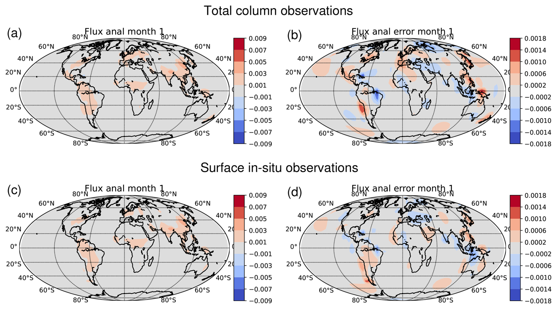
Figure 10 Analyses, ρ^a(0) (left column) and analysis errors (right column) for the quasi-real experiments (units $\mathrm{\mu }\mathrm{g}{\mathrm{m}}^{-\mathrm{2}}{\mathrm{s}}^{-\mathrm{1}}$). The top row is for TCA and the bottom row is for SIS observations.

5.2 Quasi-real-world situation: the effect of model error

The effect of the model error proxy on these assimilation experiments is smaller than in the source/sink location experiments in Sect. 4. Figure 11 shows the effect of using η=0.7 and 1.3 in the DA. Compared to the η values used in Fig. 6, values of η further from unity are required here to see noticeable effects in the analysis; this is probably because of the presence of the meaningful a priori state here. The first point to note is that all experiments are still able to reduce the error from the background despite the presence of model error. Assimilating SIS observations is more robust against model error than for TCA observations, and it is hard to see differences on the colour scale between the bottom rows of Figs. 11 and 10c. The most noticeable exception is for η=0.7 in panel (c) where there is still some error in the sink field over Indonesia. This anomaly is also present for the η=0.7 TCA experiment, panel (a), but exists together with anomalous sinks over Patagonia, New Zealand, north central Russia, north western Canada, and Greenland. Some of these anomalies (e.g. over Patagonia) are not due to persistent background errors, but result from unaccounted for model error in the DA. The Patagonia anomaly changes sign from an anomalous sink for η=0.7 in (a) to a source for η=1.3 in (b).

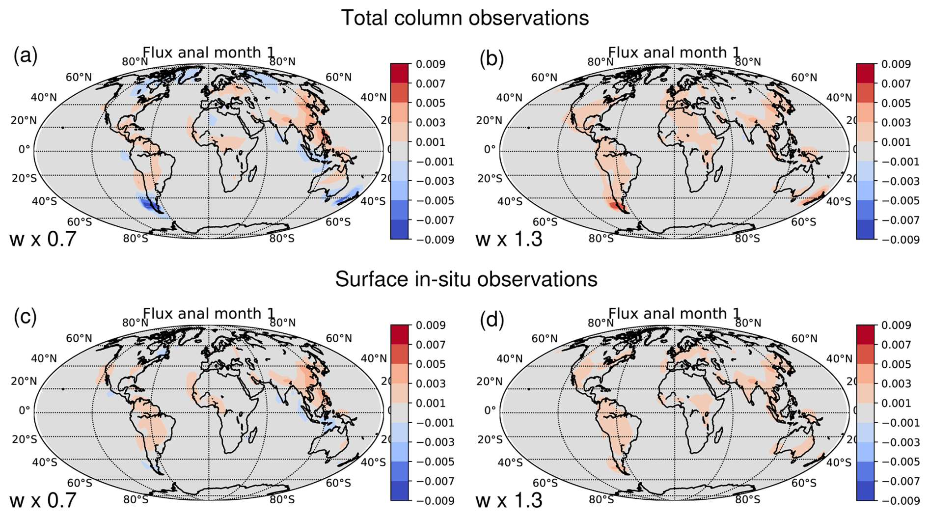
Figure 11 Analyses, ρ^a(0), for the quasi-real experiments found by assimilating either TCA (top row) or SIS observations (bottom row) for the case when a proxy for model error is applied in the assimilation. Model error is simulated by multiplying the vertical wind, w, used in the assimilation by either η=0.7 (panels a and c) or η=1.3 (panels b and d). These plots should be compared to the true field in Fig. 9b (units $\mathrm{\mu }\mathrm{g}{\mathrm{m}}^{-\mathrm{2}}{\mathrm{s}}^{-\mathrm{1}}$).

5.3 Quasi-real-world situation: effect of model error on the on fluxes and analysis errors

A systematic analysis of the way that model error affects the total flux amounts is shown in Fig. 12a (TCA, solid lines; SIS dotted lines, truth dashed line; sources are red and sinks are blue). There is a general tendency of the analysed total fluxes to increase with η for both observation systems (this is straightforward to see for the sources for η>0.9; in the case of the sinks, the absolute value decreases with η for η<1.2, but the actual total sink is minus this value, which increases). This is consistent with the idea that, as the global circulation anomalously speeds up in the forward model used inside the DA (i.e. as η increases), tracer can no longer accumulate near the surface (where the SIS observations are located, and where the highest contribution to the TCA observations is made) and so higher emissions are required to compensate. As found in the flux location experiments (Sect. 4) and here, assimilating the SIS observations systematically gives results closer to the truth than for the TCA observations (this can be seen in panel (a) where the dotted red line (SIS) is closer to the dashed line (truth) than the solid red line (TCA), and the dotted blue line (SIS) is closer to zero (truth) than the solid blue line (TCA)).

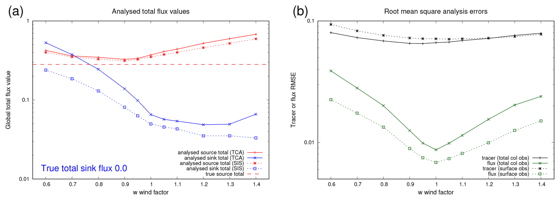
Figure 12 Summary of the effect of model error (via w→ηw) in the quasi-real assimilation experiments. Panel (a) shows the analysed global total source, ${\int }_{{\mathit{\rho }}^{\mathrm{a}}\left(\mathrm{0}\right)>\mathrm{0}}\mathrm{d}A{\mathit{\rho }}^{\mathrm{a}}\left(\mathrm{0}\right)$ (red lines), total sink, $\left|{\int }_{{\mathit{\rho }}^{\mathrm{a}}\left(\mathrm{0}\right)<\mathrm{0}}\mathrm{d}A{\mathit{\rho }}^{\mathrm{a}}\left(\mathrm{0}\right)\right|$ (blue lines) for the TCA (solid) and SIS (dotted) observation experiments. The true total source value is indicated by the dashed horizontal line (the true total sink is zero). Panel (b) shows the root mean square error in the analysed χ^a(0) (black) and ρ^a(0) (green) for the TCA (solid) and SIS (dotted) observation experiments. The units are Tg month⁻¹ for both panels. The units are: global total flux values and errors Tg month⁻¹ and tracer errors Tg.

Interestingly, this result appears to be the reverse of the findings of Basu et al. (2018), who found that TCA observations over land allowed more robust flux analyses than in situ observations. Their explanation concerned unaccounted for convective transport of tracer, which could affect in situ observations more than TCA observations. This is a compelling argument, but it may also be due to any suboptimalities due to incorrectly assigned error characteristics of each observation network, e.g. by incorrectly assigning the representativeness error for in-situ observations. This issue is not studied further here, but could be by introducing scale mis-matches between the in-situ data and the assimilation (e.g. by generating SIS observations from a much higher resolution version of the model, but assimilating them with the lower resolution model).

The effect of model error on the root mean squared analysis errors (RMSEs) is quantified in Fig. 12b. The RMSEs for flux (green lines) reassuringly minimise when η=1 and are smaller for the assimilated SIS observations (dotted line) than for the TCA observations (solid), consistent with previous results. The finding is different for the RMSEs for the initial tracer (black lines). Here the experiment with the smallest RMSE for the TCA observation network is at η=0.95 and for the SIS network is at η=1.05. Further work would be required to decide if these deviations from η=1 are due to the particular background or set of observations.

5.4 Quasi-real-world situation: effect of observation biases on the on fluxes and analysis errors

The final results in this demonstration study shows how the total flux amounts and analysis errors in the quasi-real-world situation vary with observation bias. We find that the presence of bias in this well-observed system does not change the pattern of inferred fluxes from that of the unbiased observation system in the left panels of Fig. 10 (not shown), but does change the flux amounts.

A systematic analysis of the way that observation bias affects the total flux amounts is shown in Fig. 13 for TCA observations (a) and SIS observations (c), where solid lines are the analysed total fluxes (sources are red and sinks are blue), and the red dashed lines represent the true total source (the true total sink is zero in these experiments). The inferred total sources and sinks increase in value as the observation bias increases (the sinks need to be multiplied by −1 to find the actual sink values). This is the same conclusion as for the location experiments in Sect. 4.4. The absolute values of the total sources and sinks are overestimated in all experiments conducted, but as the amounts are found to increase with observation bias, the sources get further from the truth, but the sinks get closer to the truth (the true total sink is zero). This may not be a universal effect as it will probably change with different values of background error standard deviations. The effect on the TCA-observed system is larger than for the SIS-observed system. Recall that the observation biases are varied as a proportion of the random error up to ± just over half of σ° for each observation type, so it is a broadly fair comparison between the two observation networks.

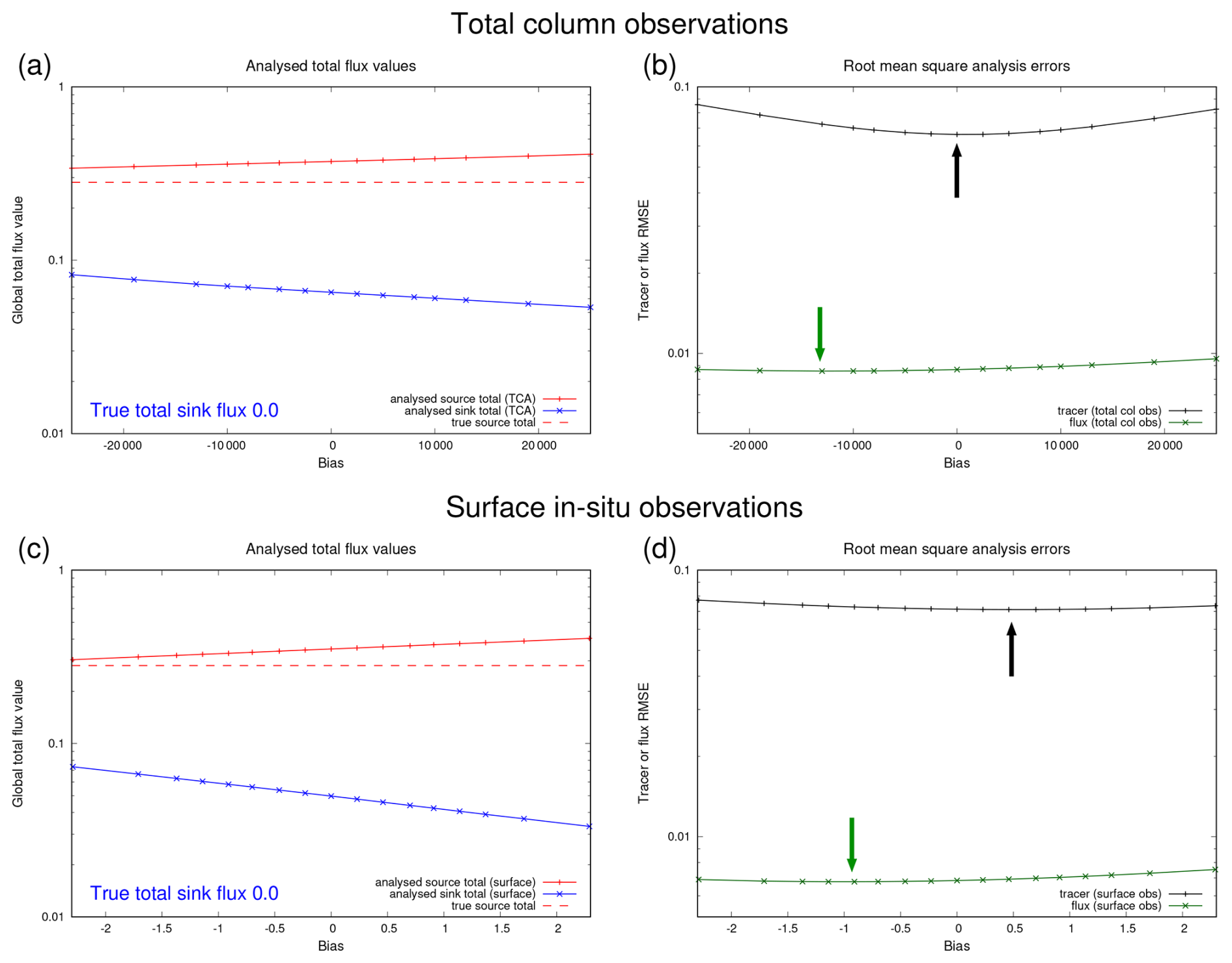
Figure 13 As Fig. 12 but varying observation bias. Panels (a) and (b) are for the TCA observations and (c) and (d) are for the SIS observations. The points with the smallest RMSE values are indicated with arrows.

The RMSE analysis errors in Fig. 13(b) and (d) show minima at the observation bias values indicated with the arrows (these are added as an aid owing to the shallow curves on the logarithmic scale). With the exception of the black line in (b) (for χ^a(0) errors for the TCA observations), the minima in the RMSEs do not align with zero bias. In the case of flux analysis errors, the “optimal” observation biases are negative. This has the effect of reducing the fluxes to values closer to the truth. This is an example of one type of error partially correcting for another (systematic biases compensating for the general overestimation of fluxes in the system), and can make the process of tuning such a DA system a complex task.

6 Summary, conclusions, and further work

6.1 Summary and conclusions

This paper introduces a simplified tool (EnviFlux), to allow investigations into inverse modelling techniques to infer surface fluxes. These techniques have difficulties and shortcomings, mainly because of the indirectness of the observations in order to estimate surface flux information. EnviFlux represents a “back to basics” approach to facilitate a deeper understand of the basic inverse problem without the complexities and expense of other systems, and with no need for high performance computing resources. The tool uses a semi-Lagrangian (SL) transport model, a spectrally modelled B-matrix (which implies homogeneous background error correlations), and supports in situ tracer and flux, and total column amount observations. EnviFlux is a 4D-Var-based inverse model, which estimates the flux field on the same grid as the model, and it does this simultaneously with the initial tracer field. The tool can be used “as is” or can be expanded as required. The software is a suite of programs, mainly written in C++, with some Python visualisation tools. Due to its intentional simplicity, there are some issues that EnviFlux cannot currently explore, such as those specific to satellite measurements (such as cloud and aerosol effects), and with unresolved transport, but it is designed to look at the general problem of extracting information from indirect observations.

EnviFlux is demonstrated in “weakly Bayesian” (where there is missing a priori information, Sect. 4) and Bayesian (where the mean of the a priori PDF is specified, Sect. 5) scenarios. The weakly Bayesian scenario comprises tests to infer the locations and strengths of a source/sink pair at (a priori) unknown locations from a time sequence of observations of the tracer only. The observation network comprises either total column amount (TCA) or surface in situ (SIS) observations, each following the path of a polar orbiting satellite. The former observation network is meant to resemble an actual instrument such as GOSAT, and the latter is a control for comparison. As long as there is no model error (see below) in the data assimilation, the system can successfully determine the locations of the flux features, but with peak values that are too small, and a spatial extent that is too large (the latter property is likely due to the particular lengthscales used to model the B-matrix, and the fundamental smoothing effect of the inversion). A very simple proxy for model error is used by multiplying the vertical wind by a factor η in the inverse system, where η=1 represents a perfect model. This first set of experiments is very sensitive to even small deviations of η from unity (e.g. 0.9 and 1.1), where the ability of the tool to infer even the correct locations of the flux features is compromised. Even though the horizontal wind components are not multiplied by η, the circulation of the tracer can be affected indirectly (the tracer may, e.g. be advected to vertical levels that are affected more or less by jet streams). Observation biases, however (in the ranges tested from −0.57σ° to 0.57σ°, where σ° is the observation error standard deviation in each set of experiments – itself set to be 10 % of the variability of the modelled observations in each case), do not affect the inferred locations, nor the peak values, but do affect the global total source and sink values. These results confirm other work that real-world inverse models need to have minimal imperfections in the forward model.

The Bayesian scenario (also referred to as the quasi-real-world case) uses similar observation networks, but uses methane-like spatial flux distributions as the observed true flux field. In the perfect model run, the choice of observation network has little effect on the ability of the assimilation to infer the correct qualitative structure of the true fluxes, but the in situ observations do offer advantages. Introducing model error gives rise to false sources and sinks. This becomes evident though at higher deviations from η=1 than for the weakly Bayesian experiments, probably owing to the a priori information available to the quasi-real case. Despite this, the assimilation still improves the flux estimates from the a priori. Model error does also quantitatively change the total tracer released and absorbed and for most of the η values tested there is a tendency for the total sources and sinks to increase with η, which is may be due to the assimilation compensating for the faster transport of tracer in space away from the places where the observation operators are most sensitive. Separately, introducing observation bias in the same way as for the weakly Bayesian experiments, has the same effect on the total source and sink. By varying the bias, we find that the lowest RMSE analyses are not found for the experiments when the biases are zero (negative observation biases give the best results). A compelling argument for this is that it is compensating for the total analysed sources, which are too high in these experiments.

6.2 Developments and further research suggestions

It is anticipated that this simplified system as a base can be used and developed further as a low-cost tool to test new ideas in inverse models for research projects and even for student projects. As it stands, EnviFlux is configured for global flux inversion, but could be modified to study regional flux inversion by constructing a suitable limited area grid, transport model, and B-matrix, and introducing lateral boundary conditions, which could themselves become part of the state vector. It is also possible to swap the SL advection scheme with another, e.g. one that is designed to strictly conserve tracer amount, and to include some chemical processes, such as tropospheric hydroxyl sinks, e.g. Nicely et al. (2018), and stratospheric methane oxidation, e.g. Rohs et al. (2006). Where they are found to exist, correlations between observation errors can profoundly affect assimilation, e.g. Waller et al. (2016), Tandeo et al. (2020). By design, the observation networks used in this paper impose no such correlations, but these can be introduced into the observation generation and the R_k matrices. Providing error correlations between observations within the same major time step only is easiest to consider as this would require least development effort in EnviFlux. The way the B-matrix is modelled in this work dictates the horizontal grid to have dimensions $(\mathrm{2}L+\mathrm{1})\times (L+\mathrm{1})$ (see Appendices A–C). Other than that, the choice of B-matrix model in the cost function can be replaced with alternatives, via the square-root (control variable transform) formulation. As long as the resolution is relatively low, an explicit form of the horizontal forecast error covariances could be used, which could e.g. have different lengthscales over the land to ocean to study their effect.

EnviFlux can be simplified further (e.g. by reducing the horizontal and vertical resolution) to allow large ensembles of inversions for tuning purposes, or as mentioned previously, can be made more complex. Adding chemical loss and production would allow closer comparison with real observations (especially for short-lived tracer species and longer transport times), but would add cost, complexity, and potentially non-linearity. The problem would no longer be a pure transport inverse problem and parcel trajectories would be subject to modification of the mixing ratio, potentially dependent on sunlight, cloud cover, temperature, and concentration of other constituents. Should the chemical modification be erroneous, and where the process is observed (directly or downstream), the upstream surface fluxes in the model would likely be spuriously modified to compensate.

In addition to the issues related to the above developments, some ideas and research questions that EnviFlux can contribute to are as follows. How sparse can the observation network be to infer detailed information on the location of new sources and sinks? How can EnviFlux be used to understand which observations contribute to which surface regions (e.g. by estimating the singular vectors of the forward model; example observation footprints are shown in Dadheech and Turner, 2026)? How well can an inverse model determine the timing of transient fluxes (e.g. Lucas et al., 2017)? How precise does the initial condition field need to be to effectively estimate fluxes (the expectation is that a precise initial condition field is needed for flux estimation to be effective Bannister, 2011; Voshtani et al., 2023). How long does an experiment have to run to virtually lose memory of the initial conditions (e.g. Peylin et al., 2005)? How is it possible to tune the background error covariances in real-world cases when they are not well known (e.g. Bannister and Wilson, 2024)? How can model error be accounted for by developing techniques such as inflating the observation error variances (Lin and Gerbig, 2005; Chevallier et al., 2010; Houweling et al., 2010), or by including a model error term throughout the atmosphere? How do different methods of estimating posterior error covariances compare, e.g. Lanczos or quasi-Newton-based, Fisher and Courtier (1995), Meirink et al. (2008b), Niwa and Fujii (2020)? Can the system be used to test the ability of machine learning-based tools to emulate the forward part of the problem (e.g. Dadheech and Turner, 2026)? By adding a simple chemical or land surface processes parametrisation (e.g. Zhang et al., 2017), can the inversion be modified to estimate parameters in those models?

Appendix A: The spectral transforms used to model background error covariances

A1 The forward spectral transform

The forward spectral transform, S_h, is a key part of EnviFlux's covariance model. This transform acts on a vector which is a field increment in the spectral representation (i.e. a function of two integer wavenumbers l and m, see below). The output is a vector in the real space representation (i.e. a function of longitude, λ_i, and co-latitude, φ_j). Co-latitude is zero at the north pole, and so is related to latitude, ϕ, via $\mathit{\phi }=\mathrm{90}-\mathit{\varphi }$. The basis functions of the spectral representation are the spherical harmonic functions, Y_lm(θ,φ):

$$\begin{array}{}\text{(A1)}& {\displaystyle }{\displaystyle }{Y}_{lm}(\mathit{\theta },\mathit{\phi })=\left\{\begin{array}{ll}{\overline{P}}_{lm}\left(\cos \mathit{\phi }\right)\cos \left(m\mathit{\theta }\right)& m\ge \mathrm{0}\\ {\overline{P}}_{l\left|m\right|}\left(\cos \mathit{\phi }\right)\sin \left(\left|m\right|\mathit{\theta }\right)& m<\mathrm{0}.\end{array}\right.\end{array}$$

Here ${\overline{P}}_{lm}$ are the associated Legendre polynomials (ALPs) of degree l and order m, and the bar notation on the ${\overline{P}}_{lm}$ indicates that they are “4π normalised” (other normalisations are possible). Let the representation in spectral space be v_lm, and in real space be x_ij (longitude θ_i, co-latitude φ_j). We have omitted the δ prefixes here for brevity. These are related via the following linear combination:

$$\begin{array}{}\text{(A2)}& {\displaystyle }{\displaystyle }{x}_{ij}=\sum _{l=\mathrm{0}}^L\sum _{m=-l}^l{v}_{lm}{Y}_{lm}({\mathit{\theta }}_i,{\mathit{\phi }}_j),\end{array}$$

where L is the chosen maximum degree. Equation (A2) is the mathematical form of the spectral transform. From the perspective of the transforms, the longitudes are best represented on a regularly spaced grid of 2L+1 points, and the latitudes on a Gaussian grid of L+1 points (Errera and Ménard, 2012; Wieczorek et al., 2018). This is the grid structure assumed here and is used by EnviFlux. The Gaussian grid enables exact quadrature (known as Gauss–Legendre quadrature, see Appendix A2).

In order to translate Eq. (A2) onto a computer, specifically using standard libraries, we do some rewriting. Substituting Eq. (A1) into (A2), separating the l summation into l=0 and l>0 parts, and further separating the m summation into $-l\le m\le -\mathrm{1}$, m=0, and $\mathrm{1}\le m\le l$ parts:

$$\begin{array}{ll}{\displaystyle }& {\displaystyle }{x}_{ij}=v_{\mathrm{00}}{\overline{P}}_{\mathrm{00}}\left(\cos {\mathit{\phi }}_j\right)\\ {\displaystyle }& {\displaystyle }+\sum _{l=\mathrm{1}}^L\left[\sum _{m=-l}^{-\mathrm{1}}{v}_{lm}{\overline{P}}_{l\left|m\right|}\right(\cos {\mathit{\phi }}_j\left)\sin \right(\left|m\right|{\mathit{\theta }}_i)\\ {\displaystyle }& {\displaystyle }+\sum _{m=\mathrm{0}}^l{v}_{lm}{\overline{P}}_{lm}\left(\cos {\mathit{\phi }}_j\right)\cos \left(m{\mathit{\theta }}_i\right)]\\ {\displaystyle }& {\displaystyle }=v_{\mathrm{00}}{\overline{P}}_{\mathrm{00}}\left(\cos {\mathit{\phi }}_j\right)\\ {\displaystyle }& {\displaystyle }+\sum _{l=\mathrm{1}}^L\left[\sum _{m=\mathrm{1}}^l{v}_{l(-m)}{\overline{P}}_{lm}\right(\cos {\mathit{\phi }}_j\left)\sin \right(m{\mathit{\theta }}_i)+v_{l\mathrm{0}}{\overline{P}}_{l\mathrm{0}}(\cos {\mathit{\phi }}_j)\\ {\displaystyle }& {\displaystyle }+\sum _{m=\mathrm{1}}^l{v}_{lm}{\overline{P}}_{lm}\left(\cos {\mathit{\phi }}_j\right)\cos \left(m{\mathit{\theta }}_i\right)].\end{array}$$

The first and third terms can be combined, as can the second and fourth terms:

$$\begin{array}{ll}{\displaystyle }& {\displaystyle }{x}_{ij}=\sum _{l=\mathrm{0}}^L{v}_{l\mathrm{0}}{\overline{P}}_{l\mathrm{0}}\left(\cos {\mathit{\phi }}_j\right)\\ {\displaystyle }& {\displaystyle }+\sum _{l=\mathrm{1}}^L\sum _{m=\mathrm{1}}^l{\overline{P}}_{lm}\left(\cos {\mathit{\phi }}_j\right)\left[v_{l(-m)}\sin \left(m{\mathit{\theta }}_i\right)+v_{lm}\cos \left(m{\mathit{\theta }}_i\right)\right].\end{array}$$

Further, let $v_{lm}=v_{lm}^{\mathrm{R}}$ ($\mathrm{0}\le m\le l$), and $v_{l(-m)}=v_{lm}^{\mathrm{I}}$ ($\mathrm{1}\le m\le l$):

$$\begin{array}{ll}{\displaystyle }& {\displaystyle }{x}_{ij}=\sum _{l=\mathrm{0}}^L{v}_{l\mathrm{0}}^{\mathrm{R}}{\overline{P}}_{l\mathrm{0}}\left(\cos {\mathit{\phi }}_j\right)\\ \text{(A3)}& {\displaystyle }& {\displaystyle }+\sum _{l=\mathrm{1}}^L\sum _{m=\mathrm{1}}^l{\overline{P}}_{lm}\left(\cos {\mathit{\phi }}_j\right)\left[v_{lm}^{\mathrm{R}}\cos \left(m{\mathit{\theta }}_i\right)+v_{lm}^{\mathrm{I}}\sin \left(m{\mathit{\theta }}_i\right)\right].\end{array}$$

This change of labelling means that we do not have to worry about negative wavenumber indices.

The double summation in Eq. (A3) first loops over l, and then loops over m where the upper m limit depends on l. This is summation order 1 in Fig. A1a. In order to compute the above transform with standard software libraries, we first change the summations to the equivalent order 2 in Fig. A1b:

$$\begin{array}{ll}{\displaystyle }& {\displaystyle }{x}_{ij}=\sum _{l=\mathrm{0}}^L{v}_{l\mathrm{0}}^{\mathrm{R}}{\overline{P}}_{l\mathrm{0}}\left(\cos {\mathit{\phi }}_j\right)\\ \text{(A4)}& {\displaystyle }& {\displaystyle }+\sum _{m=\mathrm{1}}^L\sum _{l=m}^L{\overline{P}}_{lm}\left(\cos {\mathit{\phi }}_j\right)\left[v_{lm}^{\mathrm{R}}\cos \left(m{\mathit{\theta }}_i\right)+v_{lm}^{\mathrm{I}}\sin \left(m{\mathit{\theta }}_i\right)\right].\end{array}$$

This can then be split into a Legendre part and a Fourier part. First define the following:

$$\begin{array}{}\text{(A5a)}& {\displaystyle }& {\displaystyle }{\stackrel{\mathrm{̃}}{v}}_m^{\mathrm{R}}\left(\cos {\mathit{\phi }}_j\right)=\sum _{l=m}^L{v}_{lm}^{\mathrm{R}}{\overline{P}}_{lm}\left(\cos {\mathit{\phi }}_j\right)\mathrm{0}\le m\le L\text{(A5b)}& {\displaystyle }& {\displaystyle }{\stackrel{\mathrm{̃}}{v}}_m^{\mathrm{I}}\left(\cos {\mathit{\phi }}_j\right)=\sum _{l=m}^L{v}_{lm}^{\mathrm{I}}{\overline{P}}_{lm}\left(\cos {\mathit{\phi }}_j\right)\mathrm{1}\le m\le L,\end{array}$$

which leaves the rest of the transform as

$$\begin{array}{ll}{\displaystyle }& {\displaystyle }{x}_{ij}={\stackrel{\mathrm{̃}}{v}}_{\mathrm{0}}^{\mathrm{R}}\left(\cos {\mathit{\phi }}_j\right)\\ \text{(A6)}& {\displaystyle }& {\displaystyle }+\sum _{m=\mathrm{1}}^L\left[{\stackrel{\mathrm{̃}}{v}}_m^{\mathrm{R}}\left(\cos {\mathit{\phi }}_j\right)\cos \left(m{\mathit{\theta }}_i\right)+{\stackrel{\mathrm{̃}}{v}}_m^{\mathrm{I}}\left(\cos {\mathit{\phi }}_j\right)\sin \left(m{\mathit{\theta }}_i\right)\right].\end{array}$$

The inputs to this spectral transform are the sets of coefficients in m,l-space $v_{lm}^{\mathrm{R}}$ ($\mathrm{0}\le m\le L$, $m\le l\le L$), and $v_{lm}^{\mathrm{I}}$ ($\mathrm{1}\le m\le L$, $m\le l\le L$). These are transformed to the intermediate sets of coefficients in m,j space, ${\stackrel{\mathrm{̃}}{v}}_m^{\mathrm{R}}\left(\cos {\mathit{\phi }}_j\right)$ and ${\stackrel{\mathrm{̃}}{v}}_m^{\mathrm{I}}\left(\cos {\mathit{\phi }}_j\right)$ using Eqs. (A5) (the “tilde” variables are half in spectral space, half in real space). In the code, these summations are performed explicitly using tables of ALPs pre-calculated from SHTools (Wieczorek et al., 2018). The spectral transform is completed to i,j space (complete real space) using the standard Fourier transform (A6), which is performed exactly by the routine rfft1b in the fftpack library (Swarztrauber et al., 2016). Note that in data assimilation work, the transform from spectral to real space is part of the forward transform (since it is part of the string of operators that go from control space to observation space, HMB^½ in Eq. 5), although readers may be more familiar with the transforms (Eqs. A5 and A6) being referred to an inverse transforms. This is an unfortunate clash of terminology.

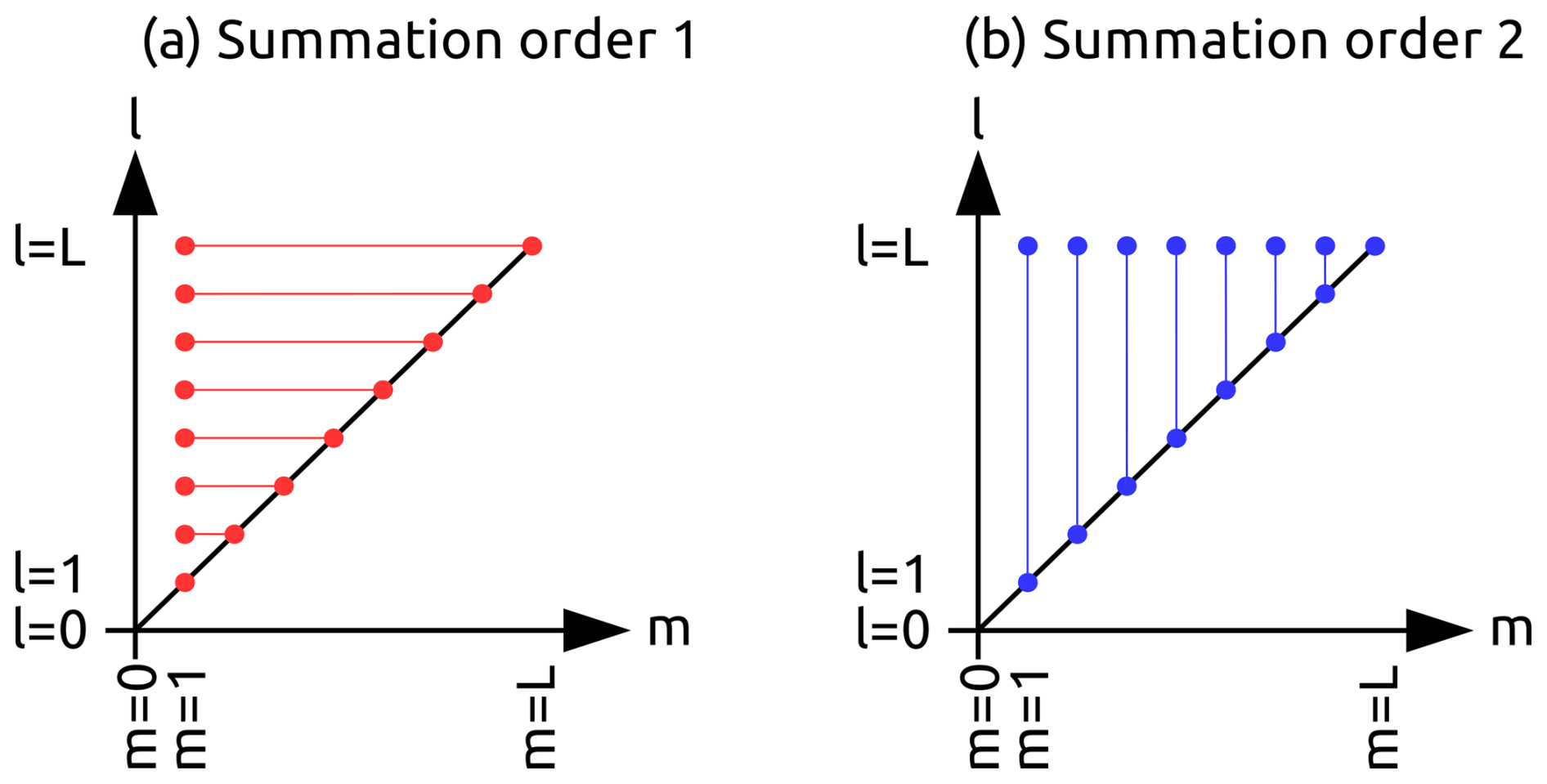
Figure A1 Orders of summations in m and l space as used in transforms (Eqs. A3 and A4). In order 1 (panel a), the sum over l is done first, and in order 2 (panel b), the sum over m is done first. Each order of summation is equivalent to the other as the same points are involved in the double summation.

A2 The inverse spectral transform

The inverse spectral transform, ${\mathbf{S}}_{\mathrm{h}}^{-\mathrm{1}}$, changes the representation of a field increment from real space (a function of longitude, λ_i, and co-latitude, φ_j) to spectral space (a function of the degree, l, and order, m). The inverse of Eqs. (A5) and (A6) is done in reverse order. Firstly, the ${\stackrel{\mathrm{̃}}{v}}_m^{\mathrm{R}}$ and ${\stackrel{\mathrm{̃}}{v}}_m^{\mathrm{I}}$ coefficients are found from standard Fourier transform formulae, which exploit the orthogonality of the sine and cosine functions:

$$\begin{array}{}\text{(A7a)}& {\displaystyle }& {\displaystyle }{\stackrel{\mathrm{̃}}{v}}_{\mathrm{0}}^{\mathrm{R}}\left(\cos {\mathit{\phi }}_j\right)={\displaystyle \frac{\mathrm{1}}{\mathrm{2}L+\mathrm{1}}}\sum _{i=\mathrm{0}}^{\mathrm{2}L}{x}_{ij}\text{(A7b)}& {\displaystyle }& {\displaystyle }{\stackrel{\mathrm{̃}}{v}}_m^{\mathrm{R}}\left(\cos {\mathit{\phi }}_j\right)={\displaystyle \frac{\mathrm{2}}{\mathrm{2}L+\mathrm{1}}}\sum _{i=\mathrm{0}}^{\mathrm{2}L}{x}_{ij}\cos m{\mathit{\theta }}_i\mathrm{1}\le m\le L\text{(A7c)}& {\displaystyle }& {\displaystyle }{\stackrel{\mathrm{̃}}{v}}_m^{\mathrm{I}}\left(\cos {\mathit{\phi }}_j\right)={\displaystyle \frac{\mathrm{2}}{\mathrm{2}L+\mathrm{1}}}\sum _{i=\mathrm{0}}^{\mathrm{2}L}{x}_{ij}\sin m{\mathit{\theta }}_i\mathrm{1}\le m\le L.\end{array}$$

This is the inverse of Eq. (A6) and is performed by the routine rfft1f in the fftpack library. Next the $v_{lm}^{\mathrm{R}}$ and $v_{lm}^{\mathrm{I}}$ (fully spectral) coefficients are found from the formulae (derived below):

$$\begin{array}{ll}{\displaystyle }& {\displaystyle }{v}_{l\mathrm{0}}^{\mathrm{R}}={\displaystyle \frac{\mathrm{1}}{\mathrm{2}}}\sum _{j=\mathrm{0}}^L{\stackrel{\mathrm{̃}}{v}}_{\mathrm{0}}^{\mathrm{R}}\left(\cos {\mathit{\phi }}_j\right){\overline{P}}_{l\mathrm{0}}\left(\cos {\mathit{\phi }}_j\right)\text{GaussWt}\left({\mathit{\phi }}_j\right)\\ \text{(A8a)}& {\displaystyle }& {\displaystyle }\mathrm{0}\le l\le L{\displaystyle }& {\displaystyle }{v}_{lm}^{\mathrm{R}}={\displaystyle \frac{\mathrm{1}}{\mathrm{4}}}\sum _{j=\mathrm{0}}^L{\stackrel{\mathrm{̃}}{v}}_m^{\mathrm{R}}\left(\cos {\mathit{\phi }}_j\right){\overline{P}}_{lm}\left(\cos {\mathit{\phi }}_j\right)\text{GaussWt}\left({\mathit{\phi }}_j\right)\\ \text{(A8b)}& {\displaystyle }& {\displaystyle }\mathrm{1}\le m\le Lm\le l\le L{\displaystyle }& {\displaystyle }{v}_{lm}^{\mathrm{I}}={\displaystyle \frac{\mathrm{1}}{\mathrm{4}}}\sum _{j=\mathrm{0}}^L{\stackrel{\mathrm{̃}}{v}}_m^{\mathrm{I}}\left(\cos {\mathit{\phi }}_j\right){\overline{P}}_{lm}\left(\cos {\mathit{\phi }}_j\right)\text{GaussWt}\left({\mathit{\phi }}_j\right)\\ \text{(A8c)}& {\displaystyle }& {\displaystyle }\mathrm{1}\le m\le Lm\le l\le L,\end{array}$$

where GaussWt(φ_j) are the Gaussian weights (GWs), which are found (together with the ALPs themselves) from the SHtools package. The make up the inverse of Eq. (A5). The GWs allow co-latitude integrals of the following type to be discretised when values f(φ_j) are on Gaussian latitude points φ_j as shown:

$$\begin{array}{}\text{(A9)}& {\displaystyle }{\displaystyle }\underset{\mathit{\phi }=\mathrm{0}}{\overset{\mathit{\pi }}{\int }}f\left(\mathit{\phi }\right)\sin \mathit{\phi }\mathrm{d}\mathit{\phi }=\sum _{j=\mathrm{0}}^{L}f\left({\mathit{\phi }}_j\right)\text{GaussWt}\left({\mathit{\phi }}_j\right).\end{array}$$

Equations (A8) are derived from Eq. (A5) via the following orthogonality property of ALPs:

$$\begin{array}{}\text{(A10)}& {\displaystyle }{\displaystyle }\underset{\mathit{\phi }=\mathrm{0}}{\overset{\mathit{\pi }}{\int }}{\overline{P}}_{lm}\left(\cos \mathit{\phi }\right){\overline{P}}_{l^{\prime }m}\left(\cos \mathit{\phi }\right)\sin \mathit{\phi }\mathrm{d}\mathit{\phi }=\mathrm{2}(\mathrm{2}-{\mathit{\delta }}_{\mathrm{0}m}){\mathit{\delta }}_{l{l}^{\prime }},\end{array}$$

which, using Eq. (A9), becomes

$$\begin{array}{ll}{\displaystyle }& {\displaystyle }\sum _{j=\mathrm{0}}^L{\overline{P}}_{lm}\left(\cos {\mathit{\phi }}_j\right){\overline{P}}_{l^{\prime }m}\left(\cos {\mathit{\phi }}_j\right)\text{GaussWt}\left({\mathit{\phi }}_j\right)=\\ \text{(A11)}& {\displaystyle }& {\displaystyle }\mathrm{2}(\mathrm{2}-{\mathit{\delta }}_{\mathrm{0}m}){\mathit{\delta }}_{l{l}^{\prime }}.\end{array}$$

Multiplying Eq. (A5a) by ${\overline{P}}_{l^{\prime }m}\left(\cos {\mathit{\phi }}_j\right)\text{GaussWt}\left({\mathit{\phi }}_j\right)$, summing over j, and then using Eq. (A11) gives

$$\begin{array}{ll}{\displaystyle }& {\displaystyle }\sum _{j=\mathrm{0}}^L{\stackrel{\mathrm{̃}}{v}}_m^{\mathrm{R}}\left(\cos {\mathit{\phi }}_j\right){\overline{P}}_{l^{\prime }m}\left(\cos {\mathit{\phi }}_j\right)\text{GaussWt}\left({\mathit{\phi }}_j\right)=\\ {\displaystyle }& {\displaystyle }\sum _{l=m}^L{v}_{lm}^{\mathrm{R}}\sum _{j=\mathrm{0}}^L{\overline{P}}_{lm}\left(\cos {\mathit{\phi }}_j\right){\overline{P}}_{l^{\prime }m}\left(\cos {\mathit{\phi }}_j\right)\text{GaussWt}\left({\mathit{\phi }}_j\right)& {\displaystyle }\mathrm{0}\le m\le L\\ {\displaystyle }& {\displaystyle }=\mathrm{2}(\mathrm{2}-{\mathit{\delta }}_{\mathrm{0}m})\sum _{l=m}^L{v}_{lm}^{\mathrm{R}}{\mathit{\delta }}_{l{l}^{\prime }}\\ {\displaystyle }& {\displaystyle }=\mathrm{2}(\mathrm{2}-{\mathit{\delta }}_{\mathrm{0}m})v_{l^{\prime }m}^{\mathrm{R}}\text{for }m\le l^{\prime }\le L.\end{array}$$

When m=0 this gives Eq. (A8a) and when $\mathrm{1}\le m\le L$ this gives Eq. (A8b). Now multiplying Eq. (A5b) by ${\overline{P}}_{l^{\prime }m}\left(\cos {\mathit{\phi }}_j\right)\text{GaussWt}\left({\mathit{\phi }}_j\right)$, summing over j, and then using Eq. (A11) similarly gives

$$\begin{array}{ll}{\displaystyle }& {\displaystyle }\sum _{j=\mathrm{0}}^L{\stackrel{\mathrm{̃}}{v}}_m^{\mathrm{I}}\left(\cos {\mathit{\phi }}_j\right){\overline{P}}_{l^{\prime }m}\left(\cos {\mathit{\phi }}_j\right)\text{GaussWt}\left({\mathit{\phi }}_j\right)=\\ {\displaystyle }& {\displaystyle }\sum _{l=m}^L{v}_{lm}^{\mathrm{I}}\sum _{j=\mathrm{0}}^L{\overline{P}}_{lm}\left(\cos {\mathit{\phi }}_j\right){\overline{P}}_{l^{\prime }m}\left(\cos {\mathit{\phi }}_j\right)\text{GaussWt}\left({\mathit{\phi }}_j\right)\mathrm{1}\le m\le L\\ {\displaystyle }& {\displaystyle }=\mathrm{2}(\mathrm{2}-{\mathit{\delta }}_{\mathrm{0}m})\sum _{l=m}^L{v}_{lm}^{\mathrm{I}}{\mathit{\delta }}_{l{l}^{\prime }}\\ {\displaystyle }& {\displaystyle }=\mathrm{2}(\mathrm{2}-{\mathit{\delta }}_{\mathrm{0}m})v_{l^{\prime }m}^{\mathrm{I}}\text{for }m\le l^{\prime }\le L.\end{array}$$

The m=0 case is of no interest, which leaves only the cases when $\mathrm{1}\le m\le L$, which gives Eq. (A8c).

A3 The adjoint spectral transform

The adjoint of the spectral transform (which is part of ${\mathbf{B}}^{\frac{⊺}{\mathrm{2}}}$) is needed to compute implied covariances (${\mathbf{B}}^{\frac{\mathrm{1}}{\mathrm{2}}}{\mathbf{B}}^{\frac{⊺}{\mathrm{2}}}$) and the gradient of the cost function (Eq. 6). Given that the adjoint operator is mathematically equivalent to the operator that propagates gradients (in the reverse direction to the forward counterparts), we use this equivalence as a means of deriving the adjoint versions of Eqs. (A6) and (A5). Let variables with a hat represent gradients (of some unspecified function) with respect to that variable, namely $\widehat{z}=\partial /\partial z$.

We will start with Eq. (A6), and look at the gradient with respect to each input component (${\stackrel{\mathrm{̃}}{v}}_{\mathrm{0}}^{\mathrm{R}}\left(\cos {\mathit{\phi }}_j\right)$, ${\stackrel{\mathrm{̃}}{v}}_m^{\mathrm{R}}\left(\cos {\mathit{\phi }}_j\right)$, and ${\stackrel{\mathrm{̃}}{v}}_m^{\mathrm{I}}\left(\cos {\mathit{\phi }}_j\right)$), and exploit the chain rule in each case. The first input component of the forward transform (Eq. A6) is ${\stackrel{\mathrm{̃}}{v}}_{\mathrm{0}}^{\mathrm{R}}\left(\cos {\mathit{\phi }}_j\right)$. The gradient with respect to this variable, ${\widehat{\stackrel{\mathrm{̃}}{v}}}_{\mathrm{0}}^{\mathrm{R}}\left(\cos {\mathit{\phi }}_j\right)$, is the output of the adjoint operation:

$$\begin{array}{}\text{(A12)}& {\displaystyle }{\displaystyle }{\widehat{\stackrel{\mathrm{̃}}{\mathit{\chi }}}}_{\mathrm{0}}^{\mathrm{R}}\left(\cos {\mathit{\phi }}_j\right)=\sum _{i=\mathrm{0}}^{\mathrm{2}L}{\displaystyle \frac{\partial x_{ij}}{\partial {\stackrel{\mathrm{̃}}{v}}_{\mathrm{0}}^{\mathrm{R}}\left(\cos {\mathit{\phi }}_j\right)}}{\widehat{x}}_{ij}=\sum _{i=\mathrm{0}}^{\mathrm{2}L}{\widehat{x}}_{ij},\end{array}$$

where the partial derivative is found from Eq. (A6). The next group of input components to Eq. (A6) is ${\stackrel{\mathrm{̃}}{v}}_m^{\mathrm{R}}\left(\cos {\mathit{\phi }}_j\right)$ ($\mathrm{1}\le m\le L$). The gradient with respect to this variable, ${\widehat{\stackrel{\mathrm{̃}}{v}}}_m^{\mathrm{R}}\left(\cos {\mathit{\phi }}_j\right)$, is another output of the adjoint operation and is calculated are a similar way:

$$\begin{array}{ll}{\displaystyle }& {\displaystyle }{\widehat{\stackrel{\mathrm{̃}}{v}}}_m^{\mathrm{R}}\left(\cos {\mathit{\phi }}_j\right)\sum _{i=\mathrm{0}}^{\mathrm{2}L}{\displaystyle \frac{\partial x_{ij}}{\partial {\stackrel{\mathrm{̃}}{v}}_m^{\mathrm{R}}\left(\cos {\mathit{\phi }}_j\right)}}{\widehat{x}}_{ij}=\sum _{i=\mathrm{0}}^{\mathrm{2}L}\cos \left(m{\mathit{\theta }}_i\right){\widehat{x}}_{ij}\\ \text{(A13)}& {\displaystyle }& {\displaystyle }m\le l\le L.\end{array}$$

The final group of input components is ${\stackrel{\mathrm{̃}}{v}}_m^{\mathrm{I}}\left(\cos {\mathit{\phi }}_j\right)$ ($\mathrm{1}\le m\le L$) and are calculated in a similar way:

$$\begin{array}{ll}{\displaystyle }& {\displaystyle }{\widehat{\stackrel{\mathrm{̃}}{v}}}_m^{\mathrm{I}}\left(\cos {\mathit{\phi }}_j\right)\sum _{i=\mathrm{0}}^{\mathrm{2}L}{\displaystyle \frac{\partial x_{ij}}{\partial {\stackrel{\mathrm{̃}}{v}}_m^{\mathrm{I}}\left(\cos {\mathit{\phi }}_j\right)}}{\widehat{x}}_{ij}=\sum _{i=\mathrm{0}}^{\mathrm{2}L}\sin \left(m{\mathit{\theta }}_i\right){\widehat{x}}_{ij}\\ \text{(A14)}& {\displaystyle }& {\displaystyle }m\le l\le L.\end{array}$$

Notice that the adjoint operators (Eqs. A12–A14) are similar to the inverse Fourier formulae (Eqs. A7a–A7c) respectively, but with no prefactors. This means that the rfft1f routine in the fftpack library can be used to perform the adjoint.

The next adjoint step is of Eq. (A5), and we will look at the gradient with respect to each input component ($v_{lm}^{\mathrm{R}}$ and $v_{lm}^{\mathrm{I}}$). The first group of input components of the forward transform (Eq. A5) is $v_{lm}^{\mathrm{R}}$:

$$\begin{array}{ll}{\displaystyle }& {\displaystyle }{\widehat{v}}_{lm}^{\mathrm{R}}=\sum _{j=\mathrm{0}}^L{\displaystyle \frac{\partial {\stackrel{\mathrm{̃}}{v}}_m^{\mathrm{R}}\left(\cos {\mathit{\phi }}_j\right)}{\partial v_{lm}^{\mathrm{R}}}}{\widehat{\stackrel{\mathrm{̃}}{v}}}_m^{\mathrm{R}}\left(\cos {\mathit{\phi }}_j\right)=\\ {\displaystyle }& {\displaystyle }\sum _{j=\mathrm{0}}^L{\overline{P}}_{lm}\left(\cos {\mathit{\phi }}_j\right){\widehat{\stackrel{\mathrm{̃}}{v}}}_m^{\mathrm{R}}\left(\cos {\mathit{\phi }}_j\right)\\ \text{(A15)}& {\displaystyle }& {\displaystyle }\mathrm{0}\le m\le L,m\le l\le L.\end{array}$$

The final group of input components is $v_{lm}^{\mathrm{I}}$:

$$\begin{array}{ll}{\displaystyle }& {\displaystyle }{\widehat{v}}_{lm}^{\mathrm{I}}=\sum _{j=\mathrm{0}}^L{\displaystyle \frac{\partial {\stackrel{\mathrm{̃}}{v}}_m^{\mathrm{I}}\left(\cos {\mathit{\phi }}_j\right)}{\partial v_{lm}^{\mathrm{I}}}}{\widehat{\stackrel{\mathrm{̃}}{v}}}_m^{\mathrm{I}}\left(\cos {\mathit{\phi }}_j\right)=\\ {\displaystyle }& {\displaystyle }\sum _{j=\mathrm{0}}^L{\overline{P}}_{lm}\left(\cos {\mathit{\phi }}_j\right){\widehat{\stackrel{\mathrm{̃}}{v}}}_m^{\mathrm{I}}\left(\cos {\mathit{\phi }}_j\right)\\ \text{(A16)}& {\displaystyle }& {\displaystyle }\mathrm{1}\le m\le L,m\le l\le L.\end{array}$$

Notice that the adjoint operators (Eqs. A15 and A16) are similar to the inverse Legendre formulae (Eqs. A8b and A8c) respectively, but with different scaling (specifically no prefactors and no Gaussian weights).

The above steps are needed to perform the adjoint of the spectral transform in terms of separate Fourier and Legendre steps. It is also possible to write the adjoint of the whole horizontal transform (Eq. A2) in one go:

$$\begin{array}{ll}{\displaystyle }& {\displaystyle }{\widehat{v}}_{lm}=\sum _{j=\mathrm{0}}^L\sum _{i=\mathrm{0}}^{\mathrm{2}L}{Y}_{lm}({\mathit{\theta }}_i,{\mathit{\phi }}_j){\widehat{x}}_{ij}\\ \text{(A17)}& {\displaystyle }& {\displaystyle }\mathrm{0}\le l\le L,-l\le m\le l,\end{array}$$

which is useful for the calibration of the horizontal transform (Appendix C1).

Appendix B: The practical application of the operators in Eq. (8)

B1 Application of the horizontal transform

The initial condition (ic) part of the control vector for use with the upper left part of Eq. (8) is a field that is a function of l, m, and height z, $\mathit{\delta }\mathit{\chi }\left(\mathrm{0}\right)(l,m,z)$. The ${\mathbf{R}}_{\mathrm{h}}{\mathbf{S}}_{\mathrm{h}}{\mathbf{\Lambda }}_{\mathrm{h}\mathit{\chi }}^{\frac{\mathrm{1}}{\mathrm{2}}}$ part of the CVT does the following. Let the lth diagonal element of ${\mathbf{\Lambda }}_{\mathrm{h}\mathit{\chi }}^{\frac{\mathrm{1}}{\mathrm{2}}}$ be ${\mathbf{\Lambda }}_{\mathrm{h}\mathit{\chi }}^{\frac{\mathrm{1}}{\mathrm{2}}}\left(l\right)$. The action of ${\mathbf{\Lambda }}_{\mathrm{h}\mathit{\chi }}^{\frac{\mathrm{1}}{\mathrm{2}}}$ is to multiply $\mathit{\delta }\mathit{\chi }\left(\mathrm{0}\right)(l,m,z)$ by ${\mathbf{\Lambda }}_{\mathrm{h}c}^{\frac{\mathrm{1}}{\mathrm{2}}}\left(l\right)$. The resulting fields then pass through the S_h operator (separately for each z) resulting in a function of $\mathit{\lambda },\mathit{\phi },z$. S_h outputs on a Gaussian grid with the meridional coordinate being co-latitude (see Appendix A1). R_h translates the co-latitudes, φ, to latitudes, ϕ. In general applications the R_h operator may be also used to interpolate from the Gaussian grid to a different grid. This is not necessary in EnviFlux as it uses a Gaussian grid.

The flux part of the control vector for use with the lower right part of Eq. (8) is a field that is a function of l, m, and time t, $\mathit{\rho }(l,m,t)$. The ${\mathbf{R}}_{\mathrm{h}}{\mathbf{S}}_{\mathrm{h}}{\mathbf{\Lambda }}_{\mathrm{h}\mathit{\rho }}^{\frac{\mathrm{1}}{\mathrm{2}}}$ part of the CVT does a similar thing as for the initial conditions, apart from acting on each t separately, and so the result being a function of $\mathit{\lambda },\mathit{\varphi },t$.

B2 Application of the vertical transform

Following on from the horizontal and reconfiguration transforms for the ic fields, the vertical transform, ${\mathbf{F}}_{\mathrm{v}\mathit{\chi }}{\mathbf{\Lambda }}_{\mathrm{v}\mathit{\chi }}^{\frac{\mathrm{1}}{\mathrm{2}}}{\mathbf{F}}_{\mathrm{v}\mathit{\chi }}^{⊺}$, acts on ic fields that are a function of $\mathit{\lambda },\mathit{\varphi },z$. F_vχ and Λ_vχ are each n_z×n_z matrices and Λ_vc is diagonal. ${\mathbf{F}}_{\mathrm{v}\mathit{\chi }}^{⊺}$ projects onto vertical modes (the eigenvectors), ${\mathbf{\Lambda }}_{\mathrm{v}\mathit{\chi }}^{\frac{\mathrm{1}}{\mathrm{2}}}$ scales the projections, and F_vχ projects from the vertical modes back to z. This is done for each horizontal position separately. In EnviFlux, F_vχ and ${\mathbf{\Lambda }}_{\mathrm{v}\mathit{\chi }}^{\frac{\mathrm{1}}{\mathrm{2}}}$ are independent of longitude and latitude. The output of the vertical transform is also a function of $\mathit{\lambda },\mathit{\varphi },z$.

B3 Application of the temporal transform

Following on from the horizontal and reconfiguration transforms for the flux fields, the temporal transform, ${\mathbf{F}}_{\mathrm{t}\mathit{\rho }}{\mathbf{\Lambda }}_{\mathrm{t}\mathit{\rho }}^{\frac{\mathrm{1}}{\mathrm{2}}}{\mathbf{F}}_{\mathrm{t}\mathit{\rho }}^{⊺}$, acts on fields that are a function of $\mathit{\lambda },\mathit{\varphi },t$. F_tρ and Λ_tρ are each $(T+\mathrm{1})\times (T+\mathrm{1})$ matrices, and Λ_tρ is diagonal. ${\mathbf{F}}_{\mathrm{t}\mathit{\rho }}^{⊺}$ projects onto temporal modes (the eigenvectors), ${\mathbf{\Lambda }}_{\mathrm{t}\mathit{\rho }}^{\frac{\mathrm{1}}{\mathrm{2}}}$ scales the projections, and F_tρ projects from the temporal modes back to t. This is done for each horizontal position separately. The ${\mathbf{\Lambda }}_{\mathrm{t}\mathit{\rho }}^{\frac{\mathrm{1}}{\mathrm{2}}}$ is the same for each horizontal position. The output of the temporal transform is also a function of $\mathit{\lambda },\mathit{\varphi },t$.

Appendix C: Determining the transform matrices

Equation (8) is the form of the spectral-based control variable transform. The objects to be determined are the following: F_vχ, Λ_vχ, Λ_hχ, F_tρ, Λ_tρ, and Λ_hρ. The calibration procedures for determining the above objects are described here.

C1 Determining the variance spectra of the horizontal transforms

The horizontal transforms for the ic and the flux fields are each described in the form ${\mathbf{S}}_{\mathrm{h}}{\mathbf{\Lambda }}_{\mathrm{h}}^{\frac{\mathrm{1}}{\mathrm{2}}}$, where S_h is the spectral transform (spherical harmonics to longitude/co-latitude, Sect. A1), ${\mathbf{\Lambda }}_{\mathrm{h}}^{\frac{\mathrm{1}}{\mathrm{2}}}={\mathbf{\Lambda }}_{\mathrm{h}\mathit{\rho }}^{\frac{\mathrm{1}}{\mathrm{2}}}$ for the ic, and ${\mathbf{\Lambda }}_{\mathrm{h}}^{\frac{\mathrm{1}}{\mathrm{2}}}={\mathbf{\Lambda }}_{\mathrm{h}\mathit{\rho }}^{\frac{\mathrm{1}}{\mathrm{2}}}$ for the flux. This section describes how Λ_h can be determined given a prescribed form of the horizontal correlations.

The implied correlation is found by ${\mathbf{S}}_{\mathrm{h}}{\mathbf{\Lambda }}_{\mathrm{h}}^{\frac{\mathrm{1}}{\mathrm{2}}}{\left({\mathbf{S}}_{\mathrm{h}}{\mathbf{\Lambda }}_{\mathrm{h}}^{\frac{\mathrm{1}}{\mathrm{2}}}\right)}^{⊺}={\mathbf{S}}_{\mathrm{h}}{\mathbf{\Lambda }}_{\mathrm{h}}{\mathbf{S}}_{\mathrm{h}}^{⊺}$. Using the spectral transform (Eq. A2) and the adjoint (A17), the result of acting with ${\mathbf{S}}_{\mathrm{h}}{\mathbf{\Lambda }}_{\mathrm{h}}{\mathbf{S}}_{\mathrm{h}}^{\mathrm{T}}$ on a field that is a function of longitude λ_i and co-latitude φ_j (f(λ_i,φ_j)), giving $f^{\prime }\left({\mathit{\lambda }}_{i^{\prime }}{\mathit{\phi }}_{j^{\prime }}\right)$ is

$$\begin{array}{ll}{\displaystyle }& {\displaystyle }{f}^{\prime }\left({\mathit{\lambda }}_{i^{\prime }}{\mathit{\phi }}_{j^{\prime }}\right)=\\ {\displaystyle }& {\displaystyle }\underset{{\mathbf{S}}_{\mathrm{h}}}{\underbrace{\sum _{l=\mathrm{0}}^L\sum _{m=-l}^l{Y}_{lm}({\mathit{\theta }}_{i^{\prime }},{\mathit{\phi }}_{j^{\prime }})}}\underset{{\mathbf{\Lambda }}_{\mathrm{h}}}{\underbrace{{\mathbf{\Lambda }}_{\mathrm{h}}(l,m)}}\underset{{\mathbf{S}}_{\mathrm{h}}^{\mathrm{T}}}{\underbrace{\sum _{j=\mathrm{0}}^L\sum _{i=\mathrm{0}}^{\mathrm{2}L}{Y}_{lm}({\mathit{\theta }}_i,{\mathit{\phi }}_j)}}f({\mathit{\lambda }}_i,{\mathit{\phi }}_j).\end{array}$$

In this paper, Λ_h is function of l only:

$$\begin{array}{ll}{\displaystyle }& {\displaystyle }{f}^{\prime }\left({\mathit{\lambda }}_{i^{\prime }}{\mathit{\phi }}_{j^{\prime }}\right)=\sum _{j=\mathrm{0}}^L\sum _{i=\mathrm{0}}^{\mathrm{2}L}\sum _{l=\mathrm{0}}^L{\mathbf{\Lambda }}_{\mathrm{h}}\left(l\right)\\ \text{(C1)}& {\displaystyle }& {\displaystyle }\times \sum _{m=-l}^l{Y}_{lm}({\mathit{\theta }}_{i^{\prime }},{\mathit{\phi }}_{j^{\prime }})Y_{lm}({\mathit{\theta }}_i,{\mathit{\phi }}_j)f({\mathit{\lambda }}_i,{\mathit{\phi }}_j).\end{array}$$

The addition theorem of spherical harmonics (see e.g. Appendix A3, Eq. (A9) of Errera and Ménard, 2012) is

$$\begin{array}{}\text{(C2)}& {\displaystyle }{\displaystyle }\sum _{m=-l}^l{Y}_{lm}({\mathit{\theta }}_{i^{\prime }},{\mathit{\phi }}_{j^{\prime }})Y_{lm}({\mathit{\theta }}_i,{\mathit{\phi }}_j)=\sqrt{\mathrm{2}l+\mathrm{1}}{\overline{P}}_{l\mathrm{0}}\left(\cos \mathit{\alpha }\right),\end{array}$$

where α is the great circle angular separation between positions $({\mathit{\theta }}_{i^{\prime }},{\mathit{\phi }}_{j^{\prime }})$ and (θ_i,φ_j). Substituting Eq. (C2) into (C1) gives the convolution,

$${\displaystyle }{f}^{\prime }\left({\mathit{\lambda }}_{i^{\prime }}{\mathit{\phi }}_{j^{\prime }}\right)=\sum _{j=\mathrm{0}}^L\sum _{i=\mathrm{0}}^{\mathrm{2}L}\underset{\text{implied correlation matrix element}}{\underbrace{\sum _{l=\mathrm{0}}^L{\mathbf{\Lambda }}_{\mathrm{h}}\left(l\right)\sqrt{\mathrm{2}l+\mathrm{1}}{\overline{P}}_{l\mathrm{0}}\left(\cos \mathit{\alpha }\right)}}f({\mathit{\lambda }}_i,{\mathit{\phi }}_j).$$

The implied correlation between $({\mathit{\theta }}_{i^{\prime }},{\mathit{\phi }}_{j^{\prime }})$ and (θ_i,φ_j) due to this horizontal transformation is the kernel indicated above:

$$\begin{array}{ll}{\displaystyle }& {\displaystyle }{C}_{\mathrm{h}}({\mathit{\lambda }}_{i^{\prime }}{\mathit{\phi }}_{j^{\prime }};{\mathit{\lambda }}_i,{\mathit{\phi }}_j)=C_{\mathrm{h}\mathit{\alpha }}\left(\mathit{\alpha }\right)=\\ \text{(C3)}& {\displaystyle }& {\displaystyle }\sum _{l=\mathrm{0}}^L{\mathbf{\Lambda }}_{\mathrm{h}}\left(l\right)\sqrt{\mathrm{2}l+\mathrm{1}}{\overline{P}}_{l\mathrm{0}}\left(\cos \mathit{\alpha }\right).\end{array}$$

Notice that the right hand side is a function only of the separation between the two positions, α, and not on their individual values nor their relative orientation. These properties are called homogeneity and isotropy respectively. Let C_hα(α) be a prescribed function, e.g. the SOAR function $\left\{\mathrm{1}+\left|d/\mathit{\xi }\right|\right\}\exp \left(-\left|d/\mathit{\xi }\right|\right)$, where $d=\mathit{\alpha }\mathit{\pi }{R}_{\mathrm{E}}/\mathrm{180}$, α is in degrees, R_E is the radius of the Earth, and ξ is the chosen lengthscale of the correlation (specified in the same units as R_E). Multiply each side of Eq. (C3) by ${\overline{P}}_{l^{\prime }\mathrm{0}}\left(\cos \mathit{\alpha }\right)\sin \mathit{\alpha }$, and integrate over $\mathit{\alpha }=\left[\mathrm{0},\mathit{\pi }\right]$:

$$\begin{array}{ll}{\displaystyle }& {\displaystyle }\underset{\mathit{\alpha }=\mathrm{0}}{\overset{\mathit{\pi }}{\int }}{C}_{\mathrm{h}\mathit{\alpha }}\left(\mathit{\alpha }\right){\overline{P}}_{l^{\prime }\mathrm{0}}\left(\cos \mathit{\alpha }\right)\sin \mathit{\alpha }=\sum _{l=\mathrm{0}}^L{\mathbf{\Lambda }}_{\mathrm{h}}\left(l\right)\sqrt{\mathrm{2}l+\mathrm{1}}\\ {\displaystyle }& {\displaystyle }\times \underset{\mathit{\alpha }=\mathrm{0}}{\overset{\mathit{\pi }}{\int }}{\overline{P}}_{l\mathrm{0}}\left(\cos \mathit{\alpha }\right){\overline{P}}_{l^{\prime }\mathrm{0}}\left(\cos \mathit{\alpha }\right)\sin \mathit{\alpha }.\end{array}$$

The orthogonality property (Eq. A10) is then used:

$$\begin{array}{ll}{\displaystyle }& {\displaystyle }\underset{\mathit{\alpha }=\mathrm{0}}{\overset{\mathit{\pi }}{\int }}{C}_{\mathrm{h}\mathit{\alpha }}\left(\mathit{\alpha }\right){\overline{P}}_{l^{\prime }\mathrm{0}}\left(\cos \mathit{\alpha }\right)\sin \mathit{\alpha }=\sum _{l=\mathrm{0}}^L{\mathbf{\Lambda }}_{\mathrm{h}}\left(l\right)\sqrt{\mathrm{2}l+\mathrm{1}}\mathrm{2}{\mathit{\delta }}_{l{l}^{\prime }}\\ {\displaystyle }& {\displaystyle }=\mathrm{2}\sqrt{\mathrm{2}{l}^{\prime }+\mathrm{1}}{\mathbf{\Lambda }}_{\mathrm{h}}\left(l^{\prime }\right).\end{array}$$

The horizontal variance spectrum is then given below in continuous form and then in discrete form using Eq. (A9):

$$\begin{array}{ll}{\displaystyle }& {\displaystyle }{\mathbf{\Lambda }}_{\mathrm{h}}\left(l\right)={\displaystyle \frac{\mathrm{1}}{\mathrm{2}\sqrt{\mathrm{2}l+\mathrm{1}}}}\underset{\mathit{\alpha }=\mathrm{0}}{\overset{\mathit{\pi }}{\int }}{C}_{\mathrm{h}\mathit{\alpha }}\left(\mathit{\alpha }\right){\overline{P}}_{l\mathrm{0}}\left(\cos \mathit{\alpha }\right)\sin \mathit{\alpha }\\ \text{(C4)}& {\displaystyle }& {\displaystyle }={\displaystyle \frac{\mathrm{1}}{\mathrm{2}\sqrt{\mathrm{2}l+\mathrm{1}}}}\sum _{j=\mathrm{0}}^L{C}_{\mathrm{h}\mathit{\alpha }}\left({\mathit{\alpha }}_j\right){\overline{P}}_{l\mathrm{0}}\left(\cos {\mathit{\alpha }}_j\right)\text{GaussWt}\left({\mathit{\alpha }}_j\right).\end{array}$$

It is important to ensure that C_hα(0)=1 (which may not be true due to numerical errors in the above procedure). Once Λ_h(l) is computed with Eq. (C4), C_hα(0)=1 is ensured by multiplying Λ_h(l) by $\mathrm{1}/\left({\sum }_{l=\mathrm{0}}^L{\mathbf{\Lambda }}_{\mathrm{h}}\left(l\right)\sqrt{\mathrm{2}l+\mathrm{1}}{\overline{P}}_{l\mathrm{0}}\left(\mathrm{1}\right)\right)$.

C2 Determining the vertical transform for the initial concentration

The vertical transform is described by the n_z×n_z matrices F_vχ and Λ_vχ (see bullet point 2 of Sect. 3.3.1), where n_z is the number of vertical levels. In principle, there can be a different set of such vertical matrices for each horizontal position. For simplicity, we use just one set of eigenvectors (in F_vχ) and eigenvalues (in Λ_vχ), found from a global vertical correlation matrix (Fig. 3).

The correlation matrices are formed from 10 years (1995–2004) of twice-monthly methane forecasts, first detrended to correct for methane trends (even though there was little methane growth over this period, Rigby et al., 2008).

C3 Determining the temporal transform for the flux

The temporal transform is described by the $(T+\mathrm{1})\times (T+\mathrm{1})$ matrices F_tρ and Λ_tρ (see bullet point 5 of Sect. 3.3.2). First a $(T+\mathrm{1})\times (T+\mathrm{1})$ correlation matrix C^t is formed with matrix elements determined from a SOAR function, ${\mathbf{C}}_{ij}^{\mathrm{t}}=\left\{\mathrm{1}+\left|t_i-t_j\right|/\mathit{\tau }\right\}\exp \left(-\left|t_i-t_j\right|/\mathit{\tau }\right)$, where t_i and t_j are times (in months), and τ is the timescale. F_tρ and Λ_tρ are, respectively, eigenvectors and eigenvalues of C^t.

Appendix D: List of the software tools

The following is a list of the main modules available as part of the EnviFlux software. More details are documented in the user guide (Bannister, 2026b).

• Calibration.f90 Constructs a control variable transform file required for the system to run.

• Master_MakeWinds.cpp Makes suitable wind files from ERA5 winds to the format and resolution of EnviFlux. These drive the transport of the chosen tracer.

• Master_MakeFields.cpp Generates initial conditions and surface flux fields for a run of the forward model.

• Master_Invicat2EnviFlux.cpp Converts data from an INVICAT file to an EnviFlux file.

• Master_ReplaceFirstField.cpp Makes a copy of an EnviFlux file, but replacing the initial conditions from another file.

• Master_GenerateObs.cpp Outputs model observations from a given EnviFlux file.

• Master_MakeBG.cpp makes a background state by perturbing a specified truth with a random perturbation.

• Master_Assimilate.cpp runs 4DVar using a covariance file, a background file, and some observations to produce an analysis.

• Master_CalcError.cpp calculates the difference metrics between two states.

The following is a list of auxiliary modules to test some of the system components.

• Master_TestReadWrite.cpp Tests reading and writing of state and wind data.

• Master_ForwardTraj.cpp Computes the trajectory of a particle advected by the prescribed winds. This is for testing the trajectory code before it is used in the semi-Lagrangian advection scheme.

• Master_AdjointTests_CVT.cpp Tests the adjoints of the control variable transform components.

• Master_AdjointTestsObObs.cpp Tests the adjoint of the observation operators.

• Master_AdjointTests_SemiLagrangian.cpp Tests the adjoint of the semi-Lagrangian advection scheme.

• Master_AdjointTests_SL+ObsOp.cpp Tests the adjoint of the combined semi-Lagrangian advection scheme and the observation operator.

• Master_ImpliedCov.cpp Tests the control variable transform to give some implied covariances.

• Master_GradTest.cpp Tests the gradient produced by the penalty-and-gradient routine in EnviFlux.

The following is an example Python program to process and visualise the output of EnviFlux.

• Plot_PriorPostInc.py Takes information from a control variable transform file, observation files, truth, background, and analysis files to produce histograms, scatter plots, and diagnostic fields.

Appendix E: Computational performance

The EnviFlux configuration used here needs relatively low computational resources as it is designed as a “toy” model with relatively low resolution. Most of the computational time demand is due to the integration of the equations of motion and their adjoint, which are needed for each variational iteration. Table E1 shows estimates of the computational burdens for the configuration used in this paper (Table 1), and projected values for a possible higher resolution system run for a longer time (one year). The numbers show that increasing the resolution can cancel-out the low-cost benefits of EnviFlux.

Table E1 Estimated time and memory demands for EnviFlux for the resolution and integration lengths used in this work ($\sim \mathrm{5.5}\mathit{°}\times \mathrm{5.5}\mathit{°}$ grid boxes and 56 levels for a 100 d assimilation window, as specified in Table 1), and projected values based on the higher resolution of 2.25°×2.25° grid boxes and 56 levels for a year. The times given above are based on a 2012 Linux PC, Intel i5-3450 CPU, 1.8 GHz with 4GB memory. The unboosted values relate to the semi-Lagrangian (SL) model where the departure points are calculated each time via an on-line back-trajectory calculation, while the boosted values relate to the departure points being read from a pre-calculated look-up table.

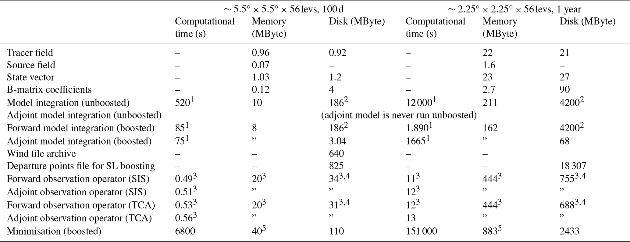
¹ model run with no diffusion; ² disk space assuming tracer output is made every major time step; ³ figures are for 90 000 observations over 100 d or 328 500 observations over one year; ⁴ this is the disk space to store these observations; ⁵ assimilating SIS observations for 25 variational iterations.

Appendix F: The convergence of the cost function

Figure F1 shows how the cost function is reduced for a selection of experiments (see the Fig. key and caption). The 4D-Var is always run with 25 iterations, which are found to be sufficient for near convergence.

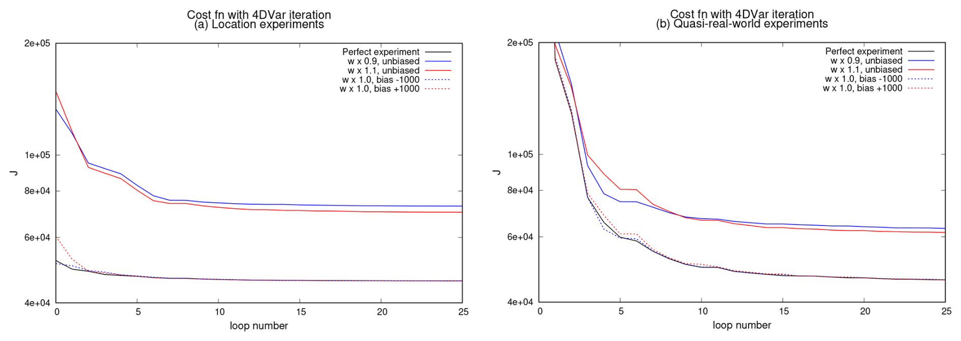
Figure F1 Variation of the cost function, J, Eq. (5), with the 4D-Var loop number. Panel (a) is for a selection of experiments in the weakly Bayesian location regime (Sect. 4) and (b) in the Bayesian quasi-real-world regime (Sect. 5). The black lines are for the perfect experiments (no model error, no observation biases), the coloured continuous lines are for the model error experiments, and the dotted lines are for the observation bias experiments.

Appendix G: The model error scheme

The vertical wind scaling w→ηw, η∼𝒪(1) used in Sects. 4.2, 4.3, 5.2, and 5.3 is meant to be a simple way of adding model error without directly affecting the global (horizontal) circulation of the tracer. Apart from slowing (η<1) or quickening (η>1) vertical transport, scaling only the vertical wind will lead to extra 3D sources and sinks appearing. For interest, this is briefly studied here. The (unmodified) prescribed winds and air density are assumed to be consistent with the standard mass continuity equation:

$$\begin{array}{}\text{(G1)}& {\displaystyle }{\displaystyle \frac{\partial d_z}{\partial t}}+{\mathrm{\nabla }}_{\mathrm{h}}\cdot \left(d_z{\mathit{u}}_{\mathrm{h}}\right)+{\displaystyle \frac{\partial d_{z}w}{\partial z}}=\mathrm{0},\end{array}$$

where d_z is the air density, ∇_h is the horizontal gradient operator, u_h is the horizontal wind vector, $\partial /\partial z$ is the vertical gradient operator, and w is the vertical wind. The scaling, η, affects the tracer (χ) only, making its relevant transport equation as follows:

$$\begin{array}{}\text{(G2)}& {\displaystyle }{\displaystyle \frac{\partial \mathit{\chi }}{\partial t}}+{\mathit{u}}_{\mathrm{h}}\cdot {\mathrm{\nabla }}_{\mathrm{h}}\mathit{\chi }+\mathit{\eta }w{\displaystyle \frac{\partial \mathit{\chi }}{\partial z}}=\mathbf{S}\mathit{\rho }\left(t\right),\end{array}$$

where Sρ(t) is the surface flux term (Sect. 2.1) and where diffusion has been ignored. Multiplying Eq. (G1) by χ, multiplying Eq. (G2) by d_z, adding the resulting equations, as well as adding and subtracting $d_{z}w\partial \mathit{\chi }/\partial z$ gives

$$\begin{array}{ll}{\displaystyle }& {\displaystyle }\underset{\text{combine}}{\underbrace{\mathit{\chi }{\displaystyle \frac{\partial d_z}{\partial t}}+d_z{\displaystyle \frac{\partial \mathit{\chi }}{\partial t}}}}\\ {\displaystyle }& {\displaystyle }+\underset{\text{combine}}{\underbrace{\mathit{\chi }{\mathrm{\nabla }}_{\mathrm{h}}\cdot \left(d_z{\mathit{u}}_{\mathrm{h}}\right)+d_z{\mathit{u}}_{\mathrm{h}}\cdot {\mathrm{\nabla }}_{\mathrm{h}}\mathit{\chi }+\mathit{\chi }{\displaystyle \frac{\partial d_{z}w}{\partial z}}+d_{z}w{\displaystyle \frac{\partial \mathit{\chi }}{\partial z}}}}\\ {\displaystyle }& {\displaystyle }-d_{z}w{\displaystyle \frac{\partial \mathit{\chi }}{\partial z}}+d_z\mathit{\eta }w{\displaystyle \frac{\partial \mathit{\chi }}{\partial z}}=d_z\mathbf{S}\mathit{\rho }\left(t\right).\end{array}$$

By combining the terms indicated, this is equivalent to

$$\begin{array}{}\text{(G3)}& {\displaystyle }{\displaystyle \frac{\partial d_z\mathit{\chi }}{\partial t}}+\mathrm{\nabla }\cdot \left(d_z\mathit{\chi }\mathit{u}\right)=d_z\left[\mathbf{S}\mathit{\rho }\left(t\right)+w(\mathrm{1}-\mathit{\eta }){\displaystyle \frac{\partial \mathit{\chi }}{\partial z}}\right],\end{array}$$

where u is the 3D wind field. Equation (G3) is the continuity equation for χ when the vertical winds are scaled, which yields the “extra” 3D source term $w(\mathrm{1}-\mathit{\eta })\partial \mathit{\chi }/\partial z$, which the inverse model tries to compensate for by producing erroneous surface fluxes.