BuRNN (v1.0): a data-driven fire model

Fires play an important role in the Earth system but remain complex phenomena that are challenging to model numerically. Here, we present the first version of BuRNN, a data-driven model simulating burned area on a global 0.5° × 0.5° grid with a monthly time resolution. We trained Long Short-Term Memory networks to predict satellite-based burned area (GFED5) from a range of climatic, vegetation and socio-economic parameters. We employed a region-based cross-validation strategy to account for the high spatial autocorrelation in our data. BuRNN outperforms the process-based fire models participating in ISIMIP3a on a global scale across a wide range of metrics. Regionally, BuRNN outperforms almost all models across a set of benchmarking metrics in all regions. Through explainable AI we unravel the difference in regional drivers of burned area in our models, showing that the presence/absence of bare ground and C₄ grasses along with the fire weather index have the largest effects on our predictions of burned area. Lastly, we used BuRNN to reconstruct global burned area for 1901–2019 and compare the simulations against independent long-term historical fire observation databases in five countries and the EU. Our approach highlights the potential of machine learning to improve burned area simulations and our understanding of past fire behaviour.

1 Introduction

Fire plays an important role in the Earth system by influencing ecosystem dynamics, biogeochemical cycles and atmospheric composition (Bowman et al., 2020). Fires drive ecosystem dynamics by affecting plant evolution (Simon et al., 2009), vegetation species composition and the physical, chemical and biological properties of soils (McLauchlan et al., 2020). Many of these ecosystem characteristics in turn also shape fire behaviour (Archibald et al., 2018). Emissions from vegetation fires affect the radiative balance of the Earth as the gases (H₂O, CO₂) trap energy through the greenhouse effect, while the aerosols reduce the amount of solar radiation that reaches Earth's surface (Bowman et al., 2009; Ward et al., 2012). Smoke of fires affects a wide range of systems including the radiative balance (Hodzic et al., 2007; Chakrabarty et al., 2023), plant fertilization (Fritze et al., 1994; Bauters et al., 2021), albedo (Beck et al., 2011; Veraverbeke et al., 2012) and air quality (Carvalho et al., 2011; Chen et al., 2017). Fires act as a big natural hazard and can also precondition post-fire hazards such as floods, landslides and large-scale erosion (Zscheischler et al., 2020; Jacobs et al., 2016; Girona-García et al., 2021; Brogan et al., 2017; Shakesby, 2011). Global observations of fire activity are typically provided by satellite products. However, these observations contain substantial uncertainties due to their spatial resolution, cloud cover and temporal resolution affecting their ability to detect small and short-lived fires. Moreover, smoke, rapid regrowth and obscuration by unburned vegetation further complicates satellite-based fire detection. Nonetheless, satellites provide the most reliable estimates of global fire activity to date. Vegetation fires burn approximately 3.5–4.5 million km² of surface area per year (Giglio et al., 2018; Lizundia-Loiola et al., 2020) and emit between 1.8 and 3.0 Pg Cyr⁻¹ (Lizundia-Loiola et al., 2020; van der Werf et al., 2017). More recent estimates from the 5th version of the Global Fire Emissions Database (GFED5) however suggest the amount of surface area burned per year to be around 6.5–9.5 million km² (Chen et al., 2023b) with an emission of 2.9–3.7 Pg Cyr⁻¹ (Chen et al., 2023b), comparable to around 20 %–30 % of the annual emissions from anthropogenic greenhouse gases (Friedlingstein et al., 2025). Fires thus play an active role in our Earth system. Yet, despite their key role, it is not fully understood and quantified how socio-economical development and climate change have affected fire occurrence in the past, and how these will affect future fire dynamics. Moreover, satellite observations suffer uncertainties due to (i) cloud cover, (ii) limited spatial resolution, which affects the detection of small fires, (iii) rapid regrowth and (iv) obscuration by unburned vegetation (Chen et al., 2023b). All of these uncertainties are propagated further into modelling efforts.

To understand how climate change and socio-econmic conditions affect vegetation fires, researchers typically model fire activity with fire-coupled Dynamic Global Vegetation Models (DGVMs; e.g., Burton et al., 2024; Park et al., 2024). These process-based fire models simulate vegetation fires as a function of vegetation characteristics, weather, socio-economic conditions, lightning and land use (Hantson et al., 2016). Vegetation dynamics are typically supplied by the DGVM, while the other factors are provided as inputs derived from climate and integrated assessment models (Frieler et al., 2024). From these drivers, most fire models simulate ignitions (natural + anthropogenic), fuel (dry vegetation), fire spread and fire suppression, which are then transformed to fire characteristics such as burned area, fire intensity and fire emissions (Rabin et al., 2017; Li et al., 2019; Hantson et al., 2020). However, this extensive processing chain requires fine-tuning many parameterizations and formulae, each of which has the potential to alter the outcome substantially. As a result, current state-of-the-art process-based fire models are not always able to reproduce observed fire events (Burton et al., 2024; Park et al., 2024), and their projections contain substantial spread (Teckentrup et al., 2019; Lange et al., 2020; Thiery et al., 2021; Grant et al., 2025). Moreover, (sub)national fire databases are often incomplete and inconsistent (Bowman, 2018; Gincheva et al., 2024)

Machine learning algorithms have the advantage of being able to fit (non-linear) functions to data rather than prescribing them manually. In complex tasks, such as fire modelling, where the real world relations and interactions are hard or near-impossible to pin down mathematically, machine learning can provide a valuable solution (Qi and Majda, 2020; Bracco et al., 2025). At the same time, machine learning often lacks interpretability (Rudin, 2019; Yang et al., 2024; Bracco et al., 2025), which can be a disadvantage compared to process-based models when process understanding or fine-grained control is the primary objective. Thus, machine learning can serve as a complementary rather than a substitutive approach to process-based fire modelling.

Here we present a data-driven fire model “Burned area modelling through Recurrent Neural Networks (BuRNN)”. BuRNN combines traditional fire model inputs and intermediary DGVM outputs such as Gross Primary Productivity (GPP) with machine learning to predict burned area. We first describe the architecture and training process of the model. Then, we evaluate the skill of BuRNN against satellite data, using state-of-the-art process-based wildfire models as benchmark. Next, we attempt to understand the inner workings of BuRNN through eXplainable AI (XAI) methods. Finally, we apply BuRNN to generate a monthly gridded burned area reconstruction from 1901 to 2019 at 0.5° × 0.5° spatial resolution and evaluate this new dataset against regional wildfire records.

2 Materials & Methods

2.1 Data

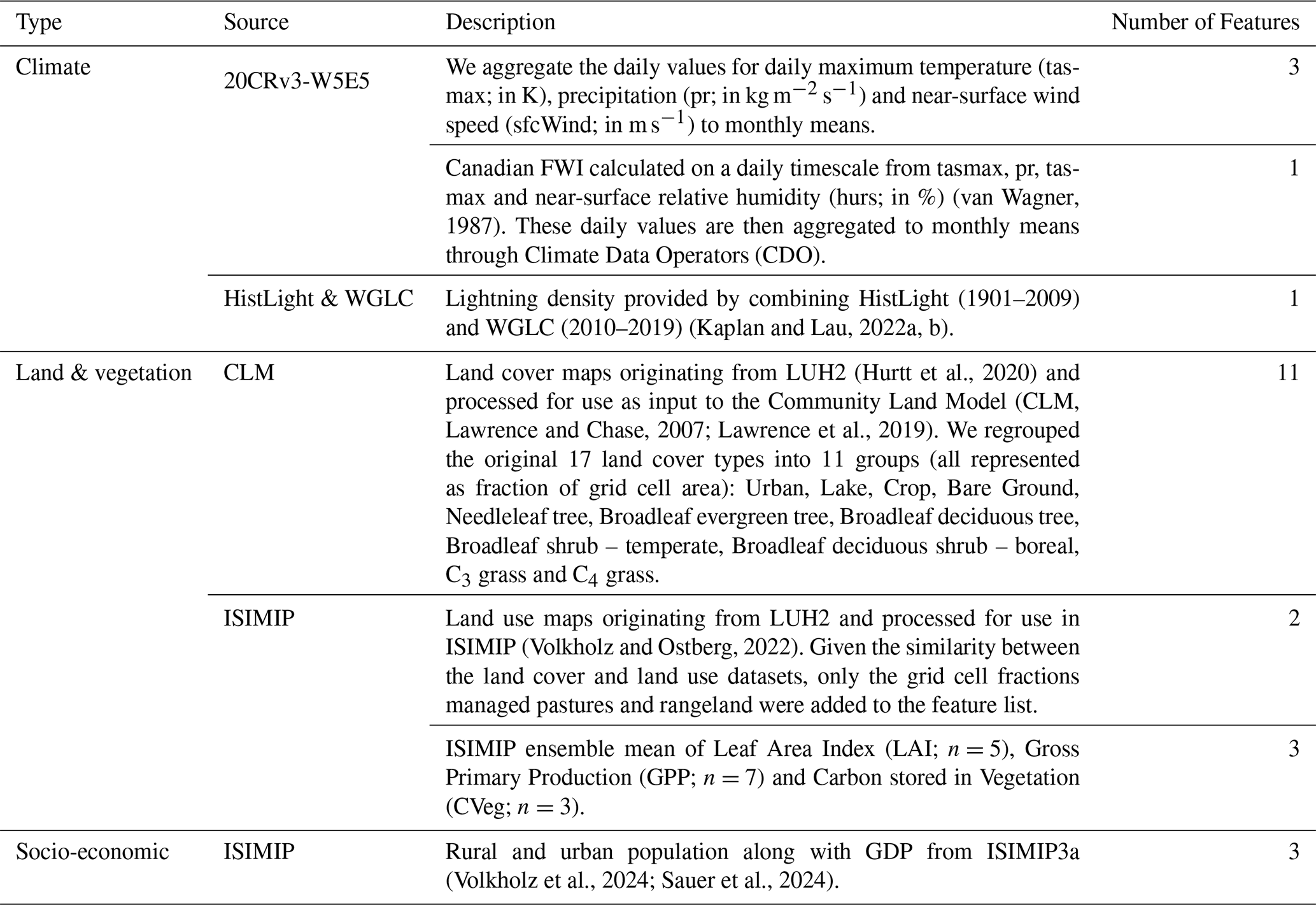
To train BuRNN, we make use of five different data sources. BuRNN is trained on a monthly timescale and receives 24 features as input, each providing information on (i) climate, (ii) land or vegetation properties or (iii) socio-economic conditions (Table 1). Climate-related variables are: (i) monthly mean of the daily maximum temperature, mean monthly precipitation and mean monthly wind speed from the daily NOAA-CIRES-DOE 20th Century Reanalysis version 3 homogenized to W5E5 (20CRv3-W5E5) product (Compo et al., 2011; Slivinski et al., 2021; Lange, 2019; Lange et al., 2021), (ii) monthly mean Fire Weather Index (FWI) calculated from 20CRv3-W5E5 and (iii) lightning density. The land and vegetation characteristics are (i) land cover from the Community Land Model (CLM), which are generated based on Land Use Harmonization phase 2 (LUH2; Hurtt et al., 2020), (ii) land use provided by the Inter-Sectoral Impact Model Intercomparison Project (ISIMIP) also based on LUH2 and (iii) intermediate DGVM outputs (ensemble mean) from the ISIMIP biome sector for GPP (n=7), Carbon mass in Vegetation (CVeg; n=3) and Leaf Area Index (LAI; n=5) (Table A1). Lastly, socio-economic conditions are provided by ISIMIP in terms of population densities and Gross Domestic Product (GDP; Table 1). The LUH2 derived data from ISIMIP and CLM was linearly interpolated from a yearly to monthly timescale. Moreover, we removed and grouped a number of related land use/land cover classes in order to bring the total number of features down. We chose these input variables as all are available on a monthly timescale from 1901 onwards at a 0.5° × 0.5° spatial resolution (or higher) and represent many drivers, or proxies thereof, of fire behaviour. To train BuRNN, we use GFED5 as target data (Chen et al., 2023b), we remapped the original 0.25° × 0.25° grid to 0.5° ×  0.5° using area-weighted regridding from the Python Package Iris – SciTools. GFED5 derives burned area estimates for 2001–2020 from the Moderate Resolution Imaging Spectroradiometer (MODIS) MCD64A1 product (Giglio et al., 2018), applying region-, land cover-, and tree cover-specific corrections for commission and omission errors based on spatiotemporally aligned Landsat and Sentinel-2 burned area observations. Burned area in croplands, peatlands, and deforestation regions is separately estimated using MODIS active fire detections (Giglio et al., 2016). To extend the record back to 1997, active fire data from the Along-Track Scanning Radiometer (ATSR) and the Visible and Infrared Scanner (VIRS) were used, which carry higher uncertainties (Chen et al., 2023b). Although GFED5 almost doubles the observed burned area compared to other satellite products, we consider it most suitable for ground truth as it matches high-resolution burned area observations for Africa (Chuvieco et al., 2022). Moreover, literature suggests that “traditional” burned area products, such as FireCCI51 severely underestimate actual burned area (Zhu et al., 2017; Franquesa et al., 2022; Khairoun et al., 2024), supporting our choice for GFED5 as target dataset.

(van Wagner, 1987)(Kaplan and Lau, 2022a, b)(Hurtt et al., 2020)(CLM, Lawrence and Chase, 2007; Lawrence et al., 2019)(Volkholz and Ostberg, 2022)(Volkholz et al., 2024; Sauer et al., 2024)

Table 1 List of the 24 features provided to BuRNN along with their origin.

2.2 Model Description

We aim to design a machine learning model that is able to learn the lagged and cumulative effects of climate variability, land use and socio-economic conditions on fire dynamics. Unlike traditional machine learning algorithms, which often treat each observation independently, Long Short-Term Memory networks (LSTMs) are capable to capture non-linear temporal dependencies in sequential data (Hochreiter and Schmidhuber, 1997), making them ideal for our use case. Although LSTMs were originally designed for natural language processing (Gers et al., 2000), LSTMs have also successfully been applied in a number of climate related applications such as modelling vegetation dynamics (Reddy and Prasad, 2018), predicting river streamflow (Hunt et al., 2022), weather forecasting (Karevan and Suykens, 2020) and even detection of forest fires (Cao et al., 2019). Therefore, we chose the LSTM as main component of BuRNN. The LSTM maintains its own hidden states acting as memory, which is updated dynamically in interaction with the input features. The hidden state at each time step is mapped to three outputs using a dense neural layer. The first of the outputs is be used as a binary classifier, determining whether it burns or not. The second and third represent parameters (mean and variance) of the modelled burned area distribution. Predicted burned area is constructed via Eq. (1), assuming a normal distribution. Despite the simple model architecture, a couple of hyperparameters have to be chosen. To automate the search for optimal hyperparameters, we used the Optuna framework (Akiba et al., 2019). We used the Tree-structured Parzen Estimator sampler inside the framework to find appropriate values for the learning rate, number of LSTM layers, hidden size of the LSTM layer(s), activation functions, number of dense neural layers, size of the dense neural layers and dropout fraction (Bergstra et al., 2011). Currently, BuRNN is a single layered LSTM with a hidden size of 64 connected to a dense neural layer (see also Fig. 1).

$$\begin{array}{}\text{(1)}& {\displaystyle }\widehat{y}=\mathbf{1}\left\{\widehat{p}>\mathrm{0.5}\right\}\cdot (\mathit{\mu }+\frac{\mathrm{1}}{\mathrm{2}}{\mathit{\sigma }}^{\mathrm{2}})\end{array}$$

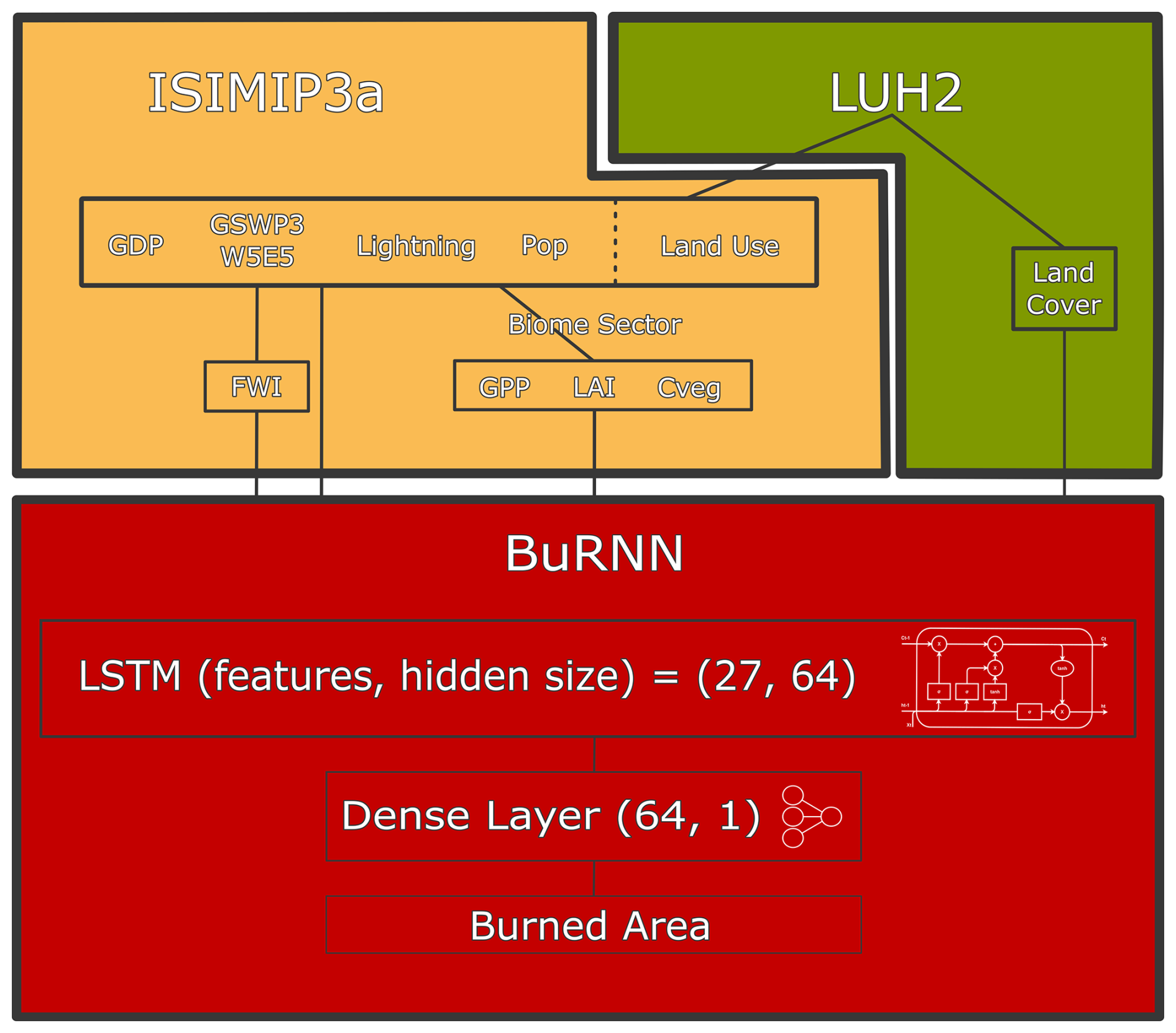
Figure 1 Structure of BuRNN. The top row denotes the origin of all the features supplied to our model, split into the main sources. The red rectangle reflects the architecture of BuRNN.

Given the nature of our data, our input variables (and targets) contain a high degree of spatial autocorrelation. Applying a traditional random train-test split or random train-test folds would likely lead to an overestimation of performance and poor predictive power (Diniz-Filho et al., 2008; Le Rest et al., 2014; Meyer et al., 2019). Therefore, we trained our LSTM networks according to a region-based cross-validation. We split our data according to the 43 Intergovernmental Panel on Climate Change (IPCC) land regions (we removed the two Antarctic regions and Greenland) and manually grouped these regions into 11 folds (Fig. A1), whereby we made sure that the 3–4 regions in each fold represent different continents and biomes (Iturbide et al., 2020). For each fold, we use two different folds as validation set and the remaining 8 folds as training set. We repeat this five times for each fold, each time with two different folds as validation set. For example, when fold 1 is chosen as test fold, we first select folds 2 and 3 as validation set and folds 4–11 as training set. Then we choose folds 4 and 5 as validation set and folds 2–3 and 6–11 as training set, etc. This results in a total of 55 (11 times 5) models. Then, when we make predictions with our model for an IPCC region, it is the mean estimate of five LSTMs which have never seen data for that IPCC region before. The validation folds are used to monitor model convergence and overfitting by using the early stopping algorithm; As soon as model performance on these validation folds started to decrease after a given set of training iterations, training was stopped and the best model was restored. This model was then used to make predictions on the independent test set.

Before training, we combine the data from all different sources, convert the time dimension to have identical units and split them into the 11 pre-defined folds. We normalize the training data and use the mean and standard deviation of the training set to normalize the validation folds (and the test fold during prediction). Each time we change the training folds, we undo the normalization operation, and redo it based on the mean and standard deviation of the new training set. Additionally, we log-transform the target variable (GFED5 percentage burned area) as the original data is strongly right-skewed We do this by applying the natural logarithm of one plus the target (log1p). After this, we normalise the targets by subtracting the mean and dividing by the standard deviation. Pre-processing of our data happens through a combination of Xarray and NumPy. We use PyTorch and PyTorch Lightning to build our model architecture and to handle training and validation (Paszke et al., 2019; Falcon and The PyTorch Lightning team, 2019). In the training phase the LSTM layer is followed by batch normalization. During training, we provide the samples in batches of 32, an error is calculated based on the cumulative error of the predictions for these 32 samples (see further) after which the model is updated/improved. Batch normalization normalizes the features of each batch (based on the batch's mean and standard deviation) and results in faster and more stable training (Santurkar et al., 2018). This layer is followed by a dropout layer for which the optimal dropout fraction was found to be 0.2. This randomly ignores, on average, 20 % of the connections between the LSTM and dense layer, which has been proposed to improve generalisation and reduce overfitting (Srivastava et al., 2014). During training we ignore the first 36 predictions (3 years) to allow the LSTM's memory state to spin up and then evaluate the predictions of the following 3 years using a custom loss function. In each epoch, we pass each gridcell in the training set once and randomly select a 6 year time slice. The spinup period of 3 years was chosen based on fire-process understanding and the prediction length of 3 years was chosen in function of model convergence speed. The loss function expects three outputs from the model, the first is used as a binary classifier (will it burn or not) and is scored through binary cross entropy (Eq. 2), the second represents the mean (log-transformed and normalised) burned area and the third is the (log-transformed and normalised) variance. This mean and variance are used in a Gaussian negative log likelihood loss (Eq. 3). Then, the Gaussian negative log likelihood loss is multiplied by 1000 so it reaches a similar magnitude as the binary cross entropy loss, after which both loss terms are added up. After training, the normalisation and log-transform can be inverted to obtain predictions in fraction of burned area per cell again.

$$\begin{array}{}\text{(2)}& {\mathcal{L}}_{\text{BCE}}(y,\widehat{p})=-\left[y\log \left(\widehat{p}\right)+(\mathrm{1}-y)\log (\mathrm{1}-\widehat{p})\right].\end{array}$$

Here, $y\in \mathit{\{}\mathrm{0},\mathrm{1}\mathit{\}}$ is the binary target (fire occurrence) and $\widehat{p}\in (\mathrm{0},\mathrm{1})$ is the predicted probability of fire occurrence.

$$\begin{array}{}\text{(3)}& {\mathcal{L}}_{\text{NLL}}(y,\mathit{\mu },{\mathit{\sigma }}^{\mathrm{2}})={\displaystyle \frac{\mathrm{1}}{\mathrm{2}}}\left[\log \left({\mathit{\sigma }}^{\mathrm{2}}\right)+{\displaystyle \frac{(y-\mathit{\mu }{)}^{\mathrm{2}}}{{\mathit{\sigma }}^{\mathrm{2}}}}\right].\end{array}$$

Here, y is the observed value, μ is the predicted mean, and σ² is the predicted variance of a Gaussian distribution.

2.3 Model Evaluation

We evaluate our predictions for 2003–2019, the common period between the full availability of Terra/Aqua in MODIS and the ISIMIP fire sector simulations (forced with the GSWP3-W5E5 reanalysis). We evaluate our 3D (time, latitude, longitude) data cubes for several metrics in different dimensions (spatial, temporal and spatio-temporal). By calculating the Root Mean Squared Error (RMSE) between the modelled and observed 3D cubes, we obtain an error expressed in % burned area. Similarly, by calculating the Pearson correlation we obtain a metric that informs on spatial and temporal patterns, ignoring the mean and scale bias the process-based models and BuRNN have (Hantson et al., 2020; Burton et al., 2024). The spatial pattern is evaluated by computing the mean over time, resulting in a 2D data cube (latitude, longitude), and we calculate both spatial RMSE and correlation. Similarly, by taking the sum over the spatial domain (latitude and longitude), we arrive at a monthly and yearly time series of global burned area. We calculate yearly correlation, which assesses the interannual variability, and monthly correlation, which represents seasonality.

2.4 Driver Analysis

To better understand the inner workings of BuRNN, which is in se a black box model, we employ an explainable AI method. Integrated Gradients (IG) is an attribution method for differentiable models, like LSTMs, that quantifies the contribution of each input feature to a specific prediction. IG compares the prediction at an input x to the prediction with a reference baseline input x₀ and integrates the model’s gradients along a straight-line path between them (Sundararajan et al., 2017). Here, we applied the global mean for each feature as baseline. Thus, the IG results need to be interpreted as “How strong does each feature affect burned area in this region compared to the global mean of this feature”. A caveat of this approach is that when a feature in a region tends to be close to the global mean, then attribution for that feature will be low as the integration between sample and baseline will be performed over a short path. Moreover, our approach does not inform on the direction of influence as the direction can vary based on the timing of the feature. For example, precipitation a year before a fire can actually increase burned area by stimulating vegetation growth and increasing future fuel loads, but precipitation right before a fire typically negatively affects burned area. As to not average these two effects out, we take the absolute value of each attribution and thus only look at how important each feature is, not at the actual effect (positive or negative) of each feature. Lastly, highly correlated features will have their attributed importance spread across each other and hence be lower than if only a single of these features was provided. For each of the 55 LSTMs, we pass it the test data of 2002–2008 and attribute the predictions of 2005–2008 (using 2002–2004 as spinup period; see Sect. 2.2) and store this per GFED region. The total number of attributions is the multiplication of the number of models per gridcell (n=5) by the number of land gridcells in the dataset (n=65 797) by each predicted timestep (n=48, since we don't attribute the 3 years spinup i.e., 2002–2004) by the number of features (n=24) and by each considered timestep in the attribution. For the latter, we consider the previous 3 years and the features of the predicted timestep itself (n=37). Resulting in a total of 14 billion attributions, or around 580 million attributions per feature. We take the absolute value of these attributions and average this per region per feature. We note here upfront that IG does not provide causal insights into the real-world processes underlying the data. Instead, IG offers a post hoc explanation of the model’s internal logic by attributing contributions to input features in a way that reflects the model’s learned associations. When applied to structured or interdependent data, IG values can be difficult to interpret because feature dependencies may obscure how importance is distributed, and the method may not capture the full complexity of how the model uses such inputs. Nevertheless, IG can still provide a useful high-level view of the patterns and dependencies the model has learned. Thus, our analysis aims to characterize the statistical associations encoded by the model rather than to infer mechanistic relationships in the underlying system.

2.5 Burned Area Reconstruction

After training, we use the models to simulate burned area for the period 1901–2019. During training we employed a 3 year spinup period (see Sect. 2.2). Therefore, we add 1901–1903 in front of the dataset so this can be used as spinup. We analyse this full reconstruction per region and also compare it against a 1997–2019 run to verify the stability of the model.

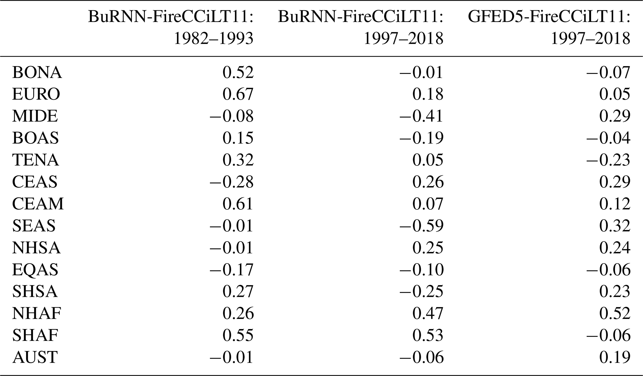
Moreover, we compare the reconstruction to the FireCCiLT11 product, which is based on the Advanced Very-High-Resolution Radiometer (AVHRR; Otón et al., 2021). FireCCiLT11 is available from 1982–2018, with the exception of 1994. We calculate the regional 1982–1993 correlations for annual burned area between BuRNN and FireCCiLT11 and compare those to the 1997–2018 correlations between BuRNN and FireCCiLT11 and between GFED5 and FireCCiLT11. Ideally, the latter values are high, indicating both observational products are in agreement. If this is the case, then a good reconstruction (1982–1993) should have a similar correlation (to FireCCiLT11) for both periods.

Additionally, we compare the reconstruction to regional datasets where available (see Sect. 3.3). For Canada, we assess the National Burned Area Composite (NBAC) and National Fire Database (NFDB) datasets. NBAC is fire polygon database from Landsat (30 m) starting from 1972 and contains data on ∼ 35 000 fires (Canadian Forest Service, 2024). NFDB combines data from various Canadian agencies and contains data for over 700 000 fires between 1959 and 2022 (Hanes et al., 2019). For the Unites States, we compare our reconstruction to the Monitoring Trends in Burn Severity (MTBS) dataset and the Fire Occurrence Database (FOD). MTBS estimates burned area from Landsat and provides data on fires >2 km² since 1984 (Picotte et al., 2020). FOD encompasses fire records from several US agencies for 1992 to 2020 and excludes prescribed burning (Short, 2022). For Brazil we use data from the MapBiomas project, which produces gridded burned area over Brazil from 1985 to 2023 based on Landsat (Souza et al., 2020). For Chile, the database is managed by the Chilean Forest Service (CONAF) and is also based on Landsat, it contains information on over 200 000 fires from 1985 to 2021. We obtained the Chilean data from Gincheva et al. (2024). The European Forest Fire Information System (EFFIS) provides us with country-level data on non-agricultural fires for 21 countries in the EU (excluding Austria, Belgium, Denmark, Ireland, Luxembourg and Malta). The data comes from the individual EU countries and is available for different time periods for each country, the earliest is 1980 for Portugal. Lastly, we also asses fires over Australia, making use of data from over 75 % of the Australian surface area. Data was provided by different state and territory agencies and was combined by Gincheva et al. (2024) and is available from 1950 to 2021. All these datasets come with a number of caveats, especially in the earlier periods. They are (i) often incomplete, (ii) use different protocols between products, but also for different time periods within a dataset and (iii) they report different things (some exclude agricultural and/or managed fires, others exclude small fires) (Gincheva et al., 2024). Nonetheless, they are the best independent reference data we have available.

3 Results

3.1 Model Evaluation

Our global-scale evaluation results highlight that BuRNN outperforms all process-based fire models on each of the skill metrics we consider (Table 2) with respect to GFED5 and in all but one metric with respect to FireCCI51 (Table A7). Moreover, for spatial RMSE, spatial correlation and monthly correlation its performance falls in the inter-observational uncertainty. This implies that BuRNN's performance for these metrics is indiscernible from observational products and that further improvement is meaningless until inter-observational uncertainty is decreased. BuRNN has a RMSE of 1.59, while the process-based fire models fall between 1.92 and 3.00 and inter-observational uncertainty is 1.18. Similarly, the correlation factor is 0.70 between 0.01 and 0.51 for the FireMIP models and 0.85 between GFED5 and FireCCI51. The spatial RMSE of BuRNN is 0.49, the process-based models fall between 0.82 and 1.32 and the inter-observational spatial RMSE is 0.49. The spatial correlation is 0.88 for BuRNN, between −0.01 and 0.67 for the FireMIP models and 0.90 for GFED5 and FireCCI51. Monthly correlation, representing seasonality, is 0.86 for BuRNN, between −0.12 and 0.73 for the FireMIP models and 0.87 for FireCCI51 and GFED5. BuRNN's yearly correlation, representing interannual variability, is 0.87, while it is between −0.37 and 0.76 for the process-based models (Table 2) and 0.94. Three example maps of burned area prediction by BuRNN are shown alongside those of GFED5 and the two best-performing process-based models in Figs. A4, A5 and A6. Hence BuRNN scores better than any other fire model for each considered performance metric (total of 54 model-metric combinations). These evaluation results thus overall indicate that at the global scale, BuRNN largely outperforms state-of-the-art global wildfire models. Figure 4 depicts the mean monthly burned area from GFED5 (upper left), BuRNN (upper right) and the nine FireMIP models. In general, the spatial pattern of BuRNN matches closely the pattern of GFED5. This is made further clear in Fig. 5, which shows the difference in mean monthly burned area between BuRNN and GFED5 (upper right) and between the FireMIP models and GFED5. The density plot in the upper left depicts the distribution of the error over all land pixels for BuRNN and the FireMIP models, where the difference between GFED5 and each of the models is considered the error. The distribution of BuRNN falls more closely around zero than any of the FireMIP models, indicating again better spatial performance.

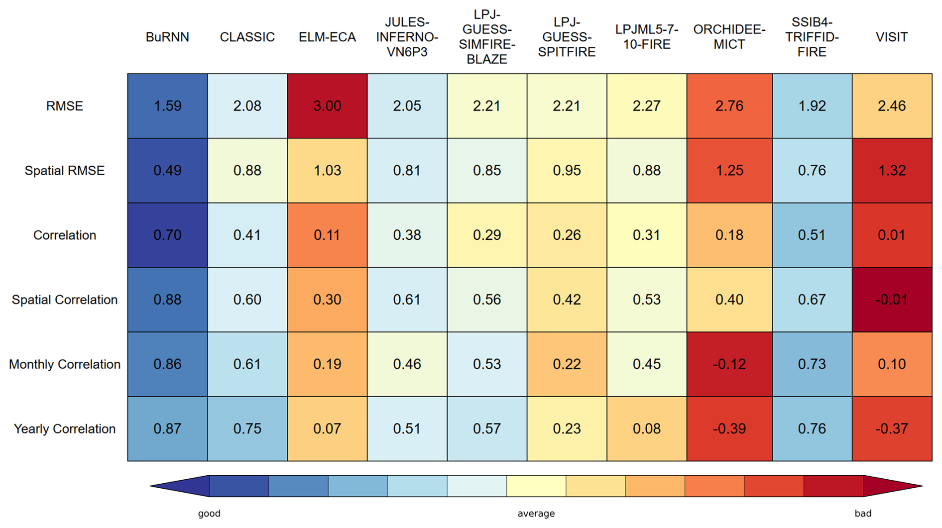
Figure 2 Global evaluation scores of BuRNN and the FireMIP models for 2003–2019. Colour scaling has been done based on the normalized values (value − row mean)$/$(row standard deviation) with the minimum and maximum values set to −2 and 2, respectively. Better scores (lower for RMSE and higher for Pearson correlation) are marked in blue, while worse performance is in red.

We also evaluate our results across 14 fire regions defined by Giglio et al. (2010) in Figs. 6 and 7. Interannual variability is relatively well modelled, although the amplitude is lower than observed for some regions. However, there are differences in performance across regions. Regions such as Temperate North America (TENA), Northern Hemishphere South America (NHSA) and Southern Hemisphere Africa (SHAF) are excellently modelled by BuRNN. In the majority of the regions, BuRNN captures the pattern of the interannual variability well. In the Middle East (MIDE), BuRNN simulates the mean annual burned area well, while the interannual variability and long-term trend are off. In Boreal Asia (BOAS), our model simulates too little burned area, which is likely due to having a similar environmental setting as Boreal North America (BONA) where annual burned area is much lower. In Central Asia (CEAS) and Australia and New Zealand (AUST), interannual variability is reasonably modelled, but the highest burning years are underestimated e.g., 2001–2008 in CEAS and 1998–2002 in AUST. Global annual burned area is mostly dominated by the (African) savannah regions; therefore the ability of BuRNN to capture mean burned area, interannual variability and long-term trend is reflected in the good global performance Table A2. In most regions BuRNN outperforms the process-based fire models over most metrics (Table 3). Lastly, we compare the distributions of observed and modelled burned area Fig. A23. We note that the rare high burned areas (>50 % of land surface area) are generally not modelled by BuRNN.

Next, we repeat this evaluation procedure using the 2001–2019 FireCCI51 observational dataset as reference. We do this because our model is specifically trained to predict GFED5 burned area, while the process-based models are not. Although the absolute values between FireCCI51 and GFED5 differ, a similar pattern as Table 3 is observed when comparing BuRNN and the process-based models against FireCCI51 (Table A8). BuRNN tends to outperform the process-based models, although less strongly than before. Especially the in the 3D RMSE BuRNN is often not the best performing model anymore. This makes sense as total burned area in FireCCI51 is about half of GFED5 so BuRNN is expected to make larger errors. In the correlation metrics however, BuRNN still clearly outperforms the process-based models most of the time. There are two regions/metrics for which the FireCCI51 and GFED5 observational products show notable differences (Table A3). First the yearly correlation for Southeast Asia (SEAS) between the two observational products is only 0.42. Second, the 3D correlation in Central America (CEAM) is only 0.58, notably lower than all other regions and similar to the 3D correlation in Equatorial Asia (EQAS). Therefore, any (dis)similarity of any model with any observational product should be taken with relatively large observational uncertainty in mind.

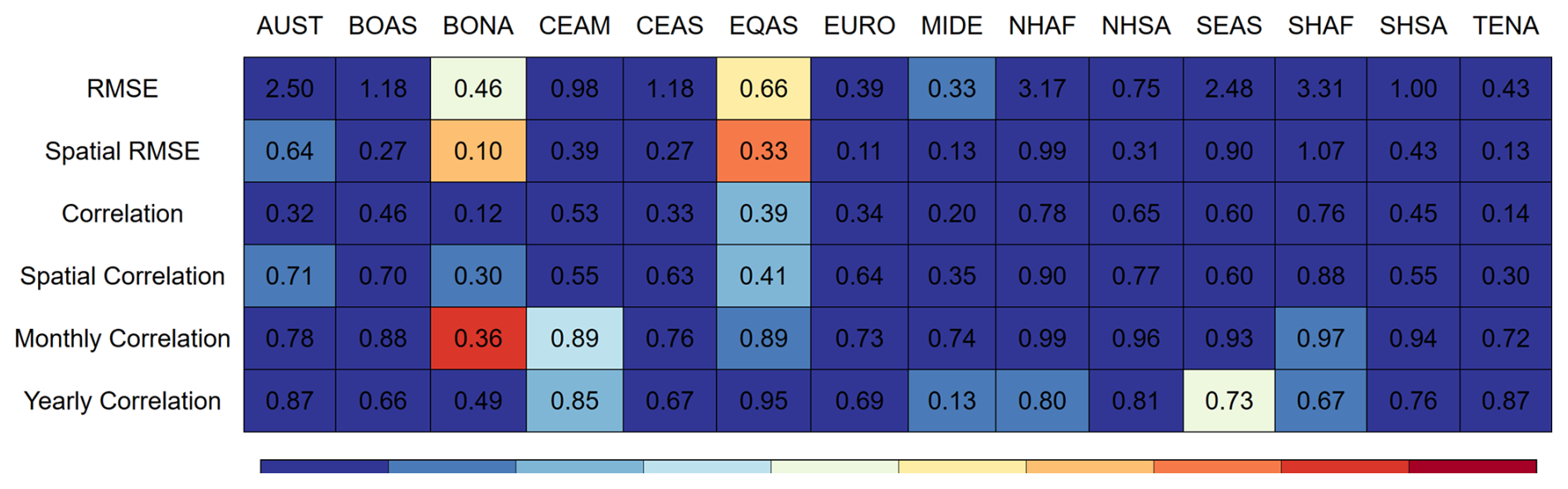
Figure 3 Regional evaluation scores of BuRNN. Colour scaling has been done based on the ranked values compared to the nine process-based fire models, with the minimum RMSE and maximum correlations coloured blue (best) and the highest RMSE and lowest correlation coloured red (worst).

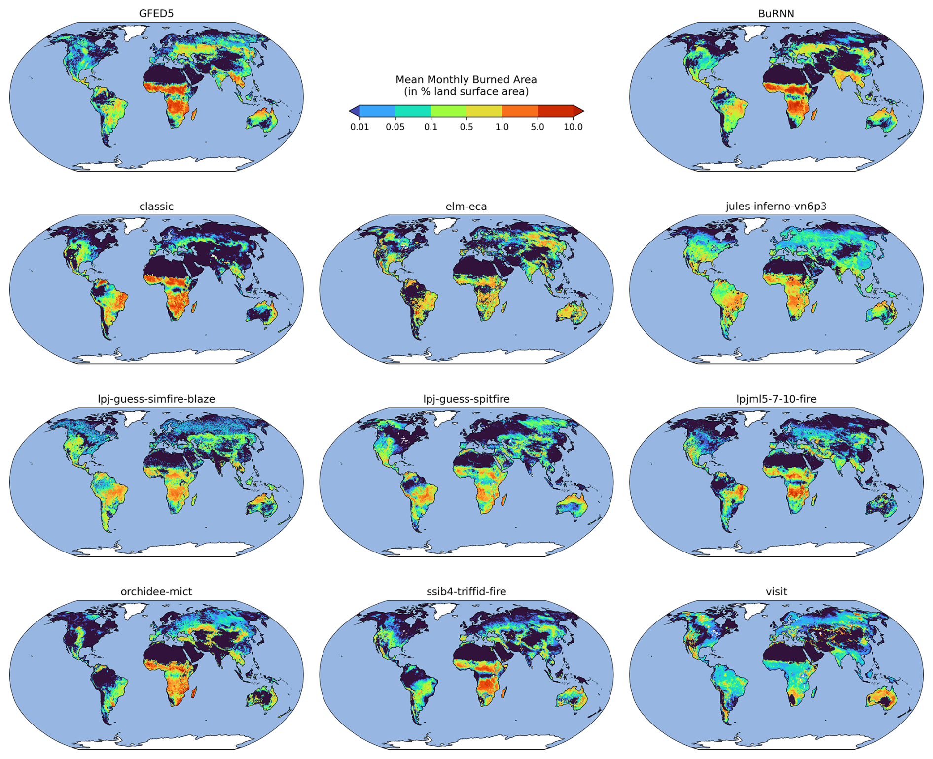
Figure 4 Mean monthly burned area (in % land surface area) over 1997–2019 for the GFED5 satellite product, BuRNN and the nine FireMIP models.

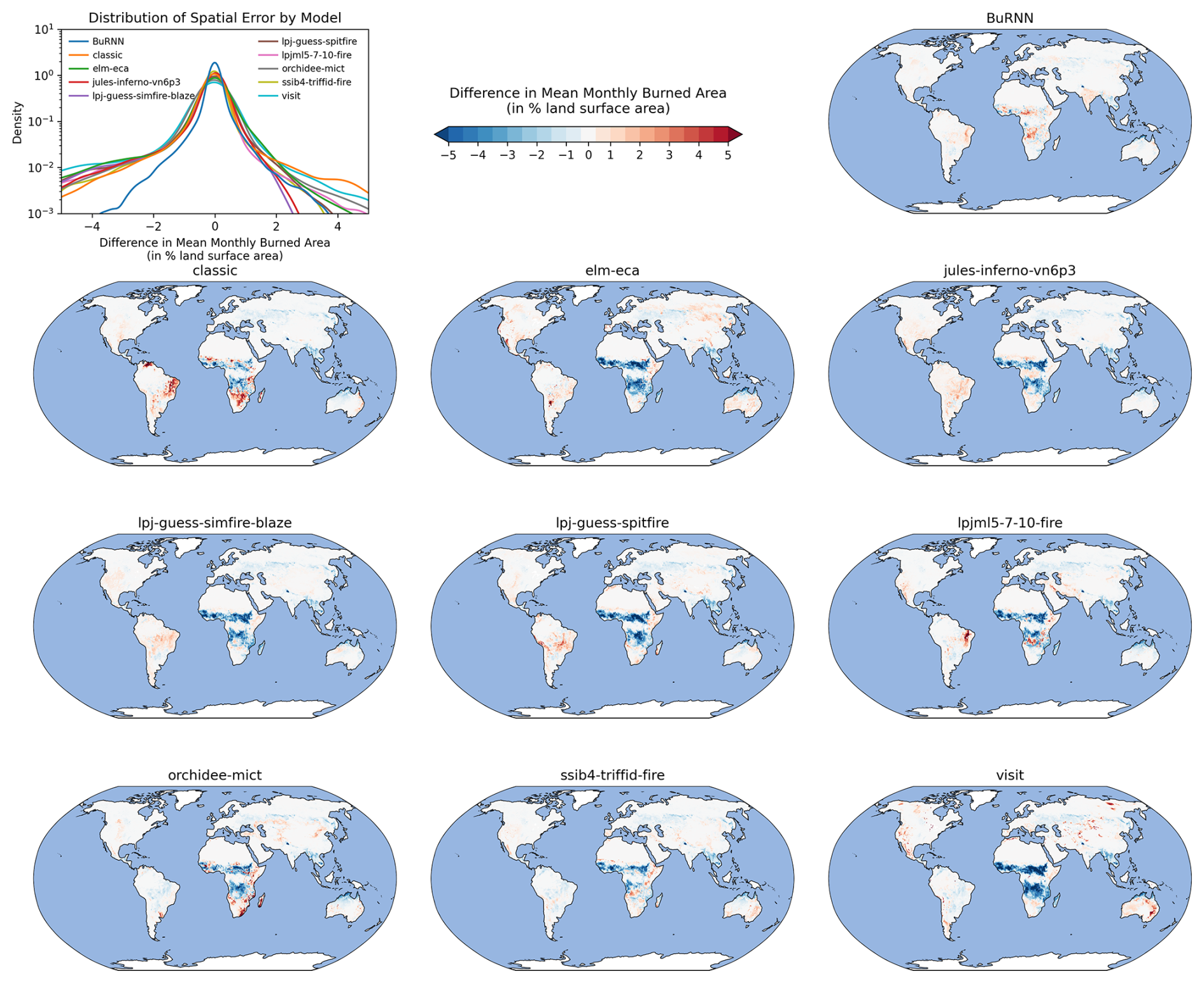
Figure 5 Spatial difference in mean monthly burned area (in % land surface area) over 1997–2019 between GFED5 and the model simulations (including BuRNN). The left upper panel shows the distribution of pixel values per model, the more closely centered around 0, the better the modelled burned area pattern.

RMSE metrics vary in magnitude across different regions as they have different total burned areas. However, also the correlation metrics show large inter-regional differences. For example, in the MIDE, BuRNN has a very low yearly correlation of 0.13. However, only a single process-based model scores better in this metric. In SEAS, four out of the nine fire models outperform BuRNN in yearly correlation, but BuRNN still has a high correlation of 0.73 in this region. Similar observations can be made over the spatial correlation, where Northern Hemisphere Africa (NHAF) and SHAF are the regions with the best modelled spatial burned area and BONA and TENA the two regions where the spatial pattern is least well modelled of all regions. The likely reason for the lower spatial correlation (both for BuRNN and the process-based models) in these regions is the stochastic nature of fires on these spatial and temporal scales. For example, large regions (many pixels) of Canadian forest are quasi-identical in terms of how their monthly input features look like. In these regions large fires are associated with periods of high fire weather danger, which usually occurs over many pixels on this scale. However, when a large fire event happens only a few pixels will see very high burned areas, where exactly these will occur is difficult to predict. Therefore, BuRNN and many process-based models do not predict these large fires in specific pixels but spread out the burned area over a larger area. This in turn leads to lower spatial predictive power in these regions.

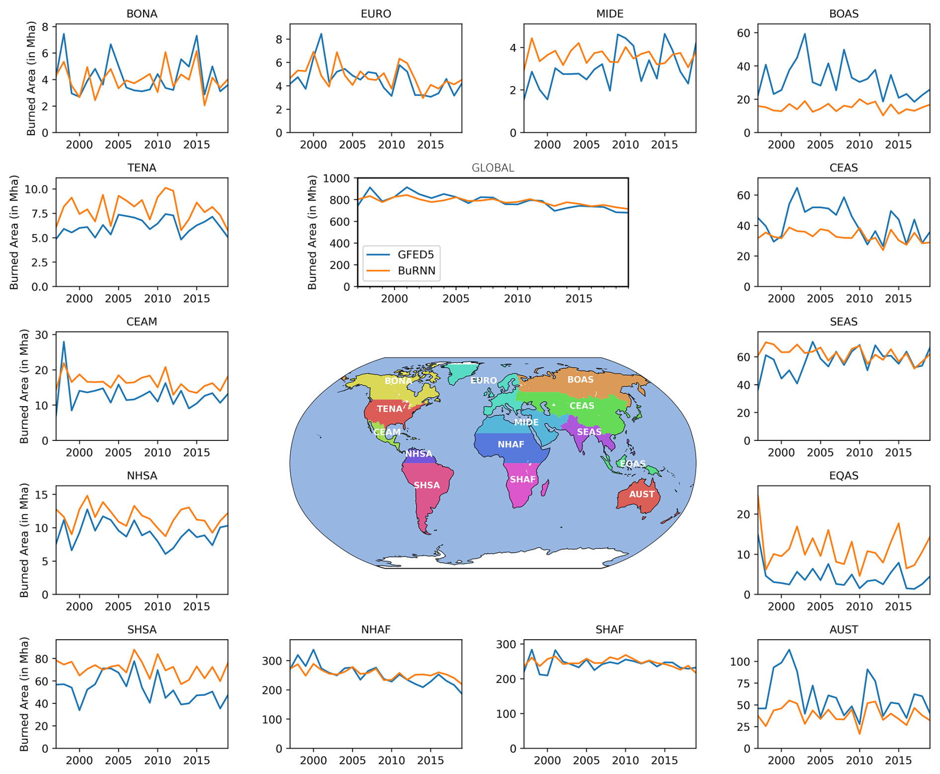
Figure 6 Annual sums (in mHa) of regional burned area by BuRNN (orange) and the GFED5 satellite observations (blue) for 1997–2019. The observed 2003–2019 annual trend is −8.45 ± 3.09 Mha yr⁻¹ (μ± 2 SD), while BuRNN models −4.78 ± 2.21 Mha yr⁻¹.

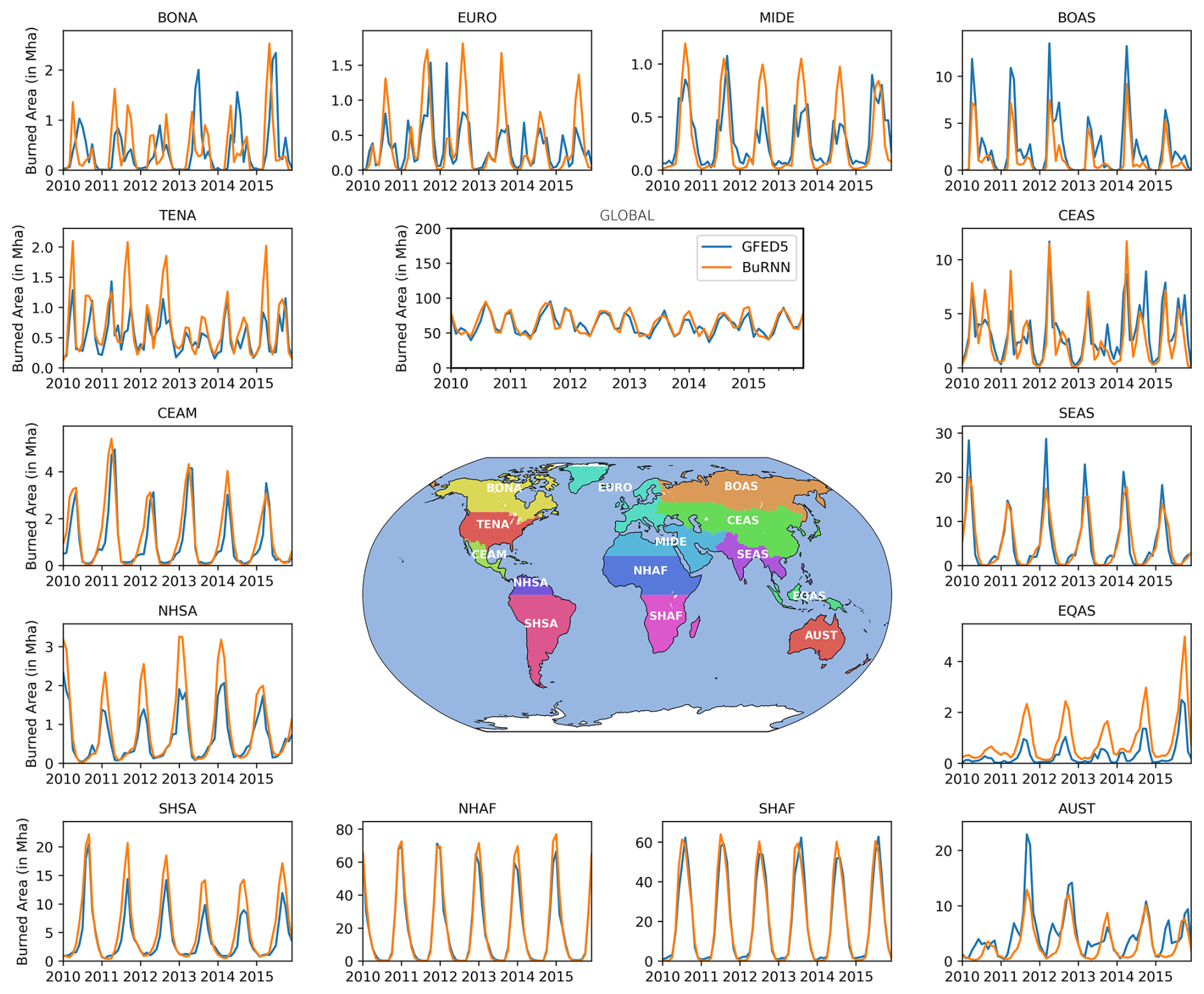
Figure 7 Monthly burned area (in mHa) per region by BuRNN (orange) and the GFED5 satellite observations (blue) for 2010–2015.

3.2 Drivers of BuRNN

We find that the climatic variables FWI and monthly mean of daily maximum temperature (temp) are the most impactful features across all regions (Fig. 8). This suggests that although the Canadian FWI was originally designed to be used in Canadian forests, it can provide relevant information for many, if not all, regions in the world. However, important to consider here is that vegetation characteristics are spread across many more variables, giving each individual vegetation feature a lower importance. Moreover, we see that GDP, a variable often neglected in process-based fire models (Burton et al., 2024), often shows up high in the importance list. We also see bare ground as important indicator in all but one region (EQAS), which is to be expected as a high value of bare ground fraction should immediately render all other features for that grid cell irrelevant. Several regional differences in feature importance can be observed. For example, C₄ grasses show up in regions with considerable grassland/savannah coverage e.g., SHAF, Southern Hemishphere South America (SHSA) and AUST. Needleleaf trees (needletree) only show up in BONA and BOAS, and broadleaf evergreen trees are important in regions with important rainforests e.g., in South-America (NHSA and SHSA) and EQAS. Croplands show up in regions with noteable agricultural burning such as SEAS, EQAS and the MIDE (Hall et al., 2024). Interestingly enough, in Europe (EURO) croplands also are an important indicator, yet Europe does not have as extensive cropland fires as many other regions (Hall et al., 2024). Lastly, monthly average daily wind speed is often not present in the top indicators regionally. Even though wind speed is incredibly important for fire spread, it might (i) be averaged out by the spatial (0.5 by 0.5) and temporal (monthly) scale we are working at, and (ii) it only affects burned area in the month it is actually burning. This is important as we take the average feature importance over many timesteps and hence is likely reduced by this aggregating operation. All of this indicates that BuRNN tends to prioritize specific features in their expected places.

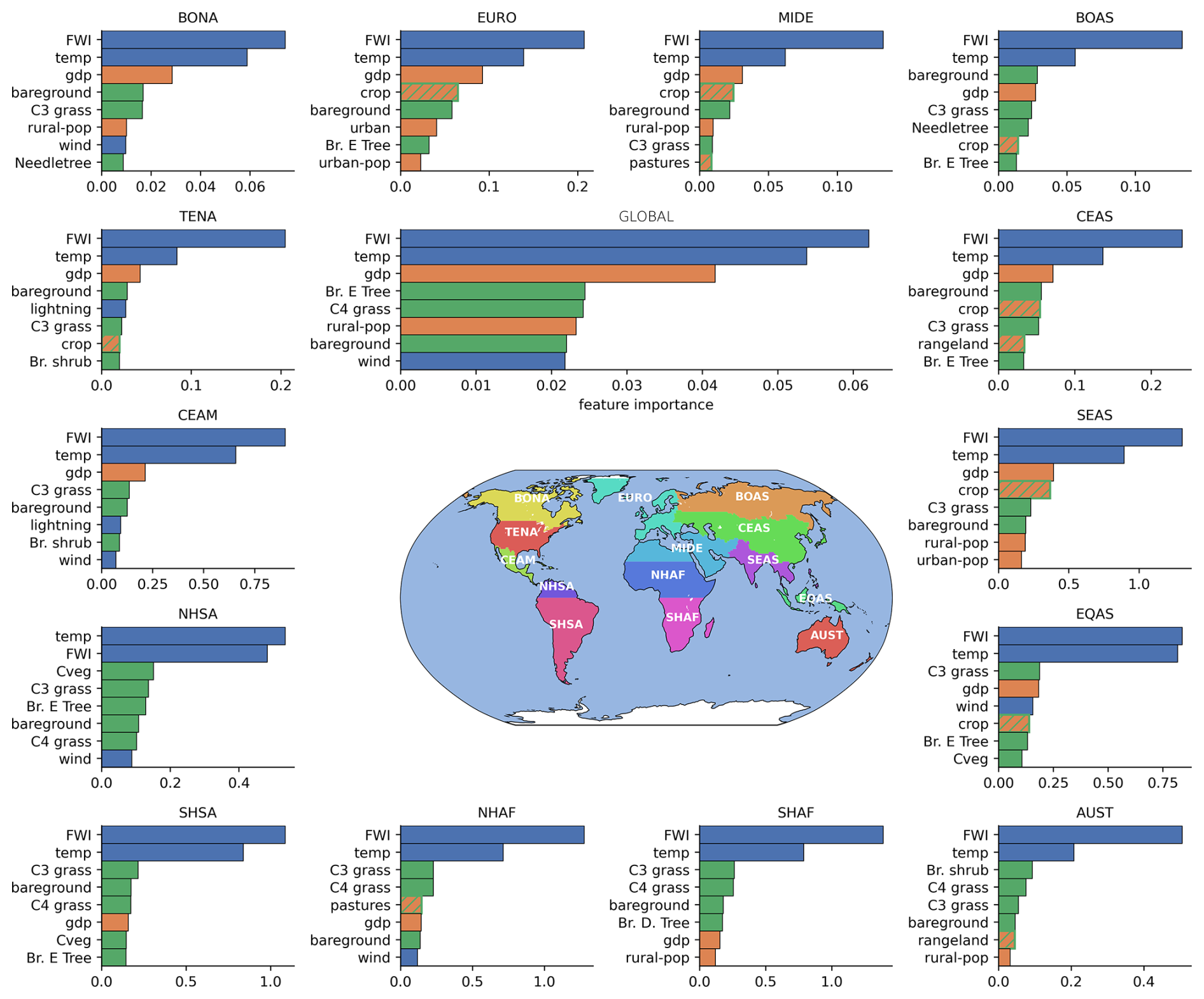
Figure 8 Feature importances for BuRNN per region, indicating which features affect the predictions of BuRNN most in each region. IG attribution values indicate the strength by which a feature affects the prediction of a model compared to that feature's global mean. The top eight are shown for each region, with climate variables in blue, vegetation variables in green and socio-economic variables in orange.

3.3 Application: a burned area reconstruction for the 20th Century

Figure 9 shows the global and regional annual burned area as modelled by BuRNN for the period 1901–2019. BuRNN simulates that globally, from 1901–1960 there has been a slight increase in burned area, which is mainly attributed to an increase in burned area in SHAF in that same period. In TENA BuRNN simulates an increasing trend in burned area from 1901 until ∼ 1955 after which a decline is observed from ∼ 1960 until ∼ 1990. In EURO a first period of high burned area with large interannual variability is modelled from 1901 until ∼ 1950, after which a stark declining trend is modelled by BuRNN. The latter, more recent declining trend is also observed in the EFFIS database. Lastly, for SHAF a positive burned area trend is modelled for the 1901–2010 period, after which burned area again decreases in the last ∼ 10 years. Next, we also want to compare the 1982–1997 part of the BuRNN reconstruction to FireCCiLT11. Figure A2 shows the 1982–2017 regional annual burned area from BuRNN and FireCCiLT11. The annual burned area correlations for 1982–1993 and 1997–2017 between FireCCiLT11 and BuRNN are listed in Table A4 along with the 1997–2017 annual burned area correlations between GFED5 and FireCCiLT11. The annual correlation between the two products is relatively low (0.29). However, the uncertainty in burnt area estimates for this period is relatively high, and on average the correlation between BuRNN and FireCCiLT11 for the early period is higher than between the two observational products themselves for 1997–2017 (Table A4).

Additionally, we compare our reconstruction to regionally available burned area databases. Figure 10 shows the burned area from EFFIS reported by 21 countries in the EU. Both correlation and bias between this EFFIS database and BuRNN is generally high, with BuRNN simulating higher burned areas than EFFIS. We note however that the reported burned area by EFFIS does not include cropland fires, as opposed to BuRNN, explaining part of the absolute bias. In Fig. A3, a further comparison is made for 5 more regions (Canada, US, Brazil, Chile and Australia) where the correlation between national databases and BuRNN is only high in Brazil. The likely explanation for this discrepancy lies in the data collection. Correlation between BuRNN and EFFIS is high for individual countries, but is close to 0 when assessed over the 21 European countries combined for the entire period. As each national dataset inside the EFFIS database has a different start and end date, it makes calculating interannual variability inconsistent (unless we restrict the database to only those years available in all countries, which is 2017–2019). Similarly, many of the other national databases, like those in Canada, US and Australia, are composed of regional data sources that come available in different time periods mixed in with satellite images (usually LandSat) when available. In contrast, MapBiomas in Brazil has a single data source (LandSat) and thus does not suffer from this, there correlation (1985–1996) with BuRNN is high (0.74). Therefore, we believe BuRNN shows a good correlation with these independent data sources whenever the data sources have consistent reporting of burned area. Moreover, in Europe a decreasing trend in annual burned area has been reported, especially in the Mediterranean (Rodrigues et al., 2013; Turco et al., 2016; Chen et al., 2023b). This is in line with the reconstruction of BuRNN.

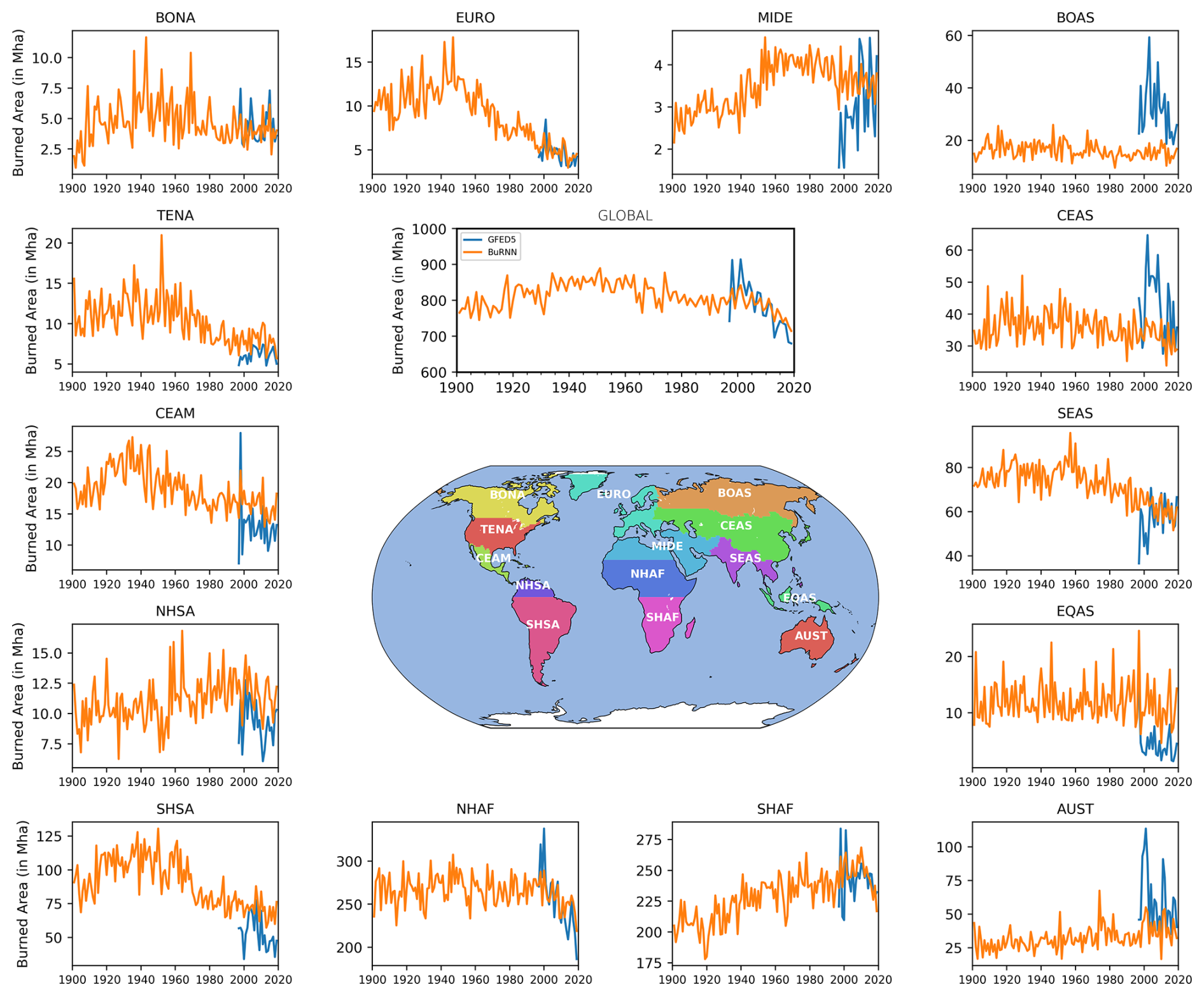
Figure 9 BuRNN's simulation of total annual burned burned area (in Mha) from 1901 to 2019 (orange) for each of the fourteen GFED5 regions and globally, along with the 1997–2019 GFED5 satellite-based burned area.

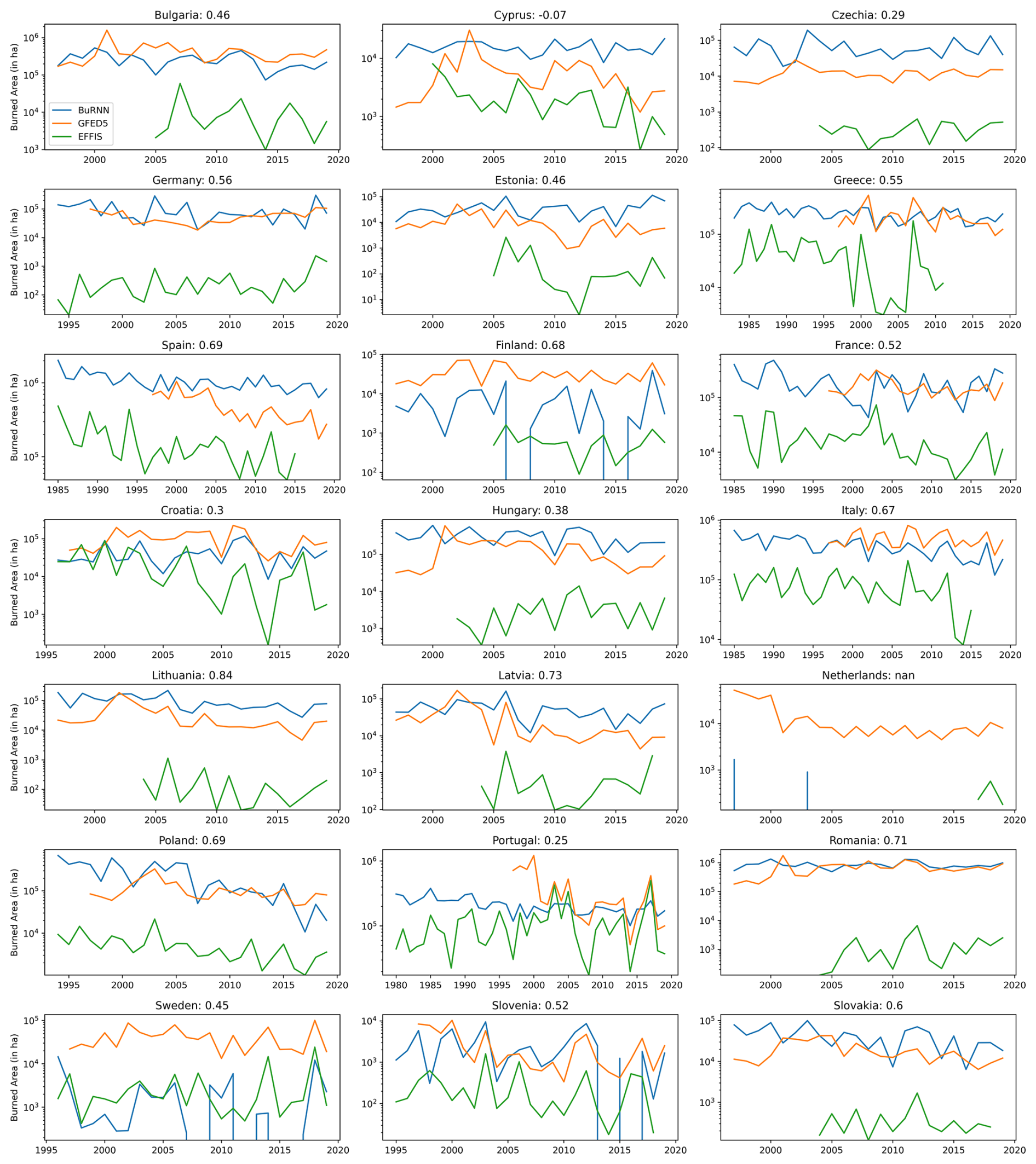
Figure 10 Annual sums (in ha) of national burned area by BuRNN (orange) and as reported by EFFIS. Methods for collecting and reporting burned area differ by country (and may differ throughout time), the periods for which data have been plotted are between 1983 and 2019. Note that EFFIS does not include cropland fires.

4 Discussion

Scientific performance aside, BuRNN has a second benefit compared to process-based models i.e., speed and cost of running the model. Running the full 1901–2019 reconstruction (for all the 55 models) takes approximately an hour in total on a single CPU core on our HPC cluster. This is in stark contrast to the computational cost required to run fire-coupled DGVMs, which require hundreds up to tens of thousands of CPU hours. Of course, the major cost of running BuRNN is in the training phase, which typically takes around 10 h on a single GPU (NVIDIA GeForce 1080Ti). Although the speed and performance of this first version of BuRNN are excellent, it does come at the expense of interpretability. As with most deep learning architectures, BuRNN does not physically relate drivers to responses. We have done effort to alleviate this through our XAI analysis, which approximates feature importance, but this understanding is not on par with our knowledge of the mechanisms in process-based models. Conversely, data-driven models can potentially contribute to improved process understanding: if we can unravel why and how BuRNN outperforms these process-based fire models, we can leverage that knowledge to improve the process-based models.

During training, we explicitly aimed to prevent overfitting and maximize generalisability in several ways. We employed a region-based cross validation to counteract the high spatial autocorrelation in our data, we used early stopping, applied normalization during preprocessing on the training data, batch normalization after the LSTM layer and dropout after the linear layer. We subsequently evaluated BuRNN in multiple ways over a number of metrics against multiple products. First, we evaluated the performance of BuRNN by assessing its error scores to GFED5, taking into account that for any region in the world, BuRNN has never seen data from that region before. Then we calculated spatiotemporal, spatial and temporal error scores and correlation of BuRNN to GFED5 and FireCCI51. We repeated this for the process-based fire models participating in ISIMIP3a and compared the relative performances, showing that in most regions over most metrics BuRNN outperforms state-of-the-art fire models. Our burned area reconstruction holds major promise for assessing spatial fire patterns in the pre-satellite era. To assess its quality, we compared our 1982–1993 reconstruction to the FireCCiLT11 remote sensing product and national census data. However, the low correlation between GFED5 and FireCCiLT11, highlights important observational uncertainty in the early satellite record, calling for caution when interpreting our AI-based reconstruction relative to FireCCiLT11 in this period. By comparing our reconstruction of BuRNN to national databases wherever available, we can potentially obtain a sense of regional product quality. We find particularly good correlation with national databases in the EU and Brazil. Databases from Canada, US, Chile and Australia showed poor correlation to the BuRNN reconstruction, likely caused by the heterogenous nature of these reference datasets. However, three main sources of uncertainty and drawbacks need to be raised. First, our model will learn relationships between population densities, GDP and fire occurrence. These might have changed over the last 120 years and nor BuRNN, nor the process-based models can account for this currently. Secondly, BuRNN also relies on three inputs from DGVMs, which are of course reliant on the performance of the model ensembles for these variables. Lastly, in BuRNN there are currently no fire-vegetation feedbacks, which are present in most process-based models.

5 Conclusions

Compared to process-based fire models, BuRNN pushes the state of the art in terms of simulation quality of burned area, demonstrating the potential for machine learning to improve the predictive capabilities in regional-to-global scale fire modelling. As fire behaviour is expected to have changed and continue to change due to climate change, understanding how they have evolved and will evolve is important for understanding our ecosystems, emissions and land use changes. BuRNN substantially improves our capabilities for simulating fire behaviour in all regions of the world compared to state-of-the-art process-based fire models. However, as a machine learning model its interpretability remains below that of conventional fire models. To address this limitation, we applied XAI to unravel some of the inner workings of BuRNN. From this, we conclude that in most regions, BuRNN prioritizes features that are relevant for that region. This includes, for example, FWI and temperature in all regions, C₄ grasses in regions with notable savannah areas and tree subtypes in regions with extensive forests. As an application, we apply BuRNN to reconstruct global monthly burned area at 0.5°×0.5° spatial resolution over the period 1901–2019. While a valuable dataset for studying historical burned area patterns, it is a challenge to assess the quality of the product, given considerable discrepancy between different satellite-based burned area products and between the satellite products and national inventories. As the effects of climate change and socio-economic drivers on fire behaviour are largely unknown (quantitavely), BuRNN can aid in better unravelling past burned area patterns, which can improve carbon cycle modelling, help fire risk prevention and inform policy makers.

Appendix A

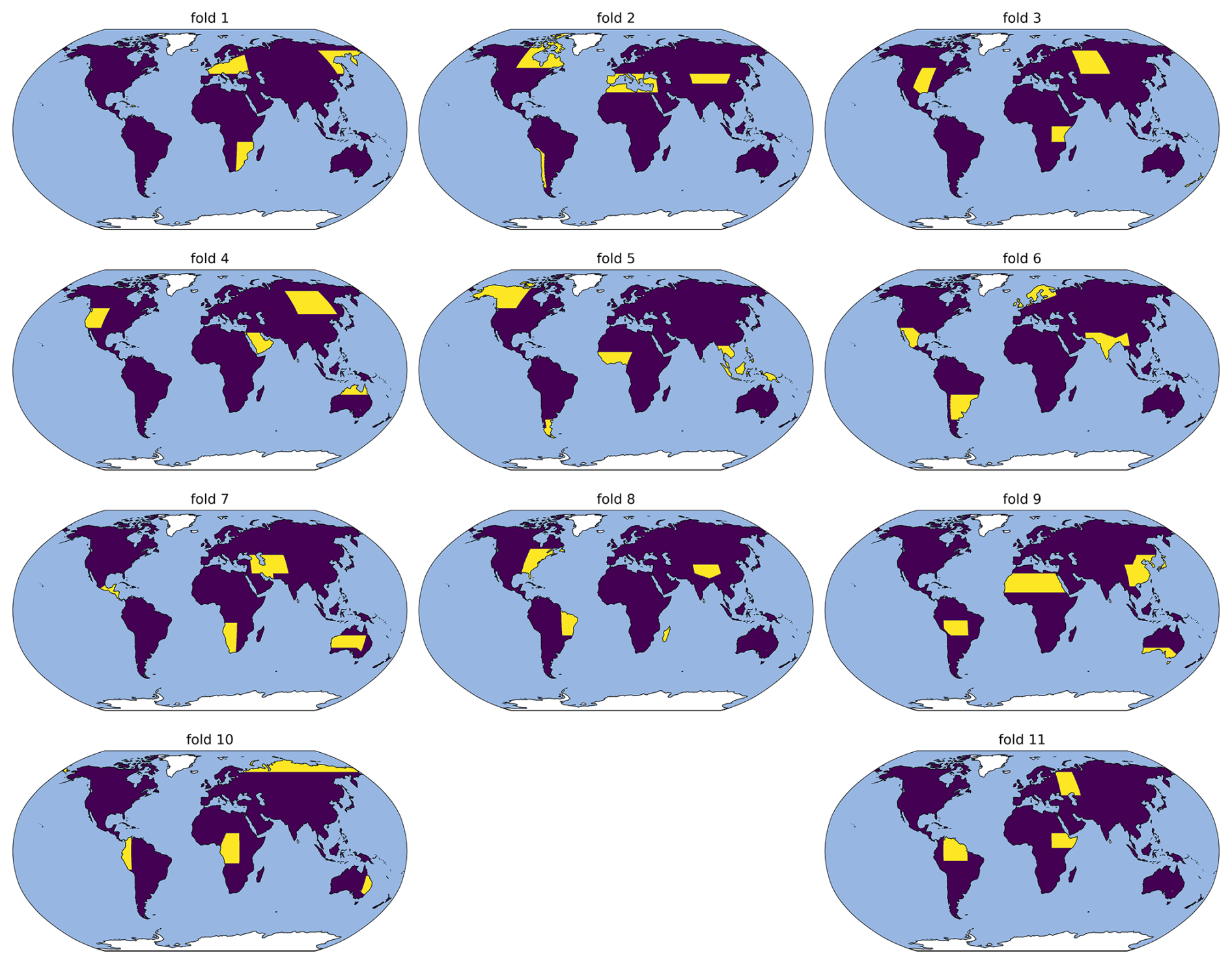
Figure A1 Division of the 43 regions into 11 folds, used for training the models. The regions marked in yellow represent the 3–4 AR6 regions in that fold. During training we set each fold aside once, then train 5 models on the remaining 10 folds, each time with 8 folds as training and 2 folds as validation. E.g., Fold 1 is set aside as testing fold, then folds 2–3 are used as validation and folds 4–11 as training. Then, folds 4–5 are used as validation and folds 2–3 and 6–11 as training. This is followed by folds 6–7 as validation and folds 2–5 and 8–11 as training, etc.”

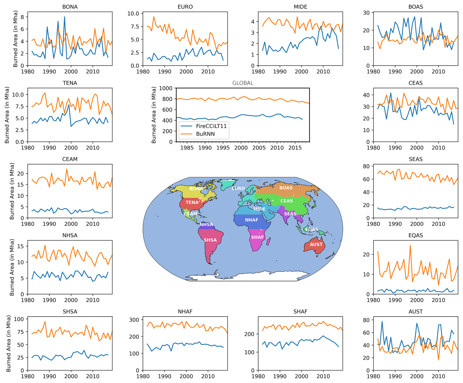
Figure A2 Annual sums of regional burned area by BuRNN (orange) and the FireCCiLT11 observations (blue) for 1982–2018.

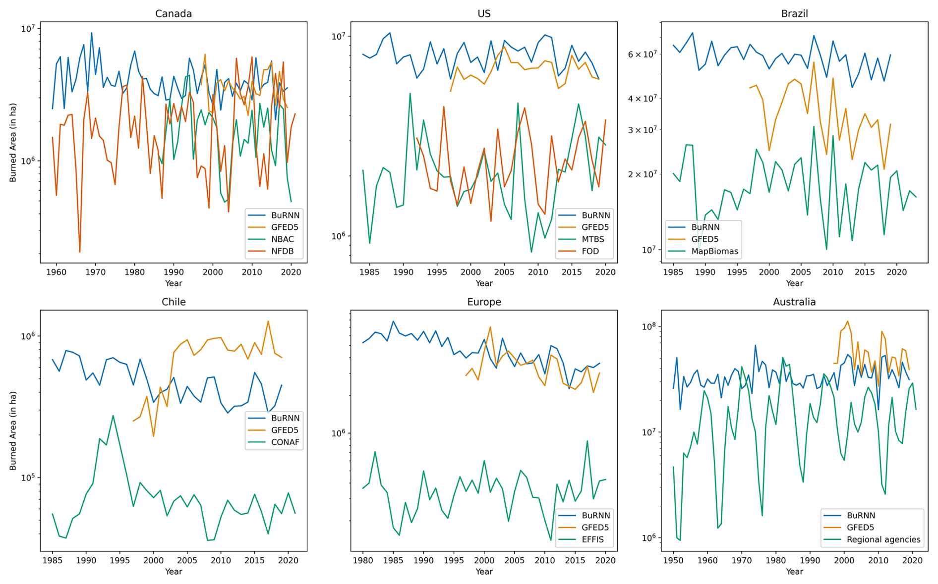
Figure A3 Comparison of BuRNN to regional burned area databases. Note that in some regions managed and/or agricultural fires are not reported.

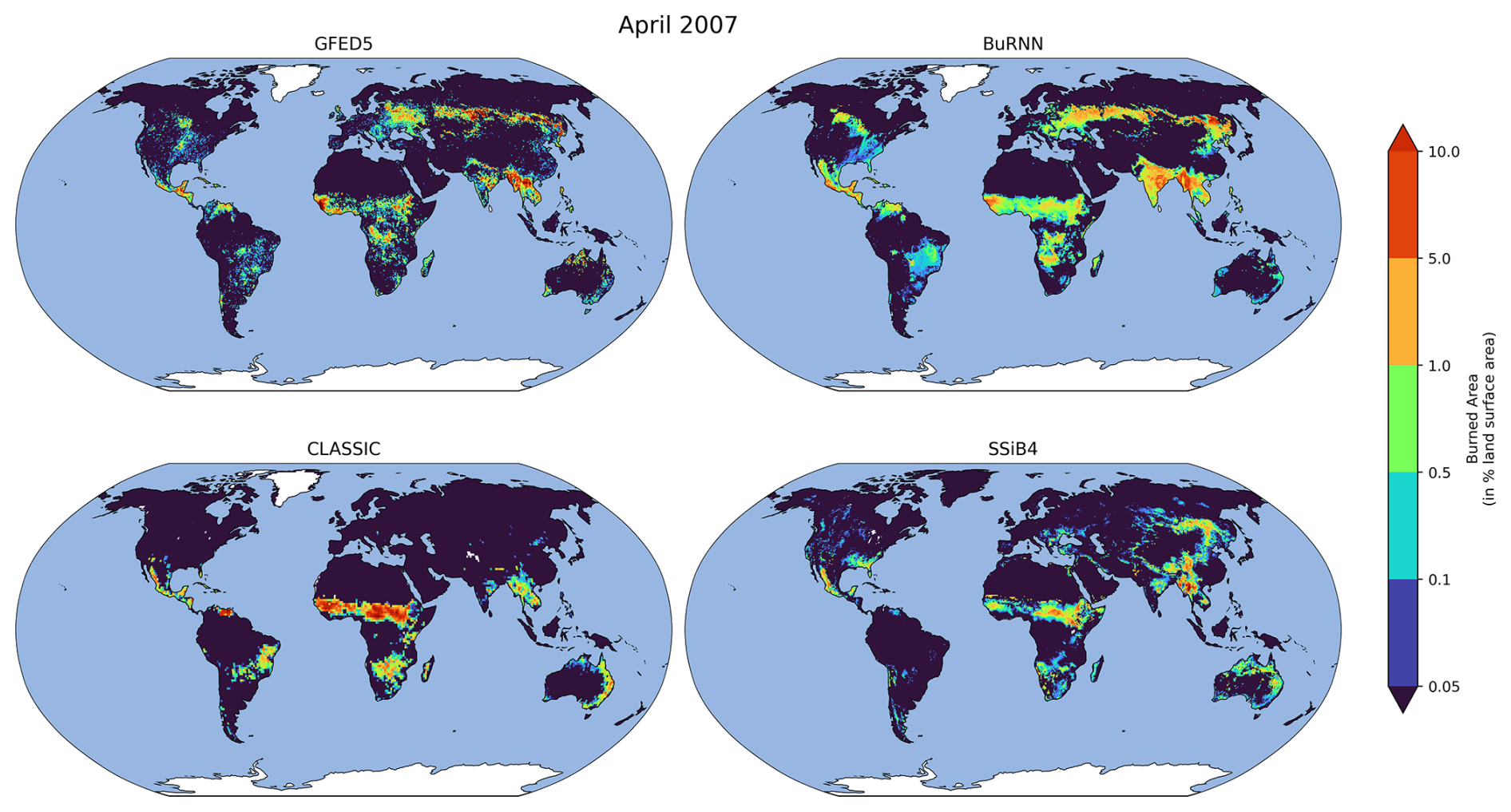
Figure A4 Comparison of BuRNN to GFED5 along with two process-based models (SSiB4 and CLASSIC) for April 2007.

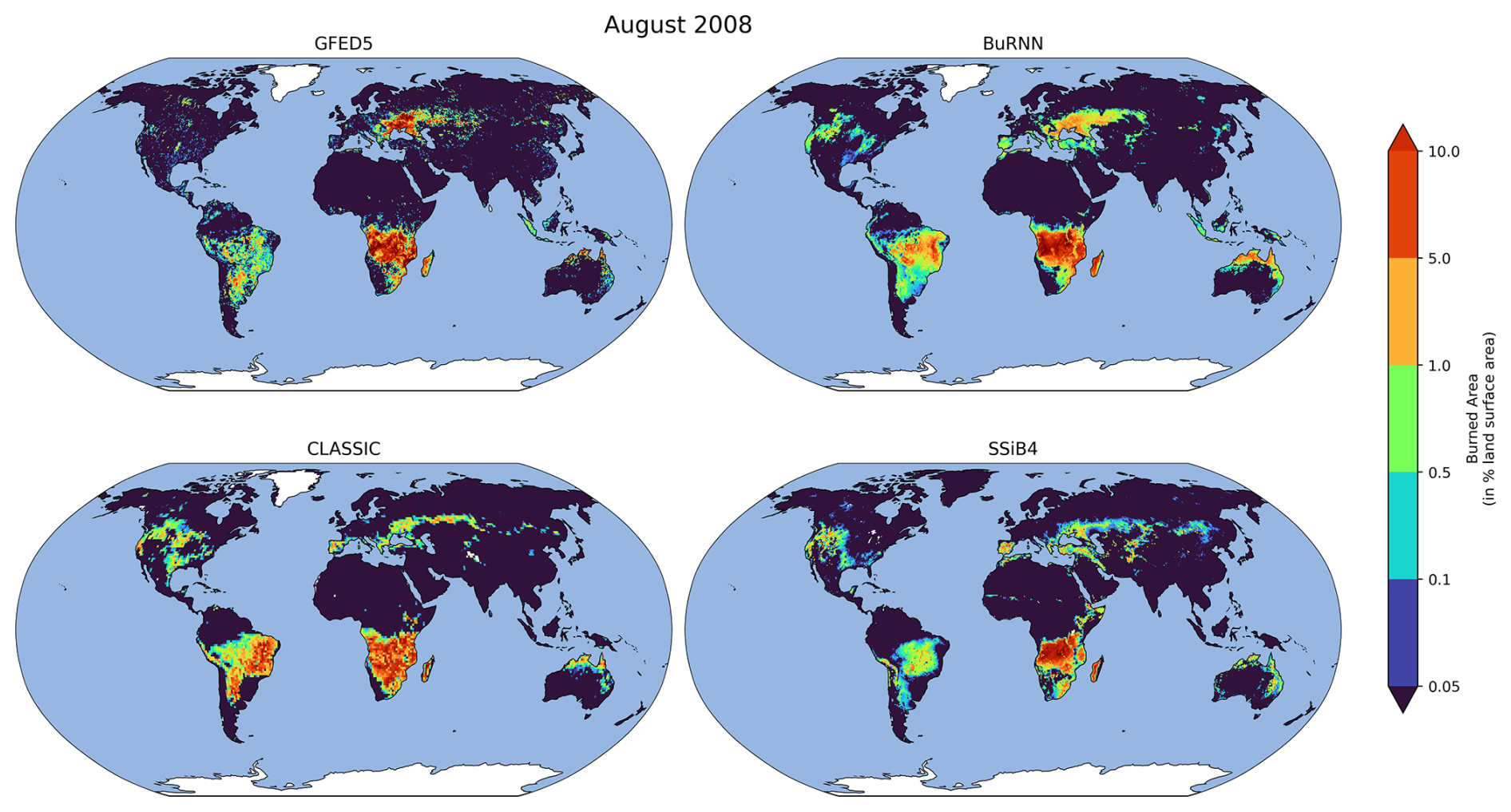
Figure A5 Comparison of BuRNN to GFED5 along with two process-based models (SSiB4 and CLASSIC) for August 2008.

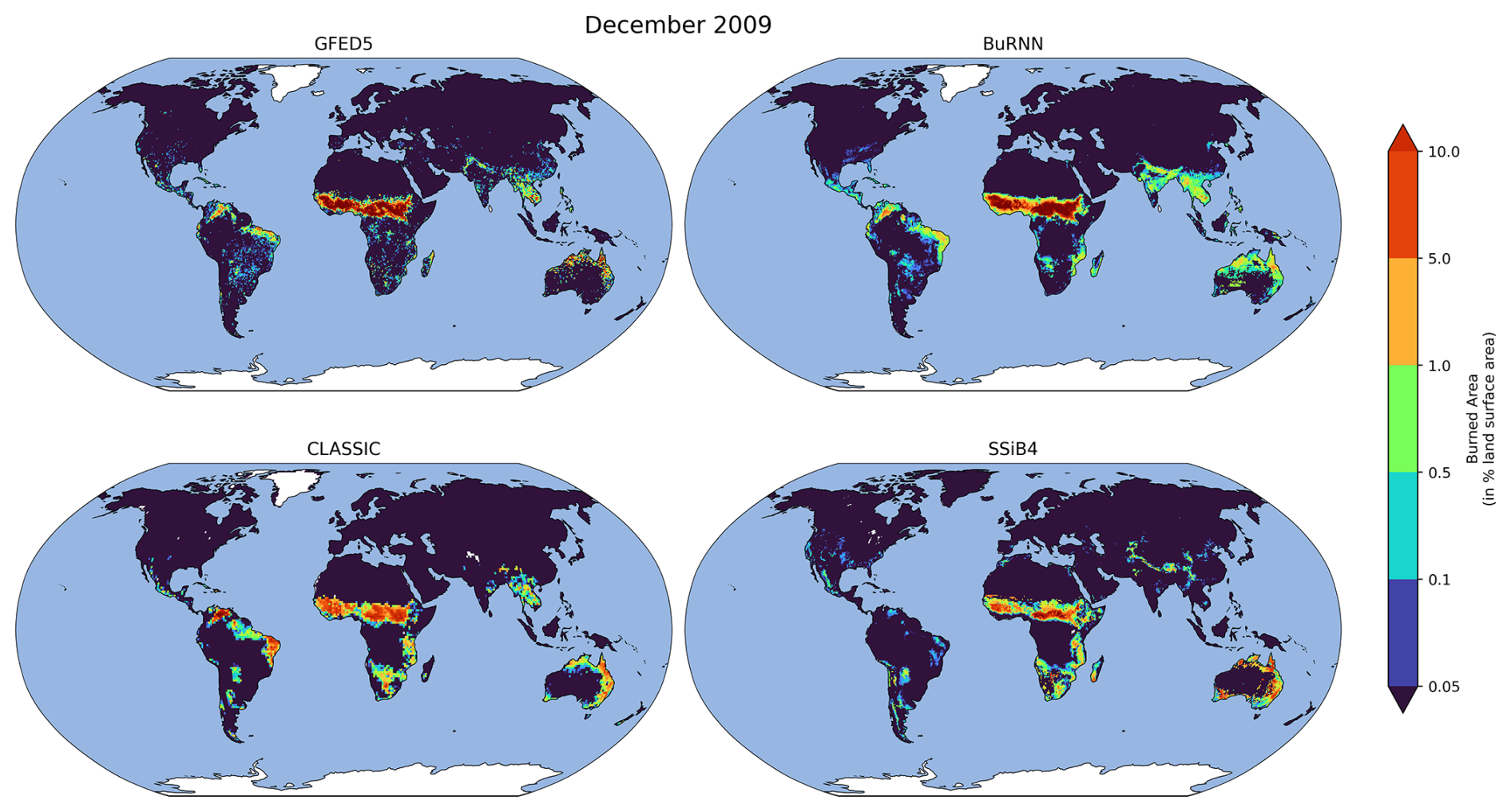
Figure A6 Comparison of BuRNN to GFED5 along with two process-based models (SSiB4 and CLASSIC) for December 2009.

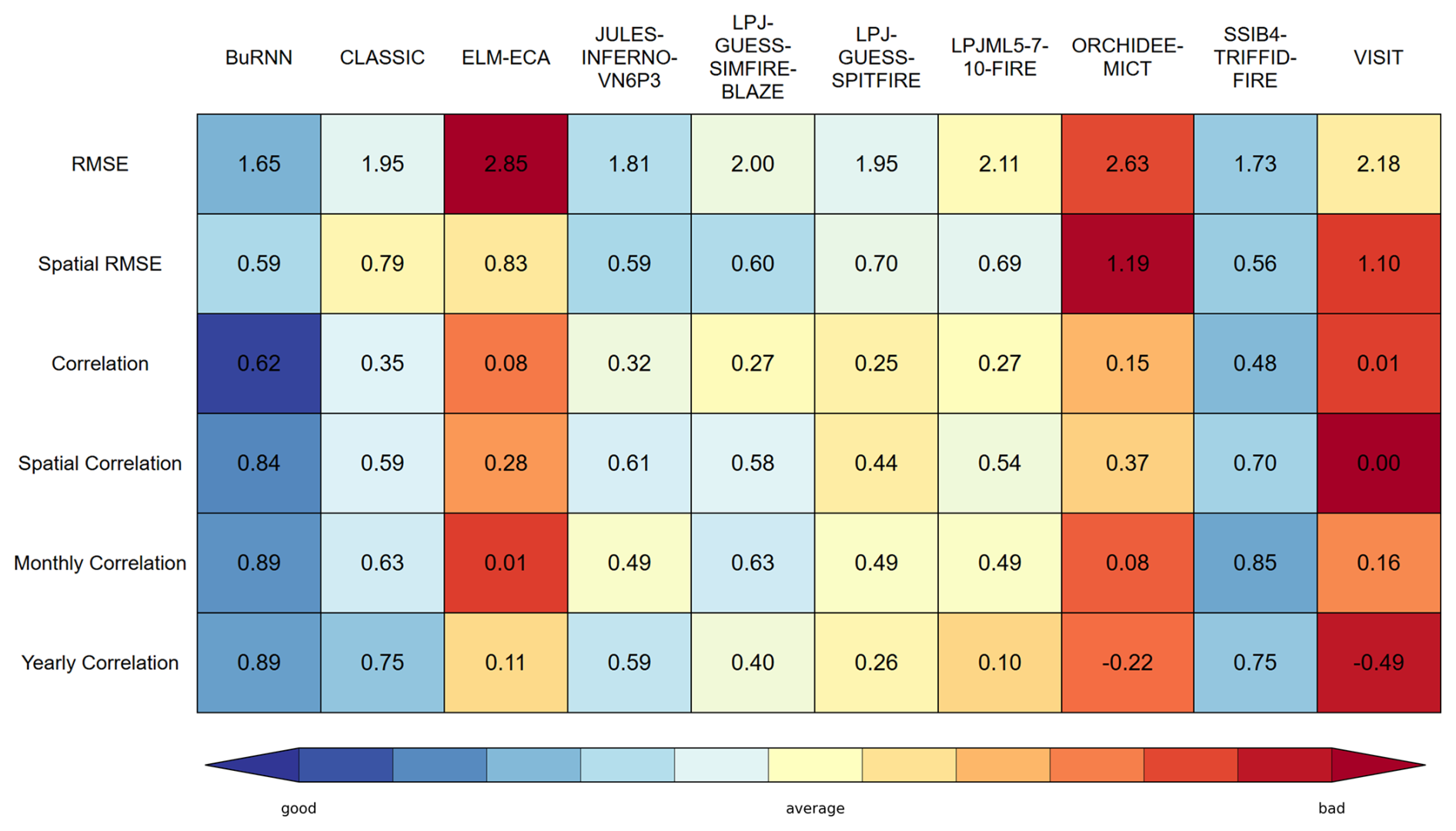
Figure A7 Global evaluation scores of BuRNN and the FireMIP models compared to FireCCI51 for 2003-2019. Colour scaling has been done based on the normalized values (value − row mean)$/$(row standard deviation) with the minimum and maximum values set to −2 and 2, respectively. Better scores (lower for RMSE and higher for Pearson correlation) are marked in blue, while worse performance is in red.

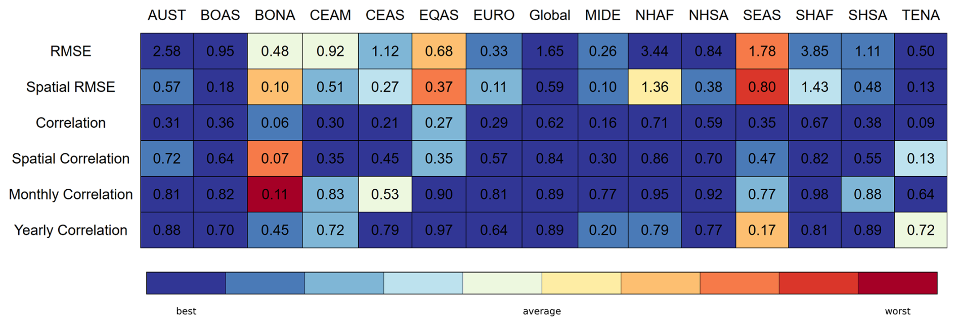
Figure A8 Regional evaluation scores of BuRNN compared to FireCCI51 for 2003–2019. Colour scaling has been done based on the ranked values compared to the nine process-based fire models, with the minimum RMSE and maximum correlations coloured blue (best) and the highest RMSE and correlation coloured red (worst).

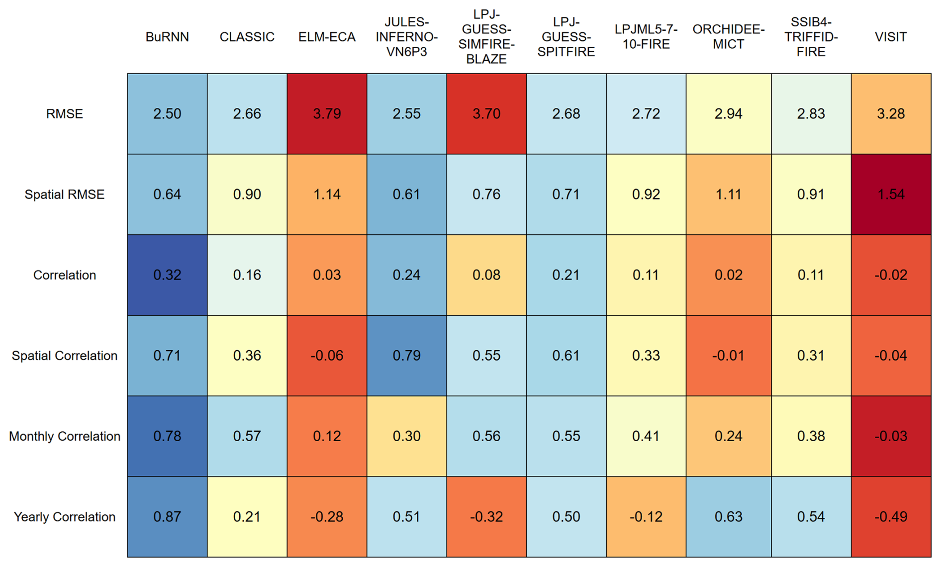
Figure A9 Evaluation scores of BuRNN and the FireMIP models in AUST. Colour scaling is based on the normalized values with the minimum and maximum values set to −2 and 2 (σ). Better scores are marked in blue, while worse performance is in red.

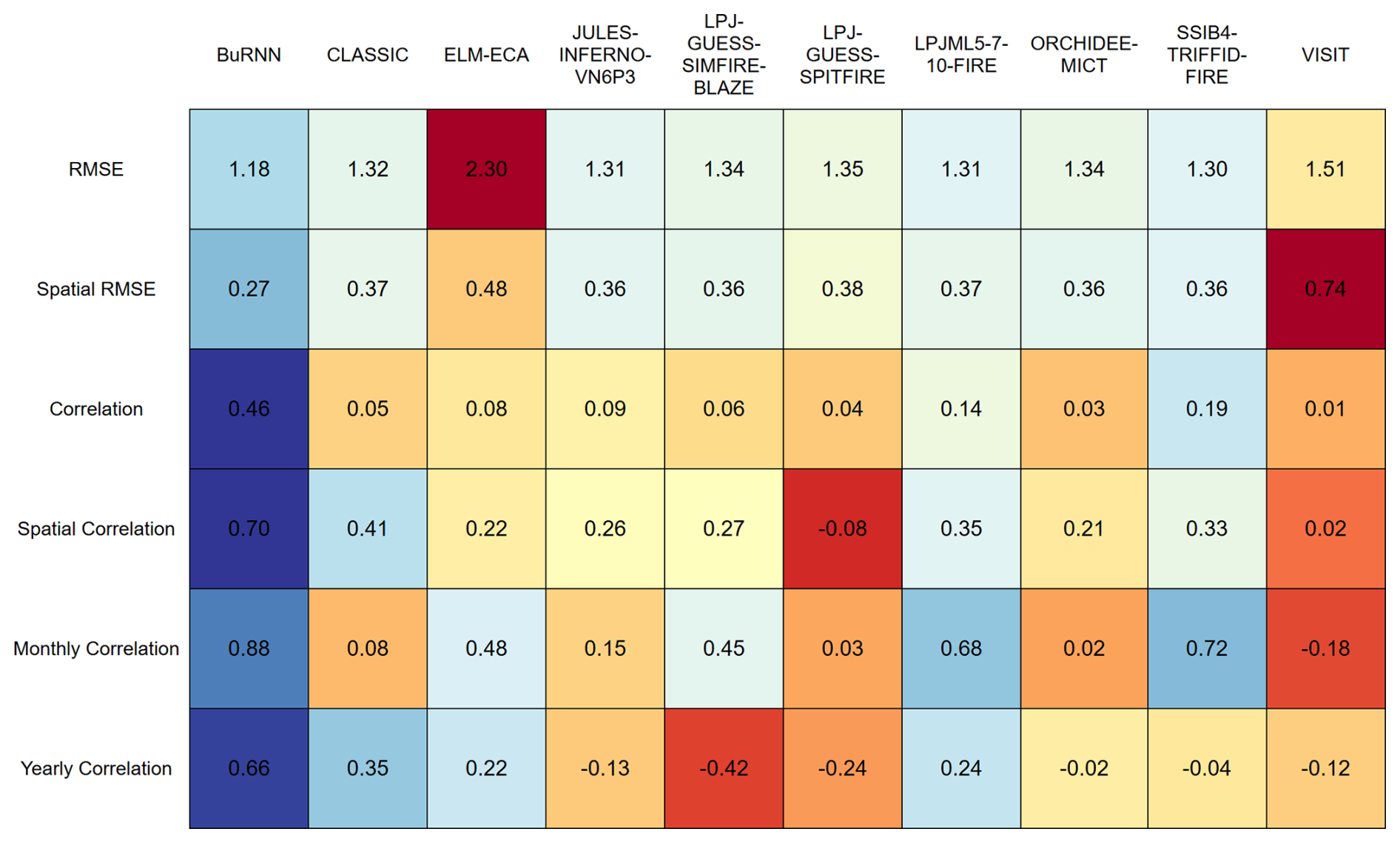
Figure A10 Evaluation scores of BuRNN and the FireMIP models in BOAS. Colour scaling is based on the normalized values with the minimum and maximum values set to −2 and 2 (σ). Better scores are marked in blue, while worse performance is in red.

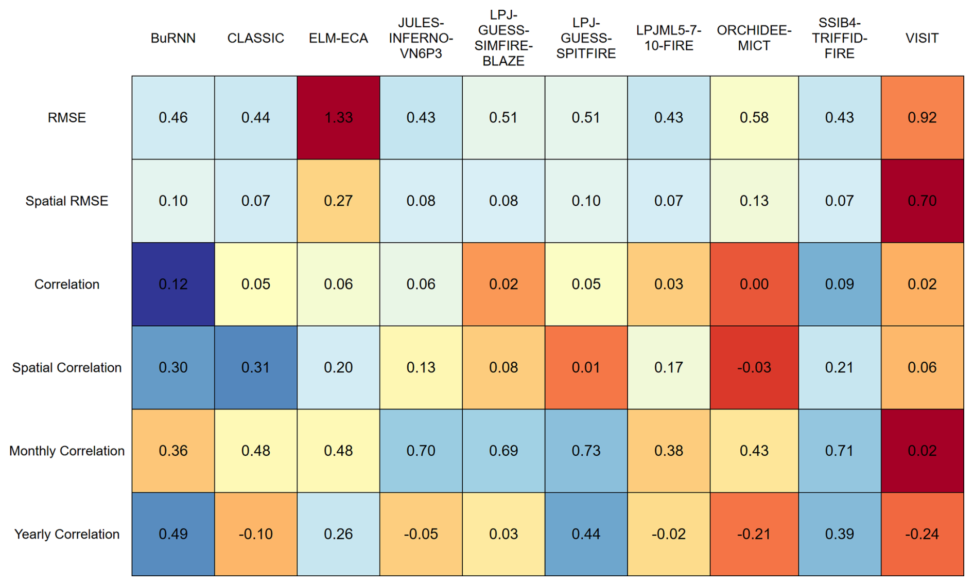
Figure A11 Evaluation scores of BuRNN and the FireMIP models in BONA. Colour scaling is based on the normalized values with the minimum and maximum values set to −2 and 2 (σ). Better scores are marked in blue, while worse performance is in red.

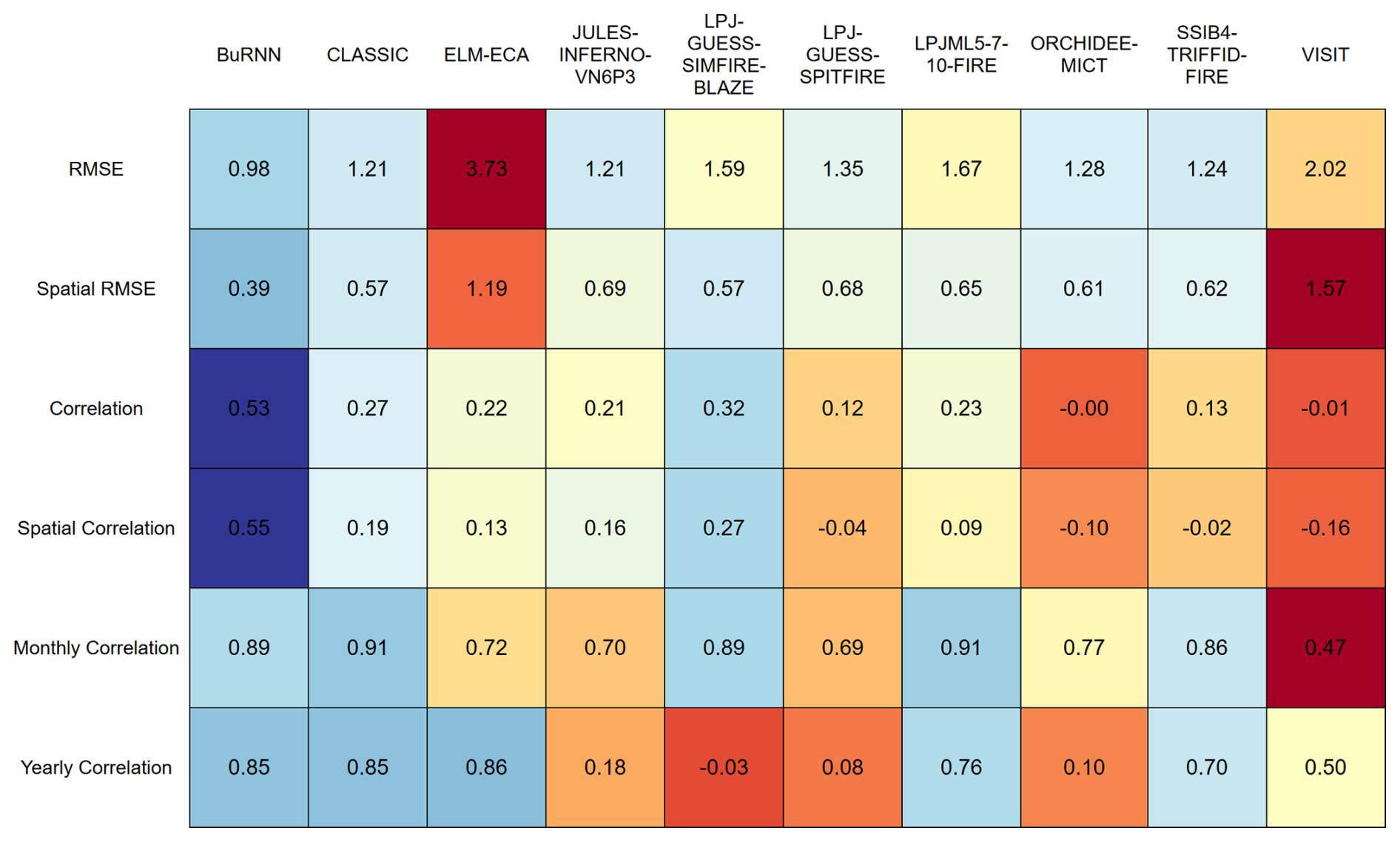
Figure A12 Evaluation scores of BuRNN and the FireMIP models in CEAM. Colour scaling is based on the normalized values with the minimum and maximum values set to −2 and 2 (σ). Better scores are marked in blue, while worse performance is in red.

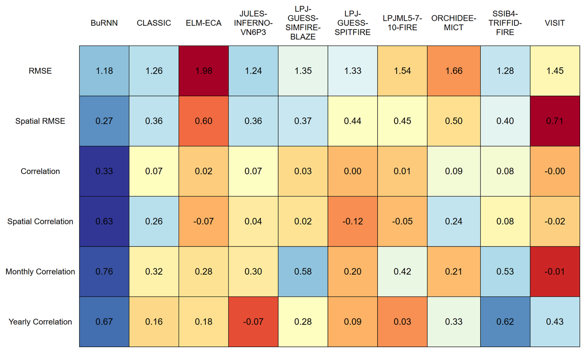
Figure A13 Evaluation scores of BuRNN and the FireMIP models in CEAS. Colour scaling is based on the normalized values with the minimum and maximum values set to −2 and 2 (σ). Better scores are marked in blue, while worse performance is in red.

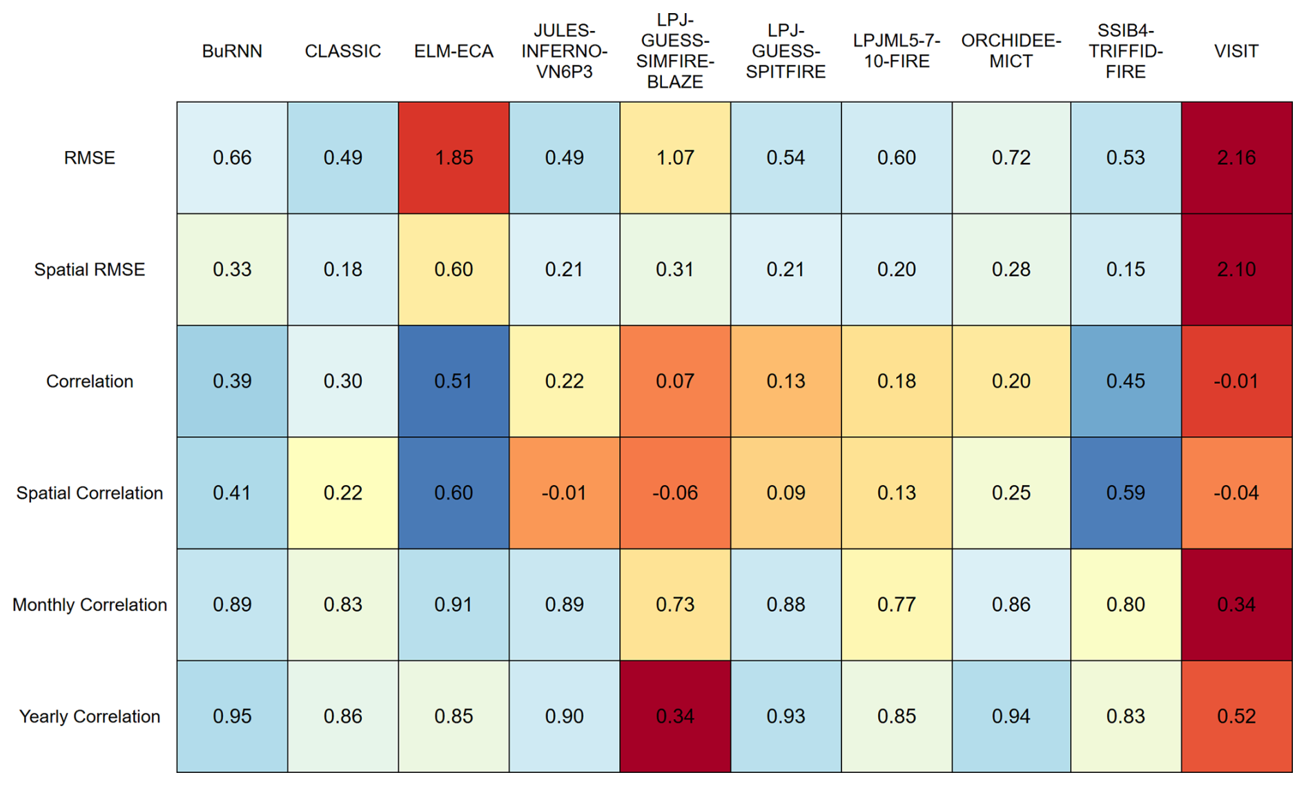
Figure A14 Evaluation scores of BuRNN and the FireMIP models in EQAS. Colour scaling is based on the normalized values with the minimum and maximum values set to −2 and 2 (σ). Better scores are marked in blue, while worse performance is in red.

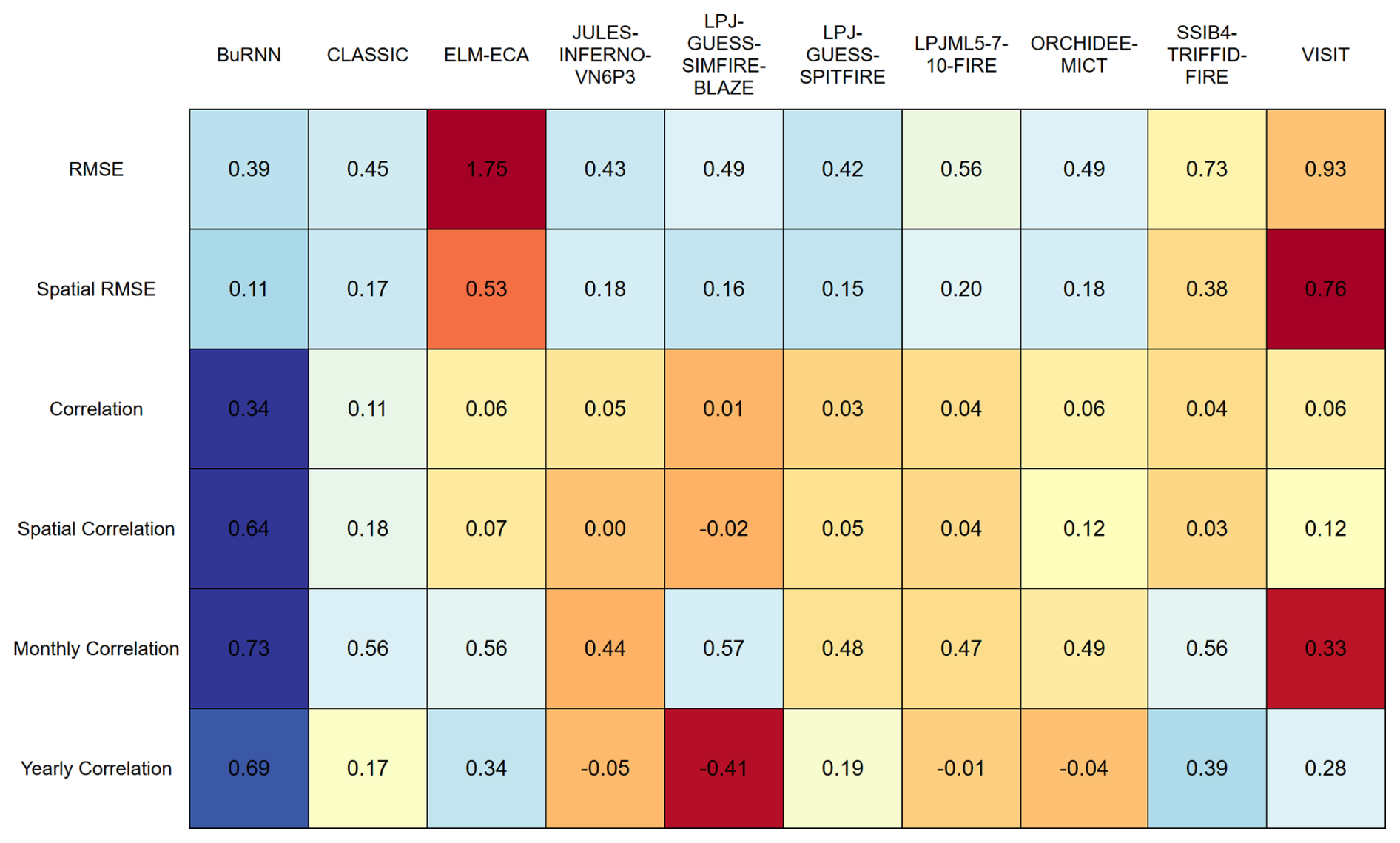
Figure A15 Evaluation scores of BuRNN and the FireMIP models in EURO. Colour scaling is based on the normalized values with the minimum and maximum values set to −2 and 2 (σ). Better scores are marked in blue, while worse performance is in red.

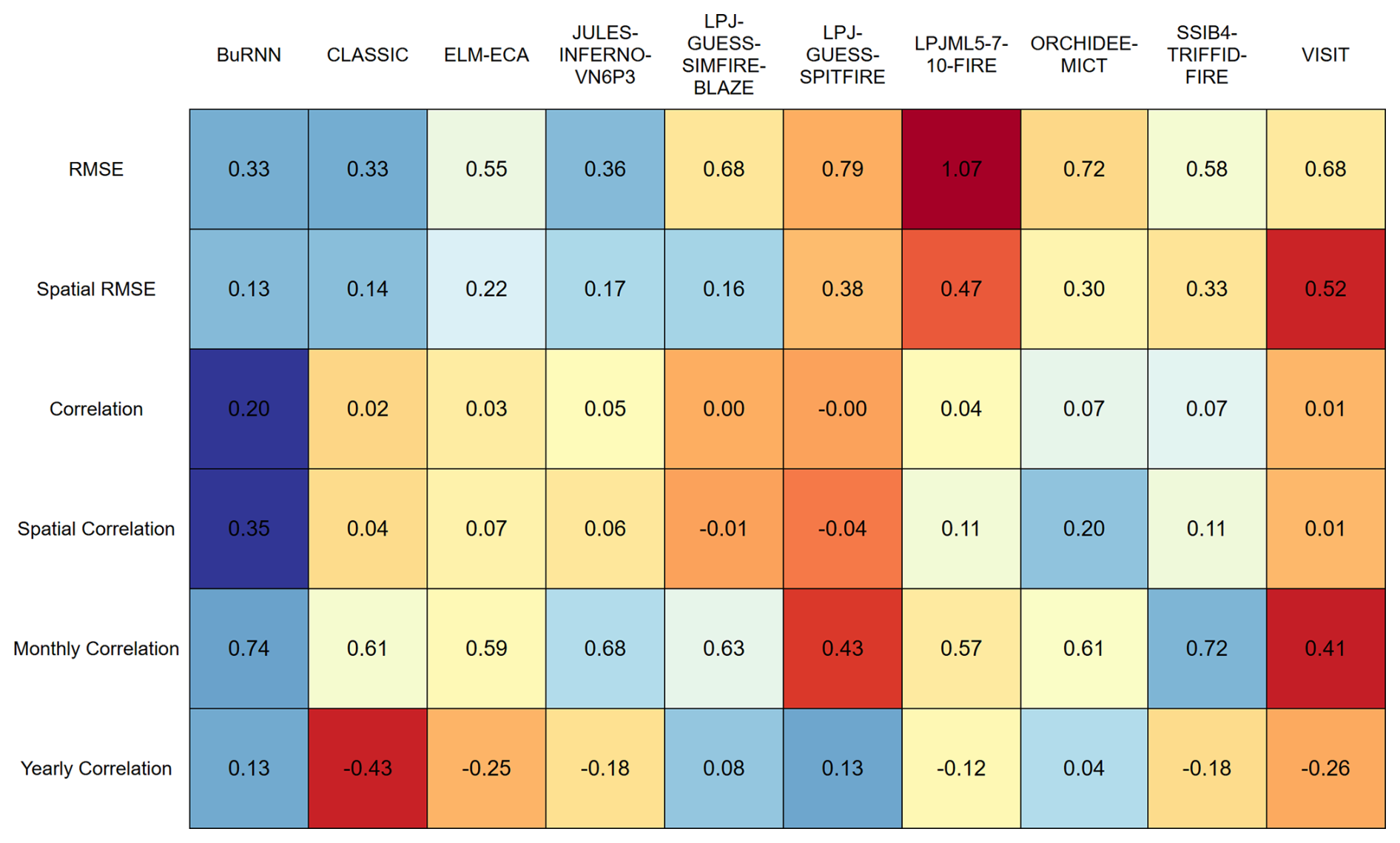
Figure A16 Evaluation scores of BuRNN and the FireMIP models in MIDE. Colour scaling is based on the normalized values with the minimum and maximum values set to −2 and 2 (σ). Better scores are marked in blue, while worse performance is in red.

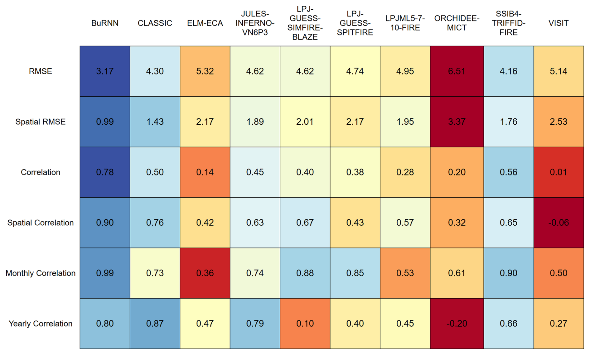
Figure A17 Evaluation scores of BuRNN and the FireMIP models in NHAF. Colour scaling is based on the normalized values with the minimum and maximum values set to −2 and 2 (σ). Better scores are marked in blue, while worse performance is in red.

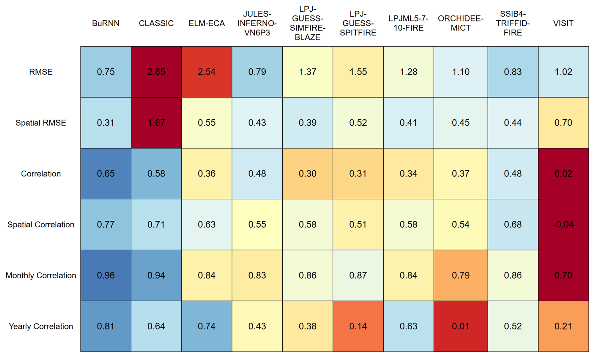
Figure A18 Evaluation scores of BuRNN and the FireMIP models in NHSA. Colour scaling is based on the normalized values with the minimum and maximum values set to −2 and 2 (σ). Better scores are marked in blue, while worse performance is in red.

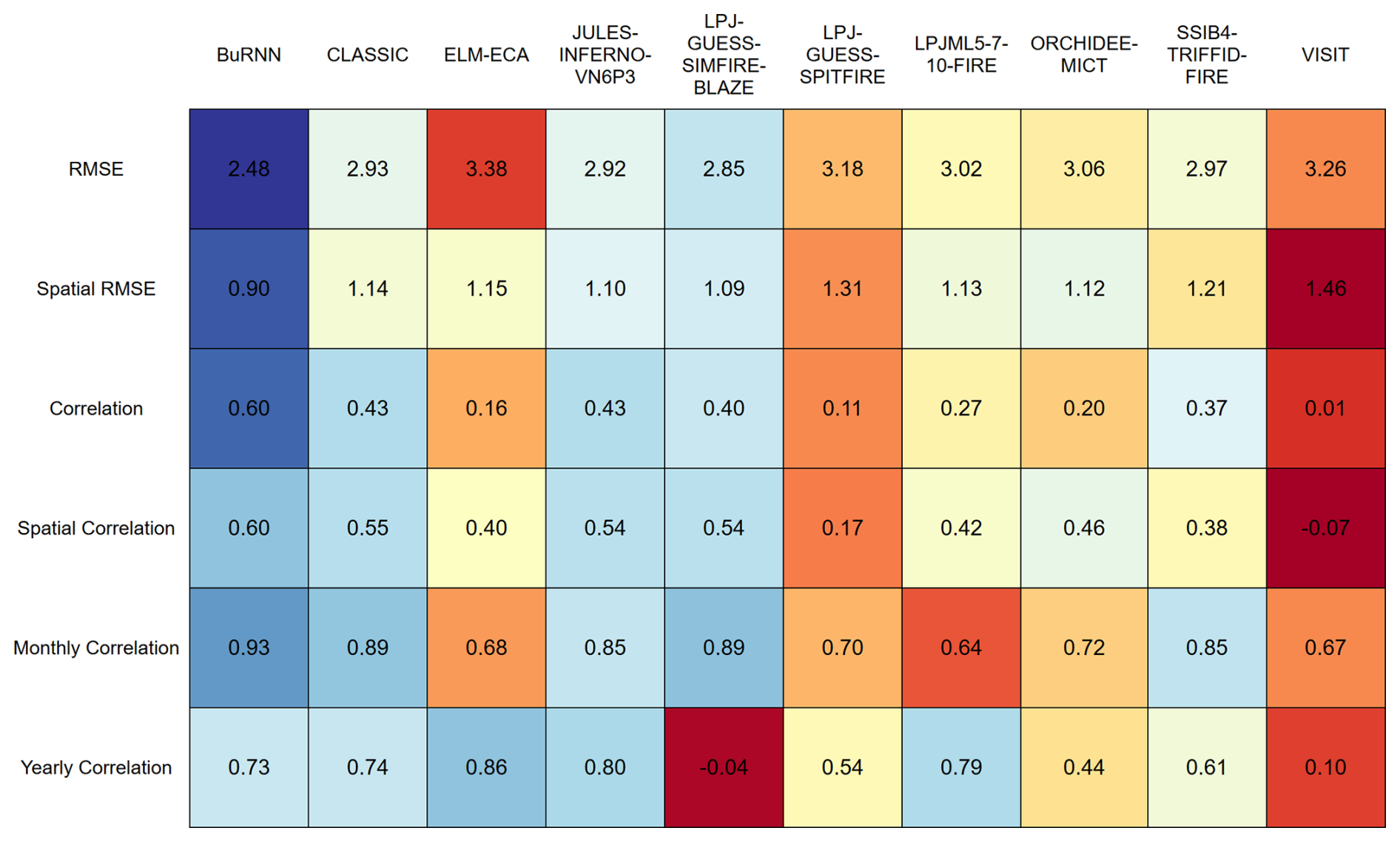
Figure A19 Evaluation scores of BuRNN and the FireMIP models in SEAS. Colour scaling is based on the normalized values with the minimum and maximum values set to −2 and 2 (σ). Better scores are marked in blue, while worse performance is in red.

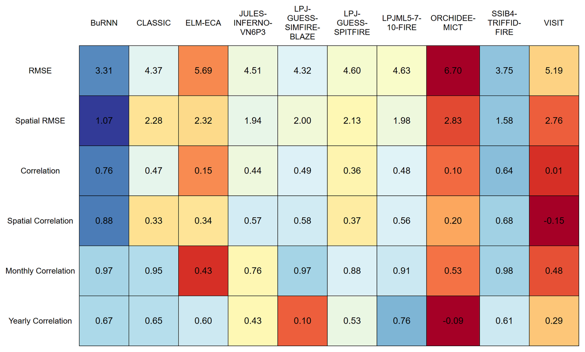
Figure A20 Evaluation scores of BuRNN and the FireMIP models in SHAF. Colour scaling is based on the normalized values with the minimum and maximum values set to −2 and 2 (σ). Better scores are marked in blue, while worse performance is in red.

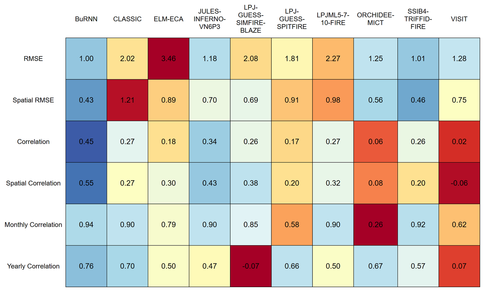
Figure A21 Evaluation scores of BuRNN and the FireMIP models in SHSA. Colour scaling is based on the normalized values with the minimum and maximum values set to −2 and 2 (σ). Better scores are marked in blue, while worse performance is in red.

Figure A22 Evaluation scores of BuRNN and the FireMIP models in TENA. Colour scaling is based on the normalized values with the minimum and maximum values set to −2 and 2 (σ). Better scores are marked in blue, while worse performance is in red.

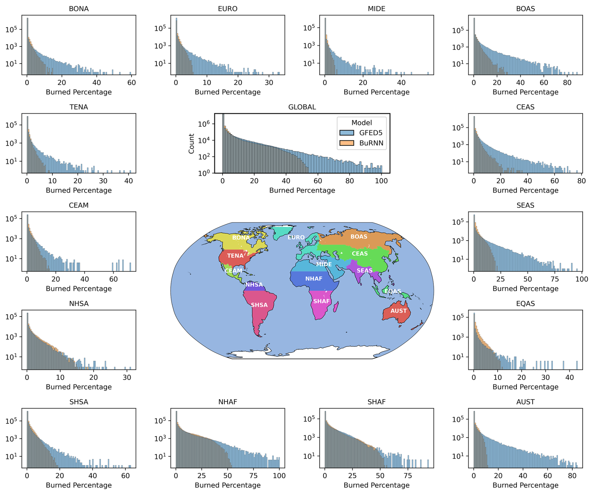
Figure A23 Histograms of the observed (blue) and modelled (orange) burned area (in % land surface area) for 1997–2019.

Table A1 Models used for the calculation of the ISIMIP Biome characteristics.

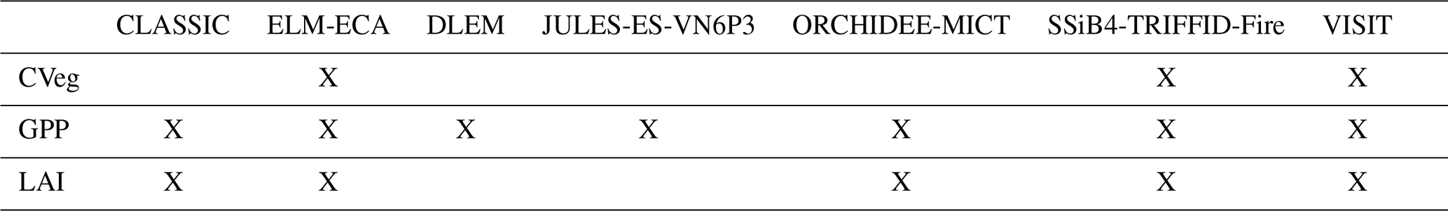
Table A2 Theil-Sen slopes of observed and modelled annual burned area for 2003–2019. The cells depict mean ±2 SD of annual burned area trend in Mha yr⁻¹.

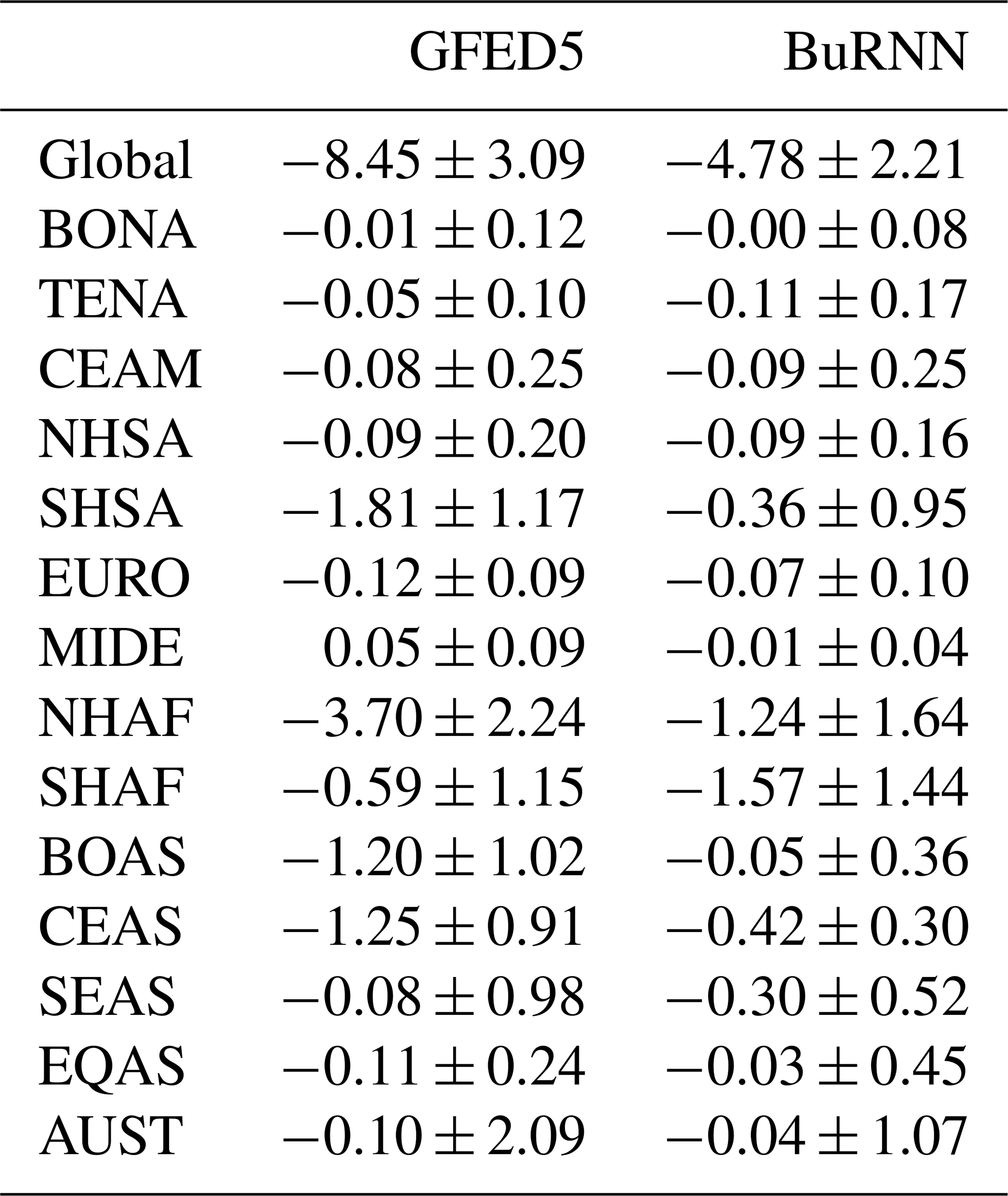
Table A3 Regional comparison of the observational products GFED5 and FireCCI51.

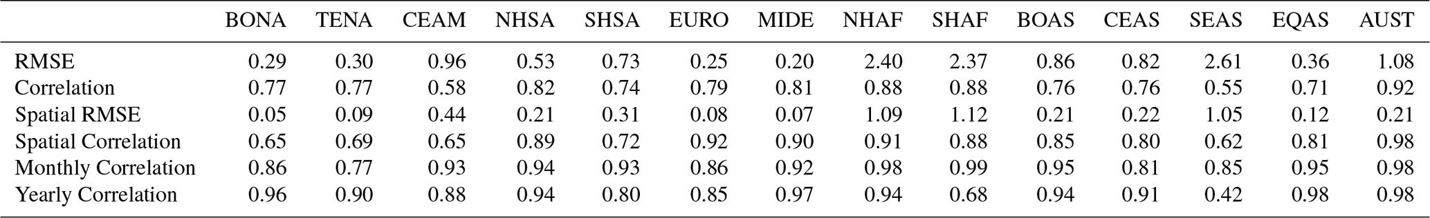
Table A4 Regional correlation of annual burned area of BuRNN and FireCCiLT11 (1982–1993 and 1997–2018) and between FireCCiLT11 and GFED5 (1997–2018).