Pysammos 1.0.0: a discrete-to-continuum transformation Python tool to analyse the rheology of granular materials

Granular flow processes involving different interstitial fluids and coupling regimes are widespread in both natural systems (e.g., landslides, rock avalanches, river sediment transport) and industrial applications (e.g., aggregates in concrete manufacturing, powder technology, animal feed). Despite this, the behaviour of complex granular flows is not fully understood. Modelling of granular media through software packages that couple the Discrete Element Method with Computational Fluid Dynamics (DEM-CFD) enables a comprehensive description of granular small-scale mechanics through simulations of particle-particle and particle-fluid interactions at high temporal and spatial resolution. These approaches are pivotal in the development of constitutive models that represent the bulk rheology of granular media. While DEM-CFD simulations provide particle-scale information (e.g., particle velocities and forces), extracting continuum fields requires a discrete-to-continuum (D2C) transformation that applies a mathematical approach termed coarse-graining. Although some DEM software packages include built-in D2C capabilities, others, such as MFiX-DEM, do not. Consequently, users are often required to develop custom D2C workflows or adapt simulation outputs to the requirements of other D2C tools. Hence, we introduce Pysammos, a Python package that performs discrete-to-continuum transformations and is designed to be user-friendly, open-source, and computationally efficient. Pysammos is able to process polydisperse granular mixtures of any particle shape, while also offering the option to analyse different particle phases separately. It post-processes output files from MFiX-DEM software and produces vtkhdf outputs ready for visualisation in ParaView, as well as a more generic h5 format for further data analysis. Pysammos is able to operate on standard desktop computers as well as on HPC systems. Finally, we showcase a variety of exemplar applications such as sediment erosion, crystals and magma in a conduit, bedload transport and impact cratering.

1 Introduction

Granular media on Earth are two-phase systems comprising a discrete solid phase (i.e., particles) and an interstitial fluid phase (e.g., air, water), in which the solid particles are in contact or near contact (Babic, 1997). Granular media are widespread in our everyday lives – from pharmaceutical pills, animal feed, cereals, snow, to blood cells suspended in plasma (Guazzelli, 2024). They are the second-most-handled material by weight in global industry only behind water (de Gennes, 1999) – e.g., aggregates in concrete manufacturing, mineral and powder processing, crushed oil shale and pebble bed nuclear reactors (Savage, 1984). They also govern the behaviour of a variety of highly hazardous natural flows – e.g., snow avalanches, debris flows, rock avalanches, landslides and dense pyroclastic density currents – and natural processes that interact with human systems – e.g., bedload transport in rivers and soil creep (Blatny et al., 2024; Garres-Díaz et al., 2020; Lucas et al., 2014; Lube et al., 2020). Hence, understanding granular media is essential for the resolution of numerous technological and scientific problems. However, the dynamic properties of granular media remain poorly constrained due to their wide-ranging nature (Kamrin et al., 2024).

1.1 The complexity of granular flows

The ongoing search for constitutive relations that unify the multifaceted behaviour of granular media is hindered by the breadth of complex characteristics and phenomenology of these materials. For instance, they encompass a wide distribution of particle sizes, shapes, roughnesses and elasticities, which control their macroscopic dynamic properties. Additionally, the spatial distribution of the properties of the granular medium may change throughout the course of the flow, due to granular segregation – where particles segregate by size, density, shape, and cohesive properties (Dai et al., 2025) – or particle breakage (Tong et al., 2022; Breard et al., 2023a).

Furthermore, they also exhibit a strong dependence on the characteristic length scale (i.e., particle size) (Koval et al., 2009). This implies that the role of the microscopic length scale may not vanish at the macroscopic continuum scale, that is, the particle size is of the same order of magnitude as the scale of spatial variation of macroscopic fields (Harper et al., 2025).

Granular flows also show evidence of recording deformation history, implying that a previous deformation episode predisposes the initial conditions of the material (Schofield and Wroth, 1968; Roux and Radjai, 1998). For instance, a high-shear episode to a granular packing with an initially isotropic contact network can induce dilation and preferentially align the force chains. This new fabric alters the initial state for any subsequent deformation, usually providing a higher shear strength relative to the initially isotropic packing.

The role of the interstitial fluid introduces an additional level of complexity in multiphase granular flows. What is more, the interplay between the solid and fluid phases changes between dilute and dense suspensions (Lube et al., 2020). The rheology is particularly challenging to capture in non-colloidal dense suspensions, as classical viscosity laws begin to break down due to the increase in energy dissipation through particle contacts (Gallier et al., 2014; Guazzelli, 2024).

These aspects of granular flows render their continuum representation particularly difficult. Nonetheless, since the surge of computers, modelling of discrete particle systems has been made possible through the Discrete Element Method (DEM). Despite its computational limitation to small scale systems, it is an invaluable tool for simulating complex granular flows without involving any continuum assumptions.

1.2 Using DEM to study granular flows

The DEM explicitly applies Newton’s second law of motion to the particle centres and the force displacement law at the contacts, to compute trajectories of individual granular particles from the forces exerted on particles, and vice versa, over time periods in which accelerations are assumed to be constant (Cundall and Strack, 1979). Collisions are assumed viscoelastic, conceptualised as a spring-dashpot system – whose components respectively represent the repulsive force and the dissipated kinetic energy – although other contact models have also been implemented (Dobry and Ng, 1992).

DEM was first developed by Cundall (1971) for a rock mechanics application and was later extended by Cundall and Strack (1979) for applications in granular media. Later it began to be applied to molecular dynamics (Walton, 1980), and soil mechanics (Rothenburg and Bathurst, 1989). Coupling of DEM with Computational Fluid Dynamics (CFD) began in the early 1990s with Tsuji et al. (1993), widening the range of applications of DEM to the study of multiphase granular flows.

In recent decades, DEM has become a powerful tool to study numerous natural processes in the field of geosciences: seismic wave propagation in unconsolidated sediments (O'Donovan et al., 2016); impact cratering on granular asteroids (Sánchez et al., 2022); emplacement of igneous intrusions (Morand et al., 2024); magma mush dynamics (Carrara et al., 2024); erosion processes (Breard et al., 2022); bedload transport (Alihosseini et al., 2020); probing granular flow rheology from the basal force function (Zrelak et al., 2024, 2026), and thermal-geomechanical coupling effects in geothermal reservoirs (Baghban et al., 2021), amongst others.

1.3 The transition from discrete to continuum

An essential service of DEM is that of providing the accurate particle dynamics from which we can obtain macroscopic quantities relevant for continuum-mechanical and/or statistical-mechanical formulations of those systems. The gap between discrete particle data and macroscopic fields may be bridged through discrete-to-continuum (Discrete2Continuum, D2C) transformations, which apply coarse-graining (CG) methods to DEM data to derive bulk quantities (e.g., stress tensor) projected onto continuum macroscopic fields. CG methods are grounded on the principle that macroscopic fields emerge as averages of microscopic quantities. It is worth noting this use of coarse-graining is distinct from coarse-grained DEM, a computational technique in which large populations of small particles are represented by fewer larger surrogate particles (e.g., Kishida et al., 2025). Hereafter, the term “coarse-graining” will be used specifically to refer to the mathematical methods in D2C transformations.

Several CG formulations have been developed over the years. Early formulations were restricted to the quasi-static regime – whereby the inertial terms were neglected in the microscopic balance equations (Christoffersen et al., 1981) – or to the rapid flow regime – assuming only binary particle collisions (Jenkins and Savage, 1983). Some of these procedures are still used today to post-process DEM models that represent static systems (e.g., the host rock of a magma intrusion, Morand et al., 2024). Later, formulations began to include inertial terms (Walton and Braun, 1986; Zhang and Campbell, 1992), although with incomplete derivations, as Babic (1997) corroborates.

However, the earlier averages were carried out within discrete or hard spatial boundaries – i.e., non-differentiable, hence inadequate for the derivation of macroscopic (differential) balance equations. It is not until Babic (1997), that a general averaging approach across granular flow regimes, suitable to obtain average balance equations for multiphase granular media, is introduced in the literature. The principles used by Babic (1997) seem to be an adaptation of the almost coetaneous comprehensive derivation of continuum balance equations through spatio-temporal weighted averages in the field of molecular dynamics by Murdoch and Bedeaux (1994).

Ever since Babic (1997), CG theory has been honed to simplify the derivations therein (Glasser and Goldhirsch, 2001), to be valid near to hard boundaries (Weinhart et al., 2012), to address averaging scale dependency (Artoni and Richard, 2015), to discuss appropriate spatial averaging resolution (Weinhart et al., 2013), to study the contribution of individual particle phases in polydisperse systems (Tunuguntla et al., 2014), and to account for contacts between particles of irregular shape (Weinhart et al., 2016).

Other CG methods exist in the literature, such as binning or the method of planes, however, they lack key advantages of the spatial weighted average. With the CG that performs a spatial weighted average: the macroscopic fields satisfy the average balance of continuum mechanics equations; the fields can be evaluated at every point in space; and particles are not assumed to be spherical or rigid (Tunuguntla et al., 2017).

1.4 Available discrete-to-continuum tools

Nowadays, there are numerous DEM code packages, both open-source – e.g., LAMMPS (Plimpton, 1995), LIGGGHTS (Kloss et al., 2012), YADE (Smilauer et al., 2015), MercuryDPM (Weinhart et al., 2020a), MFiX (Syamlal et al., 1993) – and closed-source or commercial codes – e.g., Altair EDEM (Siemens) (Altair Engineering, Inc., 2025), PFC (Itasca Consulting Group, 2025), and Iota-Suite (although no longer operational) (Morrissey et al., 2020). Regarding open-source software, some offer an inbuilt D2C transformation, that is the case of LAMMPS, with a standard volume averaging, and MercuryDPM, with a weighted average in their MercuryCG. Others, like MFiX do not provide that post-processing step, which leads users to build their own D2C code or adapt their DEM software outputs to the format other inbuilt D2C software require. Some of the closed-source software, such as Altair EDEM, also provide their own continuum analysis tools.

1.5 An overview of Pysammos

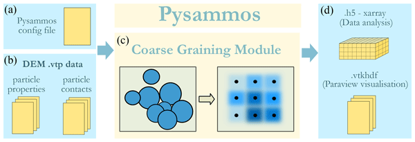
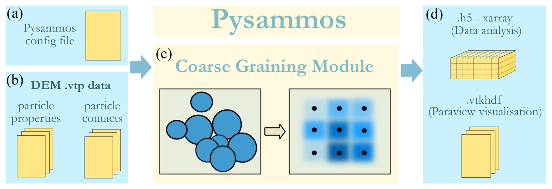
The purpose of this work was to build Pysammos, a Python package designed with the aim of providing a user-friendly D2C workflow to post-process data from the MFiX open-source DEM software, and provide a streamlined visualisation in widely used open-source visualisation software, ParaView (Fig. 1). This code package provides flexibility in the output variable selection, mesh parametrisation, and data analysis of the obtained results. The efficient algorithmic complexity exhibited by Pysammos avoids the requirement of extensive computational resources, making it a program that can be run at the same time as other processes. Its modular design enhances DEM analysis across users with varying expertise, as it does not require access to inner-level source code. This is intended to encourage a broader use of DEM in geoscientific research, where many observed processes involving discrete elements are currently modelled as a continuum but could benefit from a discrete insight.

Figure 1 Conceptual diagram of the code's main functionality (c), types of input (a, b), and output (d). For further details on output structure and code architecture, see Fig. 3. Appendix A contains additional information on the configuration file and the specific DEM data required.

The name of the package is a reference to a work by Archimedes called The Sand (Greek: psammos) Reckoner, in which he endeavoured to determine the number of grains of sand that could fit in the universe (Archimedes, 2009). To do so, he created a new system of large number notation, given that the number system at that time could only express values up to a myriad (10 000). Similarly, Pysammos is concerned with the efficient handling and analysis of a large number of DEM particles. The name of the package thus reflects the shared focus on managing vast quantities of discrete elements, from grains of sand to simulated particles.

Below we present the coarse-graining mathematical theory implemented in Pysammos; a description of the code workflow, methodologies and features; and a presentation of its performance, benchmarking against other CG codes, and a showcase of examples relevant to the geoscientific community.

2 Theory of coarse-graining

In this section we review the theory of coarse-graining as a spatial weighted average, and the caveats involved in the calculation of some continuum fields. We also discuss the implications of time-averaging and the importance of a suitable smoothing width. Finally, we introduce the framework to calculate the partial contribution of various species within a particulate mixture.

2.1 A weighted spatial average

In this work, we refer to coarse-graining as a generalised weighted averaging approach to compute macroscopic continuum fields from microscopic discrete quantities (e.g., DEM observables: particle velocity and forces), such that they satisfy the average balance of equations for granular media. The contribution of each particle to the macroscopic field evaluated at any given point is weighted according to the relative position of the particle's centre of mass to the point. CG is applicable to a range of flow regimes – from the solid-like quasi-static mode, to the fluid-like rapid flow mode, for granular media of arbitrary particle size, shape and rigidity (Babic, 1997). The collisions are assumed not to be instantaneous.

Coarse-graining conceptualises an assembly of discrete solid particles as a system of discrete mass points located at the particle centres, as per the principles of statistical mechanics (Babic, 1997). Hence, the microscopic discrete mass density field (ρ^discrete) at a point in space (r) and time (t) is given by the convolution of the mass (m_i) of particle i (located at r_i) and the Dirac delta function (δ), as shown in Eq. (1) (Glasser and Goldhirsch, 2001). Note that δ is zero everywhere except at the particle centres, where it is infinitely high, and has a total integral of one.

$$\begin{array}{}\text{(1)}& {\mathit{\rho }}^{\mathrm{discrete}}(\mathit{r},t)=\sum _{i=\mathrm{1}}^N{m}_i\mathit{\delta }(\mathit{r}-{\mathit{r}}_i(t\left)\right)\end{array}$$

Similarly, the macroscopic continuum mass density field is obtained by convolving the particle mass with a coarse-graining function, Ψ, as described in Eq. (2) (Weinhart et al., 2012).

$$\begin{array}{}\text{(2)}& \mathit{\rho }(\mathit{r},t)=\sum _{i=\mathrm{1}}^N{m}_i\mathrm{\Psi }(\mathit{r}-{\mathit{r}}_i(t\left)\right)\end{array}$$

The net effect of Ψ is the smearing of the Dirac delta function of Eq. (1) across a volume of radius c and effective smoothing width w (see Sect. 3.5.3). Hence, Ψ has dimensions of inverse volume, and the sum of the weights across that volume is 1 (Eq. 3) (Babic, 1997).

$$\begin{array}{}\text{(3)}& \underset{{\mathbb{R}}^{\mathrm{D}}}{\int }\mathrm{\Psi }\left(\mathit{r}\right)\mathrm{d}\mathit{r}=\mathrm{1}\end{array}$$

Hence, by performing a spatial weighted average, the contribution of several particles is taken into account in the evaluation of a macroscopic continuum field at a given point in space. In order for the macroscopic fields to satisfy the continuum balance of equations, they must be smooth across space. This requires the coarse-graining function Ψ to be differentiable everywhere. Several weighting functions are commonly seen in the literature: the Lucy polynomial function (Lucy, 1977), the Heaviside step function, and the cut-off Gaussian function (see Sect. 3.5.3).

2.2 Averaging the interaction between particles

Continuum fields that correspond to a quantity representing the interaction between two particles are evaluated differently: by distributing the field along the branch vector connecting the two particles (Babic, 1997). The stress tensor is defined as the sum of the contact stress tensor (σ^c) and the kinetic stress tensor (σ^k), as shown in Eq. (4) (Babic, 1997).

$$\begin{array}{}\text{(4)}& \mathit{\sigma }(\mathit{r},t)={\mathit{\sigma }}^c(\mathit{r},t)+{\mathit{\sigma }}^k(\mathit{r},t)\end{array}$$

The contact stress tensor is defined in Eq. (5).

$$\begin{array}{}\text{(5)}& {\mathit{\sigma }}^c(\mathit{r},t)=\sum _{i=\mathrm{1}}^N\sum _{j=i+\mathrm{1}}^N\sum _{k=\mathrm{1}}^{C_{ij}}{\mathit{f}}_{ij}^k\otimes {\mathit{a}}_{ij}^k\underset{\mathrm{0}}{\overset{\mathrm{1}}{\int }}\mathrm{\Psi }(\mathit{r}-{\mathit{r}}_i+s{\mathit{a}}_{ij}^k)\mathrm{d}s,\end{array}$$

where N is the number of particles in the system, and C_ij is the maximum number of contact points between two particles. The force between the particles i and j at the kth contact point is represented as ${\mathit{f}}_{ij}^k$. The branch vector ${\mathit{a}}_{ij}^k$ is defined as the distance between the kth contact point and the centre of particle i. The dummy variable s parametrises the line segment from particle i to a contact point. The integral of the CG function Ψ over the projection of s on ${\mathit{a}}_{ij}^k$, enables the contact force to be spatially distributed along the branch vector, ensuring a smooth representation of the contact stress (Fig. 2). Note that Eq. (5) does not account for wall-particle interactions; this extension is discussed in detail in Weinhart et al. (2012).

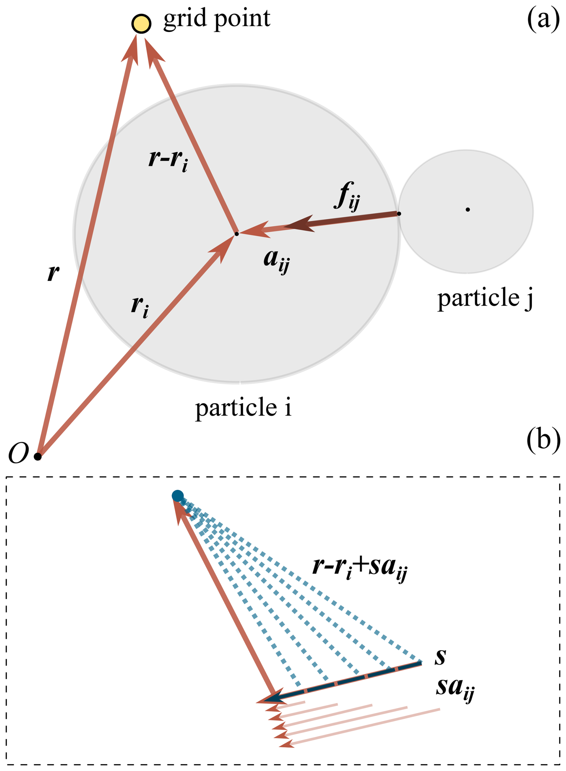
Figure 2 Vectors involved in the calculation of the contact stress tensor over one particle. In panel (a), r and r_i represent the positions of the grid point (yellow) at which the coarse-grained fields are evaluated, and the centre of mass of particle i (black), respectively. The branch vector a_ij, connects r_i and the contact point between the two particles. The displacement vector from particle i and the grid point is denoted by r−r_i. The force acting on particle i resulting from the collision with particle j, f_ij, is represented by the brown vector. Panel (b) illustrates the integration of the weighting function Ψ (evaluated at r−r_i) along a stepwise projection of a_ij (Eq. 5). The scalar s parametrises the line segment corresponding to a_ij. Hence, the integral of Ψ over its projection onto a_ij spatially distributes the collisional force along the branch vector, providing a smooth representation of the contact stress.

2.3 The influence of velocity gradients

The coarse-grained velocity field may be distinguished from individual particle velocities, which generally exhibit higher velocities than the macroscopic field. The difference between these two velocities is referred to as the fluctuation velocity of the particle. To prevent it from vanishing to zero, it is represented by its magnitude (Goldhirsch, 2008).

The kinetic stress tensor, calculated with the fluctuation velocity (Eq. 6), has been shown to depend on averaging width (Glasser and Goldhirsch, 2001; Artoni and Richard, 2015; Weinhart et al., 2016).

$$\begin{array}{}\text{(6)}& {\mathit{\sigma }}^k(\mathit{r},t)=\sum _{i=\mathrm{1}}^N{m}_i{\mathit{V}}_i^{\prime }{\mathit{V}}_i^{\prime }\mathrm{\Psi }(\mathit{r}-{\mathit{r}}_i(t\left)\right),\end{array}$$

The scale dependency arises from the fact that in Eq. (6) the fluctuation velocity, ${\mathit{V}}_i^{\prime }$ (Eq. 7), is defined with respect to the field velocity at r, V(r,t), and not at the position of the particle's centre of mass, r_i, i.e. V(r_i(t),t), in order to satisfy the continuum balance of equations at r (Glasser and Goldhirsch, 2001). Nevertheless, ${\mathit{V}}_i^{\prime }$ can be decomposed into two terms in order to isolate the scale dependency of σ^k, as shown below.

$$\begin{array}{}\text{(7)}& \begin{array}{rl}{\displaystyle }{\mathit{V}}_i^{\prime }& {\displaystyle }={\mathit{v}}_i\left(t\right)-\mathit{V}(\mathit{r},t)\\ {\displaystyle }& {\displaystyle }={\mathit{v}}_i\left(t\right)-\mathit{V}\left({\mathit{r}}_i\right(t),t)+\mathit{V}\left({\mathit{r}}_i\right(t),t)-\mathit{V}\left(\mathit{r}\right(t),t)\\ {\displaystyle }& {\displaystyle }={\mathit{V}}_i^{*}+\mathit{V}\left({\mathit{r}}_i\right(t),t)-\mathit{V}\left(\mathit{r}\right(t),t),\end{array}\end{array}$$

where v_i(t) is the velocity of the ith particle at time t, and ${\mathit{V}}_i^{*}$ is the fluctuation velocity field evaluated at the particle's centre of mass, r_i(t). The latter terms of ${\mathit{V}}_i^{\prime }$ capture the scale dependency due to velocity gradients. In the absence of these gradients, the scale dependency vanishes, and the fluctuation velocity simplifies to ${\mathit{V}}_i^{\prime }={\mathit{V}}_i^{*}$. Alternatively, Weinhart et al. (2013) propose an a posteriori correction to obtain the scale-independent term of the kinetic tensor, thus bypassing the evaluation of the fluctuation velocity at r_i by means of interpolation.

Nonetheless, the granular temperature is a measure that focuses solely on the local particle fluctuations, at r_i. Hence, only the scale-independent part of σ^k is used to compute granular temperature (Eq. C13 in Appendix C2).

2.4 Time averaging

Traditional statistical mechanics considers multiple realisations, or probabilistic copies of a system, over which the corresponding macroscopic quantities are averaged (Jaynes, 1957). This conceptual tool is equivalent to averaging over the total time range, an equivalence classically derived for ergodic systems in equilibrium (Huang, 1987), but which extends to systems at (non-equilibrium) steady state, where the relevant statistics are stationary in time (Babic, 1997). This is advantageous for systems that are complex to simulate over large time scales. In the case of granular media we are able to simulate complex granular systems for longer time scales with DEM. Hence, in the field of computational granular physics, ensemble averaging is not required (Glasser and Goldhirsch, 2001), and in fact could be problematic due to the inherent lack of scale separation. Instead, the analytical expressions for continuum fields tend to include a time-averaging, as well as a space-averaging, which acts as a low-pass filter on the inherent fluctuations of granular flows, to obtain steady-state solutions (Babic, 1997; Glasser and Goldhirsch, 2001). Nevertheless, the time averaging is not strictly required, and in fact, even moving window Heaviside temporal averages could obscure time-dependent trends in highly transient flows, as pointed out by Weinhart et al. (2012). Hence, in this study only spatial averaging is considered for the analytical equations of coarse-graining.

2.5 Smoothing width

The choice of averaging width w, i.e., the resolution of the continuum fields resulting from CG, has been shown to be non-trivial. Babic (1997) proposes that the averaging should be computed over a representative volume, which is a region where no gradients occur, calling this the “continuum assumption”. In particular, the macroscopic kinetic tensor field has been shown to intrinsically depend on the square of the smoothing width (Glasser and Goldhirsch, 2001). Weinhart et al. (2013) find two apparent CG length scales for which the coarse-grained macroscopic fields are almost independent of the averaging width: one at sub-particle scale, which is able to resolve flow layers close to the lower boundary of the modelled inclined flow, and one at particle scale, which yields smooth continuum fields.

2.6 Mixture theory

To evaluate the partial contribution of various species, or phases, within a particulate mixture, we make use of mixture theory. It conceptualises the granular mixture to be simultaneously populated by all phases, with associated partial macroscopic fields (Tunuguntla et al., 2017). The macroscopic fields of the mixture are hence obtained by superposing (i.e., summing) the partial fields (Eq. 8).

$$\begin{array}{}\text{(8)}& \mathcal{F}=\sum _{\mathit{\nu }}{\mathcal{F}}^{\mathit{\nu }}\end{array}$$

A phase can be defined as any particle property, or combination of such, that contributes to particle segregation, that is, density, size, shape, elasticity, roughness (Tunuguntla et al., 2017).

3 Methodology: code structure and algorithm steps

This section firstly describes how the architecture has been designed to facilitate maintenance, and to cater for the performance considerations inherent to DEM data processing. Subsequently, it provides a description of the input DEM data, and an overview of the algorithm steps of the CG workflow embedded and handled from the user-facing class.

3.1 Software design

The architecture of Pysammos is designed to be modular, dividing cumbersome code into smaller manageable tasks, to enhance readability, and to allow reusability and easy maintenance. Code modularisation in Python takes on the form of packages, modules and functions, thus building a hierarchical structure of code (Fig. 3). This is further aided by a hybrid implementation, combining object oriented programming (OOP) and functional programming (FP) approaches to optimise readability and maintainability. OOP provides a clear structural interface for encapsulating underlying computations, while FP is suitable for small reusable operations within or alongside OOP. The core code makes use of widely used scientific Python packages, such as NumPy (Harris et al., 2020), SciPy (Virtanen et al., 2020), VTK (Schroeder et al., 2006; Quammen, 2015), XArray (Hoyer and Hamman, 2017) and Numba (Lam et al., 2015).

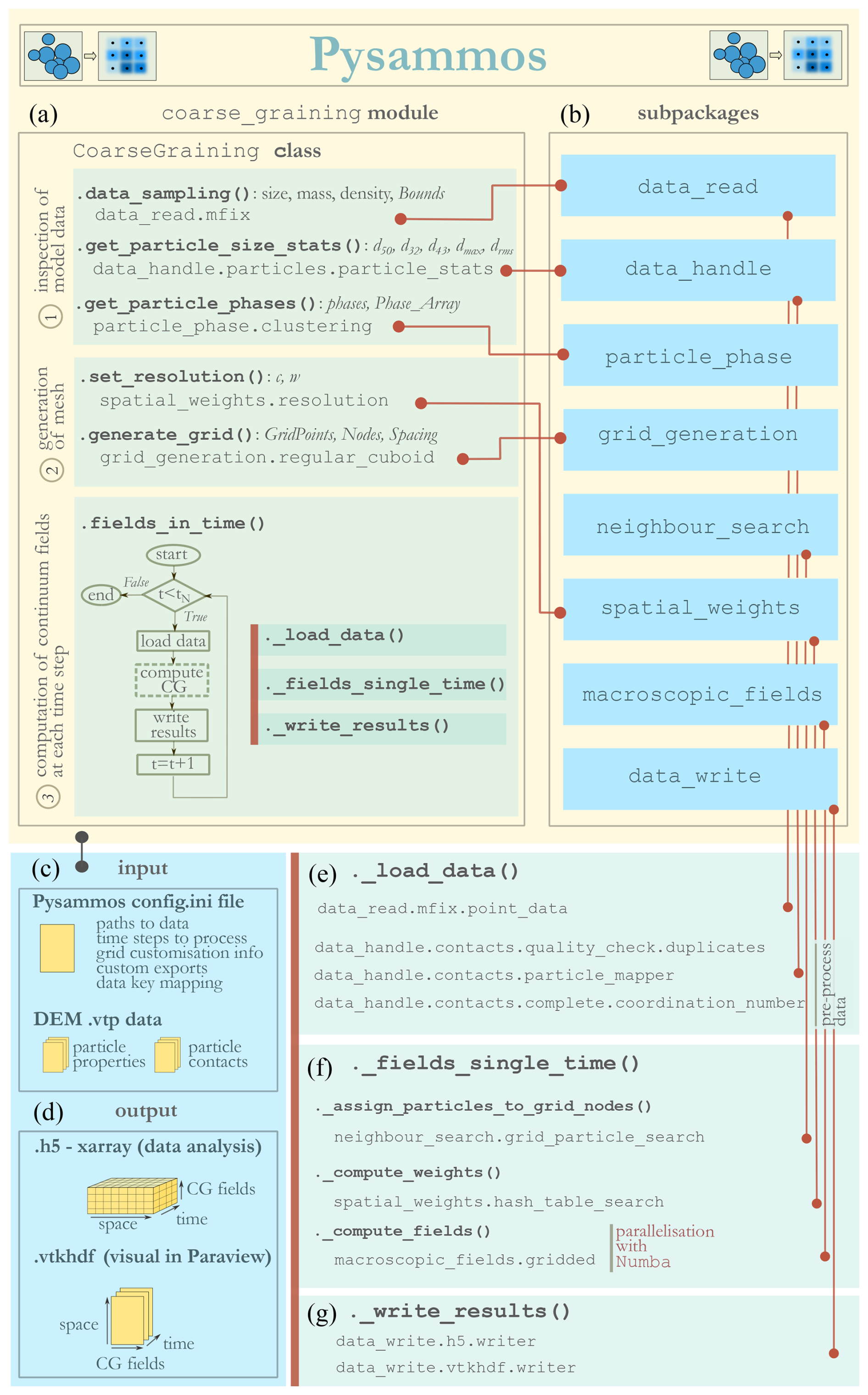
Figure 3 Conceptual schematic of the code architecture of the user-interface class CoarseGraining, defined in the main Pysammos module coarse_graining (a). The diagram illustrates the workflow structure of the class (green panels 1–3) and links each step to the corresponding source code in the relevant sub-packages (b) via red lines. Bold monospace text denotes class functions, while non-bold monospace text indicates the fully qualified module paths executed by each function. Function outputs and stored attributes are shown in normal and italic text, respectively. Panel 3 presents the computation of continuum fields across time steps as a flowchart, with each step corresponding to a hidden class method and further detailed in panels (e)–(g). The format and purpose of inputs and outputs are shown in panels (c) and (d).

3.1.1 User-facing class

The CoarseGraining class acts as the user-facing interface. The steps of the coarse-graining workflow correspond to the different class methods, which in turn orchestrate lower-level functions. Methods of the user-facing class may be grouped into three categories according to the CG workflow: (1) inspection of model data, (2) generation of continuum mesh, (3) computation of continuum fields at each time step (Fig. 3a). The class builds up its internal state sequentially, as task-oriented methods are called successively in the correct order, accumulating attributes in a pipeline style which subsequent methods rely on. While reducing boilerplate code, the sequential format suits the inherent progressive logic of the CG workflow, allowing a straightforward, readable and flexible interface flow for the user. Dependency fault tolerance, especially in the user interface class attributes, is implemented by checking that those attributes are stored as instance attributes before executing a method with dependencies (IEEE, 1990). The inputs to this class, provided in the configuration file (Appendix A), are stored as instance attributes and can be accessed throughout the lifetime of the object.

3.1.2 Performance optimisation

In addition to ensuring readability and maintainability, the structural design described above was driven by performance considerations inherent to DEM data processing. Typical DEM simulations may consist of 10⁴–10⁶ particles and 10²–10³ time steps, but it is not uncommon to have >10⁴ time steps in long duration high data save frequency simulations with a low number of particles. The computational cost of the code is dominated by data handling rather than individual numerical operations. The scalability of the execution gives rise to bottlenecks that limit efficiency due to memory bandwidth rather than raw CPU performance. Code performance was thus enhanced by tackling bottlenecks identified in the resource usage analysis, employing algorithmic optimisation or the Numba Python compiler. Each bottleneck was addressed with a unique strategy that suited that particular operation (Appendix E).

3.1.3 User profiles

The modularity of the code's architecture suitably separates code levels linked to different user profiles. The standard user only employs the user-facing class, modifying the inputs in the configuration file, and analyses data as suggested in the documentation examples. The advanced user might make changes to variables of the user-facing class that have been set to a specific value by default, and analyse the data differently for a more specialised application. The developer user makes modifications to low-level functions in the sub-packages, and is provided with benchmarked examples to ensure consistency and robustness in future developments required to keep Pysammos relevant in the DEM community. The principal communication channel for the developer users is intended to be GitHub, as it facilitates tracking code issues and development of new implementations. It also provides a space where any type of user can open discussions about code development suggestions or experiences with code issues via GitHub's issue tracker.

Below, we introduce the principal steps of the coarse-graining workflow as implemented in the CoarseGraining class. Each subsection corresponds to a major stage of the algorithmic pipeline presented in Fig. 3, highlighting both the functional role of each step, and the considerations associated with the design and performance of the code.

3.2 Input DEM data

The paths to the DEM data files and the corresponding variable names are supplied by the user either through the configuration file (Appendix A), or directly to the user-facing CoarseGraining class.

The input DEM data required for Pysammos consist of particle data and contact data, which are stored in separate files. The particle data include particle position, particle ID, velocity, diameter (or radius), density, volume, mass, and optionally coordination number. The contact data include the particle IDs of the two particles involved in each recorded contact, the force acting on the first particle, and the contact point position. If contact point positions are unavailable (e.g., when using earlier MFiX releases), Pysammos can recalculate them for spherical particles.

MFiX records single-sided contacts, providing the force vector acting on the first particle, and the contact point position. Since the contact point position is explicitly available, reconstruction of the full bidirectional contact list is valid regardless of particle size distribution – the branch vectors (a_ij in Eq. 5) are computed directly from particle centre positions and the contact point, rather than being inferred from particle geometry. The reconstruction procedure is described in Sect. 3.5.1 and the Appendices referenced therein.

3.3 Data inspection stage

The data inspection consists of obtaining relevant information on the provided DEM data that will be used later on in the program to apply safety checks or perform calculations (Fig. 3a, panel 1). Likewise, it also provides the user with a particle-size overview. It starts with the .data_sampling() method, which loads and inspects the particle data at the first time step that the user has chosen to process, thus obtaining arrays of particle diameter, mass, density and the bounds of particle positions – i.e., the extent of the model to be post-processed at the first chosen time step. These particle data are analysed in .get_particle_size_statistics() to get the median, root-mean-squared and maximum size, and area- and volume-weighted average particle size or diameter.

3.3.1 Phase detection algorithm

The DEM data are also analysed in .get_particle_phases() with the purpose of classifying the particles into phases, should the user require macroscopic fields of each particle phase. Here, a phase is defined by particle diameter and density (Fig. 4a, b), since they are two properties related to the two main competing mechanisms in segregation: kinetic sieving and buoyancy (Drahun and Bridgwater, 1983; Tripathi and Khakhar, 2013). Phase detection is fully automated in the current version (1.0.0); the user does not specify phase definitions or characteristics. In Pysammos the phase detection is carried out by clustering particle data using the k-means algorithm, explained in detail in Appendix B1. The optimum number of clusters is chosen to be that with the absolute maximum in silhouette value, a measure for how well each point matches its assigned cluster relative to the nearest neighbouring cluster (Appendix B1), as shown in Fig. 4e. Afterwards, the k-means algorithm is applied to the dataset with the optimum number of clusters (Fig. 4d) to obtain the phase-ascribed arrays, which are stored as attributes of the class instance.

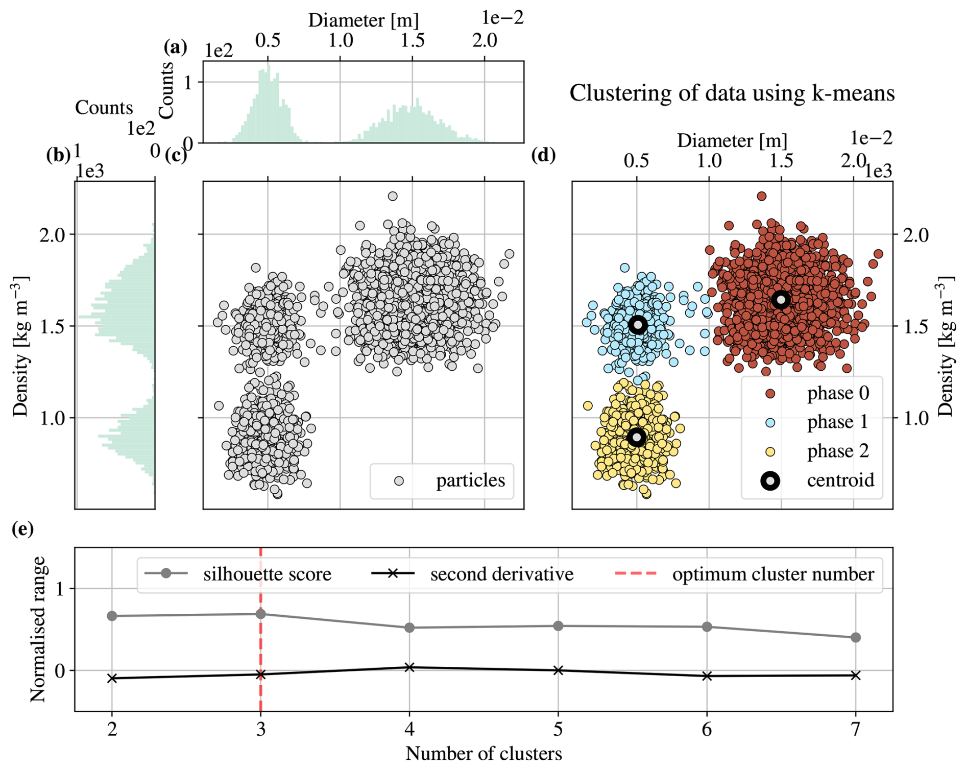
Figure 4 Illustration of the approach to detect particle phases. Synthetic data set of a bimodal particle diameter distribution (a). Synthetic data set of a bimodal particle density distribution (b). Cross-plot corresponding to the diameter and density distributions in (a) and (b), respectively (c). Cross-plot containing the same particle samples as (c) coloured by the phase they are classified to according to the k-means algorithm using the optimum number of clusters (d). Silhouette score for a given number of clusters employed in the k-means algorithm (grey), and the corresponding second derivative (black) (e). The absolute maximum in (e) is chosen to be the optimum number of clusters (dashed red).

3.4 Mesh generation stage

The mesh is created with a resolution w (Eq. 9) specified in .set_resolution(). It is calculated as $w=m_w\overline{d}$, where m_w is a scaling and $\overline{d}$ is a representative particle size. By default, m_w is 0.75 (Weinhart et al., 2016). In polydisperse granular media the choice of $\overline{d}$ is not trivial (Polanía et al., 2025), hence, we provide different metrics for the user to choose from, such as the median diameter or d₅₀, the root mean squared diameter (d_rms), volume-weighted average (d₄₃) and area-weighted average or Sauter diameter (d₃₂).

The mesh domain can be user-defined or automatically determined from the model bounds. In the latter case, the mesh spans the extent of the model while leaving a safety margin to the boundaries proportional to the maximum grain size and averaging scale. In the case of 1D or 2D automatically generated meshes, the domain is reduced along one direction by taking a central transect perpendicular to that dimension.

The method .generate_grid() generates a structured grid with the specified spacing. Currently only a simple regular cuboid grid is available. Nevertheless, the code structure allows the additional implementation of new mesh types. Note that in this work, mesh refers to a general discretisation of space, while grid refers to the current structured Cartesian implementation.

3.5 Coarse-graining stage

The calculation of continuum fields across all time steps is encapsulated in .fields_in_time(). It makes use of hidden methods of the class, prefixed with an underscore, to organise internal logic and condense recurring functionality. For each time step processed, the data are loaded, the continuum fields are calculated, and output files are written (Fig. 3e–g). The field evaluation is broken down into particle and grid point association, weight computation, and the computation of the different fields (Fig. 3f).

3.5.1 Data reading and handling

The particle and contact data described in Sect. 3.2 are retrieved from the MFiX .vtp file using the variable names specified in the configuration file (Appendix A).

Regarding contact data, Pysammos reconstructs the full bidirectional contact list by duplicating each particle pair, applying the opposite force to the second particle, and assigning the same contact point to both entries. For concave particles, multiple contact points between the same particle pair are explicitly reported and are handled as distinct contacts in our analysis. For convex particles, in contrast, the contact is represented by a single point at the centre of the overlapping volume.

Several data mapping structures and algorithms are used in the pre-processing stage prior to applying CG. Following the data ingestion, DEM data are sorted by particle ID, facilitating the mapping of contact data onto the global particle data (Appendix D1), so that branch vectors between particle pairs can be computed. Subsequently, pre-processing steps are applied to ensure data quality, including the identification and removal of duplicated contacts written during parallel execution (Appendix D3). During branch vector computation, periodic boundaries are accounted for by evaluating displacements to the nearest periodic equivalent (Appendix D2).

3.5.2 Particle search

Continuum macroscopic fields consist of the spatial weighted average of microscopic particle quantities within a finite volume around any point in space (Fig. 5). The particles within this volume are identified based on the distances between particle centres and grid points, using a k-d tree–based nearest-neighbour search, which efficiently identifies, for all grid points in a single query, the particle centres within a cut-off distance of each point (Appendix B2). The code subsequently organises this information into a compact array-based format optimised for performance and robustness (Appendix D4). To improve computational efficiency, the search is performed only once every time step, and the resulting neighbour information is employed in all subsequent calculations of fields involving either individual particles or interparticle interactions.

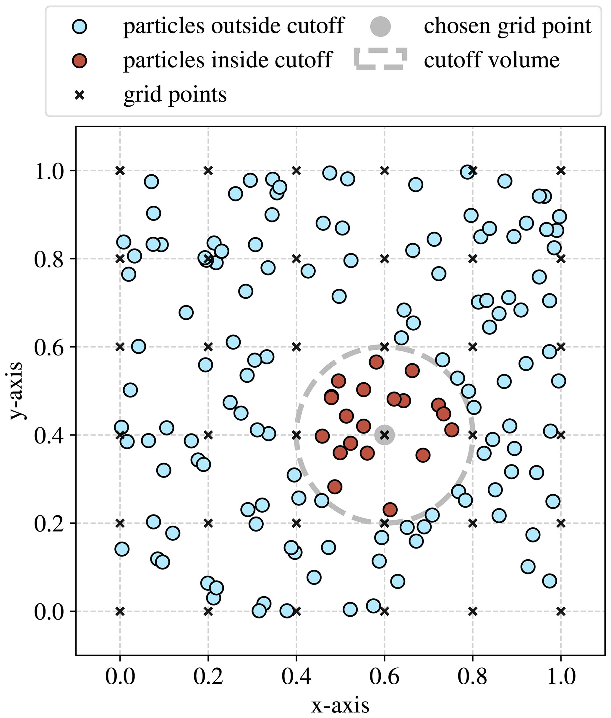
Figure 5 Visualisation of particle-to-node association. This plot displays an xy-plane projection of a synthetic set of particle positions in 3D (blue dots) within the framework of a regular grid (crosses). The particles associated with the grey grid point (red dots) are those within the cut-off volume (grey circle). The size of the dots is not informative of the size of the particles. For the sake of simplicity, no units are provided.

3.5.3 Weight calculation

The macroscopic continuum fields result from convolution of a microscopic discrete field with a CG (smoothing) function, Ψ, over the model space, thus performing a spatial weighted average of particle quantities. The smoothing function is defined by two parameters: the spatial domain, c, over which Ψ has non-zero values; and the effective smoothing width, w, which determines the spread or variance of Ψ, thereby controlling how particle contributions are spatially distributed within the volume of radius c.

Various kernel functions that may be employed in coarse-graining are implemented in Pysammos: the Lucy (Eq. 9), Gaussian (Eq. 10), and Heaviside (Eq. 11) functions. Different kernel forms relate c and w with different scaling factors. To provide a consistent comparison across kernels in Fig. 6, all functions are rescaled so that they share the same variance. This ensures that the differences between kernels are due to the function shape and not the difference in effective smoothing width w or the kernel spatial domain c.

$$\begin{array}{}\text{(9)}& \begin{array}{rl}\mathrm{\Psi }\left(r\right)& ={\displaystyle \frac{\mathrm{105}}{\mathrm{16}\mathit{\pi }{c}^{\mathrm{3}}}}\left(-\mathrm{3}{\left({\displaystyle \frac{r}{c}}\right)}^{\mathrm{4}}+\mathrm{8}{\left({\displaystyle \frac{r}{c}}\right)}^{\mathrm{3}}-\mathrm{6}{\left({\displaystyle \frac{r}{c}}\right)}^{\mathrm{2}}+\mathrm{1}\right)\\ & \text{if}r:=\left|\mathit{r}\right|<c\end{array}\end{array}$$

where c is the range of the weighting function and is usually set to c=2w for Lucy polynomials (Weinhart et al., 2013).

$$\begin{array}{}\text{(10)}& \begin{array}{rl}\mathrm{\Psi }\left(r\right)& =\exp \left(-{\displaystyle \frac{r^{\mathrm{2}}}{\mathrm{2}{w}^{\mathrm{2}}}}\right)\left[\mathrm{2}\sqrt{\mathrm{2}}{\mathit{\pi }}^{\mathrm{3}/\mathrm{2}}{w}^{\mathrm{3}}\text{erf}\right.\\ & {\left.\left({\displaystyle \frac{\sqrt{\mathrm{2}}}{\mathrm{2}}}{\displaystyle \frac{c}{w}}-\mathrm{4}\mathit{\pi }c{w}^{\mathrm{2}}\exp \left(-{\displaystyle \frac{c^{\mathrm{2}}}{\mathrm{2}{w}^{\mathrm{2}}}}\right)\right)\right]}^{-\mathrm{1}}\end{array}\end{array}$$

where the erf is the error function, and c=3w for the Gaussian weighting function.

$$\begin{array}{}\text{(11)}& \mathrm{\Psi }\left(r\right)=\left\{\begin{array}{ll}\frac{\mathrm{1}}{\mathit{\phi }},& r\le c,\\ \mathrm{0},& r>c,\end{array}\right.\end{array}$$

where $\mathit{\phi }=\frac{\mathrm{4}}{\mathrm{3}}\mathit{\pi }{c}^{\mathrm{3}}$ is the volume of a sphere with radius c. It follows that c=w in the Heaviside function.

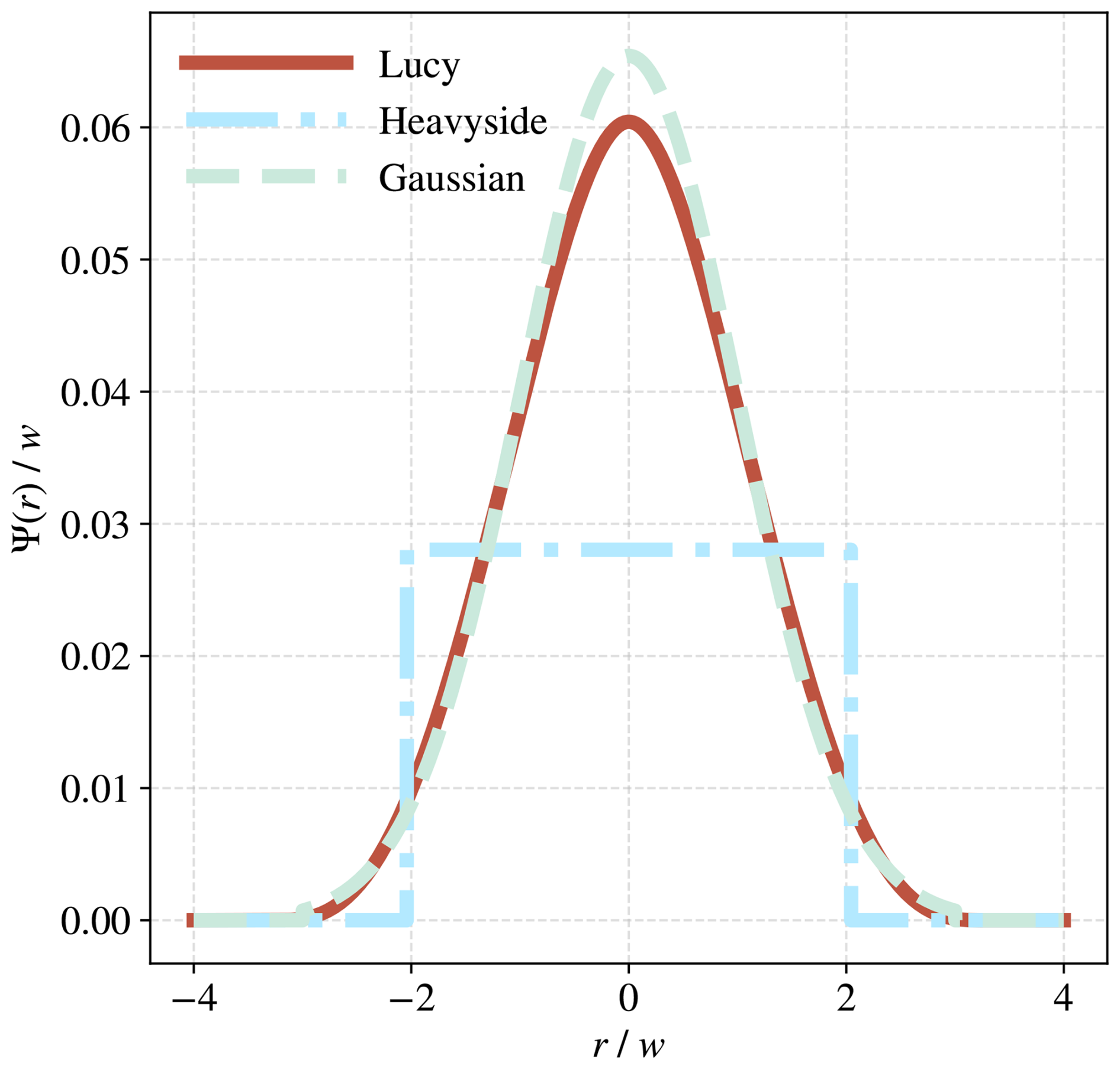
Figure 6 Visualisation of the three implemented coarse-graining weighting functions, Ψ(r), in one dimension (r) normalised by the effective smoothing width (w). Note that the functions have been plotted with equal variance in order to ensure that any differences are due to kernel shape, not scale.

The weights are pre-calculated for a range of particle-grid point distances, extending from 0 to c, and corresponding to a discretisation of space at a high enough resolution to ensure accuracy. This approach provides a more efficient performance as it avoids the redundant calculation of weights. It is carried out with a lookup table algorithm, details of which can be found in Appendix B3.

The calculation of contact-related fields (e.g., the contact stress tensor, Eq. (5) requires the additional line integral of Ψ along the branch vector connecting a particle centre to a contact point. This integral could, in principle, be solved analytically for each kernel individually (Weinhart et al., 2012). In Pysammos, we instead evaluate it numerically: the branch vector is discretised into N=10 points, sampled through the same lookup table employed for particle weights, and integrating with the trapezoidal rule. This provides a single, kernel-independent implementation of the integral. Increasing N beyond 10, up to 10⁵, produced no discernible change in the resulting contact stress fields (Fig. S7 of the Supplement), confirming that the trapezoidal integration is already converged at this resolution.

3.5.4 Macroscopic fields

The structure of the field computing functions consists of several nested levels of iterations. The outermost iteration, which is parallelised using Numba, is performed over the grid points, as it is the largest dimension. The next level iterates through the particles within the cut-off volume of that grid point. Subsequently, an iteration through phase is performed, if specified by the user. Finally, if the resulting field has more than one dimension (i.e., is a vector or a tensor), additional levels of iteration are implemented to carry out element-wise multiplication. Details about the utilisation of Numba in Pysammos can be found in Appendix E1.

A range of continuum fields can be calculated with Pysammos (Appendix C). To allow the user to customise what fields to export for a more efficient use of the tool, yet accounting for dependencies of required fields, an inbuilt tool is used in the user-interface class to determine the full set of fields that have to be computed given a series of user-selected fields to be exported.

3.6 Data writing stage

Pysammos provides two types of output files: a vtkhdf file per DEM time step processed, for ParaView visualisation; and a single h5 file containing data from all the time steps, for data analysis and storage. Vtkhdf files are built on hdf5 but are adapted for vtk-type workflows, thus combining the parallel I/O support and the optimisation for meshed structures with the standardisation of data storage for visualisation purposes. On the other hand, h5 files offer high flexibility for structured data storage, are optimised for large datasets, and are compatible across programming languages.

4 Results

In the following section we present the results concerning the benchmark of the code to other available CG software and the computational performance. We then provide an example of a user-friendly script to perform CG in Pysammos, and a series of examples to showcase the functionalities of the code for visualisation and analysis.

4.1 Benchmarking

Pysammos is intended to be used by a diverse community working with computational particulate methods, spread across geosciences, engineering and physics. Hence, reassuring users that it yields reliable results is key. For that reason, we compared results from Pysammos to other CG software: Iota-Suite (LeCroy, 2025), EDEM's continuum analysis (Altair Engineering, Inc., 2025), Granulysed (using Iota-Suite and VELaSSCo (Morrissey et al., 2020)), and MercuryCG (Weinhart et al., 2020a). We used a benchmark DEM sample of a static monodisperse cubic lattice with vertical plate displacement and fixed side walls. The particles have diameter d=0.02 m and density ρ=2500 kg m⁻³. The sample is analysed at the centre, $P=\mathrm{0},\mathrm{0},\mathrm{0.42725}$ m (Fig. 7g). The tests are carried out for different smoothing half-width lengths multiples of the characteristic particle size (i.e., $w/d$) and smoothing functions. These established tests are straightforward to carry out, as they are easily accessible through the user interface class. Future versions of the code should be benchmarked using the same data in order to guarantee output consistency. Figure 7 contains the continuum fields of the benchmarked simulation, computed with several different CG codes. All the fundamental continuum fields, including all the vector and tensor components are provided in the Supplement.

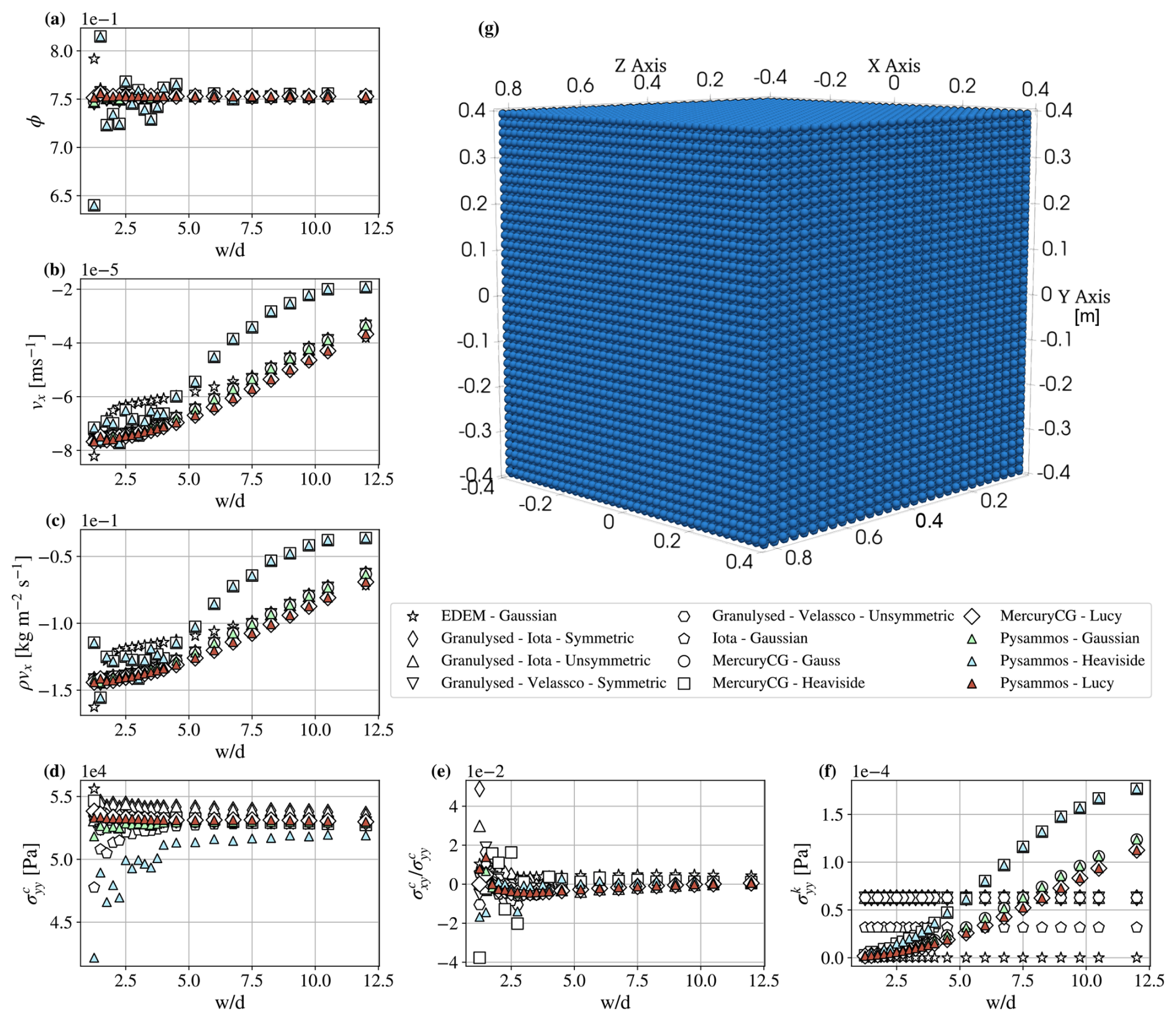
Figure 7 Benchmark of a monodisperse cubic lattice of grains with a diameter of 0.02 m and density of 2500 kg m⁻³ (g), at a point $P=\mathrm{0},\mathrm{0},\mathrm{0.42725}$ m. It was coarse-grained with Pysammos (coloured triangles) and other coarse-graining software (void shapes): EDEM, Granulysed, Iota, and MercuryCG. Different smoothing functions (Gaussian, Heaviside and Lucy), are compared when available, for a range of smoothing half-width lengths multiples of the characteristic particle size (i.e., $w/d$). The volume fraction is shown in (a). The horizontal component of the velocity and the momentum density are shown in (b) and (c), respectively. The vertical component of the contact stress is provided in (d), whereas (e) displays the ratio between the latter and the shear component in the xy-plane. Finally, the vertical component of the kinetic tensor is shown in (f).

Volume fraction is overall constant across the entire $w/d$ range (Fig. 7a). It shows a larger spread of values across codes in the lower range of smoothing widths when using the Heaviside functions in Pysammos and MercuryCG. The mixture density field shows a very similar set of characteristics to the volume fraction (see Fig. S1). The velocity (Fig. 7b) and momentum density (Fig. 7c) fields at the tested point increase as the smoothing width is increased for all codes. The Lucy function yields slightly lower values than the rest of the codes for $w/d>\mathrm{4}$, whereas the Heaviside functions and EDEM’s Gaussian consistently estimate higher values. Pysammos’s results coincide with MercuryCG's corresponding results, as they use the same weighted spatial averaging scheme. The kinetic tensor field increases overall as the smoothing width is enlarged (Fig. 7f). Granulysed calculations yield constant values of the kinetic tensor across the entire $w/d$ range. The results rendered by Pysammos, coincide again with those from MercuryCG.

The contact tensor field (Fig. 7d) shows a broadly constant mean value across the analysed $w/d$ range (see Fig. S6e for enlarged view), with a greater scatter at the low end. Pysammos and MercuryCG show a degree of discrepancy at lower $w/d$. This could be attributed to the difference in the particle-search criterion between the two codes: in Pysammos, a contact is included in the averaging volume based on the distance from the grid point to the centre of particle i, whereas MercuryCG's determines inclusion based on the minimum distance from the grid point to the branch vector itself (Weinhart et al., 2020b). This more general criterion allows MercuryCG to include contacts whose branch vector is positioned near the grid point even when the particle centre itself lies outside the cut-off radius, an effect expected to be more pronounced at low $w/d$, where the search radius is comparable to the branch-vector length. We note that this discrepancy is unlikely to stem from the numerical evaluation of the branch-vector line integral in Pysammos (Sect. 3.5.3), as the trapezoidal integration is already converged at N=10 sampling points (Fig. S7 of the Supplement) and is not expected to be a significant source of error even at low $w/d$. Further, the Heaviside function in Pysammos shows larger disagreement with that of MercuryCG across the whole $w/d$ range and especially in the diagonal components of σ^c, compared to the off-diagonal ones (see Fig. S5). This could be due to the Heaviside's uniform weighting of all the particles within the search volume, which exacerbates edge effects of the search shift discussed above. Conversely, the Gaussian and Lucy functions heavily damp the contribution from particles further from the evaluation point, making them less susceptible to this issue. Despite these discrepancies, the ratio of the vertical to the shear component in the xy-plane of the contact stress tensor converges towards a constant value close to 0 after $w/d\sim \mathrm{3}$, whereas it shows a larger scatter on the order of $\pm \mathrm{4}\times {\mathrm{10}}^{-\mathrm{2}}$ for $w/d<\mathrm{3}$ (Fig. 7e).

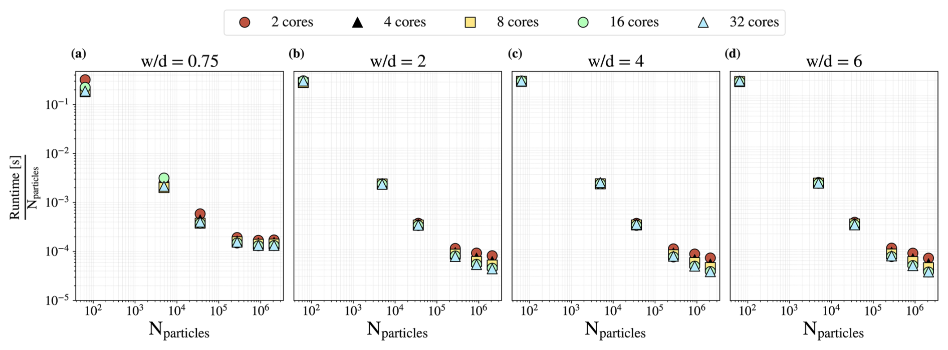
Figure 8 Computational cost per particle, and per time step, as the dataset size increases using a different number of CPUs for parallelisation. The cost per particle is measured as the runtime duration (in seconds) normalised by the number of particles within the region of the model being processed. The performance was compared across different search radii, $w/d$: the default 0.75 (a), 2 (b), 4 (c) and 6 (d).

4.2 Performance

The computational performance of Pysammos's CG workflow was evaluated by means of the computational cost per particle as the post-processed model increased in size. The computational cost per particle corresponds to the ratio between runtime and number of accounted particles, and it is a measure of how well the code scales resources needed as complexity increases. The model size is quantified by the number of grid points and/or particles in the analysed space. The performance was tested at different spatial averaging resolutions ($w/d$), and using different number of core processors. Thus, we provide a map of optimal performance across different analysis scenarios, revealing that the ideal configuration depends on the nature of the data being processed and the resolution at which it is being processed.

The DEM sample was that of a static random packing cube of side length ∼95d₄₃, with a high coordination number of ∼5–6 (Fig. 10 prior to the impact). All available outputs, involving both particle and contact related fields, were exported in order to have a complete representation of the computational requirements when running the program at full capacity. The quoted runtime values are an average of three different computed time steps. The computation for this exercise was carried out on the ARCHER2 HPC cluster.

The cost per particle decreases sub-linearly with number of particles across all averaging resolutions and number of cores, meaning the code cost scales favourably with problem size (Fig. 8). This entails that overheads are being amortised and caches are being used efficiently. Inherently, for a given tested model size (i.e., N_particles), the higher the CG resolution is (i.e., lower $w/d$), the larger the number of grid points, but the fewer particles per grid point. Consequently, we observe that across all number of cores, the cost per particle at Pysammos's default $w/d=\mathrm{0.75}$ begins to plateau at $\sim {\mathrm{10}}^{-\mathrm{4}}$ for 10⁶ particles (Fig. 8a), but for larger $w/d$ it continues to decrease (Fig. 8b–d). Thus, we can say that the number of particles per grid point controls the point at which the performance plateaus. At higher resolutions, the iteration at each grid point carries out operations across a smaller range of particles, which is harder to amortise for large models (∼10⁶ particles), regardless of the total number of grid points.

The use of parallel computing reduces the cost per particle for model sizes of N_particles>10⁵ at resolutions of $w/d>\mathrm{2}$ (Fig. 8). The efficiency gained from additional cores increases with $w/d$, up to $w/d=\mathrm{6}$, beyond which it begins to plateau relative to $w/d=\mathrm{4}$ (Fig. 8c, d). For larger systems (N_particles>10⁵) the speed-up by parallelisation saturates at a low number of cores under sub-particle resolution, but at 16 cores for w>d. For smaller systems (N_particles<10⁵), parallelisation provides no noticeable speed-up at resolutions w>d, and saturates at a low number of cores (∼2) at resolutions w<d. Although Numba reduces Python-level overhead, the gains from additional parallelism at w<d are of limited improvement (Fig. 8a), most likely because the algorithms where Numba parallelisation is employed are memory-bound, and this cost is not sufficiently amortised when the number of particles per grid point is small.

Therefore, when coarse-graining at a high resolution below the particle scale, it is recommended to use a low number of cores to attain optimal computational efficiency. Nevertheless, this means that efficient execution of Pysammos does not require extensive parallel resources, thereby making this post-processing software well suited for shared computational systems. On the other hand, when coarse-graining at a lower resolution, namely above particle scale, in a large dense packing it is recommended to use between 4 and 16 cores. In general, further improved parallel performance can be attained by, alternatively or additionally, distributing independent time slices across different shared-memory processes.

4.3 User-friendly workflow

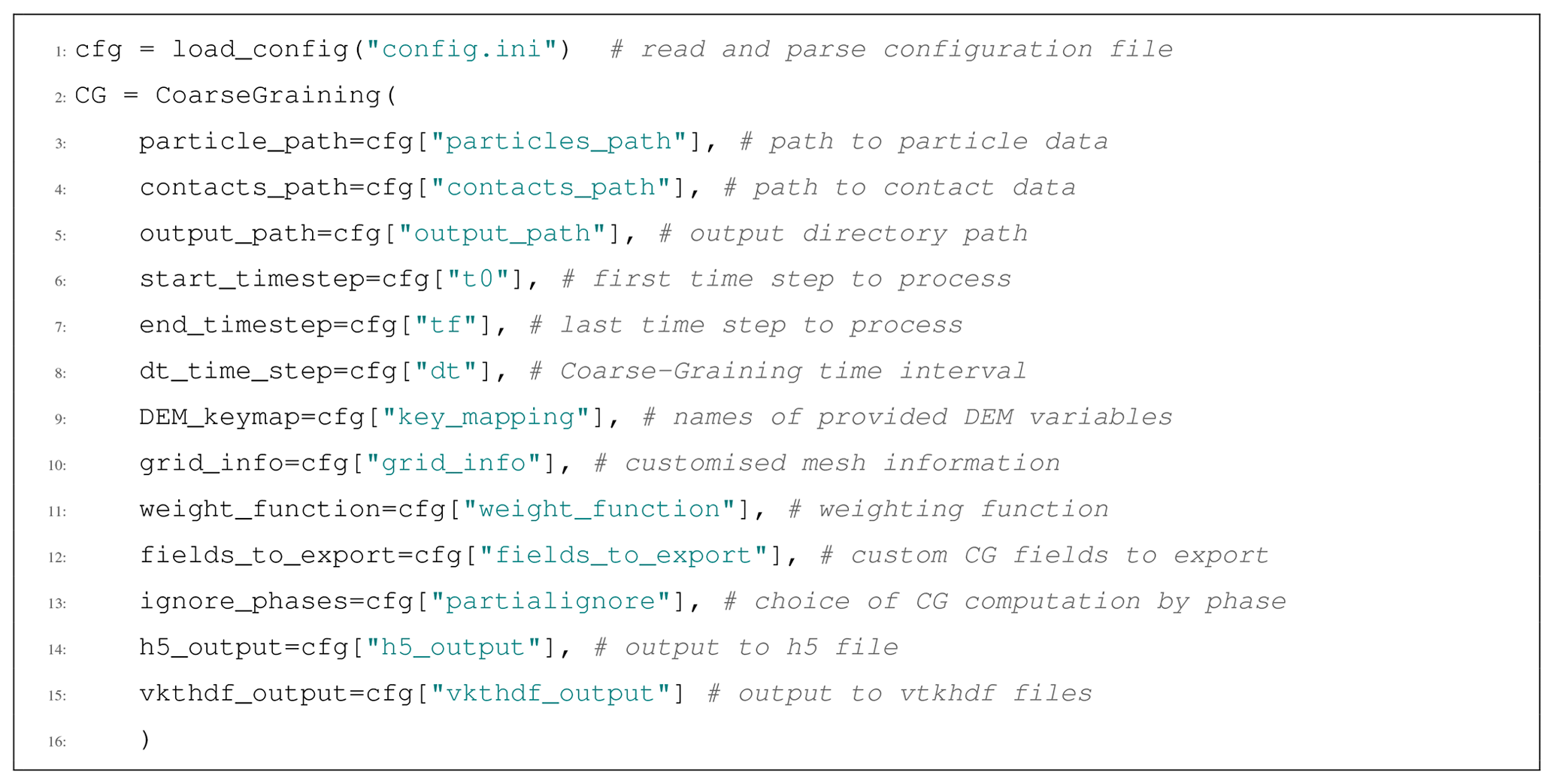
Here we provide a usage example of the user-facing CoarseGraining class. Listing 1 shows how to initialise the class with the entries of the configuration file. See Appendix A for an example of a configuration file.

Listing 1 Initialisation of the CoarseGraining class.

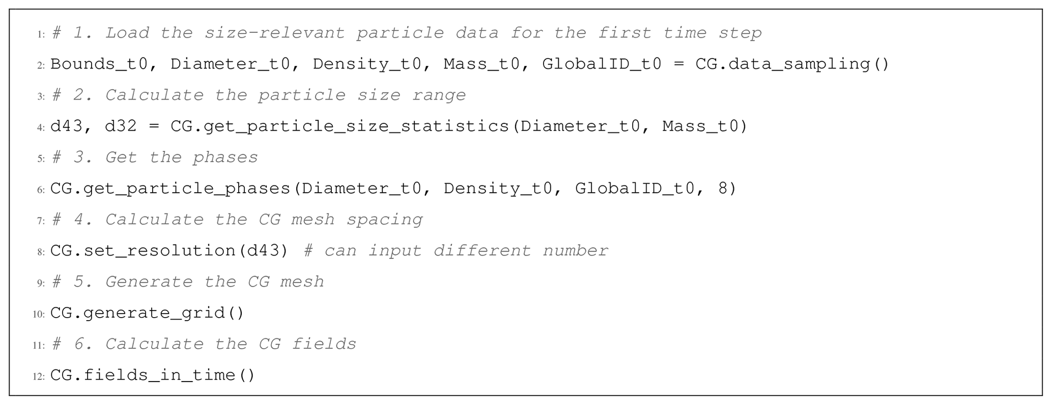
Listing 2 presents the algorithm steps of the CG workflow applied through the methods of the CoarseGraining class, previously described in Sect. 3. Alternatively, the method CG.run() performs all the steps sequentially with default parameters.

Listing 2 Coarse-graining workflow with Pysammos.

4.4 Example cases

Below we present a set of example MFiX DEM simulations of processes relevant to the geoscientific community, alongside coarse-graining results to showcase the functionalities offered by Pysammos – some of the various continuum fields that can be computed, relevant further data analysis, and result visualisation modalities.

4.4.1 Bedload transport

The following example demonstrates how Pysammos can process a polydisperse mixture of non-spherical particles in a 2D model, and provide ParaView-ready outputs. It also provides an insight into the breadth of information that can be obtained using DEM and Pysammos's coarse-graining for the study of river bedload transport.

Figure 9 displays a DEM-CFD 2D numerical simulation representing bedload sediment, of polydisperse non-spherical grains, submerged in water over a rough static base of spherical grains. The boundaries of the x axis are made periodic. The water is subjected to periodic horizontal planar waves travelling in the positive x direction. The time step in Fig. 9 captures wave fronts at x∼0.05 m and x∼0.45 m. These are manifested as bands of higher shear rate (Fig. 9d) and inertial number I (Eq. C19), a measure of the dynamic state of a granular medium further described in Appendix C2 (Fig. 9c). However, the wave fronts do not appear obvious in the contact network (Fig. 9b). It can also be seen that shear rate decreases with depth, as expected in bedload transport (Houssais et al., 2015).

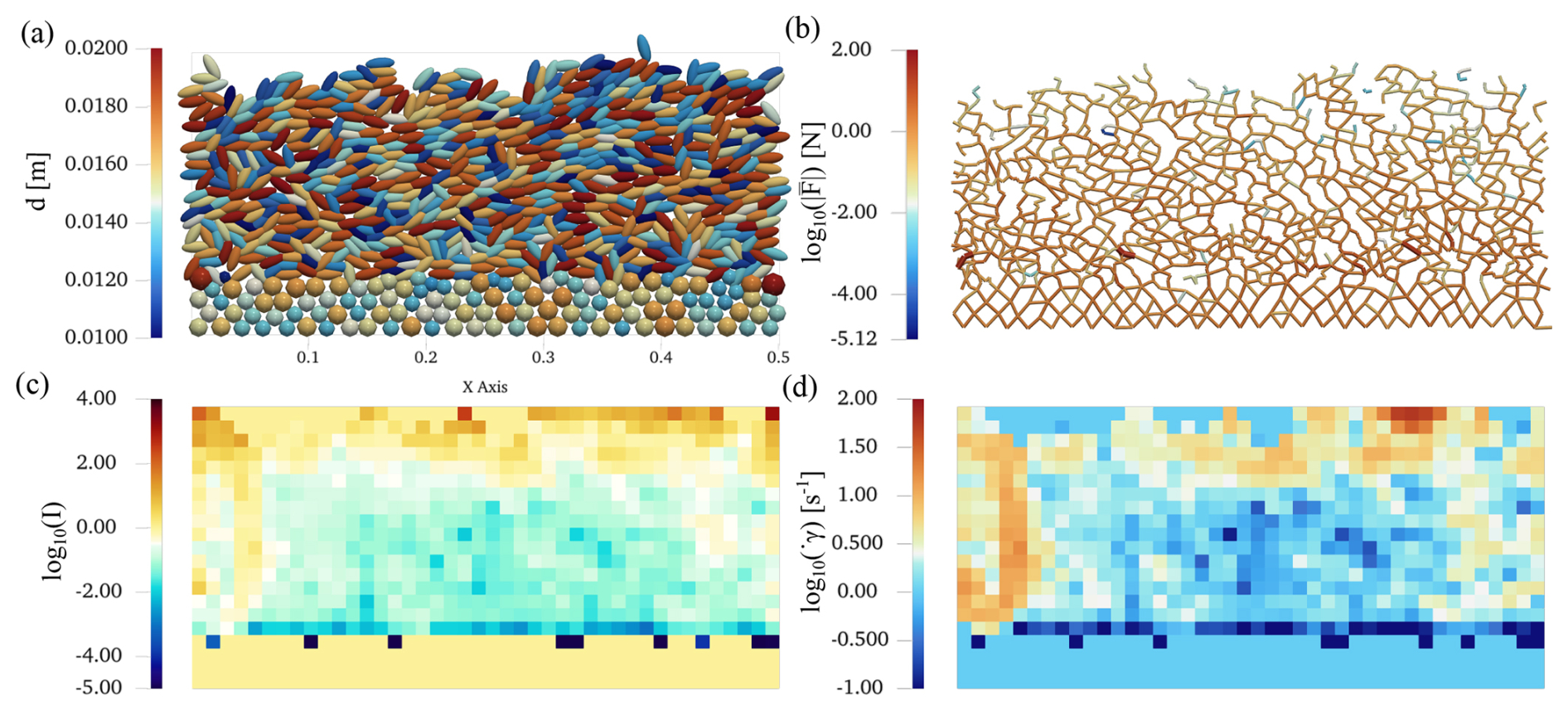
Figure 9 DEM-CFD 2D numerical simulation representing bedload sediment, of polydisperse non-spherical grains, submerged in flowing water over a rough static base of spherical grains (a). The water is subjected to periodic horizontal planar waves in the positive x direction. The contact network is shown in (b) and is coloured by the normalised force magnitude ($\left|\overline{F}\right|$). Plots (c) and (d) display the inertial number (I) and shear rate tensor magnitude ($\dot{\mathit{\gamma }}$) coarse-grained fields evaluated with Pysammos, respectively.

4.4.2 Impactor on polydisperse granular bed

This example illustrates the ability of Pysammos to recover high spatial resolution fields from a large DEM model (∼10⁶ particles). We present a DEM simulation of a high-speed impact on a granular bed, as a case study relevant in the field of both extraterrestrial cratering and seismology. It consists of a cuboid polydisperse bed ($\mathrm{0.08}\times \mathrm{0.08}\times \mathrm{0.08}$ m), struck at high speed by a large impactor (d_L=0.001 m) (Fig. 10). The particle diameters were drawn from a normal distribution with a mean of 0.0008 m and a coefficient of variation of 10 %.

Vertical slices in the xy-plane (at z=0.04 m) of the contact network and several coarse-grained fields at a spatial resolution similar to the particle size are shown in Fig. 11. The contact network is less dense in the vicinity of the impact due to particle ejection, with higher magnitude forces (∼ 10⁶ N) within a sphere around the impact (Fig. 11a). The vertical component of the velocity shows the shock wave propagating downwards (Fig. 11b). In addition, we see two paths of lower particle velocity radiating outwards from the impact towards the side walls. This, however, is not observed in other fields, such as pressure (Fig. 11c) or inertial number (Fig. 11d), where the shock wave is seemingly mostly isotropic and has the same radial extent as that seen in velocity. Figure 11e displays the μ(I) according to GDR MiDi (2004), to assess the extent to which the rheology of the mixture can be approximated to a local rheology, if the background blue is the static coefficient of friction of this mixture (∼ 0.4). In fact, we see that μ(I) is greater than the coefficient of static friction around the region of impact, which is what has been observed in the literature at high values of inertial number – in this case corresponding to high pressure – (Barker and Gray, 2017). Finally, the coordination number (i.e., the number of contacts of a given particle) is plotted in Fig. 11f, from which we can see a decrease towards the region of impact, and a faint ring of lower coordination number at the wave front.

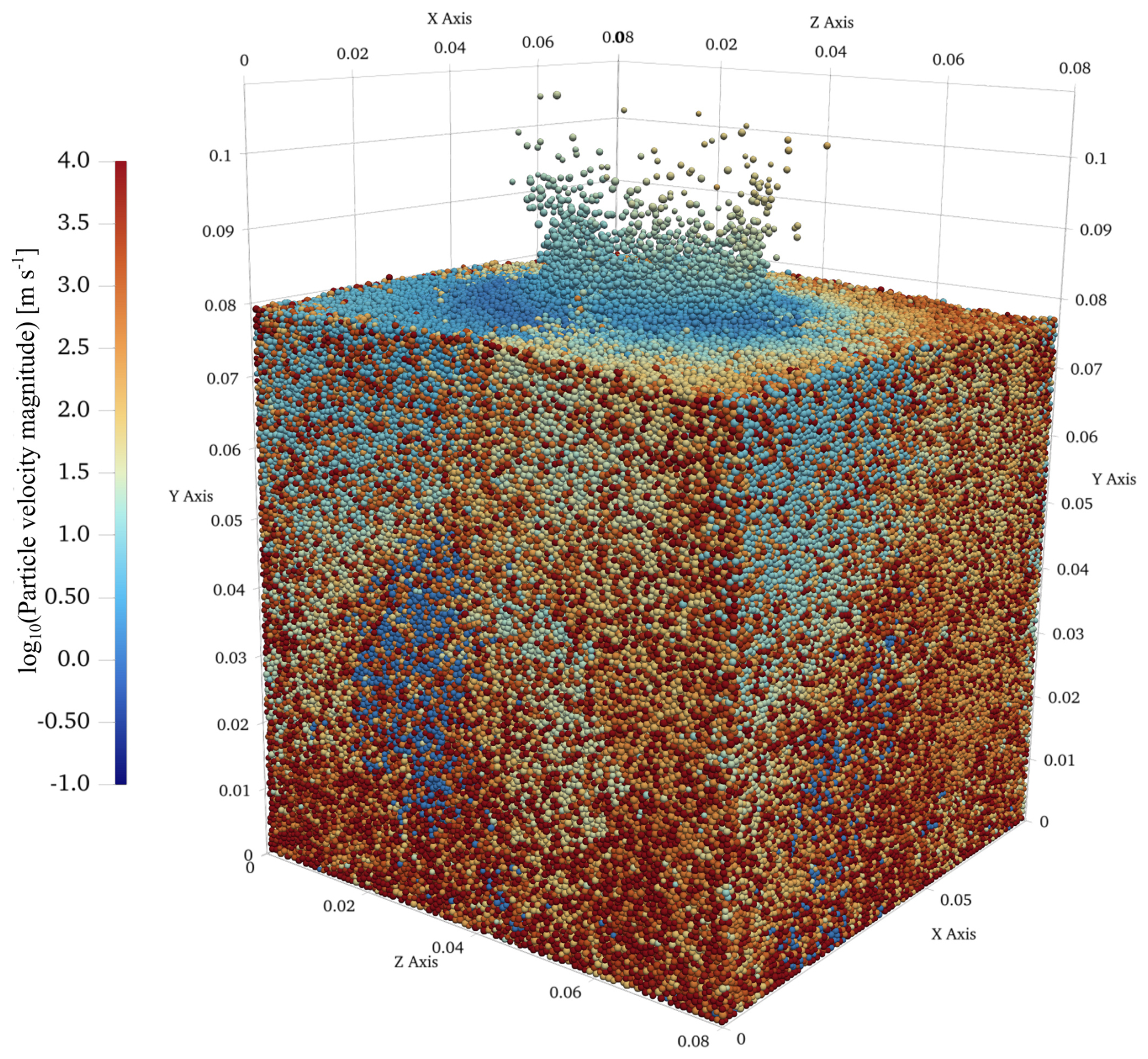
Figure 10 DEM numerical simulation of a polydisperse cuboid bed, of spherical particles initially at rest, hit at high velocity by an impactor larger in size.

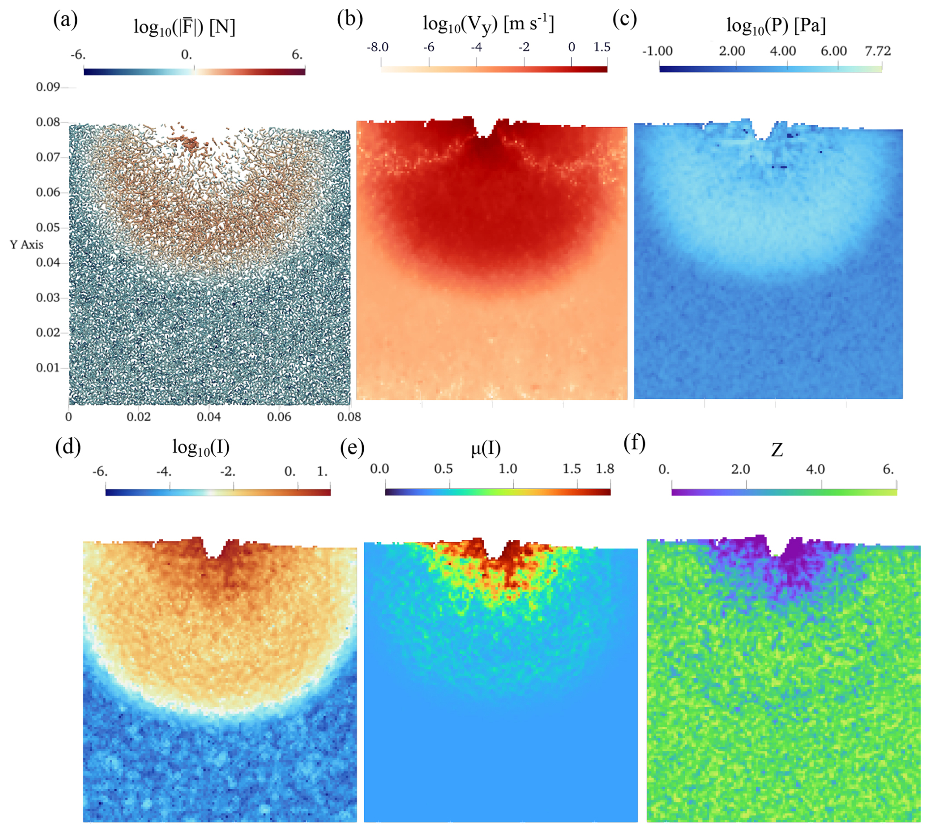
Figure 11 Vertical slices in the xy-plane (z=0.04 m) of the coarse-grained fields corresponding to the DEM numerical simulation of a polydisperse bed hit by an impactor presented in Fig. 10. The contact network is shown in (a), coloured by the normalised force magnitude ($\left|\overline{F}\right|$). The vertical component of the velocity (V_y), pressure (P), inertial number (I) and coordination number (Z) are displayed in (b), (c), (d) and (f), respectively. The coefficient of friction as a function of inertial number (i.e., μ(I)-rheology) is shown in (e), where the static coefficient of friction of the mixture (∼ 0.4) is coloured light-blue.

4.4.3 Crystal suspension in magmas

This example showcases the application of Pysammos to granular suspensions, that is, particles flowing and interacting with each other and the fluid they are immersed in. The rheology of granular suspensions controls the dynamics of lava flows and magma reservoirs (McIntire et al., 2019), and has begun to be studied with DEM (Qin et al., 2020).

Hence, we present a DEM-CFD pseudo-2D (i.e., with a thickness of one cell) numerical simulation representing non-spherical crystals suspended in magma flowing cyclically in the positive vertical direction through a narrow conduit with frictional walls (Fig. 12a). The particles are fully three-dimensional and interact with the fluid through a two-way coupling via drag and pressure forces. The flow is driven by a constant flux, causing the particles to accelerate until they eventually reach steady state. Given the sparsity of the solid particles, we chose a smoothing function half-width four times larger than the default option, 0.75 ×d₄₃.

The interstitial fluid was made viscous to resemble magma. However, the viscosity (10 Pa s) was chosen to be significantly lower than that of magmas (10⁻¹–10¹⁴ Pa s, Giordano et al., 2008) to decrease the computational cost of the simulation, as the purpose is to demonstrate the application to this field. The viscous number, $J=\dot{\mathit{\gamma }}{\mathit{\eta }}_{\mathrm{f}}/P$, where η_f is the viscosity of the interstitial fluid, is commonly used in the study of granular suspensions (Boyer et al., 2011) and it is plotted in Fig. 12b. The viscosity is higher on the sides due to frictional forces at the conduit walls, also shown to slow down the particles (Fig. 12a).

The dimensionless effective shear viscosity, ${\mathit{\eta }}_{\mathrm{s}}=\mathit{\mu }/J$, measures the competing shear viscosity from the particles and the fluid itself (Boyer et al., 2011). In Fig. 12c η_s<1, implying that the presence of particles lowers the viscosity of the fluid. However, in Fig. 3 of Boyer et al. (2011), η_s<1 for ϕ<0.3. Therefore, for the low concentration of suspended particles (ϕ≪ 0.1) used in this example (see Fig. S9 of the Supplement), very low effective shear viscosity is to be expected.

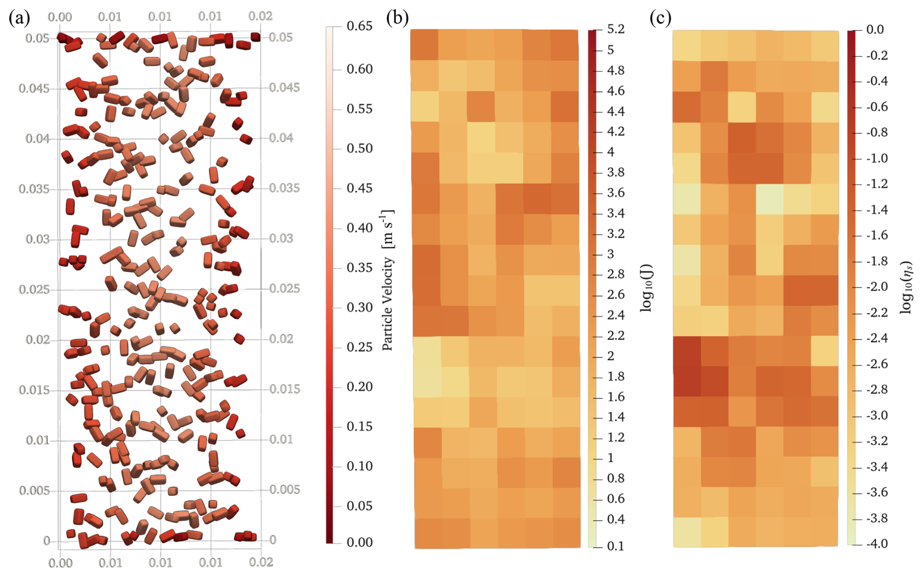
Figure 12 DEM-CFD 2D numerical simulation representing non-spherical crystals suspended in magma (a). The interstitial fluid was made viscous to resemble a magma mush. However, the viscosity was chosen to be significantly lower than that of magma to decrease the computational cost of the simulation, as the purpose is to demonstrate an application. The coarse-grained fields of the viscous number ($J=\dot{\mathit{\gamma }}{\mathit{\eta }}_{\mathrm{f}}/P$, where η_f is the viscosity of the interstitial fluid), and dimensionless effective shear viscosity (${\mathit{\eta }}_{\mathrm{s}}=\mathit{\mu }/J$) are presented in (b) and (c), respectively.

4.4.4 Pile-stabilised slopes

This example highlights the package's ability to (1) analyse and visualise Pysammos results entirely in Python, (2) resolve individual phases within a polydisperse mixture, and (3) straightforwardly assess each phase's contribution to the bulk properties of the mixture. DEM can also be used to study vertical load redistribution in loose sediment – for instance, in debris-flow deposits posing a risk to nearby communities and infrastructure. Here, we present a 2D DEM simulation of a growing granular pile, in which grains of different sizes are poured from above into a confined space between two walls 50 cm apart (Fig. 13a). This model captures two combined effects: force-chain arching in a free-surface granular pile (Brockbank et al., 1997), and the Janssen effect, whereby vertical stress saturates with depth as it is redistributed laterally through friction at the side walls (Windows-Yule et al., 2019).

Through this example we see that, near the peak of the pile, basal pressure exhibits a local minimum, rather than the maximum that a hydrostatic gradient of a fluid would predict directly beneath the peak (Fig. 13d) – a phenomenon that has been documented experimentally (Brockbank et al., 1997). This occurs because granular assemblies transmit stress anisotropically along chains of contacting grains, rather than isotropically as in fluids, redirecting stress sideways by “arching” it toward the flanks of the pile rather than accumulating it directly underneath. These arching structures are visible as high-magnitude bands in the total stress tensor magnitude field (Fig. 13b). This effect is even more pronounced in this 2D configuration, compared to a 3D pile.

The mechanism behind this stress redistribution is more explicitly shown by the shear stress field (Fig. 13c). Unlike the stress magnitude, which illustrates where stress locally intensifies, the sign of the shear stress specifies the direction in which load is being carried: shear stress is close to zero along the vertical centreline and grows with opposite sign toward each flank. This indeed confirms that weight is transported away from the pile’s apex in both lateral directions, rather than straight downward. The largest shear stress magnitudes do not occur at the side walls, but midway between the peak and the walls. This is consistent with force chain curving outward and downward through the pile before reaching the walls. This suggests force chain arching is probably the dominant redistribution mechanism here, with the walls providing at least a partial frictional contribution to support, consistent with a weakly-developed Janssen effect. This is visible in Fig. 13e, where in the wall-confined region (heights of 0.005–0.03 m), horizontal stress increases with depth while vertical stress remains constant – indicating that the walls are supporting part of the pile's weight. We note that this apparent depth-independence of vertical stress is not expected to persist as the pile height grows, given that the wall-supported fraction of the total weight would saturate, while the unsupported fraction below saturation depth would grow with height approximately following a hydrostatic profile. Finally, we find that the different phases identified by grain diameter contribute differently to the bulk stress at different heights, although the relatively low polydispersity of this mixture means all phases contribute roughly equally to the bulk field along the profile.

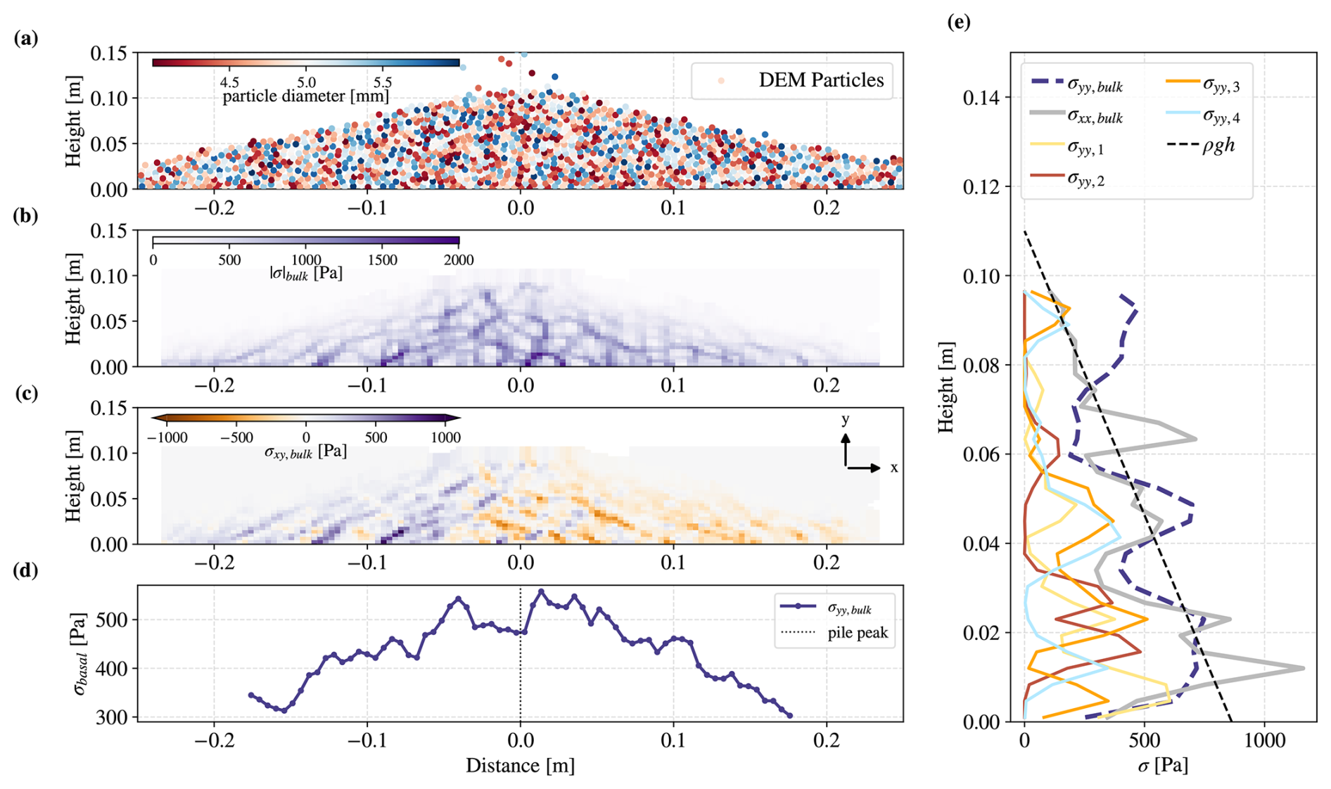
Figure 13 Analysis of a 2D DEM simulation of a growing granular pile carried out with Pysammos's Python-supported visualisation. Simulation particles coloured by size (a), coarse-grained magnitude of the total stress tensor (b) and shear stress (c) across the granular mixture. Coarse-grained basal vertical stresses, taken from the lowest row of CG cells, as a function of horizontal distance, testing for stress arching beneath the pile crest (dotted black line, x=0) (d). Vertical profiles, taken along the pile centre (x=0) dotted line in (d), of the horizontal stress of the mixture (grey solid line), vertical stress of the mixture (dashed blue line), and vertical stress of each of the phases with diameters 5.7, 4.7, 5.1, and 4.2 mm, in yellow, red, orange and blue, respectively (e).

4.4.5 Erodible granular beds

The following example showcases a feature of Pysammos that provides profiles of the coarse-grained fields along a given axis, averaging over the other two axes. This is suitable for post-processing DEM simulations that are close to constant in the directions in which the data are averaged, and show transient or gradual characteristics in the direction in which the profile is produced. To illustrate this functionality, we present a DEM simulation of a monodisperse granular column, over an inclined (24°) rough base, sheared at the top by a rough plate, approximating the effect of an overriding flow (Fig. 14a). The simulation was initially run with a fixed erodible bed until the overriding flow reached steady state, after which the bed was allowed to be mobilised by the flow.

Vertical profiles of the horizontal granular temperature (T_x), calculated according to Eq. (C13) and alternative slice-averaging approaches (Zhang and Kamrin, 2017; Plimpton, 1995), are averaged over the last second of erosion and shown in Fig. 14c. The three methods are in agreement along the profile up to the height at which the flow becomes more dilute (Fig. 14b), where the results yielded by the slice methods depart from Pysammos's.

The overall trend shows an increase of T_x with depth. In other words, towards the top of the column the particle velocity is more correlated to the velocity mean field. This implies that the erodible bed has been mobilised and entrained into the flow, and the bottom part is rattling as the rough base is hindering movement. This is manifested in the flow velocity as a typical Bagnold profile (Fig. 14e), where most of the column is flowing at a constant velocity, affine to that of the overriding flow, below which there is a shear zone driven by geometric friction induced by the rough-frictional base.

The instantaneous profiles, taken at a frequency of 10 Hz, are shown to oscillate by several orders of magnitude about the time averages of the first and last seconds of erosion (Fig. 14d). Nevertheless, it is clear that it is a transient process, migrating from a shallow gradient to a steeper gradient with height, implying a dissipation of granular temperature through the column due to friction at the base. This is also seen in the velocity profiles, as the steady state is attained in the form of a Bagnold profile.

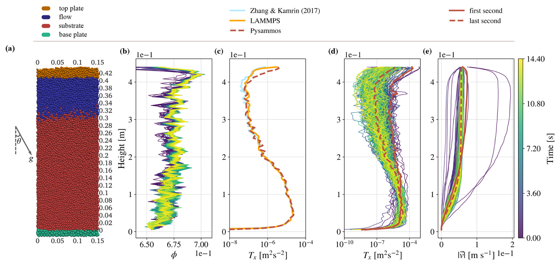
Figure 14 DEM simulation describing a tilted erodible granular column (24°) sheared by a rough plate at the top, approximating the effect of an overriding flow (a). Instantaneous vertical profiles of the coarse-grained volume fraction, φ (b). Time averages of alternative calculations of the horizontal component of the continuum granular temperature field, T_x, such as that presented in Zhang and Kamrin (2017), and that implemented in LAMMPS (Plimpton, 1995) (c). Instantaneous vertical profiles of the horizontal granular temperature (purple-yellow) shown alongside the time averaged profiles corresponding to the first (solid red) and last (dashed red) seconds of simulation (d). Instantaneous vertical profiles of velocity magnitude, $\left|\mathit{V}\right|$, shown alongside the average over the first (solid red) and last (dashed red) seconds of simulation (e).

5 Discussion

In this section we discuss the strengths and limitations of Pysammos and hence recommend practices when employing it, as well as reflecting on the contributions to the DEM community, and outline the ongoing work and paths for future work.

5.1 Recommended practice: strengths and caveats

5.1.1 Choice of smoothing function

The benchmark of Pysammos against other codes shows that the CG fields are congruent with those obtained from other software. The results from the Gaussian and Lucy smoothing functions show similar results, whereas the fields calculated with the Heaviside function have a larger spread and offset on some occasions. This could be due to the fact that the Heaviside function weights all the particles within the search diameter equally hence exacerbating edge effects, whereas the Gaussian and Lucy functions heavily damp the contribution from particles further from the evaluation point. Nevertheless, the Gaussian function in Pysammos has an imposed cut-off, making it not perfectly smooth and thus non-differentiable, violating the condition that must be satisfied by the differential conservation equations (Babic, 1997). Therefore, we recommend the Lucy weighting function over the Gaussian and Heaviside functions.

5.1.2 Choice of smoothing width

The choice of smoothing width, w, is not trivial. Weinhart et al. (2013) show that the CG fields are independent of the smoothing width for a finite range of w values, which in turn vary with flow regimes and time averaging windows. For case studies exhibiting flow regimes ranging from quasi-static to inertial, as observed in natural flows, studies find that a $\mathrm{0.5}<w/d<\mathrm{1.5}$ is suitable to capture stable results in all the zones corresponding to the different flow regimes (Goldenberg et al., 2006; Weinhart et al., 2013). Hence, in Pysammos we have implemented a default value of w to be w_default=0.75d₄₃, used in most of our examples. Anyhow, we highlight the importance of investigating the stability of the obtained results given the employed w on the user's specific case study.

Glasser and Goldhirsch (2001) showed that the kinetic tensor is intrinsically dependent on the smoothing width (∼w²), due to the captured velocity gradients between the particle position and the point at which the CG fields are evaluated. The kinetic tensor can be decomposed into a scale-independent and scale-dependent components. The scale-independent contribution involves the local fluctuation velocity ${\mathit{V}}_i^{*}$ (Eq. 7), and is used to evaluate granular temperature, as this is a quantity that captures the particle's perspective. The scale-dependent contribution arises from velocity gradients in the coarse-grained velocity field. Although a scale-independent kinetic tensor would be desirable (Weinhart et al., 2013), the velocity gradients causing the scale dependence contain valuable information about the stress state and are therefore necessary for evaluating the total stress tensor.

In the example of granular suspensions (Sect. 4.4.3), we chose w=4w_default given the low volume fraction of the mixture. In doing so, when computing contact-related fields, such as pressure, the code averages nearby contacts where there are no particles, and vice versa. This might result in some artefacts and it should be accounted for in the result interpretation. For this reason, while we are confident in the robustness of Pysammos when applied to dense granular mixtures, we do recommend the user be rigorous when assessing the implications of the CG results of a dilute granular flow according to the mathematical formulations behind the software.

5.1.3 Phase detection algorithm

Mixture theory conceives granular mixtures to be populated by all phases with associated partial macroscopic fields contributing to a bulk field, where a phase can be defined as any particle property, or combination of properties, such as density, size, shape, elasticity, roughness (Tunuguntla et al., 2017).

In Pysammos we consider a phase to be defined by particle diameter and density, since they are two properties directly related to the two main competing mechanisms in segregation – kinetic sieving and buoyancy (Drahun and Bridgwater, 1983; Tripathi and Khakhar, 2013) –, ubiquitous processes in natural flows. Nevertheless, we would like to stress that this is a developer's choice of phase definition, and that the users should consider if this feature is relevant for their research.

The phase detection algorithm is based on clustering separation, which has been reported to perform better in clearly separated, round clusters (MacQueen, 1967). Hence, in granular mixtures with low polydispersity the phase detection algorithm would struggle to separate the mixture into phases, yielding arbitrary phases that depend on the choice of minimum number of clusters.

On the other hand, highly polydisperse mixtures would have to be handled carefully, as the smoothing widths depend on the characteristic particle size of the mixture. For instance, a large proportion of large particles might shift that average upwards, resulting in a smoothing width that could potentially obscure small particle behaviour. Therefore, we recommend the user to be cautious when coarse-graining polydisperse mixtures and perform stability and verification tests to ensure relevant and reliable information is being recovered.

From an implementation standpoint, phase detection is only performed on the first time step, producing a phase-ascribed array that is used to classify particles into phases in the subsequent time steps. If the polydisperse calculation of CG is applied to open systems (e.g., new particles are incorporated throughout the simulation), the phase array can no longer be matched to the particle data, as they will have different lengths.

5.1.4 Coarse-graining non-spherical grains

The mathematical foundation of the weighted spatial average implemented in Pysammos makes no assumptions about the shape of the particles (Babic, 1997). Hence, we are able to coarse-grain particles of any shape, as we have shown in the Results section. DEM software like MFiX – for which Pysammos is principally conceived – exports particle properties and information, including the total force and the geometric centre of the overlapping volume (Gao et al., 2022). Notably, Pysammos requires the total force between particle pairs, an export that is available only from MFiX-25 onwards.

The current MFiX release also supports the representation of irregular shapes via glued-sphere particles (GSP) (Lu et al., 2021). However, rather than exporting data for the individual bounding GSP – as required for CG in Pysammos – the current release exports data for the component spheres only. This limitation is being actively addressed in collaboration with the MFiX team, and in the interim, component-sphere data can be coarse-grained at the GSP scale to yield reasonable results. Section 5.3 illustrates what is currently achievable and outlines forthcoming capabilities.

5.1.5 Coarse-graining near the boundaries

Pysammos accounts for particles being positioned near cyclic boundaries, hence being in contact with particles at the opposite edge of the model, by calculating displacements to the nearest periodic equivalent. For that reason, we can say it is safe to generate a mesh as wide as the extent of the model between periodic boundaries, as long as the cyclic axes are provided in the configuration file. On the other hand, Pysammos does not take into account the effect of hard boundaries in the contact stress tensor, as described in Weinhart et al. (2012). Therefore, we advise users to avoid including particles in contact with walls in the extent of the generated mesh by entering suitable axes mesh ranges in the configuration file.

5.1.6 Optimal resource request

Concerning the efficiency of the program as it uses more cores, we see that the benefit of additional parallelism depends strongly on the coarse-graining resolution and system size. Although Numba reduces overhead, gains from additional cores at sub-particle resolution (w<d) are limited, most likely due to the memory-bound nature of the algorithms to which Numba is applied, where the number of particles per grid point is too small to sufficiently amortise this cost.

The optimal resource request therefore depends on the coarse-graining resolution. At high resolution (w<d), a low number of cores (e.g., 2) is sufficient to attain optimal computational efficiency. At lower resolutions (w>d), parallelism provides more substantial gains – for the dense granular packings considered here, between 4 and 16 cores is advisable for large systems (N_particles>10⁵). It is worth noting that this guidance is specific to dense packings and may vary for sparser or more heterogeneous systems.

In either case, efficient use of Pysammos does not require extensive parallel resources, making it well suited for shared memory computational systems. Enhanced parallel performance can further be attained by distributing independent time slices across different shared-memory processes – either as an alternative to, or in combination with, increasing the number of cores assigned to a single task.

5.2 Contributions to the DEM community

The DEM community is inherently interdisciplinary due to the ubiquity of granular processes in nature, engineering and industry. This naturally prompted the development of a range of DEM software, both open and closed source. In academic research open-source software is favoured from an ethical point of view. However, some open-source DEM software packages do not offer CG post-processing functionalities (e.g., MFiX), leading to the production of individual codes that do not tend to be widely shared, hindering reproducibility and increasing the likelihood of error propagation. Other DEM software might employ other averaging methodologies (e.g., LAMMPS, YADE). Stand-alone CG software might find their flexibility is limited by data format diversity (e.g., MercuryCG), forcing the user to convert data files. Recent efforts in the DEM community focus on standardising workflows and interoperability-related aspects to facilitate reproducibility and direct comparison of results across DEM software and users.

Pysammos aims to contribute to this endeavour. Firstly, it provides a CG tool for MFiX, thus avoiding file conversion and duplication of privately produced CG codes, and ensuring consistency in outputs across MFiX users. Secondly, it is user-friendly and Python-based, to promote usage in several areas of academic research. Further, it is conceived as an open-source tool, inviting others to develop it further to be adapted to other DEM software. This is facilitated by its modular structure and the provided benchmarked examples to ensure consistency. Finally, it provides a streamlined visualisation in widely used open-source visualisation software ParaView.

5.3 Work in progress with MFiX: Glued-sphere particle simulations

Although the current MFiX release does not export individual bounding GSP data, component-sphere particle data can be coarse-grained at the GSP scale in the interim to yield reasonable results. The following example demonstrates Pysammos's ability to handle DEM simulations involving complex particle shapes represented by GSP, with the expectation that fully rigorous GSP-level CG will become possible once the relevant MFiX export functionality is complete. This is particularly relevant for applications such as volcanic ash, whose angular morphology produces rougher particle surfaces that directly influence the bulk flow behaviour of such mixtures (Gabellini et al., 2025).

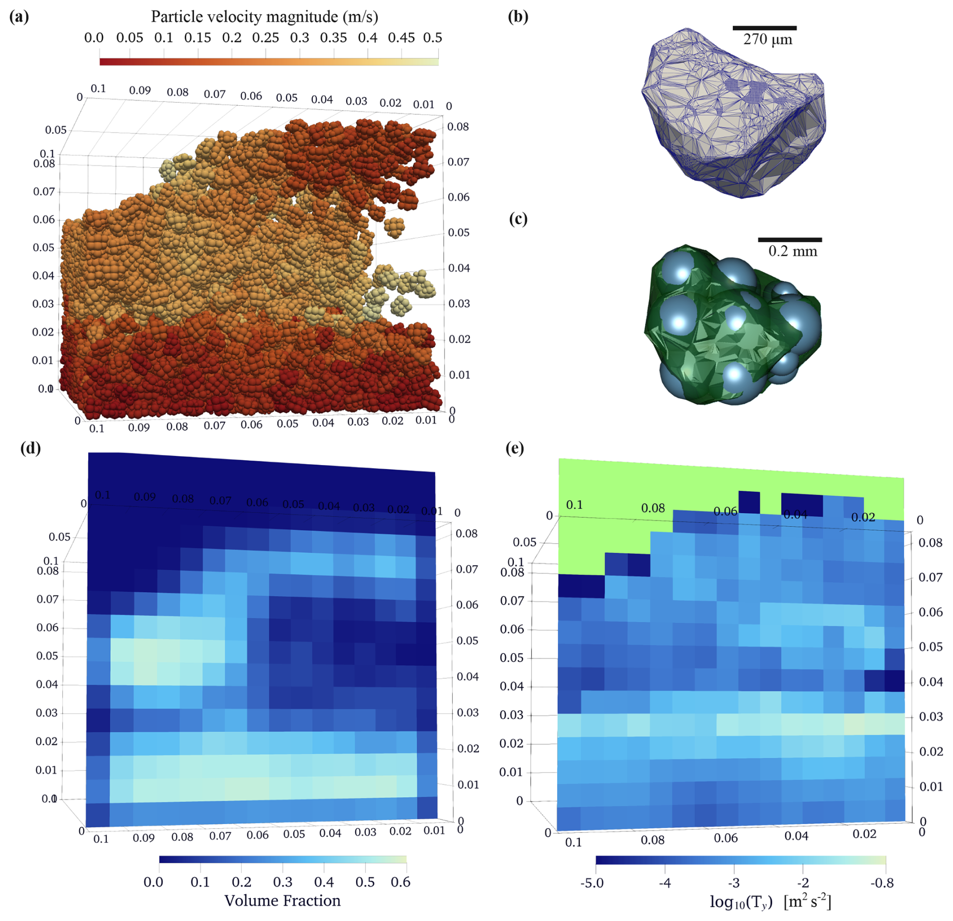
Figure 15 DEM simulation of a granular bed, fluidised with a gas velocity of 2 m s⁻¹, using glued-sphere particles (a). Reconstructed ash particle shape from Gabellini et al. (2025) (b), to which the glued-sphere particles in (a) are approximated, as shown in (c). Coarse-grained fields of the volume fraction (d) and vertical granular temperature (e) corresponding to the simulation time step shown in (a). Note that the pale green colour in (e) indicates NaN. This occurs at locations where T_y is set to 0 m² s⁻² by convention (see Appendix C2). Consequently, log₁₀(0) is undefined and is represented as NaN in ParaView.

To this end, we use the MFiX feature that approximates a glued-sphere particle to a target shape supplied in stereolithographic (STL) format to simulate a fluidised granular bed of volcanic ash particles (Fig. 15). The GSP geometry is fitted to that of an ash particle, obtained from the X-ray micro-tomography by Gabellini et al. (2025), and scaled up to reduce computational cost (Fig. 15b–c). The granular bed is fluidised through a basal inlet at 2 m s⁻¹, generating large bubbles that rise through the bed, as visible in the volume fraction field (Fig. 15d). The transition between dense and collisional flow regimes is reflected in a gradient in the vertical granular temperature (Fig. 15e).

5.4 Future work

The ethos behind Pysammos is heavily weighted by the idea of open-source code, well documented and structured to facilitate maintenance and future developments. The first version offers a range of advantageous features suitable for different types of users, nevertheless, there are aspects that can be further developed. Below we outline several implementations that would enhance the functionalities of this code package.

In order to work towards standardising and streamlining DEM post-processing software, future versions of this code package should incorporate data reading modules that are compatible with data from other DEM software, such as LAMMPS (available in the next release) or YADE, to fit the array structure that is used in the core functions. The current architecture is already designed to host new data readers. Regarding meshing, at present Pysammos offers a structured cuboid grid, a choice that is not optimal for all spatial model configurations. Greater flexibility in the meshing scheme would enable better alignment with complex geometries and minimise unnecessary sampling. Finally, the coarse-grained fields implemented in Pysammos are not taking into account the effect of hard boundaries as described in Weinhart et al. (2012), as it modifies the contact stress tensor. Therefore, future versions of this code should implement the calculation of the contact stress tensor for those particles in direct contact with the walls of a DEM model.

6 Conclusions

Granular flows, widespread in both natural systems and industrial applications, remain challenging to understand due to their highly complex particle–particle and particle–fluid interactions. DEM–CFD approaches provide detailed particle-scale information, but extracting relevant macroscopic continuum fields requires robust coarse-graining methodologies. In this work, we present Pysammos, a user-friendly, open-source Python package designed to streamline the coarse-graining of DEM data generated with MFiX and visualisation of results. The workflow enables flexible variable selection, mesh parametrisation, and phase-specific analysis of polydisperse mixtures of any particle shape. It produces vtkhdf outputs readily compatible with ParaView, as well as generic h5 files for further analysis. Its favourable algorithmic complexity allows it to run on standard computers or HPC systems with minimal computational overhead. We also demonstrate several key functionalities and exemplar applications, and provide guidance on best practices to ensure robust and reliable use of the code.

Appendix A: Input File Information

This appendix describes the input files required by Pysammos. As indicated in Fig. 1, these consist of a plain text configuration file, a particle properties file and a particle contacts file.

Listing A1 shows the configuration file format. For further details, visit the online documentation at https://claudia-elijas.github.io/pysammos/ (last access: 1 October 2026). The file is organised into sections, each marked by a header in square brackets, as described below.

The paths section specifies the path to the input files, for the particle properties and the particle contacts, and the path to the output directory. The timesteps section defines the time range of the CG analysis: t0 and tf are the first and last time steps, and td is the DEM file interval. The smoothing_function section specifies the weighting function for the CG, which may be Lucy, Gaussian, or HeavySide. The grid_info and fields_to_export sections control the CG meshing parameters and the set of continuum fields written to disk, respectively. The output_options section specifies the output format.

The key_mapping section maps the DEM simulation data fields to the keys expected by the source code in Pysammos. The required particle data consists of: particle ID, velocity, diameter (or radius), density, volume, mass, and optionally coordination number. The required contact data consists of: particle IDs of the two particles involved in each recorded collision, force acting on the first particle, and contact point (optional).

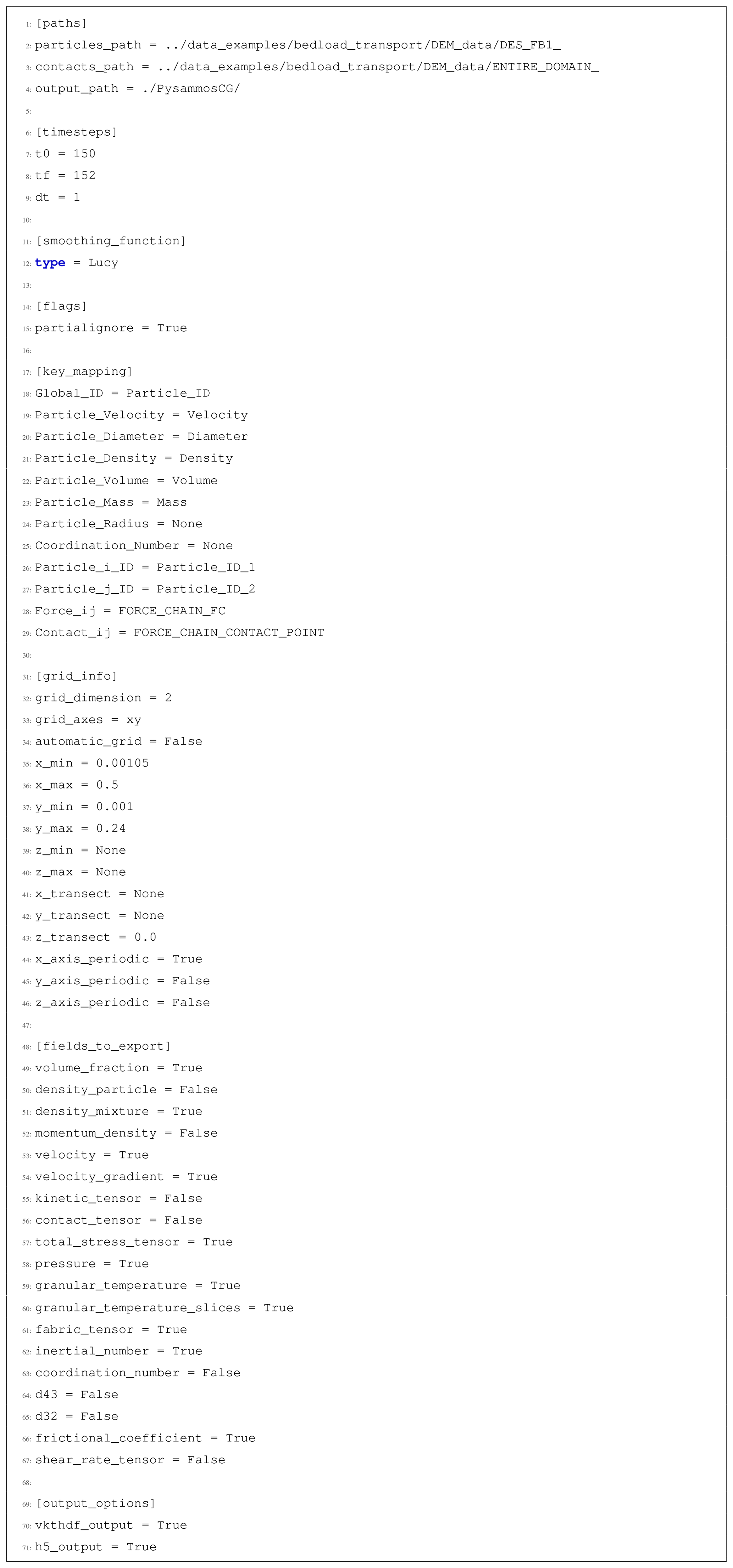
Listing A1 Configuration file for the bedload transport example provided in the online documentation.

Appendix B: Algorithms

This appendix contains the description of specific algorithms used in the core code.

B1 KMeans algorithm

The phase detection is carried out by clustering particle data with Python's KMeans (Pedregosa et al., 2011). The k-means algorithm, also referred to as Lloyd's algorithm (MacQueen, 1967; Lloyd, 1982), consists of the following steps: given a set X of N samples, it assigns an initial set C of K clusters and allocates each sample to its nearest cluster; subsequently, it generates new centroids (i.e., mean μ_j of the samples previously assigned to it); takes the difference between the previous and updated centroids and iterates until this difference stabilises, or similarly, inertia or the within-cluster sum-of-squares is minimised (Eq. B1).

$$\begin{array}{}\text{(B1)}& \sum _{i=\mathrm{1}}^N\underset{{\mathit{\mu }}_j\in C}{min}\left(\right||X_i-{\mathit{\mu }}_j|\left|\right)\end{array}$$

Nevertheless this method assumes the clusters are convex and isotropic, resulting in a lower accuracy when applied to elongated clusters. Further, Eq. (B1) does not represent a normalised metric, hence it is best used in relative terms within the same scaled dataset and should be used in conjunction with other metrics to decide the optimal number of clusters. For instance, the silhouette analysis calculates the distance from each point in one cluster to the neighbouring clusters and thus provides a more robust approach to assess the optimum number of clusters K that fit the dataset X.

B2 K-d tree search algorithm

The particle search within a finite volume around a grid point is carried out with Python scipy.spatial's cKDTree class, which implements the k-d tree form of nearest neighbour search to find all points within a radius of a query (Virtanen et al., 2020).

A k-d tree is a data structure built from recursively bisecting the search space in every dimension and collecting the coordinates of those splitting planes (Fig. B1). In three dimensions, the space is first bisected through the median of the data along the x-axis, and subsequently divided along the y-axis and finally, along the z-axis (Fig. B1b). This procedure is recursively applied until the tree is built. Then, the search begins at the root and descends through the levels of the tree (Fig. B1a). The branches are chosen based on the proximity of the query value to either of the split planes. This process is repeated alternating dimensions at each level until the subregions between splitting planes get sufficiently small. All points within a given radius from the query point are recorded.

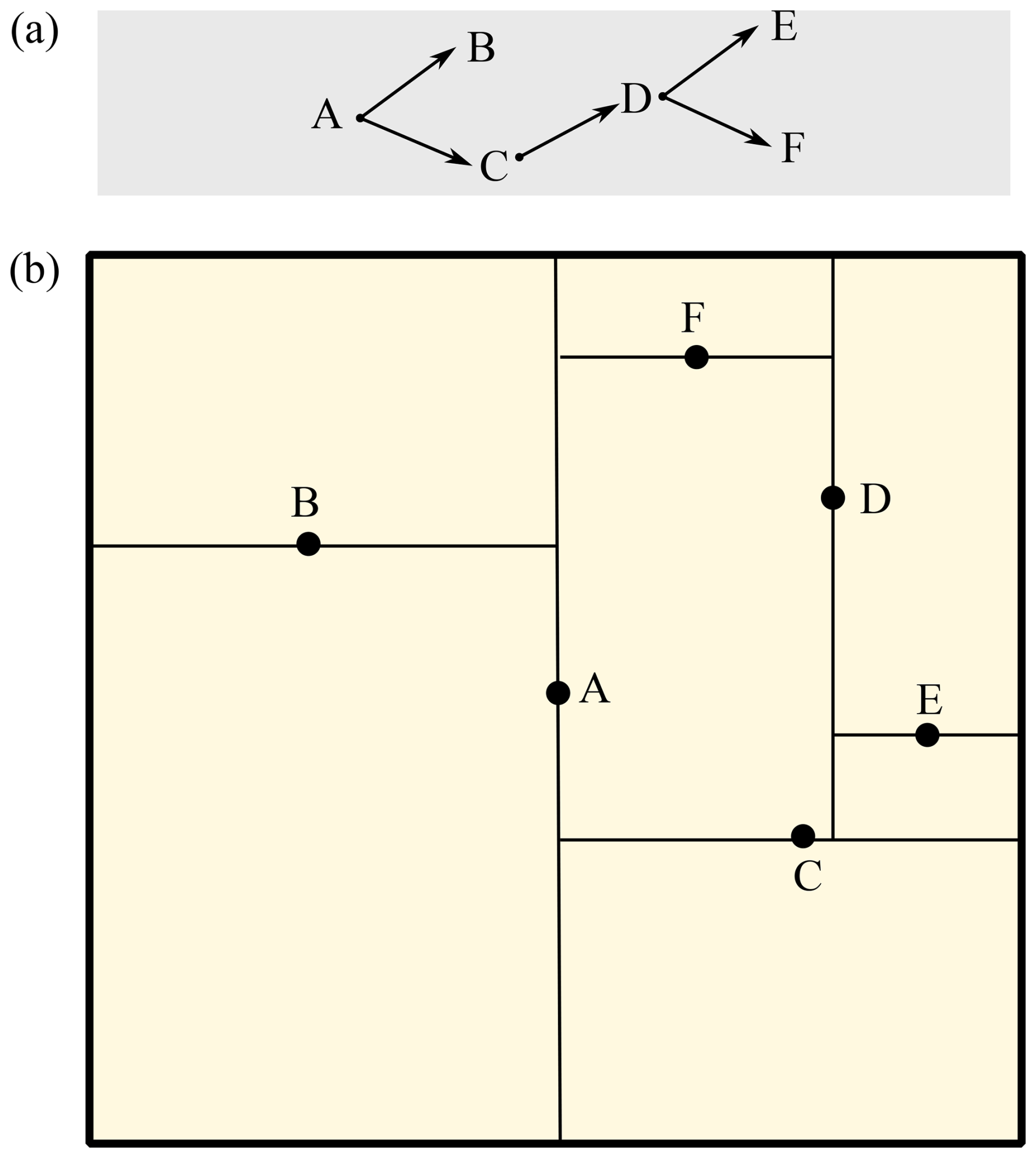
Figure B1 Simplified example of a k-d-tree in 2D (a) corresponding to the divisions in space shown in (b). Each level of the tree corresponds to a labelled line in the spatial visualisation. The levels of the tree alternate in axes (e.g., A is vertical, B and C are horizontal). Note that only a single branch is built completely, while others stop in earlier levels.

Opposite branches are also visited if the splitting plane lies within the search radius of the query point. The construction of the tree shows a computational complexity of O(Nlog N), and the search of the tree, O(log N) (Skrodzki, 2019).

B3 Lookup table algorithm

To speed up repeated evaluations of the CG weights for particle-grid point pairs, we implemented a lookup table algorithm (Fateman, 1989). This method discretises the input domain, and subsequently, evaluates the target function at those discrete points. The discretised points and their corresponding values yielded by the function are stored in a lookup table, with a corresponding index. Next, the continuous query values are mapped to the discrete index of the lookup table by dividing by the step size and rounding down.

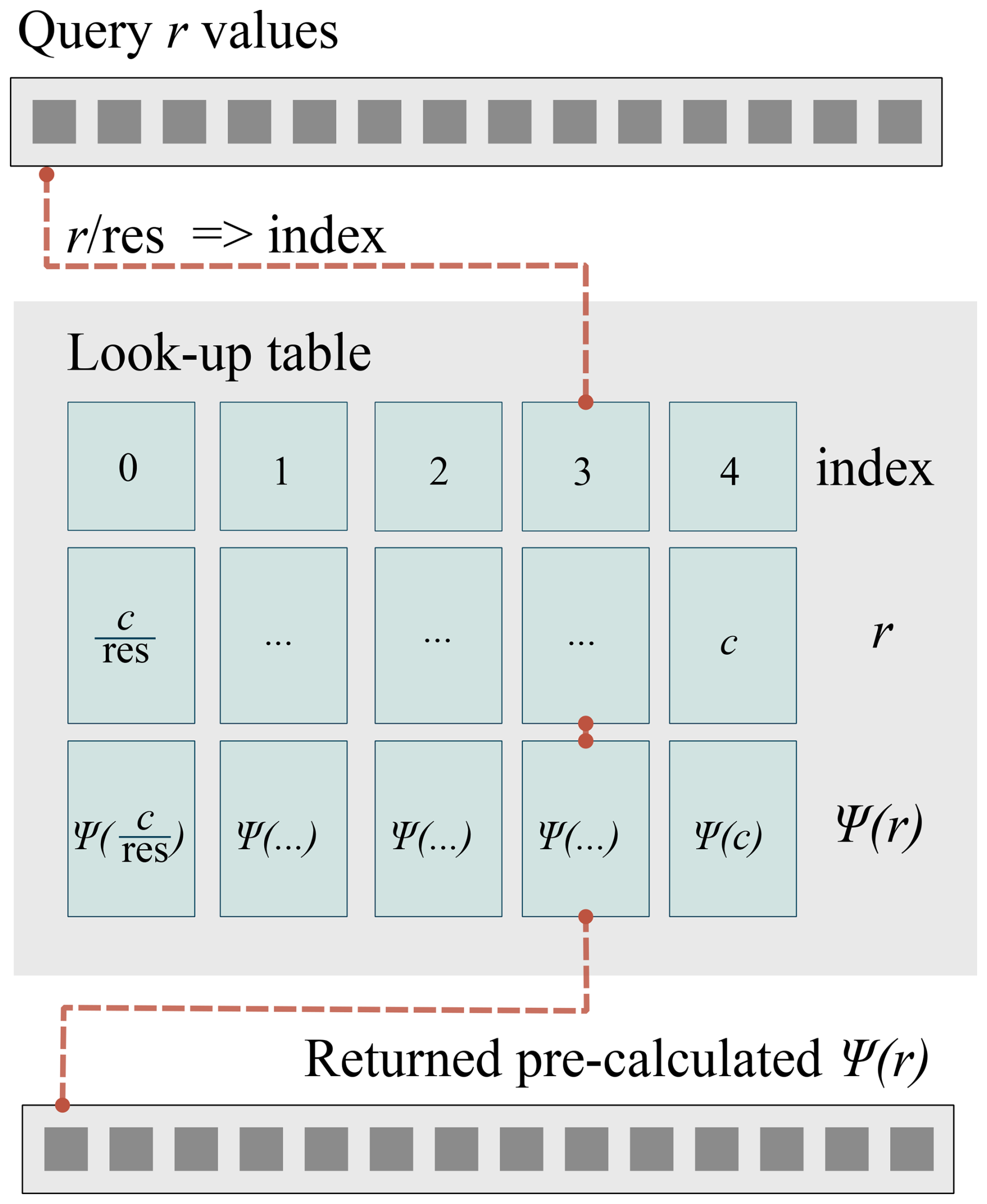
Figure B2 Schematic diagram of the lookup table algorithm implemented in Pysammos. r corresponds to the distance between a particle and a grid point. The resolution of the lookup table is res. Ψ(r) is the coarse-graining function, and c corresponds to its cut-off distance (i.e., Ψ(c)=0).

In Pysammos, the input domain consists of distances up to the cut-off distance, the target function is the CG weighting function, and the query values are the distances between grid points and particles near each grid point (Fig. B2). The application of a lookup table algorithm to CG weight calculation is particularly advantageous because the amount of particles that could physically be within a usual CG volume is finite, and therefore it scales well as the number of particles and grid points increases. Therefore, this approach avoids redundant computation, achieving the efficient retrieval of CG weights.

Appendix C: Continuum fields

This appendix details the calculation of the continuum fields output by Pysammos, in addition to those described in Sect. 2.

C1 Fundamental fields

The most fundamental CG fields are presented below, from which additional fields may be derived (Appendix C2). The macroscopic volume fraction, ϕ, is given by Eq. (C1):

$$\begin{array}{}\text{(C1)}& \mathit{\varphi }(\mathit{r},t)=\sum _{i=\mathrm{1}}^N{\mathit{\nu }}_i\mathrm{\Psi }(\mathit{r}-{\mathit{r}}_i(t\left)\right),\end{array}$$

where ν_i is the volume of particle i.

The macroscopic velocity field, V, is defined as the ratio between the momentum density vector, p (Eq. C2), and the mass density fields (Eq. 2), as shown in Eq. (C3).

$$\begin{array}{}\text{(C2)}& \mathit{p}(\mathit{r},t)=\sum _{i=\mathrm{1}}^N{m}_i{\mathit{v}}_i\mathrm{\Psi }(\mathit{r}-{\mathit{r}}_i(t\left)\right),\end{array}$$

where v_i is particle velocity.

$$\begin{array}{}\text{(C3)}& \mathit{V}(\mathit{r},t)={\displaystyle \frac{\mathit{p}(\mathit{r},t)}{\mathit{\rho }(\mathit{r},t)}}\end{array}$$

The fabric tensor (Eq. C4) describes the contact orientation distribution (Weinhart et al., 2013).

$$\begin{array}{}\text{(C4)}& \begin{array}{rl}\mathbf{F}(\mathit{r},t)& =\sum _{i=\mathrm{1}}^N\sum _{j=i+\mathrm{1}}^N\sum _{k=\mathrm{1}}^{C_{ij}}{\mathit{\nu }}_i{\mathit{n}}_{ij}^k\otimes {\mathit{n}}_{ij}^k\\ & \underset{\mathrm{0}}{\overset{\mathrm{1}}{\int }}\mathrm{\Psi }(\mathit{r}-{\mathit{r}}_i+s{\mathit{a}}_{ij}^k)\mathrm{d}s,\end{array}\end{array}$$

where ${\mathit{n}}_{ij}^k$ is the contact normal unit vector.

C2 Secondary fields

The continuum fields, derived from fundamental fields, calculated in Pysammos are presented below.

The area-weighted and volume-weighted average diameter are calculated according to Eqs. (C5) and (C6), respectively.The coarse-grained coordination number Z is given by Eq. (C7).

$$\begin{array}{}\text{(C5)}& {\displaystyle }d\mathrm{32}(\mathit{r},t):={\displaystyle \frac{\sum d_i^{\mathrm{3}}\mathrm{\Psi }(\mathit{r}-{\mathit{r}}_i(t\left)\right)}{\sum d_i^{\mathrm{2}}\mathrm{\Psi }(\mathit{r}-{\mathit{r}}_i(t\left)\right)}}\text{(C6)}& {\displaystyle }d\mathrm{43}(\mathit{r},t):={\displaystyle \frac{\sum d_i^{\mathrm{4}}\mathrm{\Psi }(\mathit{r}-{\mathit{r}}_i(t\left)\right)}{\sum d_i^{\mathrm{3}}\mathrm{\Psi }(\mathit{r}-{\mathit{r}}_i(t\left)\right)}}\text{(C7)}& {\displaystyle }Z(\mathit{r},t):={\displaystyle \frac{\sum z_i\mathrm{\Psi }(\mathit{r}-{\mathit{r}}_i(t\left)\right)}{\sum \mathrm{\Psi }(\mathit{r}-{\mathit{r}}_i(t\left)\right)}}\end{array}$$

where z_i is the coordination number of a particle i and describes the number of contacts a given particle is involved in. The averaged particle density ρ_p results from the ratio between the mixture density and the volume fraction (Eq. C8).

$$\begin{array}{}\text{(C8)}& {\mathit{\rho }}_{\mathrm{p}}(\mathit{r},t)={\displaystyle \frac{\mathit{\rho }(\mathit{r},t)}{\mathit{\varphi }(\mathit{r},t)}}\end{array}$$

The gradient of the velocity ∇V computed in Pysammos corresponds to the velocity of the granular mixture, even when partial fields are requested.

∇V is used to carry out a linear interpolation of the coarse-grained velocity at a grid point, V(r,t), to the position of a particle i, V(r_i(t),t), in order to obtain an accurate estimate of the local particle velocity fluctuations, ${\mathit{V}}_i^{*}$ (Eq. 7), with respect to the computed macroscopic field.

$$\begin{array}{}\text{(C9)}& \mathit{V}\left({\mathit{r}}_i\right(t),t):=\mathit{V}(\mathit{r},t)-\mathrm{\nabla }\mathit{V}(\mathit{r},t)\cdot (\mathit{r}-{\mathit{r}}_i)\end{array}$$

Note that the negative sign arises from defining the displacement vector as (r−r_i) i.e. directed from the particle position to the grid point, rather than (r_i−r). This convention is adopted for consistency with the preceding coarse-grained fields formulations.

In Pysammos we offer two different ways of computing the velocity gradient. The first uses finite difference (Eq. C10). For robustness, the components of ∇V match the geometry of the grid, that is, the gradient is only computed for the planes along which grid points have been generated.

$$\begin{array}{}\text{(C10)}& \mathrm{\nabla }\mathit{V}(\mathit{r},t)=\left[\begin{array}{ccc}\frac{\partial u}{\partial x}& \frac{\partial u}{\partial y}& \frac{\partial u}{\partial z}\\ \frac{\partial v}{\partial x}& \frac{\partial v}{\partial y}& \frac{\partial v}{\partial z}\\ \frac{\partial w}{\partial x}& \frac{\partial w}{\partial y}& \frac{\partial w}{\partial z}\end{array}\right]\end{array}$$

where u, v and w are components of the coarse-grained velocity of the granular mixture v in the x, y and z axes, respectively, and $\mathit{r}=\left[\begin{array}{c}x,y,z\end{array}\right]$.

The second computes a kernel-consistent gradient of V(r,t) (Eq. C3), that best describes the averaged particle velocities around the kernel. The gradient is calculated as G=∇V by minimising the weighted square error, ε(G) (Eq. C11) according to least-squares linear fit, where Ψ(r−r_i(t)) is written as Ψ for simplicity.

$$\begin{array}{}\text{(C11)}& \mathit{\epsilon }\left(\mathbf{G}\right(\mathit{r}\left)\right)=\sum _i\mathrm{\Psi }{m}_i|{\mathit{v}}_i-\mathit{V}(\mathit{r},t)+\mathbf{G}(\mathit{r}{)}_i\cdot (\mathit{r}-{\mathit{r}}_i){|}^{\mathrm{2}}\end{array}$$

Solving the minimisation we obtain that G(r) is given by Eq. (C12).

$$\begin{array}{}\text{(C12)}& \begin{array}{rl}\mathbf{G}\left(\mathit{r}\right)& ={\left(\sum _i\mathrm{\Psi }{m}_i(\mathit{r}-{\mathit{r}}_i)\otimes (\mathit{r}-{\mathit{r}}_i)\right)}^{-\mathrm{1}}\\ & \left(\sum _i\mathrm{\Psi }{m}_i({\mathit{v}}_i-\mathit{V}(\mathit{r},t\left)\right)\otimes (\mathit{r}-{\mathit{r}}_i)\right)\end{array}\end{array}$$

Granular temperature, T, measures the level of fluctuation of particle velocity about the macroscopic velocity of the granular mixture (Goldhirsch, 2008). It is calculated as a spatial average of the squared velocity fluctuations; squaring is necessary because, by definition, the average of the (non-squared) fluctuation velocity is zero, so squaring avoids cancellation between fluctuations of equal magnitude but opposite sign,

$$\begin{array}{}\text{(C13)}& T(\mathit{r},t):={\displaystyle \frac{\mathrm{1}}{D\mathit{\rho }(\mathit{r},t)}}\text{tr}\left({\mathit{\sigma }}^{k\prime }\right(\mathit{r},t\left)\right),\end{array}$$

where D is the number of spatial dimensions considered. Note that the scale-independent term of the kinetic tensor must be used (σ^k ′), as T focuses on the local velocity fluctuations, ${\mathit{V}}_i^{*}$ (Eqs. 6 and 7). It is important to note that in regions with no particle influence (i.e., $\mathit{\rho }(\mathit{r},t)=\mathrm{0}$), T is set to zero, to avoid the undefined division of 0 by 0, and subsequent NaN propagation. Although a NaN would be more mathematically accurate, we have opted for this common numerical-safety practice.

Pysammos also offers the computation of granular temperature following two different averaging methods by slices, and are exported separately by request, given their different structure (Plimpton, 1995; Zhang and Kamrin, 2017). The source code for these alternative methods can be found in the sub-package macroscopic_fields.sliced.

∇V is also used to evaluate the shear rate tensor Γ, which describes the deformation of a granular mixture due to velocity gradients (Eq. C14).

$$\begin{array}{}\text{(C14)}& \mathbf{\Gamma }(\mathit{r},t):={\displaystyle \frac{\mathrm{1}}{\mathrm{2}}}\left(\mathrm{\nabla }\mathit{V}\right(\mathit{r},t)+\mathrm{\nabla }\mathit{V}(\mathit{r},t{)}^T)\end{array}$$

Deviatoric stress provides information about the anisotropic stresses (i.e., not hydrostatic) due to stress loading. We obtain any stress deviator, Π_D, as shown in Eq. (C15).

$$\begin{array}{}\text{(C15)}& {\mathbf{\Pi }}_{\mathrm{D}}(\mathit{r},t):=\mathbf{\Pi }(\mathit{r},t)-{\displaystyle \frac{\mathrm{1}}{D}}\text{tr}\left(\mathbf{\Pi }\right(\mathit{r},t\left)\right)\mathbf{I}\end{array}$$

where Π is any tensor and I is the identity matrix. The magnitude of any of the computed tensors (e.g., σ^c, σ^k, σ, Γ, σ_D) is obtained by calculating the second invariant of the tensor, J₂, shown in Eq. (C16).

$$\begin{array}{}\text{(C16)}& J_{\mathrm{2}}(\mathit{r},t):=\mathit{\alpha }\text{tr}\left({\mathbf{\Pi }}^{\mathrm{2}}(\mathit{r},t)\right),\text{where}\mathit{\alpha }=\left\{\begin{array}{ll}\frac{\mathrm{1}}{\mathrm{2}},& \text{if }\mathbf{\Pi }\ne \mathbf{\Gamma }\\ \mathrm{2},& \text{if }\mathbf{\Pi }=\mathbf{\Gamma }\end{array}\right.\end{array}$$

The second invariant of Γ is related to the effective shear rate ${\dot{\mathit{\gamma }}}_{\text{eff}}=\sqrt{\mathrm{2}{J}_{\mathrm{2}}}$, hence α=2 when Π=Γ. Pressure, p, corresponds to the hydrostatic components of σ (Eq. C17).

$$\begin{array}{}\text{(C17)}& p(\mathit{r},t):={\displaystyle \frac{\mathrm{1}}{D}}\text{tr}\left(\mathit{\sigma }\right(\mathit{r},t\left)\right)\end{array}$$

The coefficient of friction μ is also provided as shown in Eq. (C18).

$$\begin{array}{}\text{(C18)}& \mathit{\mu }(\mathit{r},t):={\displaystyle \frac{\left|\mathit{\sigma }\right(\mathit{r},t\left)\right|}{p(\mathit{r},t)}}\end{array}$$

A widely accepted rheological model for dense granular flows is the so-called μ(I)-rheology. It is a phenomenological model that applies to homogeneously sheared flows in the dense, quasi-static, and inertial flow regimes. The μ(I)-rheology presents a one-to-one relation between the friction coefficient (i.e. the shear-to-normal stress ratio, μ) and the inertial number, I (Eq. C19).

$$\begin{array}{}\text{(C19)}& I(\mathit{r},t):={\displaystyle \frac{\left|\mathbf{\Gamma }\right(\mathit{r},t\left)\right|\overline{d}}{\sqrt{p(\mathit{r},t)/{\mathit{\rho }}_{\mathrm{p}}(\mathit{r},t)}}},\end{array}$$

where $\overline{d}$ is the representative particle size (Sect. 3.4). The inertial number is a measure of the dynamic state of a granular medium. It is also understood as the ratio of (1) the microscopic timescale (or scale of rearrangement), representing the time a particle takes to fall into a slit of a given diameter under a given pressure; and (2) the macroscopic time scale, linked to the average deformation (GDR MiDi, 2004).

Some of the implementations above are returned alongside possible variations. For instance, pressure is returned in 1D, 2D, and 3D. The stress tensors are provided in 2D and 3D, with their respective second invariants and deviatoric tensors. Granular temperature is also returned in 1D and 3D. The coefficient of friction is calculated with the deviatoric stress, and in 1D, 2D and 3D. The inertial number is also computed with the deviatoric shear stress , with different components of pressure, and different measures of characteristic grain size.

Appendix D: Data mapping structures

This appendix outlines the data structures and mapping strategies used to link different data representations within the code.

D1 Mapping particles

The function data_handle.contacts.particle_mapper.map_contact_data() maps the contact data (particle interaction pairs and force) to the particle data (position and diameter), so that the branch vectors of particle interactions can be calculated. On the one hand, the particle data consists of the following arrays: particle ID, and particle diameter, mass, velocity and position. On the other hand, contact data consists of the following arrays: particle ID of the particles upon which the contact force is exerted (particles A), the force acting on particles A, and particle ID of the particles in contact with particles A (particles B). The arrays containing the contact data are concatenated such that both perspectives of the interaction are accounted for in a single array (i.e., $A_{\mathrm{con}}=\mathit{\{}\mathrm{particles}A,\mathrm{particles}B\mathit{\}}$ and B_con={particles B, particles A}). That way, Eq. (5) can be applied directly to contact data (Fig. D1b). Hence, the contact-to-particle data mapping involves the association of each element of A_con (and B_con) with the corresponding element in particle ID array of the particle data (grey array in Fig. D1a).

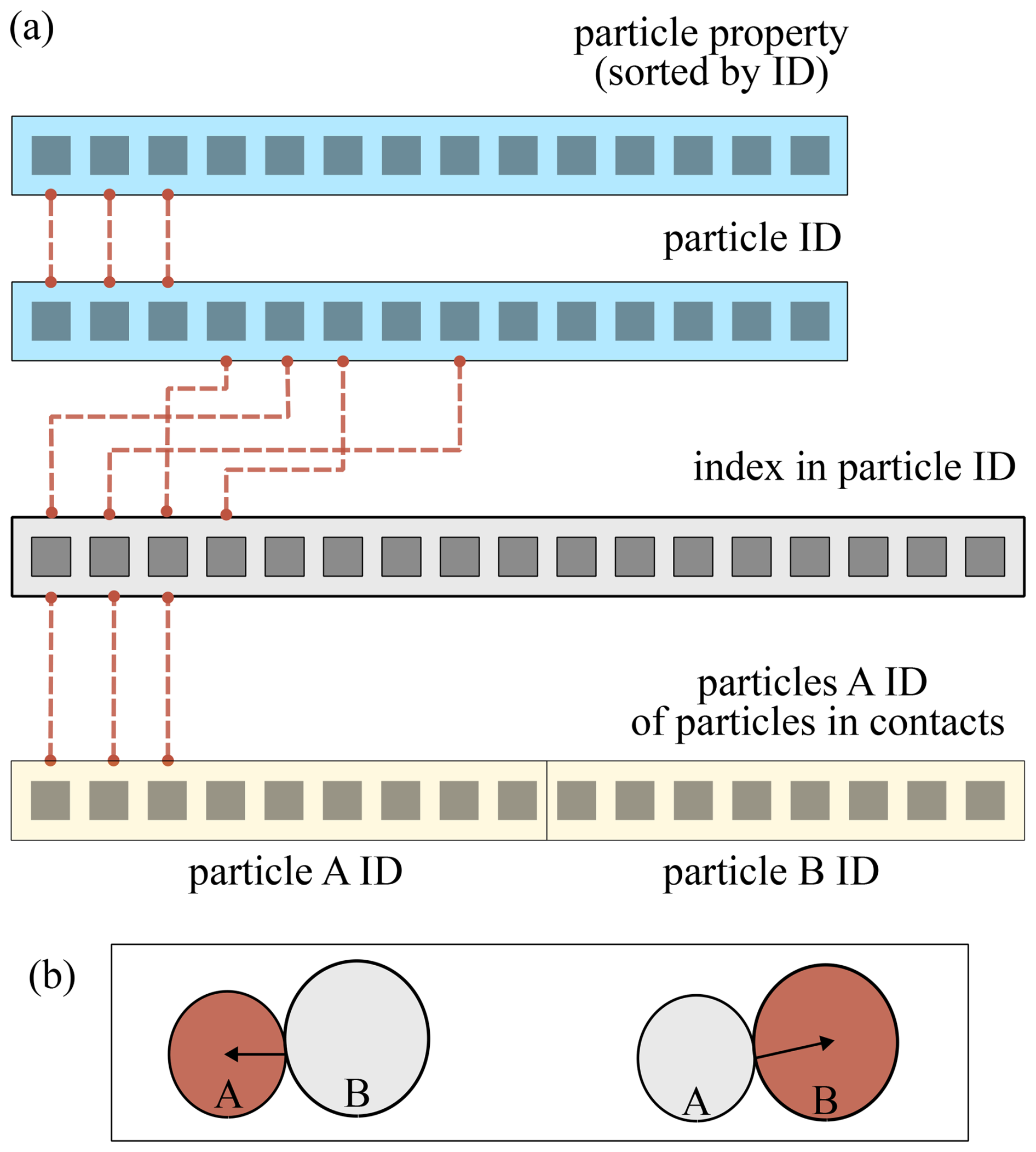
Figure D1 Conceptual diagram illustrating the relationship between the particle data (blue arrays) and contact data (yellow arrays) through the index mapping (grey) array. The grey array maps the indices of the contact data to the particle data, which is sorted by particle ID. The contact data has previously been arranged such that both sides of the interaction are taken into account in a single array, i.e., the effect on particle A, and on particle B (b).

D2 Correcting for periodic boundaries

The module data_handle.contacts.complete.branch_vectors provides functions to calculate the branch vectors from contact points to particle centres (from_contacts) or from particle diameters to particle centres (from_diameters), in case the contact point is not provided. Both functions handle periodic boundary corrections along each axis using the Minimum Image Convention (MIC), by which displacements are calculated to the nearest periodic equivalent as shown in Eq. (D1) (Gorbunov et al., 2022).

$$\begin{array}{}\text{(D1)}& \mathrm{\Delta }{r}_i^{\mathrm{c}}=(r_i^A-r_i^B)-L_i\lfloor {\displaystyle \frac{r_i^A-r_i^B}{L_i}}\rceil ,i\in \mathit{\{}x,y,z\mathit{\}},\end{array}$$

where $\mathrm{\Delta }{r}_i^{\mathrm{c}}$ is the corrected displacement between particles A and B in a given dimension, $r_i^A-r_i^B$ is the uncorrected displacement between the two particles in a given dimension and L_i is the length of the box in a given dimension. The application of the MIC to a two-dimensional scenario is illustrated in Fig. D2.

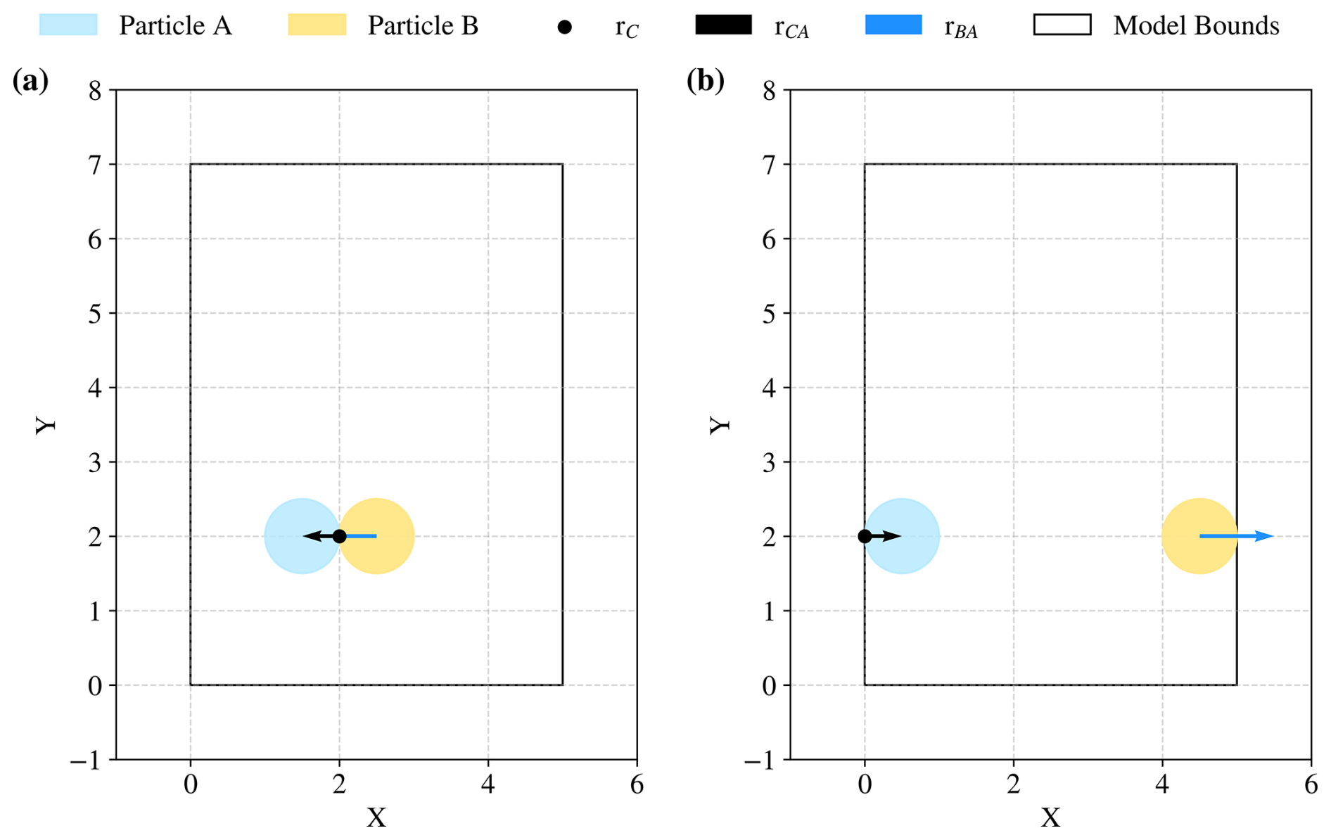
Figure D2 Two-dimensional illustration of the application of the Minimum Image Convention (MIC) for particle pairs located well within the model domain (a) and interacting across periodic boundaries (b). In case (b), displacement vectors are computed using the nearest periodic image, following Eq. (D1). All particles have identical radius (R=0.5). The contact point, r_C, is defined on particle A (purple) and is depicted with a black point. The branch vector from the contact point to the centre of particle A, r_CA, is shown by the black arrow, while the vector from the centre of particle B (red) to the centre of particle A, r_BA, is indicated by the blue arrow. The boundaries of the model domain are delineated by the black box.

D3 Deletion of duplicates

The module data_handle.contacts.quality_check.duplicates provides the tools to check for duplicate particle contacts in the contact data files, and delete them if present. Duplicate particle contacts often correspond to ghost particles near CPU region bounds used in parallel DEM computations. Ghost particles may be written by several CPUs, generating duplicate contacts in the output files. If this artefact is not addressed, the CG measures that rely on contact forces or branch vectors could be somewhat skewed.

In the function data_handle.contacts.quality_check.duplicates.get_unique_pairs() we sort the array of particles A and particles B involved in contact, ensuring that $(A,B)=(B,A)$ (Eq. D2), and record the indices of the unique pairs. Any non-unique pairs are deleted with the function data_handle.contacts.quality_check.duplicates.delete().

$$\begin{array}{}\text{(D2)}& p_k=\left(\text{min}(a_k,b_k),\text{max}(a_k,b_k)\right),k=\mathrm{1},\mathrm{\dots },N,\end{array}$$

where p_k is the kth particle pair, a_k and b_k are the IDs of the particles involved in the kth contact, and N is the total number of recorded particle pairs.

D4 Particle-node association

The particle-node association data are exported by the k-d tree algorithm as two arrays (Appendix B2). The first array contains the indices of particle data arrays (Fig. D3a, e.g., position), for each particle at each grid point in sequential order (Fig. D3b). The second array contains the offsets into the first array, providing the starting index of the particles associated with a given grid point (Fig. D3c). Note that this relation is correct given that the particle data arrays are sorted by particle ID just after being read.

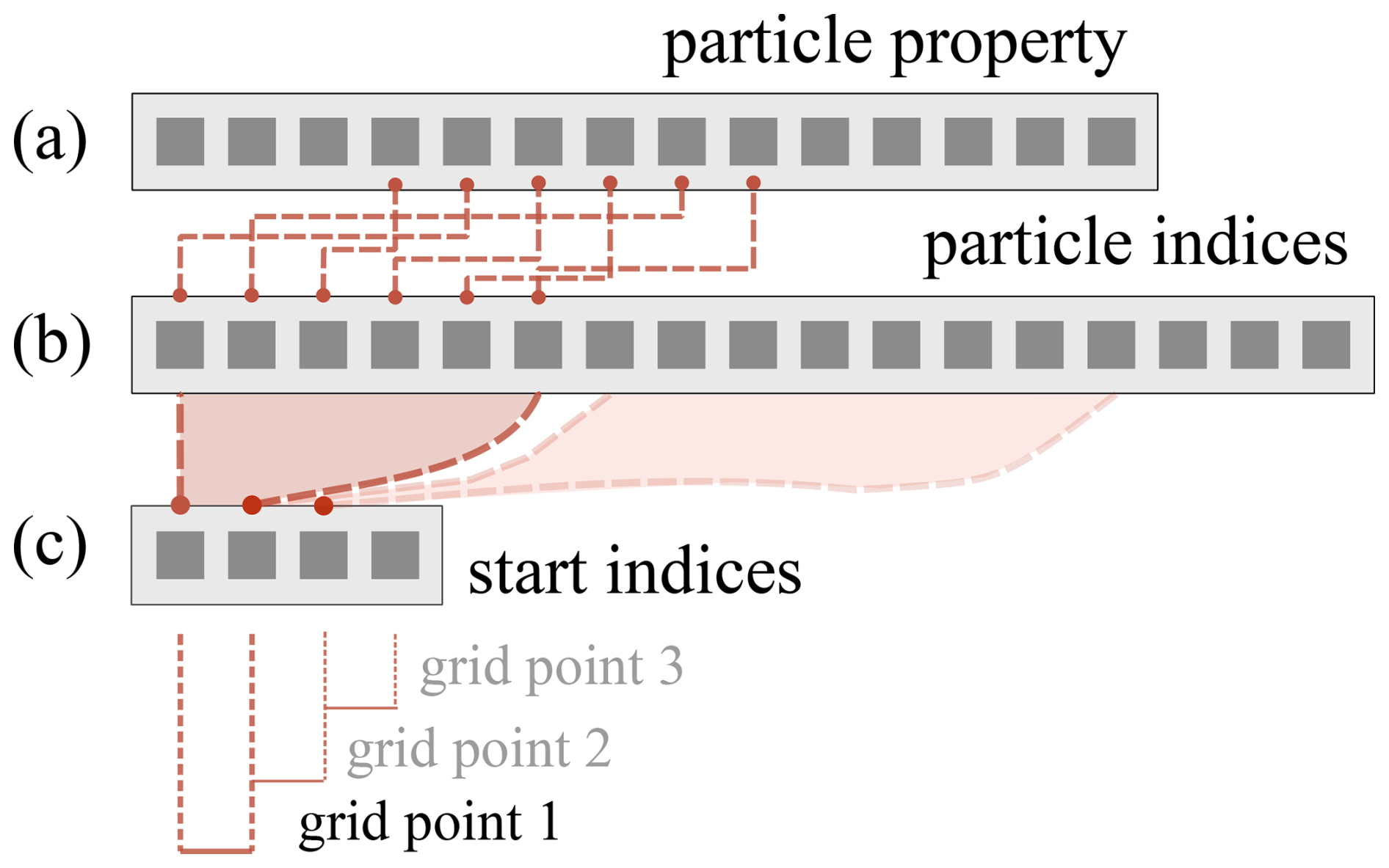
Figure D3 Schematic representation of the relation between the particle properties arrays (a) and the arrays exported by the function neighbour_search.grid_particle_search.particle_node_match: the particle indices array (b), containing the indices of particle properties arrays in sequential order for each particle at each grid point; and the start indices array (c), providing the starting index of the particles associated with a given grid point. This relation is correct given that the arrays containing particle properties are sorted by particle ID.

Empty grid points (i.e., those with no particles within the cut-off radius) are handled by appearing as zero-length slices in the second array, thus ensuring both efficiency and robustness. This structure is employed because it only uses arrays. The use of lists of arrays with variable lengths is avoided, as it is more computationally costly to check the type and size of each element of the list.

Appendix E: Optimisation strategies

This appendix outlines the structural design choices in Pysammos. The computational cost of the code is dominated by data handling rather than individual numerical operations. The scalability of the execution gives rise to bottlenecks that limit the efficiency by memory bandwidth rather than raw CPU performance. Code performance was enhanced by tackling bottlenecks identified in the resource usage analysis, employing algorithmic optimisation or the Numba Python compiler. Each bottleneck was addressed with a unique strategy that suited that particular operation, specified below:

1. Reading and writing data. Large portions of memory are required to load and write single data files meaning that it is an operation that should be done in succession. This was accommodated by an architecture that loops over time steps and optimises the operations within each time step.

2. Particle to grid point association. There are many ways to perform proximity searches with ranging scalability complexity. We applied the k-d tree algorithm (Skrodzki, 2019), a space partitioning proximity search with runtime O(log N), as opposed to the linear search with complexity O(dN), where d and N are the dimensionality and number of elements of the system (Appendix B2).

3. Particle to grid point weighting. The re-computation of CG weighting functions, in particular the Gaussian, is increasingly inefficient as the number of particles and grid points grows. Lookup tables of precomputed weights reduce the number of times these weights are actually calculated, and thus increase the efficiency of this operation (Appendix B3).

4. Weighted average computation at all grid points. In the presence of a large number of grid points, the runtime of this calculation grows linearly with time if done in loops or requires too much memory if approached with vectorisation. Hence, this operation could benefit from Numba acceleration and parallel computing, given that it is completely independent from one grid point to another (Appendix E1).

E1 Numba compilation

Numba is an open-source just-in-time (JIT) compiler for Python (Lam et al., 2015). It translates functions marked with the JIT decorator into (faster) machine code, using Low Level Virtual Machine (LLVM), and caches it until execution. Once Numba has identified the functions to translate, it determines the data types of the function arguments prior to runtime to avoid overhead, as is the case of Python's dynamic typing approach. Numba supports NumPy library objects and operations, making it an invaluable tool for scientific computing and data analysis.

Numba also offers the possibility to compute loops in parallel. This option allows CPU multi-threading, where each thread executes a chunk of the loop independently and combines the results at the end. Numba may additionally vectorise inner loops within a parallelised task using single instruction multiple data (SIMD) operations. The parallelisation option offered by Numba requires the user to ensure the robustness of the parallelised loop, that is, there are no cross-iteration dependencies.

In Pysammos, the capabilities of Numba that reduce Python-level overhead were leveraged in operations that involved the totality of grid points and particles, like the calculation of continuum fields (bottleneck 4). The parallelisation option was implemented as well, however, the nature of the problem, i.e., memory-bandwidth bound, meant that computation did not overly benefit from parallelisation.