The one-Layer Antarctic model for Dynamical Downscaling of Ice–ocean Exchanges (LADDIE) version 2.0

Projections of Antarctic mass loss and its contribution to sea-level rise are highly sensitive to the applied ocean-driven melting. As fully coupled continental-scale ocean–ice sheet models are scarce, ice sheet models are typically run in standalone configurations, forced with parameterised sub-shelf melting. To provide a physically more detailed alternative to melt parameterisations, we here present version 2.0 of the one-Layer Antarctic model for Dynamical Downscaling of Ice–ocean Exchanges (LADDIE). LADDIE is a two-dimensional model of the upper mixed layer below ice shelves and can reproduce observed spatial patterns in sub-shelf melting. Version 2.0 has improved computational performance due to parallellisation, discretisation on an unstructured mesh, and a more stable time stepping scheme. The model is fully integrated with the UFEMISM ice sheet model, allowing for coupled simulations on the same mesh. We evaluate the model by comparing it to LADDIE 1.0, showing that the simulated melt patterns are consistent across both model versions, whilst the computation time can be reduced by one order of magnitude due to parallellisation. The model is evaluated against an ensemble of 3D ocean models in both idealised and realistic pan-Antarctic domains at 2 km resolution. In both cases, LADDIE melt rates, melt patterns, and melt sensitivities are close to the multi-model mean. An evaluation against four pan-Antarctic satellite estimates, shows an overall good agreement in integrated melt rates per ice shelf, without the need for regional tuning. At a resolution of 120 m, LADDIE is able to reproduce the fine-scaled network of basal channels, observed on Pine Island ice shelf. Finally, we compare an idealised coupled UFEMISM–LADDIE simulation to a simulation with a quadratic melt parameterisation. The coupled simulation produces a threefold increase in grounding line retreat and volume above floatation loss. Based on these results, we conclude that LADDIE 2.0 can be a useful tool to simulate ice–ocean interactions in a computationally efficient way.

1 Introduction

Mass loss from the Antarctic ice sheet has accelerated over the past decades (Otosaka et al., 2023). This acceleration is dominated by the Amundsen Sea region in West-Antarctica, where ocean-driven melting causes ice shelf thinning (Paolo et al., 2015). Such ice shelf thinning reduces the capacity for ice shelves to buttress the flow of grounded ice towards the ocean, which contributes to sea-level rise (Reese et al., 2018b). Ensemble projections of Antarctic mass loss indicate that sub-shelf melting is a major source of discrepancy between ice sheet models, and therefore a primary source of uncertainty in assessing Antarctica's future contribution to sea-level rise (Seroussi et al., 2024; Beckmann et al., 2025).

The most realistic representation of sub-shelf melting requires fully coupled ice sheet–ocean models to account for a varying geometry. To accurately represent sub-shelf melting near the grounding line, McCormack et al. (2024) concluded that ocean models should have a resolution of 2 km or finer. A similar, or higher, resolution is required to resolve sub-shelf melting in basal channels (Alley et al., 2022; Lambert et al., 2023; Zhou et al., 2026). Such resolutions, however, put a heavy demand on 3D ocean models and are unfeasible for simulations over time scales relevant for ice sheets (multiple centennia). The resolution of coupled pan-Antarctic ice–ocean simulations is commonly at most 0.25°, which equates to 4–14 km below ice shelves (Smith et al., 2021; Siahaan et al., 2022; Pelletier et al., 2022; Sauerland et al., 2025). Using the benefits of an unstructured mesh, this resolution can be brought down to 2–10 km (Richter et al., 2025). However, at present, only for regional ice–ocean configurations are resoltions of 2 km or finer achieved Bett et al. (e.g., 2024); Goldberg and Holland (e.g., 2022); De Rydt and Naughten (e.g., 2024).

As a consequence of these technical challenges, most practical examples of Antarctic ice sheet projections are currently based on stand-alone ice sheet models with sub-shelf melt parameterisations (Seroussi et al., 2024). These parameterisations translate ocean temperatures outside ice shelf cavities to horizontal fields of melt rates at the base of ice shelves (Jourdain et al., 2020). A variety of parameterisations currently exist, with the most commonly used ones being a quadratic dependence on ocean temperatures (Favier et al., 2019), the box model PICO (Reese et al., 2018a), and a plume model (Lazeroms et al., 2018). These parameterisations all aim to represent an overturning circulation in ice shelf cavities which transports heat towards the ice–ocean interface, and meltwater produced by sub-shelf melting out of the cavities. However, a detailed comparison to 3D ocean models and observations illustrated that these parameterisations struggle to represent the horizontal pattern of sub-shelf melting (Burgard et al., 2022)

In an idealised framework, Berends et al. (2023) showed that the dynamic behaviour of ice sheet models is highly sensitive to this spatial melt pattern. In order to improve the spatial pattern of sub-shelf melting, we developed the one-Layer Antarctic Model for Dynamical Downscaling of Ice–ocean Exchanges (LADDIE 1.0, Lambert et al., 2023). This model is a two-dimensional extension of the plume model, resolving the impact of topographic steering and Coriolis deflection on the meltwater flow along the ice shelf base. Coupled to the ice sheet model IMAU-ICE (Berends et al., 2022) in an idealised setting, LADDIE 1.0 can induce a stronger dynamic ice sheet response to ocean warming than the most commonly used parameterisations (Jesse et al., 2025). In terms of practical use, however, LADDIE 1.0 can only be configured at pan-Antarctic scales at a coarse resolution due to computational limitations. This implies that the model cannot achieve substantially higher pan-Antarctic resolutions than 3D ocean models.

To overcome these computational limitations, we have developed a new model version, v2.0. The major changes since v1.0 are a translation from uncompiled Python to compiled Fortran code, and a translation from finite difference numerics on a square grid to finite volume numerics on an unstructured mesh. These changes were achieved using the Utrecht Polar SYstem (UPSY) toolbox as developed for the UFEMISM ice sheet model (Berends et al., 2025). Benefiting from this toolbox, LADDIE 2.0 can now be run in parallel. Finally, the new model is fully integrated with UFEMISM, allowing both models to run interactively on the same adaptive, dynamic mesh.

In this paper, we describe LADDIE 2.0, and evaluate its behaviour using a variety of use cases. In Sect. 2, we describe the model basics. In Sect. 3, we evaluate LADDIE 2.0 by comparing it to LADDIE 1.0, to 3D ocean models, and to satellite-derived estimates. In Sect. 4, we present results from an idealised coupled UFEMISM–LADDIE simulation and compare it to a UFEMISM simulation with parameterised sub-shelf melting. The paper ends with a Discussion (Sect. 5) and Conclusions.

2 Model description

For a full description of the LADDIE model, we refer to Lambert et al. (2023). Here, we summarise the model basics and any differences between v1.0 and v2.0.

2.1 General

LADDIE is a two-dimensional model, describing a quasi-horizontal slab of ocean directly below the ice shelf (Fig. 1). Vertically, it describes the upper mixed layer with variable thickness, making the model domain bounded between the ice shelf base and the base of the mixed layer. At the ice shelf base, the model simulates sub-shelf melting; at the mixed layer base, the model simulates entrainment of ambient waters from the cavity below. Laterally, the model domain is bounded between the grounding line and the calving front.

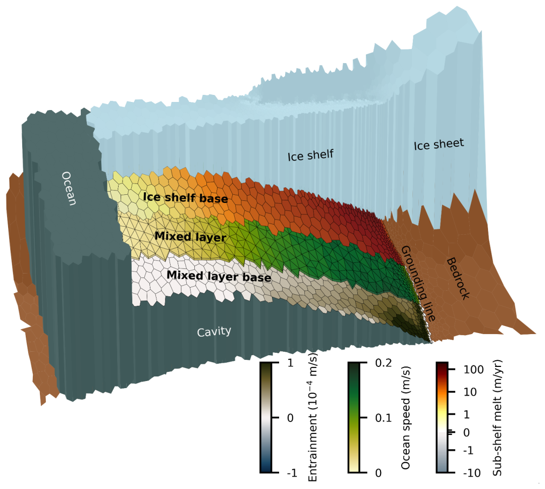
Figure 1 Schematic of main processes and their spatial discretisation: entrainment at the base of the mixed layer (voronoi cells), ocean currents within the mixed layer (trianglar prisms with finite thickness), and sub-shelf melting (voronoi cells) at the ice/ocean interface. This illustration is based on an ISOMIP+ simulation (Sect. 3.2.1) with resolutions ranging from 1 km near the grounding line to 4 km over the rest of the ice shelf.

Within the mixed layer, the quasi-horizontal currents are described as a buoyancy-driven flow. Volume fluxes into the mixed layer are the entrainment and melt rates, typically largest in the deeper regions of the cavity. The volume flux out of the mixed layer consists primarily of an outflow from the cavity to the open ocean below the calving front, though sub-shelf freezing and detrainment also contribute to the volume budget. The vertical exchanges (sub-shelf melting or refreezing and entrainment or detrainment) are described by parameterisations, which we specify in Sect. 2.3.

2.2 Governing equations

The core dynamical equations describe the conservation of volume, momentum, heat, and salt in the mixed layer.

$$\begin{array}{}\text{(1)}& {\displaystyle \frac{\partial H}{\partial t}}+\mathrm{\nabla }\cdot \left(H\mathit{U}\right)=\dot{m}+\dot{e}\text{(2)}& {\displaystyle }\begin{array}{rl}{\displaystyle \frac{\partial HU}{\partial t}}& +\mathrm{\nabla }\cdot \left(H\mathit{U}U\right)-fHV=-{\displaystyle \frac{g{H}^{\mathrm{2}}}{\mathrm{2}{\mathit{\rho }}_{\mathrm{0}}}}{\displaystyle \frac{\partial \mathrm{\Delta }{\mathit{\rho }}_{\mathrm{a}}}{\partial x}}\\ & +g_{\mathrm{a}}^{\prime }H{\displaystyle \frac{\partial (H_{\mathrm{ib}}-H)}{\partial x}}-C_{\mathrm{d},\mathrm{mom}}\left|\mathit{U}\right|U+\mathrm{\nabla }\\ & \cdot \left(A_{\mathrm{h}}H\mathrm{\nabla }U\right)\end{array}\text{(3)}& {\displaystyle }\begin{array}{rl}{\displaystyle \frac{\partial HV}{\partial t}}& +\mathrm{\nabla }\cdot \left(H\mathit{U}V\right)+fHU=-{\displaystyle \frac{g{H}^{\mathrm{2}}}{\mathrm{2}{\mathit{\rho }}_{\mathrm{0}}}}{\displaystyle \frac{\partial \mathrm{\Delta }{\mathit{\rho }}_{\mathrm{a}}}{\partial y}}\\ & +g_{\mathrm{a}}^{\prime }H{\displaystyle \frac{\partial (H_{\mathrm{ib}}-H)}{\partial y}}-C_{\mathrm{d},\mathrm{mom}}\left|\mathit{U}\right|V+\mathrm{\nabla }\\ & \cdot \left(A_{\mathrm{h}}H\mathrm{\nabla }V\right)\end{array}\text{(4)}& {\displaystyle }\begin{array}{rl}{\displaystyle \frac{\partial HT}{\partial t}}& +\mathrm{\nabla }\cdot \left(H\mathit{U}T\right)=\dot{e}{T}_{\mathrm{a}}+\dot{m}{T}_{\mathrm{b}}-{\mathit{\gamma }}_{\mathrm{T}}(T-T_{\mathrm{b}})+\mathrm{\nabla }\\ & \cdot \left(K_{\mathrm{h}}H\mathrm{\nabla }T\right)\end{array}\text{(5)}& {\displaystyle \frac{\partial HS}{\partial t}}+\mathrm{\nabla }\cdot \left(H\mathit{U}S\right)=\dot{e}{S}_{\mathrm{a}}+\mathrm{\nabla }\cdot \left(K_{\mathrm{h}}H\mathrm{\nabla }S\right)\end{array}$$

The main model variables are the mixed layer thickness H in m, the vertically averaged quasi-horizontal velocity $\mathit{U}=(U,V)$ in m s⁻¹, the vertically averaged mixed layer temperature T in °C, and the vertically averaged mixed layer salinity S. The vertical fluxes across the top and bottom boundaries are sub-shelf melting or refreezing $\dot{m}$ and entrainment or detrainment $\dot{e}$. Both vertical fluxes are expressed in m s⁻¹, though sub-shelf melting is commonly converted to m yr⁻¹ in visualisations, following community standards. Specific parameters in these governing equations are described in Table 1, including their default values where applicable.

Table 1 Model parameters. PMP = pressure melting point.

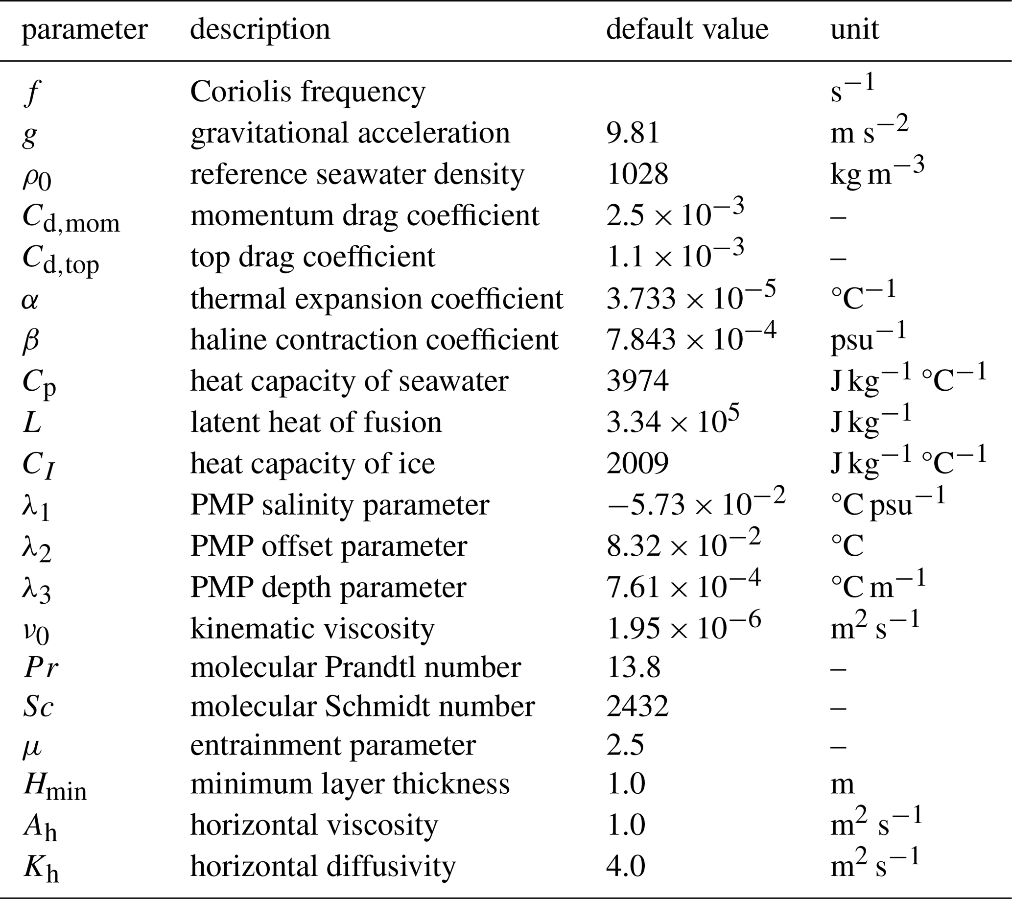
Several variables in these equations reflect input fields. The main geometric input field is the ice shelf draft H_ib, expressed as the height of the ice shelf base relative to sea-level. The position of the grounding line and calving front are derived from additional input fields, namely the ice thickness and the bed topography, from which a thickness of floatation is computed. Cells where the ice at the cell center (vertex) is floating, are included in the domain. This domain definition is equivalent to the floatation criterion melt parameterisation (FCMP,  Leguy et al., 2021) which was found to be most robust to changes in resolution in IMAU-ICE (Berends et al., 2023). As oceanic forcing, either 1D (vertical) or 3D fields of temperature and salinity are required. From these, the so-called ambient temperature and salinity T_a and S_a are determined at the depth of the mixed layer base through vertical interpolation.

The quasi-horizontal pressure gradient forces (first two right-hand side terms in the momentum equations) which drive the mixed layer velocities are buoyancy forces. $g_{\mathrm{a}}^{\prime }=g\frac{\mathrm{\Delta }{\mathit{\rho }}_{\mathrm{a}}}{{\mathit{\rho }}_{\mathrm{0}}}$ is the reduced gravity, where Δρ_a is the density difference between the mixed layer and the ambient water below the layer. This density difference is derived from the equation of state, for which we currently have only implemented a linear version:

$$\begin{array}{}\text{(6)}& \mathrm{\Delta }{\mathit{\rho }}_{\mathrm{a}}={\mathit{\rho }}_{\mathrm{0}}(-\mathit{\alpha }(T_{\mathrm{a}}-T)+\mathit{\beta }(S_{\mathrm{a}}-S\left)\right)\end{array}$$

As described above, T_a and S_a are derived from input forcing fields. More advanced expressions of the equation of state, such as that by Roquet et al. (2015) will be part of future model development.

2.3 Boundary conditions

At the top boundary, the ice shelf base, rates of melting or refreezing are derived from the commonly adopted three equations parameterisation (Holland and Jenkins, 1999; Jenkins et al., 2010):

$$\begin{array}{}\text{(7)}& {\displaystyle }{C}_{\mathrm{p}}{\mathit{\gamma }}_{\mathrm{T}}(T-T_{\mathrm{b}})=\dot{m}L+\dot{m}{C}_I(T_{\mathrm{b}}-T_{\mathrm{i}})\text{(8)}& {\displaystyle }{\mathit{\gamma }}_{\mathrm{S}}(S-S_{\mathrm{b}})=\dot{m}{S}_{\mathrm{b}}\text{(9)}& {\displaystyle }{T}_{\mathrm{b}}={\mathit{\lambda }}_{\mathrm{1}}{S}_{\mathrm{b}}+{\mathit{\lambda }}_{\mathrm{2}}+{\mathit{\lambda }}_{\mathrm{3}}{H}_{\mathrm{ib}}\end{array}$$

These three equations relate three unknowns: the melt or refreezing rate $\dot{m}$ and the temperature and salinity at the ice shelf base T_b and S_b. T_i is the temperature of the ice shelf interior. Note that recent insights into heat diffusion into the ice (Wiskandt and Jourdain, 2025) have not been implemented yet.

The turbulent exchange velocities of heat γ_T and salt γ_S (in m s⁻¹) can be a uniform tuning parameter, following the ISOMIP+ protocol (Asay-Davis et al., 2016), or they can be parameterised based on Jenkins (1991):

$$\begin{array}{}\text{(10)}& {\displaystyle }{\mathit{\gamma }}_{\mathrm{T}}={\displaystyle \frac{U_{*}}{\mathrm{2.12}\log (U_{*}H/{\mathit{\nu }}_{\mathrm{0}})+\mathrm{12.5}P{r}^{\mathrm{2}/\mathrm{3}}-\mathrm{8.68}}}\text{(11)}& {\displaystyle }{\mathit{\gamma }}_{\mathrm{S}}={\displaystyle \frac{U_{*}}{\mathrm{2.12}\log (U_{*}H/{\mathit{\nu }}_{\mathrm{0}})+\mathrm{12.5}S{c}^{\mathrm{2}/\mathrm{3}}-\mathrm{8.68}}}\end{array}$$

Note that other expressions for the turbulent exchange velocities (e.g.,  Jenkins et al., 2010) appear in the literature and these may be implemented during future development.

Finally, the friction velocity U_* in m s⁻¹ is defined as:

$$\begin{array}{}\text{(12)}& U_{*}=\sqrt{C_{\mathrm{d},\mathrm{top}}(U^{\mathrm{2}}+V^{\mathrm{2}}+U_{\mathrm{tide}}^{\mathrm{2}})}\end{array}$$

Here, C_d,top is the drag coefficient applied in the computation for basal melting, which functions as the primary tuning parameter of the model for total melt rates. U_tide is a time-mean tidal velocity in m s⁻¹ which can be provided as additional forcing.

At the mixed layer base, entrainment or detrainment is parameterised based on an expression for dense overflows (Gaspar, 1988), following the approach of Gladish et al. (2012):

$$\begin{array}{}\text{(13)}& {\displaystyle \frac{H}{\mathrm{2}}}{g}_{\mathrm{b}}^{\prime }\dot{m}+{\displaystyle \frac{H}{\mathrm{2}}}{g}_{\mathrm{a}}^{\prime }\dot{e}=\mathit{\mu }{U}_{*}^{\mathrm{3}}.\end{array}$$

To prevent the mixed layer thickness to become infinitely thin and cause numerical instabilities, we impose an artificial additional entrainment to ensure H≥H_min, where H_min is an input parameter, typically taken as 1 m.

Along the grounding line, in contrast to LADDIE 1.0, version 2.0 only has a no slip boundary condition. This assumption limits sub-shelf melting directly at the grounding line, in line with in-situ observations (Davis et al., 2023). Future observations in other regions can inform how valid the assumption of no slip is, or whether (partially) free slip boundary conditions should be implemented in v2.0 as well.

The final boundary condition applies at the calving front. Across this front, zero lateral gradients are applied to all main variables (H, U, V, T, and S).

2.4 Spatial discretisation

Spatially, the model is discretised on an unstructured mesh. This mesh is created by the Utrecht Polar SYstem (UPSY) toolbox, which is part of the same open-source repository in which LADDIE 2.0 is maintained and distributed. From the input geometry, the horizontal domain is divided into triangles through iterative refinement until certain requirements are met. Possible requirements are a maximum triangle size (leg length) on the ice shelf, and a maximum triangle size within a given band along the grounding line. Additionally, regions of interest can be prescribed to enhance the resolution of certain ice shelves or within specific regions of an ice shelf. Details on the mesh generation are described by Berends et al. (2025).

As visualised in Fig. 1, the ocean velocities are solved on these triangles. Most other variables, including the vertical exchanges $\dot{m}$ and $\dot{e}$ are resolved on cells surrounding the vertices of these triangles, which are Voronoi cells. Typically, the amount of triangles within a given model domain is approximately double the amount of Voronoi cells. A consequence of this mesh design is that the effective resolution of the velocity field is approximately a factor $\sqrt{\mathrm{2}}$ finer than that of other variables.

This spatial discretisation is equivalent to the Arakawa-B discretisation on square grids, and is the same as the discretisation in the 3D ocean model FESOM (Danilov et al., 2017). This is qualitatively different from LADDIE 1.0, which used an Arakawa-C discretisation. Following finite volume principles, horizontal advection is solved at the cell edges. Currently, only simple upstream-biased advection schemes are implemented for the advection of heat, salt, and momentum. Future model development may focus on more advanced schemes, though the presently available schemes have proved to be numerically stable in a wide variety of applications. We anticipate that more advanced advection schemes will allow for numerical stability with longer time steps, thereby providing an opportunity to further improve the computational efficiency in the future.

2.5 Temporal discretisation

Also the temporal discretisation in LADDIE 2.0 is different from that in LADDIE 1.0. In version 1.0, a modified LeapFrog scheme was implemented with a Robert–Asselin filter, similar to that in the 3D ocean model NEMO 4 (Madec et al., 2019). In version 2.0, we have replaced this with a third-order Forward–Backward Runge–Kutta scheme (FB-RK3,  Lilly et al., 2023) which is a generalised version of the regular third-order Runge–Kutta (RK3) scheme used in NEMO 5 (Madec et al., 2019).

We summarise the FB-RK3 scheme here in terms of a simplified set of equations for H and U, following Lilly et al. (2023) and refer to that study for an extensive discussion on this time stepping scheme.

Consider the simplified time derivatives

$$\begin{array}{}\text{(14)}& {\displaystyle \frac{\mathrm{d}H}{\mathrm{d}t}}=\mathrm{\Psi }(H,U)\text{(15)}& {\displaystyle \frac{\mathrm{d}U}{\mathrm{d}t}}=\mathrm{\Phi }(H,U)\end{array}$$

Then the time stepping is as follows:

$$\begin{array}{}\text{(16)}& {\displaystyle }{H}^{n+\mathrm{1}/\mathrm{3}}=H^n+{\displaystyle \frac{\mathrm{\Delta }t}{\mathrm{3}}}\mathrm{\Psi }(H^n,U^n)\text{(17)}& {\displaystyle }{U}^{n+\mathrm{1}/\mathrm{3}}=U^n+{\displaystyle \frac{\mathrm{\Delta }t}{\mathrm{3}}}\mathrm{\Phi }(H^{*},U^n)\text{(18)}& {\displaystyle }{H}^{*}={\mathit{\beta }}_{\mathrm{1}}{H}^{n+\mathrm{1}/\mathrm{3}}+(\mathrm{1}-{\mathit{\beta }}_{\mathrm{1}})H^n\text{(19)}& {\displaystyle }{H}^{n+\mathrm{1}/\mathrm{2}}=H^n+{\displaystyle \frac{\mathrm{\Delta }t}{\mathrm{2}}}\mathrm{\Psi }(H^{n+\mathrm{1}/\mathrm{3}},U^{n+\mathrm{1}/\mathrm{3}})\text{(20)}& {\displaystyle }{U}^{n+\mathrm{1}/\mathrm{2}}=U^n+{\displaystyle \frac{\mathrm{\Delta }t}{\mathrm{2}}}\mathrm{\Phi }(H^{**},U^{n+\mathrm{1}/\mathrm{3}})\text{(21)}& {\displaystyle }{H}^{**}={\mathit{\beta }}_{\mathrm{2}}{H}^{n+\mathrm{1}/\mathrm{2}}+(\mathrm{1}-{\mathit{\beta }}_{\mathrm{2}})H^n\text{(22)}& {\displaystyle }{H}^{n+\mathrm{1}}=H^n+\mathrm{\Delta }t\mathrm{\Psi }(H^{n+\mathrm{1}/\mathrm{2}},U^{n+\mathrm{1}/\mathrm{2}})\text{(23)}& {\displaystyle }{U}^{n+\mathrm{1}}=U^n+\mathrm{\Delta }t\mathrm{\Phi }(H^{***},U^{n+\mathrm{1}/\mathrm{2}})\text{(24)}& {\displaystyle }{H}^{***}={\mathit{\beta }}_{\mathrm{3}}{H}^{n+\mathrm{1}}+(\mathrm{1}-\mathrm{2}{\mathit{\beta }}_{\mathrm{3}})H^{n+\mathrm{1}/\mathrm{2}}+{\mathit{\beta }}_{\mathrm{3}}{H}^n\end{array}$$

Here, the weights β_k are called the forward–backward weights. In each of the three substeps above, first the thickness equations are solved. Next, the time-interpolated thickness H^* is determined. Finally, the momentum, heat, and salt equations are solved. To optimise numerical stability, the diffusive terms in the momentum, heat and salt equations are only determined at full timesteps n.

Based on extensive testing, Lilly et al. (2023) concluded that with values of approximately β₁=0.5, β₂=0.5, and β₃=0.33, numerical stability can be maintained with time steps approximately twice as large as with more commonly used RK3 schemes. The regular RK3 scheme can be approximated with β₁=0, ${\mathit{\beta }}_{\mathrm{2}}=\mathrm{2}/\mathrm{3}$, and β₃=0. Note that we have not performed any extensive testing on the maximum possible time step thus far, thereby leaving room for further improvement of the computational efficiency of LADDIE 2.0.

2.6 Integration with UFEMISM

We have chosen to fully integrate LADDIE 2.0 with the UFEMISM 2.0 ice sheet model (Berends et al., 2025) within the UPSY repository. Besides benefits related to the mesh generation capabilities, this allows for convenient coupled simulations, as illustrated in Sect. 4. One problem with coupled ice–ocean modelling is the large difference in time steps. For ice sheet models, these are typically on the order of a month to a year, whereas for high resolution ocean models, the time step is closer to a minute. Performing a regular coupled simulation therefore requires a very large amount of iterations of the ocean model for each ice sheet model iteration. We therefore integrate LADDIE for a shorter period than the actual coupling interval. During each coupling interval, the integration should be sufficiently long to achieve a new quasi-steady state. This method exploits the relatively rapid equilibration of LADDIE and substantially reduces the overall computation cost.

At each coupling time step, the ice geometry and temperature are provided by UFEMISM as forcing for LADDIE (Fig. 2). A simple wetting/drying scheme extrapolates LADDIE variables into any newly floating cells. In this scheme, when a cell changes from grounded to floating ice (wetting), H, T, and S are extrapolated from neighbouring floating cells; U and V are set to zero. In case of drying (floating ice turning into grounded ice), the cell is simply omitted from the domain without modifying surrounding floating cells. As this simple scheme may create relatively strong gradients in, e.g., velocities, LADDIE is integrated for a day with a reduced time step to avoid numerical instabilities. LADDIE is then integrated for a prescribed time period to sufficiently adjust the mixed layer toward the new ice geometry and, where applicable, new ambient ocean forcing. The resultant sub-shelf melt field is provided as forcing for UFEMISM. Time steps and required integration periods will depend on the model domain, characteristics, and resolution, and for each application, appropriate values should be found.

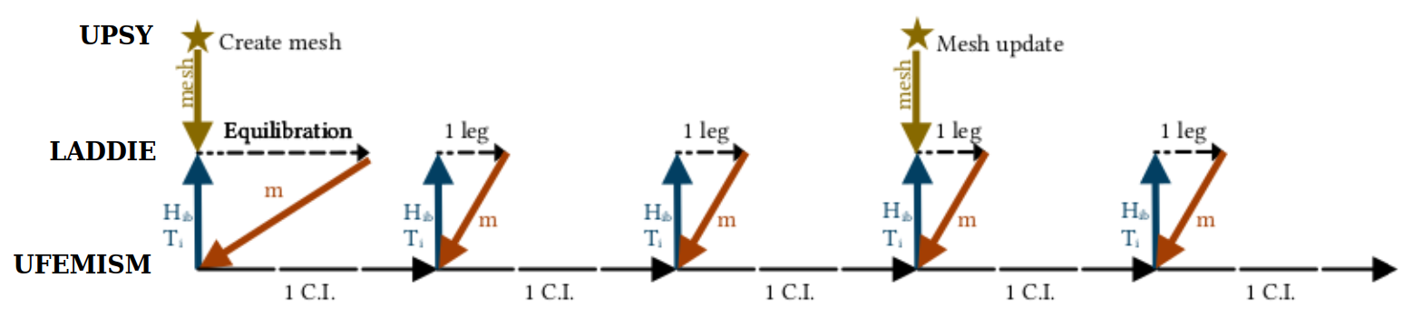
Figure 2 Illustration of the coupling strategy of UFEMISM and LADDIE. Dashed arrows indicate simulations of LADDIE and UFEMISM, the length of the dashes illustrates the time step, which ramps up during the first day of each LADDIE simulation. Coloured arrows indicate exchanged variables. C.I. stands for coupling interval.

Whenever a mesh update is triggered by UFEMISM, for example when the grounding line has retreated significantly, the primary variables in LADDIE (H, U, V, T, and S) are remapped using a second-order conservative scheme. After remapping the ice geometry as well, a short integration is performed to equilibrate the LADDIE variables to the new mesh. Except for the longer computational time (Sect. 4), running coupled UFEMISM/LADDIE simulations is as straightforward as running UFEMISM with a quadratic melt parameterisation.

3 Model evaluation

First, we perform a brief comparison to LADDIE 1.0 (Sect. 3.1), in order to ensure that the model has an improved computational performance without trade-off in terms of physical performance. We then evaluate LADDIE 2.0 against multi-model ensembles of 3D ocean models (Sect. 3.2) in both an idealised and a realistic pan-Antarctic setup. Finally, we evaluate LADDIE 2.0 against satellite-derived estimates of sub-shelf melting (Sect. 3.3) at pan-Antarctic scales, and at high resolution for which we take the Pine Island ice shelf as an example.

3.1 LADDIE v1.0

To compare the two versions of LADDIE, we perform a simulation of the Amundsen Sea region at 1 km for v1.0 and a maximum triangle size of 1.2 km (amounting to an equivalent resolution of approx 1.0 km) for v2.0. The geometry is taken from BedMachine v3 (Morlighem et al., 2020); in v1.0, the ice shelf domain is derived from the provided mask, whereas in v2.0, this domain is computed internally by UPSY based on the provided geometry. As ocean forcing, we use a tangent hyperbolic temperature profile describing a smooth thermocline centered at −450 m depth, separating an upper layer at surface freezing point from a lower layer at +1.0 °C. The model parameters are as in Lambert et al. (2023) and as specified in Table 1. The heat and salt transfer coefficients are defined as in Eq. (10). For both models, a uniform Coriolis parameter of −1.34 $\times {\mathrm{10}}^{-\mathrm{4}}$ s⁻¹ is applied. Both model versions are run for 20 d to achieve equilibrium.

The two versions of LADDIE show similar ocean currents (Fig. 3a–c) and very similar melt patterns (Fig. 3d–f). A close examination (Fig. 3c) shows that ocean speeds in v2.0 are 10 %–20 % stronger on average. This is likely related to the higher effective resolution of the velocity field due to the unstructured mesh (Sect. 2.4). These higher currents also lead to melt rates in v2.0 which are 5 %–15 % stronger (Fig. 3d–e). Additionally, the stronger currents enhance the Coriolis deflection of melt plumes, causing stronger melting along the Western margins of ice shelves (Fig. 3f). Individual melt plumes are also more sharply defined in v2.0, due to the higher effective resolution of the velocity field.

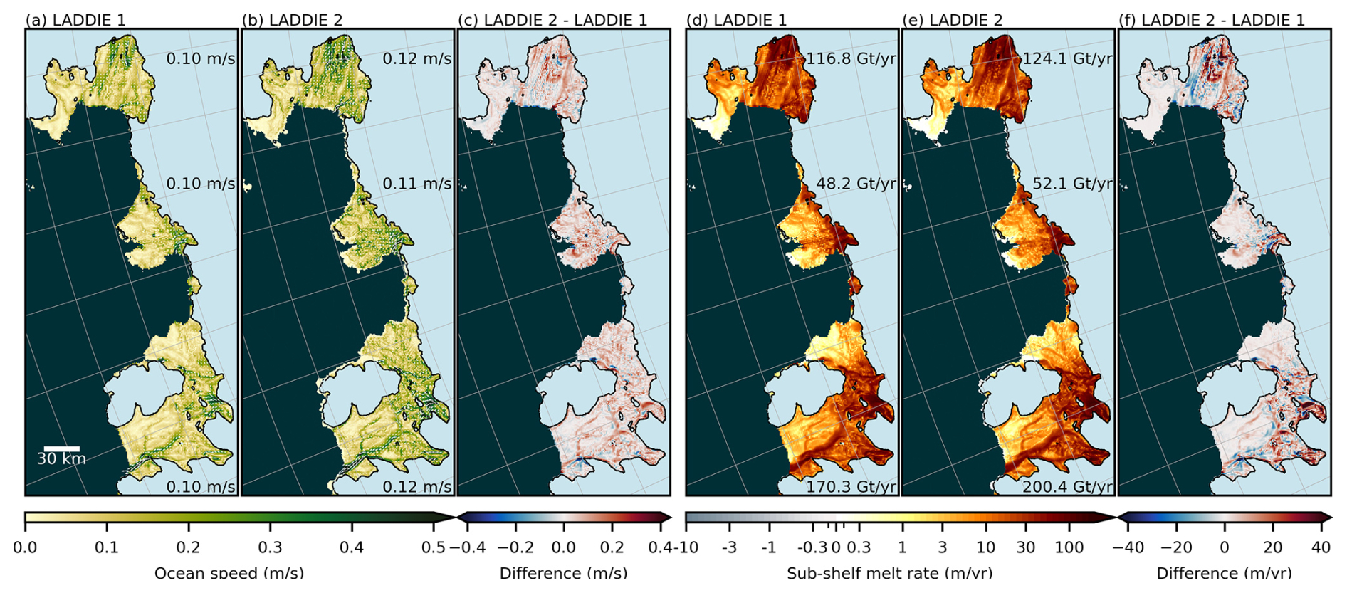
Figure 3 Amundsen Sea comparison between LADDIE 1.0 and LADDIE 2.0. Ocean speeds from (a) LADDIE 1.0, (b) LADDIE 2.0, and (c) the difference between the two model versions. White velocity vectors in (a) and (b) indicate the direction of the upper ocean flow. Average values for the Pine Island (top), Thwaites (middle), and Crosson–Dotson (bottom) ice shelves are noted. Sub-shelf melt rates for (d) LADDIE 1.0, (e) LADDIE 2.0, and (f) the difference. The numbers in (d) and (e) are integrated melt rates for the same three ice shelves. For visual reference, the grounding line (black line) as determined by LADDIE 2.0 is shown in each panel. Light blue colors denote grounded ice, dark green colors denote open ocean.

Besides differences in effective resolution, the different spatial discretisation of v2.0 compared to v1.0 induces unavoidable differences in the treatment of input geometry (which is remapped from a squre grid to an unstructured mesh in v2.0) and boundary conditions along the grounding line and calving front. However, we deem all of these differences to be minor in terms of the simulated melt rates and melt patterns, concluding that no notable changes can be detected in the model quality itself. That said, in order to accurately reproduce melt rates from, e.g., satellite estimates, the two models should be tuned separately for an optimal result.

To compare the computational time of the two model version, we have run the Amundsen Sea simulation with v2.0 at a different number of cores (Fig. 4). At a single core, v2.0 is slightly faster than v1.0 which can only be run on a single core. This is likely related to the unstructured mesh. Whereas this discretisation requires approximately twice as many computations of velocity, it requires significantly fewer computations over grounded ice and open ocean. The net effect appears to be dominated by the latter benefit for this specific example. Additionally, the transition from an interpreted language (Python) to a compiled language (Fortran) may have contributed to the performance improvement.

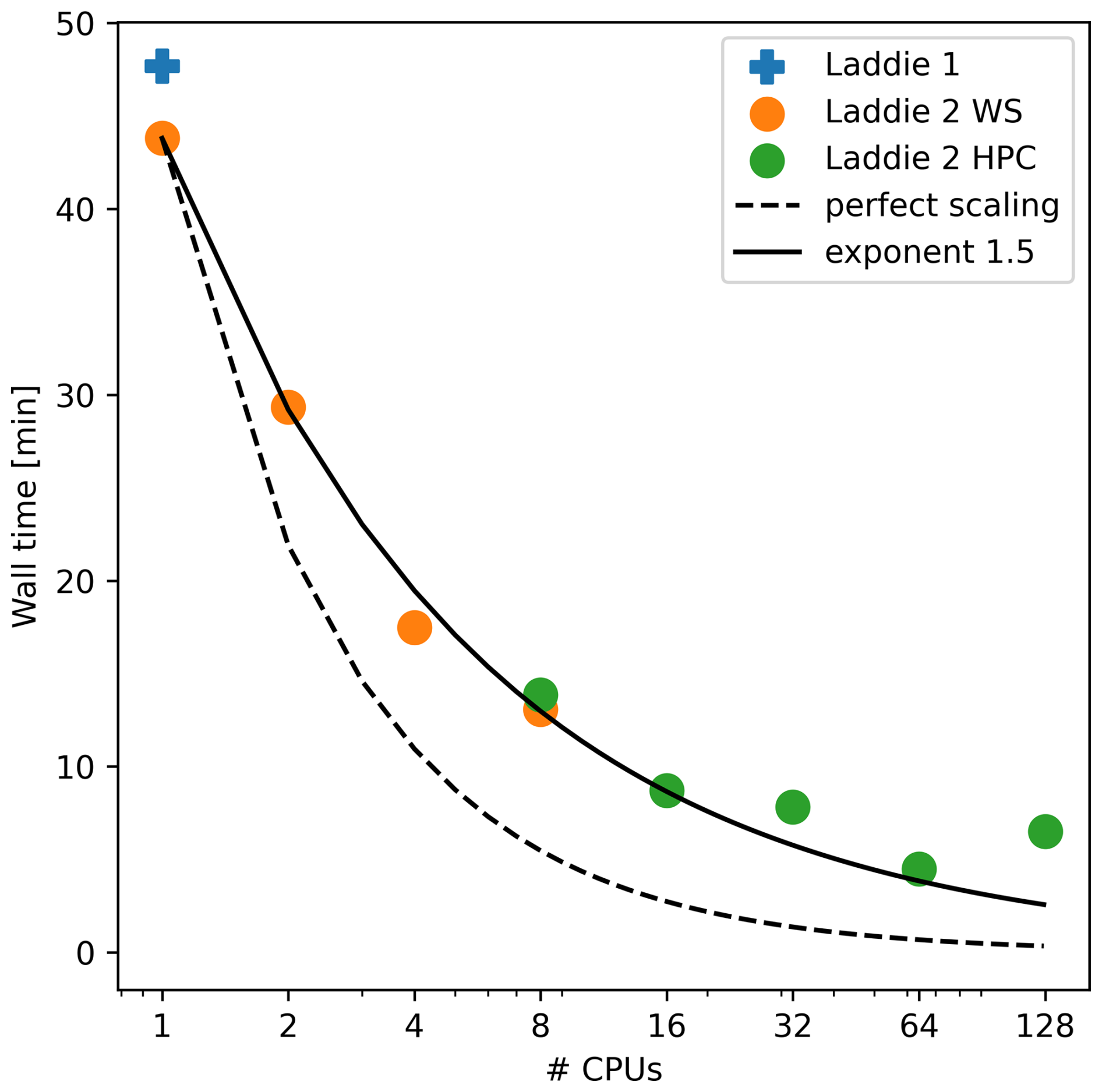
Figure 4 Computation times of the Amundsen Sea simulation. LADDIE 1.0 can only be run on 1 core, and was run on a workstation (Dell Precisison 5690 with Intel^® Core^™ Ultra 7 165H processors). LADDIE 2.0 was run on the same workstation on 1, 2, 4, and 8 cores. Additionally, it was run on an HPC (ECMWF H2020 Atos with AMD Epyc Rome processors) on 8, 16, 32, 64, and 128 cores.

The main computational improvement though, stems from the parallellisation. For the Amundsen Sea example, containing approximately 30 000 vertices and 60 000 triangles, a doubling of the amount of cores produces an approximate reduction in computing time of 33 %, until 64 cores, beyond which the computing time increases. However, we see a minimal speed up from 16 to 32 cores, and for this specific example, 16 cores is arguably the optimal trade-off between computing time and resources. The limited scaling of the UPSY parallellisation for more cores is described in detail by Berends et al. (2025). Further improving this scaling is the focus of continued development. In various test runs at various resolutions, the most rapid simulations were achieved systematically at 32 or 64 cores, though we cannot exclude the possibility of configurations where 16 or 128 cores would be the optimal configuration. This should therefore be optimised for each use case. Overall, we conclude that at present, the simulation time can be reduced by one order of magnitude, compared to LADDIE 1.0.

3.2 3D ocean models

3.2.1 Idealised domain

To compare cavity-resolving 3D ocean models and their simulated sub-shelf melt rates, the second Ice Shelf-Ocean Model Intercomparison Project (ISOMIP+, Asay-Davis et al., 2016) was designed. This experimental protocol prescribes an idealised ice shelf geometry of 80 km width and approximately 180 km length. Alongside, linear profiles in temperature and salinity are prescribed as offshore forcing. The results of 12 ocean models are described by Yung et al. (2025).

Here, we reproduce the Ocean1 COM experiment, which is a steady-state experiment with warm ocean forcing, mimicking Amundsen Sea conditions. Following the original protocol, we take C_d,top = 2.5 $\times {\mathrm{10}}^{-\mathrm{3}}$ and use uniform heat and salt coefficients for tuning the average melt rates to 30 ± 2 m yr⁻¹ in the region where the draft extends below H_ib= −300 m. This tuning exercise leads to a heat transfer coefficient Γ_T = 2.78 $\times {\mathrm{10}}^{-\mathrm{2}}$, producing an average melt rate at depth of 30.02 m yr⁻¹. Note that this value of Γ_T is close to the theoretically derived value of 2.2 $\times {\mathrm{10}}^{-\mathrm{2}}$ in Asay-Davis et al. (2016). The turbulent heat exchange velocity is then computed as ${\mathit{\gamma }}_{\mathrm{T}}={\mathrm{\Gamma }}_{\mathrm{T}}{U}_{*}$. Following the protocol, the salt transfer coefficient is defined as ${\mathrm{\Gamma }}_{\mathrm{S}}={\mathrm{\Gamma }}_{\mathrm{T}}/\mathrm{35}$.

LADDIE 2.0 is configured at a maximum triangle size of 2.0 km, and its output fields are remapped to the common square grid of 2.0 km. The offshore forcing profiles are extrapolated into the cavity, following the general practice of ISMIP6 (Jourdain et al., 2020). The model is run for 20 model days, which is sufficient to achieve equilibrium. This simulation takes 32 s on a workstation at 8 cores. A comparison to the multi-model mean (Fig. 5) shows that LADDIE represents the typical melt patterns simulated by the various models well.

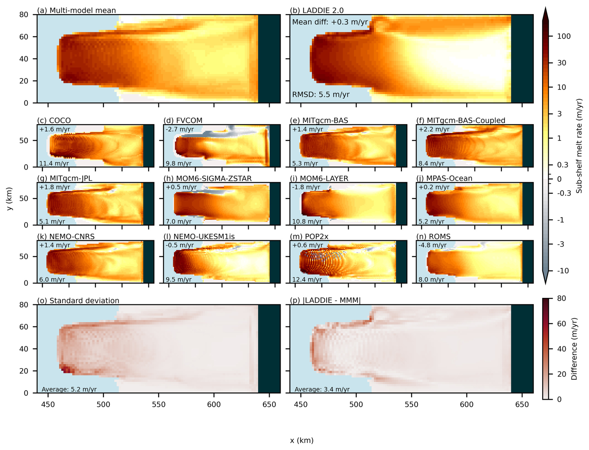
Figure 5 A comparison with 3D models based on the ISOMIP+ Ocean1 experiment. (a) The multi-model mean sub-shelf melt rates of 12 ocean models. (b) The results of LADDIE 2.0. (c–n) The results of the individual models. (o) The standard deviation of the 12 models. (p) The absolute difference between LADDIE 2.0 and the multi-model mean. In panels (b)–(n), two bulk quantities are included: the top number is the mean difference with respect to the multi-model mean; the bottom number is the root mean squared difference.

To first order, all models (Fig. 5c–n) simulate the depth-dependency of sub-shelf melting, reflected by a gradient from high melting close to the grounding line (left-hand side) to low melting toward the calving front (right-hand side). In two regions, a substantial disagreement is found between the 3D ocean models: in the lower left corner, and in the boundary current at y≈ 60 km. In these two regions, the multi-model mean melt rates are highest (Fig. 5a), as well as the standard deviation between the models (Fig. 5o). Even qualitative differences appear, as a subset of models simulates refreezing rather than melting along the boundary current (Fig. 5d, h, n). Mean differences from the multi-model mean range from −4.8 to +2.2 m yr⁻¹ and root mean squared differences of the spatial melt patterns range from 5.1 to 12.4 m yr⁻¹.

The general melt pattern of LADDIE (Fig. 5b) closely resembles that of the multi-model mean. This resemblance is confirmed by the relatively low root mean squared difference of 5.5 m yr⁻¹. Additionally, the mean difference between LADDIE and the multi-model mean is +0.3 m yr⁻¹. Hence, in terms of both metrics, LADDIE ranks among the models closest to the multi-model mean.

The spatial difference between LADDIE and the multi-model mean (Fig. 5p) is generally smaller than the standard deviation between the 3D models (Fig. 5o). One region where LADDIE deviates from the ensemble is the shape of the boundary current at the top of the domain, where the boundary current tracks the grounding line and model domain. This can be partly explained by different boundary current dynamics and partly by the fact that in some models, the geometry along this boundary is smoothed. In addition, approximately half of the 3D ocean models produce zero melting close to the deepest grounding line (Fig. 5c, d, h, i, n), leading to relatively low melt rates in the multi-model mean close to the grounding line at y= 40 km. The behaviour of LADDIE is most similar to the half of the models that simulate strong melting at the grounding line. To what extent sub-shelf melting vanishes close to the grounding line is still an open question, so how realistic the behaviour of LADDIE is cannot be evaluated.

Overall, a subset of four models (MITgcm-BAS, MITgcm-JPL, MPAS-Ocean, and NEMO-CNRS) simulate highly similar melt patterns and average melt rates, which are close to the multi-model mean. We find that LADDIE can reproduce these melt patterns and melt rates, illustrating a capability to reproduce some of the essential physics establishing these melt patterns.

3.2.2 pan-Antarctic domain

A suite of modelling groups have simulated pan-Antarctic sub-shelf melt rates using 3D ocean models, from which Galton-Fenzi et al. (2025) constructed a multi-model ensemble called RISE (Realistic Ice-shelf/ocean State Estimate). This analysis includes a multi-model mean reference and an intercomparison of several bulk metrics including ocean speeds, hydrographic properties, and melt sensitivities. Here, we perform a comparison run at pan-Antarctic scale and diagnose equivalent bulk metrics from LADDIE 2.0.

The model is set up with the Bedmachine v3 geometry (Morlighem et al., 2020). A mesh is created with a maximum triangle size of 3 km, amounting to a resolution of approximately 2 km. This mesh consists of 452 846 vertices and 905 546 triangles. As ocean forcing, we use the extrapolated climatology of ISMIP6 (Jourdain et al., 2020; Seroussi et al., 2024). The model configuration is as in Table 1.

Besides sub-shelf melting, distributions in ocean currents, temperatures, and salinities were compared between the models. These bulk metrics from RISE and LADDIE are listed in Table 2.

Table 2 Comparison to RISE (Galton-Fenzi et al., 2025). The melt sensitivities are derived from the spatial pattern, defined as $\mathit{\zeta }=m\left(U^{*}\right(T-T_{\mathrm{f}}){)}^{-\mathrm{1}}$ and $\mathit{\psi }=m(T-T_{\mathrm{f}}{)}^{-\mathrm{1}}$. MMM: multi-model mean.

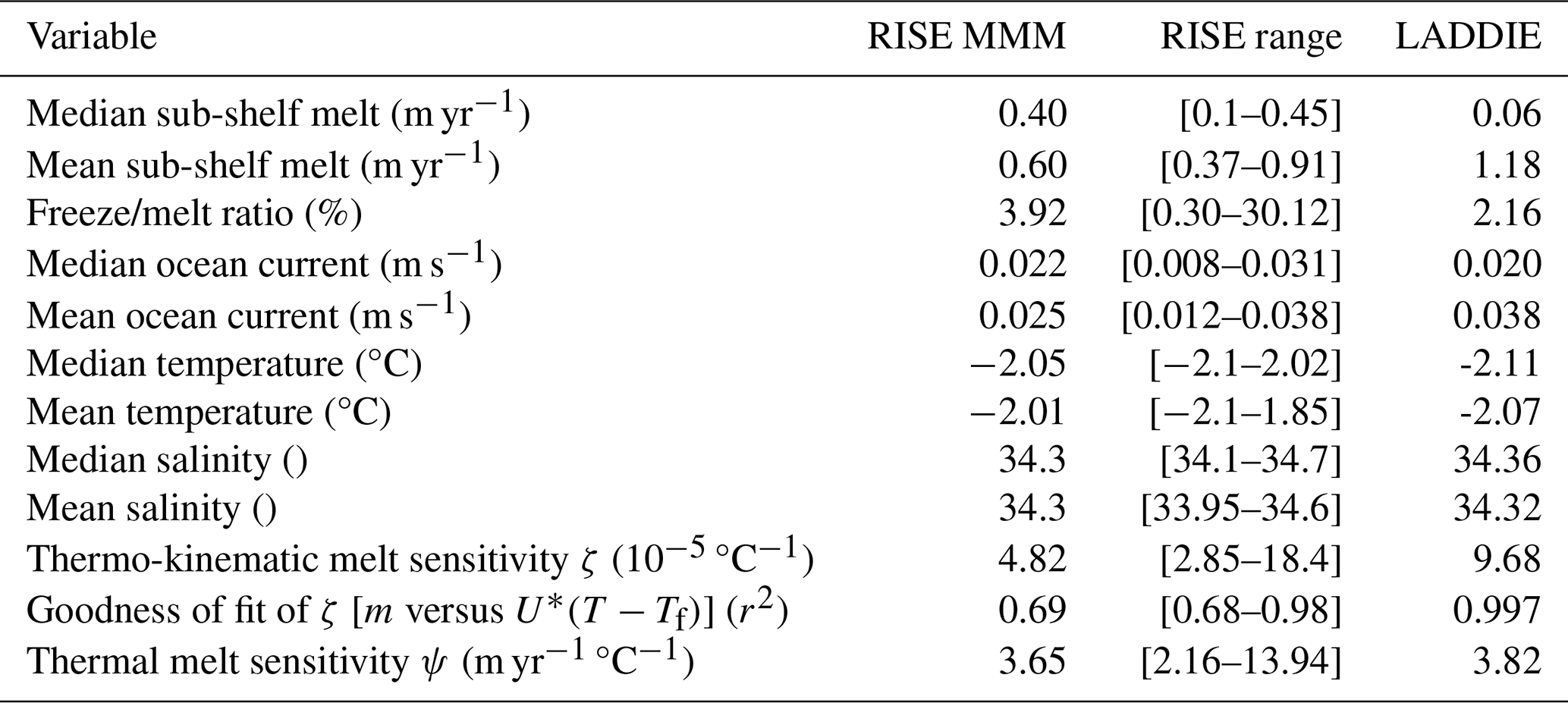
In LADDIE, the median ocean current is very similar to the RISE ensemble, though mean ocean currents are comparable to the two models with the highest current speeds (COCO and FESOM-HR). We attribute these relatively strong ocean currents partially to the higher effective resolution of the velocity field (approx. 1.5 km), compared to the resolution of the melt field. The temperatures in LADDIE are at the lower end of the ensemble, while the salinities are very close to the multi-model mean.

The mean melt rates of LADDIE are higher than the multi-model ensemble. A comparison to satellite estimates (Sect. 3.3) shows that these relatively high melt rates are likely caused by regional biases, either in LADDIE or in the applied ocean forcing. The major discrepancies are found along the Bellingshausen Sea (#6–9 in Fig. 6c), the Amundsen Sea (#12–14), and at the Borchgrevink ice shelf (#32). The overestimation of LADDIE melt rates along the Bellingshausen Sea and at the Borchgrevink ice shelf is also seen in comparison to satellite estimates (Fig. 7c). This is in part caused by a warm bias in the ISMIP6 forcing dataset, which contains a shallower thermocline in these regions than the more recent compilation of observations by Zhou et al. (2025). First tests with preliminary ISMIP7 forcing show a significant reduction in LADDIE melt rates at these ice shelves (not shown).

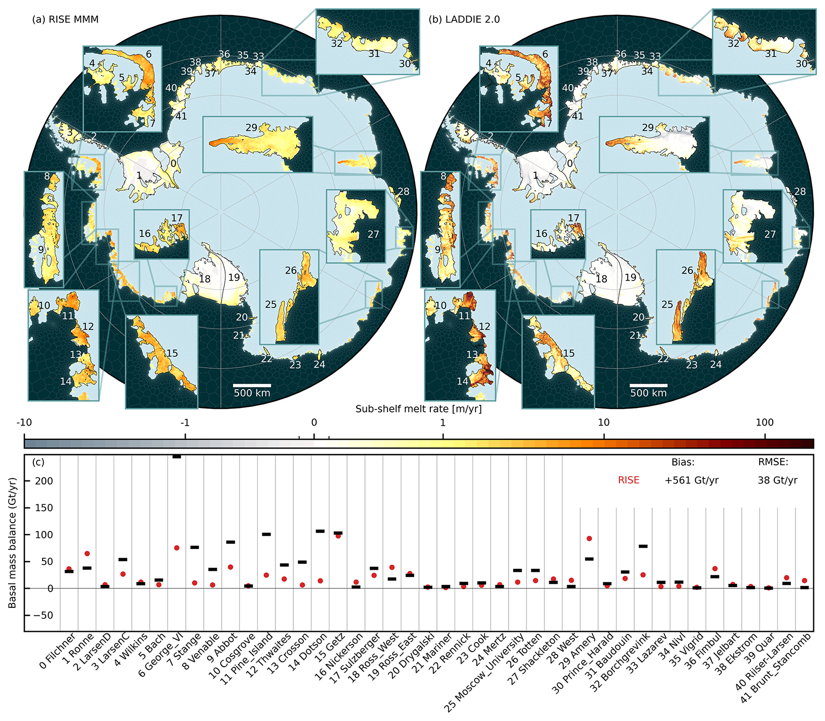
Figure 6 pan-Antarctic melt rates compared to 3D ocean models. (a) Multi-model mean from RISE (Galton-Fenzi et al., 2025). (b) Model results from LADDIE 2.0. Ice shelf boundaries (black) are derived from Measures (Mouginot et al., 2017). (c) A comparison of basal mass balance from LADDIE (black bars) to the RISE multi-model mean (red dots). The bulk metrics in the top right denote the bias in total basal mass balance of LADDIE with respect to RISE, and the root mean squared error in basal mass balance of individual ice shelves.

We also find a large difference in median melt rates between the RISE ensemble and LADDIE. This median value reflects the typical melt rates in the relatively flat and shallow regions of ice shelves. A notable example is the Amery ice shelf (#29), where 3D ocean models simulate melting on the order of 1 m yr⁻¹, whereas LADDIE simulates near-zero melt rates. A similar discrepancy is found in the idealised ISOMIP+ configuration (Fig. 5). We attribute this difference to underestimated temporal variability in LADDIE, which converges to a nearly static steady state, whereas ocean models retain a considerable temporal variability in ocean speeds. This variability can induce a net transport of heat towards otherwise cold shallow regions, along with non-zero friction velocities. A specific example of how variability causes enhanced melting is “mode 3” melting, induced by seasonal intrusions of warm water into the shallow regions of the cavity, which is not represented by LADDIE. Because these regions typically contribute little to buttressing, we consider this discrepancy of lesser importance.

The discrepancy in Amundsen Sea melt rates appears to reveal a low-melt bias in the 3D ocean models, as LADDIE shows a good comparison to satellite estimates (Fig. 7c). These low melt rates may result from the inclusion of relatively low resolution ocean models which struggle to simulate the high melt rates at the small Amundsen Sea ice shelves. Altogether, 8 out of 9 models in the RISE ensemble underestimate melt rates compared to satellite estimates. This is partly attributed by Galton-Fenzi et al. (2025) to post-processing and discrepancies between originally published melt rates and those reported in RISE.

The ratio between total refreezing and total melting varies greatly between the individual models (Table 2), though a clustering of 5 out of 9 models report values between 2 % and 5.5 %. LADDIE produces relatively low values compared to this ensemble (2.16 %), which is likely caused by an underestimation of refreezing at the Filchner–Ronne and Ross ice shelves (see Fig. 7a, b) due to an underestimation of the barotropic currents and tides in these cavities.

A primary result of Galton-Fenzi et al. (2025) is the quantification of two melt sensitivities: the thermo-kinetic and the thermal sensitivity. The former is defined as $\mathit{\zeta }=m/\left(\right(T-T_{\mathrm{f}}\left)U_{*}\right)$. The thermo-kinetic melt sensitivity of LADDIE is close to the ensemble median of 8.60  $\times {\mathrm{10}}^{-\mathrm{5}}$ °C⁻¹. Notably, the goodness of fit between melt rates and the thermo-kinetic driving is substantially higher than that of each individual model. This may be a reflection of the relatively simple physics embedded in LADDIE compared to 3D ocean models. We should note that remapping the fields to a squared 2 km grid, as is done in RISE, reduces this goodness of fit to 0.98, similar to 3 of the 9 models.

The thermal sensitivity, more commonly used in parameterisations, is determined by using the average value of U_*. Here, the LADDIE value is very close to the multi-model mean. The agreement between LADDIE and RISE does hide some discrepancy though, as LADDIE produces higher current speeds. The lower drag coefficient than used in most models, however, produces comparable average friction velocities.

In terms of most bulk metrics, the simulations of LADDIE produce values close to the multi-model mean of the RISE ensemble of 9 3D ocean models. The primary differences are the higher mean current speeds and the higher average melt rates. To evaluate these higher melt rates, we now perform an in-depth comparison to four remote sensing data sets.

3.3 Satellite estimates

3.3.1 pan-Antarctic domain

We have compared the same pan-Antarctic simulation as presented in Sect. 3.2.2 to four remote sensing products (Rignot et al., 2013; Adusumilli et al., 2020; Paolo et al., 2023; Davison et al., 2023) (Fig. 7). As only Adusumilli et al. (2020) and Paolo et al. (2023) provide publicly available gridded melt maps, and the latter is commonly interpreted as an update of the former, we compare spatial patterns of LADDIE to the remote sensing estimates of Paolo et al. (2023), rather than an average of multiple products (Fig. 7a). We note that the agreement between LADDIE with the other three satellite products is better than the agreement with Paolo et al. (2023) (Fig. 7c).

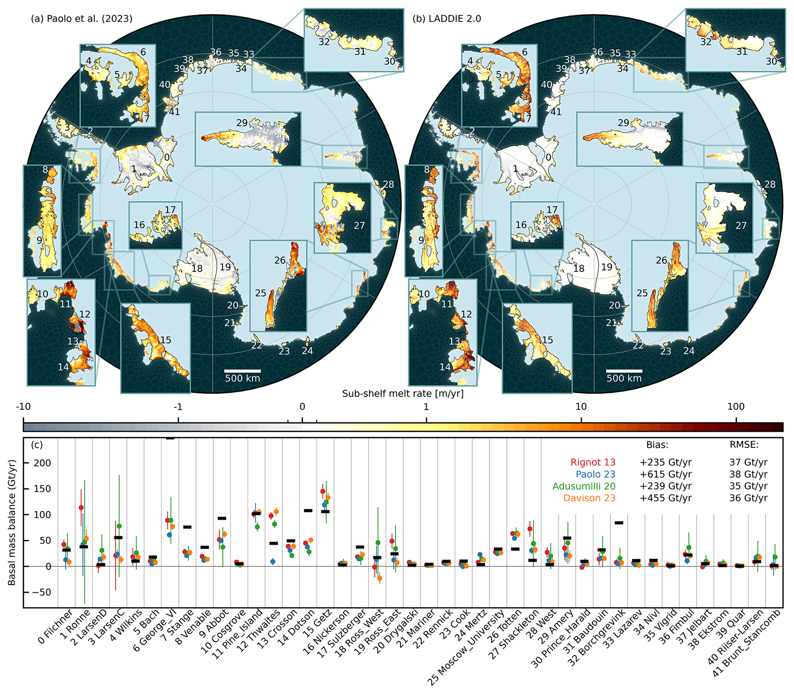
Figure 7 pan-Antarctic melt rates. (a) Remote sensing estimates by Paolo et al. (2023). (b) Model results from LADDIE 2.0, as in Fig. 6. Ice shelf boundaries (black) are derived from Measures (Mouginot et al., 2017). (c) A comparison of basal mass balance from LADDIE (black bars) to observations for individual ice shelves. Observations are from Rignot et al. (2013); Paolo et al. (2023); Adusumilli et al. (2020); Davison et al. (2023). The bulk metrics in the top right denote the bias in total basal mass balance of LADDIE with respect to individual remote sensing products, and the root mean squared error in basal mass balance of individual ice shelves.

The integrated basal mass balances (Fig. 7c) show a similar discrepancy as when compared to 3D models. The dominant discrepancy is along the Bellingshausen Sea (#6–9) and at the Borchgrevink ice shelf (#32). As described in Sect. 3.2, we attribute this discrepancy at least partly to biases in ocean forcing, and preliminary results indicate that this discrepancy can be significantly reduced using updated forcing. In addition, LADDIE produces higher basal mass balances for the Crosson and Dotson ice shelves. This is due to the fact that remote sensing products typically omit the deepest, fast melting part of these ice shelves, as is visible by the white space on ice shelves #13 and 14 in Fig. 7a. A final notable discrepancy is visible at Totten ice shelf. This may be caused by the absence of recent warm water observations by Hirano et al. (2023) in the ISMIP6 forcing product.

As seen in the comparison to 3D models, LADDIE underestimates the extent and magnitude of refreezing in cold cavities, such as Filchner–Ronne (#0–1), Ross (#18–19), and Amery (#29). This bias is confirmed in the comparison to the satellite-derived melt patterns (Fig. 7a). Additionally, mode 3 melting in the shallow parts of ice shelves close to the calving front (Jacobs et al., 1992) is not represented. This is best visible at, for example, the Ronne (#1) and Shackleton (#27) ice shelves. As both mode 3 melting and refreezing occur in regions away from the grounding line, we consider these discrepancies to be of limited influence on ice sheet model behaviour.

One feature that is underrepresented in large-scale remote sensing products is basal channels (Zinck et al., 2024). At many ice shelves around Antarctica, the basal topography is marked by channels in which basal melting is known to be enhanced (e.g.,  Alley et al., 2022). Such channelised melting is simulated by LADDIE (Fig. 7b), and reported previously in higher resolution studies (Lambert et al., 2023; Zinck et al., 2024, 2025). To evaluate channelised melting of LADDIE 2.0 properly, we therefore resort to regional remote sensing products for the Pine Island ice shelf.

3.3.2 Pine Island ice shelf

We choose the Pine Island ice shelf as a case study for high-resolution evaluation of melt patterns, as multiple studies have produced remote sensing-based melt estimates. To perform a high resolution simulation, we have taken the surface geometry from the REMA mosaic (Howat et al., 2019). This geometry is combined with bathymetry from Bedmap v3 (Pritchard et al., 2025), interpolated onto the 100 m REMA grid. Ice thickness is derived assuming a uniform ice density of 917 kg m⁻³ and a uniform seawater density of 1027 kg m⁻³, ignoring any firn air content for simplicity.

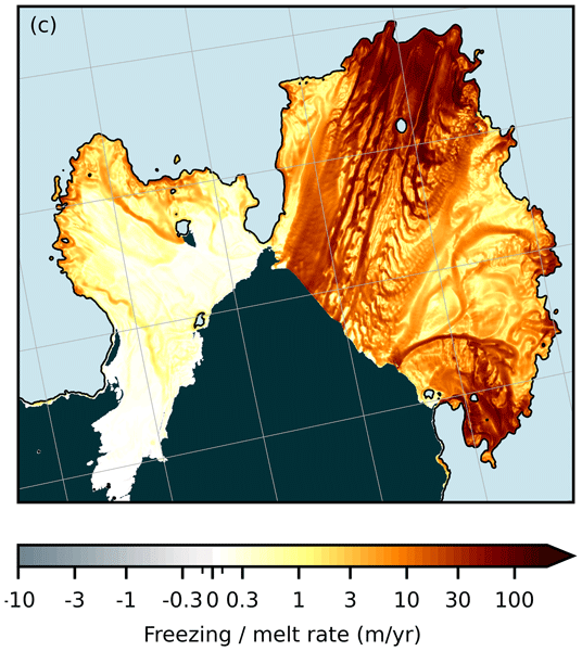
LADDIE is run with a maximum triangle size of 150 m on the ice shelf, which results in a mesh with a nominal resolution of 120 m for the thickness cells, and 80 m for the velocity triangles. In total, the mesh consists of 433 548 vertices and 866 972 triangles. The ocean forcing is idealised, and identical to that described in Sect. 3.1. The remaining model configuration is as described in Table 1.

For comparison, we include two separate high resolution satellite estimates from Shean et al. (2019); Zinck et al. (2024) (Fig. 8a, b). Both satellite estimates show a fine-grained pattern of channelised melting which is dominated by relatively few along-ice-flow channels in the deep and central region, which branch off in a higher number of narrower channels which deflect in both directions. This deflection is partly governed by Coriolis deflection (towards the left of the meltwater flow), and partly by topographic steering up-slope (both directions). LADDIE simulates a qualitatively comparable field of melt patterns, with few wide channels along-ice-flow, which branch into a large number of narrow channels in both directions. Also concentrated melting within the well-known Y-shaped channel, best visible in the pattern of Shean et al. (2019) is clearly resolved in LADDIE. Additional channels in the southern shear margin (upstream from the Y-shaped channel) are simulated due to topographic guidance. These shear margins are heavily damaged, breaking the assumption of continuity necessary to derive melt rates from satellite altimetry. The realism of these channels can therefore not be evaluated from satellite products.

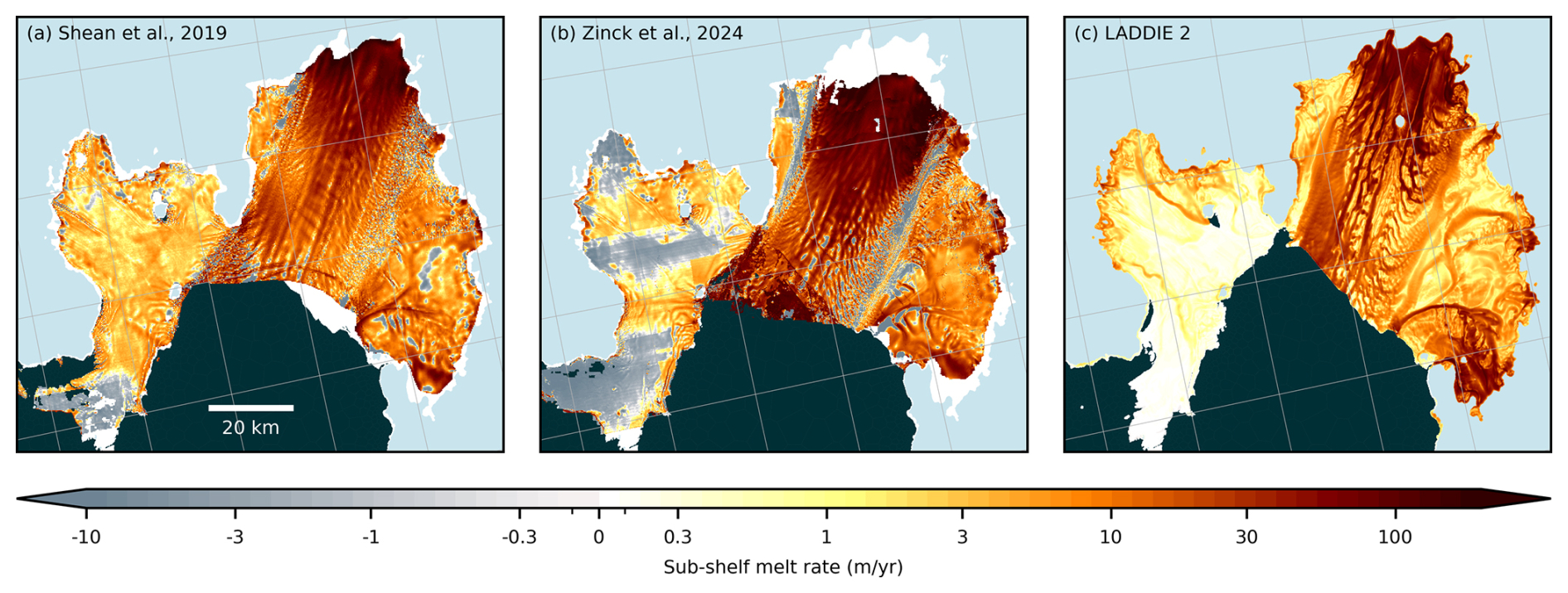
Figure 8 Pine Island sub-shelf melt rates. (a) Satellite estimates from Shean et al. (2019). (b) Satellite estimates from Zinck et al. (2024). (c) Model results from LADDIE 2.0.

The comparison reveals two problems in the evaluation to satellite estimates. First, an exact, quantitative comparison at grid cell level is complex, as geometries are derived over different periods. Correcting for geometric changes over these periods (e.g., Zinck et al., 2025) is beyond the scope of this model description paper. Second, the method of estimating sub-shelf melt rates from changes in satellite altimetry does not allow for estimating melt rates close to the grounding line. The estimation of melt rates relies on the assumption of hydrostatic balance, which breaks down within a band of multiple kilometres around the grounding line due to bridging stresses. Satellite estimates can therefore not be used to evaluate modelled basal melt rates in these regions, which are possibly the most important for ice sheet stability. For this, in-situ observations are needed which at present are scarce (Davis et al., 2023).

4 Coupled ice–ocean simulations

To illustrate the coupled UFEMISM–LADDIE behaviour, we perform the idealised MISOMIP+ simulations (Asay-Davis et al., 2016) with modified ocean forcing following Jesse et al. (2025). In these experiments, an ice sheet and ice shelf are initialised with the same bedrock topography as the ISOMIP+ configuration (Sect. 3.2.1) and a uniform surface mass balance of 0.3 m yr⁻¹.

UFEMISM is configured with the depth-integrated viscosity approximation (DIVA, Goldberg, 2011), and the Zoet-Iverson sliding law (Zoet and Iverson, 2020). A full configuration file containing all details is provided in (Lambert, 2026). An initial state is produced by integrating UFEMISM for 20 000 years with zero sub-shelf melting, and by modifying Glen's flow factor A iteratively to ensure a central grounding line position at x= 450 km, which converges to $A=\mathrm{1.96}\times {\mathrm{10}}^{-\mathrm{17}}$. After this spinup, sub-shelf melting is applied by imposing an idealised ocean forcing to either LADDIE or a quadratic melt parameterisation, as described below. Here, we apply the idealised high-melt forcing of Jesse et al. (2025), which represents a smooth two-layer temperature profile in which an upper layer at surface freezing point is separated from a lower layer at 1.2 °C by a smooth thermocline, centered at −450 m depth. The simulations with high-melt ocean forcing are run for 300 years following the spinup.

The resolution over the grounded ice is set by a maximum triangle size of 8 km; over the ice shelf, this is 1 km. As the grounding line retreats, the ice shelf expands into the region of coarser resolution. At each time step, UFEMISM determines a mesh fitness coefficient, quantifying the percentage of cells adhering to the prescribed resolution requirements. When this mesh fitness drops below a user-provided value (in our case 0.95), a mesh update is triggered (Fig. 2). Sub-shelf melt forcing is computed either by LADDIE 2.0, or by the quadratic melt parameterisation. In both cases, the melt rates are tuned following the MISOMIP+ protocol, to ensure an average melting of 30 m yr⁻¹ in the region where the ice draft is deeper than −300 m. For LADDIE, this resulted in ${\mathrm{\Gamma }}_{\mathrm{T}}=\mathrm{2.03}\times {\mathrm{10}}^{-\mathrm{2}}$, while keeping C_d,top fixed at $\mathrm{2.5}\times {\mathrm{10}}^{-\mathrm{3}}$. For the quadratic parameterisation, this leads to ${\mathit{\gamma }}_{\mathrm{T}}=\mathrm{3.9}\times {\mathrm{10}}^{-\mathrm{4}}$ m s⁻¹.

With both melt options, the ice shelf thins, leading to a steepening of the basal slope in the deepest ice shelf region (Fig. 9). The ice shelf thinning induces a reduction in buttressing, allowing for higher ice speeds, which in turn cause a retreat of the grounding line. Quantitatively, a considerable difference appears between the quadratic melt parameterisation and LADDIE. For the quadratic parameterisation, ice shelf thinning raises the ice draft out of the warm ocean layer, leading to suppressed melting except in the very deepest regions (Fig. 9n, o, p). With the quadratic parameterisation, ice shelf thinning thus induces a negative feedback. The resultant melt suppression eventually leads to a minimal speed up of the ice flow (Fig. 9v, w, x).

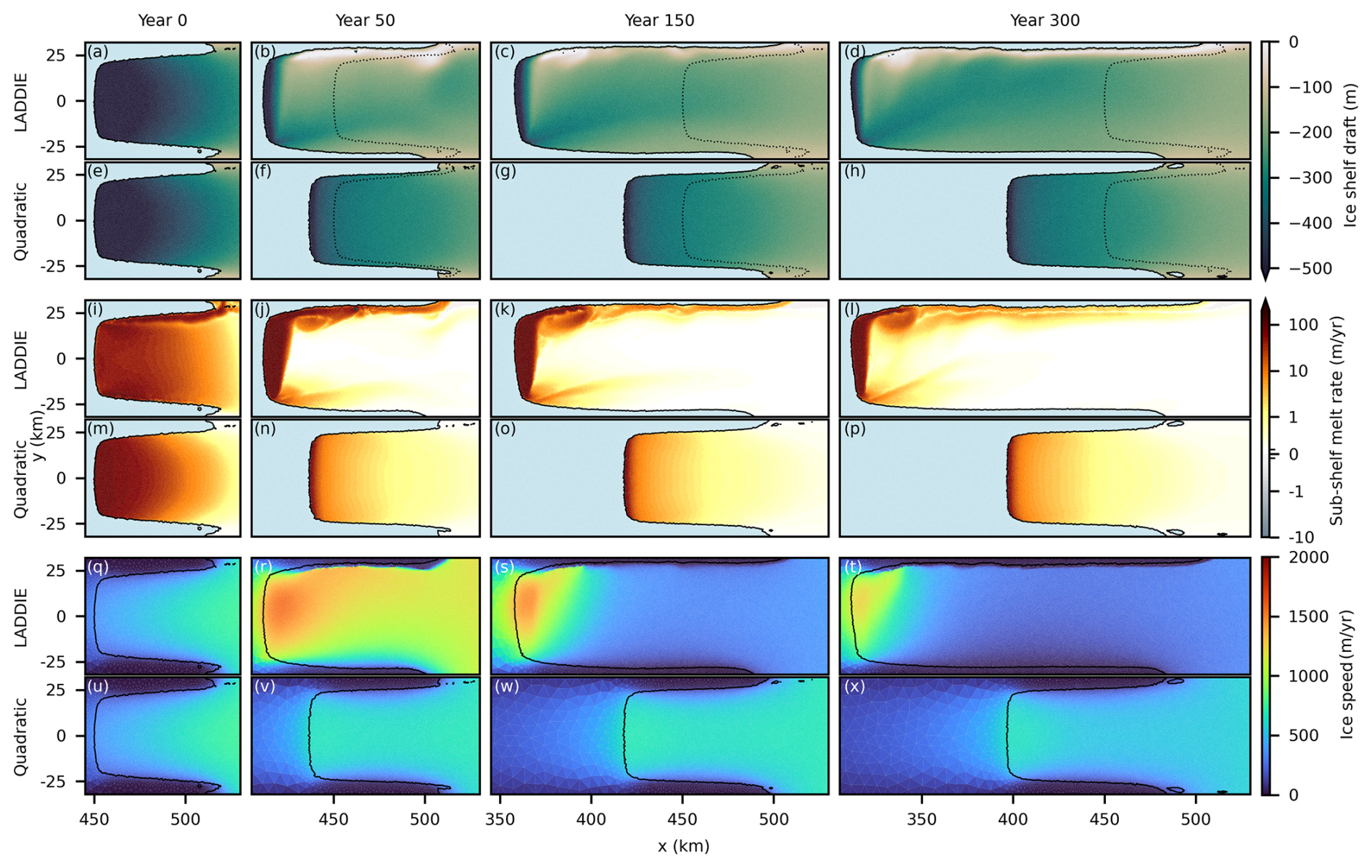
Figure 9 Ice–ocean interactions from UFEMISM comparing LADDIE to the quadratic parameterisation. The columns show four time slices of two idealised MISOMIP+ simulations. Three combined rows show the ice shelf draft (a–h), the sub-shelf melt rate (i–p), and the ice speed (q–x). For each combined row, the top row shows the LADDIE simulation, the bottom row the simulation with the quadratic melt parameterisation. Solid black lines represent the grounding line position, the dotted black lines (b–d and f–h) show the initial grounding line position (a, e).

The coupled response of an ice sheet model with LADDIE in the MISOMIP+ configuration was extensively discussed by Jesse et al. (2025), who coupled v1.0 to the ice sheet model IMAU-ICE. In agreement with that study, we see that the melt pattern by v2.0 deviates significantly from the quadratic melt parameterisation, due to the representation of the meltwater flow. First, an ocean flow establishes along the steep basal topography, facilitating strong melting not only in the deepest region, but also along the slope in shallower regions. Second, the boundary current allows for strong melting along the entire shear margin, leading to near-melt through along this boundary. These topographically induced melt patterns are in agreement with 3D ocean models (Sect. 3.2.1). With LADDIE, in contrast to the quadratic parameterisation, ice shelf thinning thus induces a partial positive feedback. Both melt enhancements along the steep slope and along the “western” boundary amplify the reduction in buttressing. This in turn allows for substantially higher ice velocities compared to the simulation with quadratic melting.

Quantitatively, the basal mass balance with LADDIE remains two to three times stronger than with the quadratic parameterisation, despite the nearly identical initial melt rates (Fig. 10). This difference is larger than the difference between LADDIE 1.0 and the quadratic parameterisation for IMAU-ICE (Jesse et al., 2025). Also the difference in grounding line retreat (1.5 times larger with LADDIE) and volume above floatation loss (2 times larger) was smaller with IMAU-ICE. The quantitative differences between these studies can be attributed to the different ice sheet dynamics of the ice sheet models, rather than the differences between version 1.0 and 2.0 of LADDIE. Specifically, these integrated UFEMISM–LADDIE simulations illustrate that the impact of 2D sub-shelf melt patterns may be larger than previously documented and dependent on the ice sheet model.

The basal mass balance in the UFEMISM–LADDIE simulation (Fig. 10a) displays a significant temporal variability. This variability is primarily induced by intermittent opening and closing of holes in the ice shelf along the high-melt boundary current. As explained in detail by Jesse et al. (2025), sub-shelf melt rates can be strong enough to melt through the ice shelf and create a hole. This hole creates a new calving front for melt plumes to exit the cavity, thereby minimising the melt rates further downstream and suppressing the integrated basal mass balance. Ice advection can close this hole, recreating an intact boundary region that allows the formation of a new boundary current with strong melting, which again can melt through and open a new hole. We have not seen evidence of melt variability related to discrete grounding line retreat, as documented by Zhao et al. (2022), which originates when high-resolution ice sheet models are coupled to coarser resolution ocean models on a regular grid. The fact that LADDIE and UFEMISM are run on the exact same mesh likely minimises this effect, and the unstructured mesh on itself may be less prone to inducing such variability than a regular squared grid.

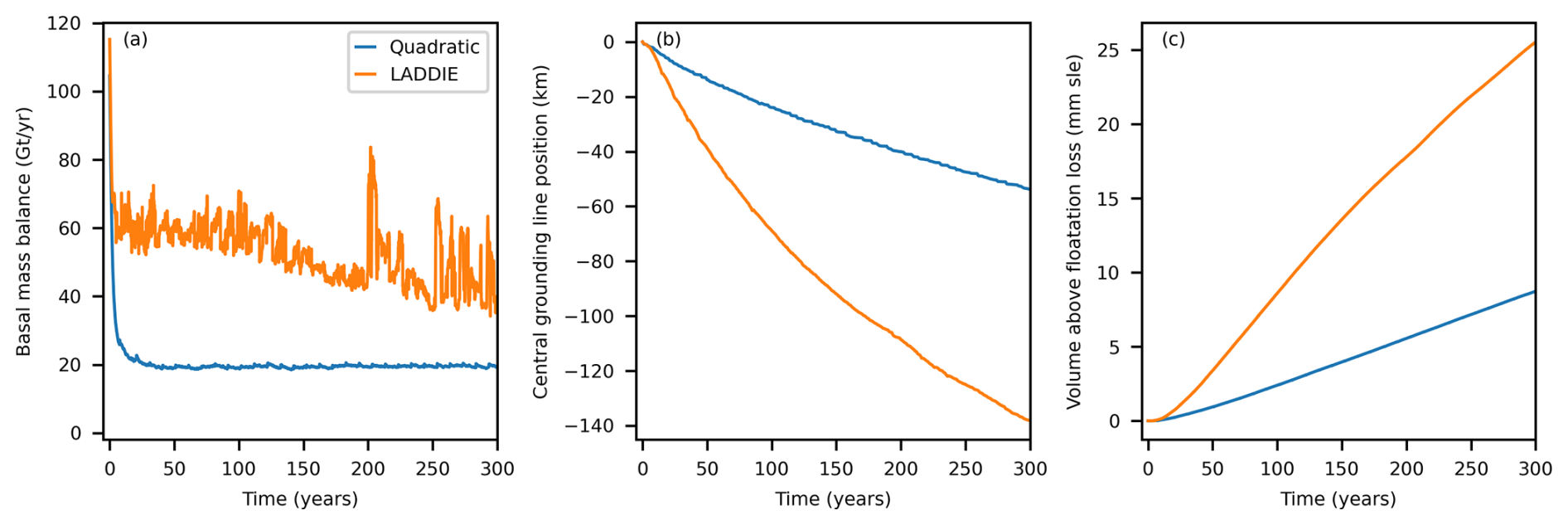
Figure 10 Time series of the two MISOMIP+ simulations. (a) The integrated basal mass balance over the whole ice shelf. (b) The grounding line position at y= 0 km, relative to the initial position at x= 450 km. (c) The volume above floatation loss.

5 Discussion

In this study, we have performed the first extensive evaluation of the 2D melt model LADDIE to both 3D ocean models and satellite-derived melt estimates. This evaluation revealed several biases, most prominently the sub-shelf melting of the George VI ice shelf in the Bellingshausen Sea. As mentioned in Sect. 3.2, preliminary tests with forcing based on Zhou et al. (2025) revealed a significant reduction in this bias. In contrast, this updated forcing contains significantly warmer ocean conditions at the Totten ice shelf, creating a new bias. These examples highlight the dependency of LADDIE to representative ocean forcing. These oceanic regions are likely subject to strong interannual variability, as is shown in the Amundsen Sea region (Dutrieux et al., 2014; Jenkins et al., 2018). Yet forcing products such as those in ISMIP6 (Jourdain et al., 2020) rely on scarce measurements in most regions, which may not cover the full range of interannual variability. Here, we choose to reveal the resultant biases in melt rates, rather than applying regional temperature corrections to obtain melt rates which better match observations, which is common practice for sub-shelf melt parameterisations (Reese et al., 2018a; Jourdain et al., 2020). These biases and their dependence on the applied ocean forcing show that a robust evaluation of any sub-shelf melt model relies on the availability of long-term, widespread, continuous in-situ ocean observations.

The evaluation to ocean models was done on steady state melt fields. Insufficient observations prevent the evaluation of interannual variability. However, we can already anticipate one discrepancy between LADDIE and 3D ocean models: the adjustment time scale. The model domain of LADDIE is limited to the upper mixed layer, which represents only a fraction of the total ice shelf cavity volume. As a consequence, the LADDIE model domain equilibrates relatively quickly. This introduces a benefit of requiring only short simulations to achieve a steady state, saving computation time. However, these adjustment time scales are a general problem in the forcing of stand-alone ice sheet models, where offshore ocean conditions are extrapolated into cavities without temporal delay (e.g., Jourdain et al., 2020). Compared to melt parameterisations, however, LADDIE has a finite adjustment timescale, which introduces some delay in the melt response to changing ocean conditions. More generally, the connection between the open ocean and ice shelf cavities is just one example of oceanic processes that models of intermediate complexity like LADDIE struggle to reproduce. Hence, it is important to stress that 2D melt models cannot replace 3D ocean models.

One key uncertainty in Antarctic ice sheet projections is the thermal melt sensitivity (Beckmann et al., 2025). In an idealised forcing assessment, the melt sensitivities of various parameterisations, LADDIE 1.0, and a Neural Network were compared (Lambert and Burgard, 2025). The conclusion was that LADDIE melt sensitivities fall within a wide range spanned by commonly used parameterisations. Yet the question what a realistic sensitivity should be remains unanswered. The inter-model comparison of RISE (Galton-Fenzi et al., 2025) sheds some light on this. We find that the thermal sensitivity of LADDIE matches closely to the multi-model mean of 9 ocean models. The thermodynamic sensitivity is higher than the multi-model mean, but close to the median value. This provides confidence that LADDIE appropriately represents the dominant underlying physical processes governing melt sensitivities. This implies that 2D melt modelling can be a pathway to reducing the large uncertainty related to melt sensitivities in stand-alone ice sheet modelling studies.

LADDIE 2.0 is written and maintained within the Utrecht Polar SYstem (UPSY) repository to optimise its integration with the UFEMISM ice sheet model. However, we have ensured that LADDIE remains a stand-alone model as well. We hope that this allows for flexible usage in both local, high resolution studies, as well as possible coupling to other ice sheet models. We foresee that minor code changes will be necessary to facilitate the wider applications of LADDIE in other modelling systems, and will attempt to implement these upon request from any user groups. That being said, we wish to stress that pan-Antarctic coupled simulations still pose several challenges compared to parameterised melting. These are primarily related to the inherent numerical nature of LADDIE, and the associated additional computational costs of running it in a coupled configuration. We plan to address these challenges in future work.

6 Conclusions

We have here presented and evaluated version 2.0 of the 2D sub-shelf melt model LADDIE. This new model version is parallellised, allowing a reduction in computation time of one order of magnitude, when configured at approximately 32 or 64 cores. Additionally, the model is written on an unstructured mesh, allowing for refinement in regions of interest.

In this study, we have provided a first extensive evaluation of the 2D sub-shelf melt model to both 3D ocean models and remote sensing estimates. In an idealised setting, LADDIE closely reproduces the multi-model mean melt pattern of 12 ocean models. In a pan-Antarctic configuration at 2 km resolution, sub-shelf melt rates and patterns agree well with both ocean models and satellite products, with regional biases likely resulting from the scarcity of available ocean observations to force LADDIE. Melt sensitivities derived from ocean models were also closely reproduced by LADDIE. At an approximate 100 m resolution, LADDIE qualitatively reproduces the channelised sub-shelf melting as mapped by remote sensing estimates.

As a use case for coupled simulations, we provide an idealised example with the ice sheet model UFEMISM, within which LADDIE 2.0 is fully integrated. In agreement with previous studies, the coupled system allows for a qualitatively and quantitatively different ice dynamical response to ocean warming, compared to parameterised melting. We hope that the availability of this open-source model can contribute to the evolution toward more robust and realistic stand-alone ice sheet modelling in future intercomparison studies such as ISMIP7 and beyond.

Appendix A: Resolution sensitivity

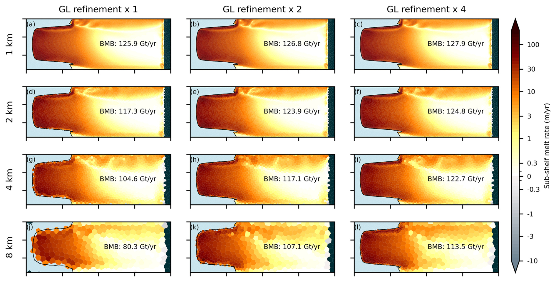
Figure A1 Sensitivity analysis to resolution over the ice shelf and refinement at the grounding line. The ISOMIP+ simulation of Sect. 3.2.1 was redone for four ice shelf resolutions (rows) and three refinement factors along the grounding line (columns). For each resolution, the integrated melt rate is expressed in Gt yr⁻¹.

To assess the sensitivity of melt rates with LADDIE to (spatially variable) resolution, we performed a sensitivity analysis (Fig. A1). In the left column, a uniform resolution requirement is applied over the ice shelf, ranging from 1 to 8 km. We see that coarser simulations produce lower melt rates, in particular along the grounding line and in the boundary current.

A refinement of the resolution along the grounding line of a factor 2 (center column) or a factor 4 (rightmost column) leads to a monotonous increase in melt rates. Strikingly, the total melt rate appears to be primarily controlled by the resolution along the grounding line. In panels a, e, and i, the resolution is a maximum 1 km, and the total melt rates vary by only a few percent. The same holds for panels b and f (both 0.5 km at the grounding line), for panels d, h, and j (2 km), and for panels g and k (4 km).

This sensitivity test illustrates the benefit of an unstructured mesh for purposes of sub-shelf melt modelling. A low resolution over the ice shelf interior, away from the grounding line, has a small impact on melt rates. Note that this may not hold for complex channelised geometries like Pine Island ice shelf (Sect. 3.3.2).

Additionally, this sensitivity test implies that melt rates seem to converge for grounding line resolutions below 1–2 km. For this idealised domain, this seems to be an approximate threshold for the geometry to robustly resolve melt rates. Notably, this is in agreement with the 2 km indication by McCormack et al. (2024). This result also confirms the importance of the model improvement from LADDIE 1.0 to LADDIE 2.0 which now allow for pan-Antarctic simulations at 2 km resolution.