
the Creative Commons Attribution 4.0 License.
the Creative Commons Attribution 4.0 License.
 | 28 Sep 2026
The NASA-GISS ModelE2.1-CC2 ESM: development and evaluation
Anastasia Romanou

Paul Lerner
Joy Romanski
Nancy Y. Kiang
Igor Aleinov
Maxwell Kelley
Ron L. Miller
Gary Russell
Reto Ruedy
Gavin A. Schmidt
Maria Z. Hakuba
This paper describes the NASA Goddard Institute for Space Studies (GISS) ModelE2.1-Carbon Cycle version 2 Earth System Model (NASA GISS E2.1-CC2 ESM), assesses its skill against observations and the previous version of the same model (GISS‐E2.1‐G‐CC). NASA GISS E2.1-CC2 ESM includes the same physical climate model E2.1-G as its predecessor, updated ocean and land carbon cycle and longer equilibrium simulations. While the focus here is on the land and ocean carbon components and their interactions with the atmosphere and ice, we also describe in detail the physical coupled model for consistency and ease of reference. We detail parameterizations, tuning, and conservation diagnostics that are relevant to the global (land and ocean) carbon cycle. We also describe the pre-industrial control and the historical simulations with this model while future climate scenarios will be addressed in a companion paper. The model is an improvement to prior releases, has been better tuned and spun up (all reservoirs: the ocean, the ocean carbon but especially the soil carbon reservoir) and exhibits smaller drifts in all carbon components. However, some persistent biases remain, particularly with regards to low ocean productivity and land primary production. Low ocean productivity may be due to (i) low iron concentration in high-nutrient and low chlorophyll regions, and (ii) lack of photoadaptation, which would increase the ratio in low-light environments, relieving light limitation beneath the surface of the ocean. Low land productivity may result from an insufficient gross primary productivity increase due to lack of prognostic LAI, or drought stress, or an underestimated CO2 fertilization effect, or an overestimate of soil respiration due to biases in soil moisture, soil temperature, and/or how soil respiration responds to these environmental variables.
- Article
(16991 KB) - Full-text XML
-
Supplement
(8513 KB) - BibTeX
- EndNote


Earth system models (ESMs) integrate the interactions of atmosphere, ocean, land and ice with the biosphere to estimate the state of regional and global climate under a wide variety of conditions (Heavens et al., 2013) and focus on comprehensiveness of Earth system interactions, feedbacks and interdependencies. ESMs include all the processes present in climate models, but they also simulate the interaction between the physical climate, the biosphere and the chemical constituents of the atmosphere and the ocean. They can also include the impact of human decision-making, e.g. changes in land use, in emissions mitigation etc. They are thus particularly useful for estimating remaining carbon budgets before anthropogenic warming exceeds certain thresholds, studying the feasibility, scalability and impacts of climate intervention practices and geoengineering activities, such as carbon dioxide removal (CDR) through soil carbon sequestration, biomass carbon removal and storage, enhanced mineralization, ocean alkalinity enhancement, afforestation/reforestation etc and studies of the Earth's climate evolution after curbing emissions.
The NASA Goddard Institute for Space Studies (NASA-GISS) ModelE version 2.1 with Carbon Cycle version 2 (ModelE2.1-CC2) is an Earth system model with a fully interactive land and ocean carbon cycle which is an update of the GISS submission to the 6th generation Climate Model Intercomparison Project (CMIP6) which was identified as GISS-E2-1-CC in the CMIP6 repository. We will use the shorthand GISS-ESM CMIP6+ alternatively with GISS-E2-1-CC2 to denote the difference from the previous model.
In the following sections we describe as comprehensively as possible the physical and biogeochemical components of the model, the relevant parts of the radiation, atmospheric chemistry and clouds. We then present results from the spinups and historical simulations and assess them against observations. Lastly, we lay out the model response to future emission and mitigation pathways. Lastly, we offer a summary of the model, comparison with other models across different experiments in the post-CMIP6 assessments and lay out our future modeling plans.
The underlying physical model, ModelE2.1, has been described in Kelley et al. (2020) and includes updates to earlier versions of the NASA GISS model (Schmidt et al., 2006; Hansen et al., 2007; Schmidt et al., 2014). For ease of access and comprehensiveness of model presentation, we will describe key components of the model here as well, although complete information and evaluations of the physical model should be sought in these publications.
2.1 Model configuration
The atmospheric model has horizontal resolution of 2 by 2.5° in latitude and longitude respectively and 40 layers in the vertical from the surface to 0.1 hPa in the lower mesosphere; it is coupled to an ocean with 1 by 1.25 horizontal resolution in latitude and longitude respectively and has also 40 layers in the vertical.
Atmospheric dynamics uses Arakawa's B-grid scheme where eastward and northward velocity components are located at primary cell corners; vertical discretization follows terrain‐following (sigma) layers in the troposphere which transition to constant‐pressure layers in the stratosphere. The transition is smooth and centered at 100 hPa with a half‐width of approximately 30 hPa. The vertical discretization in the ocean is 40 vertical layers in mass with higher resolution of 5–20 m near the surface and within the thermocline and about 200 m at depth.
Prognostic variables in the atmosphere are dry air mass, potential temperature, water vapor mixing ratio, and horizontal velocity components. Virtual potential temperature is used for all density/buoyancy-related calculations. Ocean prognostic variables include seawater mass, potential enthalpy that accounts for variations in specific heat capacity, salt and horizontal velocity components on both the C-grid (perpendicular to primary cell edges) and D-grid (parallel to primary cell edges).
Subsurface reservoirs are split into four types: open water (including lakes and oceans), ice-covered water (including lake ice and sea ice), ground (including bare soil and vegetated regions), and land ice/glaciers. Within each type there are further subdivisions (fraction of plant functional types, fractional snow cover, melt pond fraction over sea ice, etc.), which are communicated to the atmospheric model as weighted mean quantities (for example the albedo in the radiation computations). The non-ocean reservoirs include prognostic variables for water mass and heat content, and the sea ice also includes salt content.
The model uses a 30 min time step for physics calculations (i.e. surface interactions, condensation etc). The radiation code is called every five physics time steps (every 2.5 h), however, the zenith angle and sun light intensity are updated every physics time step. The model uses a 225 s time step for the atmospheric dynamics (transports) and 112.5 s time step for ocean gravity wave computations.
Simplifications in atmospheric thermodynamics ignore the sensible heat of condensate. Although latent heat of water vapor is treated correctly, its mass is not added to atmospheric dry mass. Consequently, precipitation and evaporation occur at 0 °C, specific potential enthalpy equals potential temperature times dry specific heat capacity, and humidity affects atmospheric density only in the pressure gradient force computation.
2.2 The ocean component
The ocean model is a dynamic ocean model E2.1-G (Russell et al., 1995; Schmidt et al., 2006, 2014; Kelley et al., 2020), non-Boussinesq (i.e. includes density variations in the horizontal as well as vertical momentum equations and in the continuity equation, following Schmidt et al., 2006). It conserves potential enthalpy, freshwater mass, and salt mass, and uses natural boundary conditions (for heat and freshwater). It has a free surface and thus it is not volume conserving. The number of vertical layers varies from 2 to 40. After the dynamics, the mass ratio of layer n and its layer above is fixed in time and space, but this does vary with n. The thickness of layer 1 varies and is approximately 10 m. The vertical coordinate is mass per unit area, including the mass of air, ice and water above any level.
The ocean model solves the dynamical equations via an invariant form. The Coriolis term is computed via the C and D-grid velocities and has latitude dependence. The quadratic upstream advection scheme (Prather, 1986) uses mean, three-dimensional gradients, and second order moments to advect scalar tracers, thus effectively increasing the resolution, in both horizontal and vertical direction. Bottom friction is applied at the lowest layer of each ocean column. The ocean model employs the K-profile parameterization (KPP) for vertical mixing (Large et al., 1994) and the Gent-McWilliams parameterization for eddy induced tracer transports (Griffies, 1998a, b). The mesoscale diffusivity allows for surface‐intensified eddies, by employing an exponential decay of diffusivity with depth that depends locally on the horizontal gradient of potential density (Kelley et al., 2020) which permits eddies to restratify the Southern Ocean over a large depth range, consistent with the observed density structure there, while not overacting in other regions of the World Ocean (such as the North Atlantic). The Rossby radius is replaced by a geographically constant nominal length scale, and the diffusivity is a function of the Brunt‐Vaisala frequency and the slope of isopycnal surfaces.
Mesoscale transport is expressed in local quasi‐isopycnal layers, avoiding difficulties associated with skew-flux representation (1) in regions with weak vertical stratification, e.g. the surface mixed layer and at the ocean surface, where the GM parameterization assumes that eddies transport tracers along isopycnal surfaces. However, near the surface, these surfaces can be highly tilted or intersect the ocean surface, which violates the assumptions of the parameterization. Applying the GM scheme directly in these regions can lead to spurious mixing and incorrect representation of processes like deep convection and mixed-layer re-stratification, (2) near lateral boundaries and the ocean bottom, where the eddy fluxes must be parallel to these boundaries, but the GM scheme's isopycnal-following nature doesn't naturally enforce this, and (3) in areas of strong density fronts (e.g., the Gulf Stream or the Antarctic Circumpolar Current) where the “small-slope approximation” which assumes that the slope of isopycnal surfaces is small and is valid in the deep ocean, breaks down in areas where the isopycnals are steeply tilted. Ventilation of marginal seas through their connecting straits has been increased via two mechanisms in E2.1‐G, reducing salinity biases there. While there is no explicit overflow parameterization in the ocean model, for straits deep enough that density contrasts can drive strong opposing flows at the surface and at depth, the finer upper‐ocean layering in E2.1‐G resolves this structure, in conjunction with a slight tuning of strait depths. Second, horizontal diffusivity was increased in straits that are shallow or have weaker density contrasts. The first mechanism impacted the Red and Black seas, and the second the Baltic and Hudson (Kelley et al., 2020). The first is the sole ventilation mechanism for straits narrower than the nominal resolution, which are parameterized using the Russell et al. (1995) one‐dimensional channel scheme that lacks horizontal mixing.
In addition to KPP, the vertical diffusivity also includes a contribution from tidal dissipation. The ocean model Atlantic meridional overturning circulation (AMOC) is found to be sensitive to tidally driven mixing, which occurs in the shallow waters bordering the North Atlantic following dissipation distributions generated by Jayne (2009).
The Equation of State employed in the ocean model computes specific volume (m3 kg−1) as a function of specific potential enthalpy (J kg−1), salinity (psu), and pressure (Pa). Using constant uniform gravity, pressure at any level is gravity times mass per unit area above the level. The one-to-one relationship between temperature and specific potential enthalpy is computed using the adiabatic lapse rate of sea water as function of temperature, salinity and pressure (IES-1980 et al., 1981) and specific enthalpy of sea water as function of temperature and salinity at atmospheric pressure. Using these formulas, the model's Equation of State can be computed from the specific volume function of temperature, salinity and pressure (IES-1980 et al., 1981). Complex computations for Equation of State, freezing temperature, specific heat capacity, and others are evaluated offline and are stored in tables; the model interpolates the table values as functions of specific potential enthalpy, salinity and pressure (Chen and Millero, 1976). Table resolutions are 4000 J kg−1 of specific potential enthalpy, 1 psu of salinity, and 2×10⁶ Pa of pressure. Under adiabatic flow, potential enthalpy is a conserved quantity, therefore the ocean model conserves energy (heat) as well as mass and salt.
2.2.1 Ocean Carbon Cycle
The ocean carbon cycle model is based on the NASA Ocean Biogeochemistry Model (NOBM), originally developed at the NASA-Global Modeling and Assimilation Office (Gregg and Casey 2007) and later coupled coupled to the GISS climate model under prescribed atmospheric concentrations (Romanou et al., 2013, 2014) and under prescribed emissions (Ito et al., 2020). The model includes four phytoplankton species (diatoms, chlorophytes, cyanobacteria, and coccolithophores), four nutrient species (nitrate, silicate, ammonia, and iron), three detrital pools (nitrate/carbon, silicate, and iron) and one heterotroph species (Fig. 1). Carbon cycling is represented through dissolved organic (DOC) and inorganic carbon (DIC), where carbonate chemistry is solved using MOCSY (Orr and Epitalon, 2015). Ocean carbon interacts with atmospheric CO2 through gas exchange parameterization, following the CMIP6 protocol (Orr et al., 2017). The current version of NOBM (NOBMg) has been expanded to include oxygen and alkalinity (Lerner et al., 2021, 2024) and an updated treatment of iron scavenging (see below). The model equations and parameters used are laid out in Appendix A and in Tables A1–A11 therein. A short description of the model equations is provided below.
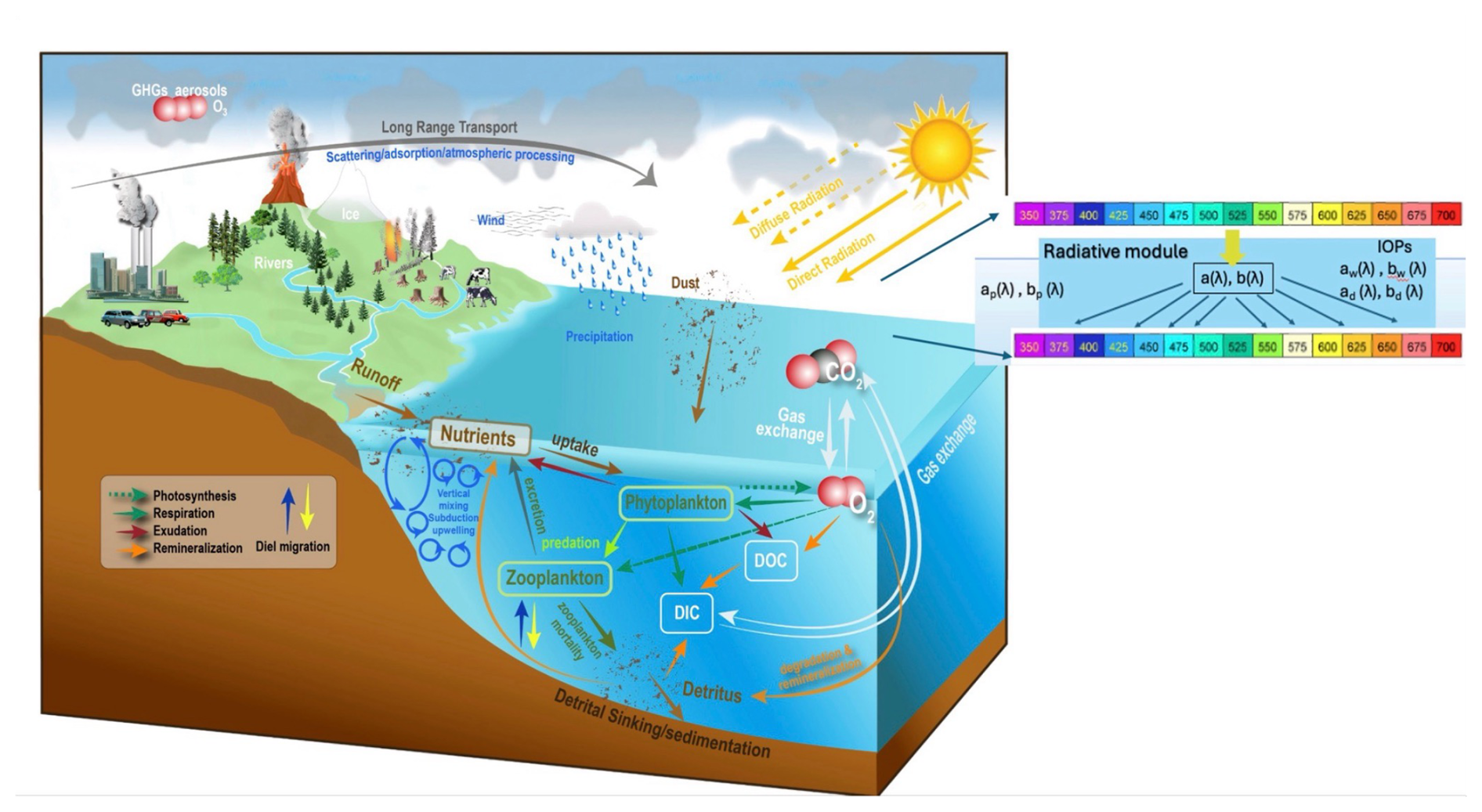
Figure 1Schematic diagram of the ocean carbon cycle model (NOBMg). credit: Jay Friedlander, NASA-GSFC.
All tracers in NOBMg are changed via physical transport and mixing which are following parameterizations of these processes in the physical ocean model.
Phytoplankton species are also subject to sinking, growth via nutrient uptake, respiration and exudation of DOC, senescence and zooplankton grazing. Nutrient distributions are changed via uptake by phytoplankton species for growth, remineralization of particulate organic carbon or nitrogen, and detrital breakdown. Cyanobacteria can also grow via nitrogen fixation, where growth is limited only by light, iron, and temperature. Nitrogen assimilated into organic matter is obtained from N2. Cyanobacterial growth via nitrogen fixation follows the same Michaelis-Menten formulation as cyanobacterial growth that is nitrate limited, with two exceptions. First, the iron half-saturation constant for nitrogen fixation is 33 % higher than that for nitrate-limited growth, as nitrogen fixation generally relies upon an increased availability of iron. Second, nitrogen fixation is inhibited by the presence of nitrate and ammonium, following laboratory culture experiments using Trichodesmium (Holl and Montoya, 2005). Ammonium is produced via the herbivore grazing and heterotrophic loss. Silicate is taken up only by diatoms. Iron is produced by zooplankton, atmospheric deposition of dust, and is lost to scavenging. NOBMg also includes an updated marine iron cycle, with regionally varying prescribed ligands, and a significant increase in the rate of ligand-bound iron scavenging, to be consistent with observed rates for trace metals with similar scavenging characteristics as iron (see Sect. 3.1.1 on Tunings). At each time step, the prognostic iron pool is split into iron that is complexed by organic ligands and a “free” iron pool that represents the sum of all inorganic iron species. Iron complexation chemistry is computed at each time step using vertical and regionally varying prescribed ligand concentrations (see Sect. 3.1.2 Forcings) and a conditional stability constant (KFeL) = 1011 L mol−1. Then, free and ligand-complexed iron are computed by solving the system of equations for total iron, total ligand concentration, and the conditional stability constant (Aumont et al., 2015).
Herbivores grow via grazing of phytoplankton and are lost to heterotrophic consumption and excretion to DOC.
Carbon and nitrate particulates (detritus) are linked via the constant C:N ratio. Therefore, only one equation is used to describe both. Their change is due to advection and diffusion, sinking, remineralization and detrital breakdown. Sinking of particulates is expressed via an exponential function of depth (see Eqs. A15–A17). Silicate detritus includes an additional source term due to senescence of phytoplankton and grazing from herbivores. The iron detritus includes zooplankton production and scavenging production. DOC is produced during phytoplankton growth, herbivore excretion and detrital breakdown while the only DOC sink is bacterial degradation. DIC sources are phytoplankton and herbivore respiration, bacterial degradation of DOC, remineralization of carbon detritus and air sea exchange while the only sink is the growth of phytoplankton.
The model includes prognostic alkalinity which is advected and mixed like all other tracers and follows the Ocean Carbon Model Intercomparison Project parameterizations (OCMIP-2, Najjar et al., 2007), i.e. it is produced via conversion of nitrate to organic N and carbonate dissolution, while it is lost to remineralization of detrital organic carbon nitrogen and DOC and carbonate precipitation (see Eqs. A43–A47).
Oxygen interacts with the rest of the ocean biogeochemical tracers via remineralization of organic carbon and by determining when the model switches to slower rates of remineralization that are consistent with denitrification (Eqs. A48–A56; Lerner et al., 2024).
2.3 The Land component
2.3.1 Vegetation
The Ent Terrestrial Biosphere Model (Ent TBM) (https://www.giss.nasa.gov/projects/ent/, last access: 21 August 2026) is a demographic dynamic global vegetation model (DGVM) (Kiang, et al., 2006; Kim et al., 2015) with subgrid vegetation patches distinguished by plant functional type (PFT), currently with single-cohort structure for patch communities (Fig. 2). The 12 plant functional types are: evergreen broadleaf trees, evergreen needleleaf trees, cold deciduous broadleaf trees, drought deciduous broadleaf trees, deciduous needleleaf trees, cold-adapted shrubs, arid-adapted shrubs, C3 perennial grass, C3 annual grass, C3 arctic grass, C4 grass, and herb crops (with physics of C3 perennial grass). Soil biogeochemistry is a version of the Carnegie-Stanford-Ames' (CASA') model (Potter et al., 1996; Randerson et al., 2009; Doney et al., 2006), modified for Ent for an improved response of soil respiration to soil moisture, as described in Kim et al. (2015). Land ecosystem carbon pools that are calculated are: foliage, hardwood stem, sapwood stem, fine roots, coarse roots, non-structural carbohydrate (which we also call labile carbon), and 9 soil carbon pools.
Leaf biophysics is a coupled conductance/photosynthesis model that simulates vegetation stomatal control of both transpiration and uptake of CO2. The coupled leaf photosynthesis/ stomatal conductance model consists of the photosynthesis model of Farquhar and von Caemmerer (1982) and the Ball-Berry model of stomatal conductance (Ball and Berry, 1987), with leaf boundary layer conductances following the approach by Collatz et al. (1991) but with the boundary layer conductance derived from the canopy surface layer conductance of the land surface model; for the cubic equations of coupled photosynthesis/conductance, a numerical solver for net assimilation of CO2 and leaf internal CO2 concentration was developed. C4 photosynthesis follows the scheme of Collatz and Berry (1992). Leaf-to-canopy scaling is achieved through the canopy radiative transfer scheme of Spitters et al. (1986) (introduced to ModelE in CMIP5 in Schmidt et al., 2006) combined with a numerical scheme for vertical layering of the canopy by converging the total canopy fluxes. Vegetation canopy absorbance and transmittance of photosynthetically active radiation thus depend on vertical layering of leaf area index, solar zenith angle, and the fractions of diffuse vs. direct radiation, providing vertical profiles of sunlit and shaded leaf area fractions. Physiological algorithms for water stress, cold hardening in evergreen needleleaf trees, and temperature sensitivity of photosynthetic capacity are detailed in Kim et al. (2015). To account for variation in parameters of the leaf biophysics by climate and seasonality of vegetation, temperature dependence of leaf photosynthetic capacity, Vcmax, is modeled with a Q10 function (Hegarty, 1973), with a reference temperature of 25 °C and parameters from Collatz et al. (1991). In addition, photosynthetic capacity is subject to seasonal cold hardening in evergreen needleleaf trees, as a function of local air temperature trend, and is modeled based on the work of Repo et al. (1990); Hanninen and Kramer (2007); and Makela et al. (2004, 2006). Autotrophic maintenance respiration is subject to temperature acclimation, in which the reference optimal temperature in the equation of Levis et al. (2004) is allowed to vary between 10–30 °C, tracking a 10 d running average of surface air temperature; 10 d averages less than 10 °C or greater than 30 °C are considered outside the range of acclimation.
Water stress is modeled after the approach of Rodriguez-Iturbe et al. (2001), in which stress is a factor between 0 (full stress) and 1 (unstressed), as a function of relative extractable water (volume water − minus hygroscopic water)(pore volume minus hygroscopic water). The factor modifies the leaf stomatal conductance, and different plant functional types have different critical soil moisture values for the onset of stress and wilting points. Because transpiration depends on the exposed leaf area index, and wet leaf fractions will not transpire, a scheme for canopy interception of precipitation was added following the algorithm presented in Koster and Suarez (1996) which is like the modified Shuttleworth scheme of Wang et al. (2007). The scheme primarily involves modification of the wet fraction of the canopy by computing the drip rate considering the fraction of precipitation that falls onto a previously wetted portion of the canopy with the grid cell. This scheme also distinguishes between stratiform and convective precipitation, because the stratiform type covers a greater portion of the grid cell than the convective type (e.g., Koster and Suarez, 1996; Wang et al., 2007).
For surface albedo, Ent's 12 different vegetation types have different spectral and snow masking depth properties. In E2.1 Ent PFTs are mapped to the 8 biome types of Matthews (1984) for seasonal albedo for radiative purposes.
In Schmidt et al. (2006) and henceforth, all surface conductance of water vapor for vegetated land was assigned to the vegetation, which meant that there was no soil evaporation under canopies. The rationale for this approach (Abramopoulos et al., 1988) was that vegetated land was simply a surface with a particular albedo and conductance. Numerous studies have demonstrated the importance of soil evaporation as a component of evapotranspiration, especially for semiarid ecosystems (e.g., Lawrence et al., 2007). While evaporation from bare soil was included in previous versions of the model, in E2.1 we have added a simple representation of soil evaporation based on the work of Zeng et al. (2005) and Lawrence et al. (2007), by including the evaporative flux from the vegetated soil into the total evapotranspiration scaled as a function of the current leaf area index. Total evapotranspiration never exceeds the potential evaporation.
2.3.2 Irrigation and Groundwater
In E2.1, irrigation is implemented as a prognostic field (Cook et al., 2011, 2014; Krakauer et al., 2016; Puma and Cook, 2010; Shukla et al., 2014) where water demand for irrigation (Wada et al., 2014) is estimated using prescribed irrigation areal extent (Siebert et al., 2015). The water is drawn first from rivers and lakes locally, and if that is insufficient, it is drawn from an external groundwater source (which is tracked diagnostically). Groundwater is assumed to have the same temperature as the soil and default tracer concentrations. Groundwater recharge is not accounted for, and so there is a small increase in total water mass (and eventually, sea level) associated with the net global groundwater draw in these simulations. These effects have a complex impact on freshwater delivery to the oceans (and hence sea level). Irrigation from local surface water sources leads to increased soil moisture and reduced river outflow, but this is dominated by net additions of groundwater which add freshwater to the climate system, about 0.2 mm yr−1 of global sea-level-equivalent in 2010 (Miller et al., 2021). As discussed in Miller et al. (2021) this freshwater imbalance is driven by an underestimate of surface water in lakes and rivers (which means that more groundwater is needed) and also the lack of counteracting increase in reservoirs.
2.3.3 The Land Carbon Coupling
The land carbon dynamics in the fully coupled carbon cycle physics configuration is the same as described in Ito et al. (2020) for the ModelE submission to CMIP6 C4MIP. The leaf biophysics is sensitive to the surface atmospheric CO2 concentration. The model tracks CO2 exchanges between the land and atmosphere in diagnostics for GPP, autotrophic respiration, soil respiration, and carbon fluxes due to land cover change. Land carbon change associated with the annual land cover change is distributed as CO2 fluxes to the atmosphere over the following year to avoid having to add a pulse of CO2.
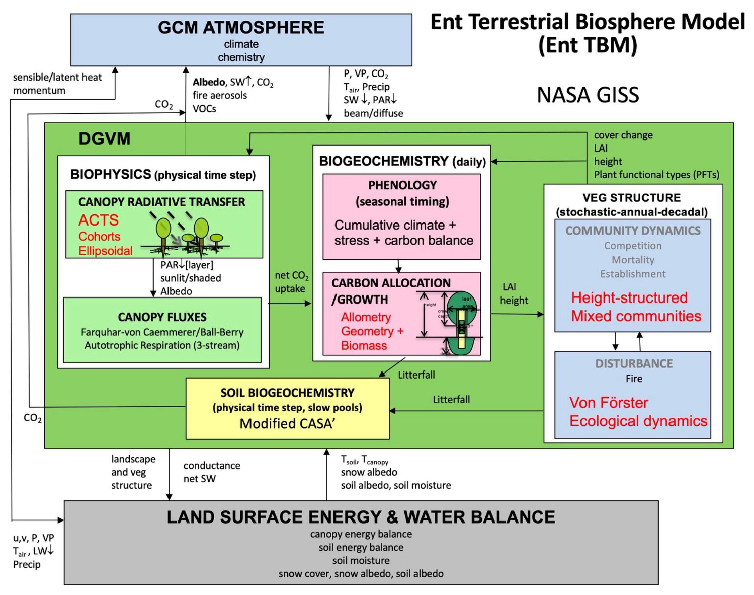
Figure 2Schematic diagram of the Ent in GISS ModelE2.1-CC2.
2.4 The sea ice and land ice models
Sea ice and lake ice are computed on the atmospheric grid, and the information is mapped on to the ocean grid. Temperature and salinity profiles in the ice are computed prognostically, and sea ice distribution trends and seasonal cycles are realistic (Kelley et al., 2020).
Salinity in the ice affects basal ice formation/melt and heat diffusion (Schmidt et al., 2006) using brine-pocket (BP) thermodynamics (Bitz and Lipscomb, 1999; Schmidt et al., 2014) and updated in Kelley et al. (2020). Sea ice dynamics use the viscous-plastic formulation of Zhang and Rothrock (2000). Lead fraction is treated differently in the Arctic and Antarctic wintertime thick-ice growth to produce more realistic heat fluxes and sea ice growth rates. Processes relevant to the salt budget (e.g., gravity drainage and flushing of meltwater) are consistently treated with the BP physics.
The mass and energy associated with net snow accumulation over each hemisphere's ice sheets is used to adjust the implicit iceberg calving fluxes into the adjacent oceans over a 10-year relaxation time, and this diagnostic is preserved as glacial melt. This ensures that the model can reach a long-term equilibrium under changed climate forcings but does not imply realism in the response of ice sheets to climate, since the ice sheets are assumed to remain in mass balance.
2.5 Radiation, Clouds and Atmospheric Composition
The total solar irradiance at the top of the model's atmosphere is based on satellite calibrations (Kopp and Lean, 2011) with a base value of 1361 W m−2. Spectral irradiance values are taken from Coddington et al. (2016). The radiation model includes explicit multiple scattering calculations for solar radiation (shortwave, SW) and explicit integrations over both the SW and thermal (longwave, LW) spectral regions (Schmidt et al., 2006; Schmidt et al., 2014; Kelley et al., 2020). SW radiation is absorbed by H2O, CO2, O3, O2, and NO2 using the k-distribution approach (Lacis and Oinas, 1991) that utilizes 15 noncontiguous spectral intervals to model overlapping cloud–aerosol and gaseous absorption and is scattered by clouds and aerosols using size-dependent Mie scattering, ray tracing and T-matrix theory (Mishchenko et al., 1996).
Longwave radiation is absorbed by H2O, CO2, and O3 using the correlated k distribution with 33 intervals (Lacis and Oinas 1991; Oinas et al., 2001), designed to match line-by-line computed fluxes and cooling rates throughout the atmosphere to within about 1 %. Weaker bands of H2O, CO2, and O3, as well as absorption by CH4, N2O, CFC-11, and CFC-12 are included in an approximate fashion as overlapping absorbers, but with coefficients tuned to reproduce line-by-line radiative forcing over a broad range of absorber amounts.
Variations in incoming solar forcing in the 20th Century simulation follow Matthes et al. (2017) and include updated spectral solar irradiance. Orbital parameters that determine the seasonal and latitudinal variation in insolation are calculated each year (updated on 1 January), based on Berger (1978).
The radiation model also includes the effects of 3D cloud heterogeneity via the 3D cloud parameterization (Cairns et al., 2000) to get more realistic albedos from realistic water paths and particle sizes (Schmidt et al., 2006). The procedure rescales optical depth, asymmetry parameter, and single scattering albedo according to the relative variance of the cloud particle density distribution. The partitioning between convective precipitation that descends and has the potential to evaporate in the environment rather than in the downdraft is increased from 0 % to 50 %, thus increasing the sensitivity of humidity to convection. The downdraft buoyancy is based on virtual temperature including condensate loading. Glaciation in the mixed‐phase temperature range has been updated in the stratiform cloud parameterization.
Stratiform cloud formation is done more realistically because there is no restriction in coverage, no dependence on vertical motion, the altitude is taken to be relative to local planetary boundary layer (PBL) height rather than a fixed 850 hPa, better demarcating cloud‐topped boundary layers from the free troposphere where the threshold relative humidity is used for the TOA radiation balancing process (described in Sect. 3.1.1) to maintain top‐of‐the‐atmosphere radiative balance.
The advection of humidity (and other tracers) is done only once every physics time step (30 min) with iterative time stepping to avoid any Courant–Fredrichs–Levy violations. The smaller time steps are used primarily in the stratosphere and upper troposphere where zonal winds are strong or as a result of extremely high flow deformation.
The atmospheric chemistry configuration used in GISS ModelE2.1-CC2 is the basic non-interactive composition (NINT f2 used in CMIP6) in which the background fields of ozone and aerosol concentrations (dust, sea-salt, sulfate, nitrate, ammonium and carbonaceous aerosols e.g. black and organic carbon) are derived from simulations of the interactive one-moment aerosols (OMA) version of the model, run as an atmosphere only model with prescribed SST (Kelley et al., 2020). All anthropogenic and biomass burning emissions of short‐lived species were updated to CMIP6 specifications (Hoesly et al., 2018; van Marle et al., 2017) and were prescribed annually or monthly.
Specifically, with regards to dust, the six dust bins (0.1–0.2, 0.2–0.5, 0.5–1, 1–2, 2–4, and 4–8 µm particle diameter), are used for coatings on dust particles, the dust particle densities, and the weights that are used to partition the total clay which is advected as a bulk species in the model. The weights reflect the size distribution of dust. The effect of wind biases on dust transport over the dust source regions is alleviated in the model by employing an additional term (“gustiness”) to express the high frequency variability in the surface winds that lift dust into the atmosphere. This variability results from stirring of the atmospheric boundary layer by dry convective thermals or frictional eddies, along with downdrafts spreading outward from the base of convective events. The magnitude of the associated wind gusts is parameterized as described by Cakmur et al. (2004). The longwave optical depth for dust was increased by 30 % to account for the longwave scattering effect. The lensing effect of sulfate and nitrate coatings on BC was parameterized by increasing the shortwave optical depth for BC by 50 %. For more information see Pérez García-Pando et al. (2016).
Currently in NOBMg within GISS ModelE2.1-CC2, dust iron deposition is obtained from the historical annual cycle climatology extracted from the GISS E2.1-G online dust simulations which include eight externally mixed minerals (illite, kaolinite, smectite, carbonates, quartz, feldspar, iron oxides, and gypsum) plus internal mixtures between seven minerals and iron oxides (Perlwitz et al., 2015a; Perlwitz et al., 2015b). The masses of free and structural iron and their fractions of total iron have been evaluated using measurements from Izaña Observatory (Pérez García-Pando et al., 2016). For more on the dust deposition, see Sect. 3.1.2 on Forcings. In future versions of the model, dust deposition will be interactive with the global carbon cycle.
A second order scheme is used for the transport (Schmidt et al., 2006) of all the tracer fields in the atmosphere which are advected using the highly non-diffusive quadratic upstream scheme (QUS; Prather, 1986), which keeps track of nine subgrid-scale moments as well as the mean within each grid box. This increases the effective resolution of the tracer fields and allows the GISS model to produce reasonable climate fields with relatively coarse nominal resolution.
2.6 Surface albedo
The radiation model generates spectrally dependent direct/diffuse flux ratios for use in biosphere feedback interactions. The surface albedo utilizes six spectral intervals, in nanometers: nm: VIS (300–770), NIR1 (770–860), NIR2 (860–1250), NIR3 (1250–1500), NIR4 (1500–2200), NIR5 (2200–4000), and is solar zenith angle dependent for ocean, snow, and ice surfaces.
The spectral and solar zenith angle dependence of ocean albedo is based on calculations of Fresnel reflection from wave surface distributions as a function of wind velocity (Cox and Munk, 1956) taking also into account the effects of foam and hydrosols on ocean albedo (Gordon and Jacobs, 1977). The spectral and solar zenith angle dependence of snow and sea ice is modeled following Warren and Wiscombe (1980). Snow “ages” following Loth and Graf (1998) and has a different albedo for wet or dry snow. Ocean ice albedo is spectrally dependent and is a function of ice thickness and parameterized melt pond extent (Schmidt et al., 2006 and references therein).
Light profiles from the atmospheric radiation module are propagated underwater into the ocean and spectrally decomposed to 33 wavebands that are used to compute growth of the phytoplankton groups, sinking profiles, as well as changes in the vertical distribution of ocean temperatures due to biologically mediated absorption and scattering in the water column (Gregg and Conkright, 2002). NOBMg is coupled prognostically to the atmospheric radiation module which is part of ModelE2.1. Direct and diffuse sunlight in 6 wavebands (5 in the near IR and 1 in the visible part of the spectrum) that are computed by the radiation module are decomposed into the 33 wavelengths (250–3700 nm) needed for the absorption and scattering by the different phytoplankton species. The decomposition factors are based on the fractions of direct (diffuse) sunlight at the equator for each wavelength relative to the total radiation as derived from a monthly climatology provided by the Ocean–Atmosphere Spectral Irradiance Model (OASIM) and forced by MODIS data for aerosols and clouds (Gregg and Casey, 2007).
Vegetation spectral albedo is prescribed as seasonally varying by plant functional type (PFT) and is treated as Lambertian, assuming a flat, diffusely reflecting surface. Bare soil is represented as grey, with values from Matthews (1984). Seasonal spectral albedos for vegetation are specified by mapping Ent PFTs to the eight Matthews biome types: tundra (Ent cold-adapted shrubs), C3 grass (Ent C3 perennial, annual, and arctic grasses), shrub (Ent arid-adapted shrubs), deciduous forest (all Ent deciduous trees), evergreen needleleaf forest (Ent evergreen needleleaf trees), tropical rainforest (Ent evergreen broadleaf trees), and crops (Ent crops). Total land albedo is calculated as a weighted average across the corresponding land-cover fractions and linearly interpolated between prescribed seasonal values. When snow is present, snow albedo is included in the weighted average according to its masking fraction.
2.7 Interface exchanges
2.7.1 Surface fluxes
Separate atmospheric surface fluxes are computed for each subsurface reservoir: open water, sea or lake ice, land ice, snow free and snow-covered ground. ModelE calculates atmospheric turbulence over the entire vertical column. The surface fluxes are calculated using a submodule that is embedded between the surface and the midpoint of the first resolved model layer. In the atmospheric planetary boundary layer (PBL), a formulation for the temperature, moisture, and scalar fluxes is employed and consists of a local (diffusive) term and a countergradient term derived from large-eddy simulation (LES) data (Holtslag and Moeng, 1991) as well as a nonlocal vertical transport scheme for virtual potential temperature, specific humidity, and other scalars (Holtslag and Boville, 1993).
A level-2.5 turbulence model (Cheng et al., 2002; Yao and Cheng, 2012) is applied to this region (using eight sublayers) independently over each surface type where the mixing profile depends on the height of the PBL, which is closely related to the large eddy size and thus characterizes the nonlocality, and the buoyancy and shear effects at the surface. The turbulence length scale formulation is obtained from the large eddy simulation data by Nakanishi (2001).
Above the PBL a second-order closure (SOC) model developed by Cheng et al. (2002) is used, which is based on Mellor and Yamada (1982). The Reynolds stress and heat flux equations have been solved with a more advanced parameterization of the pressure–velocity and pressure–temperature correlations. In addition, a few turbulent time scales are determined by a new two-point turbulence closure model (Canuto and Dubovikov, 1996a, b). The more realistic “Richardson number criterion” rather than the “TKE criterion” to calculate the PBL height, following Troen and Mahrt (1986) and Holtslag and Boville (1993).
The lower boundary conditions for the wind and the potential temperature equations are determined assuming continuity of the respective turbulent fluxes at the surface. To calculate the fluxes through the surface layer, drag and transfer coefficients are set using similarity theory following Hartke and Rind (1997). The roughness length for momentum (z0m) over land is specified as in Hansen et al. (1983). The roughness lengths for temperature (z0h) and moisture (z0q) over land and land ice are taken from Brutsaert (1982) to be proportional to z0m. Ocean and ocean ice are treated as rough bluff surface, with z0m combining the smooth surface value (Brutsaert 1982) with the Charnock relation for the aerodynamic roughness length; as for z0h and z0q Eqs. (5.26)–(5.27) of Brutsaert (1982) with background values and m, respectively, are used.
We reduce the saturation specific humidity by 2 % over the oceans (to account for sea salt aerosol effects; Gill, 1982).
Over land, the surface evaporative flux is determined by the vegetation, but to improve estimates of surface humidity by the submodule described above, we calculate the maximum available evapotranspiration and do not allow the atmosphere to draw more water than is available. This requires a change in the humidity surface boundary condition from a variable to a fixed flux in such situations.
Continental runoff occurs at the mouths of rivers as well as small tributaries. Prognostic river runoff is computed within ModelE2.1-CC as part of the simulated global hydrological cycle, thus increases (decreases) due to changes in precipitation and evaporation over land, and delivers accordingly nutrients and carbon components to the coastal ocean (for more details see Sect. 3.1.2 on Forcings).
2.8 Coupling: Ocean, lake, ice, and land surface coupling
Coupling between the different components in ModelE is synchronous and at the frequency of the physics time step (30 min). It is always implemented via fluxes of the fundamentally conserved quantities (mass, energy, and tracer). Given the surface conditions, the atmospheric model calculates the precipitation, radiative, and other surface fluxes (surface wind stress, evaporation, and sensible and latent heat) over each surface type. Radiation and precipitation fluxes are first applied directly to the land surface (soils, vegetated ground, and glaciers) and the land surface model computes latent and sensible heat fluxes, as well as land carbon fluxes. Using the atmosphere–ice wind stress, the sea ice dynamics calculates the horizontal ice velocities and the resulting ice–ocean stress. The ocean has finer horizontal resolution than the atmosphere and thus area conserving schemes of horizontal interpolation of fluxes from the atmospheric and the ocean grid are designed to conserve mass, energy, and tracer fluxes.
River flow occurs on the atmospheric grid and is deposited into the ocean by the coupler (Schmidt et al., 2014). Ice-ocean fluxes involving melt, heat conduction, and momentum drag are computed on the ice grid, while ice formation in the ocean occurs on the ocean grid and is then interpolated back to the atmosphere-ice grid ensuring conservation of fluxes.
2.9 Conservation
More than 100 vertically integrated diagnostics for every process in the atmosphere and the ocean are accumulated on each horizontal surface cell. They include fresh and saltwater mass, atmospheric kinetic and static energy, ocean energy, and water and energy for each continental reservoir, as well as all ocean tracer fields. Offline programs utilize these monthly accumulated diagnostics, as well as water mass, tracer and energy amounts for each reservoir at beginning and end of each month and compute the change in reservoirs and compare to flux changes. For both global and regional domains, errors are zero within the restrictions of machine accuracy (real*4 for fluxes and real*8 for reservoirs).
2.9.1 Physical model conservation
In the atmosphere, the advection scheme is mass conserving for humidity and tracers, and potential enthalpy conserving for heat. All processes including dynamics, cloud schemes, gravity wave drag, and turbulence, conserve energy and air, water, and tracer mass to machine accuracy. All dissipation of atmospheric kinetic energy through various mixing processes is converted to heat globally. In the long-term mean, net top-of-atmosphere (TOA) radiative flux approaches zero in the pre-industrial control simulation.
2.9.2 Land carbon conservation
In atmosphere-coupled experiments, the Ent TBM is currently run in biophysics-only mode without prognostic leaf area index (LAI) or stem growth. Vegetation structure is prescribed from satellite-derived vegetation cover, type, height, and maximum LAI. Maximum LAI is used to compute vegetation demography and cohort densities based on Ent's allometric relations by PFT. For each PFT, we use observed monthly LAI from Moderate Resolution Imaging Spectroradiometer (MODIS) which is interpolated at a daily time step. For land cover/land use change (LCLUC), Ent prescribes only annual historical change in cropland cover, rescaling the natural vegetation cover fractions in a grid cell (Miller et al., 2021; Ito et al., 2020); land use change such as deforestation is included only implicitly as part of the total cultivated land cover change.
Currently, we run Ent in biophysics-only mode where vegetation structure is prescribed, and all carbon pools are prescribed except the soil pools and the labile (non-structural carbohydrate) vegetation carbon pool which are prognostic. The labile carbon pool is dynamic with uptake of carbon through photosynthesis, withdrawal for respiration and leaf growth, and retranslocation with senescence. Any carbon excess, that is since LAI is prescribed, and no stem growth is allowed, is redirected to the litter pool in the soil, and that ensures carbon conservation. As mentioned earlier, land carbon change associated with the annual land cover change is distributed as CO2 fluxes to the atmosphere over the course of the following year. Because the prescribed vegetation structure may not be in equilibrium with the simulated climate due to climate model biases or scenarios of climate change, respiration is restricted when labile carbon balances approach zero or slightly negative, allowing recovery of the labile pool during the growing season. This is also done to ensure carbon conservation.
2.9.3 Ocean carbon conservation
NOBMg conserves carbon, iron, ammonium and silicate but does not conserve nitrate, due to the fact that the nitrogen cycle is not closed. For nitrogen fixation, we assume an unlimited reservoir N2 is available for diazotrophs. Moreover, while there is an oxygen-dependent switch from faster (aerobic) to slower (anaerobic) remineralization rates, denitrification (the conversion of nitrate to N2) is not represented in NOBMg. Alkalinity is also not conserved since we do not include an explicit calcium carbonate tracer. Hence, rather than exchanges between dissolved and solid-phase carbonate ions being present, dissolved carbonate ions are either removed in near-surface waters by implicit calcium carbonate production (assumed to be proportional to primary productivity), or released by implicit carbonate dissolution in deep waters (assumed to follow a fixed exponential profile).
3.1 Model coupled-carbon components
The general procedure for setting up and running the GISS ModelE2.1-CC2 consists of the following steps:
-
running the physical climate model coupled to the one-moment aerosols (OMA) composition submodel in atmosphere with prescribed SST to obtain distributions of aerosols for the non-interactive aerosol (NINT) runs
-
running the fully coupled climate model with aerosols prescribed from (1) to equilibrium, i.e. till the top of the atmosphere radiative forcing is near 0 (approximately 3000 model years)
-
running the fully coupled climate model after the completion of step (2) + the land carbon to equilibrium i.e. the air-land flux of CO2 is near 0 (within ±0.1 PgC yr−1 from 0, approximately 50 years for radiative equilibrium only), this involves a preliminary soil carbon spinup as described in Sect. 3.1.3.
-
running the fully coupled model after the completion of step (2) + the ocean carbon cycle to equilibrium, i.e. the air-sea flux is near 0 (within ±0.1 PgC yr−1 from 0, about 500 years).
-
running the fully coupled climate model (3)+(4) (including soil carbon) till carbon equilibrium (within ±0.1 PgC yr−1 from 0, spinup run)
Tuning is done separately in each of steps 2–4 by controlling parameters within each submodel to ensure that CO2 flux to the atmosphere is near zero. The tuning procedure for the ESM model is described below.
3.1.1 Model tuning
Tuning of the atmosphere-ocean coupled model
The value of the critical relative humidity for clouds is used for the TOA radiation balancing process described to maintain top‐of‐the‐atmosphere radiative balance (Schmidt et al., 2014).
Tuning of the land carbon
The Ent TBM photosynthetic capacity, slope of the Ball-Berry stomatal conductance equation, and respiration parameters were tuned offline on Fluxnet sites to predict observed net ecosystem exchange (NEE) and attain equilibrium behavior of seasonal labile carbon pools, as documented in Kim et al. (2015). The Fluxnet sites were: Tapajo National Forest, Brazil (evergreen broadleaf trees); Hyytiala, Finland (evergreen needleleaf trees); Morgan Monroe State Forest, Indiana, and Harvard Forest, Massachusetts, USA (cold deciduous broadleaf trees); Tonzi Ranch, California, USA (drought deciduous broadleaf trees); Vaira Ranch, Ione, California, USA (C3 annual grassland). Other vegetation parameters tuned to summaries from the literature were: relative soil moisture at water stress onset and wilting point; temperature at which frost hardening commences and begins; linear response of soil respiration to relative soil moisture and unstressed level. All allometric relations were also derived from literature sources. For applicability at the global scale, specific leaf area (SLA) by PFT was derived from the TRY database (https://www.try-db.org/TryWeb/Database.php, last access: 21 August 2026) of leaf traits (Kattge et al., 2011).
The SLA was further tuned for each PFT in the coupled model spinup using values within the tuning parameter range in the TRY database of leaf traits to ensure that the plant labile carbon pool (non-structural carbohydrate) remains stable at the given size of mature trees. This stable behavior of the labile carbon pool depends on prescribed plant size boundary conditions being at equilibrium with the simulated climatology. Carbon starvation, therefore, may occur locally in ESM simulations, in which case the plant respiration is artificially reduced or stopped to prevent negative carbon balances; such plants would otherwise experience mortality. Excess labile carbon can be allocated to prognostic stem growth, or when the model is run in biopysics-only mode with fixed canopy structure it is simply senesced as extra litterfall to the soil.
Tuning of the ocean carbon cycle model
Tuning is performed to ensure that the preindustrial air-sea CO2 is at equilibrium and secondarily to produce realistic patterns and magnitudes of ocean primary production. Firstly, phytoplankton maximum growth rates for chlorophytes and coccolithophores were reduced to be within the range reported in previous studies. For chlorophytes, the growth rate (μchlo) was reduced from 2.52 to 1.89 d−1 (Laws et al., 2011; Grant et al., 2013; Liefer et al., 2018). For coccolithophores, the growth rate (μcocc) was reduced from 2.27 to 1.70 d−1 (Buitenhuis et al., 2008; Krumhardt et al., 2017) (Table A5). From this change, several tuning experiments were conducted where the maximum carbon remineralization rate (αC) was perturbed between 0.06 and 0.6 d−1. A maximum remineralization rate of 0.3 d−1 resulted in the air-sea CO2 flux being at equilibrium, as well as net primary productivity increasing from 15 to 23 Pg C yr−1 (Lerner et al., 2024). To tune primary production, we first increased the stoichiometric ratio of iron to chlorophyll (bFe) from to µg Fe µg chl−1, the latter value falls within the upper fourth quartile of the compilation of stoichiometries for different phytoplankton groups (Finkel et al., 2010). We also increased the silica half-saturation constant (kSi) for diatom growth from 0.2 to 2.85 µM, the revised value being a compromise between the much lower values found for low-latitude species (0.02–1.4 µM), and the much higher values found for species in the Southern Ocean (4.2–88.7 µM; Nelson and Tréguer, 1992). Finally, we tuned the remineralization rate of detrital iron and the scavenging rates of ligand-bound to increase NPP while achieving an equilibrated air-sea CO2 flux. For detrital iron, we explored a range of maximum detrital iron remineralization rates from 0.01 to 0.4 d−1, while for the ligand-bound iron scavenging rate (kFe), the range explored was 2.75 × 10⁻⁴ to 2.75 × 10⁻² d−1. The best combination of parameters that both increased NPP while allowing the air-sea CO2 flux to achieve equilibrium was kFe=2.75 × 10⁻³ d−1 and αFe=0.25 d−1, for which NPP increased from 23 to 30 Pg C yr−1. Note that kFe found by this tuning is two orders of magnitude greater than that in the CMIP6 incarnation of the model (Romanou et al., 2013, 2014). However, such an increase is consistent with the observed rates of trace metals with similar scavenging behavior to that of iron (Quigley et al., 2002; Parekh et al., 2004; Lerner et al., 2017). In addition to tuning the iron cycle, we tuned the iron half-saturation constant of N2-fixation so that the globally integrated rate would fall between 68 and 134 Tg N yr−1. We explored a range between 0.12–12 µM and found that the lower limit provided the best globally integrated value (83 Tg N yr−1), while still allowing the air-sea flux to be at equilibrium.
3.1.2 Forcing fields for carbon cycle
We use greenhouse gas concentrations from transient historical forcing prescribed for CMIP6 (Meinshausen et al., 2017). In the ESM simulations presented here, radiation experiences atmospheric emission‐based CO2 abundance changes, as described below, while aerosol and ozone constituents are prescribed based on output of an ensemble of GISS‐E2.1 AMIP simulations, which used full atmospheric chemistry and aerosol schemes (OMA; Kelley et al., 2020). The GISS CCv1 model version is labeled GISS‐E2.1‐G‐CC in the CMIP6 repository.
Ocean carbon cycle forcing fields
Forcing (external) fields for the ocean carbon cycle include dust iron deposition, ligands, and riverine nutrients and carbon cycle components delivered to the coastal ocean. These are described below separately.
Dust Iron Deposition
Atmospheric dust falls to the surface through wet deposition, gravitational settling and turbulent removal. Wet deposition is the result of collisions with precipitation either within or below the cloud. As in many models (Adebiyi and Kok, 2020; Meng et al., 2022), dust falls out too fast in ModelE, so that its concentration, especially of larger particles, is unrealistically low downwind of sources (Castellanos et al., 2024), as revealed by ocean deposition measurements over the tropical Atlantic (van der Does et al., 2016, 2020).
The ocean iron cycle is forced with the historical annual cycle dust climatology extracted from the consistent (ModelE2.1) online dust simulations using the GISS dust model (Miller et al., 2006), which has been expanded to include eight externally mixed minerals (illite, kaolinite, smectite, carbonates, quartz, feldspar, iron oxides, and gypsum) plus internal mixtures between minerals and iron oxides (Perlwitz et al., 2015a, b). The masses of free and structural iron and their fractions of total iron have been evaluated using measurements for location at Izaña Observatory (Perez García‐Pando et al., 2016). From the PI simulation with the prognostic dust, we extract 50 years of daily dust fluxes and compute a monthly climatology that is used to force the model. In the ModelE dust module, there are 6 size categories, Clay, Silt1, Silt2, Silt3 and Silt4 and Silt5. The last two describe the largest particles which make small contributions for ocean deposition, since they fall out near their source. For each category, we compute dry and wet deposition fluxes, gravitational settling and ice-ocean flux (in units of 10−13 kg m−2 s−1). Silt1 particles contribute the largest proportion to the global average dust flux, the annual emission or the total deposition. This flux affects the timing of dust delivery to the ocean, since dust falling on ice may not be released to the ocean until the ice melts a few months later. Furthermore, we assume that the iron content varies within each dust size class, with clay containing 3.5 % iron and silt containing 1.2 % iron (Fung et al., 2000). Lastly, a constant iron solubility of 2 % is also assumed (Romanou et al., 2013). Figure S1 in the Supplement shows that the peak in dust deposition happens in the spring and summer and mainly in the tropical/subtropical regions of Africa, Saudi Arabia and south-eastern Asia.
Iron Ligands
The fraction of total iron that is complexed with organic ligands (see Appendix, Eqs. A27–A29) is computed using spatially varying but temporally constant prescribed ligand concentrations. Ligands are prescribed from a compilation of ligand measurements obtained at various depths from open ocean waters between 1992–2014 (Caprara et al., 2016). Due to the spatial sparseness of the dataset, we employ a simplistic method of translating the data onto the model grid. First, we split the model's ocean domain into thirteen distinct oceanographic regions, including the Antarctic, the Southern Indian ocean, the Southern Pacific Ocean, the Southern Atlantic Ocean, the Equatorial Indian ocean, the Equatorial Pacific Ocean, the Equatorial Atlantic Ocean, the Northern Indian Ocean, the Northern Central Pacific Ocean, the Northern Central Atlantic Ocean, the Northern Pacific Ocean, the Northern Atlantic Ocean, and the Mediterranean Sea. Then we combine all ligand samples present within each region into a single composite vertical profile. We then bin-average the composite profile using 100 m bins above 1000 m and using 500 m bins below 1000 m. The bin-averaged profile is then smoothed using LOWESS smoothing, where the weighted local linear regressions consider 40 % of the data, and three iterations of regressions are performed where successive iterations apply residual-based reweightings. Finally, the smoothed profile is linearly interpolated on the vertical coordinates of the model. Since a single composite profile is applied to an entire region, the resulting spatial distribution of ligands resembles “patches” (Fig. S2). In future model development we will remove the patchiness.
Riverine inputs of biogeochemical constituents
As described earlier, continental runoff is prognostic in ModelE2.1-CC and delivers chemical constituents to the coastal zone. The concentrations of particulate organic carbon (POC), dissolved organic carbon (DOC), dissolved inorganic carbon (DIC), nitrate, silicate, and iron at all the major and many minor river estuaries are obtained from an annual climatology (da Cunha et al., 2007), and they modulate the biogeochemical characteristics of the freshwater outflow into the ocean at these sites. Therefore, as continental runoff increases (decreases) due to changes in precipitation and evaporation over land, the delivery of these ocean biogeochemical tracers will increase (decrease). Particulate carbon burial into the sediment, although prescribed for all areas shallower than 150 m, takes place in the estuaries where detritus delivered with the riverine flow tends to accumulate. Riverine sources of silica, iron, DIC and DOC concentrations are larger at northern high latitudes (Fig. S3), whereas nitrate and POC show larger values in subtropical regions.
Land carbon cycle forcing fields
The prescription of crop cover change here was updated to the Land Use Harmonization Version 2 Global Carbon Budget 2020 dataset (GCB-LUH2 2020) (Friedlingstein et al., 2020), which provides land cover changes through 2020 (Fig. S4). All crop types in the data set were merged into one crop type and treated as a C3 crop. As in Ito et al. (2020), the natural vegetation boundary conditions and crop monthly LAI are provided from the Ent Global Vegetation Structure Dataset (Ent GVSD) v1.0 (Ent GVSD v.10 Technical Report). The Ent GVSD v1.0 is derived from satellite data sources and includes land cover types and monthly varying LAI from the Moderate Resolution Imaging Spectroradiometer (MODIS) (Gao et al., 2008; Myneni et al., 2002; Tian et al., 2002a, b; Yang et al., 2006) for the year 2004, and tree heights from Simard et al. (2011), who utilized 2005 data from the Geoscience Laser Altimeter System (GLAS) aboard the ICESat (Ice, Cloud, and land Elevation Satellite). Specific leaf area (carbon mass per leaf area) data from the TRY database of leaf traits (Kattge et al., 2011) was classified for the Ent TBM 12 plant functional types (PFTs). With historical crop cover change, the natural vegetation fractions are rescaled. The Ent GVSD also uses nearest-neighbor extensions of LAI for grid cells where the land cover change results in cover types that were not there in the 2004 MODIS land cover. These boundary conditions allow for geographic variation in subgrid fraction, height, and LAI for each PFT, such that biomes can be different mixes of PFTs with different demography and canopy structure.
The use of the natural vegetation boundary conditions and an older historical crop cover data set with the spinups in the ModelE C4MIP contribution (Ito et al., 2020) resulted in annual carbon fluxes and stocks well in the middle of CMIP5 predictions, as well as in the middle of emerging CMIP6 comparisons. However, the prescribed leaf area index and stem biomass do not allow for prediction of phenomena like boreal greening with climate warming, and the land model does not yet have deforestation or fire as major components of the land carbon budget. The CO2 fertilization effect is manifested by enhanced photosynthetic uptake, boosts to litterfall to the soil, and increased water use efficiency.
3.1.3 Initial conditions
Land carbon initialization and spinup
At initialization, plant labile carbon has default values in relation to plant individual maximum foliage biomass by PFT, twice this amount for woody plants and four times this amount for grasses, sufficient to grow this foliage in the next growing season. Soil carbon may start from zero or be initialized from an input file for the upper 30 cm of soil derived from the International Soil Reference and Information Centre – World Soil Information (ISRIC-WISE) data set (Batjes, 1996). All coupled carbon cycle simulations require that these plant labile and soil carbon pools be spun up to equilibrate with climate.
The plant labile carbon pool typically spins up in 30 years. To spin up soil carbon, the same method is used as described in Ito et al. (2020): the equilibrated preindustrial control simulation is run for 9 years and the simulated meteorology (soil moisture and temperature) and litterfall is saved in memory at hourly time steps and then iterated over the soil 750 times for a total of 6750 simulated years. The whole cycle typically takes less than 24 world clock hours on a modern cluster using 88 CPU cores. This is typically repeated 2–3 times to achieve a balance an order of magnitude smaller than the 0.1 GtC yr−1 in the protocol for C4MIP.
Ocean carbon initial conditions and spinup
For the ocean carbon cycle, macronutrients (nitrate and silicate), DIC, Alkalinity, and O2 were initialized from the Global Ocean Data Analysis Project, version 2 climatology (GLODAPv2; Lauvset et al., 2016), which maps fully quality controlled and internally consistent ocean biogeochemical data collected between 1972–2013 onto a 1° × 1° lat/lon grid and 33 vertical layers. Phytoplankton were initialized using equations derived from the synoptic relationships found between satellite-derived chlorophyll a and diagnostic pigments (Hirata et al., 2011). These equations are:
where x is the base-10 logarithm of the chlorophyll a concentration and y is chlorophyll a concentration. Chlorophyll a used to compute initial phytoplankton functional groups is obtained from averaging the SeaWiFS seasonal climatologies between 1998–2010 (https://oceandata.sci.gsfc.nasa.gov/l3/, last access: 21 August 2026). Equations (1)–(4) above were used to initialize phytoplankton in the upper 75 m of the water column; below this depth, phytoplankton concentrations are initialized at 0 mg Chl m−3. Ammonium, zooplankton, and detrital material (carbon, silica, and iron) are initialized with spatially invariant values 0.5 µM, 0.05 mg chl m−3, and 0 µg L−1, respectively. Finally, dissolved iron is initialized by splitting the domain into the same 13 geographic regions used to derive the prescribed ligand concentrations (see Forcings). Within each region, an iron:nitrate ratio is specified that is laterally and vertically invariant. The iron:nitrate ratios are obtained from a compilation of in-situ measurements (Fung et al., 2000), and are shown in Table S1 in the Supplement. After iron:nitrate ratios are specified, iron concentrations are initialised by multiplying, in each grid cell, this ratio by the initial nitrate concentration from GLODAPv2.
After the tuning, the ocean carbon model spin ups were carried out for approximately 300 years off an equilibrated simulation of the pre-industrial ocean-atmosphere-ice system which was itself spun up for 7000 years.
3.2 Experimental design
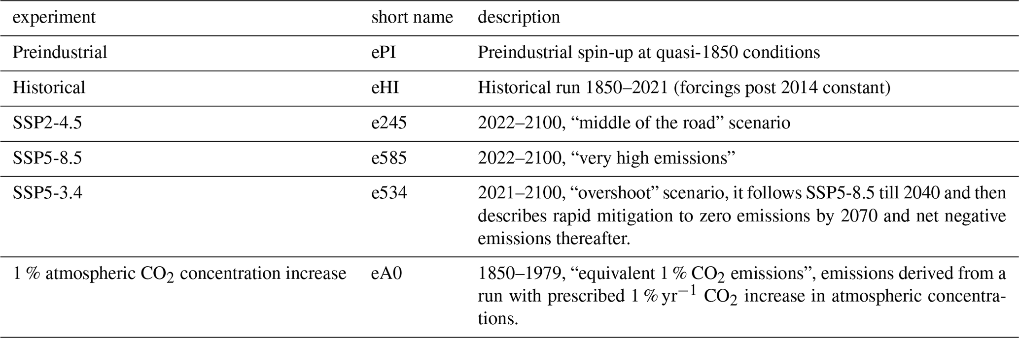
For model simulations (Table 1), we conducted a preindustrial control with 1850 conditions, a transient historical run over 1850–2021, future scenarios for SSP2-4.5, SSP5-8.5, and SSP5-3.4 for 2022–2100 and a compound 1 % increase in CO2. For the historical simulations and the SSPs we used CO2 emissions (not atmospheric concentrations) from input4mips files (Hoesly et al., 2018; Gidden et al., 2019) for the period 1850–2014 and constant thereafter, while for non-CO2 GHGs we follow CMIP6 specifications for prescribed concentrations from 1850–2014 (Meinshausen et al., 2017) and use concentrations from the NOAA Global Monitoring Laboratory from 2015 to 2021 (Lan et al., 2022b). For the eA0 (the compound 1 % run) we back-calculated implied emissions of CO2 from a concentration driven compound 1 percent run and we used those to force the eA0 scenario. All other GHGs and aerosols are prescribed following the CMIP6 specifications. The datasets used for model evaluation are shown in Table 2.
3.3 Datasets used for model assessment
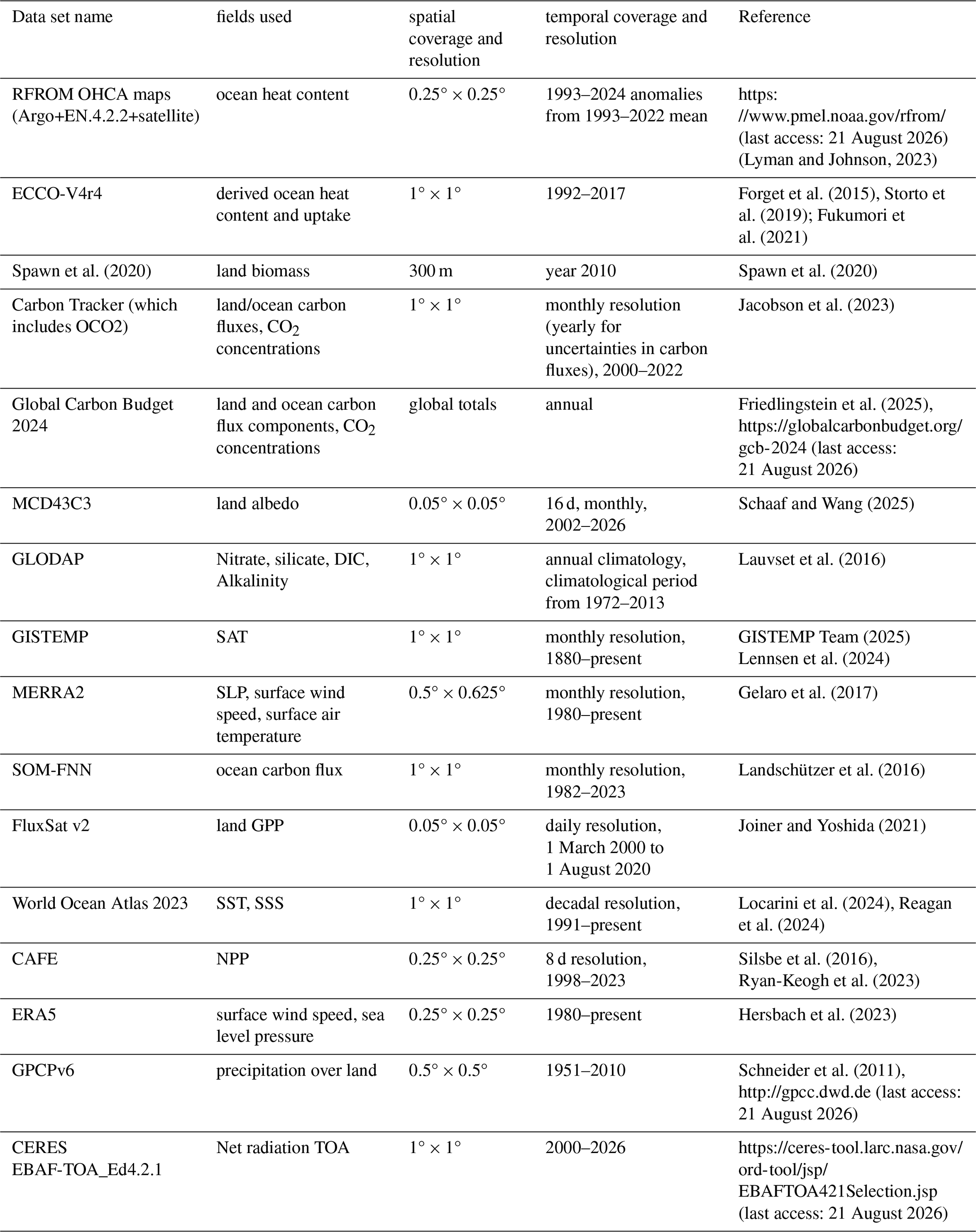
The datasets used for data evaluation are described in Table 2, where the fields used, the spatial and temporal coverage, the resolution and a key reference are also provided.
Table 2Observational and reanalysis data used for model assessments.
4.1 Preindustrial control simulation
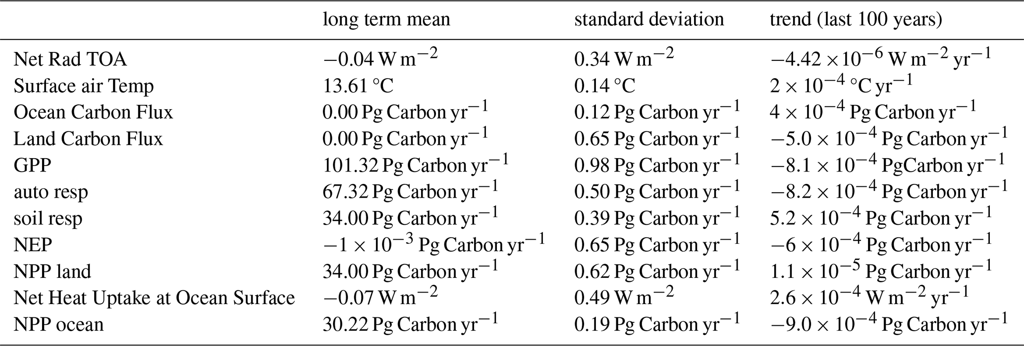
Figure 3 shows that surface exchanges and properties are in equilibrium for at least the last 500 years of the pre-industrial control simulation (under 1850 conditions) and Table 3 lists their long-term mean, standard deviation and trend. Radiative balance at the top of the atmosphere (TOA) is −0.04 ± 0.34 W m−2 (Fig. 3a and Table 3). Surface air temperature (Fig. 3b) has a small drift of about 0.02 °C per 100 years. Net land carbon flux is 0 ± 0.65 PgC (Fig. 3c), with a long-term trend of −0.05 PgC per 100 years (Table 3) while gross primary production (GPP), autotrophic and soil respiration (Fig. 3d, e, f respectively) have small trends, and so do net ecosystem production and net primary production over land (Fig. 3g and h). The largest variability arises from GPP while the largest trend from soil respiration (Table 3). Ocean carbon uptake (Fig. 3i) is at equilibrium with some slow variations of about 50-year scales and of the order of ±0.12 PgC yr−1 (Table 3). Net primary productivity in the ocean (Fig. 3j) is about 30 PgC yr−1 which is low compared to 50–60 PgC yr−1 from observations (Westberry et al., 2023). Net heat flux (Fig. 3k) is out of the ocean by 0.07 W m−2 with a large interannual variability of the order of 0.49 W m−2 (Table 3) and a small positive trend of W m−2 per 100 years. Global mean precipitation is about 2.95 mm d−1. Figure 3 also shows a comparison with the CMIP6 version of the model, denoted here as “CC” (pink lines). Due to the incomplete spinup of that version of the model, both NPP on land (including gross primary production, autotrophic and soil respiration) and in the ocean had significant trends, which imparted a 0.2 °C warmer temperatures.
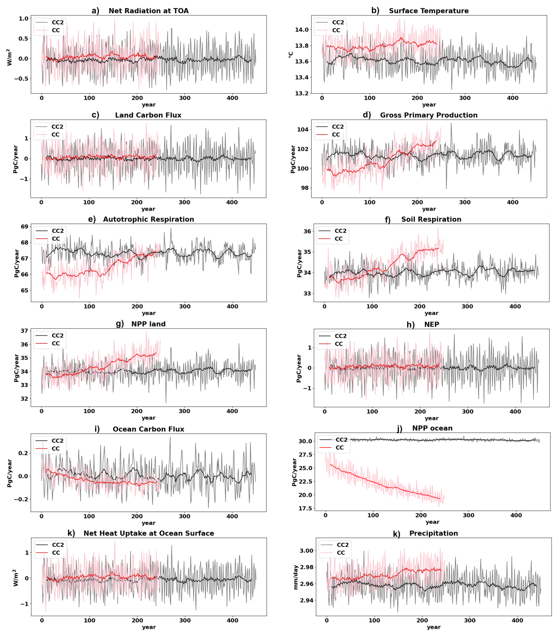
Figure 3Temporal evolution of preindustrial control fields: (a) net radiation at top of the atmosphere (TOA), (b) surface air temperature, (c) land carbon flux, (d) gross primary production (GPP), (e) autotrophic respiration, (f) soil respiration, (g) net primary production on land (NPP = GPP − autotrophic respiration) (h) net ecosystem production (NEP = NPP − soil respiration), (i) ocean air-sea carbon flux, (j) net ocean primary production (NPP ocean), (k) net heat uptake at the ocean surface, (k) precipitation. Annual mean fields for the CC2 model are shown in gray and for the previous model version (CC) are shown in pink. 20 year averages are shown in black. The horizontal axis is in years from the PI control run. Units are shown on the vertical axes. All fluxes are positive down into the surface (land or ocean).
Table 3Mean, standard deviation and trend over the last 100 years of the PI control run.
Spatial distributions of the preindustrial fields are shown in the Supplemental Material (Fig. S5). Annual mean atmospheric CO2 concentrations peak at the equator (Fig. S5a) with values around 284.5 ppm and lowest values at high latitudes about 283.7 ppm. The largest interannual variability (Fig. S5b) appears over tropical land regions and in the equatorial Atlantic and is associated with the large interannual variability due to ENSO (Kelley et al., 2020). Surface air temperature (Fig. S5c and d) shows a strong zonal variation with warmer temperatures over low latitudes and significantly colder at high latitudes, North America and Asia. The largest variability appears over the eastern tropical Pacific and in the Arctic Ocean, rim associated with natural modes of variability which are stronger than observed in our simulations (Kelley et al., 2020). The air-to-land flux is largest in the continental North America and the northern Eurasian continent (Fig. S5e). The Amazon is a weak source due to Model's warm and dry bias in this region, and the high latitudes are net sinks due slow soil carbon storage in these cold regions, while the largest variability is present in Europe and North America, tropical Africa and the Amazon regions (Fig. S5f). The ocean carbon flux has a strong sink in the North Atlantic and the Southern Ocean (Fig. S5g), particularly the Labrador Sea and the Greenland-Iceland-Norway (GIN) Seas. World ocean subtropical gyres are regions of carbon uptake whereas the tropical belt is outgassing CO2 to the atmosphere with peak values in the eastern Equatorial Pacific and secondary peaks in the Benguela and Canaries current upwelling regions. The largest variability in the ocean sink is exhibited in the North Atlantic subpolar gyre (mostly in the GIN seas and the Gulf Stream separation region) as well as in the tropical upwelling regions (Fig. S5h). The net ocean heat flux peaks in the tropical belt (Fig. S5i) where the ocean takes up heat from the atmosphere and is lowest in the North Atlantic, specifically along the Gulf Stream, the Labrador and Irminger Seas and the GIN seas, where the ocean releases heat to the atmosphere. The largest ocean heat flux variability emerges in the eastern tropical Pacific Ocean, and the North Atlantic subpolar regions (Fig. S5j).
4.2 Historical simulations
Global mean atmospheric CO2 concentrations agree with observations (Fig. 4a) with the largest discrepancies between 1900 and 1970. CC2 historical concentrations are improved compared to CC (Ito et al., 2020) due to fixing the bug with land-use change forcing files. The small underestimation of atmospheric CO2 in CC2 stems from insufficient land uptake and is consistent with the higher energy imbalance at the top of the atmosphere (Fig. 4e). Both land and ocean carbon uptake underestimated in comparison to CarbonTracker (Figs. 4d, f and S4b) over 2000–2022 but may be overestimated over the longer historical period (more discussion on land and ocean carbon sinks below) while the ocean sink is overestimated compared to SOM-FNN. Spatially positive biases up to 1.5 ppm are found over the northern hemisphere land and ocean especially the high latitudes and similar negative biases are found in the Southern Hemisphere, especially over the tropical forest regions (Fig. 5a1, a2). Generally, CC2 carbon fields as well as surface air temperature are improved compared to the CC version of the model (pink lines in Fig. 4). This is due to better spin up of the soil carbon pool and the preindustrial ocean carbon flux. The carbon disequilibrium affects substantially the cumulative heat uptake in Surface air temperature agrees well with reanalysis products in terms of trend (Fig. 4b). The model overestimates the cooling associated with Pinatubo (1991–1992) and generally shows larger interannual variability than the observations after 1950 possibly related to the strong ENSO variability (Kelley et al., 2020). Surface temperature anomalies from preindustrial track the GISTEMP observations very well (Fig. 4c) particularly after the 1950s. Between 1875 and 1950 the model is warmer than the baseline than the observations, and this is even though there is somewhat less atmospheric CO2 in the model than was observed. Spatially, the biases are more pronounced in the Arctic (by about 4 °C), the GIN Seas and the Weddell Sea (by about 2 °C), while the Eastern Pacific is warmer in the model by about 1–2 °C, the subpolar North Atlantic is colder by about 1–2°, the Southern Ocean in general is warmer by about 1 °C, and the Indian Ocean is colder by 1 °C (Fig. 5b1, b2).
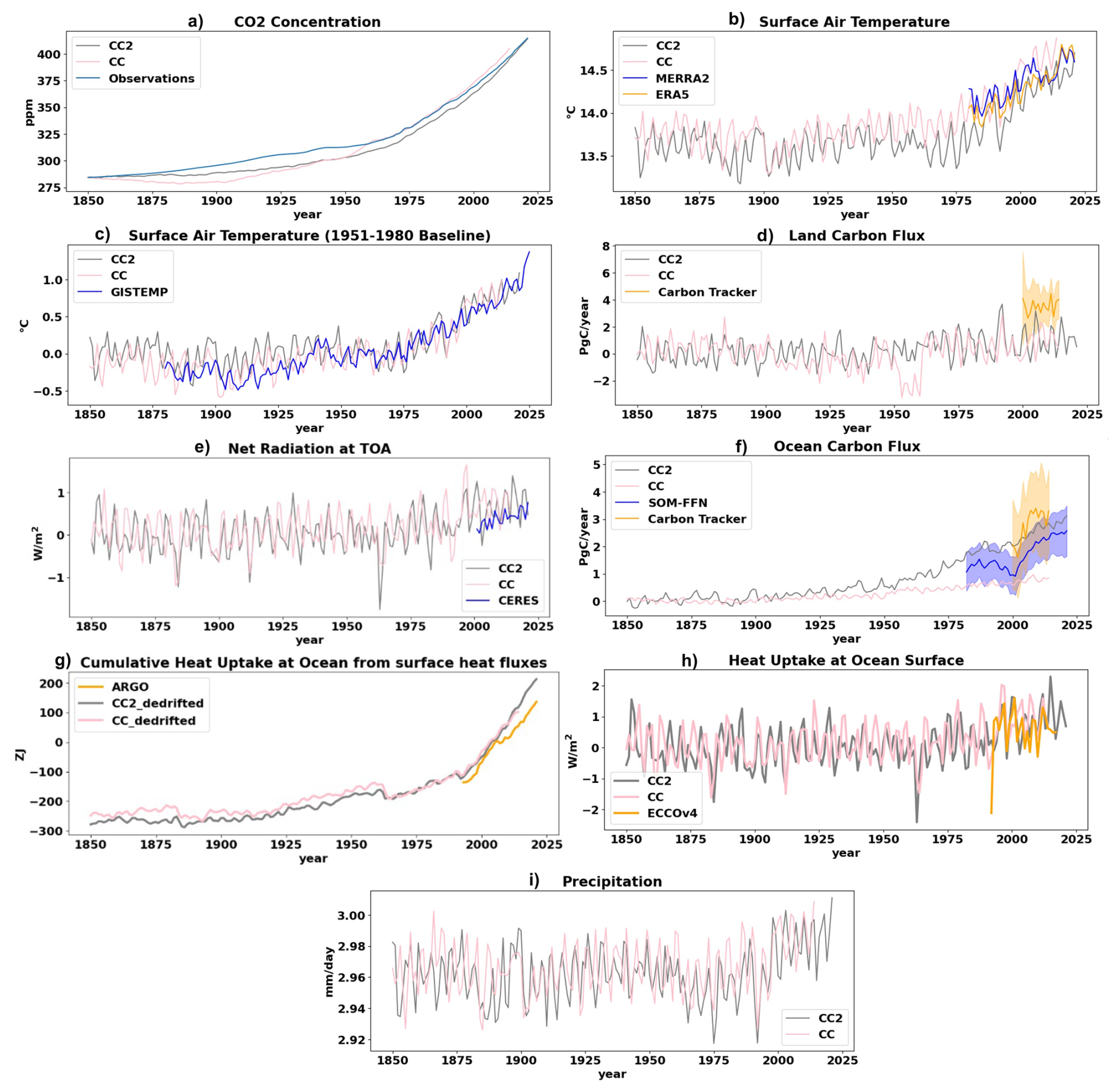
Figure 4Historical annual Time series of (a) atmospheric CO2 concentration from the model (eHI) and observations from input4mips (Meinshausen et al., 2017) from 1850 to 2015, and from the NOAA Global Monitoring Laboratory from 2015 to 2021 (Lan et al., 2022a, b), (b) surface air temperature (annual mean timeseries) and superimposed estimates from ERA5 and MERRA2 (see Table 3), (c) change in surface air temperature from the average over the period 1951–1980 and GISTEMP, (d) air-to-land carbon flux from the model (eHI) compared to observations from the Carbon Tracker (shaded is the uncertainty of the annual mean based on the averaging of inversions that consider different prior estimates of fluxes and their uncertainties; Jacobson et al., 2023), (e) net radiation at the top of the atmosphere (TOA) compared to observations from CERES 2000–2026 (f) air-sea carbon flux from the model compared to observations from SOM-FFN and Carbon Tracker (2000–2022) (shaded is the uncertainty around the annual mean, stemming from a combination of uncertainties including (i) the gridding of SOCAT observations, (ii) the RMS error between the SOM-FNN estimates and the gridded observations, and (iii) the uncertainty stemming from the chosen air-sea flux parametrization; Landschützer et al., 2016), (g) cumulative heat uptake in the model and comparison to estimates from Argo, both timeseries are anomalies from the 1993–2022 mean, the model timeseries are dedrifted using the linear PI drift, (h) ocean heat flux and comparison to estimate from ECCO-V4r4, years 1992–2017, (i) Precipitation. Black lines refer to the current model version (CC2) and pink lines to the previous model version (CC). Observations are shown in color. It should be noted here that model forcings post-2014 remain constant at 2014 levels except for atmospheric non-CO2 greenhouse gases which follow observations from NOAA-GML (Lan et al., 2022b), a fact to be considered in model-to-observation comparisons post 2014 shown in this figure.
Precipitation (Fig. 5c1, c2) in the historical eHI simulation compared to land surface precipitation observations by the Global Precipitation Climatology Centre (GPCC), National Oceanic and Atmospheric Administration (NOAA), Full Data Reanalysis Version 6.0, over 2001–2010, shows that the model has an extensive dry bias over the tropics, a persistent model bias also documented in Kelley et al. (2020) for the ModelE-2.1 contribution to CMIP6. This bias is particularly pronounced in the Amazon Basin, which is a persistent issue in GCMs in general (Respati et al., 2024). The ModelE dry bias is also strong in India and Indonesia. The model has a wet bias in Western China and the West Coast of South America along the Andes.
Average sea level pressure (Fig. S6a, b) is higher than observations by more than 10 mb over Greenland and Antarctica and the mountainous ranges in south-east Asia and South America. It is systematically underestimated over the ocean by about 5–10 mb. Surface winds are weaker than in observations (Fig. S6c, d) by more than 5 m s−1 over Greenland and Antarctica, 3–5 m s−1 over the mid- and southwest US and Patagonia, Europe and Northern Africa, and by 2–4 m s−1 over ocean subpolar gyres, an issue with all previous modelE versions, and which led to the inclusion of the “gustiness” term (see Sect. 2.7).
Global mean air-to-land carbon (net biome productivity, NBP) flux (Fig. 5d) hovers at a net flux of zero in the 20-year moving average over 1850–1942, after which the trend becomes a net sink. Over 2000–2022, it is underestimated compared to Carbon Tracker as it lies below the mean and outside the envelope of interannual variability in this dataset. Interannual variability is also much higher amplitude in the model, due sensitivity of the land carbon to ModelE's higher amplitude interannual surface temperature variability from simulated El Niños. A more detailed breakdown of eHI time series of the land fluxes (GPP, autotrophic respiration, soil respiration, emissions due to land use change, NPP, NBP, NEP) and soil carbon stocks are provided in Fig. S7, which shows both the annual totals and their 20-year running means to show trends. These show all natural fluxes accelerating after ∼ 1960. Regionally, the underestimation (which exceeds 20 mol CO2 m−2 yr−1) stems from weaker Amazon and African rainforest uptake as well as weaker boreal forest uptake (Fig. 5d). The cumulative land carbon sink 1850–2023 estimated by the Global Carbon Budget 2024 is 220 ± 60 PgC (Friedlingstein et al., 2025), whereas in the historical simulation the model reaches a cumulative sink of only 56.6 PgC by 2021 (Fig. S7b). CarbonTracker and other flux inversion models estimate generally lower NBP than DGVMs, which Bastos et al. (2020) attribute to disagreement on NBP interannual variability responses to El Niño and uncertainties in land use emissions, particularly in South America and Southeast Asia. Meanwhile, based on remote sensing observations of vegetation change, Randerson et al. (2025) find that forest growth is far less than predicted by the ensemble of DGVMs in the GCB2023; the remote sensing data yield an estimated net land carbon sink over 2000–2019 of 0.8 ± 0.7 PgC yr−1, whereas the GCB2024 DGVMs estimate a high 1.32 ± 0.2 PgC yr−1 due to unrealistic predictions of forest greening or densification. Our model estimates 1.12 ± 1.04 PgC yr−1 over this period. The GCB2024 DGVM estimates of earlier preindustrial through 20th century deforestation emissions also rely on highly uncertain predictions of forest biomass and land use change. Observational constraints of vegetation biomass remain a challenge: inventory and satellite surface observations of global total vegetation biomass estimates still range over a wide 380–536 PgC (Erb et al., 2018), while more recent radar and lidar satellite data products of forest heights are still being processed to produce new global biomass estimates, which we detail more later.
In Fig. 5e, the emissions from land cover and land use change (LCLUC) are plotted together with the estimates of the Global Carbon Budget 2024 (GCB 2024) (Friedlingstein et al., 2025), which span 1960–2024 only. These show that our land cover change (LCC) emissions strongly underestimate the mean estimate of the GCB2024 by more than 1 PgC yr−1, and is outside their low (less negative) estimate; the model underestimate is very likely because our model does not include deforestation/forest regrowth, wood harvest, or peat emissions, but only land cover conversion from natural vegetation to croplands. Therefore, our model's LCC emissions from the preindustrial period to 1960 likely also underestimate total LCLUC emissions by a similar magnitude, leading to our underestimate of atmospheric CO2 (Fig. 4a).
Based on our model physics, we would expect the simulated underprediction of atmospheric CO2 to be explained by the ModelE land model's lack of full representation of certain components of land use change (LUC). Figure 4e shows the eHI net carbon emissions due to LUC compared to the breakdown of components of LUC change emissions estimated by the Global Carbon Budget 2024 (GCB2024, Friedlingstein et al., 2025). Although the model represents deforestation that converts forest to croplands or other cover types, it does not represent wood harvest or deforestation that results in degraded forest; also, the model is not a fire-enabled model, so fire emissions associated with deforestation and peatlands are not represented. Therefore, the eHI emissions miss on average 1.0 ± 0.3 PgC yr−1 over 1959–2021 compared to GCB2024 mean net LUC emissions. Since deforestation emissions were higher over the earlier historical period and the model misses these emissions, we would expect the underpredicted net emissions to the atmosphere to result in the model's slightly lower atmospheric CO2 concentrations, which catch up to the observed as deforestation declined in recent decades. Given the much lower NBP estimated by Randerson et al. (2025), the high bias of GCB2024, and uncertainties in flux inversion models, despite the eHI simulation's comparatively low cumulative land carbon sink, it may be that ModelE's land carbon sink is overpredicted in the context of the model's simulated flux components (Fig. S7), explaining our low predicted atmospheric CO2. These discrepancies highlight the continued large uncertainties in land carbon stocks and fluxes.
Model SST (averaged over 1991–2020) is colder than World Ocean observations by about 2–4 °C in the subArctic regions (Fig. 5f1, f2). The tropical eastern Pacific Ocean and Tropical Atlantic are warmer than observations by about 2–4 °C, whereas the Southern Ocean is warmer than observations by about 2–4 °C. The North Atlantic Current region and the Arctic are colder by about 2–5 °C. The model historical climatology 1991–2020 of the sea surface salinity (SSS, Fig. S6f) is fresher than observations (Fig. S6e) by about 4 psu in the Eurasian side of the Arctic Ocean, and about 2 psu in the tropical regions of the central Pacific Ocean, the Atlantic Ocean and the Indian Ocean. The model overestimates salinity by about 2 psu in the tropical eastern Pacific Ocean and in the Arabian Sea and the Bay of Bengal in the Indian Ocean. The SSS biases largely reflect biases in evaporation and precipitation patterns over the global ocean (Kelley et al., 2020; Miller et al., 2021) which are in turn related to biases in surface pressure and surface winds (Fig. S6a, b, c, d).
The ocean carbon flux (Fig. 5f) lies between the observation-based estimates SOM-FFN and Carbon Tracker and within both datasets' interannual variability. Spatially, ocean carbon uptake negative biases (up to 5 mol CO2 m−2 yr−1) are associated with strong wind-driven circulation and fronts (e.g. over the Gulf Stream, the Equatorial trade winds and the Southern Ocean subtropical front (Fig. 5g1, g2) whereas positive biases (up to 6 mol CO2 m−2 yr−1) are linked to convection sites in the North Atlantic (Labrador Sea, Irminger Sea and GIN Seas) and the Antarctic Circumpolar Current (ACC) region. Subtropical gyres and the tropical Atlantic and Indian Oceans also show positive biases. Tropical ocean outgassing is also stronger in the GISS model, despite the weaker than observed winds and warmer SSTs there, because the pco2 disequilibrium is larger than observed, due to a combination of low productivity (as we describe below) and also because the vertical sinking of organic carbon below the thermocline is too small, which is discussed in more detail in Lerner et al. (2024).
Net primary productivity is underestimated everywhere in the world's oceans compared to CAFE observations by about 100–200 mgC m−2 d−1 (Fig. 5h1, h2), except in the subtropical gyre in the North Atlantic and in the Benguela and Canaries current regions. The generally low bias in NPP results from at least two issues. First, there was an error in our ocean radiative transfer routines that compute the direct and diffuse radiation that enters and leaves each ocean layer. For each layer, we incorrectly used the layer depth (distance from the ocean surface to the layer), rather than the layer thickness (distance between upper- and lower-layer boundaries), when computing the amount by which direct radiation should be reduced from the top to the bottom of each layer. This resulted in too little shortwave radiation reaching subsurface waters, reducing NPP. Second, phytoplankton in our model currently do not acclimate in ambient light levels, so that chl:C ratios in the sun-lit surface are the same as those deeper in the water column. Acclimation is expected to increase the growth of phytoplankton and NPP under low-light conditions (Geider et al., 1998), so the absence of this process in our model likely also contributes to lower productivity levels. We also should note that our comparison only encompasses a single NPP product, that derived from the CAFE algorithm applied to the Ocean Colour Climate Change Initiative merged remote sensing data product (Ryan-Keogh et al., 2023). NPP products are known to vary widely depending on the algorithm applied, particularly in the Southern Ocean but also to a significant extent in the Northern high latitudes. For example, using the same dataset, the Eppley-VGPM algorithm yields roughly the productivity of the CAFE algorithm in the Southern Ocean (Ryan-Keogh et al., 2023). Therefore, despite improvements that need to be incorporated, how well our model performs in some ocean environments, particularly the Southern Ocean, remains unclear. Finally, we note that a few regions, in particular the Benguela and Mauritanian upwelling regions, display positive NPP biases. The cause of these biases remains a subject of future investigation, although a potential contributing factor is the fact that our model lacks water column (Lam and Kyupers, 2011) and benthic denitrification (Dale et al., 2014), which could result in too much upwelling of nitrate in these regions.
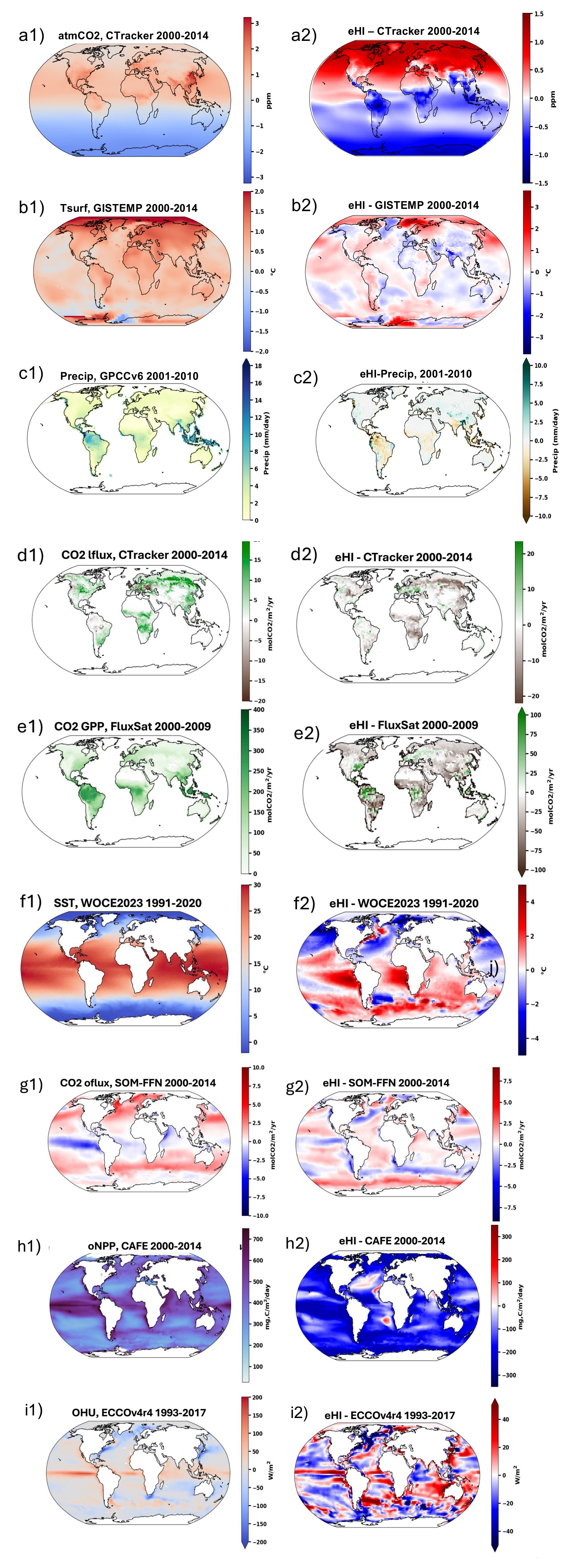
Figure 5Observational and observation-based estimates and model spatial biases averaged over the period of the observations. (a1) Atmospheric CO2 concentration anomalies from the global mean from Carbon Tracker averaged over 2000–2014. (a2) Atmospheric CO2 concentration anomalies, model biases from Carbon Tracker, (b1) GISTEMP average 2000–2014, (b2) Surface air temperature model biases from GISTEMP v4 (anomalies from 1951–1980) averaged over 2000–2014, (c1) Precipitation average 2001–2010 from GPCPv4, (c2) historical precipitation biases over land fro GPCPv4, (d1) Land carbon flux taken from Carbon Tracker between 2000–2014, (d2) land carbon flux model biases in the model compared to Carbon Tracker, (e1) land GPP taken from FluxSat between 2000–2009, (e2) GPP model biases in the model compared to FluxSat, (f1) Sea surface temperature (SST) averaged from the period of 1991–2020 from World Ocean Atlas 2023 (WOA2023), (f2) historical SST biases in the model compared to WOA2023, (g1) ocean carbon flux observations from SOM-FFN averaged over the period 2000–2014, (g2) Ocean carbon flux biases in the model compared to SOM-FFN, (h1) Ocean net primary productivity (NPP) averaged from 2000–2014 from CAFE (Silsbe et al., 2016), (h2) ocean NPP biases in the model compared to CAFE, (i1) ocean heat content from ECCO-V4r4, averaged over the period of 1993–2017, (i2) Ocean heat uptake bias in the model compared to ECCO-V4r4.
Ocean heat uptake anomaly from a late-20th century baseline is well in agreement with estimates from Argo floats (cumulative; Fig. 4g) and with ECCO-V4r4 (non-cumulative anomaly from preindustrial; Fig. 4h) as well as variability in the latter dataset. Spatially, the patterns of average differences between the GISS model and ECCO-V4r4 for the period 1993–2017 are within ±50 W m−2, with positive differences (GISS minus ECCO-V4r4) dominating the low latitudes and negative differences the high latitudes and the eastern Pacific Ocean (Fig. 5i1, i2). More specifically, ocean heat uptake averaged over 1993–2017 is underestimated in the model by more than 40 W m−2 in the North Atlantic subpolar gyre and the ACC region (Fig. 5i1, i2) due to the lower wind speeds there, whereas it is overestimated over other regions with strong currents (e.g. the eastern Pacific and eastern Atlantic equatorial current regions, the Brazilian and Benguela current regions, the Agulhas retroflection region, the eastern part of the western Australian current region, and the Kuroshio region) because the sea surface temperatures are much higher (Fig. 5f1, f2).
The changes from CC to CC2 are synopsized in Fig. S8: atmospheric CO2 increases (decreases) in CC2 by about 4 ppm in the Northern (Southern) Hemisphere. The largest changes in land carbon fluxes are an increase in Russia by ∼ 10 mol CO2 m−2 yr−1, and declines in northwestern Europe and Southeast Africa by ∼ 5 mol CO2 m−2 yr−1 (Fig. S8b). GPP is generally larger in CC2 than CC, showing increase of up to 40 mol CO2 m−2 yr−1 in central Africa and South America, though there are some regions such as the Amazon rainforest that show small declines (< 5 mol CO2 m−2 yr−1) instead (Fig. S8c). The ocean flux shows moderate increases in the subtropical regions and Southern Ocean (3–5 mol CO2 m−2 yr−1), and a large decline in the equatorial Pacific ( mol CO2 m−2 yr−1; Fig. S8d). Finally, NPP shows a large increase and decline of ∼ 200 mgC m−2 d−1 in the subtropical regions and Southern Ocean, respectively, as well as smaller decline in the subpolar North Pacific and Atlantic (∼ 50 mgC m−2 d−1; Fig. 9e)
Seasonality
The seasonal cycle of the air‐to‐sea flux of CO2 and the partial pressure of CO2 in the sea water have been extensively evaluated against several observational data sets (Lerner et al., 2021).
For the land carbon, seasonal GPP fluxes are shown in Fig. S9, compared to estimates by FluxSat v2 (Joiner and Yoshida 2021). ModelE-CC estimates annual GPP as 118.6 ± 1.5 PgC yr−1 over 2000–2009, and 124.7 ± 2.0 PgC yr−1 over 2014–2021, which is currently at the lower end of both multi-model and observation-based estimates ranging 110–170 PgC yr−1 (Anav et al., 2015; Cheng et al., 2017; Xu and Chen, 2024). The latest Global Carbon Budget 2024 cites a mean annual GPP of 130 PgC over 2014–2023 (Friedlingstein et al., 2025).
The land seasonal regional GPP patterns qualitatively agree with FluxSat estimates (Fig S3). However, there are stark regional differences. ModelE-CC simulates much higher GPP in the Amazon and Congo Basins in all seasons compared to FluxSat. Since ModelE has a warm/dry bias in these regions, we would expect GPP to be low. The FluxSat data are expected to be a lower bound estimate when based on flux tower data and not utilizing solar-induced fluorescence (SIF) data. Therefore, the higher ModelE GPP may be appropriate. In arid and semi-arid regions outside the Amazon and Congo in South America and Africa, ModelE predicted GPP is much lower than FluxSat; these mostly mixed shrubland and grassland areas are strongly controlled by soil moisture availability, and ModelE has a dry bias in these areas, leading to lower GPP. The shrubland PFT is also one for which the Ent TBM lacked a Fluxnet site to evaluate simulated fluxes, so parameterizations of leaf photosynthetic capacity and respiration may be improved. In the northern high latitudes, the season MAM exhibits delayed spring greenup and the summer has low productivity due to ModelE's extended cold bias, while mid-latitude croplands in the Eastern U.S. and Europe are predicted to have much higher GPP than FluxSat estimates. The Northern Hemisphere differences between ModelE and FluxSat decline in the fall, SON, when deciduous trees senesce.
4.3 Heat and Carbon storage on land and in the ocean
Long term storage of heat and carbon in the ocean and on land is important for the control they exert on future climate change.
4.3.1 Ocean storage
A comparison of heat storage trends at different levels in the ocean in the GISS model and the ECCO-V4r4 ocean state estimate (Fig. 6) shows that, in general, the GISS ocean model stores more heat in the subtropical gyres in the North Atlantic as well as the Atlantic sector of the Antarctic convergence zone at all levels. ECCO-V4r4 stores more heat in the subpolar North Atlantic and in the deep Southern Ocean around Antarctica. The deep western boundary current which is clearly outlined in the GISS ocean model at depths below 600 m is not as clearly identified in ECCO-V4r4. The GISS model also stores more heat in the upper North Pacific Ocean compared to ECCO-V4r4, however the latter stores more heat in the tropical Pacific. Differences in the storage regions and depths will influence the response of the ocean model to future forcing changes, as heat stored closer to the surface and at higher latitudes will more easily be released to the atmosphere compared to heat stored at lower latitudes.
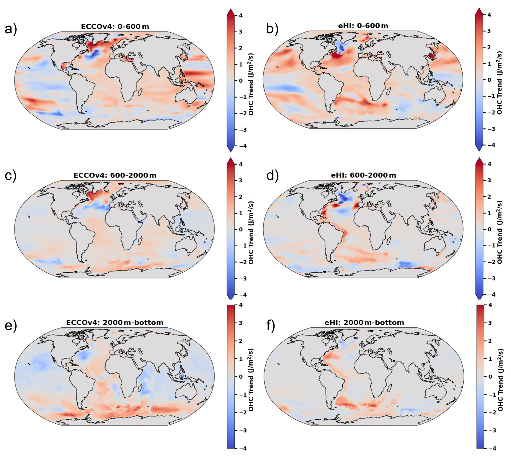
Figure 6Ocean heat content trend (J m−2 s−1) for the period 1993–2017 in ECCO-V4r4 and GISSE2.1-CC2, vertically integrated: (a, b) from surface to 600 m, (c, d) 600–2000 m, (e, f) 2000 m-bottom.
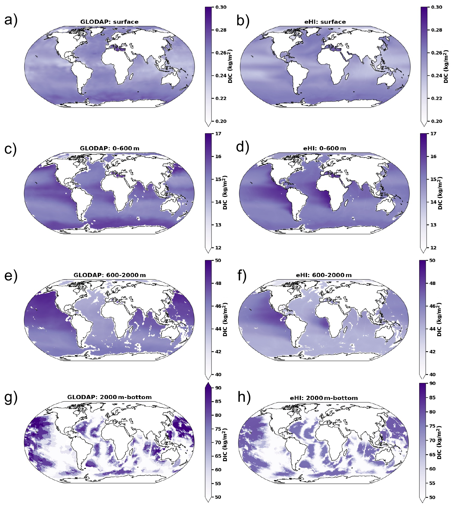
Figure 7Integrated DIC (kg m−2) from GLODAP and GISS eHI for the period 1993–2014 at different levels: (a) surface, and integrated over (b) 0–600 m, (c) 600–2000 m, (d) 2000 m – bottom.
Compared to GLODAP (Fig. 7), the model overestimates carbon stored in the upper ocean (0–600 m) of the tropical/subtropical regions, especially in the Atlantic (Fig. 7c, d). The model also underestimates the storage of carbon in intermediate waters (600–2000 m), particularly in the North Pacific (Fig. 7e, f). These findings are consistent with those of Lerner et al. (2024) that the flux of carbon beneath 100 m is too high and the transfer efficiency (ratio of carbon export at depth to carbon export at 100 m) is too small, although that study was limited to the equatorial Pacific. High export fluxes near the surface may be due to overgrazing by zooplankton, as zooplankton loss terms (via linear and quadratic mortality: Eq. A32) produce the bulk of the detrital organic carbon in the model. On the other hand, the lack of remineralized DIC in deeper waters below 600 m may be due to the absence of processes that could contribute to higher detrital sinking speeds, such as a lack of ballasting by inorganic material (carbonates and lithogenics; Armstrong et al., 2001), and our use of a single-particle class model rather than multiple size classes that would encompass a wide range of sinking speeds as found in the real ocean (Burd, 2015).
4.3.2 Land carbon storage Plant labile carbon and soil carbon distribution
With canopy structure and seasonal LAI otherwise prescribed in Ent, there are two prognostic carbon pools: labile carbon (also known as non-structural carbohydrate, NSC) and soil carbon. The labile carbon pool is the net of carbon uptake from photosynthesis plus retranslocation from senescing foliage minus autotrophic respiration. In the Ent TBM, autotrophic respiration for most PFTs is tuned to Fluxnet sites to achieve carbon balances with well-quantified site canopy structure (Kim et al., 2015). The global prescribed canopy structure in the simulations in this study may not be in climatological equilibrium with the simulated climate for several reasons. The LAI is from observations from the specific years 2004 for LAI and 2005 for canopy heights. These satellite observations have errors or simplifications, where the spikes in MODIS LAI are largely smoothed but the interpolated monthly LAI updates in ModelE will miss the shorter time scale of green-up and senescence. The forest canopy heights derived from ICESat/GLAS used in these runs are now known to be ∼ 6 m too tall, given the recent more accurate observations of the Global Ecosystem Dynamic Investigation (GEDI) mission (Dubayah et al., 2020); this results in excess stem biomass from tall trees in the prescribed canopy structure, resulting in 533 PgC in aboveground biomass (AGB) in the eHI experiment (Fig. 8a). This is nearly twice that estimated from harmonized inventory and satellite cover data by Spawn et al. (2020; Fig. 23b, e), which is 287 PgC AGB and total 409 PgC including belowground biomass for the year 2010, or from the GEDI lidar data (Fig. 8c, f; Dubayah et al., 2022), which is 283 PgC AGB and limited to south of 53° N. The GEDI data product predicts lower tropical biomass than Spawn et al. (2020) and higher in the low- to mid-latitudes. Liu et al. (2025) estimate global AGB to be 378 PgC from satellite radar. Figure 8e, f difference maps show that the tall bias of Ent TBM forests in the Amazon and Congo Basins and in the boreal zone results in high AGB compared to the Spawn et al. (2020) and GEDI estimates. Grassland areas in eHI (Great Plains, United States; Sahel, Africa) have higher AGB than the observational estimates due to a bug in labile carbon storage for grasses in Ent. Besides only recently available satellite data on vertical canopy structure at appropriate spatial scales for vegetation heterogeneity, plant allometry parameterization remains a large issue for all DGVMs for estimating biomass (Grant et al., 2025; Liu et al., 2025; Jucker et al., 2022; Massoud et al., 2019), resulting in large uncertainties in autotrophic respiration that is a function of the plant biomass. Finally, the GCM simulated climate has regional biases; in ModelE2, the tropics have strong warm/dry bias, and in the high latitudes, a strong cold bias causes prolonged frozen soil, hence prolonged simulated winter-spring water stress and low carbon uptake. In the interest of maintaining canopy structure as close to observations as possible rather than predicting wrong vegetation cover and mortality with climate biases, we opt for managing imbalances in the labile carbon pool, instead.
The map in Fig. 8a of plant labile carbon identifies regions where there is insufficient carbon uptake in both boreal evergreen needleleaf and tropical evergreen broadleaf forests. The carbon deficit in forests in these regions is due both to simulated climate biases and overestimated forest stem biomass. The boreal zone is 8–10 °C too cold in ModelE, with frozen soils persisting from the winter into what should be the greenup period, causing water stress and reduced GPP; the Amazon Basin has a warm/dry bias causing water stress where there should not be and also reducing GPP. Excess stem biomass from the overestimation of height from the ICESat/GLAS estimate results in high mass-based autotrophic respiration. Thus, the underpredicted GPP and overestimated autotrophic respiration in these forest types results in plant carbon deficits and labile carbon near zero. The label carbon map also highlights an error in parameterization of grasses that results in too high labile carbon by a few kg m−2, particularly in the U.S. interior as was noted also for Fig. 8e, f.
In Fig. 8b, soil carbon distributions reflect high storage in the high latitudes where permafrost tends to be (ModelE does not explicitly simulate permafrost). The total soil carbon averaged over years 2002–2020 of eHIis 1693 PgC, which is virtually the same as the 1700 PgC from inventory estimates compiled by Canadell et al. (2021) and cited by the GCB2024.
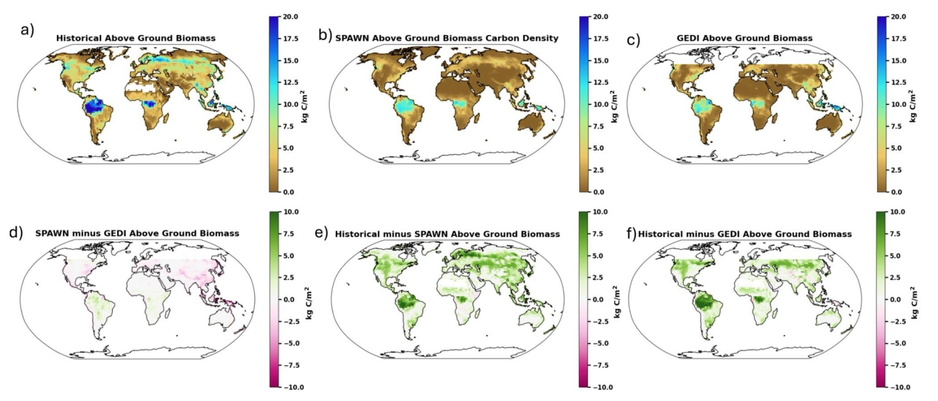
Figure 8Land carbon stocks. Aboveground plant biomass (AGB) from (a) the historical simulation (eHI), (b) harmonized inventory and satellite-based estimate by Spawn et al. (2020) (year 2010), (c) satellite observations from GEDI (25 March–22 May 2019), (d) difference between Spawn and GEDI, (e) the historical simulation eHI (year 2010) – Spawn dataset, (f) the historical simulation eHI – Spawn dataset (year 2010). Globally integrated AGB is 533 PgC for eHI, whereas it is 287 PgC for SPAWN and 283 PgC for GEDI.
4.4 Köppen-Geiger Climate Classifications
In Fig. 9, we show the Köppen-Geiger classifications of observed 2001–2009 (ERA5) climate and the simulated climates, following the classification algorithms of Kottek et al. (2006), which produce 31 climate classes, listed in Appendix Table B1. For the tropics, we implemented a slight modification. Where Kottek et al. (2006) defined a 6-month summer, we used 4-month seasons for tropical climates As and Aw (northern hemisphere, summer = June–September, winter = November–February). This modification identifies the rain shadow areas in East Africa, Sri Lanka, and maybe a little too much of northeastern Brazil.
The observed climatology was classified at 0.5° × 0.5°, because the coarser ModelE grid cannot capture a less common climate type, Dsd. We note also that because the Köppen-Geiger scheme uses only precipitation and temperature data, it cannot capture wetland areas like those in the southern end of the Amazon Basin, which are fed by stream- and riverflow; these areas classified as Aw (pink, equatorial savannah) are in reality Af or Am (dark red, equatorial rainforest, or bright red, equatorial monsoon). Compared to observations, the PI and historical runs show that ModelE2 has a warm/dry bias in the Amazon and Congo basins, producing the climates more suited to savannah than tropical forest. ModelE2 also has a cold bias in the northern high latitudes; where observed climate shows Dfb and Dfc (snow fully humid), ModelE2 simulates EF and ET (polar frost and polar tundra). ModelE simulates the Western U.S. as moister (Cs, warm temperature with dry summer) than observed (Bw and Bw, arid) and does not produce the northeast Asia Dwc climate (subarctic/boreal taiga/boreal forest). ModelE simulates Central and Western Australia as BSh (arid steppe hot), more conducive to shrubs and grasses than observed BWh (arid desert hot).
The simulated climate change between the PI and the end of the historical period shows a slight migration of high latitude climate type Dfc (bright purple, boreal forest) northward, with no changes in the mid-latitudes and tropics. This northward migration continues with the SSP future scenarios, along with encroachment of lower elevation classes to higher elevation around the Tibetan Plateau, and moistening of southern Chile.
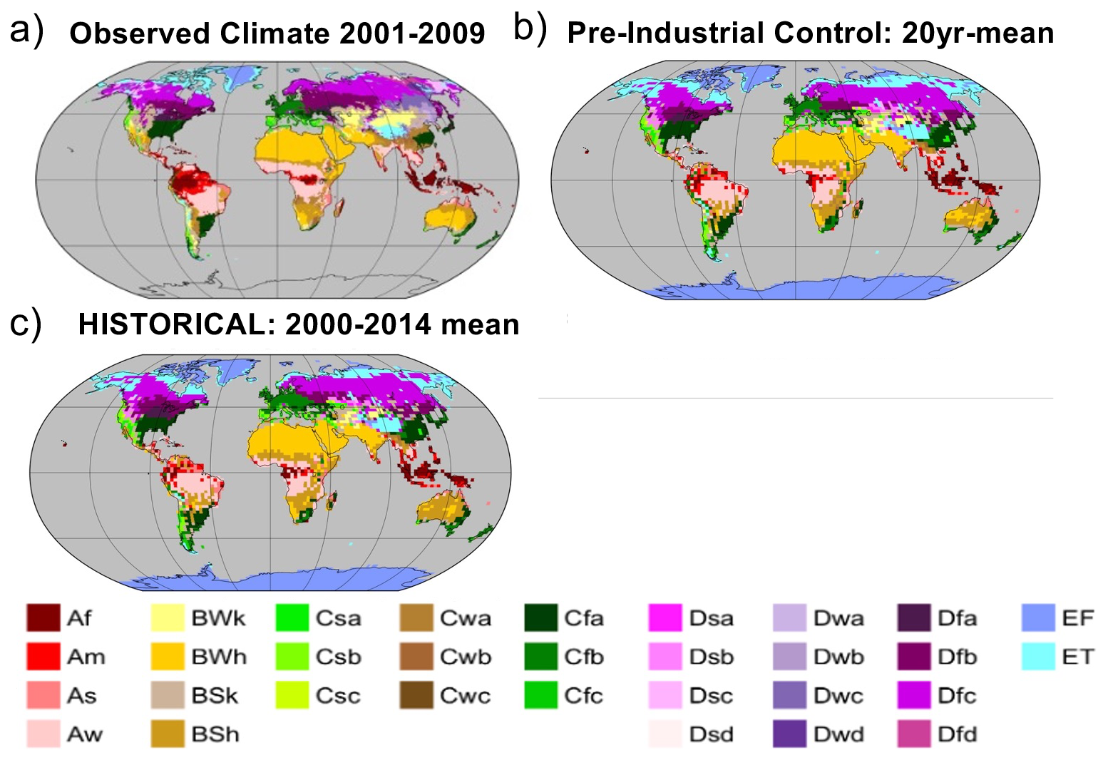
Figure 9Köppen-Geiger climate classifications of (a) observed 2001–2009 climatology (ERA5), (b) the pre-industrial and (c) historical runs. Colorscheme is from Kottek et al. (2006). Observed climate from ERA5 at 0.5° × 0.5° resolution.
In this paper we described the development, skill and characteristics of the NASA GISS Earth system model coupled to emissions of CO2. With respect to the CMIP6 version of the emissions driven model (CC: Ito et al., 2020), GISSE2.1-CC2 has the same physical climate formulation with non-interactive aerosols which are prescribed from fully interactive runs. Additionally, GISSE2.1-CC2 includes interactive oxygen and improved iron distributions.
The main advantage of CC2 vs CC is that the CC2 model has been run to equilibrium more consistently than in CC (CMIP6). The land carbon physics are the same as in CMIP6, but the improved LUHv2 historical crop cover dataset has been used to replace older estimates used in CMIP6.
The model has improved pre-industrial carbon fields and lower carbon drift than the previous version of the model (Ito et al., 2020). It also includes a better crops and land use forcing product (GCB-LUH2 2020) and various improvements in the ocean carbon cycle (iron ligands, oxygen coupled to ocean biogeochemistry, improved nitrogen fixation). However, ocean primary production remains as low as in the CMIP6 version of the model. While some of the model biases (Latto and Romanou, 2018; Marshall et al., 2017; Romanou et al., 2017) are certainly attributed to biases in the underlying ocean model (e.g. low wind speed, Arctic circulation and hydrography) many of the biases in the carbon cycle stem from biases in different parameterizations (e.g. remineralization and nitrogen fixation), missing denitrification sinks for nitrate, sea ice effects on primary production, and a discrepancy between the iron distributions in the preindustrial control climate and the historical simulations which leads to a strong decline in productivity early in the 20th century simulation (Lerner et al., 2021).
The land carbon model overall predicts global land GPP, NPP, and soil carbon well within the mean of estimates from multi-model intercomparisons (Friedlingstein et al., 2025) of fluxes, and nearly exactly matches inventory compilations for soil carbon (Canadell et al., 2021). Predicted GPP (and NPP) is at the lower end compared to other current DGVMs. The model's global GPP is found to be 127 Pg yr−1 in 2021 while uncertainties estimated by Cheng et al., 2017 (the primary source for IPCC Sixth Assessment Report Working Group, Canadell et al., 2021, and the GCB2024) and 146.1 ± 21.3 Pg yr−1. The model grossly overpredicts vegetation biomass due to prescription of forest heights from early satellite lidar estimates from ICESat/GLAS (Simard et al., 2011), which we plan to replace with new more accurate estimates from GEDI and ICESat-2. There is a bug in the storage of plant labile carbon for grasses, causing excess accumulation in the plants instead of senescing as litterfall. Meanwhile, the model's configuration in biophysics-only mode with only prescribed vegetation structure does not allow for vegetation change through greening, mortality, or competition; however, the prognostic carbon pools of plant labile carbon and soil carbon provide useful diagnostics for vegetation responses to climate changes and CO2 fertilization, and the assumption of mature forest canopy structure may be closer to reality than the overpredicted forest growth currently from DGVMs in the GCB2024. The model does not represent several LUC processes, notably deforestation, wood harvest, vegetation and peat fires, resulting in missing about 1 PgC yr−1 in LUC-related emissions compared to GCB2024 models over 2009–2019, and that deficit is likely larger over the preindustrial through 20th century. The cumulative land sink since 1850 is still very poorly constrained, so it is better not to reference other estimates currently, which differ wildly, but rather to scrutinize self-consistency within the model. We conclude that the model's lack of these LUC processes causes a deficit in simulated cumulative fluxes to the atmosphere, relative to the model's other flux components, and may explain ModelE's slightly underpredicted atmospheric CO2 over most of the historical period.
Overall, the ModelE2.1-CC2 predicts the atmospheric concentrations of CO2 consistent with prescribed emissions given by Community Emissions Data System (CEDS) and much the mean inter-model difference of 7 ppm found in Hajima et al. (2025).
The current version (NASA ModelE2.1-CC2) has been included in several model intercomparison studies where its performance can be directly assessed against other state-of-the-art Earth system models. In coordinated experiments with a data-assimilated model of the historical ocean, the Ocean Circulation Inverse Model (OCIM; Holzer et al., 2021; DeVries, 2014) historical and future emissions of CO2 were estimated from trawling disturbances to the ocean floor (Atwood et al., 2024). From the GISS model both concentration driven as well as emissions driven simulations were used and the results showed that the GISS model (ModelE2.1-CC2) estimates of the fraction of CO2 that escapes to the atmosphere agree very well with OCIM and OCIM for both concentration and emissions driven runs, with the latter providing significant uncertainty associated with internal climate variability of CO2 which is not included in concentration driven simulations.
In a 13-model intercomparison study and an ambitious effort to estimate properly the remaining carbon budgets (Silvy et al., 2024) till 1.5 and 2° warming levels, was shown to be consistently within the model spread, except perhaps the land carbon sink, which is however very poorly constrained by observations.
Similarly, in Sanderson et al. (2025) which investigated 10 comprehensive climate models' and 3 intermediate complexity models' response to positive, zero and negative emissions of CO2, the GISS ModelE2.1-CC2 response was within the uncertainty range of the ensemble mean and only exhibited the strongest response in the later phase of the carbon dioxide removal experiments due to the weakened AMOC.
Future development in the ocean biogeochemistry will focus on adding diel migration as an improvement to the biological pump parameterization in the model, coupling ocean biogeochemistry with sea ice, the addition of denitrification and closing the nitrogen cycle, adding particulate inorganic carbon to improve alkalinity and the CaCO3 pump, improvements in the underwater light distributions and photoadaptation of phytoplankton, and coupling to physical ocean via albedo and changes in stratification.
Future developments for the land model include releasing a geometric optical radiative transfer (GORT) canopy model for global production runs. This canopy radiative transfer model, the Analytical Clumped Two-Stream (ACTS) model (Ni-Meister et al., 2010; Yang et al., 2010) leverages the cohort structure of the Ent TBM analytically to solve for foliage clumping in heterogeneous canopies in two-stream scheme. This approach simulates vertical foliage profiles (VFP) as observed by satellite lidar, which will enable ingestion of these profiles from GEDI and ICESat-2. The combination of foliage clumping prediction and VFPs then allows prediction of the effects of zenith angle and gaps on canopy spectral albedo, vertical light profiles for light competition, and transmittance of radiation to the ground for predicting soil temperature and snowmelt. We have also completed an analysis (Grant et al., 2025) of the Tallo dataset of tree allometry (Jucker et al., 2022), in which we identified significant distinctions between plant functional types; these new allometric parameterizations will be introduced into the Ent TBM along with more recent satellite lidar observations of forest canopy heights. Combining these canopy physics and updated canopy structure and allometry will allow reduction in uncertainty in vegetation biomass; it will provide a fusion between vegetation demography for simulating plant competition for light with emerging satellite lidar constraints on vertical canopy structure. This framework will allow addressing persistent issues in vegetation-atmosphere coupling, including the snow-vegetation albedo feedback and heterogeneity of open tree-grass systems. In addition, fire-enabled dynamics coupling both the land carbon cycle and chemistry are under development, with fuel loads from Ent exchanged with an updated version of ModelE's fire chemical emissions model, pyrE (Mezuman et al., 2020), adding CO2 as an emission. These new fire dynamics include natural fires and peat fires, and mortality of vegetation will be enabled in tiers of ecological dynamics, from simple stand thinning to full community dynamics. The patch dynamics implemented for fires will later enable implementation of deforestation.
With regards to the global carbon-climate interactivity future versions will include interactive dust utilizing modelE's state-of-the-art atmospheric composition model (MATRIX, Bauer et al., 2008) and emissions of CO2 from deforestation from wildfires using GISS pyrE (Mezuman et al., 2020) as well as land use change, peats and wetlands. These future model development efforts will aim to develop more comprehensive simulations of the Earth System subject to assessments against pioneering NASA observational products such as from PACE and SWOT, as well as the hyperspectral Earth Surface Mineral Dust Source Investigation (EMIT) (Ochoa et al., 2025).
A1 Carbon Cycle Model Formulation
A1.1 NOBMg
Model Equations
Phytoplankton species (diatoms, chlorophytes, cyanobacteria, coccolithophores):
The terms on the right-hand side represent mixing, advection, sinking, growth via nutrient uptake, exudation, respiration of DOC, zooplankton grazing, and senescence. The subscript i indicates one of the phytoplankton functional groups. Parameterization of the sinking rates (ws,I), specific growth rates (μi), and the grazing rate (γ) are described below. The constants δ, Ω, and κ are the exudation, respiration, grazing, and senescence rates, respectively, as defined in Gregg and Casey (2007).
The total specific growth rate (d−1) is given by:
where μm,i is the maximum growth rate at 20 °C (see Table A5). Maximum growth rates were adjusted as described in the section “Tuning”. ω(ET) is the growth rate fraction that is function only of the total irradiance (µmol quanta m−2 s−1) and is given below
where ET is the total irradiance, and kE is the irradiance at which and , where Ik is the light saturation parameter.
Here, are light saturation constants for low, medium, and high irradiance categories and are set following Gregg and Casey (2007) (see Table A5).
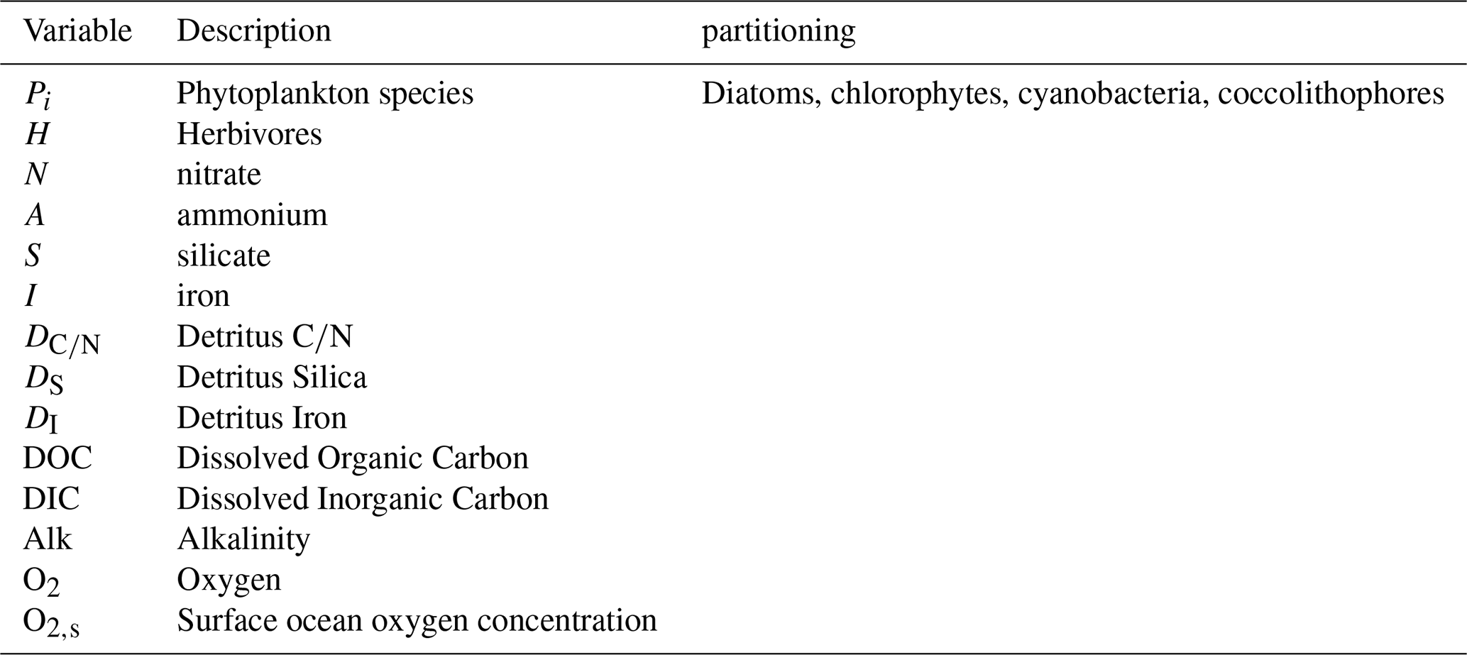
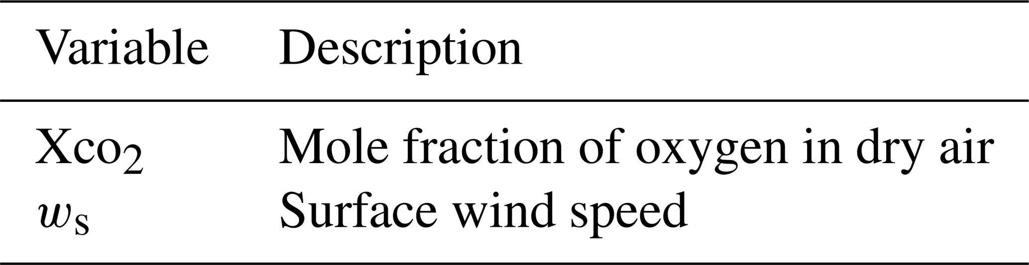
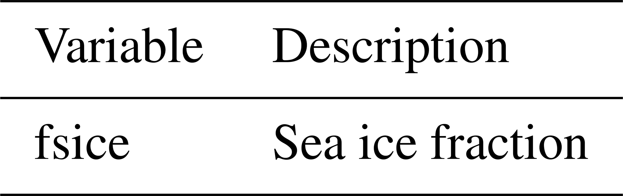
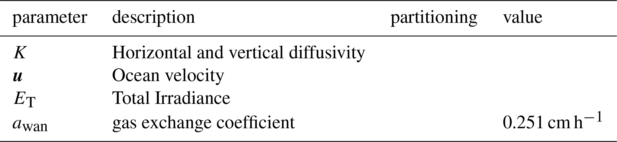
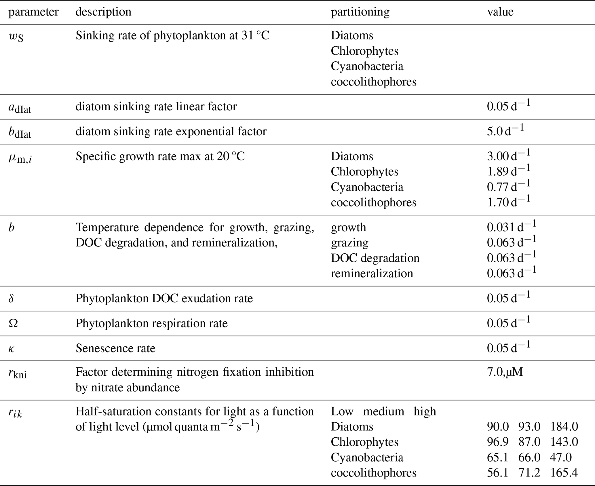
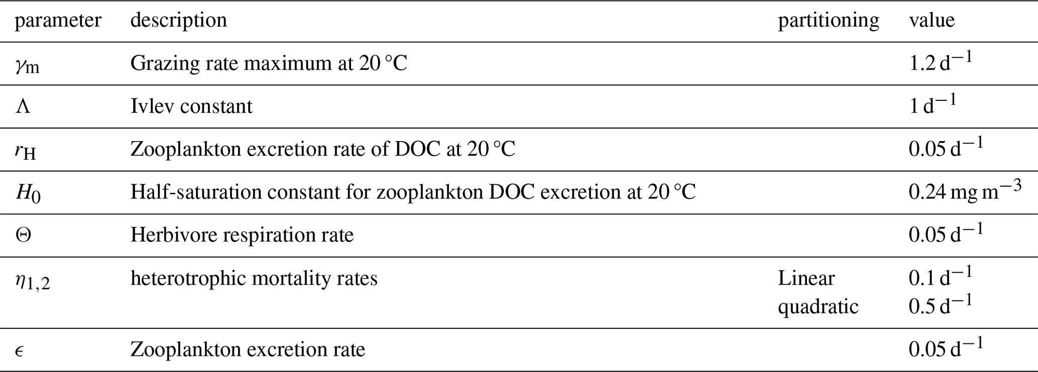
The nutrient dependent growth rates are:
where are half-saturation constants for nitrogen (ammonium and nitrate), iron, and silica limitation, respectively. Note that while kN remains set to the value used by Gregg and Casey (2007), kFe,Si have been adjusted as described in the section “Tuning”.
The temperature dependence of the growth rate is from Bissinger et al. (2008):
where the constant b, originally set to 0.0631 to fit phytoplankton data from the Liverpool Plankton Database, has been reduced to 0.031 to improve the regional distribution of net primary productivity (in particular, increase NPP in the subtropics). This also yields a Q10 of 1.36, which is closer to the Q10 obtained from a more recent compilation of phytoplankton community growth rates (1.47; Sherman et al., 2016) than the Q10 value found by Bissinger et al. (2008)
Specifically for cyanobacteria there is an additional temperature dependence which reduces their growth rate in cold waters (colder than 15 °C, Agawin et al., 1998, 2000).
Our treatment of nitrogen fixation, which amends the specific growth rate for cyanobacteria (second term in Eq. A2), has been revised from that of Gregg and Casey (2007), with two major differences. In Gregg and Casey (2007), the limitation of growth supported by nitrogen fixation included the same iron limitation (i.e., same half-saturation constant for iron-limitation of cyanobacteria) as non-nitrogen fixation supported growth. This has now been, i.e.:
where the half-saturation for iron limitation for nitrogen fixation (kFe,Nfix) was tuned to obtain a global nitrogen fixation rate that is within observational uncertainity, as described in the section “Tuning”.
Additionally, we have replaced the cyanobacterial biomass inhibition of nitrogen fixation with inhibition by the presence of nitrate and ammonium, following findings from laboratory studies using Trichodesmium cultures Holl and Montoya (2005). The inhibition factor (Nin,i) is set to 0 for all non-cyanobacteria remaining phytoplankton groups as these groups do not fix nitrogen and hence the term representing growth due to nitrogen fixation (second term in Eq. A2) is set to zero.
where rk,ni is the inhibition constant for nitrogen and ammonium from Holl and Monotya (2005).
Phytoplankton sinking is treated as additional vertical advection term (following Gregg and Casey, 2007) but with additional exponential dependence on diatom concentration for the diatoms and limiting term for coccolithophores which depends on the coccolithophore growth rate. For the other species is a function of viscosity (++++)
Note that gcmax, which is initialized to the value of the coccolithpohre growth rate, is updated each time step to either match the coccolithophore growth rate (if the growth rate is larger), or retain it's current value (if the growth rate larger).
Zooplankton grazing increases with temperature and the total biomass of phytoplankton.
where Λ and γm are the Ivlev constant and maximum grazing rate at 20 °C, respectively (Gregg and Casey, 2007).
Nutrients (nitrate, ammonium, silicate, iron)
The governing equation for nitrate is:
where the terms represent, from left to right, mixing, advection, uptake of nitrate via phytoplankton growth, detrital organic carbon nitrogen remineralization, and detrital organic carbon nitrogen breakdown to DOC. Here, bN is the nitrogen to chlorophyll ratio, C:N is the stoichiometric ratio of carbon to nitrogen in phytoplankton, and λD is the rate of detrital breakdown to DOC. Each of these parameters are set to the values in Gregg and Casey (2007). Note that R follows Eq. (A11) except that we retain b=0.0631 (the original value from Bissinger et al., 2008). αN, the remineralization rate of organic carbon nitrogen, follows:
where raer is the maximum rate of remineralization at 20 °C, H is the step function that equals 1 if O2 > 2 µmol kg−1, and 0 otherwise, and is the e-folding length scale for the oxygen-dependence of remineralization. The latter dependence was included following a study by Keil et al. (2016) that found the remineralization rate to decline exponentially with decreasing oxygen concentration (see also Lerner et al., 2024 for a discussion on how the value of was assigned).
, the fraction of nitrogen assimilated into phytoplankton biomass that is obtained from nitrate, follows:
The governing equation for ammonium is:
where the terms represent, from left to right, mixing, advection, uptake of ammonium via phytoplankton growth, and zooplankton excretion. Here, ϵ is the zooplankton excretion parameter, and , the fraction of nitrogen assimilated into phytoplankton biomass that is obtained from ammonium, follows:
The governing equation for dissolved silica is:
where the terms represent, from left to right, mixing, advection, uptake of silica via phytoplankton growth, dissolution of detrital silica. Here, bS is the silica to chlorophyll ratio, and αs is the detrital silica dissolution rate bS is set to the value in Gregg and Casey (2007), while αs was adjusted as described in the “Tuning” section. For dissolved iron, the governing equation is:
where the terms represent, from left to right, mixing, advection, uptake of iron via phytoplankton growth, zooplankton excretion, remineralization of detrital iron, atmospheric depiction, and the scavenging of ligand-bound and free iron. Here, bI is the iron to chlorophyll ratio, which is equal to the value used by Gregg and Casey (2007). αI, θ1, and θ2 are the remineralization rate, ligand-bound and free iron scavenging rates, respectively, whose values are adjusted as described in the “Tuning” section. AFe is the atmospheric deposition of iron bound to dust, which is prescribed as detailed in the “Forcings” section, while L is the thickness of the surface layer. I′ is solved for at each timestep from the system of equations that describe the complexation of iron with a single ligand class:
Ltot is from the prescribed ligand pool described in “Forcings.” The stability constant KFeL is set to a constant value of 1011 nmol L−1, taken from the average value from the compilation of Caprara et al. (2016).
Herbivores
The governing equations for herbivores is
where the terms represent, from left to right, mixing, advection, grazing, zooplankton linear and quadratic mortality, zooplankton excretion of DOC, and zooplankton respiration. Here, η1 and η2 are the linear and quadratic mortality rates, and Θ is the herbivore respiration rate. These constants are the same as those used by Gregg and Casey (2007). ζ is the excretion rate of DOC by herbivores, and follows:
where rH is the excretion rate of herbivores at 20 °C, and H0 is the half-saturation constant of herbivore excretion, both of which are set equal to the values from Gregg and Casey (2007). R is the temperature-dependence of herbivore excretion, which is equal to R for detrital nitrogen/carbon remineralization (Eq. A20).
Particulate organic components (carbon/nitrate detritus, silica detritus, iron detritus)
The governing equation for detrital carbon nitrogen is:
where the terms represent, from left to right, mixing, advection, sinking, remineralization of detrital iron, phytoplankton senescence, mortality of zooplankton, and breakdown of detrital carbon to DOC. Φ is the carbon to chlorophyll ratio, which is a constant value equal to the median (50 g C g chl−1) of the three values used to represent three photoadaptation states in Gregg and Casey (2007). αC is the remineralization rate of organic matter, defined as:
where raer is as defined in Eq. (A21), and rden is rate of remineralization at 20 °C under anaerobic conditions, where oxygen is no longer used as the terminal electron acceptor.
For detrital silica, the governing equation is:
where the terms represent, from left to right, mixing, advection, sinking, dissolution of detrital silica, phytoplankton senescence and herbivore grazing.
where the terms represent, from left to right, mixing, advection, sinking, remineralization of detrital iron, phytoplankton senescence, linear and quadratic herbivore mortality, and the scavenging of ligand-bound and free-iron.
For Eqs. (A32)–(A34), the detrital sinking rates follow and exponential dependence, similar to that for diatoms:
where the coefficients and have been previously described in Ito et al. (2020).
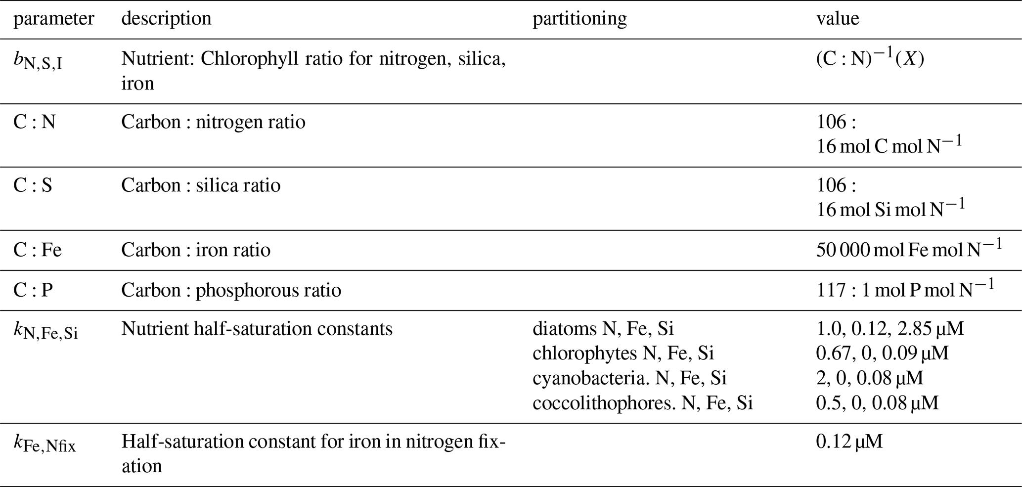
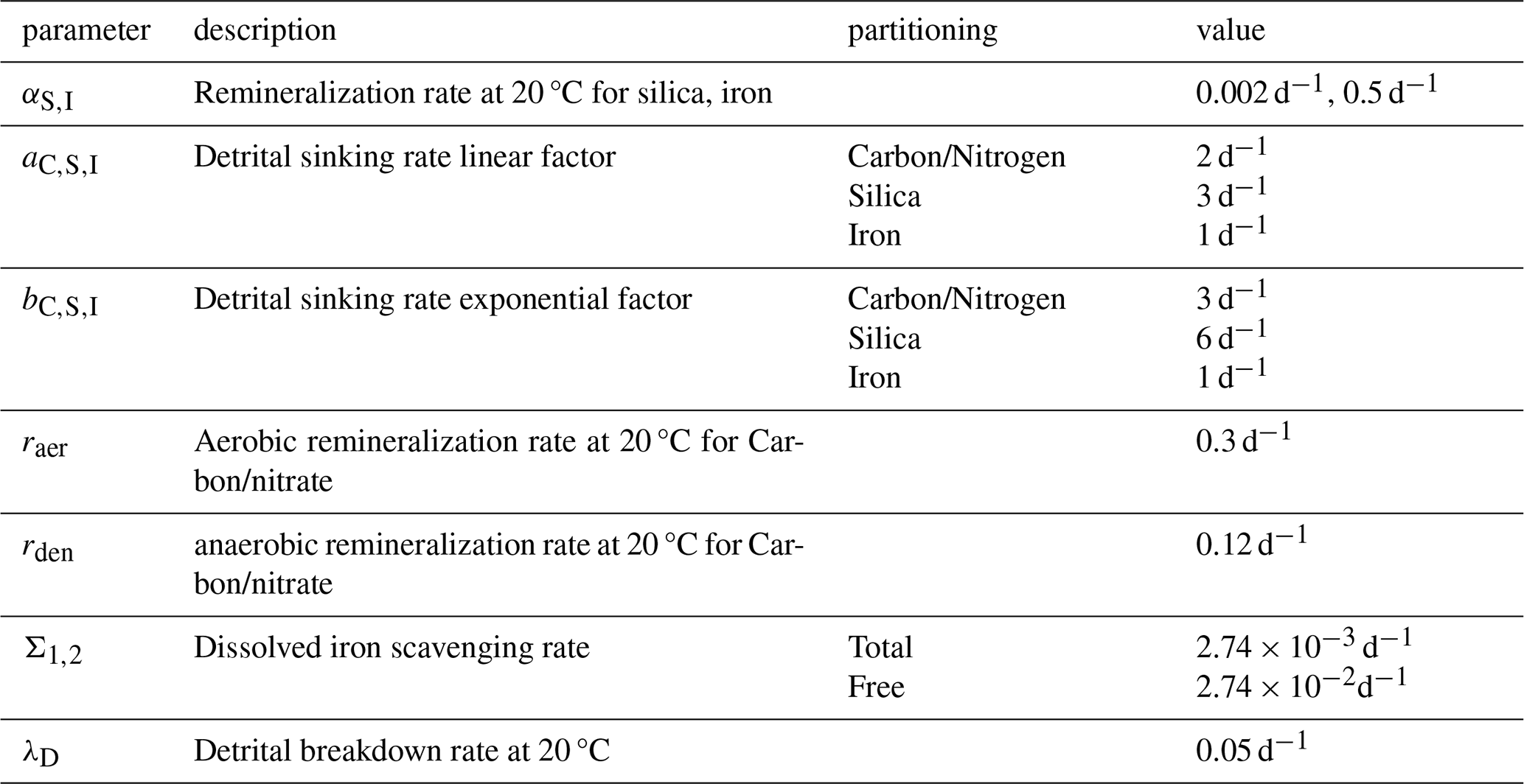
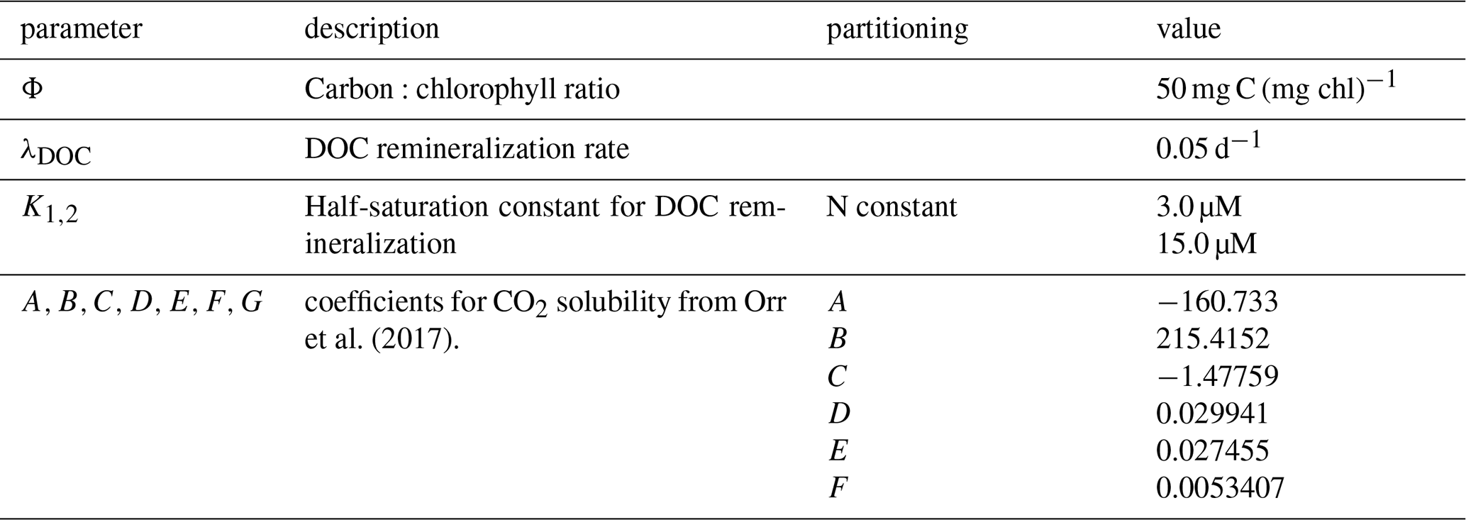
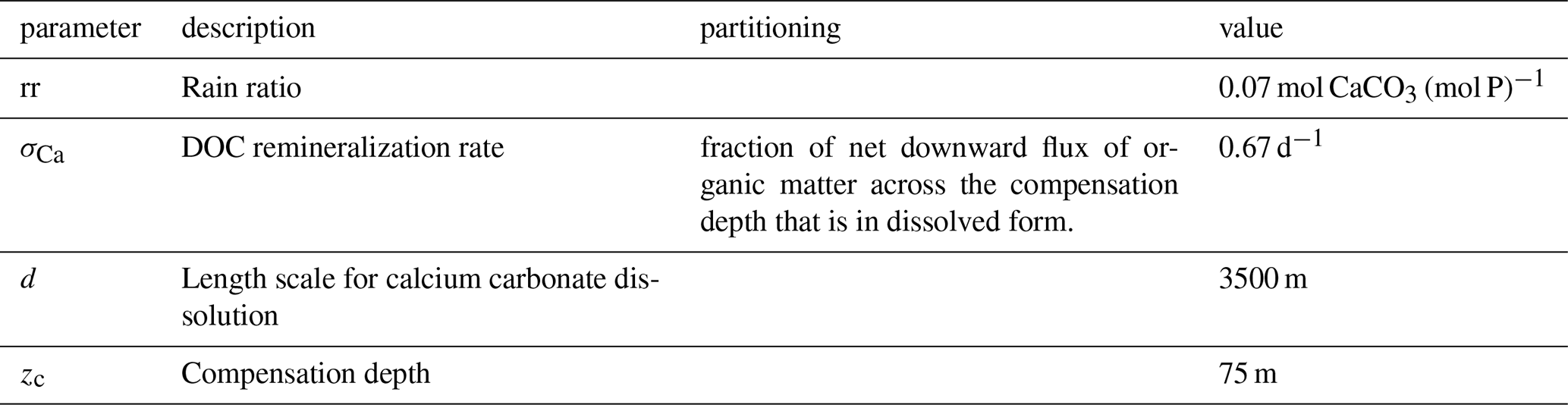
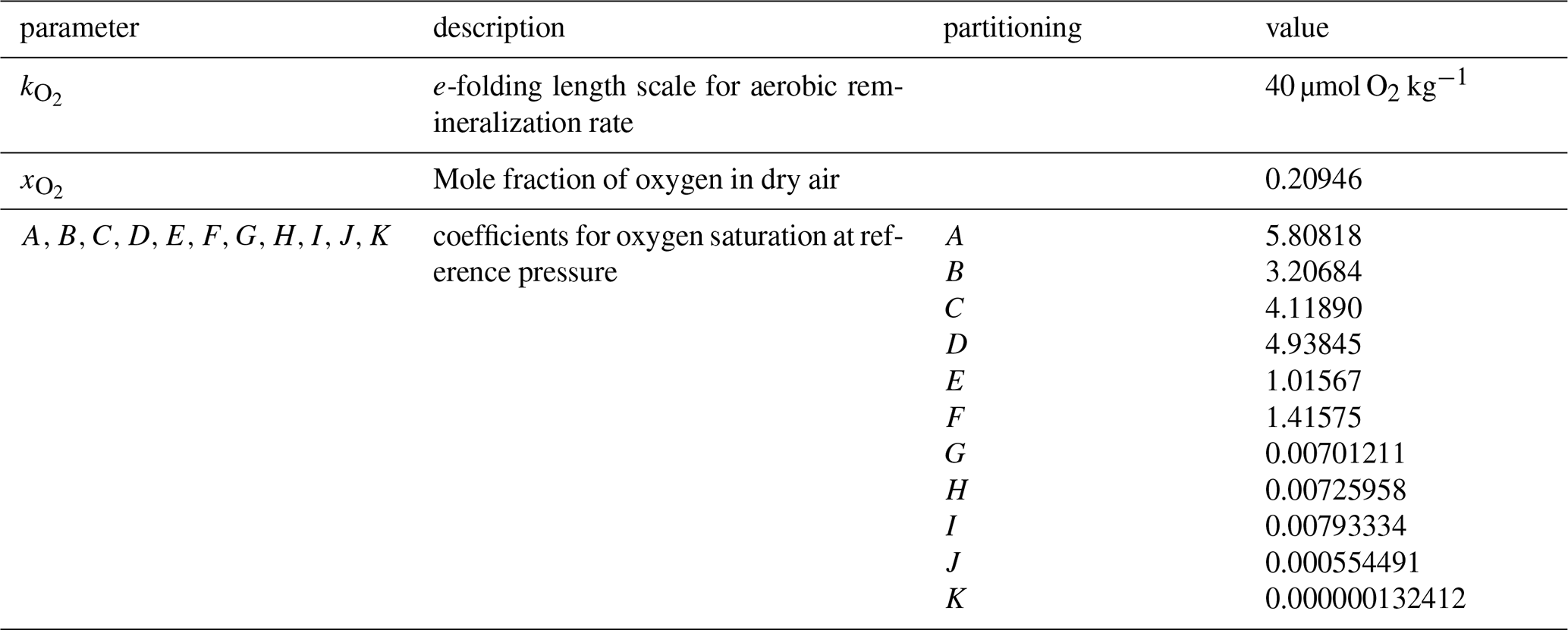

Carbon components (dissolved organic carbon, dissolved inorganic carbon, alkalinity)
The governing equation for dissolved organic carbon (DOC) is
where the terms represent, from left to right, mixing, advection, phytoplankton exudation, zooplankton excretion, breakdown of detrital carbon, and DOC remineralization. The DOC remineralization rate follows:
where H is the same step function used in Eq. (A21). λDOC is the maximum remineralization rate at 20 °C, and k1 and k2 are half-saturation constants for limitation of DOC remineralization by nitrogen and DOC, respectively. The constants are the same as those used by Gregg and Casey (2007). The temperature-dependent factor R follows the same parameterization as that used for the remineralization of detrital carbon nitrogen (Eq. A20).
The governing equation for dissolved inorganic carbon (DIC) is:
where the terms represent, from left to right, mixing, advection, uptake of DIC by phytoplankton, phytoplankton respiration, zooplankton respiration, DOC remineralization, detrital carbon remineralization, and the air-sea exchange of CO2. The last term follows the OMIP-BGC protocol for CMIP6 (Orr et al., 2017);
Where is the piston velocity of air-sea CO2 gas exchange, ff is the solubility of CO2, xCO2 is the dry-air fraction of atmospheric CO2 at the surface of the ocean, CO2,s is the partial pressure of CO2,s at the surface of the ocean, and fsice is the fraction of the surface ocean grid cell covered by sea ice. The piston velocity is computed following
Where awan is the Wanninkhof coefficient (Wanninkhof 2014, Orr et al., 2017), ws is the surface wind speed computed by the model, and is the Schmidt number that follows:
While the solubility of CO2 is computed following
Where tk, and the constant A–G are defined in Orr et al. (2017) (see also Table A9).
Alkalinity
The governing equation for alkalinity is:
where the terms represent, from left to right, mixing, advection, the increase in alkalinity due to the conversion of nitrate (a proton donor) to organic N, the decrease in alkalinity due to the conversion of organic N to nitrate during remineralization of detrital organic carbon nitrogen and DOC, and carbonate dissolution and precipitation. Carbonate dissolution and precipitation (JCa) follow the OCMIP-2 protocol:
Where rr is the rain ratio of CaCO3 to organic phosphorous (Yamanaka and Tajika, 1996), C:P is the organic carbon to organic phosphorous ratio, zc represents the compensation depth which we set to a constant value, and σCa is the fraction of calcium carbonate that dissolved within the compensation depth (Table A10). The change in the downward flux of calcium carbonate with depth uses a fixed exponential profile:
where d is a fixed exponential length scale for carbonate dissolution, and Fc is the primary productivity integrated from the surface to the compensation depth that is associated with the net production of calcium carbonate within the same depth interval:
PP is computed simply as the difference between the specific growth rate and the sum of respiration and exudation, integrated over all phytoplankton functional types:
Oxygen
The governing equation for dissolved oxygen is:
where the terms represent, from left to right, mixing, advection, production of O2 by phytoplankton, phytoplankton respiration, zooplankton respiration, DOC remineralization, detrital carbon remineralization, and the air-sea exchange of O2. bO and C:O are, respectively, the Redfield ratio of O2 produced or consumed by autotrophic and heterotrophic processes to chlorophyll and carbon in organic matter, respectively. As for CO2, The air-sea exchange of O2 follows the protocol described in Orr et al. (2017):
Where is the piston velocity for O2 exchange between the atmosphere and ocean, O2,sat is the O2 concentration at saturation, and O2,s is the surface concentration of O2. The piston velocity is computed following:
where is the Schmidt number of O2, which is computed following:
The O2 saturation concentration is also computed from the protocol of Orr et al. (2017):
where SLP is sea level pressure from the model, xO2 is the O2 dry-air air fraction, and the solubility coefficient Ksol is computed following:
where the partial pressure of H2O at the surface of the ocean is computed from model temperature and salinity:
And the saturation concentration of O2 at standard sea level pressure is computed following the equation of Garcia and Gordon (1992):
A2 Ent Terrestrial Biosphere Model
The complete formulation of the land carbon dynamics is given in Kim et al. (2015). In this study, prognostic growth is not turned on, but the vegetation model is run in “biophysics-only” mode, as described in Sect. 3.
B1 Köppen-Geiger classes
Table B1Köppen-Geiger biome/climate classes, with color scheme from http://koeppen-geiger.vu-wien.ac.at/ (last access: 21 August 2026).
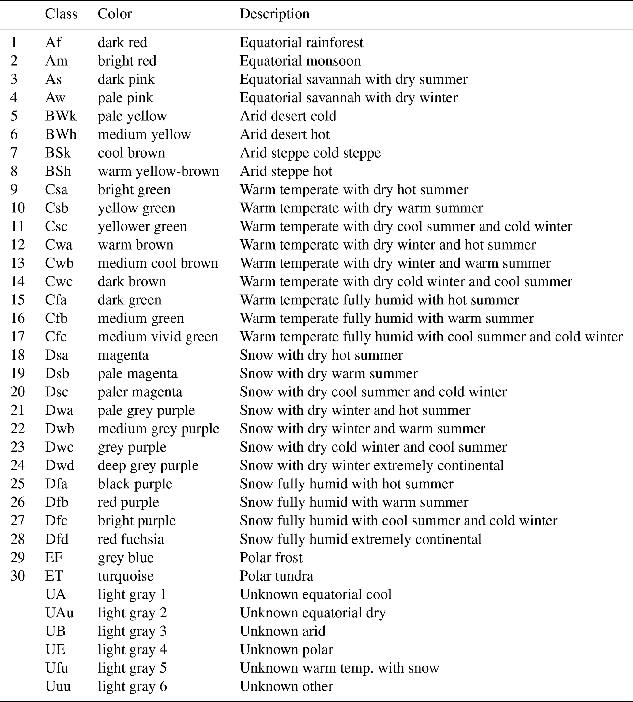
The current version of ModelE2.1-CC2 is available from the project website https://www.giss.nasa.gov/projects/gcm/ (last access: 21 August 2026). The exact version of the model used to produce the results used in this paper is archived on Zenodo under doi https://doi.org/10.5281/zenodo.17247307 (Romanou et al., 2025), as are input data and scripts to run the model and produce the plots for all the simulations presented in this paper.
The supplement related to this article is available online at https://doi.org/10.5194/gmd-19-9131-2026-supplement.
AR designed the structure of the paper, designed and run the simulations, developed scripts for the analysis, wrote the model description section and overall evaluation sections and had the general overview of the paper.
AR and PL run the simulations, developed scripts for the analysis of the results for all sections and contributed to the writing of the evaluations of the ocean carbon cycle.
PL developed scripts for the analysis and evaluation of the model and wrote the description of the ocean carbon cycle model and Appendix A1.
NK identified datasets for the land carbon model assessment, developed analysis scripts and wrote the relevant sections in the text.
IA assisted in setting up the full coupled cycle simulation.
MA is the main modelE developer and is responsible for updates in the physical climate model.
RLM provided support and guidance in coupling dust to the carbon cycle model and provided input in the text.
GR developed the carbon cycle conservation diagnostics and contributed to the model description and tuning sections.
RR is responsible for model diagnostic output, model running scripts and contributed to the model description sections.
GAS is responsible for the overall performance of modelE and contributed to the model description and tuning sections.
MAZ and OW contributed the ocean heat uptake and storage model evaluation datasets and the relevant writeup in the text.
The contact author has declared that none of the authors has any competing interests.
Publisher's note: Copernicus Publications remains neutral with regard to jurisdictional claims made in the text, published maps, institutional affiliations, or any other geographical representation in this paper. The authors bear the ultimate responsibility for providing appropriate place names. Views expressed in the text are those of the authors and do not necessarily reflect the views of the publisher.
We thank James Lui for assistance with processing land carbon and Fluxsat data and John Mekus for assistance in the analysis and the model simulations. Resources supporting this work were provided by the NASA High-End Computing (HEC) Program through the NASA Center for Climate Simulation (NCCS) at Goddard Space Flight Center.
AR, NYK, PL were supported by the NASA Modeling, Analysis, and Prediction (MAP) program. Contributing research by MH and OW was carried out at the Jet Propulsion Laboratory, California Institute of Technology, under a contract with the National Aeronautics and Space Administration (80NM0018D0004).
This paper was edited by Richard Neale and reviewed by two anonymous referees.
Abramopoulos, F., Rosenzweig, C., and Choudhury, B. J.: Improved ground hydrology calculations for global climate models (GCMs): soil water movement and evapotranspiration, J. Climate, 1, 921–941, 1988.
Adebiyi, A. A. and Kok, J. F.: Climate models miss most of the coarse dust in the atmosphere, Sci. Adv., 6, eaaz9507, https://doi.org/10.1126/sciadv.aaz9507, 2020.
Agawin, N. S., Duarte, C. M., and Agustí, S.: Nutrient and temperature control of the contribution of picoplankton to phytoplankton biomass and production, Limnol. Oceanogr., 45, 591–600, https://doi.org/10.4319/lo.2000.45.3.0591, 2000.
Anav, A., Friedlingstein, P., Beer, C., Ciais, P., Harper, A., Jones, C., Murray-Tortarolo, G., Papale, D., Parazoo, N. C., Peylin, P., Piao, S., Sitch, S., Viovy, N., Wiltshire, A., Zhao, M., Allen, R. J., Buchwitz, M., Guanter, L., Hantson, S., and Ichii, K.: Spatiotemporal patterns of terrestrial gross primary production: A review, Rev. Geophys., 53, 785–818, https://doi.org/10.1002/2015RG000483, 2015.
Armstrong, R. A., Lee, C., Hedges, J. I., Honjo, S., and Wakeham, S. G.: A new, mechanistic model for organic carbon fluxes in the ocean based on the quantitative association of POC with ballast minerals, Deep-Sea Res. Pt. II, 49, 219–236, https://doi.org/10.1016/S0967-0645(01)00101-1, 2001
Atwood, T. B., Romanou, A., DeVries, T., Lerner, P., Mayorga, J. S., Bradley, D., Cabral, R. B., Schmidt, G. A., and Sala, E.: Atmospheric CO2 emissions and ocean acidification from bottom-trawling, Front. Mar. Sci., 10, 1125137, https://doi.org/10.3389/fmars.2023.1125137, 2024.
Aumont, O., Ethé, C., Tagliabue, A., Bopp, L., and Gehlen, M.: PISCES-v2: an ocean biogeochemical model for carbon and ecosystem studies, Geosci. Model Dev., 8, 2465–2513, https://doi.org/10.5194/gmd-8-2465-2015, 2015.
Ball, J. T. and Berry, J. A.: A model predicting stomatal conductance and its contribution to photosynthesis under different environmental conditions. Progress in Photosynthesis Research. I, Biggins, Nijhoff, Dordrecht, Netherlands, IV, 110–112, https://doi.org/10.1007/978-94-017-0519-6_48, 1987.
Bastos, A., Sullivan, M., Ciais, P., Makowski, D., Sitch, S., Friedlingstein, P., Chevalier, F., Rodenbeck, C., Pongratz, J., Luijkx, I., Patra, P., Peylin, P., Canadell, J., Lauerwald, R., Li, W., Smith, N., Peters, W., Goll, D., Jain, A., Kato, E., Lienert, S., Lombardozzi, D., Haverd, V., Nabel, J., Tian, H., Walker, A., and Zaehle, S.: Aggregated regional estimates of net atmosphere-land CO2 fluxes from the five atmospheric inversions and 16 Dynamic Global Vegetation Models, supplemental data to Bastos et al., 2019 (https://doi.org/10.1029/2019GB006393), Integrated Carbon Observation System [data set], https://doi.org/10.18160/1SVH-3DNB, 2020.
Batjes, N. H.: Total carbon and nitrogen in the soils of the world, Eur. J. Soil Sci., 47, 151–163, 1996.
Berger, A. L.: Long-Term Variations of Daily Insolation and Quaternary Climatic Changes. J. Atmos. Sci., 35, 2362–2367, https://doi.org/10.1175/1520-0469(1978)035<2362:LTVODI>2.0.CO;2, 1978.
Bauer, S. E., Wright, D. L., Koch, D., Lewis, E. R., McGraw, R., Chang, L.-S., Schwartz, S. E., and Ruedy, R.: MATRIX (Multiconfiguration Aerosol TRacker of mIXing state): an aerosol microphysical module for global atmospheric models, Atmos. Chem. Phys., 8, 6003–6035, https://doi.org/10.5194/acp-8-6003-2008, 2008.
Bissinger, J. E., Montagnes, D. J., Harples, J., and Atkinson, D.: Predicting marine phytoplankton maximum growth rates from temperature: Improving on the Eppley curve using quantile regression, Limnol. Oceanogr., 53, 487–493, https://doi.org/10.4319/lo.2008.53.2.0487, 2008.
Bitz, C. M. and Lipscomb, W. H.: An energy-conserving thermodynamic model of sea ice. J. Geophys. Res.-Oceans, 104, 15669–15677, https://doi.org/10.1029/1999JC900100, 1999.
Brutsaert, W.: Evaporation into the Atmosphere: Theory, History, and Applications, Springer, Dordrecht, 299 pp., https://doi.org/10.1007/978-94-017-1497-6, 1982.
Buitenhuis, E. T., Pangerc, T., Franklin, D. J., Le Quéré, C., and Malin, G.: Growth rates of six coccolithophorid strains as a function of temperature, Limnol. Oceanogr., 53, 1181–1185, 2008.
Burd, A. B.: Modeling particle aggregation using size class and size spectrum approaches, J. Geophys. Res.-Oceans, 118, 3431–3443, https://doi.org/10.1002/jgrc.20255, 2013.
Cairns, B., Lacis, A. A., and Carlson, B. E.: Absorption within Inhomogeneous Clouds and Its Parameterization in General Circulation Models. J. Atmos. Sci., 57, 700–714, https://doi.org/10.1175/1520-0469(2000)057<0700:AWICAI>2.0.CO;2, 2000.
Cakmur, R. V., Miller, R. L., and Torres, O.: Incorporating the effect of small scale circulations upon dust emission in an AGCM, J. Geophys. Res., 109, D07201, https://doi.org/10.1029/2003JD004067, 2004.
Canadell, J. G., Monteiro, P. M. S., Costa, M. H., Cotrim da Cunha, L., Cox, P. M., Eliseev, A. V., Henson, S., Ishii, M., Jaccard, S., Koven, C., Lohila, A., Patra, P. K., Piao, S., Rogelj, J., Syampungani, S., Zaehle, S., and Zickfeld, K.: Global Carbon and Other Biogeochemical Cycles and Feedbacks, in: Climate Change 2021 – The Physical Science Basis: Working Group I Contribution to the Sixth Assessment Report of the Intergovernmental Panel on Climate Change, edited by: Masson-Delmotte, V., Zhai, P., Pirani, A., Connors, S. L., Péan, C., Berger, S., Caud, N., Chen, Y., Goldfarb, L., Gomis, M. I., Huang, M., Leitzell, K., Lonnoy, E., Matthews, J. B. R., Maycock, T. K., Waterfield, T., Yelekçi, O., Yu, R., and Zhou, B., (Cambridge University Press, Cambridge, 673–816, https://doi.org/10.1017/9781009157896.007, 2021.
Canuto, V. M. and Dubovikov, M. S.: A dynamical model for turbulence. I. General formalism, Phys. Fluids, 8, 571–585, https://doi.org/10.1063/1.868842, 1996a.
Canuto, V. M. and Dubovikov, M. S.: A dynamical model for turbulence. II. Shear-driven flows, Phys. Fluids, 8, 587-598, https://doi.org/10.1063/1.868843, 1996b.
Caprara, S., Buck, K. N., Gerringa, L. J., Rijkenberg, M. J., and Monticelli, D.: A compilation of iron speciation data for open oceanic waters, Front. Mar. Sci., 3, 221, https://doi.org/10.3389/fmars.2016.00221, 2016.
Castellanos, P., Colarco, P., Espinosa, W. R., Guzewich, S. D., Levy, R. C., Miller, R. L., Chin, M., Kahn, R. A., Kemppinen, O., Moosmüller, H., Nowottnick, E. P., Rocha-Lima, A., Smith, M. D., Yorks, J. E., and Yu, H.: Mineral dust optical properties for remote sensing and global modeling: A review, Remote Sens. Environ., 303, 113982, https://doi.org/10.1016/j.rse.2023.113982, 2024.
Chen, C.-T. and Millero, F. J.: The specific volume of seawater at high pressures, Deep-Sea Res., 23, 595–612, 1976.
Cheng, L., Zhang, L., Wang, Y.-P., Canadell, J. G., Chiew, F. H. S., Beringer, J., Li, L., Miralles, D. G., Piao, S., and Zhang, Y.: Recent increases in terrestrial carbon uptake at little cost to the water cycle, Nat. Commun., 8, 110, https://doi.org/10.1038/s41467-017-00114-5, 2017.
Cheng, Y., Canuto, V. M., and Howard, A. M.: An improved model for the turbulent PBL. J. Atmos. Sci., 59, 1550–1565, https://doi.org/10.1175/1520-0469(2002)059<1550:AIMFTT>2.0.co;2, 2002.
Coddington, O., Lean, J. L, Pilewskie, P., Snow, M., and Lindholm, D.: A Solar Irradiance Climate Data Record, B. Am. Meteorol. Soc., 97, 1265–1282, https://doi.org/10.1175/BAMS-D-14-00265.1, 2016.
Collatz, G. J., Ball, J. T., Grivet, C., and Berry, J. A.: Physiological and environmental regulation of stomatal conductance, photosynthesis and transpiration: a model that includes a laminar boundary layer, Agr. Forest Meteorol., 54, 107–136, 1991.
Collatz, M.-R. C. and Berry, J. A.: Coupled Photosynthesis-Stomatal Conductance Model for Leaves of C4 Plants, Austr. J. Plant Physiol., 19, 519–538, https://doi.org/10.1071/PP9920519, 1992.
Cook, B. I., Puma, M. J., and Krakauer, N. Y.: Irrigation induced surface cooling in the context of modern and increased greenhouse gas forcing, Clim. Dynam., 37, 1587–1600, https://doi.org/10.1007/s00382-010-0932-x, 2011.
Cook, B. I., Smerdon, J. E., Seager, R., and Coats, S.: Global warming and 21st century drying, Clim. Dynam., 43, 2607–2627, https://doi.org/10.1007/s00382-014-2075-y, 2014.
Cox, C. and Munk, W.: Slopes of the sea surface deduced from photographs of sun glitter, Bull. Scripps Inst. Oceanogr., 6, 401–488, 1956.
da Cunha, L. C., Buitenhuis, E. T., Le Quéré, C., Giraud, X., and Ludwig, W.: Potential impact of changes in river nutrient supply on global ocean biogeochemistry, Global Biogeochem. Cy., 21, https://doi.org/10.1029/2006GB002718, 2007.
Dale, A. W., Sommer, S., Ryabenko, E., Noffke, A., Bohlen, L., Wallmann, K., Stolpovsky, K., Greinert J., and Pfannkuche, O.: Benthic nitrogen fluxes and fractionation of nitrate in the Mauritanian oxygen minimum zone (Eastern Tropical North Atlantic), Geochim. Cosmochim. Ac., 134, 234–256, https://doi.org/10.1016/j.gca.2014.02.026, 2014.
DeVries, T.: The oceanic anthropogenic CO2 sink: Storage, air-sea fluxes, and transports over the industrial era, Global Biogeochem. Cy. 28, 631–647, https://doi.org/10.1002/2013GB004739, 2014.
Doney, S. C., Lindsay, K., Fung, I., and John, J.: Natural variability in a stable, 1000-yr global coupled climate-carbon cycle simulation, J. Climate, 19, 3033–3052, 2006.
Dubayah, R. O., Blair, J. B., Goetz, S., Fatoyinbo, L., Hansen, M., Healey, S., Hofton, M., Hurtt, G., Kellner, J., Luthcke, S., Armston, J., Tang, H., Duncanson, L., Hancock, S., Jantz, P., Marselis, S., Patterson, P. L., Qi, W., and Silva, C.: The Global Ecosystem Dynamics Investigation: High-resolution laser ranging of the Earth's forests and topography, Sci. Remote Sens., 1, 100002, https://doi.org/10.1016/j.srs.2020.100002, 2020.
Dubayah, R. O., Armston, J., Healey, S. P., Yang, Z., Patterson, P. L., Saarela, S., Stahl, G., Duncanson, L., and Kellner, J. R.: GEDI L4B Gridded Aboveground Biomass Density, Version 2, ORNL DAAC, Oak Ridge, Tennessee, USA [data set], https://doi.org/10.3334/ORNLDAAC/2017, 2022.
Erb, K. H., Kastner, T., Plutzar, C., Bais, A. L. S., Carvalhais, N., Fetzel, T., Gingrich, S., Haberl, H., Lauk, C., Niedertscheider, M., Pongratz, J., Thurner, M., and Luyssaert, S.: Unexpectedly large impact of forest management and grazing on global vegetation biomass, Nature, 553, 73–76, https://doi.org/10.1038/nature25138, 2018.
Farquhar, G. D. and von Caemmerer, S.: Modelling of Photosynthetic Response to Environmental Conditions, in: Physiological Plant Ecology II: Water Relations and Carbon Assimilation, edited by: Lange, O. L., Nobel, P. S., Osmond, C. B., and Ziegler, H., Berlin, Heidelberg, Springer Berlin Heidelberg, 549–587, https://doi.org/10.1007/978-3-642-68150-9_17, 1982.
Finkel, Z. V., Beardall, J., Flynn, K. J., Quigg, A., Rees, T. A. V., and Raven, J. A.: Phytoplankton in a changing world: cell size and elemental stoichiometry, J. Plank. Res., 32, 119–137, https://doi.org/10.1093/plankt/fbp098, 2010.
Forget, G., Campin, J.-M., Heimbach, P., Hill, C. N., Ponte, R. M., and Wunsch, C.: ECCO version 4: an integrated framework for non-linear inverse modeling and global ocean state estimation, Geosci. Model Dev., 8, 3071–3104, https://doi.org/10.5194/gmd-8-3071-2015, 2015.
Friedlingstein, P., O'Sullivan, M., Jones, M. W., Andrew, R. M., Hauck, J., Olsen, A., Peters, G. P., Peters, W., Pongratz, J., Sitch, S., Le Quéré, C., Canadell, J. G., Ciais, P., Jackson, R. B., Alin, S., Aragão, L. E. O. C., Arneth, A., Arora, V., Bates, N. R., Becker, M., Benoit-Cattin, A., Bittig, H. C., Bopp, L., Bultan, S., Chandra, N., Chevallier, F., Chini, L. P., Evans, W., Florentie, L., Forster, P. M., Gasser, T., Gehlen, M., Gilfillan, D., Gkritzalis, T., Gregor, L., Gruber, N., Harris, I., Hartung, K., Haverd, V., Houghton, R. A., Ilyina, T., Jain, A. K., Joetzjer, E., Kadono, K., Kato, E., Kitidis, V., Korsbakken, J. I., Landschützer, P., Lefèvre, N., Lenton, A., Lienert, S., Liu, Z., Lombardozzi, D., Marland, G., Metzl, N., Munro, D. R., Nabel, J. E. M. S., Nakaoka, S.-I., Niwa, Y., O'Brien, K., Ono, T., Palmer, P. I., Pierrot, D., Poulter, B., Resplandy, L., Robertson, E., Rödenbeck, C., Schwinger, J., Séférian, R., Skjelvan, I., Smith, A. J. P., Sutton, A. J., Tanhua, T., Tans, P. P., Tian, H., Tilbrook, B., van der Werf, G., Vuichard, N., Walker, A. P., Wanninkhof, R., Watson, A. J., Willis, D., Wiltshire, A. J., Yuan, W., Yue, X., and Zaehle, S.: Global Carbon Budget 2020, Earth Syst. Sci. Data, 12, 3269–3340, https://doi.org/10.5194/essd-12-3269-2020, 2020.
Friedlingstein, P., O'Sullivan, M., Jones, M. W., Andrew, R. M., Hauck, J., Landschützer, P., Le Quéré, C., Li, H., Luijkx, I. T., Olsen, A., Peters, G. P., Peters, W., Pongratz, J., Schwingshackl, C., Sitch, S., Canadell, J. G., Ciais, P., Jackson, R. B., Alin, S. R., Arneth, A., Arora, V., Bates, N. R., Becker, M., Bellouin, N., Berghoff, C. F., Bittig, H. C., Bopp, L., Cadule, P., Campbell, K., Chamberlain, M. A., Chandra, N., Chevallier, F., Chini, L. P., Colligan, T., Decayeux, J., Djeutchouang, L. M., Dou, X., Duran Rojas, C., Enyo, K., Evans, W., Fay, A. R., Feely, R. A., Ford, D. J., Foster, A., Gasser, T., Gehlen, M., Gkritzalis, T., Grassi, G., Gregor, L., Gruber, N., Gürses, Ö., Harris, I., Hefner, M., Heinke, J., Hurtt, G. C., Iida, Y., Ilyina, T., Jacobson, A. R., Jain, A. K., Jarníková, T., Jersild, A., Jiang, F., Jin, Z., Kato, E., Keeling, R. F., Klein Goldewijk, K., Knauer, J., Korsbakken, J. I., Lan, X., Lauvset, S. K., Lefèvre, N., Liu, Z., Liu, J., Ma, L., Maksyutov, S., Marland, G., Mayot, N., McGuire, P. C., Metzl, N., Monacci, N. M., Morgan, E. J., Nakaoka, S.-I., Neill, C., Niwa, Y., Nützel, T., Olivier, L., Ono, T., Palmer, P. I., Pierrot, D., Qin, Z., Resplandy, L., Roobaert, A., Rosan, T. M., Rödenbeck, C., Schwinger, J., Smallman, T. L., Smith, S. M., Sospedra-Alfonso, R., Steinhoff, T., Sun, Q., Sutton, A. J., Séférian, R., Takao, S., Tatebe, H., Tian, H., Tilbrook, B., Torres, O., Tourigny, E., Tsujino, H., Tubiello, F., van der Werf, G., Wanninkhof, R., Wang, X., Yang, D., Yang, X., Yu, Z., Yuan, W., Yue, X., Zaehle, S., Zeng, N., and Zeng, J.: Global Carbon Budget 2024, Earth Syst. Sci. Data, 17, 965–1039, https://doi.org/10.5194/essd-17-965-2025, 2025.
Fukumori, I., Wang, O., Fenty, I., Forget, G., Heimbach, P., and Ponte, R. M.: Synopsis of the ECCO Central Production Global Ocean and Sea-Ice State Estimate (Version 4 Release 4), Zenodo [code], https://doi.org/10.5281/zenodo.4533349, 2021.
Fung, I. Y., Meyn, S. K., Tegen, I., Doney, S. C., John, J. G., and Bishop, J. K. B.: Iron supply and demand in the upper ocean, Global Biogeochem. Cy., 14, 281–296, https://doi.org/10.1029/1999GB900059, 2000.
Garcia, H. E. and Gordon, L. I.: Oxygen solubility in seawater: Better fitting equations, Limnol. Oceanogr., 37, 1307–1312, https://doi.org/10.4319/lo.1992.37.6.1307, 1992.
Gao, F., Morisette, J. T., Wolfe, R. E., Ederer, G., Pedelty, J., Masuoka, E., Myneni, R., Tan, B. M., and Nightingale, J.: An algorithm to produce temporally and spatially continuous MODIS-LAI time series, IEEE Geosci. Remote Sens. Lett., 5, 60–64, https://doi.org/10.1109/LGRS.2007.907971, 2008.
Geider, R. J., MacIntyre H. L., and Kana, T. M.: A dynamic regulatory model of phytoplanktonic acclimation to light, nutrients, and temperature, Limnol. Oceanogr., 43, 679–694, 1998.
Gelaro, R., McCarty, W., Suárez, M. J., Todling, R., Molod, A., Takacs, L., Randles, C. A., Darmenov, A., Bosilovich, M. G., Reichle, R., Wargan, K., Coy, L., Cullather, R., Draper, C., Akella, S., Buchard, V., Conaty, A., da Silva, A. M., Gu, W., Kim, G.-K., Koster, R., Lucchesi, R., Merkova, D., Nielsen, J. E., Partyka, G., Pawson, S., Putman, W., Rienecker, M., Schubert, S. D., Sienkiewicz, M., and Zhao, B.: The Modern-Era Retrospective Analysis for Research and Applications, Version 2 (MERRA-2), J. Climate, 30, 5419–5454, https://doi.org/10.1175/JCLI-D-16-0758.1, 2017.
Gidden, M. J., Riahi, K., Smith, S. J., Fujimori, S., Luderer, G., Kriegler, E., van Vuuren, D. P., van den Berg, M., Feng, L., Klein, D., Calvin, K., Doelman, J. C., Frank, S., Fricko, O., Harmsen, M., Hasegawa, T., Havlik, P., Hilaire, J., Hoesly, R., Horing, J., Popp, A., Stehfest, E., and Takahashi, K.: Global emissions pathways under different socioeconomic scenarios for use in CMIP6: a dataset of harmonized emissions trajectories through the end of the century, Geosci. Model Dev., 12, 1443–1475, https://doi.org/10.5194/gmd-12-1443-2019, 2019.
Gill, A. E.: Atmosphere-Ocean Dynamics, Academic Press, 662 pp., 662 pp., ISBN 10 0-12-283520-4, 1982.
GISTEMP Team: GISS Surface Temperature Analysis (GISTEMP), version 4. NASA Goddard Institute for Space Studies, https://data.giss.nasa.gov/gistemp/ (last access: 28 September 2025), 2025.
Gordon, H. R. and Jacobs, M. M.: Albedo of the ocean–atmosphere system: influence of sea foam, Appl. Optics, 16, 2257–2260, https://doi.org/10.1364/AO.16.002257, 1977.
Grant, I., Ni-Meister, W., and Kiang, N. Y.: Multiscale analysis of global variation in tree allometric relationships: parameter sets for global vegetation models, Environ. Res.-Ecol., 4, 035002, https://doi.org/10.1088/2752-664X/add7e3, 2025.
Grant, S. R., Bienfang, P. K., and Laws, E. A.: Steady‐state bioassay approach applied to phosphorus‐limited continuous cultures: A growth study of the marine chlorophyte Dunaliella salina, Limnol. Oceanogr., 58, 314–324, 2013.
Gregg, W. W. and Casey, N. W.: Modeling coccolithophores in the global oceans, Deep-Sea Res. Pt. II, 54, 447–477, https://doi.org/10.1016/j.dsr2.2006.12.007, 2007.
Gregg, W. W. and Conkright, M. E.: Decadal changes in global ocean chlorophyll, Geophys. Res. Lett., 29, 201–204, https://doi.org/10.1029/2002GL014689, 2002.
Griffies, S. M.: The Gent–McWilliams Skew Flux, J. Phys. Oceanogr., 28, 831–841, https://doi.org/10.1175/1520-0485(1998)028<0831:TGMSF>2.0.co;2, 1998a.
Griffies, S. M., Gnanadesikan, A., Pacanowski, R. C., Larichev, V. D., Dukowicz, J. K., and Smith, R. D.: Isoneutral Diffusion in a z-Coordinate Ocean Model, J. Phys. Oceanogr., 28, https://doi.org/10.1175/1520-0485(1998)028<0805:IDIAZC>2.0.co;2, 1998b.
Hajima, T., Kawamiya, M., Ito, A., Tachiiri, K., Jones, C. D., Arora, V., Brovkin, V., Séférian, R., Liddicoat, S., Friedlingstein, P., and Shevliakova, E.: Consistency of global carbon budget between concentration- and emission-driven historical experiments simulated by CMIP6 Earth system models and suggestions for improved simulation of CO2 concentration, Biogeosciences, 22, 1447–1473, https://doi.org/10.5194/bg-22-1447-2025, 2025.
Hanninen, H. and Kramer, K.: A framework for modelling the annual cycle of trees in boreal and temperate regions, Silva Fenn., 41, 167–205, 2007.
Hansen, J., Russell, G., Rind, D., Stone, P., Lacis, A., Lebedeff, S., Ruedy, R., and Travis, L.: Efficient three-dimensional global models for climate studies: Models I and II, Mon. Weather Rev., 111, 609–662, https://doi.org/10.1175/1520-0493(1983)111<0609:ETDGMF>2.0.co;2, 1983.
Hansen, J., Sato, M., Ruedy, R., Kharecha, P., Lacis, A., Miller, R., Nazarenko, L., Lo, K., Schmidt, G. A., Russell, G., Aleinov, I., Bauer, S., Baum, E., Cairns, B., Canuto, V., Chandler, M., Cheng, Y., Cohen, A., del Genio, A., and Zhang, S.: Climate simulations for 1880-2003 with GISS ModelE, Clim. Dynam., 29, 661–696, https://doi.org/10.1007/s00382-007-0255-8, 2007.
Hartke, G. J. and Rind, D.: Improved surface and boundary layer models for the Goddard Institute for Space Studies general circulation model, J. Geophys. Res.-Atmos., 102, 16407–16422, https://doi.org/10.1029/97JD00698, 1997.
Heavens, N. G., Ward, D. S., and Mahowald, N. M.: Studying and Projecting Climate Change with Earth System Models, Nature Education Knowledge, 4, https://www.nature.com/scitable/knowledge/library/studying-and-projecting-climate-change-with-earth-103087065/ (last access: 21 August 2026), 2013.
Hegarty, T. W.: Temperature Coefficient (Q10), Seed Germination and Other Biological Processes, Nature, 243, 305–306, 1973.
Hersbach, H., Bell, B., Berrisford, P., Biavati, G., Horányi, A., Muñoz Sabater, J., Nicolas, J., Peubey, C., Radu, R., Rozum, I., Schepers, D., Simmons, A., Soci, C., Dee, D., and Thépaut, J-N: ERA5 monthly averaged data on single levels from 1940 to present, Copernicus Climate Change Service (C3S) Climate Data Store (CDS) [data set], https://doi.org/10.24381/cds.f17050d7, 2023.
Hirata, T., Hardman-Mountford, N. J., Brewin, R. J. W., Aiken, J., Barlow, R., Suzuki, K., Isada, T., Howell, E., Hashioka, T., Noguchi-Aita, M., and Yamanaka, Y.: Synoptic relationships between surface Chlorophyll-a and diagnostic pigments specific to phytoplankton functional types, Biogeosciences, 8, 311–327, https://doi.org/10.5194/bg-8-311-2011, 2011.
Hoesly, R. M., Smith, S. J., Feng, L., Klimont, Z., Janssens-Maenhout, G., Pitkanen, T., Seibert, J. J., Vu, L., Andres, R. J., Bolt, R. M., Bond, T. C., Dawidowski, L., Kholod, N., Kurokawa, J.-I., Li, M., Liu, L., Lu, Z., Moura, M. C. P., O'Rourke, P. R., and Zhang, Q.: Historical (1750–2014) anthropogenic emissions of reactive gases and aerosols from the Community Emissions Data System (CEDS), Geosci. Model Dev., 11, 369–408, https://doi.org/10.5194/gmd-11-369-2018, 2018.
Holl, C. M. and Montoya, J. P.: Interactions between nitrate uptake and nitrogen fixation in continuous cultures of the marine diazotroph Trichodesmium (cyanobacteria), J. Phycol., 41, 1178–1183, https://doi.org/10.1111/j.1529-8817.2005.00146.x, 2005.
Holtslag, A. A. M. and Boville, B. A.: Local Versus Nonlocal Boundary-Layer Diffusion in a Global Climate Model, J. Climate, 6, 1825–1842, https://doi.org/10.1175/1520-0442(1993)006<1825:LVNBLD>2.0.co;2, 1993.
Holtslag, A. A. M. and Moeng, C.-H.: Eddy Diffusivity and Countergradient Transport in the Convective Atmospheric Boundary Layer, J. Atmos. Sci., 48, 1690–1698, https://doi.org/10.1175/1520-0469(1991)048<1690:EDACTI>2.0.CO;2, 1991.
Holzer, M., DeVries, T., and de Lavergne, C.:. Diffusion controls the ventilation of a Pacific Shadow Zone above abyssal overturning, Nat. Commun., 12, 1–13, https://doi.org/10.1038/s41467-021-24648-x, 2021.
IES-1980, Millero, F. J., Poisson, A., Tung, C. C., Bradshaw, A. L., and Schleicher, K.: Background papers and supporting data on the International Equation of State of Seawater, 1980, Joint Panel on Oceanographic Tables and Standards, Sydney, Canada, UNESCO technical papers in marine science, 38, 192 pp., 1981.
Ito, G., Romanou, A., Kiang, N. Y., Faluvegi, G., Aleinov, I., Ruedy, R., Russell, G., Lerner, P., Kelley, M., and Lo, K.: Global Carbon Cycle and Climate Feedbacks in the NASA GISS ModelE2.1, J. Adv. Model. Earth Sy., 12, 1–44, https://doi.org/10.1029/2019MS002030, 2020.
Jacobson, A. R., Schuldt, K. N., Miller, J. B., Oda, T., Tans, P., Andrews, A., Mund, J., Ott, L., Collatz, G. J., Aalto, T., Afshar, S., Aikin, K., Aoki, S., Apadula, F., Baier, B., Bergamaschi, P., Beyersdorf, A., Biraud, S. C., and Bollenbacher, A.: CarbonTracker CT2022, NOAA Global Monitoring Laboratory, https://doi.org/10.25925/Z1GJ-3254, 2023.
Jayne, S. R.: The Impact of Abyssal Mixing Parameterizations in an Ocean General Circulation Model, J. Phys. Oceanogr., 39, 1756–1775, 10.1175/2009JPO4085.1, 2009.
Joiner, J. and Yoshida, Y.: Global MODIS and FLUXNET-derived Daily Gross Primary Production, V2, ORNL DAAC, Oak Ridge, Tennessee, USA [data set], https://doi.org/10.3334/ORNLDAAC/1835, 2021.
Jucker, T., Fischer, F. J., Chave, J., Coomes, D. A., Caspersen, J., Ali, A., Loubota Panzou, G. J., Feldpausch, T. R., Falster, D., Usoltsev, V. A., Adu-Bredu, S., Alves, L. F., Aminpour, M., Angoboy, I. B., Anten, N. P. R., Antin, C., Askari, Y., Muñoz, R., Ayyappan, N., Balvanera, P., Banin, L., Barbier, N., Battles, J. J., Beeckman, H., Bocko, Y. E., Bond-Lamberty, B., Bongers, F., Bowers, S., Brade, T., van Breugel, M., Chantrain, A., Chaudhary, R., Dai, J., Dalponte, M., Dimobe, K., Domec, J.-C., Doucet, J.-L., Duursma, R. A., Enríquez, M., van Ewijk, K. Y., Farfán-Rios, W., Fayolle, A., Forni, E., Forrester, D. I., Gilani, H., Godlee, J. L., Gourlet-Fleury, S., Haeni, M., Hall, J. S., He, J.-K., Hemp, A., Hernández-Stefanoni, J. L., Higgins, S. I., Holdaway, R. J., Hussain, K., Hutley, L. B., Ichie, T., Iida, Y., Jiang, H.-s., Joshi, P. R., Kaboli, H., Larsary, M. K., Kenzo, T., Kloeppel, B. D., Kohyama, T., Kunwar, S., Kuyah, S., Kvasnica, J., Lin, S., Lines, E. R., Liu, H., Lorimer, C., Loumeto, J.-J., Malhi, Y., Marshall, P. L., Mattsson, E., Matula, R., Meave, J. A., Mensah, S., Mi, X., Momo, S., Moncrieff, G. R., Mora, F., Nissanka, S. P., O'Hara, K. L., Pearce, S., Pelissier, R., Peri, P. L., Ploton, P., Poorter, L., Pour, M. J., Pourbabaei, H., Dupuy-Rada, J. M., Ribeiro, S. C., Ryan, C., Sanaei, A., Sanger, J., Schlund, M., Sellan, G., Shenkin, A., Sonké, B., Sterck, F. J., Svátek, M., Takagi, K., Trugman, A. T., Ullah, F., Vadeboncoeur, M. A., Valipour, A., Vanderwel, M. C., Vovides, A. G., Wang, W., Wang, L.-Q., Wirth, C., Woods, M., Xiang, W., Ximenes, F. d. A., Xu, Y., Yamada, T., and Zavala, M. A.: Tallo: A global tree allometry and crown architecture database, Glob. Change Biol., 28, 5254–5268, https://doi.org/10.1111/gcb.16302, 2022.
Kattge, J., Diaz, S., Lavorel, S., Prentice, C., Leadley, P., Bonisch, G., Garnier, E., Westoby, M., Reich, P. B., Wright, I. J., Cornelissen, J. H. C., Violle, C., Harrison, S. P., van Bodegom, P. M., Reichstein, M., Enquist, B. J., Soudzilovskaia, N. A., Ackerly, D. D., Anand, M., Atkin, O., Bahn, M., Baker, T. R., Baldocchi, D., Bekker, R., Blanco, C. C., Blonder, B., Bond, W. J., Bradstock, R., Bunker, D. E., Casanoves, F., Cavender-Bares, J., Chambers, J. Q., Chapin, F. S., Chave, J., Coomes, D., Cornwell, W. K., Craine, J. M., Dobrin, B. H., Duarte, L., Durka, W., Elser, J., Esser, G., Estiarte, M., Fagan, W. F., Fang, J., Fernandez-Mendez, F., Fidelis, A., Finegan, B., Flores, O., Ford, H., Frank, D., Freschet, G. T., Fyllas, N. M., Gallagher, R. V., Green, W. A., Gutierrez, A. G., Hickler, T., Higgins, S. I., Hodgson, J. G., Jalili, A., Jansen, S., Joly, C. A., Kerkhoff, A. J., Kirkup, D., Kitajima, K., Kleyer, M., Klotz, S., Knops, J. M. H., Kramer, K., Kuhn, I., Kurokawa, H., Laughlin, D., Lee, T. D., Leishman, M., Lens, F., Lenz, T., Lewis, S. L., Lloyd, J., Llusia, J., Louault, F., Ma, S., Mahecha, M. D., Manning, P., Massad, T., Medlyn, B. E., Messier, J., Moles, A. T., Muller, S. C., Nadrowski, K., Naeem, S., Niinemets, U., Nollert, S., Nuske, A., Ogaya, R., Oleksyn, J., Onipchenko, V. G., Onoda, Y., Ordonez, J., Overbeck, G., Ozinga, W. A., Patino, S., Paula, S., Pausas, J. G., Penuelas, J., Phillips, O. L., Pillar, V., Poorter, H., Poorter, L., Poschlod, P., Prinzing, A., Proulx, R., Rammig, A., Reinsch, S., Reu, B., Sack, L., Salgado-Negre, B., Sardans, J., Shiodera, S., Shipley, B., Siefert, A., Sosinski, E., Soussana, J. F., Swaine, E., Swenson, N., Thompson, K., Thornton, P., Waldram, M., Weiher, E., White, M., White, S., Wright, S. J., Yguel, B., Zaehle, S., Zanne, A. E., and Wirth, C.: TRY – a global database of plant traits, Glob. Change Biol., 17, 2905–2935, 10.1111/j.1365-2486.2011.02451.x, 2011.
Keil, R. G., Neibauer, J. A., Biladeau, C., van der Elst, K., and Devol, A. H.: A multiproxy approach to understanding the “enhanced” flux of organic matter through the oxygen-deficient waters of the Arabian Sea, Biogeosciences, 13, 2077–2092, https://doi.org/10.5194/bg-13-2077-2016, 2016.
Kelley, M., Schmidt, G. A., Nazarenko, L. S., Bauer, S. E., Ruedy, R., Russell, G. L., Ackerman, A. S., Aleinov, I., Bauer, M., Bleck, R., Canuto, V., Cesana, G., Cheng, Y., Clune, T. L., Cook, B. I., Cruz, C. A., del Genio, A. D., Elsaesser, G. S., Faluvegi, G., and Yao, M. S.: GISS-E2.1: Configurations and Climatology, J. Adv. Model. Earth Sy., 12, https://doi.org/10.1029/2019MS002025, 2020.
Kim, Y., Moorcroft, P. R., Aleinov, I., Puma, M. J., and Kiang, N. Y.: Variability of phenology and fluxes of water and carbon with observed and simulated soil moisture in the Ent Terrestrial Biosphere Model (Ent TBM version 1.0.1.0.0), Geosci. Model Dev., 8, 3837–3865, https://doi.org/10.5194/gmd-8-3837-2015, 2015.
Koster, R. D. and Suarez, M. J.: Energy and Water Balance Calculations in the Mosaic LSM (NASA Technical Memorandum 104606, Vol. 9; Technical Report Series on Global Modeling and Data Assimilation, 60 pp.). National Aeronautics and Space Administration, Goddard Space Flight Center, 1996.
Kopp, G. and Lean, J. L.: A new, lower value of total solar irradiance: Evidence and climate significance, Geophys. Res. Lett., 38, https://doi.org/10.1029/2010GL045777, 2011.
Kottek, M., Grieser, J., Beck, C., Rudolf, B., and Rubel, F.: World Map of the Köppen-Geiger climate classification updated, Meteorol. Z., 15, 259–263, https://doi.org/10.1127/0941-2948/2006/0130, 2006.
Krakauer, N. Y., Puma, M. J., Cook, B. I., Gentine, P., and Nazarenko, L.: Ocean–atmosphere interactions modulate irrigation's climate impacts, Earth Syst. Dynam., 7, 863–876, https://doi.org/10.5194/esd-7-863-2016, 2016.
Krumhardt, K. M., Lovenduski, N. S., Iglesias-Rodriguez, M. D., and Kleypas, J. A.: Coccolithophore growth and calcification in a changing ocean, Progr. Oceanogr., 159, 276–295, https://doi.org/10.1016/j.pocean.2017.10.007, 2017.
Lacis, A. A. and Oinas, V.: A description of the correlated k distribution method for modeling nongray gaseous absorption, thermal emission, and multiple scattering in vertically inhomogeneous atmospheres, J. Geophys. Res.-Atmos., 96, 9027–9063, https://doi.org/10.1029/90JD01945, 1991.
Landschützer, P., Gruber, N., and Bakker, D. C. E.: Decadal variations and trends of the globalocean carbon sink, Global Biogeochem. Cy., 30, 1396–1417, https://doi.org/10.1002/2015GB005359, 2016.
Lam, P. and Kuypers, M. M. Microbial nitrogen cycling processes in oxygen minimum zones, Annu. Rev. Mar. Sci., 3, 317–345, https://doi.org/10.1146/annurev-marine-120709-142814, 2011.
Lan, X., Tans, P., and Thoning, K. W.: Trends in globally-averaged CO2 determined from NOAA Global Monitoring Laboratory measurements [data set], https://doi.org/10.15138/9N0H-ZH07, 2022a.
Lan, X., Thoning, K. W., and Dlugokencky, E. J.: Trends in globally-averaged CH4, N2O, and SF6 determined from NOAA Global Monitoring Laboratory measurements [data set], https://doi.org/10.15138/P8XG-AA10, 2022b.
Large, W. G., McWilliams, J. C., and Doney, S. C.: Oceanic vertical mixing: A review and a model with a nonlocal boundary layer parameterization, Rev. Geophys., 32, 363–403, https://doi.org/10.1029/94RG01872, 1994.
Latto, R. and Romanou, A.: The Ocean Carbon States Database: a proof-of-concept application of cluster analysis in the ocean carbon cycle, Earth Syst. Sci. Data, 10, 609–626, https://doi.org/10.5194/essd-10-609-2018, 2018.
Lauvset, S. K., Key, R. M., Olsen, A., van Heuven, S., Velo, A., Lin, X., Schirnick, C., Kozyr, A., Tanhua, T., Hoppema, M., Jutterström, S., Steinfeldt, R., Jeansson, E., Ishii, M., Perez, F. F., Suzuki, T., and Watelet, S.: A new global interior ocean mapped climatology: the 1° × 1° GLODAP version 2, Earth Syst. Sci. Data, 8, 325–340, https://doi.org/10.5194/essd-8-325-2016, 2016.
Lawrence, D., Thornton, P. E., Oleson, K. W., and Bonan, G. B.: The partitioning of evapotranspiration into transpiration, soil evaporation, and canopy evaporation in a GCM: Impacts on land-atmosphere interaction, J. Hydrometeorol., 8, 862–880, https://doi.org/10.1175/JHM596.1, 2007.
Laws, E. A., Pei, S., Bienfang, P., and Grant, S.: Phosphate-limited growth and uptake kinetics of the marine prasinophyte Tetraselmis suecica (Kylin) Butcher, Aquaculture, 322, 117-121, https://doi.org/10.1016/j.aquaculture.2011.09.041, 2011.
Lennsen, N., Schmidt, G. A., Hendrickson, M., Jacobs, P., Menne, M., and Ruedy, R.: A GISTEMPv4 observational uncertainty ensemble, J. Geophys. Res.-Atmos., 129, 1–18, https://doi.org/10.1029/2023JD040179, 2024.
Lerner, P., Marchal, O., Lam, P. J., Buesseler, K., and Charette, M.: Kinetics of thorium and particle cycling along the US GEOTRACES North Atlantic Transect, Deep-Sea Res. Pt. I, 125, 106–128, https://doi.org/10.1016/j.dsr.2017.05.003, 2017.
Lerner, P., Romanou, A., Kelley, M., Romanski, J., Ruedy, R., and Russell, G.: Drivers of air-sea CO2 flux seasonality and its long-term changes in the NASA-GISS model CMIP6 submission, J. Adv. Model. Earth Sy., 13, e2019MS002028, https://doi.org/10.1029/2019MS002028, 2021.
Lerner, P., Romanou, A., Nicholson, D., Kelley, M., Ruedy, R., and Russell, G.: The sensitivity of the Equatorial Pacific ODZ to particulate organic matter remineralization in a climate model under pre-industrial conditions, Ocean Model., 188, 102303, https://doi.org/10.1016/j.ocemod.2023.102303, 2024.
Levis, S., Bonan, G. B., Vertenstein, M., and Oleson, K. W.: The Community Land Model’s Dynamic Global Vegetation Model (CLM-DGVM): Technical Description and User’s Guide (NCAR Technical Note NCAR/TN-459+STR), Terrestrial Sciences Section, Climate and Global Dynamics Division, National Center for Atmospheric Research, Boulder, CO, 2004.
Liefer, J. D., Garg, A., Campbell, D. A., Irwin, A. J., and Finkel, Z. V.: Nitrogen starvation induces distinct photosynthetic responses and recovery dynamics in diatoms and prasinophytes, PLoS One, 13, e0195705, https://doi.org/10.1371/journal.pone.0195705, 2018.
Liu, G., Ciais, P., Tao, S., Yang, H., and Bastos, A.: A High-Resolution, Long-Term Global Radar-Based Above-Ground Biomass Dataset from 1993 to 2020, Earth Syst. Sci. Data Discuss. [preprint], https://doi.org/10.5194/essd-2025-330, 2025.
Locarnini, R. A., Mishonov, A. V., Baranova, O. K., Reagan, J. R., Boyer, T. P., Seidov, D., Wang, Z., Garcia, H. E., Bouchard, C., Cross, S. L., Paver, C. R., and Dukhovskoy, D.: World Ocean Atlas 2023, Volume 1: Temperature, NOAA Atlas NESDIS 89, 40 pp., https://doi.org/10.25923/54bh-1613, 2024.
Loth, B., and Graf, H.-F.: Modeling the snow cover in climate studies: 1. Long-term integrations under different climatic conditions using a multilayered snow-cover model, J. Geophys. Res.-Atmos., 103, 11313–11327, https://doi.org/10.1029/97JD01411, 1998.
Lyman, J. M. and Johnson, G. C.: Global High-Resolution Random Forest Regression Maps of Ocean Heat Content Anomalies Using in Situ and Satellite Data, J. Atmos. Ocean. Tech., https://doi.org/10.1175/JTECH-D-22-0058.1, 2023.
Makela, A., Hari, P., Berninger, F., Hanninen, H., and Nikinmaa, E.: Acclimation of photosynthetic capacity in Scots pine to the annual cycle of temperature, Tree Physiol., 24, 369–376, 2004.
Makela, A., Kolari, P. J., Karimaki, E., Nikinmaa, M., Peramaki, M., and Hari, P.: Modelling five years of weather-driven variation of GPP in a boreal forest, Agr. Forest Meteorol., 139, 382–398, 2006.
Marshall, J., Scott, J. R., Romanou, A., Kelley, M., and Leboissetier, A.: The dependence of the ocean's MOC on mesoscale eddy diffusivities: A model study, Ocean Model., 111, 1–8, https://doi.org/10.1016/j.ocemod.2017.01.001, 2017.
Massoud, E. C., Xu, C., Fisher, R. A., Knox, R. G., Walker, A. P., Serbin, S. P., Christoffersen, B. O., Holm, J. A., Kueppers, L. M., Ricciuto, D. M., Wei, L., Johnson, D. J., Chambers, J. Q., Koven, C. D., McDowell, N. G., and Vrugt, J. A.: Identification of key parameters controlling demographically structured vegetation dynamics in a land surface model: CLM4.5(FATES), Geosci. Model Dev., 12, 4133–4164, https://doi.org/10.5194/gmd-12-4133-2019, 2019.
Matthews, E.: Prescription of land-surface boundary conditions in GISS GCM II: A simple method based on high-resolution vegetation data bases (NASA Technical Memorandum 86096), National Aeronautics and Space Administration, Goddard Institute for Space Studies, 1984.
Matthes, K., Funke, B., Andersson, M. E., Barnard, L., Beer, J., Charbonneau, P., Clilverd, M. A., Dudok de Wit, T., Haberreiter, M., Hendry, A., Jackman, C. H., Kretzschmar, M., Kruschke, T., Kunze, M., Langematz, U., Marsh, D. R., Maycock, A. C., Misios, S., Rodger, C. J., Scaife, A. A., Seppälä, A., Shangguan, M., Sinnhuber, M., Tourpali, K., Usoskin, I., van de Kamp, M., Verronen, P. T., and Versick, S.: Solar forcing for CMIP6 (v3.2), Geosci. Model Dev., 10, 2247–2302, https://doi.org/10.5194/gmd-10-2247-2017, 2017.
Meinshausen, M., Vogel, E., Nauels, A., Lorbacher, K., Meinshausen, N., Etheridge, D. M., Fraser, P. J., Montzka, S. A., Rayner, P. J., Trudinger, C. M., Krummel, P. B., Beyerle, U., Canadell, J. G., Daniel, J. S., Enting, I. G., Law, R. M., Lunder, C. R., O'Doherty, S., Prinn, R. G., Reimann, S., Rubino, M., Velders, G. J. M., Vollmer, M. K., Wang, R. H. J., and Weiss, R.: Historical greenhouse gas concentrations for climate modelling (CMIP6), Geosci. Model Dev., 10, 2057–2116, https://doi.org/10.5194/gmd-10-2057-2017, 2017.
Mellor, G. L. and Yamada, T.: Development of a turbulence closure model for geophysical fluid problems, Rev. Geophys., 20, 851–875, https://doi.org/10.1029/RG020i004p00851, 1982.
Meng, J., Huang, Y., Leung, D. M., Li, L., Adebiyi, A. A., Ryder, C. L., Mahowald, N. M., and Kok, J. F.: Improved parameterization for the size distribution of emitted dust aerosols reduces model underestimation of super coarse dust, Geophys. Res. Lett., 49, e2021GL097287, https://doi.org/10.1029/2021GL097287, 2022.
Mezuman, K., Tsigaridis, K., Faluvegi, G., and Bauer, S. E.: The interactive global fire module pyrE (v1.0), Geosci. Model Dev., 13, 3091–3118, https://doi.org/10.5194/gmd-13-3091-2020, 2020.
Miller, R. L., Cakmur, R. V., Perlwitz, J. P., Geogdzhayev, I. V., Ginoux, P., Kohfeld, K. E., Koch, D., Prigent, C., Ruedy, R., Schmidt, G. A., and Tegen, I.: Mineral dust aerosols in the NASA Goddard Institute for Space Sciences ModelE atmospheric general circulation model, J. Geophys. Res., 111, D06208, https://doi.org/10.1029/2005JD005796, 2006.
Miller, R. L., Schmidt, G. A., Nazarenko, L. S., Bauer, S. E., Kelley, M., Ruedy, R., Russell, G. L., Ackerman, A. S., Aleinov, I., Bauer, M., Bleck, R., Canuto, V., Cesana, G., Cheng, Y., Clune, T. L., Cook, B. I., Cruz, C. A., del Genio, A. D., Elsaesser, G. S., and Yao, M. S.: CMIP6 Historical Simulations (1850–2014) With GISS-E2.1, J. Adv. Model. Earth Sy., 13, 1–59, https://doi.org/10.1029/2019MS002034, 2021.
Mishchenko, M. I., Travis, L. D., and Mackowski, D. W.: T-matrix computations of light scattering by nonspherical particles: A review, J. Quant. Spectrosc. Ra., 55, 535–575, https://doi.org/10.1016/0022-4073(96)00002-7, 1996.
Myneni, R. B., Hoffman, S., Knyazikhin, Y., Privette, J. L., Glassy, J., Tian, Y., Wang, Y., Song, X., Zhang, Y., Smith, G. R., Lotsch, A., Friedl, M., Morisette, J. T., Votava, P., Nemani, R. R., and Running, S. W.: Global products of vegetation leaf area and fraction absorbed PAR from year one of MODIS data, Remote Sens. Environ., 83, 214–231, 2002.
Najjar, R. G., Jin, X., Louanchi, F., Aumont, O., Caldeira, K., Doney, S. C., Dutay, J.-C., Follows, M., Gruber, N., Joos, F., Lindsay, K., Maier-Reimer, E., Matear, R. J., Matsumoto, K., Monfray, P., Mouchet, A., Orr, J. C., Plattner, G.-K., Sarmiento, J. L., Schlitzer, R., Slater, R. D., Weirig, M.-F., Yamanaka, Y., and Yool, A.: Impact of circulation on export production, dissolved organic matter, and dissolved oxygen in the ocean: Results from Phase II of the Ocean Carbon-cycle Model Intercomparison Project (OCMIP-2), Global Biogeochem. Cy., 21, https://doi.org/10.1029/2006GB002857, 2007.
Nakanishi, M.: Improvement of the Mellor–Yamada turbulence closure model based on large eddy simulation data, Bound.-Lay. Meteorol., 99, 349–378, https://doi.org/10.1023/A:1018915827400, 2001.
Nelson, D. M. and Tréguer, P.: Role of silicon as a limiting nutrient to Antarctic diatoms: evidence from kinetic studies in the Ross Sea ice-edge zone, Mar. Ecol. Prog. Ser., 80, 255–264, https://doi.org/10.3354/meps080255, 1992.
Ni-Meister, W., Yang, W. Z., and Kiang, N. Y.: A clumped-foliage canopy radiative transfer model for a global dynamic terrestrial ecosystem model. I: Theory, Agr. Forest Meteorol., 150, 881–894, https://doi.org/10.1016/j.agrformet.2010.02.009, 2010.
Ochoa, F., Brodrick, P. G., Okin, G. S., Ben-Dor, E., Meyer, T., Thompson, D. R., and Green, R. O.: Soil and vegetation cover estimation for global imaging spectroscopy using spectral mixture analysis, Remote Sens. Environ., 324, 114746, https://doi.org/10.1016/j.rse.2025.114746, 2025.
Oinas, V., Lacis, A. A., Rind, D., Shindell, D. T., and Hansen, J. E.: Radiative cooling by stratospheric water vapor: Big differences in GCM results, Geophys. Res. Lett., 28, 2791–2794, https://doi.org/10.1029/2001GL013137, 2001.
Orr, J. C. and Epitalon, J.-M.: Improved routines to model the ocean carbonate system: mocsy 2.0, Geosci. Model Dev., 8, 485–499, https://doi.org/10.5194/gmd-8-485-2015, 2015.
Orr, J. C., Najjar, R. G., Aumont, O., Bopp, L., Bullister, J. L., Danabasoglu, G., Doney, S. C., Dunne, J. P., Dutay, J.-C., Graven, H., Griffies, S. M., John, J. G., Joos, F., Levin, I., Lindsay, K., Matear, R. J., McKinley, G. A., Mouchet, A., Oschlies, A., Romanou, A., Schlitzer, R., Tagliabue, A., Tanhua, T., and Yool, A.: Biogeochemical protocols and diagnostics for the CMIP6 Ocean Model Intercomparison Project (OMIP), Geosci. Model Dev., 10, 2169–2199, https://doi.org/10.5194/gmd-10-2169-2017, 2017.
Parekh, P., Follows, M. J., and Boyle, E.: Modeling the global ocean iron cycle, Global Biogeochem. Cy., 18, 1–5, https://doi.org/10.1029/2003GB002061, 2004.
Pérez García-Pando, C., Miller, R. L., Perlwitz, J. P., Rodríguez, S., and Prospero, J. M.: Predicting the mineral composition of dust aerosols: Insights from elemental composition measured at the Izaña Observatory, Geophys. Res. Lett., 43, 10520–10529, https://doi.org/10.1002/2016GL069873, 2016.
Perlwitz, J. P., Pérez García-Pando, C., and Miller, R. L.: Predicting the mineral composition of dust aerosols – Part 1: Representing key processes, Atmos. Chem. Phys., 15, 11593–11627, https://doi.org/10.5194/acp-15-11593-2015, 2015a.
Perlwitz, J. P., Pérez García-Pando, C., and Miller, R. L.: Predicting the mineral composition of dust aerosols – Part 2: Model evaluation and identification of key processes with observations, Atmos. Chem. Phys., 15, 11629–11652, https://doi.org/10.5194/acp-15-11629-2015, 2015b.
Potter, C. S., Matson, P. A., and Vitousek, P. M.: Process modeling of controls on nitrogen trace gas emissions from soils worldwide, J. Geophys. Res., 101, 1361–1377, 1996.
Prather, M. J.: Numerical advection by conservation of second-order moments, J. Geophys. Res.-Atmos., 91, 6671–6681, https://doi.org/10.1029/JD091iD06p06671, 1986.
Puma, M. J. and Cook, B. I.: Effects of irrigation on global climate during the 20th century, J. Geophys. Res., 115, D16120, https://doi.org/10.1029/2010JD014122, 2010.
Quigley, M. S., Santschi, P. H., Hung, C. C., Guo, L., and Honeyman, B. D.: Importance of acid polysaccharides for 234Th complexation to marine organic matter, Limnol. Oceanogr., 47, 367–377, https://doi.org/10.4319/lo.2002.47.2.0367, 2002.
Randerson, J. T., Hoffman, F. M., Thornton, P. E., Mahowald, N. M., Lindsay, K., Lee, Y. H., Nevison, C. D., Doney, S. C., Bonan, G., Stockli, R., Covey, C., Running, S. W., and Fung, I. Y.: Systematic assessment of terrestrial biogeochemistry in coupled climate-carbon models, Glob. Change Biol., 15, 2462–2484, 2009.
Randerson, J. T., Li, Y., Fu, W., Primeau, F., Kim, J. E., Mu, M., Hoffman, F. M., Trugman, A. T., Yang, L., Wu, C., Wang, J. A., Anderegg, W. R. L., Baccini, A., Friedl, M. A., Saatchi, S. S., Denning, A. S., and Goulden, M. L.: The weak land carbon sink hypothesis, Sci. Adv., 11, eadr5489, https://doi.org/10.1126/sciadv.adr5489, 2025.
Reagan, J. R., Seidov, D., Wang, Z., Dukhovskoy, D., Boyer, T. P., Locarnini, R. A., Baranova, O. K., Mishonov, A. V., Garcia, H. E., Bouchard, C., Cross, S. L., and Paver, C. R.: World Ocean Atlas 2023, Volume 2: Salinity. A. Mishonov, Technical Editor, NOAA Atlas NESDIS 90, 52 pp., https://doi.org/10.25923/70qt-9574, 2024.
Repo, T., Makela, A., and Hanninen, H. (Eds.): Modelling to understand forest functions, Silva Carelica, 15, 61–74, University of Joensuu, ISBN-10 951-696-891-0,10, 1990.
Respati, M. R., Dommenget, D., Segura, H., and Stassen, C.: Diagnosing drivers of tropical precipitation biases in coupled climate model simulations, Clim. Dynam., 62, 8691–8709, 10.1007/s00382-024-07355-3, 2024.
Rodriguez-Iturbe, I., Porporato, A., Laio, F., and Ridolfi, L.: Plants in water-controlled ecosystems: active role in hydrologic processes and response to water stress – I. Scope and general outline, Adv. Water Resour., 24, 695–705, 2001.
Romanou, A., Gregg, W. W., Romanski, J., Kelley, M., Bleck, R., Healy, R., Nazarenko, L., Russell, G., Schmidt, G. A., Sun, S., and Tausnev, N.: Natural air-sea flux of CO2 in simulations of the NASA-GISS climate model: Sensitivity to the physical ocean model formulation, Ocean Model., 66, 26–44, https://doi.org/10.1016/j.ocemod.2013.01.008, 2013.
Romanou, A., Romanski, J., and Gregg, W. W.: Natural ocean carbon cycle sensitivity to parameterizations of the recycling in a climate model, Biogeosciences, 11, 1137–1154, https://doi.org/10.5194/bg-11-1137-2014, 2014.
Romanou, A., Marshall, J., Kelley, M., and Scott, J.: Role of the ocean's AMOC in setting the uptake efficiency of transient tracers, Geophys. Res. Lett., 44, 5590–5598, https://doi.org/10.1002/2017GL072972, 2017.
Romanou, A., Lerner, P., Kiang, N., Hakuba, M., and Wang, O.: NASA-GISS ModelE2.1-CC2, Zenodo [data set], https://doi.org/10.5281/zenodo.17247307, 2025.
Russell, G. L., Miller, J. R., and Rind, D.: A Coupled Atmosphère-Océan Model for Transient Climate Change Studies, Atmosphere-Ocean, 33, https://doi.org/10.1080/07055900.1995.9649550, 1995.
Ryan-Keogh, T. J., Thomalla, S. J., Chang, N., and Moalusi, T.: A new global oceanic multi-model net primary productivity data product, Earth Syst. Sci. Data, 15, 4829–4848, https://doi.org/10.5194/essd-15-4829-2023, 2023.
Sanderson, B. M., Brovkin, V., Fisher, R. A., Hohn, D., Ilyina, T., Jones, C. D., Koenigk, T., Koven, C., Li, H., Lawrence, D. M., Lawrence, P., Liddicoat, S., MacDougall, A. H., Mengis, N., Nicholls, Z., O'Rourke, E., Romanou, A., Sandstad, M., Schwinger, J., Séférian, R., Sentman, L. T., Simpson, I. R., Smith, C., Steinert, N. J., Swann, A. L. S., Tjiputra, J., and Ziehn, T.: flat10MIP: an emissions-driven experiment to diagnose the climate response to positive, zero and negative CO2 emissions, Geosci. Model Dev., 18, 5699–5724, https://doi.org/10.5194/gmd-18-5699-2025, 2025.
Schaaf, C. and Wang, Z.: MODIS/Terra+Aqua BRDF/Albedo Albedo Daily L3 Global 0.05Deg CMG V061, NASA Land Processes Distributed Active Archive Center [data set], https://doi.org/10.5067/MODIS/MCD43C3.061, 2025.
Schmidt, G. A., Ruedy, R., Hansen, J. E., Aleinov, I., Bell, N., Bauer, M., Bauer, S., Cairns, B., Canuto, V., Cheng, Y., Genio, A. del, Faluvegi, G., Friend, A. D., Hall, T. M., Hu, Y., Kelley, M., Kiang, N. Y., Koch, D., Lacis, A. A., and Russell, G. L.: Present-Day Atmospheric Simulations Using GISS ModelE: Comparison to In Situ, Satellite, and Reanalysis Data, J. Climate, 19, 153–192, https://doi.org/10.2307/26253812, 2006.
Schmidt, G. A., Kelley, M., Nazarenko, L., Ruedy, R., Russell, G. L., Aleinov, I., Bauer, M., Bauer, S. E., Bhat, M. K., Bleck, R., Canuto, V., Chen, Y. H., Cheng, Y., Clune, T. L., del Genio, A., de Fainchtein, R., Faluvegi, G., Hansen, J. E., Healy, R. J., and Zhang, J.: Configuration and assessment of the GISS ModelE2 contributions to the CMIP5 archive, J. Adv. Model. Earth Sy., 6, 141–184, https://doi.org/10.1002/2013MS000265, 2014.
Schneider, U., Becker, A., Finger, P., Meyer-Christoffer, A., Rudolf, B., and Ziese, M.: GPCC Full Data Reanalysis Version 6.0 at 0.5°: Monthly Land-Surface Precipitation from Rain-Gauges built on GTS-based and Historic Data, Global Precipitation Climatology Centre, National Oceanic and Atmospheric Administration [data set], https://doi.org/10.5676/DWD_GPCC/FD_M_V7_050, 2011.
Sherman, E., Moore, J. K., Primeau, F., and Tanouye, D.: Temperature influence on phytoplankton community growth rates, Global Biogeochem. Cy., 30, 550–559, https://doi.org/10.1002/2015GB005272, 2016.
Shukla, S. P., Puma, M. J., and Cook, B. I.: The response of the South Asian Summer Monsoon circulation to intensified irrigation in global climate model simulations, Clim. Dynam., 42, 21–36, https://doi.org/10.1007/s00382-013-1786-9, 2014.
Siebert, S., Kummu, M., Porkka, M., Döll, P., Ramankutty, N., and Scanlon, B. R.: A global data set of the extent of irrigated land from 1900 to 2005, Hydrol. Earth Syst. Sci., 19, 1521–1545, https://doi.org/10.5194/hess-19-1521-2015, 2015.
Silsbe, G. M., Behrenfeld, M. J., Halsey, K. H., Milligan, A. J., and Westberry, T. K.: The CAFE model: A net production model for globalocean phytoplankton, Global Biogeochem. Cy., 30, 1756–1777, https://doi.org/10.1002/2016GB005521, 2016.
Silvy, Y., Frölicher, T. L., Terhaar, J., Joos, F., Burger, F. A., Lacroix, F., Allen, M., Bernardello, R., Bopp, L., Brovkin, V., Buzan, J. R., Cadule, P., Dix, M., Dunne, J., Friedlingstein, P., Georgievski, G., Hajima, T., Jenkins, S., Kawamiya, M., Kiang, N. Y., Lapin, V., Lee, D., Lerner, P., Mengis, N., Monteiro, E. A., Paynter, D., Peters, G. P., Romanou, A., Schwinger, J., Sparrow, S., Stofferahn, E., Tjiputra, J., Tourigny, E., and Ziehn, T.: AERA-MIP: emission pathways, remaining budgets, and carbon cycle dynamics compatible with 1.5 and 2 °C global warming stabilization, Earth Syst. Dynam., 15, 1591–1628, https://doi.org/10.5194/esd-15-1591-2024, 2024.
Simard, M., Pinto, N., Fisher, J. B., and Baccini, A.: Mapping forest canopy height globally with spaceborne lidar, J. Geophys. Res.-Biogeo., 116, G04021, https://doi.org/10.1029/2011JG001708, 2011.
Spawn, S. A., Sullivan, C. C., Lark, T. J., and Gibbs, H. K.: Harmonized global maps of above and belowground biomass carbon density in the year 2010, Sci. Data, 7, 112, https://doi.org/10.1038/s41597-020-0444-4, 2020.
Spitters, C. J. T., Toussaint, H. A. J. M., and Goudriaan, J.: Separating the diffuse and direct component of global radiation and its implications for modeling canopy photosynthesis Part I. Components of incoming radiation, Agr. Forest Meteorol., 38, 217–229, https://doi.org/10.1016/0168-1923(86)90060-2, 1986.
Storto, A., Alvera-Azcárate, A., Balmaseda, M. A., Barth, A., Chevallier, M., Counillon, F., Domingues, C. M., Drévillon, M., Drillet, Y., Forget, G., Garric, G., Haines, K., Hernandez, F., Iovino, D., Jackson, L. C., Lellouche, J.-M., Masina, S., Mayer, M., Oke, P. R.,Penny, S. G., Peterson, K. A., Yang, C., and Zuo, H.: Ocean reanalyses: Recent advances and unsolved challenges, Fronti. Mar. Sci., 6, 418, https://doi.org/10.3389/fmars.2019.00418, 2019.
Tian, Y. H., Woodcock, C. E., Wang, Y. J., Privette, J. L., Shabanov, N. V., Zhou, L. M., Zhang, Y., Buermann, W., Dong, J. R., Veikkanen, B., Hame, T., Andersson, K., Ozdogan, M., Knyazikhin, Y., and Myneni, R. B.: Multiscale analysis and validation of the MODIS LAI product – I. Uncertainty assessment, Remote Sens. Environ., 83, 414–431, 2002a.
Tian, Y. H., Woodcock, C. E., Wang, Y. J., Privette, J. L., Shabanov, N. V., Zhou, L. M., Zhang, Y., Buermann, W., Dong, J. R., Veikkanen, B., Hame, T., Andersson, K., Ozdogan, M., Knyazikhin, Y., and Myneni, R. B.: Multiscale Analysis and Validation of the MODIS LAI Product. II. Sampling Strategy. Remote Sens. Environ., 83, 431–441, Remote Sens. Enviro., 83, 431–441, 2002b.
Troen, I. B. and Mahrt, L.: A simple model of the atmospheric boundary layer; sensitivity to surface evaporation, Bound.-Lay. Meteorol., 37, 129–148, https://doi.org/10.1007/BF00122760, 1986.
Van Marle, M. J. E., Field, R. D., van der Werf, G. R., Estrada de Wagt, I. A., Houghton, R. A., Rizzo, L. V., Artaxo, P., and Tsigaridis, K.: Fire and deforestation dynamics in Amazonia (1973-2014). Global Biogeochem. Cy., 31, 24–38, https://doi.org/10.1002/2016GB005445, 2017.
van der Does, M., Korte, L. F., Munday, C. I., Brummer, G.-J. A., and Stuut, J.-B. W.: Particle size traces modern Saharan dust transport and deposition across the equatorial North Atlantic, Atmos. Chem. Phys., 16, 13697–13710, https://doi.org/10.5194/acp-16-13697-2016, 2016.
van der Does, M., Brummer, G.-J. A., van Crimpen, F. C. J., Korte, L. F., Mahowald, N. M., Merkel, U., Yu, H., Zuidema, P., and Stuut, J.-B. W.: Tropical rains controlling deposition of Saharan dust across the North Atlantic Ocean, Geophys. Res. Lett., 47, e2019GL086867, https://doi.org/10.1029/2019GL086867, 2020.
Wada, Y., Wisser, D., and Bierkens, M. F. P.: Global modeling of withdrawal, allocation and consumptive use of surface water and groundwater resources, Earth Syst. Dynam., 5, 15–40, https://doi.org/10.5194/esd-5-15-2014, 2014.
Wang, Y.-P., Baldocchi, D. D., Leuning, R., Falge, E. M., and Vesala, T.: Estimating parameters in a land-surface model by applying nonlinear inversion to eddy covariance flux measurements from eight FLUXNET sites, Glob. Change Biol., 13, 652–670, 2007.
Warren, S. G. and Wiscombe, W. J.: A Model for the Spectral Albedo of Snow. II: Snow Containing Atmospheric Aerosols, J. Atmos. Sci., 37, 2734–2745, https://doi.org/10.1175/1520-0469(1980)037<2734:AMFTSA>2.0.co;2, 1980.
Westberry, T. K, Silsbe, G. M., and Behrenfeld, M. J.: Gross and net primary production in the global ocean: An ocean color remote sensing perspective, Earth-Sci. Rev., 237, 104322, https://doi.org/10.1016/j.earscirev.2023.104322, 2023.
Xu, X. and Chen, D.: Estimating global annual gross primary production based on satellite-derived phenology and maximal carbon uptake capacity, Environ. Res., 252, 119063, https://doi.org/10.1016/j.envres.2024.119063, 2024.
Yamanaka, Y. and Tajika, E.: The role of the vertical fluxes of particulate organic matter and calcite in the oceanic carbon cycle: Studies using an ocean biogeochemical general circulation model, Global Biogeochem. Cy., 10, 361–382, https://doi.org/10.1029/96GB00634, 1996.
Yang, W. Z., Ni-Meister, W., Kiang, N. Y., Moorcroft, P. R., Strahler, A. H., and Oliphant, A.: A clumped-foliage canopy radiative transfer model for a Global Dynamic Terrestrial Ecosystem Model II: Comparison to measurements, Agr. Forest Meteorol., 150, 895–907, 10.1016/j.agrformet.2010.02.008, 2010.
Yang, W. Z., Tan, B., Huang, D., Rautiainen, M., Shabanov, N. V., Wang, Y., Privette, J. L., Huemmrich, K. F., Fensholt, R., Sandholt, I., Weiss, M., Ahl, D. E., Gower, S. T., Nemani, R. R., Knyazikhin, Y., and Myneni, R. B.: MODIS leaf area index products: From validation to algorithm improvement, IEEE T. Geosci. Remote, 44, 1885–1898, 2006.
Yao, M.-S. and Cheng, Y.: Cloud Simulations in Response to Turbulence Parameterizations in the GISS Model E GCM, J. Climate, 25, 4963–4974, https://doi.org/10.1175/JCLI-D-11-00399.1, 2012.
Zeng, X., Dickinson, R. E., Barlage, M., Dai, Y., and Wang, G.: Treatment of undercanopy turbulence in land models, J. Climate, 18, 5086–5094, https://doi.org/10.1175/JCLI3595.1, 2005.
Zhang, J. and Rothrock, D.: Modeling Arctic sea ice with an efficient plastic solution, J. Geophys. Res.-Oceans, 105, 3325–3338, https://doi.org/10.1029/1999JC900320, 2000.