An online spectral nudging-based correction system: improving physical model forecasts by incorporating large-scale circulations derived from machine learning models

The development of traditional numerical weather prediction (NWP) relies on continuous advances in observation technology, data assimilation methods, numerical and parameterization algorithms, and the steady growth of computational resources, resulting in lengthy development cycles and relatively slow improvements in forecast skill. In recent years, machine learning (ML)-based weather forecasting models have advanced rapidly, and in some aspects, outperform traditional physical models, particularly in forecasting large-scale circulation. However, these ML-based models suffer from notable deficiencies, such as over-smoothing in forecasts and inadequate capability for predicting extreme weather events. In this study, an online correction system based on the spectral nudging (SN) method is developed. In this system, the China Meteorological Administration Global Forecast System (CMA-GFS) is used as the underpinning physical model, and a correction term is integrated into the governing equations, such that during numerical integration, the large-scale circulation is constrained to evolve toward the forecasts produced by the ML model FuXi. In this proof-of-concept study, both of the CMA-GFS and FuXi are initialized with ERA5 data. The performance of the hybrid system on large-scale circulation prediction is comparable to that of the FuXi model, with a substantial extension of forecast leading time and a marked improvement in the stability of forecast skill. Verification against high-impact weather events, including heavy rainfall and tropical cyclones, demonstrates that the hybrid system integrates the strengths of the FuXi model in forecasting circulation patterns, precipitation distribution and tropical cyclone tracks, while preserving the advantages of the CMA-GFS in representing precipitation intensity, tropical cyclone intensity and fine-scale details. This study realizes the independent implementation of the SN method based on a different combination of physical and ML models and further verifies its effectiveness in precipitation and western North Pacific tropical cyclone forecasts, providing additional evidence for potential operational application.

1 Introduction

Traditional numerical weather prediction (NWP) models simulate weather evolution by numerically solving the governing partial differential equations of atmospheric motion derived from physical laws, which collectively constitute what are referred to as conventional physical models. The development of these models has benefited from the continuous accumulation of knowledge in mathematics and physics, as well as progress in computational technology. Since 1975, when the European Centre for Medium-Range Weather Forecasts (ECMWF) was established, the forecast leading time – defined by the anomaly correlation coefficient (ACC) larger than 0.6 – has increased by approximately 1 d per decade for geopotential height forecasts (Bauer et al., 2015), currently reaching about 9 d. From a mathematical perspective, the objective of the NWP is to minimize the difference between forecasts and the real atmosphere. For conventional physical models, the primary approaches to achieving this objective include: optimizing initial conditions through data assimilation, improving numerical methods for solving the Navier-Stokes equations within the dynamic core, and refining parameterization schemes for sub-grid-scale physical processes. However, the inherently multi-scale and highly nonlinear nature of the real atmosphere implies that our understanding of its underlying physics evolves gradually. Moreover, limitations in observational capabilities, data utilization methodologies and computational resources result in relatively long development cycles for conventional physical models. Consequently, improvements in forecast skill have often struggled to keep pace with the growing societal demand for accurate weather forecasts.

In recent years, ML models have advanced rapidly, offering a novel paradigm for addressing the weather prediction problem. Their key statistical verification metrics have shown substantial improvements over conventional physical models, and their forecast leading time generally exceeds that of the Integrated Forecast System (IFS), a globally leading physical NWP system developed by the ECMWF. Currently, representative ML models include FourCastNet developed by NVIDIA (Pathak et al., 2022), Pangu-Weather from the Chinese tech company Huawei (Bi et al., 2023), GraphCast (Lam et al., 2023) and GenCast from Google (Price et al., 2025), FuXi developed by Fudan University (Chen et al., 2023a), FengWu from Shanghai Artificial Intelligence Laboratory (Chen et al., 2023b), Artificial Intelligence Forecasting System (AIFS) from the ECMWF (Lang et al., 2024), FengQing jointly developed by the China Meteorological Administration (CMA) and Tsinghua University, Aurora from Microsoft (Bodnar et al., 2025), and FastNet from the UK Met Office (Daub et al., 2025).

These ML-based weather prediction models employ neural networks to learn complex nonlinear mapping relationships between inputs and outputs and minimize loss functions through optimization techniques such as gradient descent to progressively reduce the difference between forecasts and actual conditions. Rather than relying explicitly on physical equations, these models capture spatio-temporal correlations from data through ML techniques. Compared with conventional physical models, their strengths and limitations have been extensively examined and analyzed by the community.

The primary advantages of ML-based weather prediction models are summarized as follows:

1. Computational efficiency: once trained on labeled datasets, the inference speed of ML models is exceptionally fast. For instance, 15 d global forecasts at 0.25° resolution can be completed within minutes on a single GPU, whereas conventional physical models typically require thousands of CPU cores and approximately 1 h to complete comparable simulations (Bi et al., 2023).

2. Superior large-scale forecast skill: from a statistical-average perspective, ML models substantially outperform conventional physical models. Verification metrics such as the ACC and root-mean-square error (RMSE) of geopotential height and temperature forecasts are superior to those of the current optimal physical model, the IFS, indicating that ML models demonstrate markedly enhanced forecasting capabilities for large-scale circulations compared with conventional physical models (Chen et al., 2023a).

3. Data-driven representation of complex processes: ML methods can directly learn complex nonlinear relationships from massive datasets, bypassing the need for explicit understanding of intricate physical mechanisms, and are therefore well-suited for modeling and parameterizing sub-grid physical processes that are difficult to represent explicitly (Wang and Tan, 2023).

At present, ML models for weather prediction still face several major challenges:

1. Dependence on high-quality labeled data: training ML models relies on long-term, high-quality labeled datasets, e.g., the fifth-generation ECMWF atmospheric reanalysis (ERA5) with the 0.25° resolution, and thus their resolutions cannot be directly enhanced. Moreover, these models can only provide a limited set of forecast variables, failing to meet the diverse and complex demands of operational applications (Pathak et al., 2022).

2. Sparse temporal resolution: most ML models currently provide forecasts at 6-hourly intervals. Reducing the forecast time step typically leads to the rapid accumulation of forecast errors (Xiao et al., 2024).

3. Progressive smoothing in long-range forecasts: ML models trained with the Mean Squared Error (MSE) loss function commonly exhibit a pronounced smoothing tendency as forecast leading time increases, i.e., forecast fields become increasingly smooth. This is also evident in a kinetic energy spectrum (KES), which shows evident dissipation of kinetic energy in meso- and small-scale systems (Kochkov et al., 2024; Husain et al., 2025). In contrast, Lang et al. (2026) adopted the almost fair Continuous Ranked Probability Score (afCRPS) as the loss function for the ensemble variant of the AIFS, which enables the model to generate stochastic forecasts that preserve realistic atmospheric variability and maintain a physically consistent KES.

4. Limited physical interpretability: the training process of ML models is entirely data-driven. The initial conditions are mapped into high-dimensional feature space and subsequently projected back into physical space through neural networks composed of linear layers and nonlinear activation functions. This process is difficult to analyze within a physical-theoretical framework and potentially results in simulations that violate fundamental physical constraints such as mass conservation (Raissi et al., 2019).

5. Insufficient representation of extreme events: insufficient extreme-event samples in training datasets, combined with the severe dissipation of meso- and small-scale systems, lead to limited skill in forecasting extreme weather events (Zhang et al., 2023).

6. High training cost: training ML models typically requires hundreds of GPUs over several weeks. Although fine-tuning based on pre-trained models is now commonly employed, the associated training costs remain substantial (Bi et al., 2023).

Given the current development status of both conventional physical models and ML models, researchers have increasingly sought to compensate for the shortcomings of each approach by leveraging the strengths of the other. Developers of ML models have actively incorporated physical principles from physical models to enhance the generalization capability and performance of ML models in extreme weather forecasts (Sha et al., 2025; Raissi et al., 2019; Hu and McDaniel, 2023). Researchers developing physical models have also sought to employ ML methods to improve the computational efficiency and accuracy of conventional physical models (Xiao et al., 2024; Li et al., 2023b; Tang et al., 2025; Wang and Tan, 2023; Mu et al., 2023; Lu et al., 2024).

From the perspective of forecasting performance, the primary advantage of ML models over physical models lies in their superior capability in simulating large-scale circulations. Table 1 presents the forecast leading time for ML-based weather prediction models forecasting 500 hPa geopotential height in boreal winter and summer. On the ECMWF platform, the IFS, representing the state-of-the-art physical model, achieves a forecast leading time of 8.2 d in summer. All major ML models outperform the IFS. Among them, the FuXi exhibits the best forecasting skill, with a lead time of 9.6 d. The AIFS also notably outperforms the IFS, with a lead time of 8.9 d. In winter, the IFS achieves a forecast leading time of 9.8 d. FuXi results are not available, while the Aurora performs the best, with a forecast leading time of 10.6 d, followed by the GraphCast (10.3 d) and the AIFS (10.2 d). On the CMA platform, all the major ML models achieve forecast leading times of ≥9.5 d. Specifically, during summer, the FuXi exhibits the best performance, with a forecast leading time of 10 d, followed by Pangu-Weather (9.9 d). In winter, FuXi also shows the highest forecasting skill, reaching the leading time of 10.7 d, followed by the FengWu (10.2 d), the FengQing (10.0 d) and the Pangu-Weather (9.5 d).

Table 1 Comparisons of the forecast leading time (unit: days) of 500 hPa geopotential height forecasts among ML models from the European Centre for Medium-Range Weather Forecasts (ECMWF, left) and China Meteorological Administration (CMA, right) demonstration platforms.

Note: The forecast leading time is defined by the ACC of the 500-hPa geopotential height in the Northern Hemisphere larger than 0.6. “JJA” and “DJF” denote June–August and December to February of the following year. Values in the table are approximated from the trend lines displayed on the respective platforms (ECMWF: https://charts.ecmwf.int/, last access: 23 January 2026; CMA: http://aimfdp.nmc.cn/ai/dist/, last access: 23 January 2026). The models in the table are ranked in the descending order of forecast leading times. The set of models available for comparison on the ECMWF platform varies by seasons; for instance, FuXi model results are not available for winter.

Overall, ML-based weather prediction models substantially outperform physical models in forecasting large-scale circulation patterns. Therefore, the primary focus of this research is on how to leverage this advantage to enhance the performance of physical models.

During the course of this research, several closely related studies have been published. Husain et al. (2025) employed a discrete cosine transform filter (Denis et al., 2002) to extract large-scale circulations from GraphCast forecasts, and nudged them into the Global Environmental Multiscale model during integration. This hybrid system effectively combined the large-scale forecasting strengths of ML models with the meso- and small-scale feature extraction capabilities of physical models, thereby demonstrating the feasibility of enhancing physical model performance through ML. Subsequently, Polichtchouk et al. (2024), following the methodology of Husain et al. (2025), trained the AIFS on 137 model levels, and incorporated tropospheric temperature and vorticity forecasts from the AIFS into the IFS using a spectral nudging (SN) method. This approach successfully enhanced large-scale circulation forecasts and reduced the errors of tropical cyclone track predictions, without degrading typhoon intensity simulations. Similarly, Niu et al. (2025) utilized the SN capability of the Weather Research and Forecasting (WRF) model to correct its circulation pattern employing the large-scale circulations obtained from the Pangu-Weather model. This approach effectively reduced the errors of typhoon track forecasts while maintaining the accuracy of typhoon intensity. Polichtchouk et al. (2026) present the first application of SN in a probabilistic ensemble forecasting framework, combining the physics-based IFS-ENS with forecasts from the ML-based AIFS-ENS. The proposed hybrid system substantially improves large-scale forecast skill without degrading storm intensity or ensemble spread.

This study presents an independent implementation of the SN method using a different combination of physical and ML models relative to Husain et al. (2025) and Polichtchouk et al. (2024, 2026). It further demonstrates that the method can effectively integrate the strengths of both models and provides valuable insights for the development of operational NWP systems. The remainder of this paper is organized as follows. Section 2 briefly introduces the China Meteorological Administration Global Forecast System (CMA-GFS) and the FuXi model, followed by a description of the development of the online correction system. Section 3 presents the evaluation of the forecasting performance of the developed hybrid system from different perspectives. Section 4 summarizes the main conclusions and outlines prospects.

2 Model description and development of the online correction system

2.1 Introduction of the CMA-GFS model

The CMA-GFS model is currently operated at a horizontal resolution of 0.125°, with 87 vertical levels and a model top at 0.1 hPa. The model is based on the spherical, shallow-atmosphere approximation and employs non-hydrostatic atmospheric motion equations, with predictands including three-dimensional wind components (u, v and w), potential temperature (θ), Exner pressure (π) and moisture mixing ratio (q) (Xue and Chen, 2008). The latitude–longitude C-grid is adopted for the horizontal coordinate, while a hybrid height-based terrain-following coordinate is used in the vertical direction, with variables staggered according to the Charney–Phillips vertical grid arrangement. The time integration scheme employs a predictor-corrector semi-implicit semi-Lagrangian method (Shen et al., 2023). In the semi-implicit algorithm, a three-dimensional reference profile based on climatology is subtracted during linearization (Su et al., 2018, 2020). The three-dimensional Helmholtz equation is solved using the generalized conjugate residual method. The scalar advection is computed using the high-precision, conservative and shape-preserving piecewise rational method (Su et al., 2013). Details of the physical parameterization schemes used in the CMA-GFS model can be found in Chen et al. (2025). At present, the forecast leading time of the operational CMA-GFS is approximately 7 d in summer and 9 d in winter, which remains noticeably behind the lead time of advanced international forecasting centers such as the National Centers for Environmental Prediction, the UK Met Office and the ECMWF.

2.2 Introduction of the FuXi model

According to the comparative results from the ECMWF and CMA demonstration platforms (Table 1), the FuXi model demonstrates superior performance. Consequently, we select the FuXi model (Chen et al., 2023a) to construct the hybrid forecasting system in this study. The FuXi model was developed by Fudan University and is a novel cascaded ML system built upon pre-trained models. It is an autoregressive model based on the U-Transformer architecture, which utilizes meteorological fields from the two preceding time steps as input to predict the field for the next time step, with a time step length of 6 h. The system comprises a cascade of models specifically optimized for three consecutive forecast periods: 0–5, 5–10 and 10–15 d. The FuXi model generates 15 d forecasts at a spatial resolution of 0.25°. The model outputs include geopotential height, temperature, zonal wind, meridional wind and relative humidity on 13 standard pressure levels, as well as near-surface variables of 2 m temperature, 10 m zonal wind, 10 m meridional wind, mean sea level pressure and 6 h accumulated rainfall amount. The model was trained using 39 years of the ERA5 reanalysis dataset, which has a spatial resolution of 0.25° and a temporal resolution of 6 h.

2.3 Development of the online correction system

The online correction system for large-scale circulations is established based on the SN method. The SN method was originally developed to extract large-scale features from global model outputs to correct regional models through nudging (Waldron et al., 1996), serving as a key technique in dynamical downscaling (Storch et al., 2000). Unlike grid-point nudging methods (Stauffer and Seaman, 1990), the SN method extracts circulations of specific scales by setting a designated truncation wavenumber, thereby correcting only the large-scale components of regional model results while preserving meso- and small-scale features. This approach has been widely adopted in regional climate modeling and typhoon simulations using regional models. In addition, High-frequency radar data assimilation improves convective forecasts but often causes spurious and excessive precipitation. SN method as a large-scale constraint can effectively mitigate these issues (Lin et al., 2021), and nudging only horizontal winds yields the most robust performance, while adding moisture constraints tends to overly weaken precipitation forecasts (Li et al., 2023a).

The CMA-GFS model utilizes a semi-implicit semi-Lagrangian dynamic core, with its prognostic equations expressed in total (material) derivative form. After incorporating the SN method, the prognostic equations can be written in the following general form:

$$\begin{array}{}\text{(1)}& {\displaystyle \frac{\mathrm{d}\mathit{\psi }}{\mathrm{d}t}}=S_{\mathrm{dyn}}+S_{\mathrm{phy}}-\mathit{\lambda }{\left(\mathit{\psi }-{\mathit{\psi }}_{\mathrm{ref}}\right)}_{\mathrm{LS}},\end{array}$$

where ψ represents the predictands (θ, π, u and v), S_dyn the dynamic tendency, and S_phy the physical parameterization tendency. $-\mathit{\lambda }(\mathit{\psi }-{\mathit{\psi }}_{\mathrm{ref}}{)}_{\mathrm{LS}}$ is the SN correction term, where λ denotes the nudging coefficient, ψ_ref the forecast results from the FuXi model, and (ψ−ψ_ref)_LS the large-scale component of the difference between the CMA-GFS and FuXi forecasts (obtained through spectral truncation).

The SN method comprises two critical components: (1) determining the nudging coefficient λ, which integrates time-dependent and spatially varying weighting functions to modulate the correction intensity; and (2) performing the spectral transformation and scale separation, which converts predictands from grid-point space to spectral space, isolates large-scale components through spectral truncation at specific wavenumbers, and transforms the filtered fields back to the grid-point space.

The online correction system (hereafter referred to as CMA-SN) is established through the following procedures:

(1) Generating FuXi forecasts

The FuXi model is directly initialized with the ERA5 reanalysis data to generate 10 d forecasts at 6 h intervals. The publicly available version of the FuXi is adopted without further fine-tuning. Subsequently, the preprocessing system of the CMA-GFS converts predictands on 13 standard pressure levels to the 87 model levels.

The detail of preprocessing procedure is as follows: first, in the horizontal direction, the geopotential height, temperature, zonal and meridional winds ($h,t,u,v$) forecast by FuXi on 13 pressure levels are bilinearly interpolated from 0.25° resolution to the model resolution of 0.125°. Then, in the vertical direction, $h,t,u,v$ on pressure levels are interpolated to $p,t,u,v$ on the 87 model levels using cubic spline interpolation, based on the height coordinates of pressure levels and model levels. Finally, the π and θ on the 87 model levels are computed by $\mathit{\pi }={\left(\frac{p}{p_{\mathrm{0}}}\right)}^{\frac{R}{c_{\mathrm{p}}}}$ and $\mathit{\theta }=T{\left(\frac{p_{\mathrm{0}}}{p}\right)}^{\frac{R}{c_{\mathrm{p}}}}$, where p is pressure, p₀ is standard sea-level pressure. R is gas constant, C_p is specific heat capacity at constant pressure. It should be noted that FuXi outputs are confined to the 1000 to 50 hPa domain. In the transformation step, extrapolation is used to generate values for model levels below 1000 hPa or above 50 hPa. However, with the vertical nudging coefficient illustrated in Fig. 1, these extrapolated values are not imported into the model interior and exert no impact on the hybrid system.

(2) Calculating the nudging coefficient

$$\begin{array}{}\text{(2)}& \mathit{\lambda }={\mathit{\lambda }}_{\mathrm{time}}\cdot {\mathit{\lambda }}_{\mathrm{vertical}}.\end{array}$$

The nudging coefficient λ is composed of a temporal coefficient and a spatial vertical coefficient. The temporal coefficient is defined as:

$$\begin{array}{}\text{(3)}& {\mathit{\lambda }}_{\mathrm{time}}={\displaystyle \frac{{\mathit{\lambda }}_{\mathrm{S}}}{L_{\mathrm{ref}}-(N-\mathrm{1})\cdot \mathrm{d}t}},\end{array}$$

where L_ref indicates the output time interval (unit: seconds) of FuXi forecasts, which is 21 600 s. The intensity parameter λ_S is currently set to 1, indicating that after 6 h, the large-scale circulation of the CMA-GFS is fully nudged toward the forecasts of the FuXi model. dt represents the time step of the model integration, and N denotes the cumulative number of steps within a nudging interval. For instance, during the model integration from 00:00 to 06:00 UTC with a 600 s time step, the FuXi outputs at 06:00 UTC are read as ψ_ref at 00:00 UTC, and N is set to 1, λ_time⋅dt equals 1/36. As the integration proceeds to the step just before 06:00 UTC, N accumulates to 36, and λ_time⋅dt equals 1. At 06:00 UTC, the system reads the FuXi outputs at 12:00 UTC to update ψ_ref, and N is reset to 1. This process is repeated until the integration terminates. This temporal coefficient algorithm ensures that at each FuXi output time, the large-scale component of the CMA-GFS forecasts is fully nudged toward the FuXi outputs. An alternative approach involves linearly interpolating the FuXi outputs within the 6 h interval to each CMA-GFS time step and then applying the SN method. Both methods yield equivalent results, but the former only requires storing FuXi output fields at one time step, whereas the latter necessitates storing output fields at two consecutive time steps.

The vertical coefficient λ_vertical is currently set between 0 and 1, following a smooth vertical profile. Since the FuXi model provides forecasts only on 13 standard pressure levels (1000, 925, 850, 700, 600, 500, 400, 300, 250, 200, 150, 100 and 50 hPa), these outputs cannot accurately represent the three-dimensional large-scale circulation pattern across all 87 model levels of the CMA-GFS, particularly in the lower and upper layers. Consequently, a vertical profile is applied to apply nudging primarily in the middle and upper troposphere. The vertical nudging coefficients are calculated via Eq. (4) according to the model level index k. The coefficients $k_{\mathrm{1}},k_{\mathrm{2}},k_{\mathrm{3}}$ and k₄ are derived from sensitivity tests on typical cases across different seasons. We mainly examined the zonal mean vertical profiles of geopotential height and temperature biases on day-5 under different vertical nudging profiles. The adopted values for $k_{\mathrm{1}},k_{\mathrm{2}},k_{\mathrm{3}}$ and k₄ are 25, 29, 38 and 46, which roughly correspond to 600, 500, 300 and 200 hPa above sea level, the profile is shown in Fig. 1.

$$\begin{array}{}\text{(4)}& {\mathit{\lambda }}_{\mathrm{vertical}}=\left\{\begin{array}{cl}\mathrm{0.0},& \mathrm{while}\mathrm{1}\le k\le k_{\mathrm{1}}\\ \sin \left(\frac{\mathit{\pi }}{\mathrm{2}}\cdot \frac{k-k_{\mathrm{1}}}{k_{\mathrm{2}}-k_{\mathrm{1}}}\right),& \mathrm{while}{k}_{\mathrm{1}}<k<k_{\mathrm{2}}\\ \mathrm{1.0},& \mathrm{while}{k}_{\mathrm{2}}\le k\le k_{\mathrm{3}}\\ \cos \left(\frac{\mathit{\pi }}{\mathrm{2}}\cdot \frac{k-k_{\mathrm{3}}}{k_{\mathrm{4}}-k_{\mathrm{3}}}\right),& \mathrm{while}{k}_{\mathrm{3}}<k<k_{\mathrm{4}}\\ \mathrm{0.0},& \mathrm{while}{k}_{\mathrm{4}}\le k\le \mathrm{87}\end{array}\right..\end{array}$$

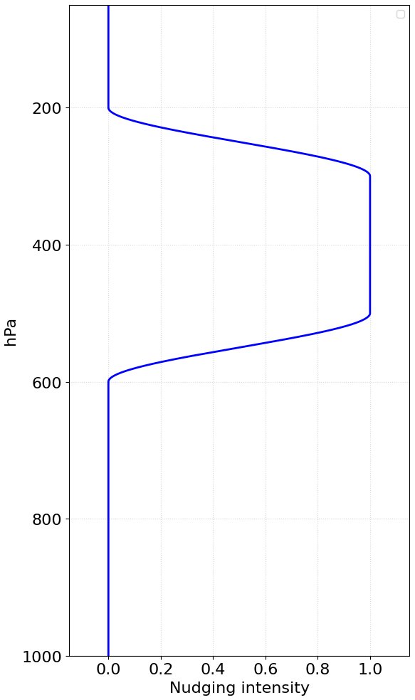
Figure 1 Vertical profile of the nudging intensity (λ_vertical). The horizontal axis represents the intensity, and the vertical axis represents the pressure level (hPa) corresponding to the model level.

To address the issue of sparse vertical resolution of ML model outputs, which limits the accurate representation of three-dimensional large-scale circulations of the lower atmosphere in the model, Husain et al. (2025) adopted a similar vertical coefficient profile. In contrast, Polichtchouk et al. (2024) retrained a 137-model-level version of the AIFS. Notably, Husain et al. (2025) found that the 39-level GraphCast performed worse than the 13-level version, and therefore opted to use the 13-level version in their study. Due to copyright restrictions, We currently do not have access to the training code of FuXi model. In subsequent work, we plan to attempt increasing the number of pressure levels of FuXi, or directly train the FuXi on model levels of CMA-GFS, to see if the hybrid system can be improved in a more comprehensive manner.

(3) Extracting large-scale circulation

The CMA-GFS model employs a 4D-Var data assimilation system (Zhang et al., 2019), in which predictands are first interpolated from latitude–longitude grids to Gaussian grids and subsequently are expanded using spherical harmonic functions (Sardeshmukh and Hoskins, 1984) to facilitate equations solving in spectral space. Since the data assimilation system already contains routines for interpolating between different grids, as well as for spherical harmonic expansion in spectral space, we directly utilize these modules in this study. In contrast, for simplicity of implementation, Husain et al. (2025) applied a discrete cosine transform filter (Denis et al., 2002) directly on the Yin-Yang grid of the GEM model to perform spectral expansion and truncation. Although the discrete cosine transform method is relatively straightforward and generally less accurate than spherical harmonic expansion on Gaussian grids, the present study focuses exclusively on large-scale components. Therefore, the differences between the two methods are negligible and both are considered acceptable for the purposes of large-scale nudging.

A critical aspect of the SN method is the selection of the truncation wavenumber. For instance, in Husain et al. (2025) and Polichtchouk et al. (2024), the truncation wavenumber of 21 was adopted, corresponding to wavelengths greater than approximately 2000 km. In this study, the truncation wavenumber is determined primarily based on the KES differences between the CMA-GFS and FuXi models. Figure 2 illustrates the average KES of the 24 h forecasts from the CMA-GFS and FuXi models for four initial dates: 1 October 2024 and 1 January, 1 April and 1 July 2025. At 850 and 500 hPa, the spectra of FuXi and CMA-GFS forecasts essentially coincide when the wavenumber is lower than 63 (wavelengths larger than ∼700 km), indicating that both models exhibit consistent energy characteristics at these scales. At 100 hPa, the spectra of the two model forecasts remain comparable for wavenumbers smaller than 21 (wavelengths larger than ∼2000 km).

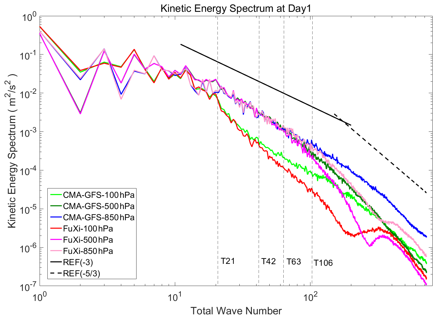
Figure 2 Kinetic energy spectrum (KES) comparison between the China Meteorological Administration Global Forecast System (CMA-GFS, light green: 100 hPa, dark green: 500 hPa, blue: 850 hpa) and FuXi (red: 100 hPa, purple: 500 hPa, pink: 850 hPa) models after the 24 h integration. The horizontal axis represents the spatial scale (wavenumber) of atmospheric motions, and the vertical axis (KES, m² s⁻²) indicates the energy distribution across these scales. Four vertical reference gray dashed lines, T21, T42, T63 and T106, mark the positions corresponding to wavenumbers 21, 42, 63 and 106, respectively.

A primary deficiency of the FuXi model manifests at meso- and small scales, where kinetic energy decays rapidly. This reflects a common limitation of current ML models, in which forecast fields become increasingly smooth with lead time, leading to inadequate representation of meso- and small-scale weather systems. The slight increase of kinetic energy in the FuXi model at smaller scales is attributed to computational noise, characterized by widespread sawtooth-like fluctuations. The distribution of the vertical nudging coefficient (Fig. 1) indicates that the effective vertical range of nudging is primarily between 600 and 200 hPa. Thus, we initially select a truncation wavenumber of 42 (corresponding to a wavelength of approximately 1000 km) in this study.

However, we find that the 500 hPa KES from the hybrid system shows distinct characteristics across different forecast leading times (5 and 10 d) in a typical case (Fig. 3). At day 5, the KES from the hybrid system essentially coincides with that from the CMA-GFS for all truncation wavenumbers (T21, T31 and T42). By day 10, the KES under the T21 configuration exhibits slight attenuation in the wavenumbers of 20–30, while the KES under the T31 and T42 shows attenuation in the wavenumber ranges of 20–40 and 20–60, respectively. Such attenuation causes synoptic-scale waves to become smoother at longer forecast leading times, reflecting some characteristics of ML models. We compared several different dates, including the 4 d in Fig. 2. Across these cases, the 500 hPa KES show no decay on day-5, while varying magnitudes of KES decay emerge by day-10. To better illustrate this feature, we chose the case exhibiting the strongest decay, instead of showing multi-sample averaged KES as in Fig. 2.

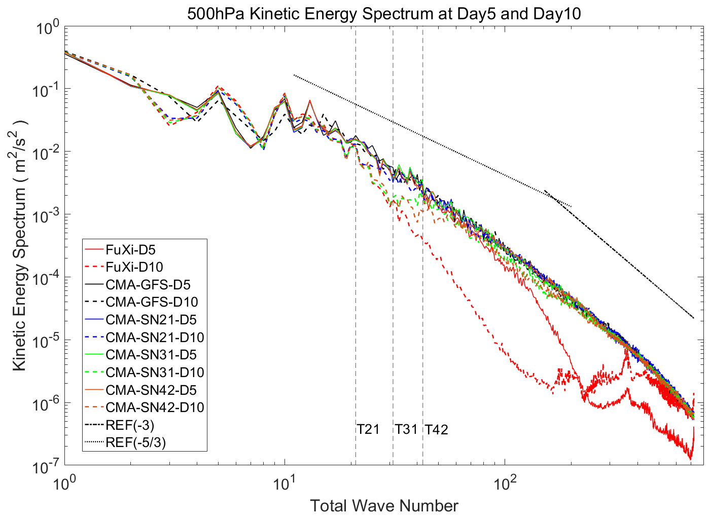
Figure 3 Comparison of the 500 hPa KES of 5 d (solid lines) and 10 d (dashed lines) forecasts for a typical case on 1 July 2024. Black and red lines represent the KES of the CMA-GFS and FuXi forecasts, respectively, and blue, green and brown lines denote the KES from the CMA-SN with truncation wavenumbers of 21, 31, and 42, respectively. Three vertical reference gray dashed lines, T21, T31 and T42, denote the positions corresponding to wavenumbers 21, 31 and 42, respectively.

To further assess the impact of different truncation wavenumbers on model forecast performance, we compare the characteristics of the hybrid system forecasts under the T21 (hereafter referred to as CMA-SN21) and T42 (hereafter referred to as CMA-SN42) configurations through case studies (Fig. 4) and batch experiments (Figs. 5–10). Given that T42 does not deliver superior forecast performance relative to T21, we adopted the T21 to prevent mesoscale circulations in the hybrid system from becoming excessively smoothed by AI-model influences at later forecast lead times (around day 10).

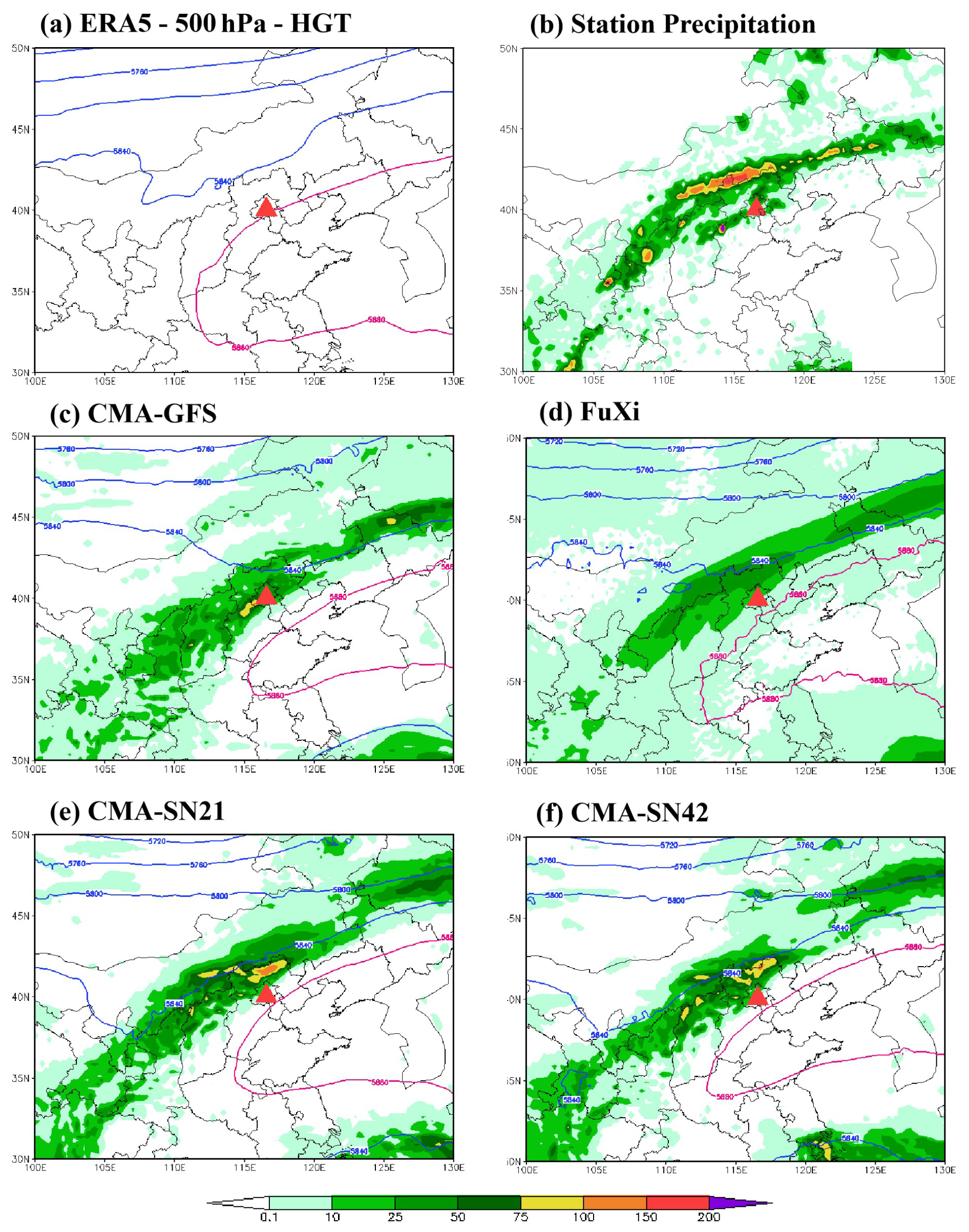
Figure 4 Comparison of the 500 hPa geopotential height and the 24 h accumulated precipitation for a heavy rainfall case in North China: (a) 500 hPa geopotential height from the ERA5 data, (b) Station-observed precipitation, and forecasts from the (c) CMA-GFS, (d) FuXi, (e) CMA-SN21 and (f) CMA-SN42. Contours represent the geopotential height (unit: gpm), and shading indicates rainfall amount (unit: mm). The red triangle marks the location of Beijing Municipality.

2.3.1 (4) Incorporating the correction term into the dynamic core of the CMA-GFS

The correction term $-\mathit{\lambda }(\mathit{\psi }-{\mathit{\psi }}_{\mathrm{ref}}{)}_{\mathrm{LS}}$ is incorporated into the nonlinear terms during the linearization process of the semi-implicit algorithm and participates in the solution process of the dynamic core of the CMA-GFS model. In the initial implementation, nudging is applied only to the variables of π and θ, and it is further extended to u and v, which can improve the forecast skill for wind fields, especially in tropical regions. Note that nudging is not applied to humidity variables, because that nudging is already applied to wind fields, so the distribution of passive scalars can be subsequently adjusted through advection processes. Additionally, incorporating the large number of moisture variables would substantially increase computational demands if included in the nudging procedure.

Table 2 presents a comparison of the differences in technical details of the SN method among ECCC (Husain et al., 2025), ECMWF (Polichtchouk et al., 2024, 2026), and CMA (our work).

Table 2 The differences in technical details of the SN method.

Table 3 Experiment setup.

3 Evaluation of the online correction system

3.1 Experiment setup

Four sets of experiments are conducted (Table 3). Since the FuXi model was trained using the ERA5 reanalysis dataset, it performs best when using the ERA5 data as initial conditions, while using the CMA-GFS 4D-Var analysis data as the initial conditions may degrade model performance. For instance, the lead time for the forecasts in July 2024 decreases by 0.7 d in the Northern Hemisphere and by 2.0 d in the Southern Hemisphere compared with using the ERA5 as initial conditions. This is commonplace in ML models, and the methods for addressing it within the final 4D-Var system will be discussed in the conclusion section. Given that the primary aim of this work is to demonstrate the feasibility of the concept, and the establishment of the entire 4D-Var system is not yet complete, all experiments and systems in this study use the ERA5 data as initial conditions.

3.2 Case study

We first conduct simulations of a representative high-impact weather event to provide a direct comparison of the forecast characteristics of the CMA-GFS, FuXi, CMA-SN21 and CMA-SN42. The selected case is a heavy rainfall event that occurred over central Inner Mongolia, North China, on 25 and 26 July 2025. During this event, the western Pacific subtropical high (WPSH) was anomalously strong, with its ridge extending westward and northward while maintaining stability. Under the influence of cold air intrusions from the westerlies, the convergence of cold and warm airflows, together with long-range moisture transport from the peripheral circulation of a typhoon over the eastern seas of China, resulted in persistent and intense precipitation on the northern flank of the WPSH.

Due to the fixed resolution of the FuXi model, the other three experiments also adopt the horizontal resolution of 0.25° to ensure comparability. Forecast integrations are initialized at 12:00 UTC on 20 July 2025 and run for 10 d. The 500 hPa geopotential height after the 120 h integration and the 24 h accumulated rainfall amount after the integration of 108–132 h are compared.

At 12:00 UTC on 25 July, the WPSH (represented by the 5880 gpm contour at 500 hPa) extended westward to 112° E, with its northern boundary passing through the southern part of Beijing (Fig. 4a), significantly westward and northward of climatology. The precipitation center on the northern side of the WPSH was located to the northwest of Beijing, with the 24 h accumulated precipitation reaching 100–200 mm (Fig. 4b). In the CMA-GFS simulation (Fig. 4c), the western ridge of the WPSH lies near 115° E, and its northern edge is approximately 2° latitude south of Beijing. The simulated WPSH is weaker and displaced farther eastward and southward relative to observations. Its precipitation center was west of Beijing, with maximum 24 h rainfall of 50–75 mm. FuXi simulation (Fig. 4d) had a WPSH position consistent with ERA5 (Fig. 4a) and a precipitation center roughly matching observations, but with notably weaker intensity (<50 mm) and overly smooth distribution. CMA-SN21 and CMA-SN42 (Fig. 4e and f) had WPSH positions close to FuXi. Their rain band location was more consistent with observations than CMA-GFS, with maximum precipitation of 100–150 mm, showing obvious improvement over both FuXi and CMA-GFS. With the improved circulation patterns, the wind, pressure, temperature and humidity fields achieve better mutual consistency. Driven by the model's internal physical parameterizations, the simulated precipitation intensity is more realistic and agrees better with observations. The results confirm that the hybrid system effectively combines the superior forecasting skill of ML models for large-scale circulations with the strengths of physical models in simulating precipitation intensity and fine-scale structures, consistent with the expectations of this study.

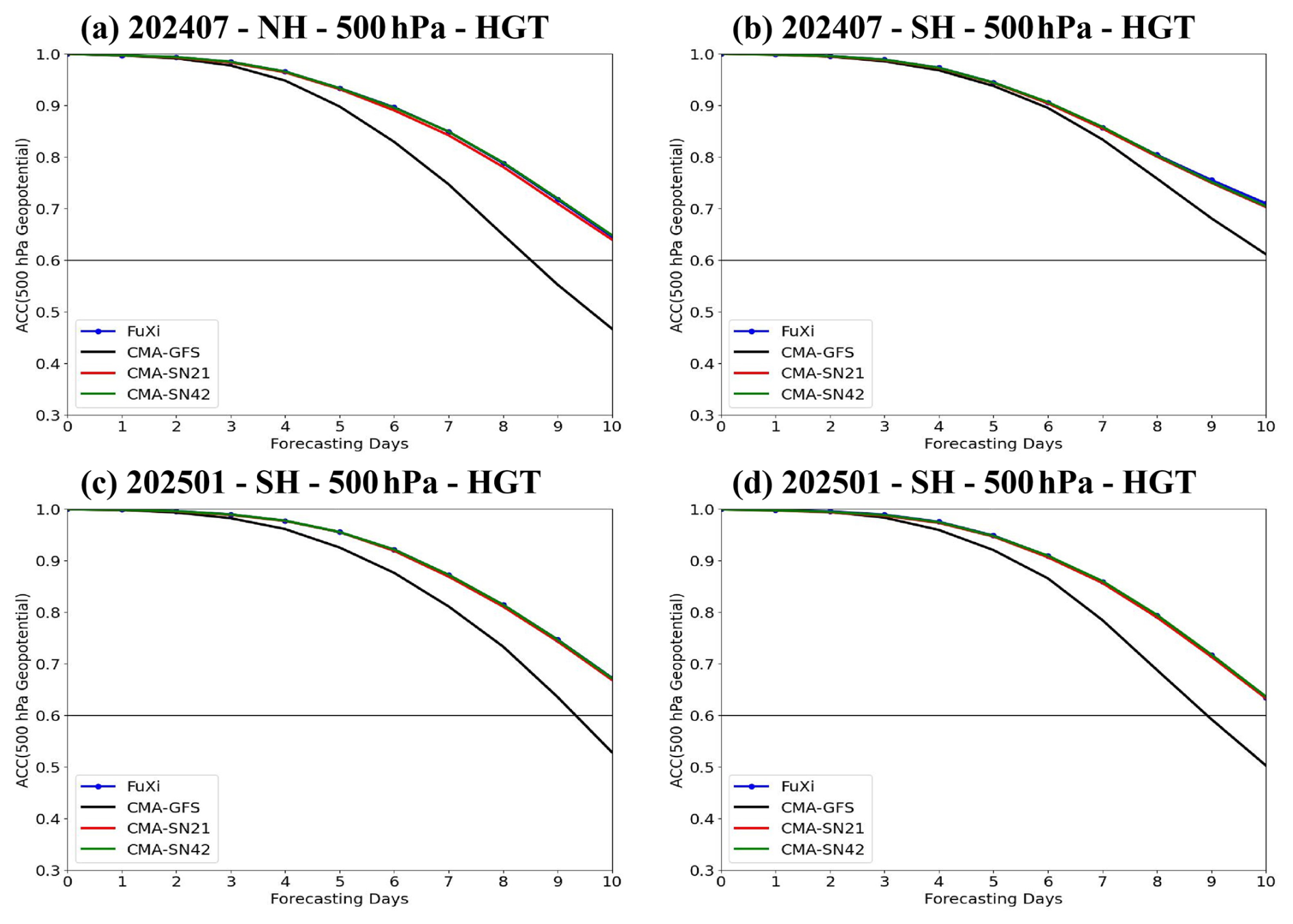
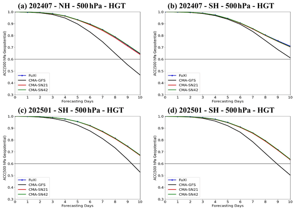
Figure 5 ACC of the 500 hPa geopotential height forecasts in (a, c) the Northern Hemisphere (NH) and (b, d) Southern Hemisphere (SH) for (a, b) July 2024 and (c, d) January 2025 from the FuXi (blue lines with dots), CMA-GFS (black lines), CMA-SN21 (red lines) and CMA-SN42 (green lines).

3.3 Evaluation based on batch experiments

Batch experiments are conducted for July 2024 and January 2025, which is initiated daily at 12:00 UTC and integrated for 10 d. The horizontal resolution of the CMA-GFS and CMA-SN is set to 0.125°, consistent with that of the operational CMA-GFS model. Due to inherent constraints, the FuXi model is run at its native resolution of 0.25°.

Figure 5 presents the ACC of 500 hPa geopotential height forecasts for July 2024 and January 2025 from FuXi, CMA-GFS, CMA-SN21 and CMA-SN42. Using ERA5 as initial conditions, CMA-GFS had a forecast lead time of ∼8.5 d (Northern Hemisphere) and 10 d (Southern Hemisphere) in July 2024, and ∼9.3 d (Northern Hemisphere) and 8.8 d (Southern Hemisphere) in January 2025. FuXi showed obvious advantages in large-scale circulation simulations, with its lead time exceeding CMA-GFS by ∼2 d in July and ∼1.5 d in January. The hybrid system essentially inherited FuXi's 500 hPa large-scale circulation characteristics, as CMA-SN21 and CMA-SN42 ACC values were largely consistent with FuXi's throughout the forecast period – consistent with the method design, determined by the nudging algorithm's temporal and vertical coefficients. The differences between CMA-SN21 and CMA-SN42 were negligible, so only CMA-SN21 forecasts were used for subsequent evaluations.

The ACC of 500 hPa geopotential height forecasts on day 5 of the integration indicates forecast skill stability. Figure 6 shows the ACC values of CMA-GFS and CMA-SN21 over the Northern Hemisphere in July 2024 and January 2025. The ACC scores of the CMA-GFS drop substantially on 17 July, 10, 14, and 23 January, indicating considerable errors in the large-scale circulation. This phenomenon is likely associated with extreme weather events such as typhoons and cold waves. Such instability in forecast skill can substantially undermine forecaster confidence in model outputs. The hybrid system developed in this study markedly alleviates this issue. Throughout the batch experiments, its forecast skill remained within a relatively narrow, reasonable variability range, reflecting marked improvement in model forecast reliability.

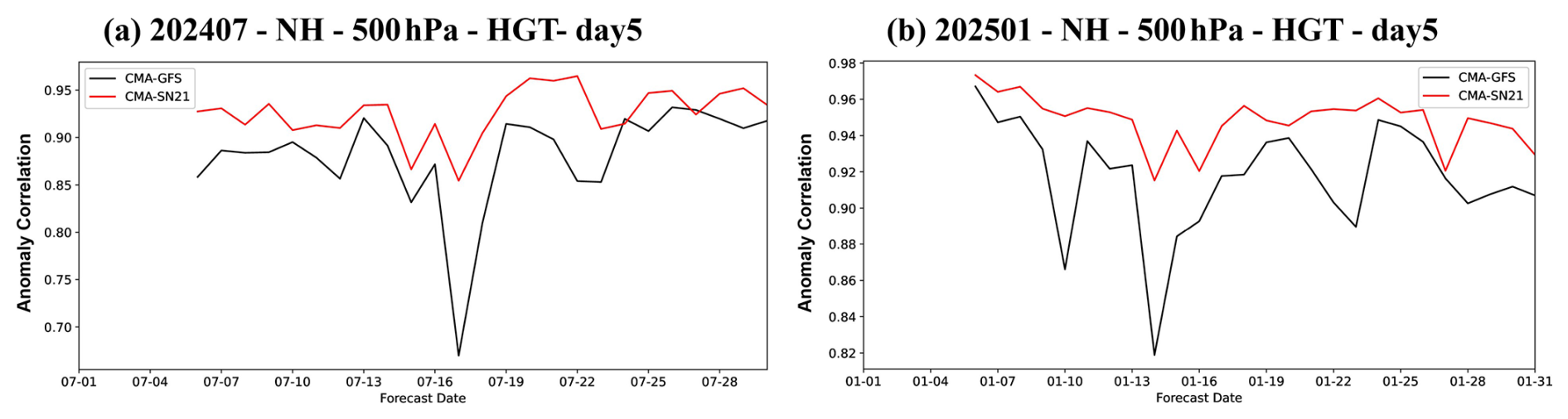
Figure 6 ACC of the 500 hPa geopotential height forecasts from CMA-GFS (black lines) and CMA-SN21 (red lines) experiments on day 5 of the integration over the NH in (a) July 2024 and (b) January 2025.

Figure 7 illustrates the vertical extent of the improvements after introducing the SN algorithm. In the geopotential height forecasts, the CMA-SN model demonstrates marked improvement from 925 to 10 hPa. However, negative contributions exist above 10 hPa, the reasons for which require further analysis. In terms of the temperature forecasts, the improvement from the CMA-SN model extends up to approximately 5 hPa in summer and is primarily confined below 100 hPa in winter. For tropical wind fields, the CMA-SN achieves a notable reduction in the RMSEs during both summer and winter, primarily between 850 and 50 hPa.

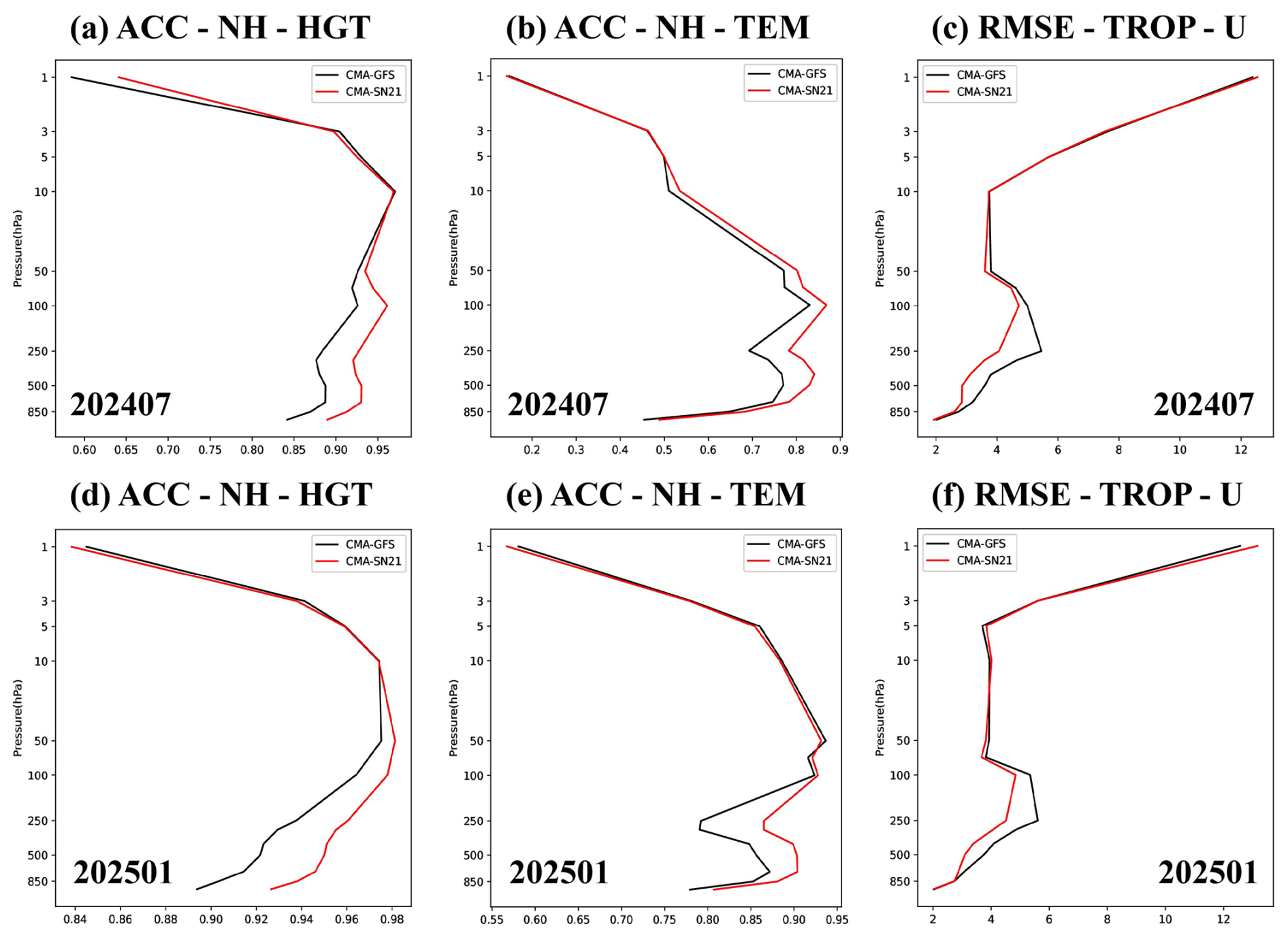
Figure 7 (a, b, d, e) Vertical profiles of the ACC values of (a, d) geopotential height and (b, e) temperature forecasts and (c, f) vertical profiles of RMSE of wind speed forecasts (unit: m s⁻¹) from experiments CMA-GFS (black lines) and CMA-SN21 (red lines) on day 5 of the integration over the NH in (a–c) July 2024 and (d–f) January 2025.

Moreover, the zonally averaged vertical distributions of simulated geopotential height biases from CMA-GFS, CMA-SN21 and FuXi are discussed (Fig. 8). The CMA-GFS shows distinct negative biases in the middle and upper levels, particularly large in polar regions. The FuXi exhibits a similar overall spatial distribution to CMA-GFS but with notably smaller biases. The CMA-SN21's bias distribution is not a simple combination of the two parent models: above 500 hPa, its bias pattern closely resembles FuXi's but with slightly smaller magnitudes; below 500 hPa, its errors are distributed similarly to CMA-GFS, but with generally larger negative values except for winter Northern Hemisphere high latitudes (slightly larger positive biases).

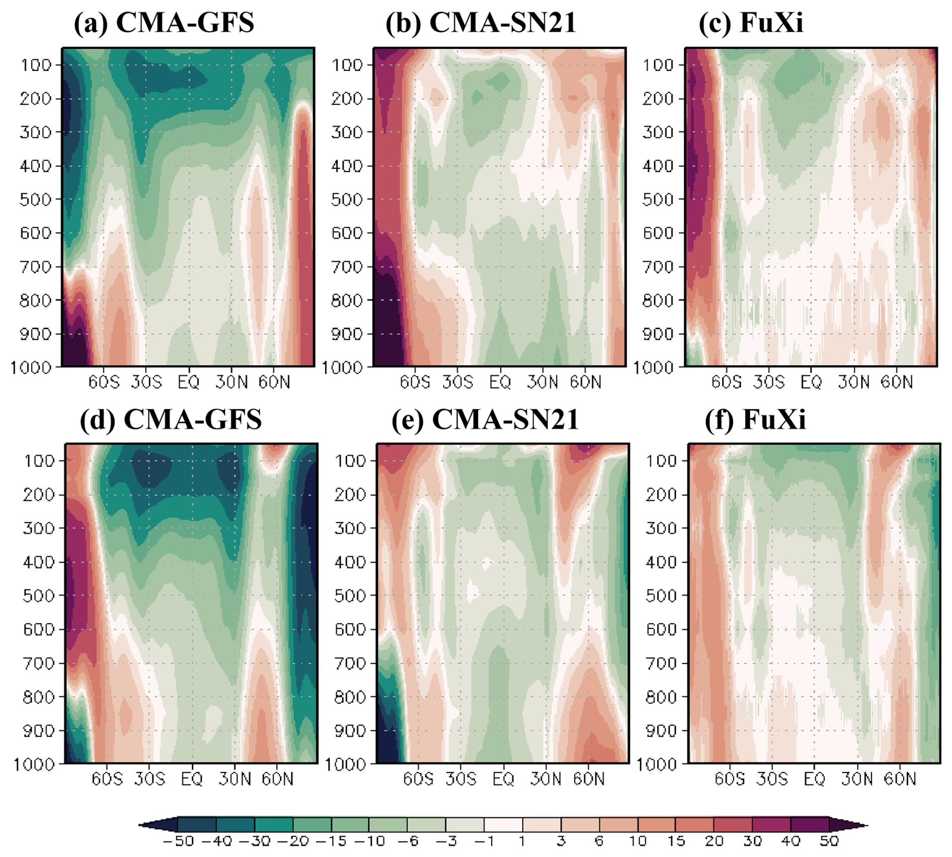
Figure 8 Zonally averaged vertical profiles of geopotential height biases (unit: gpm) for 7 d forecasts relative to ERA5 analysis, from (a, d) CMA-GFS, (b, e) CMA-SN21, and (c, f) FuXi, in (a–c) July 2024 and (d–f) January 2025.

The zonally averaged vertical distribution of the biases of temperature simulations (Fig. 9) resembles that of the geopotential height simulations. The CMA-GFS temperature simulations are characterized by predominantly negative biases in the middle and upper levels and positive biases in the lower levels and near 100 hPa. The FuXi simulations exhibit positive biases in the lower levels and predominantly negative biases in the upper levels, with bias magnitudes substantially smaller than those of the CMA-GFS simulations. The CMA-SN21 temperature bias distribution is largely consistent with CMA-GFS in the lower levels. In the middle and upper levels, the CMA-SN incorporates forecast features from both the CMA-GFS and FuXi, effectively eliminating the obvious negative temperature biases of CMA-GFS above 500 hPa.

Figure 9 Same as Fig. 8, but for temperature biases (unit: °C).

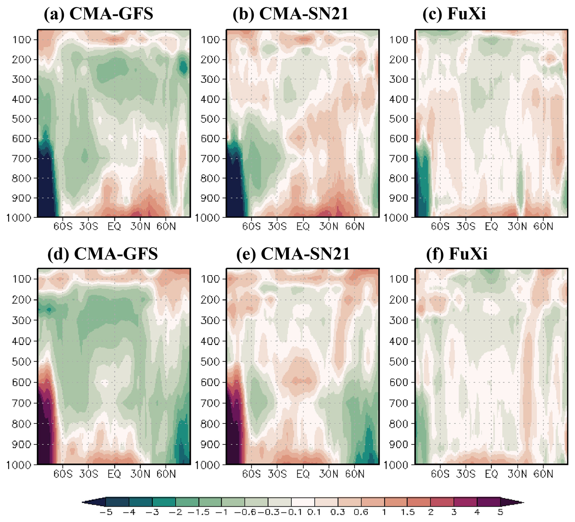
The vertical distributions of the temperature and geopotential height biases reveal that the CMA-SN bias structure is highly correlated with the vertical coefficients of the nudging intensity shown in Fig. 1. Therefore, the forecasts at lower model levels are predominantly influenced by the dynamical and physical processes within the CMA-GFS. However, forced by more accurate middle and upper level large-scale circulations, lower level meso- and small-scale system position forecasts are improved. For the upper levels, although the nudging coefficient extends only to 200 hPa, changes in the upper-tropospheric circulations can influence stratospheric forecasts through the action of large-scale circulations such as the Hadley and Ferrel cells, thereby reducing stratospheric forecast errors.

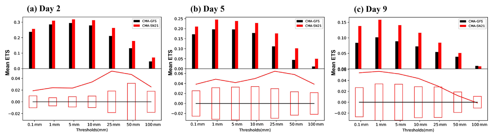
Figure 10 Equitable threat scores (ETSs) of the 24 h accumulated precipitation simulations from the CMA-GFS (black bars) and CMA-SN21 (red bars) on (a) day 2, (b) day 5, and (c) day 9 of the integration over China in July 2024. The red lines represent the difference in the ETSs between the CMA-SN21 and CMA-GFS, and the red boxes indicate the 0.05 significance level. If the red lines extend outside the red boxes, they indicate that the difference passes the 0.05 significance test.

As the forecast leading time increases, the improvement from online large-scale circulation correction becomes more pronounced. Even without any modification to physical parameterization schemes, precipitation forecasts show substantial improvement under the influence of more accurate large-scale circulations. The Equitable Threat Score (ETS), a categorical verification index for precipitation, is used to assess forecast skill at different precipitation thresholds. It accounts for random correct forecasts, with values ranging from $-\mathrm{1}/\mathrm{3}$ to 1. Larger ETS values indicate better agreement between forecast and observed precipitation. The precipitation observation dataset used for ETS scores is the China national-station 6 h precipitation dataset (∼2515 stations), which has a temporal resolution of 6 h (24 h accumulated precipitation is also supported) and consists of discrete station observations. For model-observation matching, model grided forecasts are bi-linearly interpolated to station geographic coordinates, forecast accumulation windows are temporally aligned with station observations, and point-to-point pairs are adopted to build contingency tables for ETS computation. The ETS statistical domain covers Chinese mainland within 73–136° E, 18–54° N, and the significance test is implemented via non-parametric bootstrap resampling to obtain the 95 % confidence interval (α=0.05) for ETS scores. Figure 10 indicate that the CMA-SN exhibits a notable improvement in the ETSs across all precipitation thresholds, and this enhancement increases with forecast leading time. Although the ETS on day 9 is not typically the focus of verification, it nevertheless provides a meaningful indication of the enhancement in the precipitation forecast capability of the hybrid system.

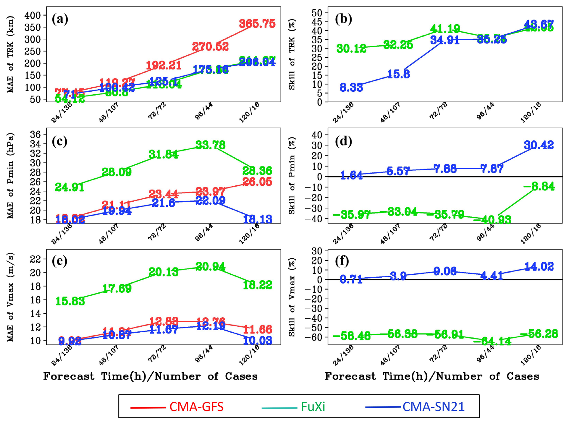
Figure 11 Evaluation of the model forecasting performance using 10 typhoon cases with lifespans greater than 5 d over the western North Pacific and the South China Sea in 2024: (left axes) mean absolute errors (MAEs) and (right axes) percentage improvement of the forecasts of the (a, b) typhoon tracks (TRK; unit: km), (c, d) central pressure (Pmin; unit: hPa) and (e, f) maximum wind speed (Vmax; unit: m s⁻¹) from the FuXi and CMA-SN21 relative to the CMA-GFS forecasts. x axis: forecast lead time/number of valid samples.

3.4 Evaluation based on typhoon forecasts

The performance of the CMA-SN21 is further examined through typhoon simulation experiments. The sample set consists of 10 typhoon cases with lifespans exceeding 5 d over the western North Pacific and the South China Sea in 2024: Gaemi (No. 2403), Shanshan (No. 2410), Yagi (No. 2411), Bebinca (No. 2413), Pulasan (No. 2414), Krathon (No. 2418), Kong-Rey (No. 2421), Yinxing (No. 2422), Toraji (No. 2423) and Man-yi (No. 2424). Three experiments are conducted using CMA-GFS, FuXi and CMA-SN21, all initialized with ERA5 data and performed at a uniform 0.25° horizontal resolution. The best-track dataset is sourced from the Shanghai Typhoon Institute (STI) of CMA (https://tcdata.typhoon.org.cn/, last access: 23 January 2026). TC center positions are determined using a two-step algorithm. First, first-guess estimation uses the TC position from the prior time step as the starting point. The search radius is computed from the maximum plausible TC translation speed (∼150 km h⁻¹) multiplied by the model output time interval. The location of minimum 1.5 km altitude pressure perturbation within this domain yields the first-guess center. Second, vorticity centroid refinement calculates the 1.5 km altitude vorticity centroid by spatially weighting relative vorticity within a 300 km radius of the first-guess position. Representing the TC's rotational dynamical core, the vorticity centroid refines center localization and reduces biases induced by small-scale perturbations.

Figure 11a–f presents the mean absolute errors (MAEs) and percentage improvement of the typhoon track, central pressure and maximum wind speed forecasts from the FuXi and CMA-SN21 relative to the CMA-GFS forecasts. CMA-GFS has larger typhoon track errors, with an MAE of ∼365 km on integration day 5, while FuXi track forecasts are much more accurate (MAE of 206 km on day 5). CMA-SN21 track errors are essentially comparable to FuXi's, with an effective improvement of ∼30 %–40 % relative to CMA-GFS. ML models commonly suffer from an over-smoothing tendency with increasing forecast leading time, a deficiency that is particularly evident in typhoon intensity forecasts. FuXi systematically underestimates typhoon intensities, with MAEs of ∼30 hPa for central pressure and 15–20 m s⁻¹ for maximum wind speed. In contrast, the typhoon intensities simulated by the CMA-GFS are closer to the observations, with MAE values of around 20 hPa for central pressure and 10 m s⁻¹ for maximum wind speed. CMA-SN21's typhoon intensity performance is similar to CMA-GFS, and even outperforms it at longer lead times. This improvement indicates that the enhanced circulation yields better consistency among wind, pressure, temperature and moisture fields, allowing the physical mechanisms within the numerical model to produce more realistic tropical cyclone evolution.

4 Conclusions and discussion

The in-depth integration of novel ML models with conventional physical models represents an inevitable direction for the future development of earth system modeling. Major operational forecasting centers worldwide have formulated differentiated model-fusion strategies and roadmaps based on their respective technological strengths, development stages and application scenarios. In this study, we independently implement an online correction system based on the SN method using a distinct combination of physical and ML models compared with Husain et al. (2025) and Polichtchouk et al. (2024, 2026), and further validate the concept that this hybrid system can fully leverage ML-model strengths in large-scale circulation forecasting to boost the forecast skill of conventional physical NWP models. The main conclusions of this research are as follows.

This study demonstrates that the KES of the CMA-SN simulations remains consistent with that of the CMA-GFS simulations across all wavelength ranges, thereby achieving the intended research objective. The CMA-SN effectively enhances the forecasting skill for large-scale circulations while retaining the inherent characteristics of the CMA-GFS in capturing meso- and small-scale systems, thereby ensuring detailed representation and the capability to predict extreme weather events. With more accurate large-scale circulations, the physical mechanisms represented in the CMA-GFS can further improve the simulations of the initiation and evolution of high-impact weather phenomena, such as heavy rainfall and typhoons.

The present research suggests that if ML models cannot fully overcome key challenges – such as over-smoothing and limited short-range extreme-event prediction – constructing an online correction system based on the SN method provides a feasible technical pathway. This approach offers a promising alternative for the global medium-range NWP.

The future development of the online correction system involves several key considerations:

1. In this proof-of-concept study, both CMA-GFS and FuXi are initialized with ERA5 data. This setup cannot fully represent the performance of a real-time operational system. The next step is to establish a cycling 4D-Var system within the online correction framework, ultimately aiming to enhance CMA operational global medium-range forecasts. Building this cycling system first requires developing the workflow, modifying the CMA-GFS 4D-Var system (including its tangent linear and adjoint models) and adjusting the background error covariance. Subsequently, A critical challenge that must be overcome is the degradation in forecasting skill when using the CMA-GFS analysis data as the initial conditions of the FuXi model – a common problem in ML models. Two approaches are currently employed to address this. The one involves employing Transformer-based neural network models to adjust the CMA-GFS analysis fields, rendering them more consistent with the ERA5 reanalysis data, before applying them to the FuXi model. The other approach involves fine-tuning or retraining the FuXi model using CMA reanalysis data derived by the CMA-GFS system and CMA-GFS analysis fields to improve the adaptability of the FuXi model.

2. The interface of the ML model is designed to be generic. As long as the outputs of ML models are provided on standard pressure levels, the CMA-SN system can accommodate outputs with different vertical resolutions and temporal frequencies. Future work will follow advancements in ML models to potentially expand the vertical coverage and temporal frequency of nudging, thereby further improving forecast skill.

3. The flexibility of the interface also enables the hybrid system to switch seamlessly between different ML models. In this study, the FuXi model is selected due to its superior forecasting performance. In the future, a transition to the FengQing model, an ML model independently developed by the CMA, is under consideration. This transition would support the goal of establishing a fully self-developed forecasting chain.

4. Ensemble forecasting can quantify forecast uncertainty, provide information such as probabilistic forecasting, and has been widely applied in practical operations. Future work may establish an ensemble forecasting system integrating physical models and ML models based on the SN method. ECMWF provides a valuable benchmark (Polichtchouk et al., 2026) for establishing the SN ensemble forecast system. Since we have already established the workflow for the deterministic SN system, the key to extending it to ensemble forecasting is to maintain reasonable spread among ensemble members. For example, we need to perform SN between the 16 corresponding members of CMA-GEPS (Global Ensemble Prediction System) and FuXi-ENS, rather than nudging all CMA-GEPS members toward a single FuXi deterministic forecast. In addition, how to specify model perturbation also requires discussion and testing.