SeapoPym v0.1: implementation of the SEAPODYM low and mid trophic levels in Python with a flexible optimization framework

SEAPODYM-LMTL, the low and mid trophic level component of SEAPODYM, simulates mesozooplankton and micronekton biomass globally as an advection-diffusion-reaction system driven by physical and biogeochemical forcing. Its mesozooplankton parameterization remains incompletely calibrated, and its operational implementation couples the biological equations to spatial transport, so evaluating a parameter set requires running the full spatial model, which makes automated calibration costly. We present SeapoPym v0.1, an open-source Python re-implementation of the SEAPODYM-LMTL biological model that solves the dynamics locally, without transport. We apply it to the single epipelagic mesozooplankton group and estimate its five biological parameters with a covariance matrix adaptation evolution strategy (CMA-ES). Comparison with the operational product shows that omitting transport matters most in strongly advective regions and in cold high-latitude waters, where the long zooplankton life cycle keeps the biomass exposed to advection. At six contrasting stations the difference between the two models stays between 6 % and 12 % of the simulated biomass, five to seven times smaller than the model-observation gap where in-situ records allow that comparison. A Sobol analysis attributes the magnitude of the biomass to the energy-transfer and mortality parameters, and the timing of the seasonal peak to the recruitment parameters. Twin experiments then show that parameter identifiability depends on the environmental regime sampled. Wherever the search converged, energy transfer and mortality were recovered, whereas recruitment was recovered only in cold water. A single cold station constrained all five parameters as well as the six stations combined, so recovery follows the information content of the sampled regime rather than the number of stations. These results hold for noise-free synthetic observations generated by the transport-free model itself and driven by the exact forcing. The next step is to repeat them under realistic sampling and forcing error, then calibrate the model against in-situ records.

1 Introduction

Mesozooplankton connect primary production to higher trophic levels and contribute to ocean carbon export. They are conventionally defined as planktonic organisms ranging from 0.2 to 20 mm (Sieburth et al., 1978), dominated by copepods, although the size class is taxonomically diverse (Moriarty and O'Brien, 2013; Drago et al., 2022). They provide a major food source for micronekton (2–20 cm), including mesopelagic fish, euphausiids and gelatinous organisms (Brodeur et al., 2005; St. John et al., 2016). Mesozooplankton also contribute to the transformation and export of organic matter (Steinberg et al., 2000, 2002; Stukel et al., 2022; Siegel et al., 2023). Changes in their biomass or seasonal timing can therefore affect both prey availability and carbon export, making their representation a leading source of uncertainty in global biogeochemical models (Rohr et al., 2023).

The SEAPODYM-LMTL model provides operational global simulations of mesozooplankton and micronekton biomass. It is the Low and Mid-Trophic Levels (LMTL) component of SEAPODYM, a model developed to simulate tuna and tuna-like populations (Lehodey et al., 2008). SEAPODYM-LMTL represents their prey environment through one mesozooplankton and six micronekton functional groups (Lehodey et al., 2010; Conchon, 2016). It couples biological processes with advection and diffusion and is driven by currents, temperature, euphotic depth and net primary production (NPP). The resulting biomass fields are distributed through the Copernicus Marine Service for ecosystem and fisheries applications (Titaud et al., 2024).

The mesozooplankton parameterization of the SEAPODYM-LMTL model remains incompletely calibrated, and its operational product shows substantial differences from observations. Of its five biological parameters, only the energy-transfer coefficient has been formally calibrated against mesozooplankton observations. The four parameters controlling the temperature dependence of recruitment and mortality are derived from the literature or manual tuning (Huntley and Lopez, 1992; Gillooly, 2000; Gillooly et al., 2002; Conchon, 2016; Titaud et al., 2024). When compared to in-situ observations (direct mesozooplankton biomass measurements) from the COPEPOD database (O'Brien, 2014), the operational SEAPODYM-LMTL product yields a coefficient of determination of R²=0.11, while its global mean biomass is 1.19 g C m⁻², compared with 0.76 g C m⁻² in the observations (Titaud et al., 2024). These differences motivate a systematic recalibration of the biological component.

The operational SEAPODYM-LMTL implementation does not provide a practical route for automated parameter calibration. Its biological equations are embedded in a non-public C$++$ code and tightly coupled to the spatial transport component through an implicit solver. Evaluating each parameter set would therefore require running the full spatial model, whereas an optimization typically requires thousands of such evaluations. This makes systematic calibration computationally impractical at global scale or at fine resolution, and prevents the biological component from being tested independently.

An open and lightweight implementation that separates the biological equations from spatial transport and can be coupled directly to optimization algorithms is therefore needed. For this, we developed SeapoPym, an open-source Python re-implementation of the SEAPODYM-LMTL biological model, together with a flexible framework for automated parameter optimization. SeapoPym isolates the biological equations from spatial transport and solves the temperature- and NPP-driven dynamics locally in a zero-dimensional configuration, allowing many parameter sets to be evaluated efficiently. Two experiments establish whether SeapoPym is a valid basis for parameter optimization. We verify that it converges to the analytical steady state of the reference equations, and we quantify how far it departs from the operational SEAPODYM-LMTL product.

Two further experiments, under controlled conditions, establish whether the five biological parameters can be recovered, and from which observations. The first, a Sobol sensitivity analysis, determines what each parameter controls, the magnitude of the biomass or the timing of its seasonal peak. The second, a set of twin experiments, measures identifiability, the capacity to recover the true parameter values from the data. The optimization framework must recover known parameter values from synthetic biomass time series the model generated itself, across contrasting environmental regimes from cold and productive to warm and oligotrophic. These experiments are a prerequisite to any real-data calibration.

All abbreviations used in this paper are listed in Appendix C.

2 Material and methods

2.1 SEAPODYM-LMTL (the reference model)

SEAPODYM (Spatial Ecosystem and Populations Dynamics Model) was originally developed to simulate the dynamics of tuna and tuna-like populations under the combined influence of fishing and the environment (Lehodey et al., 2008). Its lower trophic levels are represented by a dedicated component, SEAPODYM-LMTL (Low and Mid-Trophic Levels), which the SeapoPym model re-implements and which we describe here. In its first versions, SEAPODYM-LMTL represented the lower trophic levels as a single biomass pool, the prey (“forage”) available to tuna (Lehodey et al., 1998; Lehodey, 2001). That pool was later split into one mesozooplankton group and six micronekton groups (Lehodey et al., 2010; Conchon, 2016). It simulates their biomass as a system of advection-diffusion-reaction equations driven by physical and biogeochemical forcing (Lehodey et al., 2010). Its operational hindcast is distributed through the Copernicus Marine Service (product GLOBAL_MULTIYEAR_BGC_001_033) as a set of Essential Ocean Variables for downstream ecosystem and fisheries applications (E.U. Copernicus Marine Service Information, 2024; Titaud et al., 2024). The operational implementation is written in C++, with the biological reaction terms tightly coupled to both advection and diffusion terms within the numerical solver.

SEAPODYM-LMTL represents the pelagic habitat with three vertical layers whose boundaries follow the euphotic depth Z_eu: an epipelagic layer (down to 1.5 Z_eu), an upper mesopelagic layer (to 4.5 Z_eu), and a lower mesopelagic layer (to 10.5 Z_eu, capped at 1000 m) (Lehodey et al., 2010, 2015). The six micronekton groups are defined by their diel vertical migration between these layers: three stay in a single layer over the day-night cycle, and three migrate, tracking the light field (Lehodey et al., 2010). For the migrating groups, the temperature and currents they experience are averaged over the layers they occupy by day and by night, weighted by day length (Lehodey et al., 2010). Mesozooplankton, which are the focus of this study, are represented by a single group which inhabits the epipelagic layer, does not migrate (Conchon, 2016), and is independent of other groups (see also Appendix A). Diel vertical migration therefore does not apply to it, and the vertical structure reduces to the epipelagic layer alone.

The biology of the mesozooplankton group rests on three coupled processes: energy intake from primary production, aging through an age-structured zooplankton production (p), and its recruitment (R) into a zooplankton biomass (B) pool that is subject to mortality. A fixed fraction E of NPP enters the youngest production class, and this production ages as a daily cohort until it is recruited into the biomass pool at a temperature-dependent recruitment age τ_r (Lehodey et al., 2010; Conchon, 2016). The biomass pool then declines through a temperature-dependent mortality rate λ, so that at steady state the biomass equals the recruitment flux divided by the mortality rate, $B_{\mathrm{eq}}=R/\mathit{\lambda }$ (Lehodey, 2001). The recruitment age and the mortality timescale $\mathrm{1}/\mathit{\lambda }$ both shorten with temperature, following the exponential form expressed in the normalized temperature $\stackrel{\mathrm{‾}}{T}=T/(\mathrm{1}+T/\mathrm{273})$ (Lehodey et al., 2010), after the metabolic theory of Gillooly (2000); Gillooly et al. (2002). Production ages by one class per day and the model resolves at most eleven daily cohorts, set by the maximum recruitment age (${\mathit{\tau }}_{{\mathrm{r}}_{\mathrm{0}}}=\mathrm{10.38}$ d, reached at the reference temperature T_ref=0 °C). The full equations and their numerical solution are given in Appendix A. The spatial transport that SeapoPym omits, an advection-diffusion scheme shared with the upper-trophic-level model, is described in Sibert et al. (1999) and Lehodey et al. (2008).

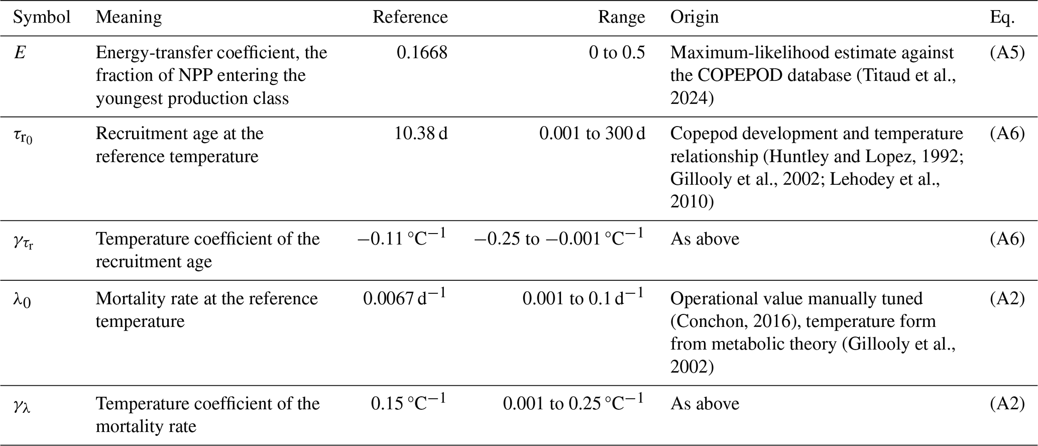
The reference values of the five biological parameters are listed in Table 1. The recruitment and mortality temperature relationships are taken from the literature on copepod development and metabolism (Huntley and Lopez, 1992; Gillooly, 2000; Gillooly et al., 2002), whereas the energy-transfer coefficient was estimated by maximum likelihood against the COPEPOD mesozooplankton database, where it reaches E≈0.167, above the canonical 10 % trophic-transfer efficiency (Titaud et al., 2024). These values have been refined across successive versions of the operational SEAPODYM-LMTL product, but the five parameters have never been estimated jointly: the micronekton energy-transfer coefficients were optimized separately against acoustic data (Lehodey et al., 2015) and in a synthetic observing-system experiment (Delpech et al., 2020), while the zooplankton recruitment and mortality parameters were manually tuned (Conchon, 2016).

(Titaud et al., 2024)(Huntley and Lopez, 1992; Gillooly et al., 2002; Lehodey et al., 2010)(Conchon, 2016)(Gillooly et al., 2002)

Table 1 Biological parameters of the mesozooplankton group: symbol, meaning, operational reference value with its unit, the range explored in the sensitivity and twin experiments (Sect. 2.5 and 2.6), the origin of the reference value, and the Appendix A equation in which each parameter appears. The reference temperature is T_ref=0 °C. The recruitment age τ_r and the mortality rate λ both vary with temperature as $\exp \left(\mathit{\gamma }\stackrel{\mathrm{‾}}{T}\right)$ (Appendix A), so λ rises and τ_r falls as temperature increases.

2.2 SeapoPym (the model and its optimization framework)

The SeapoPym model is an open-source Python re-implementation of the SEAPODYM-LMTL biological reaction terms, that was developed for this study and released under the GPLv3 license (Lehodey, 2026). It reproduces the recruitment, aging and mortality described above (see also Appendix A), driven by the same temperature and NPP forcing, but omits spatial transport: the dynamics are solved locally, in a zero-dimensional (0D) configuration. The quantity SeapoPym computes is the time evolution of zooplankton carbon biomass, in g C m⁻². The model is run independently at each grid point. Because the dynamics are time-dependent and age-structured, two cells with the same mean temperature and mean NPP produce different biomass, so the local forcing cannot be reduced to its mean. The formulation is identical across the functional groups of the SEAPODYM-LMTL model, which differ in their vertical-layer occupancy. We restrict this study to the single epipelagic mesozooplankton group.

In the SeapoPym code, each biological process is implemented as an independent function (a kernel), and a simulation is assembled by chaining these kernels into a pipeline, while a configuration layer enforces data integrity and dimensional consistency through the Pint library (https://pint.readthedocs.io/, last access: 7 September 2026). Processes that do not depend on the previous time step (temperature normalization and layer averaging, day length, energy intake defined as a fraction E of primary production, temperature-dependent mortality rates, and recruitment window) are calculated directly and vectorized over the entire simulation period using NumPy (Harris et al., 2020). The two recursive processes, the aging and recruitment of production cohorts and the biomass update from one step to the next, are evaluated as time loops compiled with Numba (Lam et al., 2015), given that each step depends on the preceding one. Thanks to this near-universal vectorization and compilation limited to the recursive parts, a single run is fast, while multiple simulations (covering grid cells, sensitivity analysis or optimization parameters sets) can be launched in parallel via Xarray (Hoyer and Hamman, 2017) and Dask (Dask Development Team, 2016), whether on a laptop or a computing cluster.

The SeapoPym framework includes a parameter-estimation component (optimizer) built on the same principle of modularity. The model definition, the observations to be fitted, the cost function and the optimization algorithm constitute independent components, each defined by a minimal interface and thus interchangeable. The component handling observations accepts various data types (time series or spatial fields), and the cost function itself is a replaceable module, allowing the minimized metric to be changed without altering the rest of the framework. The optimization algorithm is interchangeable based on the same principle. The framework currently offers a genetic algorithm as well as CMA-ES. The present study employs CMA-ES (Sect. 2.6). It is this separation of model, data, cost function and optimizer that makes SeapoPym a general-purpose experimental framework rather than a rigid processing pipeline.

An overview of the full modeling and experimental workflow, including the experiments described below, is given in Fig. D1 (Appendix D).

2.3 Forcing, CMEMS product, stations and observations

SeapoPym is forced with the same temperature and NPP fields as the operational SEAPODYM-LMTL product, the Copernicus Marine Service “Global Ocean Low and Mid Trophic Levels Biomass Content Hindcast” (GLOBAL_MULTIYEAR_BGC_001_033, https://doi.org/10.48670/moi-00020, E.U. Copernicus Marine Service Information, 2024; Titaud et al., 2024). The temperature is the layer average over the epipelagic layer (named T_env in Appendix A) from the GLORYS12 reanalysis (Lellouche et al., 2021) whose depth is set by the euphotic depth (Sect. 2.1). The NPP and euphotic depth come from the same satellite ocean-color product, in which the NPP is computed with the VGPM algorithm (Behrenfeld and Falkowski, 1997) and is supplied as a vertically integrated value. This preparation is done within the product, not by SeapoPym, and the fields cover 1998 to 2019. These fields are provided at daily resolution, matching the model's one-day time step. The first two years are discarded as spin-up, justified by the model's equilibration time (Sect. 3.1). The global mean distributions of the temperature and primary-production forcing, together with the reference SEAPODYM-LMTL biomass and the current field, are shown in Fig. 1.

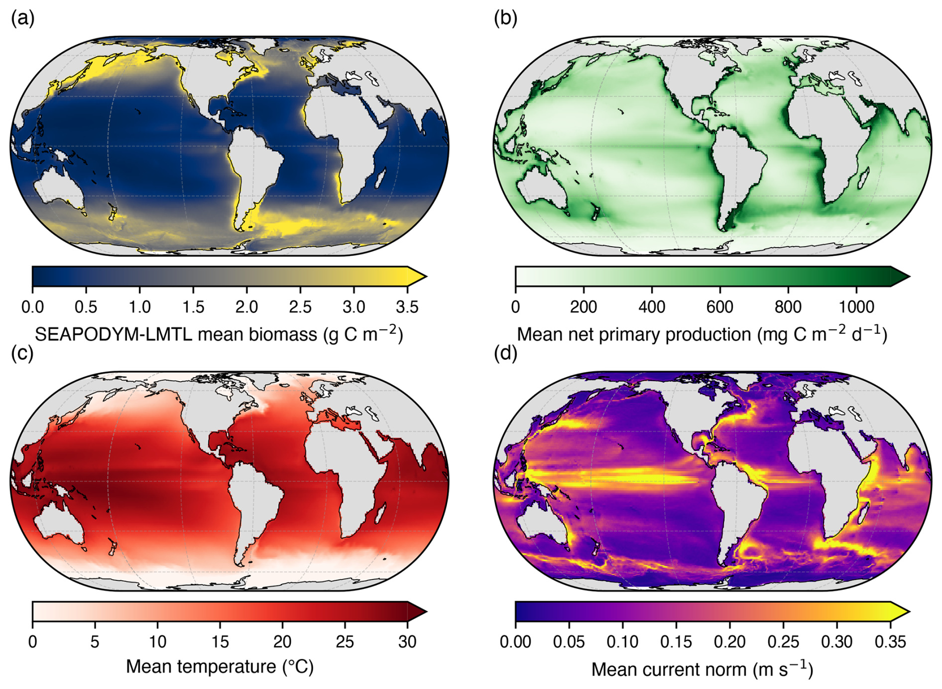
Figure 1 Global ocean maps of the time-mean forcing and the reference biomass, averaged over 2000 to 2019. (a) Mean mesozooplankton biomass of the operational SEAPODYM-LMTL product, the two-dimensional reference that SeapoPym is compared against in Fig. 4. (b) Mean vertically integrated NPP. (c) Mean temperature of the epipelagic layer. (d) Mean current norm of the epipelagic layer.

For the sensitivity and twin experiments, the model is run at the location of six existing observation stations chosen to span a large temperature and primary-production range (Fig. 2). In order of increasing temperature, these are the Barents Sea (BARENTS, 75° N, 40° E), a subarctic northeast Pacific location in the Line P region (PAPA, 50° N, 132° W), the Bay of Biscay (BISCAY, 45.5° N, 4° W), the Canary region (CANARY, 30° N, 13° W), the Bermuda Atlantic Time-series Study site (BATS, 32° N, 64° W) and the Hawaii Ocean Time-series station ALOHA (HOT, 23° N, 158° W). Seasonality does not follow mean temperature alone across these stations. HOT and BATS share a similar mean temperature and productivity, yet the seasonal range of their forcing differs, with a primary-production inter-quartile range about twice as wide at BATS as at HOT (Fig. 2).

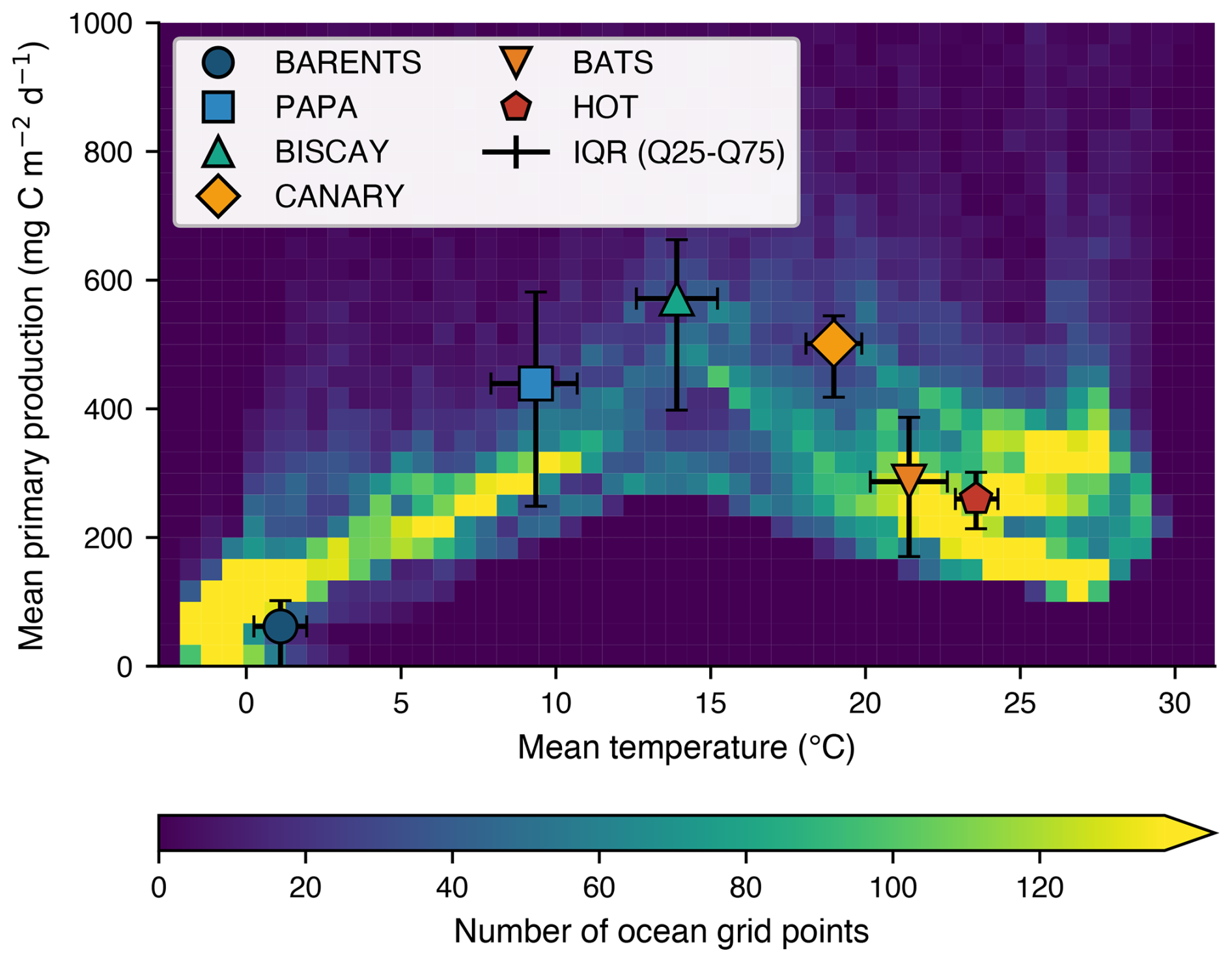
Figure 2 The six stations placed in the global temperature and primary-production space. The color field is a two-dimensional histogram of the ocean grid cells, binned by their 2000 to 2019 mean temperature and mean NPP, the color giving the number of cells in each bin. Each marker is the mean position of one station, and the bars span its interquartile range (25th to 75th percentile) in temperature (horizontal) and in production (vertical) over the same period. Station color encodes mean temperature from cold blue to warm red, a convention kept across every figure.

SeapoPym does not simulate transport. It is therefore necessary to verify whether this simplification is acceptable. To determine whether the resulting error is significant or negligible, we compare it to the existing discrepancy between the operational SEAPODYM-LMTL product and in-situ observations. For this purpose, we use long-term in-situ zooplankton observational data from the two stations for which these time series are freely available: HOT (Station ALOHA) and BATS. These data originate from the Hawaii Ocean Time-series (HOT) and the Bermuda Atlantic Time-series Study (BATS) programs, in the form of total mesozooplankton net samples (200 µm). We retain the epipelagic zooplankton samples and exclude the larger size fraction (>5 mm), consistent with the single epipelagic mesozooplankton group modeled here. The samples are reported as dry-weight biomass per unit volume (mg m⁻³). Dry-weight biomass is converted to carbon using a uniform factor of 0.4, since carbon represents approximately 40 % of zooplankton dry weight (Omori, 1969). This conversion factor is used for both stations. This value is then multiplied by the epipelagic-layer thickness (1.5 Z_eu, Sect. 2.1), taken from the product's time-varying euphotic depth, to obtain carbon biomass per unit area (in g C m⁻²), which is directly comparable to the model results. These observations serve only to compare the models' order of magnitude to the in-situ zooplankton observations (Sect. 2.4) rather than for calibration.

2.4 Implementation validation and inter-model differences

The first validation experiment for the SeapoPym model compares the model's convergence toward the analytical solution $B_{\mathrm{eq}}=R/\mathit{\lambda }$ (Sect. 2.1, Appendix A) under constant forcing. This experiment is conducted at four different temperatures (0, 10, 20 and 30 °C) and a fixed NPP of 300 mg C m⁻² d⁻¹, and we analyze both the absolute difference at equilibrium and the time required to reach that equilibrium. The biomass starts from zero, and we take the time to equilibrium as the time to come within 1 % of the analytical steady state.

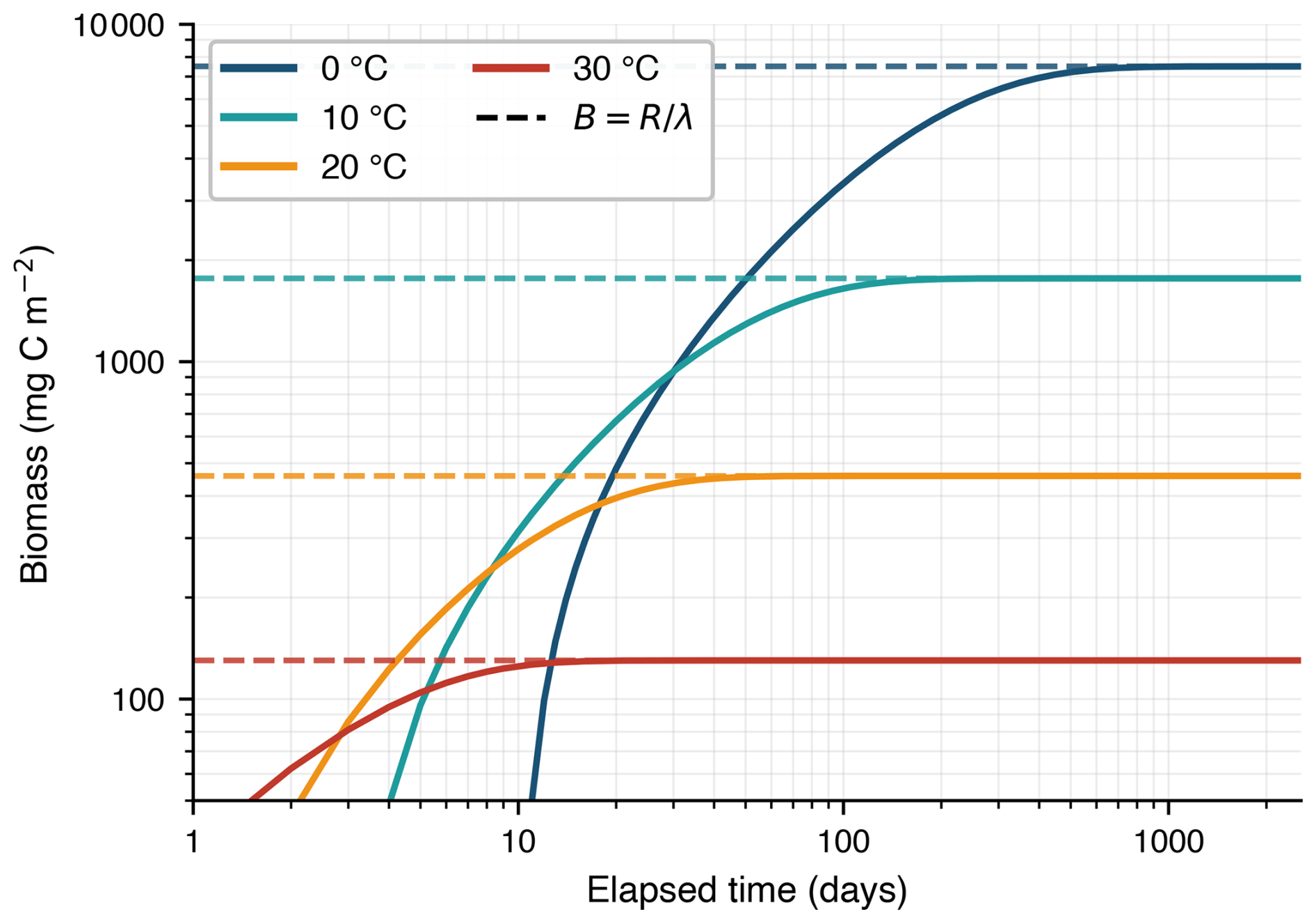
Figure 3 Convergence of the SeapoPym biomass to its analytical steady state under constant forcing. Each solid line is the simulated biomass at one of four constant temperatures (0, 10, 20 and 30 °C), with NPP held at 300 mg C m⁻² d⁻¹, and the matching dashed line is the analytical equilibrium $B_{\mathrm{eq}}=R/\mathit{\lambda }$ (Appendix A). Line color encodes temperature. Both axes are logarithmic. The biomass reaches the analytical value at every temperature, within 0.01 %. The time to approach it lengthens as temperature falls, reaching within 1 % in about fifteen days at 30 °C and about two years at 0 °C.

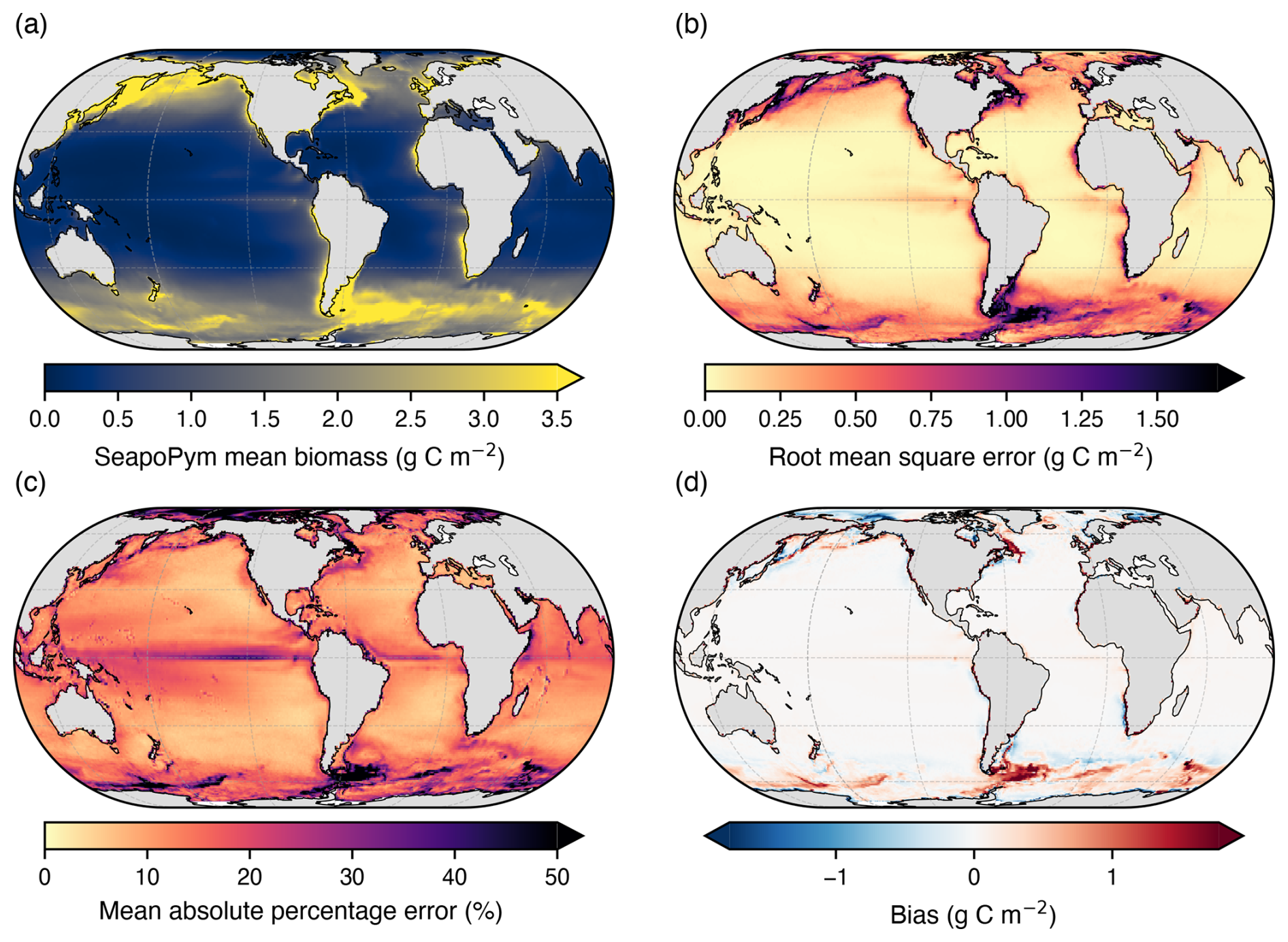
Figure 4 Effect of neglecting transport, shown as SeapoPym (0D) against the operational SEAPODYM-LMTL product (2D), as time means over 2000 to 2019. (a) SeapoPym mean biomass, on the same scale as the reference biomass in Fig. 1a. (b) Root mean square error between the two models. (c) Mean absolute percentage error, the difference taken relative to the local biomass. (d) Bias, the mean signed difference of SeapoPym minus the 2D reference. The difference is largest along the western-boundary currents and the Antarctic Circumpolar Current and in cold high-latitude waters, and smallest in the warm subtropical gyres.

The second experiment compares SeapoPym with the operational SEAPODYM-LMTL product, which includes transport, over the global ocean and the 2000 to 2019 period (Sect. 2.3). This comparison does not separate the effect of transport from that of the re-implementation. We quantify this difference at each grid cell with three complementary metrics (Eqs. 1–3), mapped over the global ocean in Fig. 4. Each metric compares the SeapoPym biomass ${\widehat{y}}_i$ with the reference biomass y_i from SEAPODYM-LMTL, at time step i among the n steps of the series. The bias is the mean signed error, so opposite differences cancel and it can stay near zero even where the two models differ most. The root mean square error (RMSE) does not cancel in this way and measures the magnitude of the difference, giving more weight to large errors. The mean absolute percentage error (MAPE) expresses the difference relative to the local biomass, which matters where biomass is low.

$$\begin{array}{}\text{(1)}& {\displaystyle }\mathrm{bias}={\displaystyle \frac{\mathrm{1}}{n}}\sum _{i=\mathrm{1}}^n({\widehat{y}}_i-y_i)\text{(2)}& {\displaystyle }\mathrm{RMSE}=\sqrt{{\displaystyle \frac{\mathrm{1}}{n}}\sum _{i=\mathrm{1}}^n({\widehat{y}}_i-y_i{)}^{\mathrm{2}}}\text{(3)}& {\displaystyle }\mathrm{MAPE}={\displaystyle \frac{\mathrm{100}}{n}}\sum _{i=\mathrm{1}}^n{\displaystyle \frac{|{\widehat{y}}_i-y_i|}{\left|y_i\right|}}\end{array}$$

To assess whether this difference is significant, we compare it to the discrepancy already existing between the operational SEAPODYM-LMTL product and in-situ observations. At the HOT and BATS stations, where in-situ time series are available, we use the root mean square error to quantify the two discrepancies of the operational SEAPODYM-LMTL product, one with the SeapoPym model and one with the in-situ observations (Fig. 5). We then calculate their ratio, allowing us to place the inter-model difference in the context of the gap between the operational SEAPODYM-LMTL product and the in-situ observations. This comparison focuses solely on the order of magnitude.

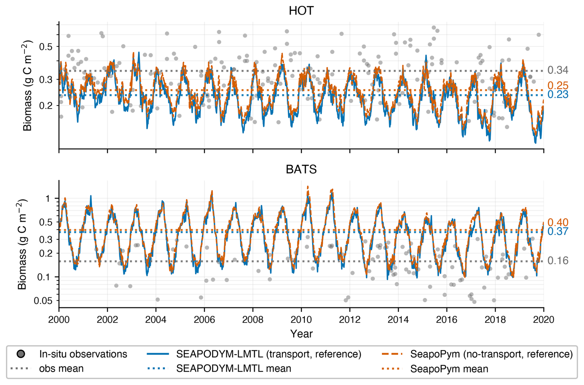
Figure 5 Model biomass against in-situ observations at the two stations with open long-term records, HOT (top) and BATS (bottom). Grey dots are the daily-mean in-situ mesozooplankton biomass, clipped to the 5th to 95th percentile. The solid blue line is the operational SEAPODYM-LMTL product and the dashed orange line is SeapoPym (without transport), both driven by the same forcing and parameters. The dotted horizontal lines mark the time-mean of each series, with their values printed at the right. The y-axis is logarithmic and biomass is in g C m⁻². The two model means nearly coincide while the observed mean sits apart, so the difference between the models, which is due to transport and a different implementation, is five to seven times smaller than the gap between the operational SEAPODYM-LMTL product and the observations.

2.5 Sobol sensitivity analysis

A Sobol sensitivity analysis makes it possible to determine what each parameter controls prior to calibration. It is a global, variance-based method that apportions the variance of a model output among the parameters. It is widely used to identify and rank the driving factors of environmental models (Pianosi et al., 2016; Sobol', 2001). For each parameter, it provides a first-order index S₁, representing the fraction of output variance attributable to that parameter alone, as well as a total index S_T, that represents the fraction attributable to that parameter and all its interactions with others. The difference S_T−S₁ corresponds to the portion of a parameter's influence exerted only in combination with other parameters, isolated through variance decomposition (Saltelli, 2002). The analysis relies on output variance, a quantity independent of the cost function minimized during the optimization (Sect. 2.6).

We run SeapoPym at the six station locations (Sect. 2.3), with the two-year spin-up used throughout, and we vary the five biological parameters over the same ranges as the twin experiments (Sect. 2.6). The result of a sensitivity analysis depends on the chosen descriptors (Pianosi et al., 2016), so we reduce each simulation to two complementary scalars. The first descriptor is the base-10 logarithm of the mean biomass, which measures the overall level, taken in logarithm because the mean spans several orders of magnitude across parameters sets. The second descriptor is the day of year of the biomass maximum, which measures the timing of the seasonal peak. We compute the indices separately at each station location, so that any dependence of the sensitivity on the environment is visible.

We compute the Sobol indices with the SALib library (Herman and Usher, 2017; Iwanaga et al., 2022). Its Saltelli sampler sample_sobol generates the sets of parameter values at which the model is run, and its estimator sobol.analyze returns S₁ and S_T with 95 % bootstrap confidence intervals. For the D=5 parameters, a base sample size N yields N(D+2) parameter sets, one per model run. Only first- and total-order indices are computed, which is what fixes the count to N(D+2). The Saltelli sample and the bootstrap confidence intervals both use a fixed random seed, so the design and the reported intervals are reproducible. Rather than fixing N in advance, we choose it by a convergence test on the indices. We raise N through a doubling sequence, re-estimate the indices at each value, and stop at the smallest N that meets two conditions. The first follows Sarrazin et al. (2016) and requires precision: the half-width of the 95 % bootstrap confidence interval of each index must stay below 0.05. The second requires stability: each index must change by less than 0.05 from the previous N. Both conditions are first met at N=8192, that is N(D+2) = 57 344 model runs.

2.6 CMA-ES: parameter optimization

We assess identifiability with twin experiments. From the reference parameters (Table 1) we simulate the synthetic observations at each station over the 2000 to 2019 analysis period, then we use the optimizer to recover those parameters by fitting these synthetic observations either separately or together. Each candidate runs its own two-year spin-up over 1998 and 1999 within a full 1998 to 2019 integration, and the cost is scored on the 2000 to 2019 analysis window (Sect. 2.3). Because the synthetic observations are produced by the transport-free model itself and used without added noise, the target contains no transport signal, and an exact recovery is possible in principle. Twin experiments of this kind were used on the same model family by Delpech et al. (2020) for the micronekton energy-transfer coefficients.

We recover the parameters with CMA-ES, that is an algorithm of adaptation evolution strategy using the covariance matrix (Hansen and Ostermeier, 2001; Hansen, 2016). CMA-ES is a derivative-free method that adapts a multivariate normal search distribution to the local shape of the cost, which suits a smooth but possibly ill-conditioned cost without requiring its gradient. We use pycma, its reference implementation (Hansen et al., 2019), with the five parameters mapped to the unit box (linearly normalized between 0 and 1) from the search ranges of Table 1 and the standard CMA-ES settings. The default population size, i.e. the number of parameter sets to test in one iteration, is defined by $\lfloor \mathrm{4}+\mathrm{3}\ln D\rfloor =\mathrm{8}$ for D=5 parameters (Hansen, 2016). The initial step size is σ₀=0.30, and candidate solutions that leave the unit box are mapped back into it by a smooth transformation, pycma's default boundary handling. The search stops on the standard CMA-ES convergence criteria, when the step size and the spread of the cost fall below pycma's default tolerances (step-size tolerance 10⁻⁴). A generation cap is used solely as a safety measure, as it is never reached during the experiments.

A single optimization can settle in a local optimum that depends on its starting point, so we repeat the search from twenty random starts (seeds 0 to 19), hereafter called restarts, and keep the best. We assess identifiability by comparing the parameters recovered by the run achieving the best score with the reference. Parameters matching the reference are well constrained by the synthetic observations, whereas a recovered parameter set that departs from the reference while it gets the best score suggests a problem of equifinality (Beven, 2006).

The cost function is the root mean square error normalized by the mean of the synthetic observations (NRMSE). Following Eq. (2), $\widehat{y}$ refers to the simulated biomass and y refers to the synthetic observations, so that stations with different biomasses enter on a comparable scale. For the joint experiment, the cost function is the mean of the per-station NRMSE. We conduct seven experiments, each of the six stations individually and one joint experiment (MERGED) that combines all six. The recovered parameter values are reported with the results.

3 Results

3.1 Implementation validation and the impact of transport

Under constant forcing, the simulated biomass converges to the analytical steady state $B_{\mathrm{eq}}=R/\mathit{\lambda }$ at every temperature tested, the relative departure falling below 0.01 % given a long enough integration (Fig. 3). It reaches within 1 % of this equilibrium in about fifteen days at 30 °C and about two years at 0 °C, the adjustment slowing as temperature falls. This slow adjustment in cold water sets the two-year spin-up used throughout the study, which brings even the coldest water to within about 1 % of equilibrium, so the analysis at every station begins from a near-equilibrium state.

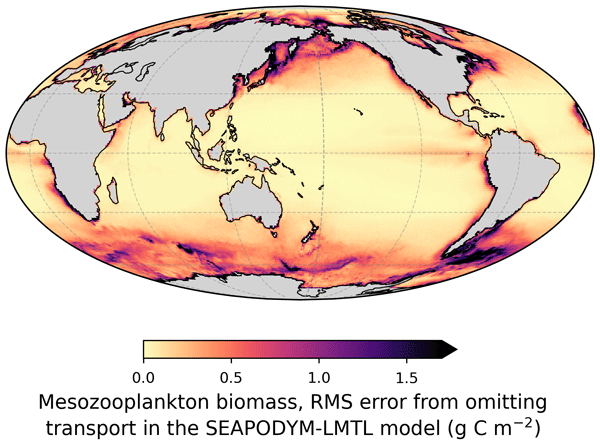
The difference between SeapoPym and the operational SEAPODYM-LMTL product measures the combined effect of omitting transport and the re-implementation. As Fig. 4 shows, it is non-uniform across the ocean. In absolute terms, the RMSE is largest where currents and gradients are strong, along the Gulf Stream, the Kuroshio and the Antarctic Circumpolar Current, and in cold high-latitude waters where the long life cycle of zooplankton leaves the biomass exposed to advection for a longer period. The MAPE, calculated relative to local biomass, reduces the weights of these high-biomass currents and instead highlights regions of lower biomass, particularly around the equator in the Pacific, Indian and Atlantic Oceans. The bias introduces a directional dimension. Its opposite-signed fronts mark neighboring areas where the 0D model shows higher and lower biomass than the two-dimensional (2D) reference, a dipole consistent with biomass displaced by currents, such as at the confluence in the South Atlantic between the warm Brazil Current and the cold Malvinas Current. This signed pattern is consistent with transport redistributing biomass between adjacent regions, although a static difference map does not resolve the displacement itself.

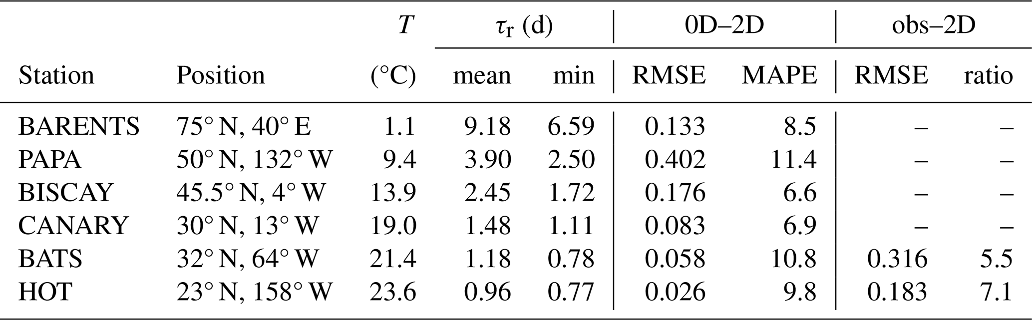
To assess the significance of this difference, we compare it to the discrepancy already existing between the operational SEAPODYM-LMTL product and the in-situ observations. At HOT and BATS stations the difference between the 0D and 2D models is five to seven times smaller than the gap between the operational SEAPODYM-LMTL product and the observations (Fig. 5, see Table B1 for station-specific values). The two models yield similar results, yet both deviate from the observations in terms of amplitude: they underestimate values at HOT and overestimate them at BATS. This justifies the use of local 0D optimization in these regimes. This finding applies to both HOT and BATS, which are warm-water oligotrophic stations with in-situ measurement series. The comparison focuses solely on magnitude, as the observations are not used for calibration.

3.2 Sobol sensitivity analysis

Sensitivity analysis of biomass magnitude reveals a distribution of roles (Fig. 6). This magnitude is determined by energy transfer E and the two mortality parameters, with the balance between these factors shifting along the temperature gradient. First-order indices for E and λ₀ decrease from the coldest station to the warmest station, whereas the index for γ_λ rises from a value near zero at BARENTS to approximately 0.6 at HOT. The thermal term γ_λ is inactive near the reference temperature but dominant in warm waters. Recruitment parameters have no impact on this magnitude, and for this descriptor, the indices are additive, summing to one at each station.

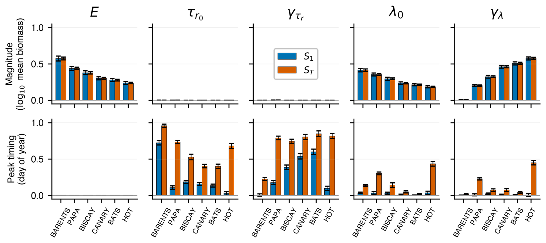
Figure 6 Sobol sensitivity indices of the biomass to the five biological parameters at the six stations, ordered from coldest to warmest. The rows are the two output descriptors, the magnitude (base-10 logarithm of the mean biomass, top) and the seasonal peak timing (day of year of the maximum, bottom). The columns are the five parameters E, ${\mathit{\tau }}_{{\mathrm{r}}_{\mathrm{0}}}$, ${\mathit{\gamma }}_{{\mathit{\tau }}_{\mathrm{r}}}$, λ₀ and γ_λ. In each panel the blue bars are the first-order index S₁, the share of output variance due to that parameter alone, and the orange bars the total-order index S_T, which adds its interactions with the other parameters. Error bars are 95 % bootstrap confidence intervals. The indices are computed from a Saltelli design of N=8192 base samples, that is 57 344 model runs at each station. The magnitude is governed by the energy transfer and the two mortality parameters, the peak timing by the two recruitment parameters.

The peak timing is governed by the recruitment parameters, while energy transfer has no effect. At BARENTS, BISCAY, CANARY and BATS the first-order indices sum to 0.6 to 0.8, so recruitment acts mostly directly, whereas that sum falls to 0.33 at PAPA and 0.17 at HOT, so interactions carry most of the timing variance. The two recruitment parameters respond to temperature differently. At BARENTS the first-order index of ${\mathit{\tau }}_{{\mathrm{r}}_{\mathrm{0}}}$ reaches 0.72, and its total-order index falls with warming, from 0.96 at BARENTS to 0.40 at BATS. The first-order index of ${\mathit{\gamma }}_{{\mathit{\tau }}_{\mathrm{r}}}$ rises over the same gradient, from near zero at BARENTS to 0.60 at BATS. HOT departs from both trends: the first-order indices of ${\mathit{\tau }}_{{\mathrm{r}}_{\mathrm{0}}}$ and ${\mathit{\gamma }}_{{\mathit{\tau }}_{\mathrm{r}}}$ fall below 0.1 while their total-order indices reach 0.68 and 0.82, so recruitment acts on the timing almost entirely through interactions.

Taken together, these two descriptors distinguish the respective roles of the parameters: magnitude is determined by energy transfer and mortality, whereas timing is determined by recruitment. At steady state, biomass results from a multiplicative combination of the parameters (Appendix A). Therefore, its logarithm is expressed as a sum of distinct terms: $\log B=\log E-\log {\mathit{\lambda }}_{\mathrm{0}}-{\mathit{\gamma }}_{\mathit{\lambda }}\stackrel{\mathrm{‾}}{T}+\log \mathrm{NPP}$, where $\stackrel{\mathrm{‾}}{T}$ and NPP are fixed by the station and where recruitment does not appear. The sensitivity analysis confirms this simplified scheme, showing additive indices for magnitude and a negligible effect of recruitment. However, sensitivity does not imply identifiability: knowing what each parameter controls does not determine whether it can be estimated from the data. This is a point that is demonstrated by the twin experiments presented in Sect. 3.3.

3.3 Twin experiments: convergence and parameter recovery

We read parameter recovery from the best restart of each experiment (Table 2). At the cold stations BARENTS, PAPA and BISCAY, and in the joint MERGED experiment, all five parameters are recovered to better than 0.1 % of the reference, recruitment included. At the warm stations CANARY and BATS the energy transfer and the two mortality parameters are recovered to the same precision, but the two recruitment parameters ${\mathit{\tau }}_{{\mathrm{r}}_{\mathrm{0}}}$ and ${\mathit{\gamma }}_{{\mathit{\tau }}_{\mathrm{r}}}$ miss the reference by 40 % to 160 %.

Table 2 Parameter recovery in the twin experiments, where the optimizer recovers known parameters from synthetic observations that the model generated itself, taking the best of twenty CMA-ES restarts. Each entry is the signed relative divergence of a recovered parameter against its synthetic-observation reference, in percent. The last column is the achieved cost (mean-normalized NRMSE). The cold stations and MERGED recover all five parameters, CANARY and BATS miss the two recruitment parameters, and HOT does not reach the optimum. A large error next to a near-zero cost is equifinality.

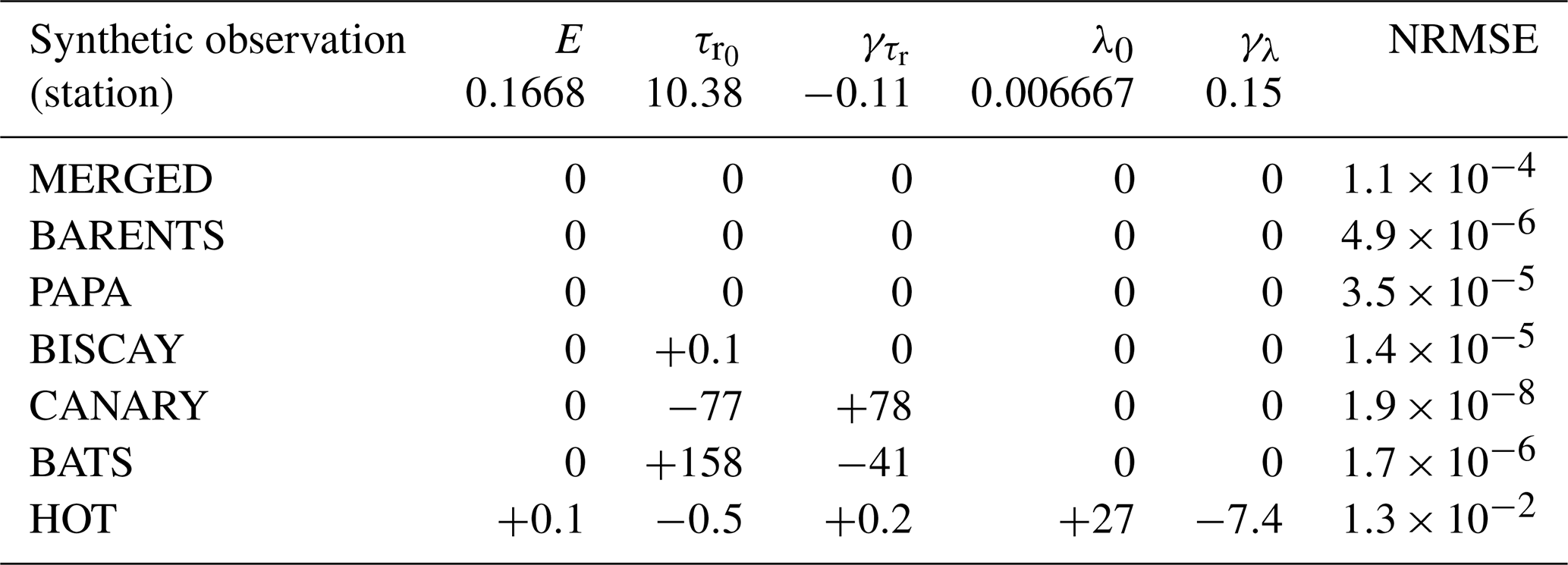
To validate convergence we use the cost reached by the experiments that recover the parameters as a benchmark. The cold stations and MERGED reach an NRMSE of order 10⁻⁴ (Table 2), and CANARY and BATS reach it as well, so both converged (Fig. 7). HOT's best restart, by contrast, stays near 10⁻², two orders of magnitude above, so none of its twenty restarts converged and we leave HOT out of the recovery analysis.

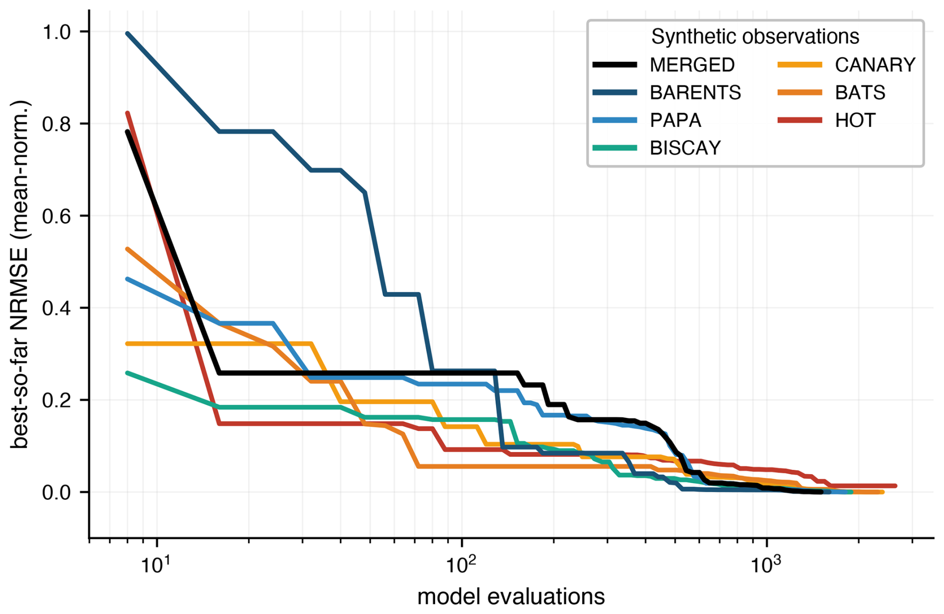
Figure 7 CMA-ES convergence for the seven twin experiments, each the best of twenty random restarts. Each line is the best-so-far cost against the number of model evaluations, for the six single-station experiments and the joint MERGED experiment. The cost is the NRMSE between the recovered and the synthetic biomass, normalized by the mean of the target series. The x-axis is logarithmic. Station color follows the cold-to-warm convention and MERGED is black. Every experiment drives the cost to near zero, about 10⁻⁴, except HOT, which floors near 10⁻². Because the target is the model's own output a zero cost is attainable, so the HOT residual likely reflects an incomplete search rather than a structural floor.

Three conclusions follow. At CANARY and BATS the search reaches the cost of a full recovery yet leaves the recruitment parameters far from the reference, so a good fit does not identify the parameters, the equifinality of Beven (2006). At the cold stations, by contrast, the search both converges and recovers all five parameters. In MERGED, the joint search over the six stations converges and recovers every parameter to better than 0.1 % of the reference, so the non-identifiable warm stations do not degrade the joint estimate.

4 Discussion

The first question this study addressed is whether a transport-free re-implementation is a valid basis for parameter optimization. SeapoPym converges to the analytical steady state of the reference equations, and its departure from the operational SEAPODYM-LMTL product is small enough for local 0D optimization to be valid, at least at the two warm stations where in-situ observations allow that comparison. The second question is whether zooplankton observations carry enough information to recover the five biological parameters of the SEAPODYM-LMTL model. Using the SeapoPym model coupled to a CMA-ES optimizer, we found that the answer depends on the environmental regime sampled. The energy-transfer and mortality parameters were recovered at every station where the search converged, whereas the recruitment parameters were recovered only in cold water.

The influence of advection on zooplankton distribution has long been recognized and is often pronounced, particularly in regions characterized by intense physical dynamics, such as frontal zones, upwelling systems, and areas with strong currents (e.g., Banse, 1964; Edvardsen et al., 2006; Mackas and Coyle, 2005). Our comparison with the operational SEAPODYM-LMTL product confirms that transport cannot be ignored in such areas, especially when these conditions prevail in cold-water environments. This result aligns with theoretical predictions stating that physical transport becomes significant when biological timescales exceed physical retention timescales. This scenario is more likely in cold waters, where zooplankton generation times can exceed one year (Conover, 1988; Kosobokova, 1999; Daase et al., 2013). Nevertheless, the version of our model that omits transport remains suitable for simulating and estimating mesozooplankton parameters in most warm- and temperate-water regions, outside of localized dynamic zones. This is the case at our six stations, where the 0D-to-2D difference stays between 6 % and 12 % (Table B1). This difference is smaller than the model-observation gap only where we could measure that gap, at the two warm stations HOT and BATS. Confirming it in cold water would require in-situ series there.

The Sobol sensitivity analysis assigns a distinct role to each parameter: energy transfer and the two mortality parameters govern the magnitude of the biomass, while the two recruitment parameters govern the timing of the seasonal peak, with their relative predominance depending on the temperature regime. This division shapes what a calibration against real data can and cannot separate. At steady state the mean biomass depends on the energy transfer E, the mortality λ, and the primary production through the ratio $\frac{E\times \mathrm{NPP}}{\mathit{\lambda }}$ (Appendix A), so these three are confounded in the magnitude. A bias in the NPP forcing magnitude could therefore be absorbed into biased estimates of E and λ, indistinguishable in the mean biomass from a genuine parameter error. The recruitment parameters play an analogous role for timing, absorbing errors in the seasonal phase of the forcing. Our twin experiments recover E and the mortality parameters because the forcing is identical for the target and the candidates. Against uncertain forcing these same parameters could instead take values that compensate for it, so their calibrated estimates should be interpreted as effective quantities rather than independently identified ones.

The same reasoning applies to transport. Since the synthetic observations are generated by SeapoPym, they contain no transport signal to be absorbed. These twin experiments therefore do not allow us to assess whether the optimized parameters would take biased values to compensate for the omission of transport. Assessing this would require the same experiment with a target that carries a transport signal, such as the operational product. The recovery presented here should not be interpreted as proof that the estimates would remain unbiased in that case.

At the cold stations the mean recruitment age exceeds two daily cohorts (Table B1), and the two recruitment parameters are recovered. At CANARY and BATS, where the mean recruitment age is close to one daily cohort, the recruitment parameters are not recovered, even though the fit reaches the same cost as at the cold stations. Consequently, the quality of the fit alone does not guarantee the validity of the calibration. Sensitivity does not imply identifiability either, since at BATS the first-order index of ${\mathit{\gamma }}_{{\mathit{\tau }}_{\mathrm{r}}}$ on the peak timing reaches 0.60. A likely reason lies in how recruitment is discretized. Age classes are one time step wide, and a class is completely absorbed into the biomass (Appendix A), so two recruitment ages within the same age class produce the same recruitment and the cost changes in steps rather than continuously. The recruitment age also decreases exponentially with temperature, so only one or two age classes are resolved in warm water. Crossing a class boundary there demands either a wider temperature range or a larger parameter change than at the cold stations. This warm-water equifinality would therefore stem from both the exponential behavior of recruitment and the numerical solution the model uses. A smoother recruitment, or a finer time and age step, would smooth the cost function, but we have not tested whether either restores identifiability. Recruitment parameters must therefore be determined from independent data or estimated in conjunction with an informative cold station, as demonstrated by the MERGED experiment.

These results have direct implications for observing-system design. Recovering all five parameters requires sampling at least one cold-water regime, because recruitment is identifiable there. A single cold station, sampled across its full seasonal range, constrained the five parameters as well as the six stations combined. What matters is the information content of the regime, not the number of stations. The cold station must also have weak enough currents for the 0D approximation to hold, as at BARENTS, PAPA and BISCAY, where the 0D-to-2D difference is of the same order, in relative terms (MAPE), as at the warm stations. Cold but strongly advective regions carry the same seasonal signal, but exploiting it would require a version of the model that resolves transport.

These findings are a best case. The synthetic observations are noise-free, complete at every time step, and driven by the exact forcing, whereas in-situ series are sparse and irregular and the forcing carries its own error. All three will lower identifiability and widen parameter uncertainty in real applications. Working with such observations will also require a cost function that represents their error, such as a Gaussian likelihood that weights the misfit by the observation-error variance, or a log-normal likelihood suited to the positive, skewed distribution of plankton biomass (Schartau et al., 2017). A second limitation is our diagnosis of equifinality. We identified it from the best restart alone, which showed that parameter sets far from the reference reached the same cost, but this single optimum does not reveal the whole family of parameter sets that fit the observations equally well. Mapping that family would require sampling the parameter space rather than a single optimum, either as a behavioral ensemble drawn by random sampling (Beven and Binley, 1992) or as a Bayesian estimate of the parameter posterior (Tarantola, 2005).

The first step beyond this study is to repeat these experiments under realistic conditions, as an observing system simulation experiment in which measurement error, temporal gaps, and forcing uncertainty are added to the synthetic observations (Hoffman and Atlas, 2016). Such an experiment would show how much of the identifiability reported here still holds under those conditions. It would also let us vary the sampling effort, which we held fixed, since every station used the same complete twenty-year record. We do not know whether a long continuous record outperforms shorter records spread over several stations, nor where along the temperature gradient recruitment identifiability breaks down. The second step is to calibrate the model against real data. The long-term series at HOT and BATS are complete, but this study shows that they cannot constrain recruitment. A cold and weakly advective station is needed as well. The COPEPOD database is a logical candidate, although a long-term series in cold water would constrain recruitment more directly. The SeapoPym framework is built for both steps.

5 Conclusions

We presented here SeapoPym, an open-source Python re-implementation of the SEAPODYM-LMTL model for mesozooplankton biology. It is coupled with a modular framework in which the model, observations, cost function, and optimizer are interchangeable components. We validated this re-implementation against the operational SEAPODYM-LMTL product and its analytical steady state. We determined the roles of the five parameters using a Sobol analysis, then tested their identifiability using twin experiments at six station locations with different environmental conditions. The difference between the 0D and 2D models, which combines the omission of transport and the re-implementation, ranges from 6 % to 12 % of the simulated biomass at all six stations (Table B1). At HOT and BATS, the only stations with in-situ records, it is five to seven times smaller than the discrepancy between the model and the observations, so it is second-order there. The 0D model therefore serves as a valid test bed for assessing parameter identifiability where transport is a second-order effect.

The identifiability of the parameters depends on the environmental conditions observed. In the twin experiments, the energy-transfer and mortality parameters were correctly estimated at every station where the search converged, while the recruitment parameters were estimated only under cold-water conditions. At warm stations, the optimization reaches parameter sets far from the reference that minimize the cost as well as at the cold stations. Cost convergence, therefore, does not imply that the parameters are correctly estimated. A single cold station constrained all five parameters as well as the six stations combined. Parameter recovery is therefore determined by the information content of the sampled regime, not by the number of stations. In locations where the difference between the 0D and 2D models is second-order, the 0D model can be calibrated using observations made under cold, low-current conditions, where recruitment is informative. In the absence of such cold observations, recruitment parameters must be set or constrained based on independent, process-based knowledge.

The twin experiments use noise-free observations, complete at every time step, generated by the transport-free model itself and driven by the exact forcing. The identifiability they show is therefore a best case, and it leaves open whether the parameters would absorb the missing transport once the target contains it. In-situ series are sparse and irregular, and the forcing carries its own error, so real conditions will reduce the identifiability. One warm station, HOT, did not converge to the low cost reached at the other stations and departed from them for reasons that remain open. Calibrating the model against real data will require a cold, weakly advective station with a long time series, where recruitment is informative and the 0D approximation holds, and a cost function that represents observational error.

Appendix A: Underlying model equations

The full SEAPODYM-LMTL model resolves several functional groups across three vertical layers, with diel vertical migration linking the layers (Sect. 2.1, Lehodey et al., 2010). The equations below describe the single epipelagic mesozooplankton group studied here. The functional groups are not coupled to one another, each driven independently by primary production, and the epipelagic group does not migrate, so neither inter-group terms nor diel vertical migration appear here. The group is represented by two coupled state variables, an age-structured production field p(t,τ) and an age-aggregated biomass pool B(t). All equations are written in continuous form, the discretization of time and age being introduced only in the numerical-solution part.

A1 Biomass

The biomass B [g C m⁻²] follows the balance between the recruitment flux R and mortality:

$$\begin{array}{}\text{(A1)}& {\displaystyle \frac{\mathrm{d}B}{\mathrm{d}t}}=R\left(t\right)-\mathit{\lambda }\left(t\right)B\left(t\right)\end{array}$$

where R [g C m⁻² d⁻¹] is the recruitment flux from the aging production field (defined below) and λ [d⁻¹] is the mortality rate. At steady state this gives the equilibrium biomass $B_{\mathrm{eq}}=R/\mathit{\lambda }$. Mortality rises exponentially with temperature:

$$\begin{array}{}\text{(A2)}& \mathit{\lambda }\left(t\right)={\mathit{\lambda }}_{\mathrm{0}}\exp \left({\mathit{\gamma }}_{\mathit{\lambda }}\stackrel{\mathrm{‾}}{T}\right(t\left)\right)\end{array}$$

where λ₀ is the mortality rate at the reference temperature and γ_λ [°C⁻¹] its thermal sensitivity. The temperature entering the metabolic terms is the normalized temperature of the SEAPODYM-LMTL model (Lehodey et al., 2010), after the metabolic theory of Gillooly (2000) and Gillooly et al. (2002),

$$\begin{array}{}\text{(A3)}& \begin{array}{rl}& \stackrel{\mathrm{‾}}{T}\left(t\right)={\displaystyle \frac{T\left(t\right)}{\mathrm{1}+T\left(t\right)/\mathrm{273}}},T\left(t\right)=max\left(T_{\mathrm{env}}\right(t),T_{\mathrm{ref}}),\\ & T_{\mathrm{ref}}=\mathrm{0}\mathit{°}\mathrm{C},\end{array}\end{array}$$

where T_env is the temperature forcing (Sect. 2.3) and T_ref the reference temperature, with T floored at T_ref so that the recruitment age cannot exceed the maximum age the model resolves (below).

A2 Production

The production field p(t,τ) [g C m⁻² d⁻¹] describes how production is distributed across age τ. It ages at unit velocity and is conserved while it ages, following the loss-free McKendrick-Von Foerster transport equation (McKendrick, 1926; Von Foerster, 1959):

$$\begin{array}{}\text{(A4)}& {\displaystyle \frac{\partial p}{\partial t}}+{\displaystyle \frac{\partial p}{\partial \mathit{\tau }}}=\mathrm{0}\end{array}$$

Its dynamics are set by two boundaries, a source at age zero and a sink at the recruitment age. At age zero, a fraction E of NPP is injected (the source):

$$\begin{array}{}\text{(A5)}& p(t,\mathit{\tau }=\mathrm{0})=E\mathrm{NPP}\left(t\right),\end{array}$$

with NPP the net primary production [g C m⁻² d⁻¹] and E the dimensionless transfer efficiency between primary production and zooplankton production. The sink at the recruitment age is described next.

A3 Recruitment

Production is recruited into the biomass pool when it reaches the temperature-dependent recruitment age τ_r(t):

$$\begin{array}{}\text{(A6)}& {\mathit{\tau }}_{\mathrm{r}}\left(t\right)={\mathit{\tau }}_{{\mathrm{r}}_{\mathrm{0}}}\exp \left({\mathit{\gamma }}_{{\mathit{\tau }}_{\mathrm{r}}}\stackrel{\mathrm{‾}}{T}\right(t\left)\right),\end{array}$$

where ${\mathit{\tau }}_{{\mathrm{r}}_{\mathrm{0}}}$ is the recruitment age at the reference temperature (hence the maximum age represented in the model) and ${\mathit{\gamma }}_{{\mathit{\tau }}_{\mathrm{r}}}$ [°C⁻¹] its thermal sensitivity. This sink is an absorbing boundary, $p(t,\mathit{\tau })=\mathrm{0}$ for τ>τ_r(t), and the recruitment flux feeding the biomass is the production reaching that age:

$$\begin{array}{}\text{(A7)}& R\left(t\right)=p(t,{\mathit{\tau }}_{\mathrm{r}}(t\left)\right).\end{array}$$

Recruitment moves production from the field p into the pool B, a transfer and not a loss. Mortality acts only on B, through λ, and any loss during development is absorbed into the efficiency E.

A4 Numerical solution

Age and time are discretized into steps Δτ and Δt, and production is carried in discrete cohorts (age classes) indexed by a, advanced over time steps indexed by n. Because production ages at unit velocity, we set $\mathrm{\Delta }t=\mathrm{\Delta }\mathit{\tau }\equiv \mathrm{\Delta }=\mathrm{1}$ d, a Courant number of one, so one time step moves a cohort up by exactly one age class. The number of resolved age classes is set by the maximum recruitment age, about eleven daily classes at the reference temperature (${\mathit{\tau }}_{{\mathrm{r}}_{\mathrm{0}}}=\mathrm{10.38}$ d). Each step then reduces to three operations on the production field, by region of age:

$$\begin{array}{}\text{(A8)}& p_a^{n+\mathrm{1}}=\left\{\begin{array}{lll}E{\mathrm{NPP}}^{n+\mathrm{1}}& a=\mathrm{0}& \text{(source at age zero)}\\ p_{a-\mathrm{1}}^n& \mathrm{0}<a\mathrm{\Delta }<{\mathit{\tau }}_{\mathrm{r}}^{n+\mathrm{1}}& \text{(loss-free aging)}\\ \mathrm{0}& a\mathrm{\Delta }\ge {\mathit{\tau }}_{\mathrm{r}}^{n+\mathrm{1}}& \text{(recruitment)}\end{array}\right.\end{array}$$

The production that crosses the recruitment age (the classes set to zero) feeds the biomass, giving the recruitment flux $R^{n+\mathrm{1}}={\sum }_{a\ge \mathrm{1}}(p_{a-\mathrm{1}}^n-p_a^{n+\mathrm{1}})$. At a Courant number of one these operations are exact, so the production needs no integration scheme. Only the biomass does, because of its mortality term.

The biomass is integrated with an implicit (backward Euler) scheme, evaluating the right-hand side at the new time step:

$$\begin{array}{}\text{(A9)}& B^{n+\mathrm{1}}={\displaystyle \frac{B^n+\mathrm{\Delta }{R}^{n+\mathrm{1}}}{\mathrm{1}+\mathrm{\Delta }{\mathit{\lambda }}^{n+\mathrm{1}}}}.\end{array}$$

This scheme is unconditionally stable. A fully explicit update is not: in warm water and over the high mortality rates explored during the experiments (Sect. 2.5 and 2.6), it produces spurious oscillations and negative biomass. The implicit form lets the whole parameter range be integrated with a single time step.

Appendix B: Per-station summary

Table B1 gathers, for each of the six stations, the mean temperature, the recruitment age at the mean and warmest points of its forcing, the difference between the 0D and 2D models, and, where in-situ records exist, the structural gap between the operational SEAPODYM-LMTL product and the observations.

Table B1 Per-station summary, stations ordered by increasing mean temperature. For each station: position, mean temperature of the epipelagic layer, the recruitment age ${\mathit{\tau }}_{\mathrm{r}}={\mathit{\tau }}_{{\mathrm{r}}_{\mathrm{0}}}\exp \left({\mathit{\gamma }}_{{\mathit{\tau }}_{\mathrm{r}}}\stackrel{\mathrm{‾}}{T}\right)$ (Table 1, Appendix A) at the mean and at the warmest point of the forcing series, in days and equivalently in daily cohorts, the difference between the 0D SeapoPym and the operational SEAPODYM-LMTL product (RMSE and MAPE sampled from the maps of Fig. 4 over 2000 to 2019), and, at the two stations with in-situ records, the structural gap between the 2D reference and the observations (RMSE) with its ratio to the 0D-to-2D difference. RMSE in g C m⁻², MAPE in percent. The ratio is computed from the daily series as in Fig. 5, with the observations clipped to their 5th–95th percentiles.

Appendix C: Abbreviations

The abbreviations and acronyms used in this paper are listed below.

Abbreviation	Definition
0D	Zero-dimensional, the local SeapoPym model with transport neglected
2D	Two-dimensional, the operational SEAPODYM-LMTL product with transport resolved
CMA-ES	Covariance matrix adaptation evolution strategy
CMEMS	Copernicus Marine Environment Monitoring Service
COPEPOD	Coastal and Oceanic Plankton Ecology, Production and Observation Database
GLORYS12	Global ocean reanalysis at $\mathrm{1}/\mathrm{12}$° resolution, the source of the temperature forcing
LMTL	The component of SEAPODYM which models the Low and Mid-Trophic Levels
MAPE	Mean absolute percentage error
NPP	Net primary production
NRMSE	Normalized root mean square error, here normalized by the mean
RMSE	Root mean square error
SEAPODYM	Spatial Ecosystem and Populations Dynamics Model
SeapoPym	The open Python re-implementation of the SEAPODYM-LMTL biology presented here
VGPM	Vertically Generalized Production Model

Appendix D: Workflow overview

Figure D1 gives an overview of the modeling and experimental workflow. Temperature and NPP drive both models, whereas the currents drive only the SEAPODYM-LMTL model (with transport), SeapoPym being transport-free. The figure also shows the in-situ observations, the CMA-ES optimizer, and the four experiments together with the components each one uses.

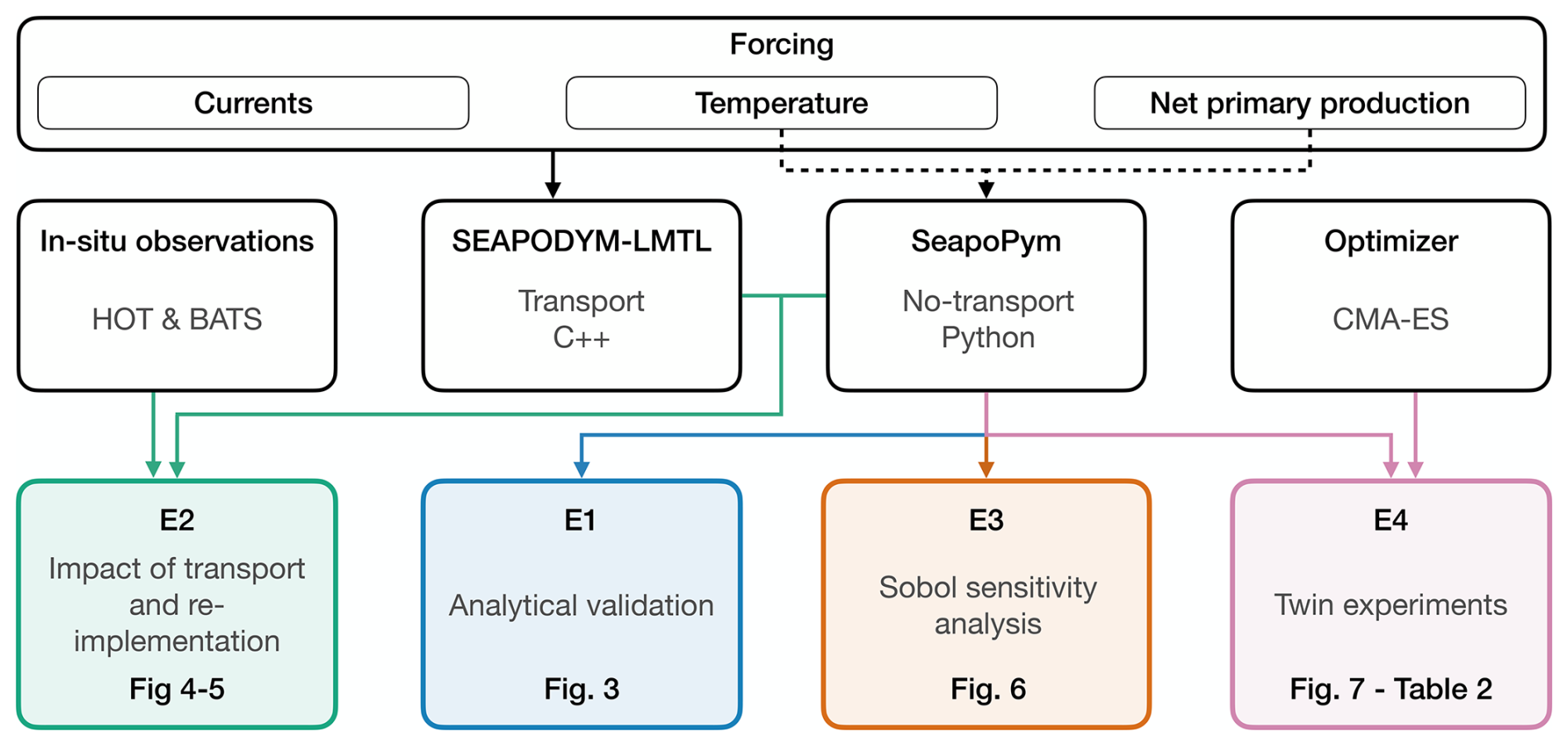
Figure D1 Overview of the SeapoPym modeling and experimental workflow. Temperature and NPP drive both models, whereas the currents drive only the SEAPODYM-LMTL model (with transport, C$++$). The dashed link marks that SeapoPym (without transport, Python) omits the currents. Each experiment is color-coded and linked to the components it uses, with the figures that report it. E1 (analytical validation, Fig. 3) and E3 (Sobol sensitivity analysis, Fig. 6) exercise the SeapoPym model. E2 (impact of transport and re-implementation, Figs. 4–5) compares SeapoPym with the operational SEAPODYM-LMTL product and with the in-situ observations at HOT and BATS. E4 (twin experiments, Fig. 7 and Table 2) recovers the SeapoPym parameters with the CMA-ES optimizer from synthetic observations generated by SeapoPym itself.