
the Creative Commons Attribution 4.0 License.
the Creative Commons Attribution 4.0 License.
 | 08 Sep 2026
A general physiologically driven representation of leaf turnover in grasslands in the QUINCY land surface model (revision: 974a6b7f)

Midori Yajima
Yu Zhu
Lumnesh Swaroop Kumar Joseph
Jinyan Yang
Fabrice Lacroix
Yunpeng Luo
Andreas Schaumberger
Michael Bahn
Sönke Zaehle
Silvia Caldararu
Terrestrial vegetation plays an important role in shaping the Earth's climate due to its control on the global carbon cycle. Understanding and predicting vegetation phenology and biomass turnover into soil organic matter is therefore of great importance for our understanding and quantification of carbon exchange with the atmosphere, which varies seasonally. In the past, models of tree phenology have been developed extensively, but equivalent models for herbaceous ecosystems, which cover a significant area of the terrestrial land surface and provide many ecosystem services to humans, have been much more poorly developed for both the start and the end of season. These limitations may be due to spatially and temporally sparse observational data in grasslands, but more importantly, their distribution across a large range of climatic and environmental conditions, as well as a lack of understanding of underlying processes. It follows that a refined autumn phenology model for grasslands is a necessary component of land surface models (LSMs). Here we present a novel approach to grassland autumn phenology by introducing a general leaf turnover model controlled by environmental conditions into the QUINCY (QUantifying Interactions between terrestrial Nutrient CYcles and the climate system) LSM and show that decoupling leaf senescence from growing season triggers improves site-level carbon dynamics in herbaceous systems globally. We tested the model at 59 sites with differing climates and show that our model was able to reduce errors in gross primary productivity (GPP) predictions as well as in the timing of the onset of leaf senescence, especially in seasonally dry and very cold sites. Our model is able to reduce the root mean square error (RMSE) of daily GPP at a seasonally dry site from 1.25 to 0.76 g C m−2 d−1. At a seasonally cold and light-limited site, RMSE decreased from 0.6 to 0.46 g C m−2 d−1 and at a temperate, oceanic site, from 1.56 to 1.20 g C m−2 d−1. Our study provides a way forward towards general, non PFT or site-specific autumn phenology modules in LSMs, as well as improving predictions of carbon fluxes in grassland ecosystems globally.
- Article
(7871 KB) - Full-text XML
- BibTeX
- EndNote


Anthropogenic global change is severely impacting the Earth's terrestrial ecosystems, through changes in atmospheric gas concentrations and their ensuing warming effect on the climate and changes in precipitation regimes, as well as changes in land use (Kennedy et al., 2019; Halpern et al., 2008). Grassland ecosystems cover roughly 40 % of the global land area (Suttie et al., 2005; Lemaire et al., 2011) and constitute a vast storage of carbon above- and below-ground, representing roughly one third of the terrestrial carbon stock (White et al., 2000; Bai and Cotrufo, 2022). They are often intensively managed ecosystems, provide a multitude of ecosystem services such as biodiversity, carbon storage, climate change mitigation (Scurlock and Hall, 1998), pollination, and dairy and meat production (Bengtsson et al., 2019) and further the livelihood of approximately 1 billion people directly depends on them (Suttie et al., 2005). Despite their demonstrated importance for climate, human activities and ecosystems, grasslands and their services are at risk due to global change and they could be particularly sensitive to droughts (Radolinski et al., 2025) through their comparably shallow rooting depth and thus reliance on shallow soil water and droughts are predicted to strongly increase regionally with further future climate warming (Cherwin and Knapp, 2012).
Land surface models (LSMs), which simulate biogeochemical cycles in terrestrial vegetation and soils as well as energy and water cycles play a crucial role in understanding the responses of these important ecosystems under a changing future climate. One of the biggest challenges that site-level grassland models are able to overcome, but which becomes less straight-forward on a global scale for LSMs, is that grasslands are diverse systems across very different climates. This affects seasonality and plant life-strategies and how plants respond to their environment (Harrison et al., 2010; Butler et al., 2022; Dixon et al., 2014). Despite their seemingly simple vertical structure compared to other ecosystems, e.g., tropical rain forests, LSMs consistently struggle to simulate carbon and nutrient dynamics in grassland ecosystems (Whitley et al., 2016; Fisher et al., 2014; Haynes et al., 2019; Schwalm et al., 2010) and fail to reproduce observed responses of grasslands to global change factors such as elevated CO2 and warming (De Kauwe et al., 2017). The division of tree ecosystems into a larger number of plant functional types (PFTs), compared to commonly only two PFTs for grasses, certainly allows for a better distinction and representation of forests in LSMs due to much smaller ranges of climatic conditions within one PFT (e.g., rain forest PFT), which may explain better model performance in these ecosystems (Balzarolo et al., 2014). However, many LSMs also still lack proper representation of leaf phenology of grasses (Balzarolo et al., 2014) and simplified mechanisms like leaf senescence (i.e. dropping of leaves) below a temperature threshold may therefore work well enough for tree PFTs but not for herbaceous PFTs due to their large geographic distribution.
Phenology, the study of the timing of recurring plant life-history events, is a key process for understanding the impacts of climate change on vegetation as shifts in phenology can have a multitude of implications for plants, such as shifts in growing season length which have implications for the carbon cycle or mismatches in timing of phenological events that decrease fitness and make plants more vulnerable to extreme events (Richardson et al., 2013). In modelling, a lot of focus has been placed on spring phenology processes in tree ecosystems (Richardson and O'Keefe, 2009; Fu et al., 2012; Chen et al., 2015), but much more uncertainty remains about the end of season, especially in grasslands (Haynes et al., 2019; Balzarolo et al., 2014). Yet, a better understanding of end of season phenological processes at the global scale is important for reducing uncertainty in ecosystem carbon dynamics but also nutrient cycling in terms of litter inputs from vegetation to the soil. Over the last decade, more attempts have been made to close this gap (Lang et al., 2019; Chen et al., 2024; Yang et al., 2023), but these studies have either focused on modelling single sites based on plant species composition (Yang et al., 2023) or only certain regions like the boreal region in the case of Chen et al. (2024) or the Qinghai–Tibetan plateau (Lang et al., 2019). Thus, a general globally-consistent leaf senescence scheme in LSMs is still lacking for grasslands. The current “default” herbaceous phenology in models is often based on on-off growing season switches, where the growing seasons ends if air temperature and/or soil moisture drops below a certain threshold, which induces turnover of leaf and root tissue (Krinner et al., 2005; Sitch et al., 2003; Peano et al., 2021). Further, current LSMs frequently focus on temperature thresholds in autumn phenology (i.e. the timing of leaf coloration and leaf drop) but many grasslands globally are water limited systems due to their biogeography (Fang et al., 2018) and there is also evidence that decreasing day length as a signaling mechanism in herbaceous plants plays an important role for autumn phenology (Lang et al., 2019).
In this study, we introduce a novel representation of grassland senescence dynamics (hereafter “dynamic model”) inspired by Yang et al. (2023) into the LSM QUantifying Interactions between terrestrial Nutrient CYcles and the climate system (QUINCY) (Thum et al., 2019), in order to provide a critical step towards more accurate predictions in herbaceous systems globally. We found that the default leaf turnover model in QUINCY with its threshold approach (hereafter “default model”), like many other LSMs, often lacked the flexibility needed to represent a broad range of grassland ecosystems and that the model was frequently responding slowly to unfavorable environmental conditions (e.g., drought) leading to a very delayed shedding of leaves. We test if replacing the existing threshold approach with a direct control of leaf senescence through environmental conditions improves end of season dynamics in grasslands. We first investigated the model's performance at four sites with contrasting climates for an in depth analysis and then at 56 eddy covariance PLUMBER2 sites (Ukkola et al., 2021) for broader, global testing. We tested the model's capabilities in predicting Gross Primary Productivity (GPP) dynamics, End Of Season date (EOS) and Leaf Area Index (LAI) dynamics. The EOS is a discrete phenological metric representing the timing of senescence. We hypothesize that improving the phenological end of season performance of the model will improve annual GPP predictions, as resources for growth for the following years will be affected if grasslands are able to respond adequately in terms of timing and carbon flux magnitudes to unfavorable conditions. We evaluate our results using GPP from eddy covariance flux data (EC flux, Ukkola et al., 2021) and Green Chromatic Coordinate (GCC), a vegetation index for phenology from the PhenoCam network (Seyednasrollah et al., 2019).
2.1 Model overview
QUINCY is a land surface model that simulates a fully coupled carbon (C), nitrogen (N), phosphorus (P) and water and energy cycle as well as tracking 13C, 14C and 15N isotopes. The full model description can be found in Thum et al. (2019) and in follow-up studies introducing processes such as permafrost freeze-thaw cycles in the Arctic (Lacroix et al., 2022) and variable leaf N content (Caldararu et al., 2020). QUINCY has also been evaluated in model inter-comparison projects, such as Abramowitz et al. (2024) for surface turbulent heat flux predictions and in Caldararu et al. (2021) for N isotopic processes. We use QUINCY because its modular design allows for easy hypothesis testing and implementation of different representation of processes. Below we provide a short description of the model structure as well as details relevant for leaf turnover and end of season dynamics. In this study, we use the terms “leaf turnover” and “senescence” interchangeably. In terms of model processes, this describes the process of living leaf tissue becoming (“turning over into”) leaf litter. For the purpose of this study, we operate QUINCY at half-hourly time-scale (denoted as dt) and use it as a C-N only model, with no impact of P availability to reduce complexity for model testing introduced by P dynamics. The QUINCY model version used in this study is revision 974a6b7f (Git commit hash).
QUINCY has 14 PFTs (Miinalainen et al., 2025), including two non-managed, herbaceous PFTs (C3 and C4 grasses). While the default and dynamic model are general grassland phenology models, we maintain the distinction between C3 and C4 grasses in this section because other biogeochemical processes and parameters remain PFT-specific.
Plants are comprised of pools of C, N and P and are split into leaf, fine root, coarse root, sapwood, heartwood, fruit, seedbed, labile and reserve pools, where grass PFTs do not have woody pools, i.e. heartwood and coarse roots. The non-structural labile C pool is a short-term storage pool, where newly assimilated C from photosynthesis and nutrients taken up by the roots are stored prior to allocation to respiration, growth and storage. The non-structural longer term reserve pool stores resources for the next growing season and provides resilience against inter-annual variability. C and N can flow between these two storage pools seasonally and based on resource availability and demand. At the start of and during the whole growing season, necessary resources can be pulled out of the reserve pool into the labile pool for growth and maintenance of new and existing tissue. Resources are moved into the reserve pool based on a target reserve pool size that depends on how much C is required to replace growth of leaves and fine roots annually. When the reserve pool becomes too large, resources are moved back into the labile pool.
The start of the growing season is determined by heat accumulation through growing degree days (GDD) since last dormancy accounting for PFT-specific chilling requirements and soil moisture above a PFT-specific threshold (Eqs. A1–A3 and Table C1). Further, GDD can only start accumulating if snow cover thickness is less than 2 cm and the soil is not frozen (Lacroix et al., 2022). Outside the growing season all growth fluxes are set to zero but the labile pools remain to provide resources for maintenance respiration of persisting tissue such as fine roots in cold grasslands (fine root persistence described in Sect. 2.2).
Plant growth in QUINCY is a balance of source (photosynthesis and nutrient uptake) and sink processes (tissue production, respiration, storage) and C and N taken up by plants enter the labile pool and are distributed from there towards the three sinks. For each tissue type, maintenance respiration is determined by N content and tissue temperature and has priority over new growth. The growth of new tissue is determined by tissue stoichiometry and allometry as well as regulated by meristem activity which is reduced by low soil moisture and temperature.
Photosynthesis in QUINCY's multi-layer canopy is calculated separately for sunlit and shaded leaves and is directly affected by soil N availability, since leaf N content, which determines photosynthetic capacity, depends on soil available N. Leaf N is vertically distributed in the canopy and decreases exponentially from the top to the bottom-most layer. Further, photosynthesis is regulated by sink limitation when growth is limited by water, temperature or a lack of nutrients. In this case, labile C accumulates beyond its target size, which then down-regulates photosynthetic activity. Stomatal conductance is calculated following the “Medlyn” formulation (Medlyn et al., 2011) and it is limited by soil moisture.
Fine roots of plants are distributed over the entire soil column, but their density generally exponentially decreases with depth. Plants adjust their root distribution dynamically over time to the active layer in the case of permafrost (Lacroix et al., 2022). If water and/or nutrients become limiting, carbon allocation to roots increases (Thum et al., 2019). Plant nutrient uptake linearly depends on fine root biomass in each soil layer. Plant water uptake is driven by transpiration which is regulated by water stress. Water stress is calculated based on soil water potential and root fraction for each soil layer, so plant water uptake depends on the root profile and transpiration.
Leaves and fine roots turn over into litter based on the conditions described in Sect. 2.2 and sapwood turnover follows leaf turnover. Upon entering the soil, litter is divided into slow- (structural) and fast- (metabolic) decomposing pools. Soil dynamics are simulated through five organic matter pools (slow and fast turning soil organic matter and metabolic, structural and woody litter), which are calculated using first-order kinetics and the formation of soil organic matter follows the CENTURY approach (Parton et al., 1993).
The soil in QUINCY is divided into 15 layers of varying layer thickness that increase with depth and total soil depth is 9.5 m (see Table C4 for specific soil layer depths). Soluble, inorganic nutrients in the soil are available for plant and soil microbial uptake and they compete for these resources. Physical soil properties, such as water content at saturation and field capacity as well as parameters for the water retention curve come from Saxton and Rawls (2006). Soil temperature and moisture are calculated per layer of soil and depend on physical soil properties as well as heat diffusion and water transport and energy exchange with the atmosphere (Thum et al., 2019). QUINCY also features snow and freeze-thaw processes (Lacroix et al., 2022) that influence soil heat and water exchanges as well as inhibiting fine root growth and nutrient uptake in frozen soil layers.
2.2 Default end of season dynamics
The end of the growing season equations (Eqs. 1–4) as well as the default leaf turnover model (Eq. 5) and their parameters described in this section are unchanged from Thum et al. (2019). During the growing season, leaves are shed at a low, constant rate (, see Table 1) which serves as an empirical proxy for herbivory. For the grass PFTs, the growing season ends if either the average air temperature (Tair) over the previous 7 d (τphen) is lower than the PFT-specific temperature threshold (, the superscript “sen”, read “senescence”, refers to variables linked to end-of-season processes) or soil moisture stress on stomatal conductance or photosynthesis () over τphen is lower than a fixed threshold () or by a carbon starvation condition, where the carbon balance of the plant over τphen is negative, i.e. C required for maintenance (Rmaint,labile) is higher than labile C assimilated through photosynthesis (GPP). A minimum leaf age requirement (age) for ending the growing season prevents the death of young leaves in the early growing season, where temperatures can fluctuate around 0 °C (Eqs. 1–4). Once the end of the growing season is reached, all leaves and sapwood (stems) are shed at a rate of until LAI reaches zero at which point leaf turnover () is set to 1. The shedding of leaves is constrained by fshed,max, a parameter that ensures that leaves are gradually shed rather than all at once. The default leaf turnover model is shown in Eq. (5) and all associated variables and parameters are defined in Table 1. In summary the end of the growing season is triggered when the mean leaf age in days (age) exceeds age:
and one of the following conditions is met:
Once the end of the season is reached, grasses shed above-ground biomass, including both leaf and stem tissue, at a rate calculated by:
where LAItarget is a model-wide variable determined by root-to-leaf biomass ratio, fine root biomass and constrained to below the parameter LAItarget,max and dt denotes one time step.
Thum et al. (2019)Thum et al. (2019)Thum et al. (2019)Thum et al. (2019)Thum et al. (2019)Kattge et al. (2011)Ahrens et al. (2014)Thum et al. (2019)Thum et al. (2019)Thum et al. (2019)Thum et al. (2019)Thum et al. (2019)Thum et al. (2019)Hickler et al. (2006)Table 1Parameters and variables in the default and dynamic turnover model calculations.
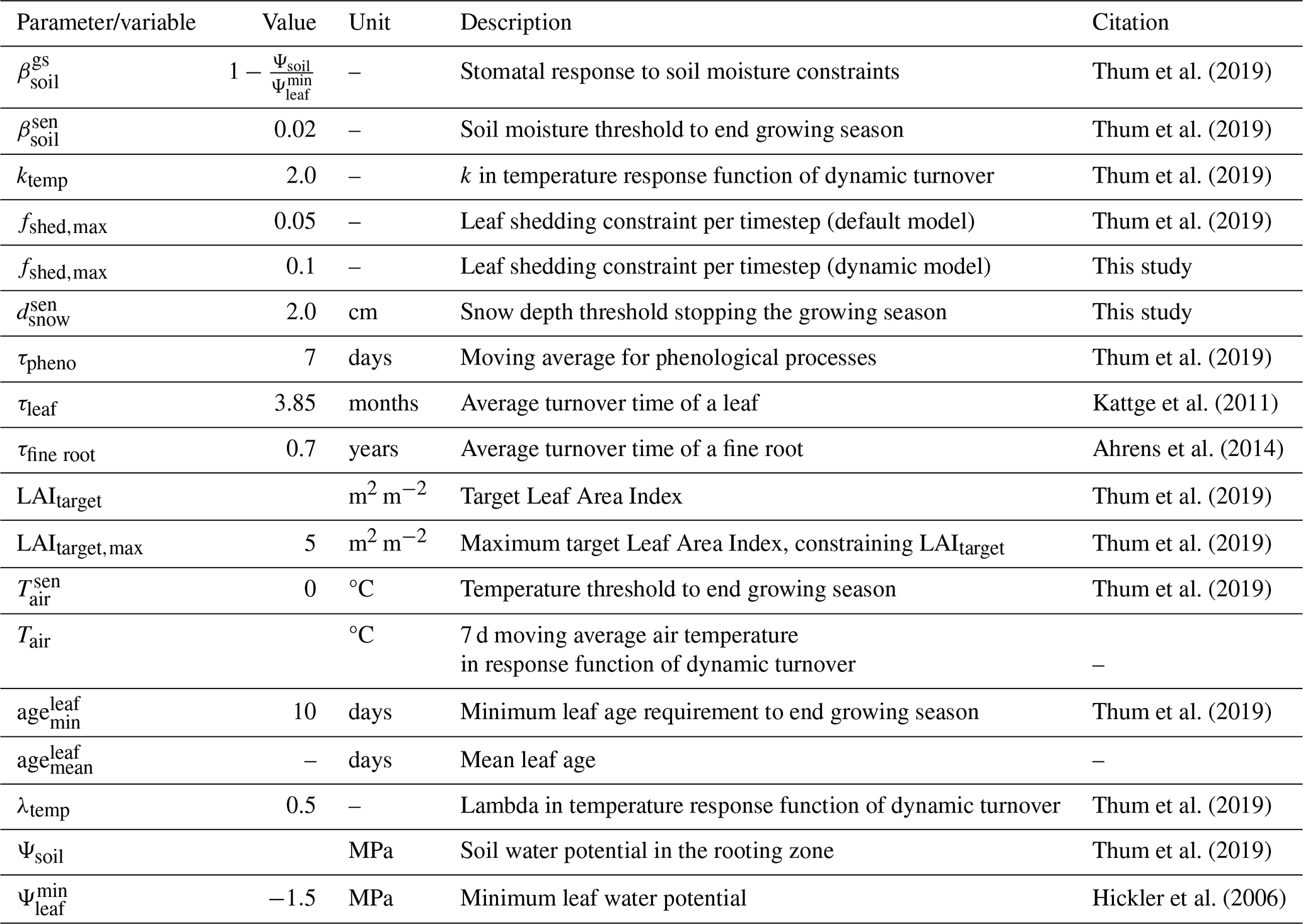
During the growing season, fine roots also turn over continuously (Eq. A4) and this is assumed to be mostly driven by predation on fine roots (Thum et al., 2019). At the end of the growing season, fine roots broadly follow an annual or perennial strategy depending on the climatic conditions at the time of senescence (Poppenwimer et al., 2023). They are either shed or retained over the dormancy period depending on the type of grassland (Eqs. A5–A7). In cold grasslands, i.e., where low temperatures initiated the end of the growing season, fine roots are maintained throughout the dormancy period and in seasonally dry grasslands, i.e., where water stress triggers the end of the growing season, fine roots are shed and then regrown once the growing season starts again. If the end of the growing season is initiated by neither cold nor drought but through a negative carbon balance, roots are also shed (Eqs. A8–A10). Storage pools (labile and reserve) are maintained throughout the unfavorable season.
2.3 Dynamic turnover model
Due to the default models' basic representation of end of season dynamics and building on Yang et al. (2023)'s species-specific drought response model in Australian herbaceous systems, we have developed a new representation of leaf turnover to make QUINCY more dynamic (i.e. decoupled from fixed thresholds) and process based. We have decoupled leaf turnover from the growing season and represent it as a continuous function of air temperature, soil water availability and day length. This allows plant growth to be constrained by multiple environmental factors simultaneously and allows biomass turnover on a more continuous basis, as a more accurate representation of multi-species systems. Additionally, the model formulation also includes co-limitation of multiple factors, either concurrent or at different times of year and importantly allows for leaf abscission during the growing season if conditions become unfavorable.
Turnover in the dynamic model is dictated by three components: temperature, moisture and day length which are shown in Fig. 1. The temperature component (, see Fig. 1a) which has been adapted from QUINCY's temperature control function on the meristem (see Eq. A11) is calculated as:
where λtemp and ktemp are scaling factors (Thum et al., 2019) (see Table 1), and Tair is the air temperature in °C averaged over τphen.
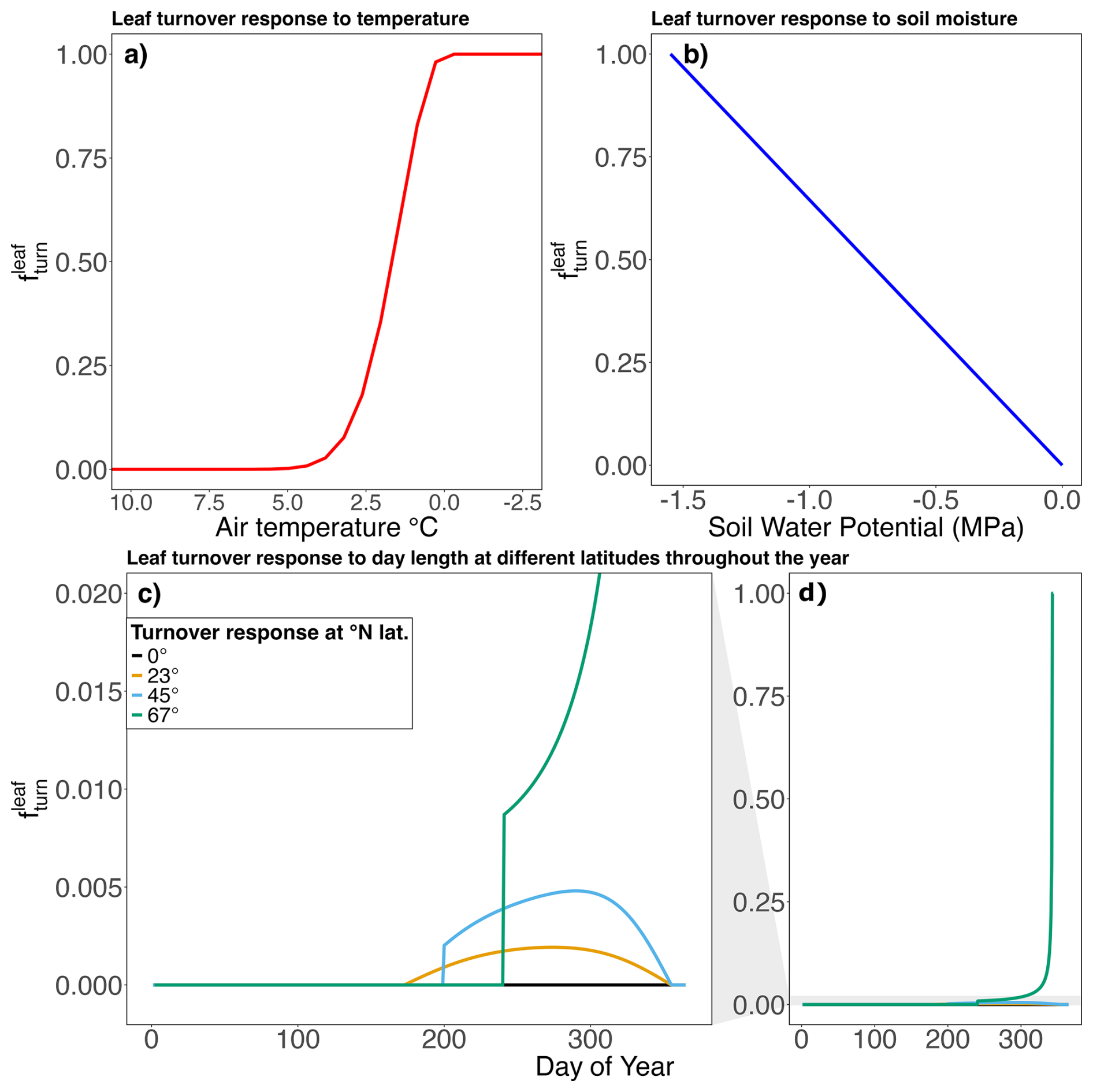
Figure 1The individual impacts of the three environmental stressors: (a) air temperature (see Eq. 6), (b) soil moisture (see Eq. 7), and (c, d) day length (see Eqs. 13–15) on leaf turnover () in the dynamic model (see Sect. 2.3). The combined from these three components is shown in Eq. (16). The leaf turnover response to day length (c, d) is shown for example latitudes on the northern hemisphere, but the model provides continuous global coverage for all latitudes. Panel (d) shows the full range of light induced leaf turnover and panel (c) is an enlarged view of this to show the exact pattern as well as timing of leaf turnover response to changing day length.
The soil moisture stress-induced leaf turnover component of the dynamic model (, Eq. 7) was adapted from the soil moisture constraint function on stomatal conductance (, see Table 1) in QUINCY. With this formulation, leaf turnover increases linearly from its minimum value 0 when soil water potential in the rooting zone (Ψsoil) is 0 MPa to its maximum value 1 at the permanent wilting point (, see Table 1 and Fig. 1b). Ψsoil is defined as the water potential within soil layers where roots are present, weighted by the fraction of roots present in the individual layers. We have opted for a linear relationship between Ψsoil and due to the non-linear relationship between Ψsoil and soil water content (SWC; Θsoil):
where Ψsoil denotes the soil water potential in the rooting zone and the parameter is the minimum leaf water potential (see Table 1) from Thum et al. (2019). The calculations for Ψsoil, which is derived from pedotransfer functions of Saxton and Rawls (2006), and Θsoil can be found in the Supplementary Material (Sect. 6.3) of Thum et al. (2019).
Having a day length component () in the dynamic leaf turnover model is important especially for high-latitude grasslands for two reasons. First, autumn phenology in those regions happens rapidly which can be attributed to the short growth period (∼3 months of snow-free season) and second, light may become a limiting resource for plants toward the end of the growth period (Chapin et al., 2012; Richardson et al., 2012; Tang et al., 2016). We utilize the difference in day length throughout the year to capture the rapid autumn phenology at higher latitudes (Chapin et al., 2012) whilst still retaining a low impact of day length at lower latitudes where phenological events take longer and light may not be a limiting factor. We choose this approach over other more direct measures such as photosynthetic photon flux density (PPFD), because such metrics are strongly influenced by short-term meteorological variability and we wanted to avoid that our model responds to conditions such as prolonged cloud-coverage by shedding leaves at the wrong time of the year. Moreover, when averaged over longer time scales, PPFD exhibits a seasonal pattern that closely aligns with the annual cycle of daylight duration, therefore providing no significant advantages over the simpler day length approach.
Day length (Dn, h), defined as the time between sunrise and sunset, follows the calculations from Cooper (1969) and is calculated from site latitude in degrees (ϕdeg) and solar declination (δdeg, Eq. 8) for a given day of the year (n). ϕdeg and δdeg are converted to radians (Eqs. 9 and 10) to calculate the sunset hour angle (ωs, Eq. 11), which is then used to calculate Dn (Eq. 12).
where , ϕrad and δrad are the site latitude and declination in radians, respectively and h.
To calculate , we use the rate of change in photoperiod, defined as the difference between the current day length (Dn) and the length of the previous day (Dn−1) to shed increasingly more leaves. Because day length is a daily variable, is calculated once per day and remains constant across all half-hourly time steps (dt) within that 24 h period. If day length is increasing (i.e. ) or more than 15 h of day light are available on the current day, is zero (Eq. 13). After the summer solstice, once day length starts to decrease (i.e. ) and less than 15 h of day light are available, we use the difference between Dn−1 and Dn to calculate the rate of change over Dn to shed increasingly more leaves until the maximum rate is reached at the September (March on Southern hemisphere) equinox (Eq. 14). We introduced the 15 h threshold as we assume that above 15 h of day light, light is not limiting. From the equinox the shedding rate decreases again until the winter solstice or when day length reaches zero (polar night, see Eq. 15). The use of solstices and equinoxes follows directly from the geometry of Earth's orbit. The solstices mark the turning points of this cycle where the Sun's declination changes the most slowly at the summer and winter solstices, so daily changes in day length approach zero. At the equinoxes the Sun crosses the celestial equator, where the rate of change of declination is maximal, and therefore the rate of change of day length (i.e. ) is also highest. In summary, the three cases of the light component are calculated as:
if , or Dn>15 h:
if and day length is <15 h:
if polar night (i.e. Dn=0 h):
where Dn is the current day length and Dn−1 is the length of the previous day.
Using this approach, we are able to increase the rate at which leaves are shed in high latitudes, while lower latitudes remain virtually unaffected as the rate of change of day length at lower latitudes is much lower (see Fig. 1c).
The full dynamic leaf turnover () calculation is shown in Eq. (16). We use a multiplicative interaction to represent the compounding effects of temperature (), soil moisture () and day length () components so that under conditions where more than one factor is limiting, leaf turnover is higher than under conditions where only one of the factors is limiting. The maximum turnover rate per timestep is capped through a parameter fshed,max, which prevents shedding of all leaves at once.
where fi are the individual environmental stress-induced turnover functions (, , , Eqs. 6–15) and dt is the length of one timestep.
The parameter fshed,max, which is also part of the default model and prevents grasses from shedding all leaves immediately when the growing season ends, is set to 5 % (0.05) by default. We have kept this parameter in the dynamic model but ran a parameter sensitivity test in QUINCY to optimize fshed,max as 5 % imposes a too slow shedding of leaves under unfavorable conditions. The results of these tests, which we have conducted at the four main sites, reveal that 10 % or a shedding of all leaves over 10 d at the highest shedding rate () is a more suitable value for our model in terms of daily GPP fit to observational data.
Finally, we have added an additional condition () to the growing season in the dynamic model so that an accumulated snow depth of >2 cm stops the growing season. This does not directly impact the dynamic turnover model as it is not controlled by the growing season, but it stops the growth of new tissue under unsuitable conditions and when the turnover rate is already high due to low air temperature.
2.4 Data description
2.4.1 Site description
We selected four main sites for model development and evaluation (Table 2) based on their differing environmental conditions and available data to test model performance at different extremes as well as at moderate environmental conditions, that may be affected by temperature (i.e., low temperatures in winter) as well as soil moisture changes (e.g., dry season). The arctic site was chosen specifically due to its location north of the Arctic circle to test our model under polar day/night conditions.
Nair et al. (2024)Table 2Climate and vegetation information with data used for evaluation and data sources as well as length of available time series at the four selected sites ES-LMa, IE-Dri, US-Tol and CGE. Climate data is calculated from QUINCY atmospheric forcing filtered for the years matching the observational data.
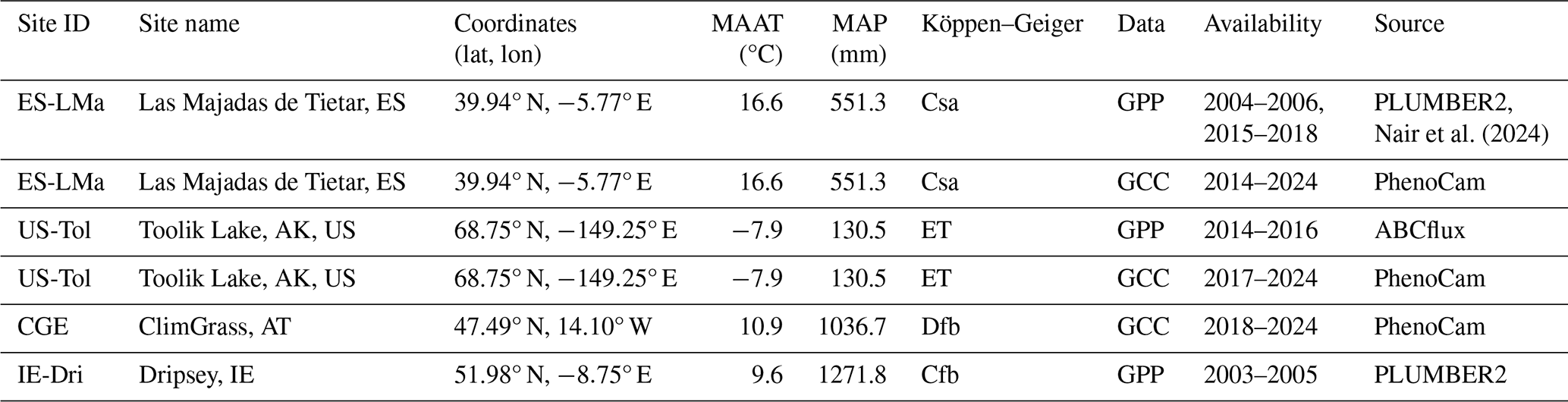
The first site is a seasonally dry “dehesa” site (Köppen–Geiger: Csa), Majadas de Tiétar, Spain (PLUMBER2: ES-LMa; 39°56′24.68′′ N, 5°46′28.70′′ W). The mean annual precipitation (MAP) is 650 mm, the dry season starts in May and lasts until September at which point it starts to rain again and the main rainfall occurs throughout the winter months and spring. The mean annual air temperature (MAAT) is 16.7 °C (Luo et al., 2018). The second site is a seasonally cold montane meadow (MAT: 10.9 °C; MAP: 1036.7 mm, Köppen–Geiger: Dfb) located in the Austrian Alps, the ClimGrass experimental site at the Agricultural Research and Education Centre Raumberg-Gumpenstein, Austria (hereafter CGE). This montane meadow site is managed through biomass harvesting three times a year during the growing season. The site does not have a flux tower. The third site, Toolik Lake (US-Tol) located in the Alaskan tundra (Köppen-Geiger: ET) near Toolik Field Station was selected to test the light-limitation in our dynamic turnover model. The vegetation at the site consists of tussock and wet sedge tundra and the MAAT and MAP at Toolik Lake are −7.9 °C and 130.5 mm, respectively. The fourth site near Dripsey, Ireland (PLUMBER2: IE-Dri), a grassland intensively managed for grazing and silage harvesting (more details in Kiely et al., 2018), does not experience severe dry seasons or cold temperatures and was therefore chosen to test our model under “moderate” conditions (MAAT: 9.6 °C; MAP: 1271.8 mm, Köppen–Geiger: Cfb). The vegetation at Dripsey is classified as grasslands (IGBM: GRA) by the European Fluxes Database Cluster (https://www.europe-fluxdata.eu/, last access: 29 March 2025).
Furthermore, to test global applicability of our model beside the four main sites, we have tested it at a number of sites (Fig. B1) across different climates of the PLUMBER2 dataset (Ukkola et al., 2021). PLUMBER2 is a quality-controlled synthesis of FLUXNET2015, La Thuile and OzFlux flux data from 170 sites, created specifically for evaluating land surface models. For this we have selected all sites classed as short-stature herbaceous vegetation, which results in 56 grassland sites spanning 14 Köppen–Geiger climatic zones that range from unproductive to highly productive grasslands with mean annual GPP of 42.60 to 2596.5 g C m−2 yr −1. For each site the time interval of available data varied and mean annual GPP was calculated from the entire available time intervals per site.
2.4.2 Data used for evaluation
We use Gross Primary Productivity (GPP) data from eddy covariance towers at the three sites ES-LMa, IE-Dri and US-Tol. For ES-LMa data is available from 2004 to 2006 in PLUMBER2 and we also used flux data from 2015 to 2018 for ES-LMa from Nair et al. (2024). For IE-Dri flux data in PLUMBER2 is available from 2002 to 2005. For US-Tol we use GPP data from the FLUXNET site US-ICs (Imnavait Creek Watershed), which is located approximately 10 km east of Toolik Field station. Data is available as FLUXNET community product from 2014–2016 and we aggregated GPP from half-hourly to daily GPP for this site as well. CGE is a miniFACE site so there is no GPP data available for this site. For the PLUMBER2 subset of sites (56 sites), we calculated mean annual GPP for the two models and compared it with observations.
As well as GPP data, we use Green Chromatic Coordinate (GCC) data from PhenoCam images from the PhenoCam network (Seyednasrollah et al., 2019; Richardson et al., 2018) to test our model at ES-LMa, US-Tol and CGE. IE-Dri does not have a PhenoCam camera. GCC data reflects the greenness of the vegetation, and can be used to infer the start and end of the growing season. GCC is calculated from visible light RGB bands (Sonnentag et al., 2012) (see Eq. 17). This helps suppress noise in the data (Richardson et al., 2018). We used the phenocamapi R package (Seyednasrollah, 2018) to obtain the GCC data and the available years for each site are shown in Table 2. We compare the GCC data with model LAI to investigate the timing of leaf senescence. For the purpose of visualizing and comparing seasonal dynamics rather than actual magnitude of LAI compared to GCC, we have normalized predicted LAI and observed GCC relative to the mean annual maximum and minimum value of each metric. LAI, being a metric of leaf area to ground area, is a three dimensional metric, whereas GCC, being derived from images of the canopy, is a two dimensional metric. Keenan et al. (2014) shows that LAI lags behind GCC at high LAI values, since GCC can reach its seasonal peak when leaves are not fully developed and therefore LAI has not reached its peak yet. Similarly, during leaf senescence GCC can decrease earlier than LAI. However, both metrics follow a broadly similar pattern and are able to show seasonal changes to the canopy.
where “DN” are the digital numbers of the red, green and blue channel (RDN, GDN, BDN).
2.4.3 End of season dynamics
To test if we are able to predict the end of the growing season more accurately with our new dynamic model, we estimated and compared end-of-season (EOS) dates for the EC flux data (observed daily GPP) and the default and the dynamic model (predicted daily GPP) using the “phenofit” package (Kong et al., 2022) in R (R Core Team, 2021). We rough fitted the data with a weighted HANTs function (Verhoef, 1996; Yang et al., 2015a). Next, weight updating using the TIMESTAT function (Jönsson and Eklundh, 2004) and finally fine fitting the data using logistic approach “Elmore” (Elmore et al., 2012). EOS dates were then estimated from the resulting smoothed GPP values with the derivative method. Sites where no growing season or multiple growing seasons could be detected were excluded from the analysis resulting in 37 sites. For more information and a detailed overview of these methods refer to Kong et al. (2020, 2022). The estimated EOS dates for the four main sites ES-LMa, CGE, IE-Dri and US-Tol are displayed in Fig. B3.
Since the aim of our model is to improve EOS dynamics, we further use these estimated EOS dates to quantify how well the two models (default and dynamic) fit the period of senescence in EC data. We test how well predicted GPP fits the observed GPP for the period from the calculated EOS date until the first absolute minimum in daily GPP (14 d smoothed) following the EOS date, but before the next growing season starts. We used the overlap of the calculated periods EOSflux−minflux and EOSQ−minQ (flux = EC flux; Q = QUINCY) for the analysis. The start of the growing season is also calculated with the phenofit package using the same setup and we excluded sites with double growing seasons and sites with growing seasons that span multiple years resulting in 32 sites.
All statistical analyses were done in R. For mean absolute error (MAE), root mean square error (RMSE) and normalized RMSE (NRMSE, normalized with observedmax−observedmin) we used the corresponding functions from the hydroGOF package (Zambrano-Bigiarini, 2024). Correlation coefficients were calculated using the method “Pearson” (ρ), adjusted r2 calculated from linear model, F-statistic (df) from ANOVA and p values using TukeyHSD for three pairs of group means. Global Köppen–Geiger climate classes for each site were extracted from raster data with 1 km resolution (Beck et al., 2018).
2.4.4 Model driving data and setup
QUINCY is driven by atmospheric forcing data from site-level measurements. Half-hourly air temperature and precipitation data as well as downward radiation, air pressure, humidity and wind velocity used are from PLUMBER2 (Ukkola et al., 2021) or site level measurements in the case of ES-LMa and CGE. Soil properties in QUINCY are prescribed at site level from the SoilGrids database (Hengl et al., 2017), atmospheric CO2 comes from Le Quéré et al. (2018), N deposition from Lamarque et al. (2010, 2011) and P deposition from Brahney et al. (2015) and Chien et al. (2016). Meteorological forcing data from 1901 until the begining of each site recording period was created with repeated years of available data, and with fully transient CO2 and nutrient deposition. We ran QUINCY with coupled C-N cycling and prescribed P. The model requires a spin-up period to equilibrate vegetation and soil pools, which for the purpose of this study was 500 years with repeated data from 1901–1930, including a spin-up accelerator for slow soil pools. After the spin-up period, simulations for the four main sites start in 1901 and were run until the last year of available meteorological data, which vary per site. For the multi-site analysis, the spin-up length was the same as for the four main sites but the simulations all ran for 124 years (1901–2024). Snow is enabled and fire disturbance was disabled and PFTs are parameterized with data taken from the TRY dataset (Kattge et al., 2011), which is a global dataset of plant traits.
3.1 Site-level seasonality
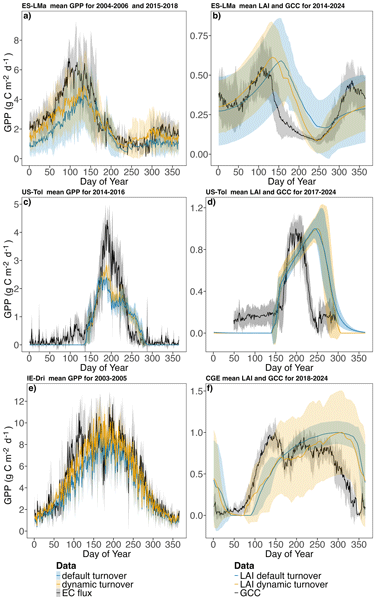
In the seasonally dry grassland, ES-LMa, we are able to reduce the delay of the onset of senescence (Fig. 2b) and the overall seasonal dynamics of modeled GPP (Fig. 2a) fit the EC data better in our dynamic model compared to the default model (adj. r2=0.77 and 0.88, and RMSE 1.25 and 0.76 g C m−2 d−1, respectively, see Table 3). The dynamic turnover improves daily GPP fit in spring and immediately before the dry season, as well as after the dry summer period at the start of the new growing season. This leads to an increase in annual GPP (from default: 481.80±338.143 to dynamic: 613.06±403.52 g C m−2 yr−1, Fig. 3 and Table 4) meaning that the dynamic model's annual GPP is closer to the observed annual GPP (EC) of 729.43±479.62 g C m−2 yr−1, although the default model is not significantly different from the EC data to begin with. Further, there is no detectable significant difference in annual GPP between the default and dynamic model (Table 4). However, overall long-term ecosystem C storage in the dynamic model is higher than in the default model (Fig. 4). The same improvements as in the seasonal GPP dynamics can also be seen in the modeled LAI compared with GCC. We are able to reduce RMSE from 0.17 in the default model to 0.15 in the dynamic model and increase the adj. r2 from 0.10 to 0.39 (Fig. 2b). Although, the seasonal mismatch of LAI and GCC is still quite pronounced in the dynamic model, this is expected due to the comparison of two different metrics.
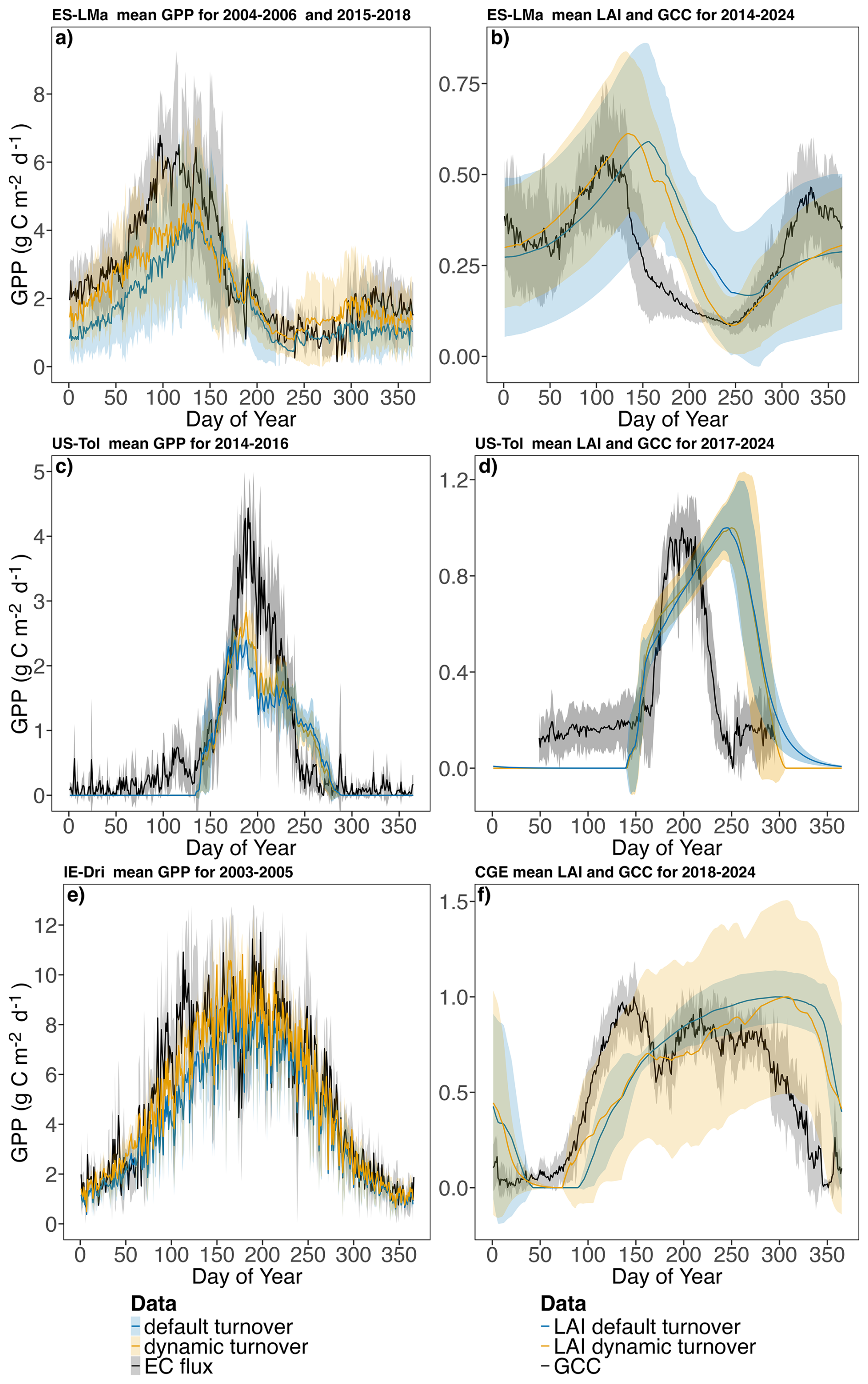
Figure 2Default and dynamic turnover model performance at sites ES-LMa (a), US-Tol (c) and IE-Dri (e) with mean daily GPP and ES-LMa (b), US-Tol (d) and CGE (f) with normalized mean daily LAI and GCC. Shaded areas show one standard deviation.
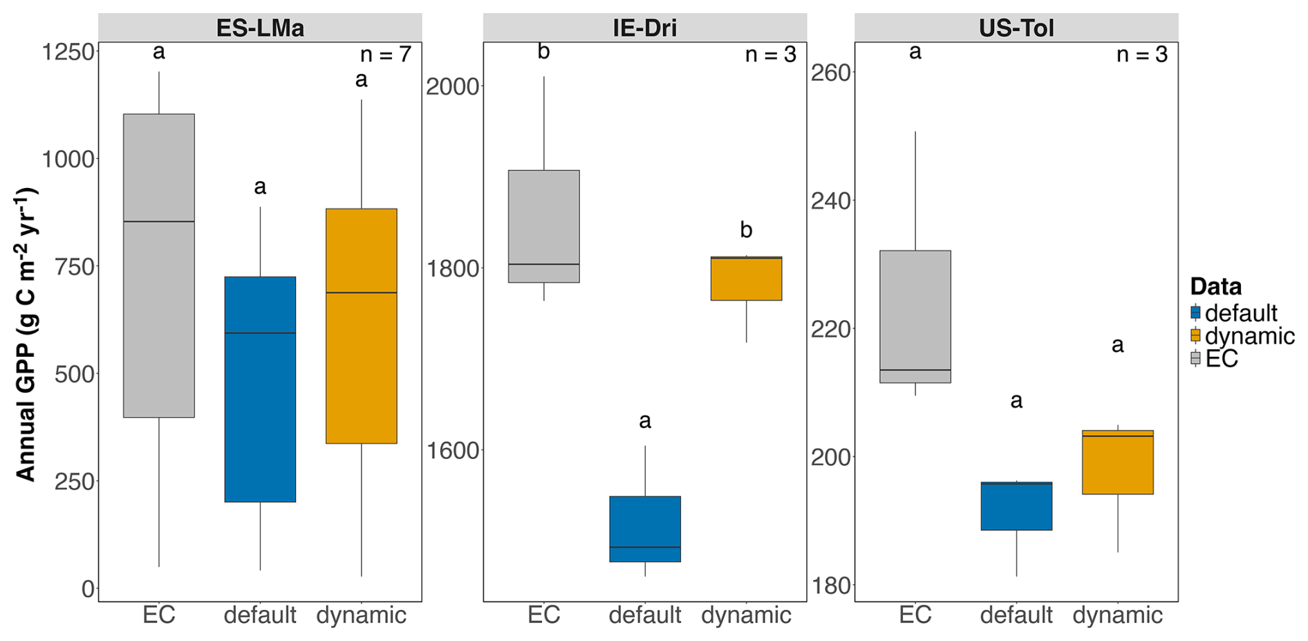
Figure 3Mean annual GPP and 25th- and 75th-percentile for ES-LMa, IE-Dri and US-Tol for the two models (default and dynamic) as well as EC flux data with number of available years of data (n, see Table 2). The displayed simulations for the default and dynamic model matches the time series range of the EC data. Letters above each bar indicate statistical significance (Tukey's p<0.05), where groups sharing the same letter are not significantly different and groups with different letters represent a significant difference between means (for p values see Table 4).
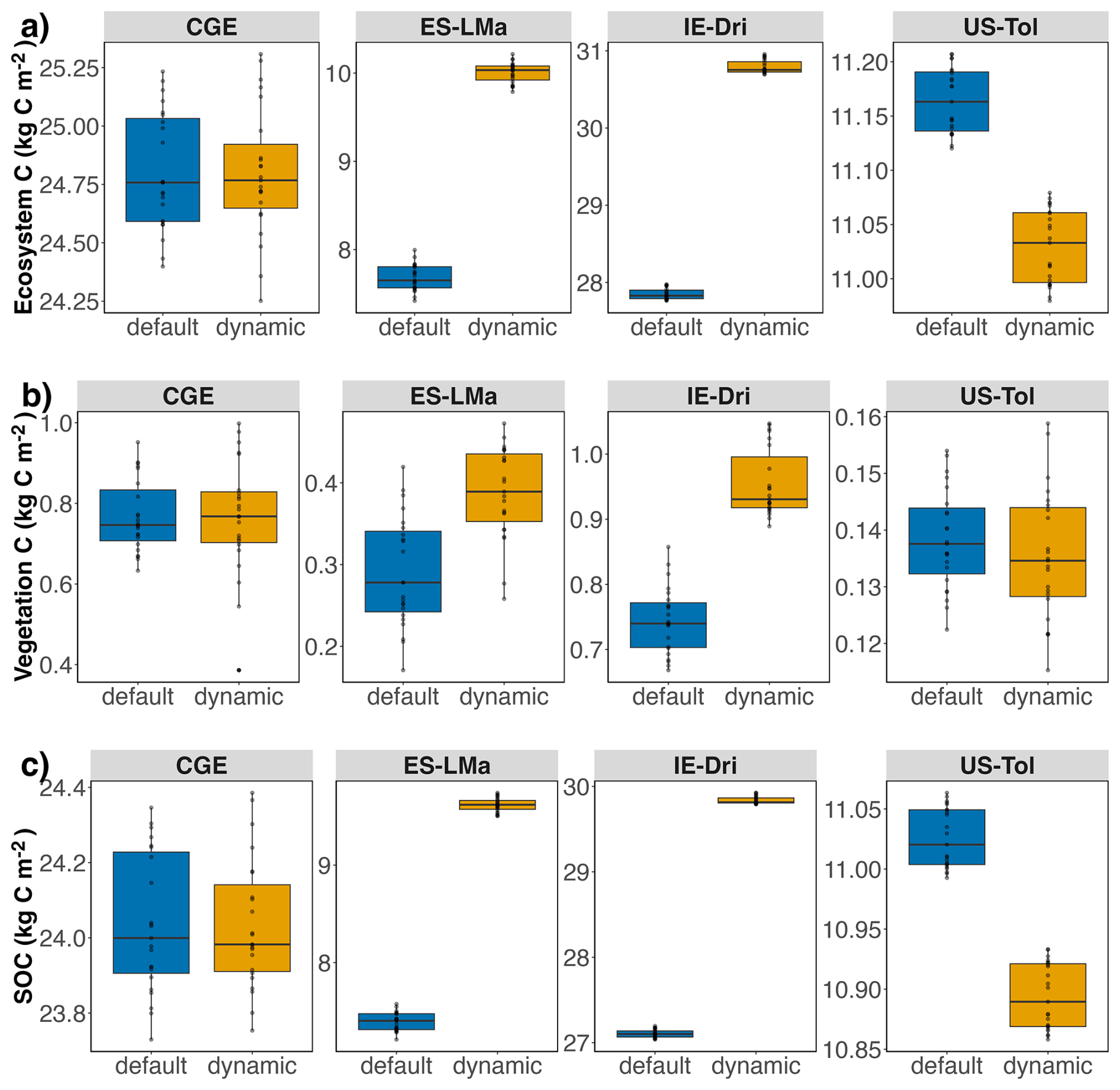
Figure 4Mean annual (a) ecosystem C, (b) vegetation C and (c) soil organic carbon (SOC) of the default model and dynamic model at the four main sites IE-Dri, CGE, ES-LMa and US-Tol for the years 2000–2022. Statistical results are shown in Table C3.
Table 3Default and dynamic turnover model fits (Pearson's ρ and adjusted r2) and errors (MAE, RMSE, NRMSE) against EC flux data at ES-LMa, IE-Dri and US-Tol with mean daily GPP (g C m−2) and ES-LMa, US-Tol and CGE with normalized mean daily LAI compared with normalized PhenoCam GCC.
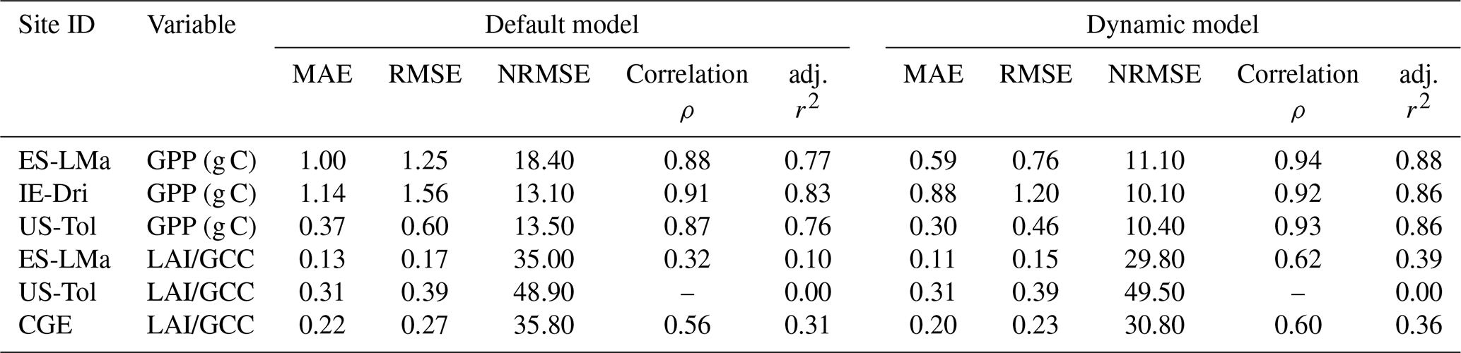
Table 4Mean annual GPP and standard deviation representing inter-annual variation for sites ES-LMa, IE-Dri and US-Tol across the two models and EC flux with number of years of EC flux data (n, see Table 2 for available years), F-statistic (df) from ANOVA as well as p values from TukeyHSD for three pairs of group means.

For the montane, seasonally cool grassland, CGE, where cold winter temperatures are the main determinant of leaf senescence, the default model was unable to capture the onset of winter and showed a delay of nearly 60 d (Fig. 2f). With the direct response to temperature in our dynamic model we are able to shed leaves quicker at the end of the season around November and therefore achieve an overall better fit of predicted LAI to observed GCC (adj. r2 default model: 0.31, dynamic model: 0.36) and we are able to reduce RMSE from 0.27 to 0.23. Leaves also start to grow earlier in spring compared to the default model as shown by an earlier increase in LAI, which brings the start of the season closer to the observed start of the growing season as shown by the GCC data. Long-term C storage however remains unaffected by the dynamic model (Fig. 4 and Table C3).
At the cold and seasonally light-limited site, US-Tol, the default model was unable to reproduce GPP dynamics, especially in the summer, where it underestimated the magnitude of daily and consequently annual GPP (Fig. 3). Similarly to ES-LMa, the dynamic model is able to reduce the error in daily GPP here (Fig. 2c). The RMSE of daily GPP was reduced from 0.60 g C m−2 d−1 in the default model to 0.46 g C m−2 d−1 with the dynamic model (Table 3) and annual GPP increased from 191.10±8.49 in the default model to 204.30±12.72 g C m−2 yr−1, compared to the EC flux annual GPP estimate of 224.57±22.72 g C m−2 yr−1 (Table 4). Although the mean differences exceed the inter-annual standard deviations, the ANOVA indicates that annual GPP of neither model is significantly different from each other nor from the EC flux estimate (p>0.05, Fig. 3 and Table 4), likely reflecting the small sample size (n years=3). The increase, especially in summer daily GPP, also leads to a better model fit of the dynamic model (adj. r2: 0.76 (default) and 0.86 (dynamic)), but LAI still shows an overall poor fit in the dynamic model (adj. r2: 0.0002 (default) and 0.0028 (dynamic)) even though we are able to replicate the steeper drop of GCC better and shift the date of minimum LAI from mid January to early November (Fig. 5d). Just as at the seasonally cold site CGE, long term C storage remains unaffected with negligible decreases in SOC stock (Fig. 4 and Table C3).
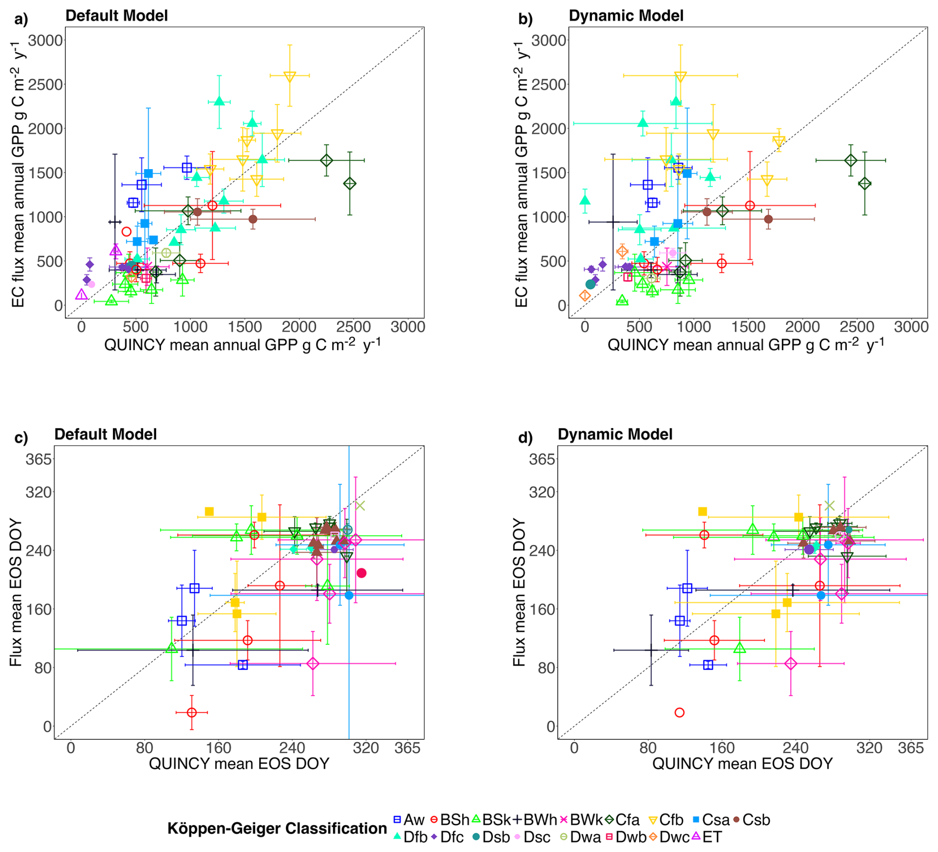
Figure 5Capability of the default and the dynamic turnover model to predict mean annual GPP (a, b) compared to observed EC flux mean annual GPP (g C m−2 yr−1) at 56 sites (see Table C2) as well as mean EOS dates (c, d) at 37 sites (see Table 5) of the default and the dynamic model and compared with EC flux EOS dates. EOS dates were calculated from daily GPP using “phenofit” package (Kong et al., 2022). The number of sites is lower in the panel (c) and (d) due to the exclusion of sites with dual growing seasons or where no EOS could be detected. This is documented in detail in Sect. 2.4.3. Error bars are 1 SD representing inter-annual variation and the colors and point shapes represent Köppen-Geiger climate zones. The climate zones displayed are: Aw: Tropical Savanna, As: Tropical Dry Summer, BSh: Hot Semi-Arid, BSk: Cold Semi-Arid, BWh: Hot Desert, BWk: Cold Desert, Cfa: Humid Subtropical, Cfr: Temperate Fully Humid Warm Summer, Csa: Hot-Summer Mediterranean, Csb: Warm-Summer Mediterranean, Dfb: Humid Continental Warm Summer, Dfc: Subarctic Cold Summer, Dwa: Continental Dry Winter Hot Summer, Dwb: Continental Dry Winter Warm Summer, Dwc: Continental Dry Winter Cold Summer, ET: Tundra.
At IE-Dri, a site that is neither driven by strong temperature nor moisture fluctuations or extremes, with a more continuous growing season and turnover, the dynamic model performs very well (Fig. 2e), as the capacity for continuous turnover is a key new factor in the model. The main drivers of leaf turnover at IE-Dri are soil moisture and day length, though their overall contributions remain small (Fig. B2). With the dynamic model, we can capture the seasonal GPP fluctuations and its amplitude accurately and we reduce the RMSE of daily GPP from 1.56 in the default model to 1.20 in the dynamic model and increase the fit from 0.83 to 0.86 (adj. r2) compared to daily EC flux GPP (Table 3). This also leads to a significant increase in annual GPP from the default model with 1519.36±75.43 to 1780.66±54.45 g C m−2 yr−1 in the dynamic model (p=0.03, Fig. 3 and Table 4) and annual GPP, which in the default model differed significantly (p=0.01, Table 4) from the observed EC annual GPP (1859.25±132.35 g C m−2 yr−1), shows no significant difference in the dynamic model (p=0.59). This also influences long-term C storage, where the dynamic model shows a significantly higher C stock in soil and vegetation (Fig. 4 and Table C3).
Overall, we are able to improve the response of grasses to seasonal moisture, cold and light limitation across all four main sites. We are able to reduce error and improve model fit in predicting seasonal trends of GPP and LAI (Fig. 2 and Table 3), which lead to improves annual GPP estimates (Fig. 3 and Table 4) resulting in significant differences in long term soil C storage (Fig. 4 and Table C3).
3.2 Multi-site comparison
We tested the performance of our dynamic model at 56 sites across climate zones. We tested the whole season fit using mean annual GPP (Fig. 5a and b and Table C2), our models' capability to predict the onset of senescence using end of season date for the same sites (Fig. 5c and d and Table 5), as well as end of season fit, i.e., the senescence period between the end of season date to the first following minimum GPP, before the next growing seasons starts (Fig. 6 and Table 6).
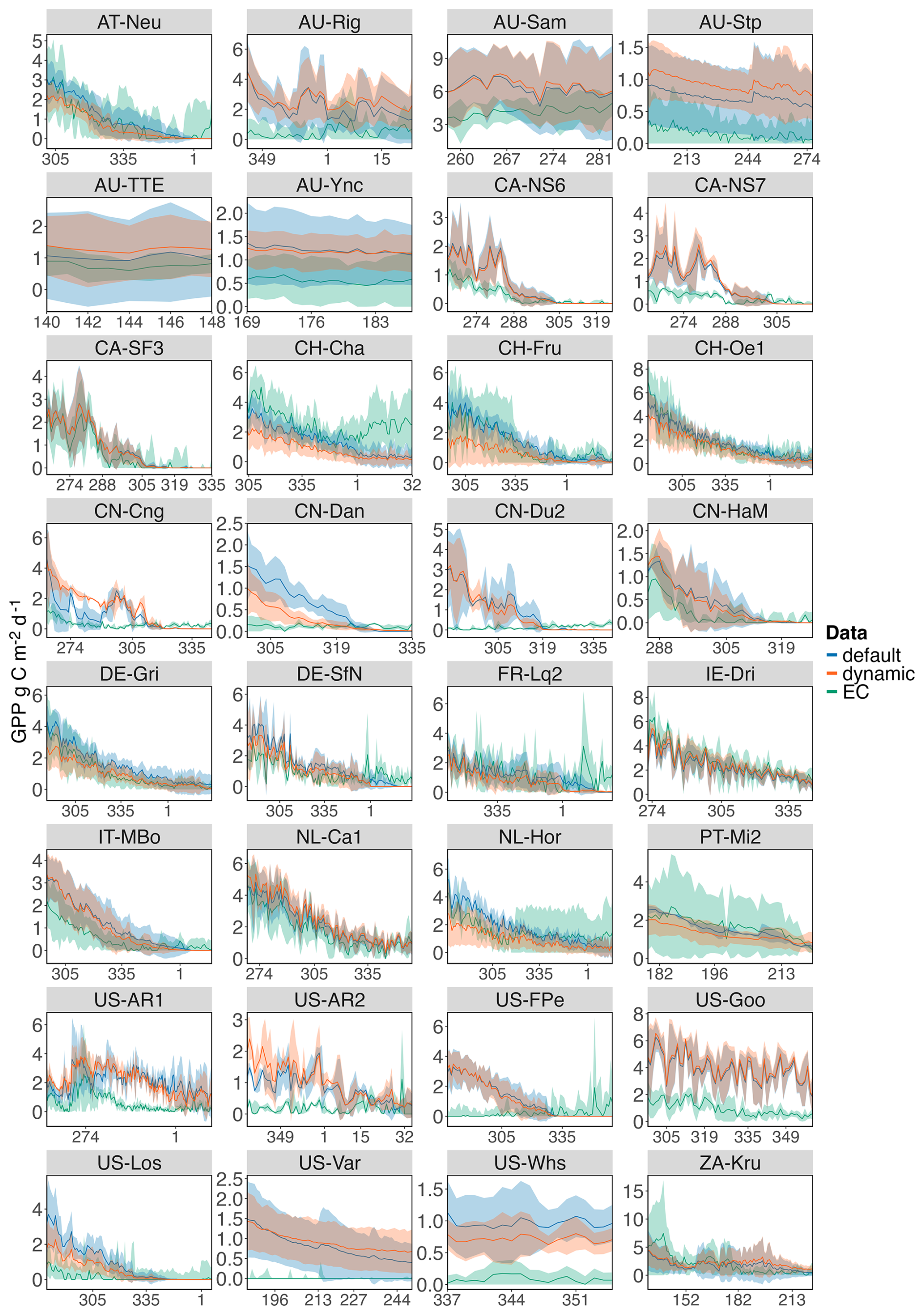
Figure 6End of season (EOS) fit of modeled mean daily GPP (g C m−2 d−1; blue: default and orange: dynamic model) and flux tower mean daily GPP (g C m−2 d−1; green) at 32 PLUMBER2 sites (for explanation of site IDs see Ukkola et al., 2021). The EOS period displayed for each data source is defined as the period between the calculated mean EOS date (see Table 6) and the first mean minimum GPP date following it and for comparison the overlap of all end of season periods (EC flux, default and dynamic model) is used here. The shaded areas represent 1 SD. The EOS dates are calculated using “phenofit” package (Kong et al., 2022) and only sites with one EOS date per year have been selected.
Table 5Mean EOS dates (“Mean EOS”) of EC data, default and dynamic model for 13 different Köppen–Geiger climate classes (“KG class”; 37 sites in total) shown in Fig. 5c and d as well as associated errors (in days; MAE, RMSE, NRMSE) between EC data and default model and between EC data and dynamic model. “n sites” indicates the number of sites within each climate class.
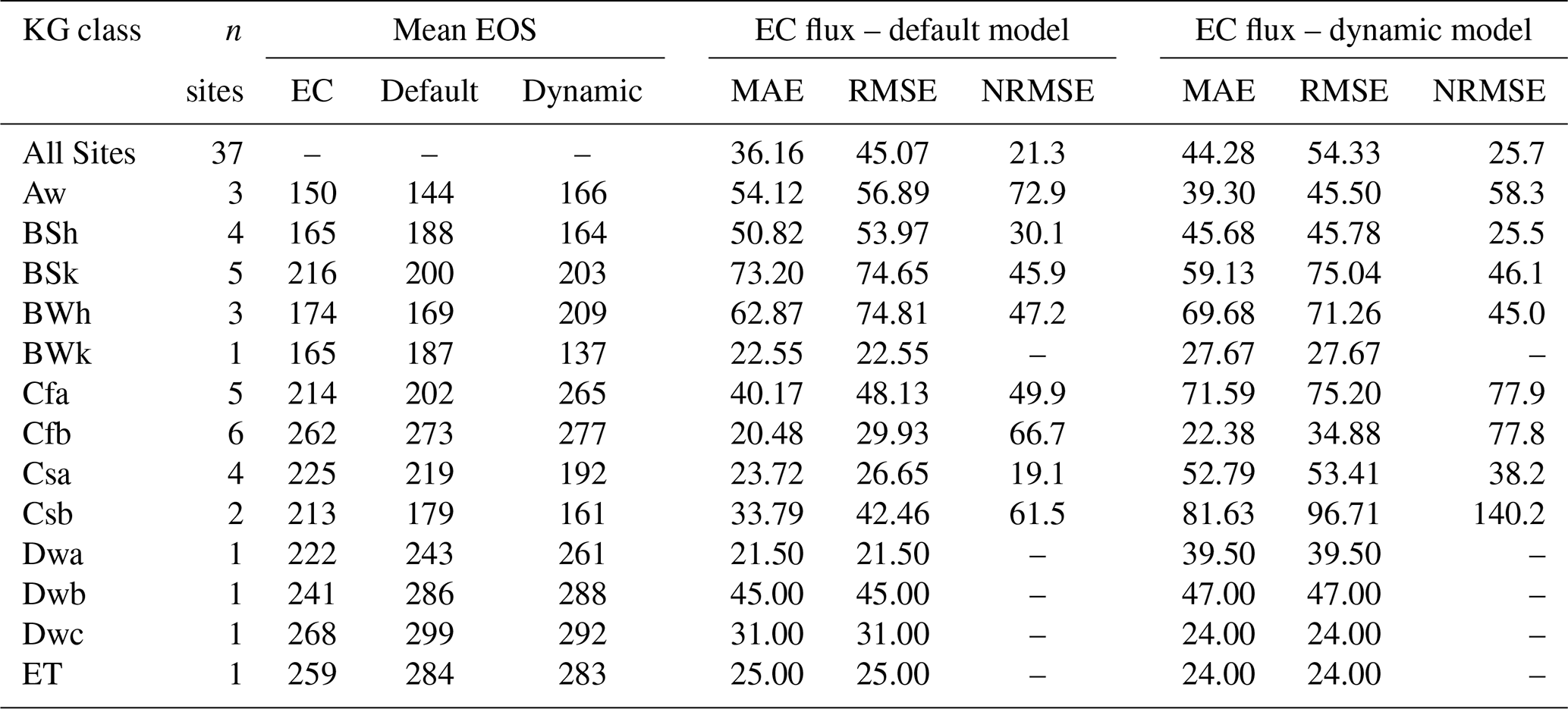
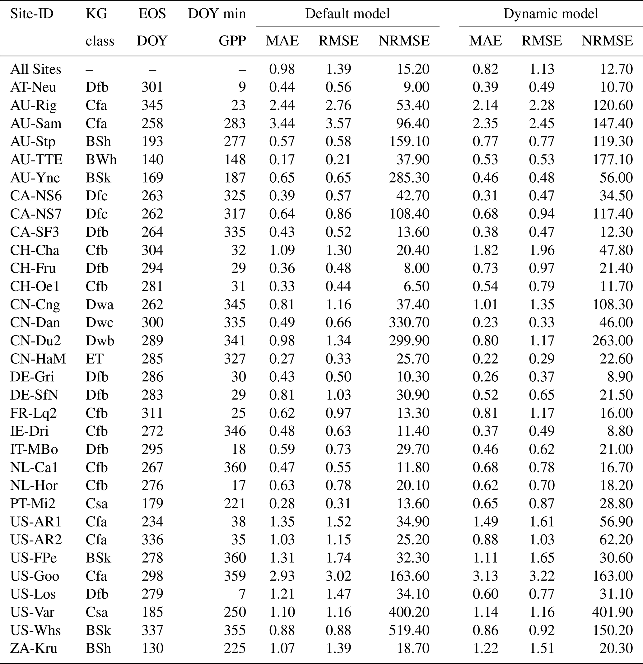
Table 6Model error of the senescence periods shown in Fig. 6 for 32 PLUMBER2 sites and 12 Köppen–Geiger climate classes (“KG class”). The shared senescence period from “EOS DOY” to “DOY min GPP” is the overlap of the end of season periods of all three data sources (EC flux, default and dynamic model). For each data source the end of season period is determined as the time between calculated EOS date and day of the year when GPP reaches its minimum following this EOS date. EOS DOY and DOY min GPP are averaged over available site years. The Mean Absolute Error (MAE), Root Mean Square Error (RMSE) and Normalized Root Mean Square Error (NRMSE) describe the model fit of the senescence period. At sites where the mean minimum GPP date is smaller than the corresponding EOS date (e.g., AT-Neu), the senescence period spans across into the new year.
Over all sites, both the default and dynamic models have similar model fits (Table 5), however, the dynamic model performs better in several key areas. The default model consistently underestimates annual GPP at tropical savanna and hot summer Mediterranean sites (Aw: 665.00 (default) vs. 1358.00 (EC), n site years = 17; Csa: 592.00 (default) vs. 967.00 g C m−2 yr−1 (EC), n site years = 21), while overestimating GPP in both hot and cold semi-arid sites (BSh: 731.00 (default) vs. 661.00 (EC), n site years = 20; BSk: 522.00 (default) vs. 210.00 g C m−2 yr−1 (EC), n site years = 36). The dynamic model improves model fit at tropical savanna sites (RMSE default: 698.86 and dynamic: 681.06), although the GPP remains low (dynamic: 685.00 g C m−2 yr−1), and the dynamic model shows a significant improvement at Mediterranean sites (RMSE default: 482.72 and dynamic: 315.81). Model GPP at subarctic and tundra sites is also improved by the dynamic turnover (ET: 358.00 (EC), 157.00 (default), 171.00 g C m−2 yr−1 (dynamic) and RMSE: 220.77 (default) vs. 202.24 (dynamic, n site years = 16); Dwc: 318.00 (EC), 358.00 (default), 393.00 g C m−2 yr−1 (dynamic), n site years = 2).
The model performance in predicting EOS dates (Fig. 5c and d and Table 5) follows a pattern similar to the annual GPP results, except that Csa sites perform worse in the dynamic model (RMSE: 26.65 (default) and 52.41 d (dynamic)) and BSh (hot semi-arid) and BWh (hot desert climate) show reduced errors. Overall, the model shows improved RMSE of EOS dates at 12 out of 37 sites. The dynamic model performs better again at Aw, Dwc and ET sites compared to the default model. At tropical savanna (Aw) sites the dynamic model overestimates the EOS date compared to EC flux data where the end of the season is on DOY 150. The dynamic model EOS is 166 and the default model is 144. However, the dynamic model shows a lower RMSE of 45.50 d compared with the default model where RMSE is 56.89 d (n sites = 3). At hot semi-arid sites (BSh) the dynamic model shows a significant improvement over the default model with a near perfect match of EOS DOY (EC: 165, default: 188, dynamic: 164) and RMSE reduces from 53.97 to 45.78 d (n sites = 4). Hot desert sites (BWh) on the other hand, show a reduced RMSE from 74.81 (default) to 71.26 d (dynamic, n sites = 3) but similarly to tropical savanna sites, place the EOS date later in the year (EC: 174, default: 169, dynamic: 209). At subarctic sites, the EOS is a week earlier in the dynamic model, moving it closer to the EC EOS (EC: 268, default: 299, dynamic: 292) and has a reduced RMSE (default: 31.00, dynamic: 24.00). At the tundra site the dynamic model shows a similar trend but only a fractional improvement of one day (EOS EC: 259, default: 284, dynamic: 283) which results in a marginally improved RMSE (default: 25.00, dynamic: 24.00).
The final analysis in which we separated leaf senescence from the rest of the year to quantify site level end of season fit of daily GPP (Fig. 6 and Table 6) reveals that the dynamic model overall performs better across the 32 sites in terms of error (RMSE default: 1.39 g C m−2 d−1, dynamic: 1.13 g C m−2 d−1). The dynamic model shows a better fit at 17 of the sites (lower RMSE) which span across a wide range of climates, from cold-winter, semi-arid (BSk: n sites = 2), over oceanic (Cfb: n=2), humid-continental (Dfb: n=6; Dwb: n=1) and humid subtropical (Cfa: n=3) to dry-winter (Dwc: n=1), subarctic (Dfc: n=1) and tundra climates (ET; n=1). At hot semi-arid (BSh: n=2), but also some oceanic (Cfb: n=4) and some humid subtropical (Cfa: n=2), hot-summer Mediterranean (Csa: n=2) and continental (Dfb, Dfc and Dwb; n=1 each) sites the dynamic model perform less well. Generally, the fit of senescence periods is better at sites where the dynamic model struggled to estimate annual GPP and EOS date. The extracted periods represent the overlap between the individual EOS periods of EC data and the two models, so it is decoupled from the actual EOS dates, since it is difficult to evaluate the significance of calculating singular dates, which change based on the method used, it may be more important to look at the entire senescence period.
In this study, we present a new dynamic leaf turnover model that is applicable globally in grasslands as implemented in the QUINCY model. Our results show that grasses are able to respond more accurately to environmental conditions by directly controlling leaf shedding with meteorological conditions continuously and interactively. At four sites of differing climate we demonstrate how improving end of season phenology has implications for seasonal carbon dynamics, LAI and annual GPP as well as long term C storage. On a global scale, we show that our new model is able to reduce biases in the senescence period model fit, and again, annual GPP across a wide range of climate zones while also highlighting its shortcomings and the need for a refined model that can account for plant adaptations to their environment and the consequently differing responses to unfavourable growing conditions.
4.1 Beyond temperature response end of season thresholds
Traditional leaf phenology research often focused on mid-latitude temperate systems, where a temperature threshold for both start of season and end of season may be a good approximation, but even in those ecosystems, the modelling focus has been largely on start of season phenology, with end of season processes being much more poorly understood. While progress has been made in stand-alone phenology models (Lang et al., 2019; Yang et al., 2023), implementation in LSMs has been slow (Richardson et al., 2012) and mainly focused on trees and shrubs (Chen et al., 2024). Many models, including LPJ-GUESS (Sitch et al., 2003) and CLM5 (Lawrence et al., 2019), have integrated similar multi-factor phenology models, yet they often rely on discrete environmental triggers. For instance, CLM5 simulates leaf senescence of grasslands through accumulated stress based on moisture, temperature, and day length thresholds. Once these predefined thresholds are surpassed, senescence is triggered. Similarly, LPJ-GUESS utilizes survival fractions of leaves based on climatic conditions and sheds all leaves on the statistically coldest day of the year, therefore introducing a hard-coded threshold for grasses. These discrete, trigger-based mechanisms often fail to capture how ecosystems respond to environmental stress.
Grasslands may be one of the most moisture-sensitive ecosystems on the planet (Cherwin and Knapp, 2012) and drought frequency and intensity is expected to increase with climate change (Spinoni et al., 2018). Yet, models are not able to reproduce observed drought responses of grasslands (De Kauwe et al., 2017), even though the timing of these events has implications on C fluxes (Felton and Goldsmith, 2023) and the capability of shifting grasslands from a C sink to a source (Zhang et al., 2020). To address these limitations, our new dynamic model moves away from binary triggers, allowing us to capture the seasonal drought response in a dehesa, savanna-like, ecosystem, ES-LMa, more accurately and show that controlling senescence as a continuous process rather than a classical threshold end of season can lead to better whole-season model performance. Arid and semi-arid grasslands are frequently composed of species with a variety of levels of drought resistance and a threshold approach can be unsuitable, therefore having a dynamic response to changes in soil moisture conditions can be more ecologically relevant. We show that improving end of season phenology impacts the whole year by alleviating constraints placed on early season growth in threshold models (here: after the dry summer at ES-LMa), which leads to higher early season growth and a better fit with the EC data. Further, more accurate leaf senescence can reduce carbon costs in plants as maintaining leaves requires carbon allocation to respiration. Importantly, we show that improving leaf turnover does not only affect seasonal dynamics, but impacts long term C storage, as well (Fig. 4), where our dynamic model shows significantly higher C storage in the entire ecosystem.
Photosynthetic activity is primarily limited by light and even more so in high latitude ecosystems. At present, light limitation may not be very relevant at high latitudes as snowfall occurs before day length becomes very limiting, but under future climate which will shift the snow-free period later into the year (Myers‐Smith et al., 2019), light limitation may become increasingly important (Lang et al., 2019; Richardson et al., 2012; Tang et al., 2016). This also applies to spring phenology, where earlier snow melt and higher spring temperatures may be able to extend the growing season, however plants may not be able to take advantage of this extended growing season as the short photoperiod very early in the year becomes limiting (Chapin et al., 2012). Our model could predict high latitude grasslands more accurately and give evidence for the importance of day length control in leaf turnover (Ren et al., 2019, 2022; Sakuraba, 2021). Our dynamic model is able to reproduce the end of the season better at US-Tol and to a certain extend improves the peak GPP in the summer at this site (Fig. 2c and Table 3). However, peak GPP in the dynamic model is still underestimated compared to observations, similarly to other tundra sites (Table C2). This is likely due to the model's shortcomings in representing nutrient availability in high-latitudes, an issue common across LSMs (Kou-Giesbrecht et al., 2023).
Continental climates are characterized by seasonal temperature variations and temperature is one of the main drivers for autumn phenology in grasslands (Ren et al., 2022). Higher temperatures in autumn have been shown to delay the onset of leaf senescence in herbaceous plants (Jeong et al., 2011) and climate change is predicted to prolong the growing season later into the year (Arndt et al., 2019), so it is important for models to accurately predict autumn phenology and dynamically respond to changes in temperature. Our dynamic model is able to predict the onset of senescence at CGE better than the default threshold model and is able to reproduce the observed “brown-down” in the GCC better (Fig. 2f). Even at more extreme cold sites such as the tundra site US-Tol, we were able to improve the end of the season and shift the minimum LAI forward by 60 d and closer to the observed minimum GCC. Yet, LAI lags behind the GCC data at both sites in regard to timing of its peak and end of season, but this is expected and consistent with other observations (Keenan et al., 2014; Bórnez et al., 2020). Since GCC is the green fraction of an image taken of the canopy from above and LAI is a measure of leaf area per ground area, the optical greenness of the upper canopy may begin to decline while significant leaf biomass remains, causing a lag in the data compared to actual leaf biomass. This discrepancy is further compounded by snow cover as GCC is highly sensitive to the high albedo of snow, which obscures leaves that may still be physically present and accounted for in the LAI data. However, since GPP at US-Tol also shows a lagged response in autumn phenology, we can assume that the mismatch in GCC and LAI can not solely be contributed to them being different metrics. This lag in GPP is very likely not caused by issues with the dynamic leaf turnover representation alone, but rather leaf growth in QUINCY, as the growing season at US-Tol on average ends only at 280 (see Fig. B3) at which point GPP is already near zero in the EC flux data. Decoupling leaf growth from the growing season, which is also based on a threshold approach may solve this issue. Further, CGE is a managed grassland subject to regular mowing and we did not include a mowing scheme into our model. This leads to sharp drops in greenness after each mowing event, which is lacking in our model (Joseph et al., 2025). This likely at least partly contributed to this mismatch of GCC and LAI apart from them being two different metrics. Finally, our model is also able to improve whole season fit of GPP even at sites that do not experience (severe) cold nor dry periods throughout the year, such as we have shown at the site IE-Dri. The gradual shedding of leaves which is required to replicate these moderate conditions, is only achievable with our flexible approach and the default threshold model which essentially applies the same shedding rate in all climates, cannot reproduce this. As a result we are able to significantly improve annual GPP, match observed GPP closely and show that improving end of season dynamics strongly impacts annual GPP predictions as well as long-term C storage (Fig. 4), which contributes to reducing uncertainties present in global carbon budgets (Bai and Cotrufo, 2022).
4.2 Model flexibility and generality
Our model does not prescribe a priori which of the three triggers is limiting and we show that the model is widely applicable at sites across the globe. It provides a first step towards more flexible, physiology-driven leaf turnover but highlights the need for a more adaptable drought model that is able to incorporate different drought responses such as presented in Yang et al. (2023). The model is able to capture end of season phenology more accurately across a wide range of climates (see Fig. 6 and Table 6). A poorer model fit at some of the sites with the dynamic model is likely caused by knock-on effects from changes in growing season length on new growth at the start of season. The default turnover model may get things right for the wrong reason and may have been able to “mask” delayed start of season as it frequently allowed for very long growing seasons which do not match site observations from EC data, and therefore in terms of carbon budgets (e.g., annual GPP). Furthermore, the dynamic model allows for leaf turnover during the entire growing season which may further impact early season growth by inducing leaf senescence of young leaves if conditions become harsher. This is a more appropriate response and is able to capture events such as late frost in spring that damages leaves, but the default model which effectively removed leaf turnover during the growing season was not able to capture this and therefore placed less pressure on the already underestimated early season growth in QUINCY.
Our model performs well in terms of annual GPP at sites with strong seasonality of precipitation (Aw: tropical savanna and Csa: hot summer Mediterranean) and also temperature (winter-dry subarctic and tundra, Table C2). This demonstrates that our model successfully captures leaf senescence under pronounced seasonal extremes in both moisture and temperature. However, at a number of seasonally cold sites the dynamic model (temperate/continental) shows a worse fit. This may suggest that the model's single temperature response function may not sufficiently account for local thermal adaptation (Körner, 2016), leading to reduced sensitivity in temperate regions with less severe winters. Plants in seasonally cold sites may also lack photoperiodic signaling which triggers senescence through gene expression (Sakuraba, 2021) whereas our model primarily accounts for light limitation. The subarctic (Dwc) site is CN-Dan located at 30.49° N, the subarctic climate of the site is therefore a result of altitude rather than latitude. This suggests that day length turnover in the model has a near zero impact at CN-Dan and the same goes for the second tundra (ET) site, CN-HaM, at 37.37° N. Since the model performs better at these two sites and the sites are located at mid-latitude like the temperate/continental sites that perform worse in the model with the only difference being altitude, it could point toward a lacking temperature sensitivity to cold-hardiness, not a lack of day length control for the worse model fit at continental/temperate sites. Further, models often lack proper representation of constraints on photosynthesis at mid-latitudes which can influence annual GPP, such as the suppressing of photosynthetic activity by low temperature which may contribute to the poor model fit at these sites (Luo et al., 2023; Mäkelä et al., 2004, 2008).
Autumn phenology and its timing (Dragoni et al., 2011; Hollinger et al., 2004; Richardson et al., 2010) is a key part of ecosystem functioning and has been shown to play an important role in predicting net ecosystem productivity (Wu et al., 2013). The dynamic model improves the accuracy of the timing of leaf senescence at subarctic (Dwc) and tundra sites (ET), but not at temperate sites (C climates). Thus, further showing that the model as is parameterized now may be more appropriate for harsher climates and less so for temperate sites. Although, the number of sites with ET and Dwc climate is very low (between one and two sites per class and metric) which reduces confidence in these results, those sites as well as the tundra site US-Tol consistently perform better in terms of errors across all three metrics that we have tested (annual GPP, EOS date and EOS period). Beside the Dwc and ET sites, the model performs better at tropical savanna sites (Aw), and unlike annual GPP, at hot semi-arid and desert sites (BSh and BWh). However, at hot summer Mediterranean sites (Csa), where the end of season is in the summer months caused by a lack of precipitation, the model performs less well. It should be noted that ES-LMa (Csa) is not part of this analysis. At Csa sites, the estimated EOS date in the dynamic model is day 192 (default: 219). This is earlier than the estimated EOS date of the EC data (DOY 225). This indicates that our model, may be overly moisture-sensitive in ecosystems that are defined by dry summers. Yet at tropical savannas, ecosystems that are also characterized by strong seasonal rain patterns and at hot semi-arid and desert sites the model has improved. This highlights that grasslands have vastly different responses to dry conditions and may suggest that a singular drought-response mechanism may not be sufficient and implementing different drought sensitivities, similar to Yang et al. (2023) could improve model performance.
The mismatch in moisture sensitivity is also reflected when extracting the senescence period from the whole year, where our model performs well at sites that do not have a dry season (12 of 18 sites with climate Cfa, Cfb, Dfb, Dfc; indicated by second letter “f”) and it performs less well at sites that are either summer- (second letter “s”) or winter-dry (second letter “w”), with the exception of two cold, semi-arid sites (BSk), one hemi-boreal site (CN-Du2) and one winter-dry subarctic site (Dwc, site CN-Dan). However, Yang et al. (2015b) finds that temperature rather than precipitation is the main driver for autumn phenology in Chinese herbaceous species, which could explain why the model performed better at CN-Du2 and CN-Dan even though seasonally dry sites generally show a weaker fit in our model. Furthermore, at US-Whs, one of the two summer-dry BSk sites located at a relatively high elevation (1380 m a.s.l.), leaf turnover appears to be driven primarily by temperature rather than moisture, which may explain the better model performance there. The generally better fit at mesic sites, as well subarctic/tundra sites could indicate that our model may struggle to reproduce species-specific water-stress adaptations.
Overall the model allows for interaction between triggers and co-limitation, which works well in terms of end of season fit at subarctic sites and temperate/continental sites in central Europe, systems which experience both temperature and light-limitation in both reality and the model. However, other sites in similar climates perform less well, showing the existing uncertainty and high site-specificity of which factor is more important in a co-limitation ecosystem (Estiarte and Peñuelas, 2015). We show that the model is suitable for many herbaceous ecosystems with differing climatic conditions across the globe but its varying performance across similar ecosystems further shows that species- and site-specific adaptations to environmental conditions bring a high uncertainty into modelling grassland leaf turnover and may call for more adaptable responses. Still, our model provides a first step away from threshold-controls in LSMs and towards more process-based models.
Under future conditions where sites may move into more seasonally dry regimes, the dynamic turnover representation may be more adaptable than the previous threshold approach and it consistently performs better at simulating tropical savanna systems. Further, day length provides a hard threshold even as the climate gets warmer and many studies show that plants use it as signaling to induce leaf senescence (Sakuraba, 2021; Lang et al., 2019; Ren et al., 2022). With the incorporation of day length, we can simulate future subarctic and tundra ecosystems better than the previous threshold model which often predicted very long growing seasons well into the light-limited winter, such as we have shown at US-Tol.
4.3 Limitations and future directions
All herbaceous plants share the same leaf turnover in QUINCY and there is no current representation of different life strategies. To improve our current model, the triggers for leaf senescence in herbaceous plants across different climates need further attention, even though efforts over the last decade have been made to close this gap (Lang et al., 2019), but most studies only focus on single sites or species so that there is limited understanding of how day length, temperature and precipitation jointly determine leaf senescence across the globe. Even if this gap is slowly being filled, it will be very difficult to capture differing responses to seasonality caused by differences on a species-level with ecosystem scale data. Our continuous model is a first step towards addressing this issue, however, we also show that this needs further attention in the form of site-specific responses based on climate under the assumption that plants are adapted to the environment they grow in (Körner, 2016). Further, limited data availability for some of the sites introduced uncertainty into our results and reduced statistical power. A limited number of continuous data spanning multiple years combined with the frequency of extreme events over the last decades complicates the development of a general model for leaf turnover. Finally, many grasslands are intensively managed systems, which we do not consider in this study. Management of grasslands, through grazing, harvesting or fertiliser use, has a variety of implications for ecosystem functioning and since we do not consider them in our model, but compare it to EC data from these managed systems, our results were likely impacted by this as well.
The difference in performance between site-level evaluations (Table 6) and climate-level aggregations (Table 5) likely reflects the inherent challenge of representing diverse ecological strategies with a single parameterization. Potential future directions include the incorporation of a drought response parameter based on site level climatological and soil hydrological conditions, to represent local adaptation, so that sites with little soil moisture and temperature fluctuations would show a stronger drought response than seasonally cold or dry and (semi-) arid systems which are more adapted to these conditions. Currently fshedmax ensures shedding of leaves at maximum stress over 10 days. This fixed parameter could be replaced with a flexible moisture and temperature sensitive variable, similar to the models of De Kauwe et al. (2015) and Yang et al. (2023), to allow for different shedding rates under different climatic conditions. Yet, different plant responses to stress (tolerance, avoidance and escape) as described in Levitt (1980) will make the development of a general global response very difficult. Next to moisture and temperature it may be worth investigating the day length component of our model, as it currently virtually only impacts sites at high latitudes to simulate light starvation. However, plants use day length conditions of the environment to track seasons and induce senescence as a response to decreasing day length (Sakuraba, 2021) as a way to avoid harsher conditions of winter and Ren et al. (2022) found that more than a third of the variation of leaf senescence can be explained by hours of daylight in herbaceous species and up to 60 % for graminoids in China. An updated day length model may therefore expand into lower latitudes as well, though this may compromise the accurate representation of Mediterranean ecosystems where a lot of growth happens after the dry summer as the first rain occurs in autumn, which would then coincide with the day length model increasing its leaf shedding rate.
In this study, we presented a new global leaf turnover model for herbaceous plants in the LSM QUINCY. The new model allows plants to directly shed leaves in response to environmental conditions and replaces the old threshold-based growing season approach utilized by many LSMs and represents a more ecologically realistic approach to modelling leaf senescence. We found that decoupling end of season leaf turnover from the growing season trigger, substantially improved the model fit with observational data across a wide range of grasslands and also created knock-on effects in the next season where previous constraints on early season growth were lifted through quicker response to environmental stressors in the previous season. We show that the timing of onset of leaf senescence significantly impacted C dynamics which significantly impacted long-term C storage in grasslands. Our results highlight the importance of representing phenological processes in grasslands in LSMs accurately, but also show the need for more refined phenology modules that are able to account for plant adaptations and differentiated responses to seasonality in grasslands.
The growing season start for herbaceous PFTs is described as a function of the accumulated growing degree days (GDDacc) since last dormancy and soil moisture stress (, described in Sect. 2.2) over 7 d (τpheno, see Table 1) above a PFT-specific threshold on stomatal conductance for leaf flushing (, see Table C1) as:
where GDD is a PFT-specific growing degree day requirement, is a PFT-specific scaling factor (see Table C1), NDdormance is the number of days of dormancy since the last growing season, dt denotes time steps in days and is a temperature threshold for accumulating growing degree days (see Table C1).
During the growing season, fine root turnover () is assumed to be dominated by predation (Thum et al., 2019). Therefore, a constant fraction of fine roots turns over at a rate of:
where τfine root is a PFT-specific parameter describing the average turnover time of a fine root in years. At the end of the growing season, roots are either shed or maintained throughout the dormancy period depending on the environmental conditions that triggered the end of the growing season which broadly represents an annual or perennial plant strategy (Poppenwimer et al., 2023). One of three growing season types is then assigned which determines if fine roots are kept or shed. Growing season type only affects fine roots. Growing season type 1 is assigned when low temperatures triggered the end of the growing season:
where Tair is the weekly air temperature, is a PFT-specific air temperature threshold.
Growing season type 2 is assigned when soil moisture stress triggered the end of the growing season:
where is a factor limiting stomatal conductance based on soil moisture, is a PFT-specific soil moisture threshold.
Growing season type 3 is assigned when carbon starvation triggered the end of the growing season:
where GPP is labile C assimilated through photosynthesis averaged over the last 7 d and Rmaint is labile C respired for maintenance.
In cold perennial grasslands (growing season type 1), roots are maintained throughout the dormancy period and turn over at a constant rate (predation):
In warm annual grasslands or if a negative carbon balance triggered the end of the growing season, roots are shed at the same rate as leaves:
where is the leaf turnover.
The leaf and fine root litter fall rate (flux) in QUINCY is calculated as living biomass (veg) times turnover fraction of leaves () or fine roots () per time step:
where X denotes the pool, in this case fine roots or leaves.
In the dynamic turnover model we have adapted the temperature response () from QUINCY's meristem activity () calculations by utilizing the temperature component () of . The full equation for meristem activity is given by:
where τlabile is the turnover rate of the labile pool, λ and k are parameters (see Table C1) and Θ is the fractional soil moisture content (see Thum et al., 2019 for details on soil moisture calculations).
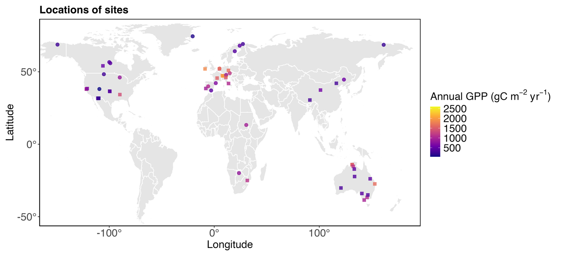
Figure B1Locations of all 56 PLUMBER2 sites used in this study as well as the non-PLUMBER2 sites ES-LMa and US-Tol with mean annual GPP from EC data. The 37 sites used in the EOS analysis (Fig. 5c and d) are highlighted using square shapes.
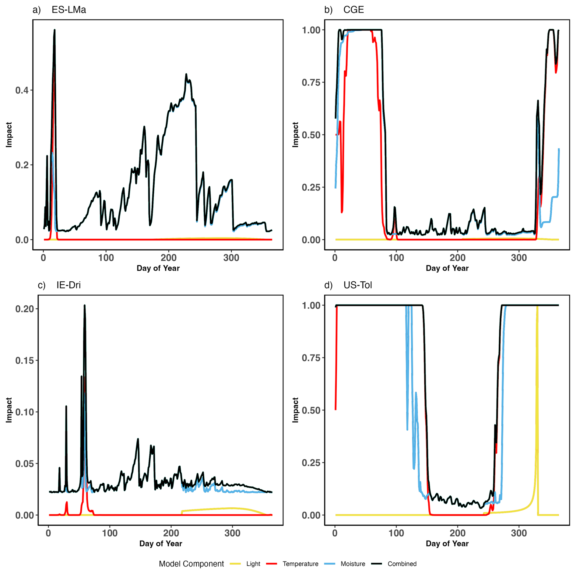
Figure B2The three components of the dynamic leaf turnover model, temperature (red), moisture (blue) and day length (orange) response and their combined impact (green) at the four main sites ES-LMa (a), CGE (b), IE-Dri (c) and US-Tol (d). ES-LMa shows mostly moisture-driven leaf turnover, CGE temperature-driven leaf turnover, IE-Dri is slightly controlled by moisture and US-Tol shows a combination of all three.
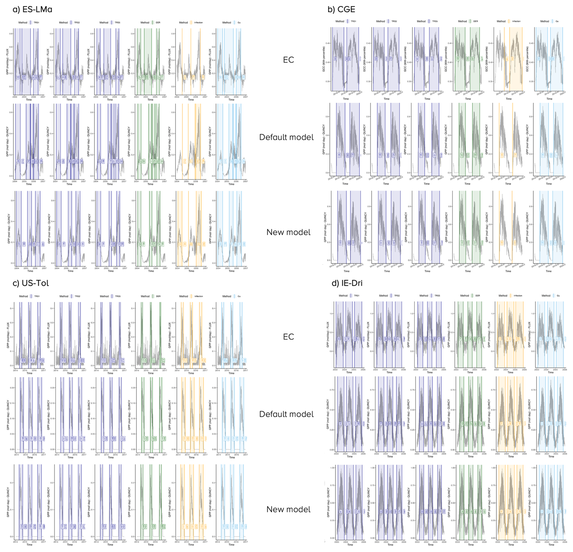
Figure B3GPP from EC data, default and dynamic model at the four main sites with comparison of different methods of the “phenofit” package (Kong et al., 2022): threshold 10 % (TRS1), 20 % (TRS2), 50 % (TRS5), derivative (the method used in our study), Inflection and Gu. The vertical solid lines show the start and end of the season (day of the year) with the growing seasons between them as indicated by the shaded areas.
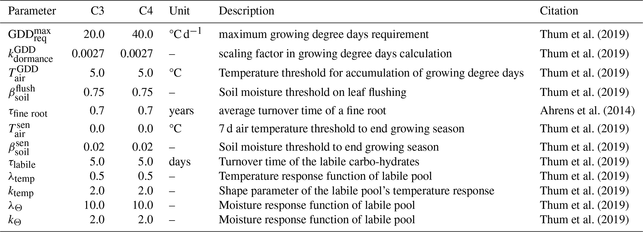
Table C2Mean annual GPP (g C m−2 yr−1), Mean absolute Error (MAE), Root Mean Square Error (RMSE), Normalized Root Mean Square Error (NRMSE) of mean annual GPP across 13 Köppen–Geiger climate classes (“KG class”, 56 flux sites) for the default and dynamic model.
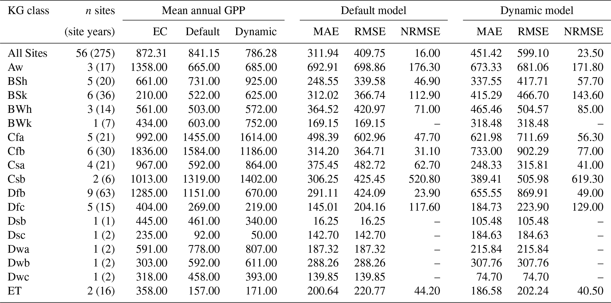
Table C3Dynamic and default model mean annual ecosystem C, vegetation C and SOC (kg m−2) across four sites and 23 years (2000–2022) with t-statistics, df and p value from Welch's t test (Fig. 4).
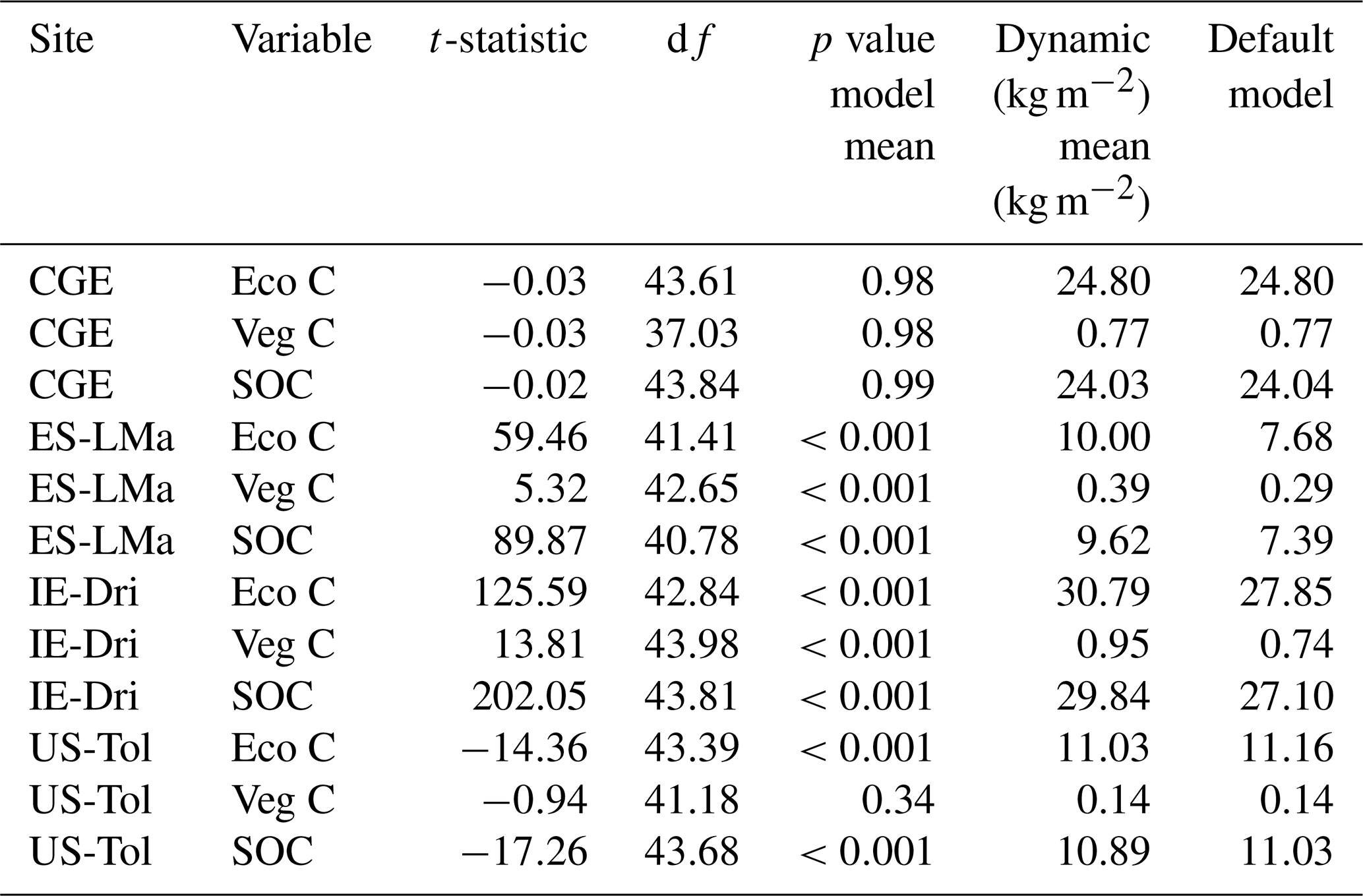
Table C4Depth intervals and layer thickness of the 15 soil layers in QUINCY.
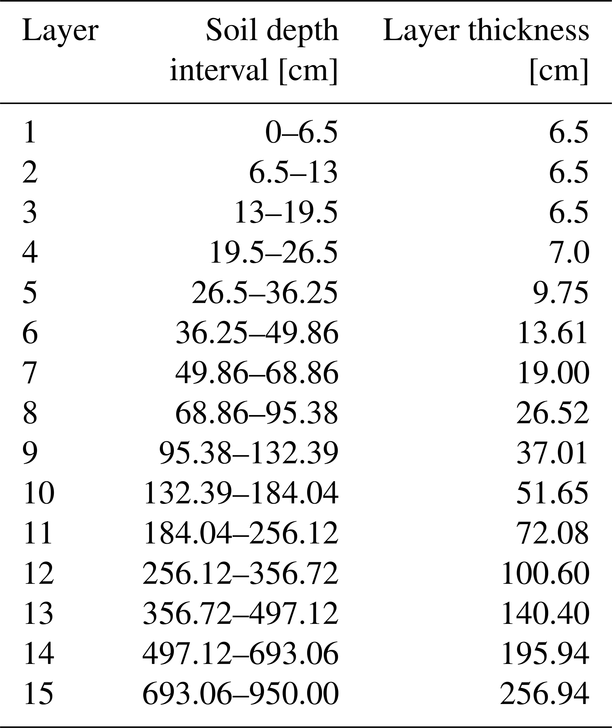
The QUINCY model codes are available under a GPL v3 license. The scientific code of QUINCY relies on software infrastructure from the MPI-ESM environment, which is subject to the MPI-M License Agreement in its most recent form (https://www.bgc-jena.mpg.de/bsi/bsi-data/software/quincy-software/quincy-software-releases, last access: 31 August 2026). The QUINCY source code is available online via MPI-BGC (2019) at https://doi.org/10.17871/quincy-model-2019, but access is limited to registered users. Readers interested in running the model should request a username and password via the Git repository. Model users are strongly encouraged to follow the fair-use policy (https://www.bgc-jena.mpg.de/bsi/bsi-data/software/quincy-software/quincy-software-releases, last access: 31 August 2026). Further, QUINCY as part of the ICON-Land model is published at https://doi.org/10.5281/zenodo.17085112 (de Vrese, 2025) and the latest ICON-ESM release is hosted publicly available at https://gitlab.dkrz.de/icon/icon-model (last access: 13 February 2026) (Müller et al., 2025) under a permissive open source license (BSD-3C). The latest The R code used for statistical analyses and figures as well as the modified QUINCY turnover code are openly available in Zenodo at https://doi.org/10.5281/zenodo.18659433 (Seitz et al., 2026). PLUMBER2 data used for forcing and evaluation is available at https://doi.org/10.25914/5fdb0902607e1 (Ukkola, 2020). ES-LMa GPP data for 2015 to 2018 is available at https://doi.org/10.5281/zenodo.1314194 (Carrara et al., 2018) and PhenoCam data for ES-LMa, CGE and US-Tol is available at https://doi.org/10.3334/ORNLDAAC/2389 (Zimmerman et al., 2025) (PhenoCam site names: eslma, gumpenstein and NEON.D18.TOOL.DP1.00033).
The supplement related to this article is available online at https://doi.org/10.5194/gmd-19-8289-2026-supplement.
JS and SC developed the model. JY contributed to the development of the initial model concept. YZ, FL and SZ developed the general model and gave feedback on the development of the grass phenology model. MY performed the EOS date analysis. LJ, YPL, AS and MB processed and provided the eddy covariance and PhenoCam data for ES-LMa and CGE. All authors contributed to the revision of the manuscript.
The contact author has declared that none of the authors has any competing interests.
Publisher's note: Copernicus Publications remains neutral with regard to jurisdictional claims made in the text, published maps, institutional affiliations, or any other geographical representation in this paper. The authors bear the ultimate responsibility for providing appropriate place names. Views expressed in the text are those of the authors and do not necessarily reflect the views of the publisher.
Data used in this research were provided by the PhenoCam Network, which has been supported by the National Science Foundation, the Long-Term Agroecosystem Research (LTAR) network which is supported by the United States Department of Agriculture (USDA), the US Department of Energy, the US Geological Survey, the Northeastern States Research Cooperative, and the USA National Phenology Network. We thank the PhenoCam Network collaborators, including site PIs and technicians, for publicly sharing the data that were used in this paper.
This research has been supported by the Science Foundation Ireland (grant no. 13/RC/2092_P2), the Trinity Research Doctorate Awards, the Swiss National Science Foundation (Project no. 10003326), the Swiss National Research Foundation (grant PZ00P2_216442), the Deutsche Forschungsgemeinschaft (grant no. 514539694), the Austrian Academy of Sciences (project “ClimGrassHydro”), the Austrian Science Fund (grant no. P28572) and the DaFNE project “ClimGrassEco” (grant no. 101067).
This paper was edited by Hisashi Sato and reviewed by two anonymous referees.
Abramowitz, G., Ukkola, A., Hobeichi, S., Cranko Page, J., Lipson, M., De Kauwe, M. G., Green, S., Brenner, C., Frame, J., Nearing, G., Clark, M., Best, M., Anthoni, P., Arduini, G., Boussetta, S., Caldararu, S., Cho, K., Cuntz, M., Fairbairn, D., Ferguson, C. R., Kim, H., Kim, Y., Knauer, J., Lawrence, D., Luo, X., Malyshev, S., Nitta, T., Ogee, J., Oleson, K., Ottlé, C., Peylin, P., De Rosnay, P., Rumbold, H., Su, B., Vuichard, N., Walker, A. P., Wang-Faivre, X., Wang, Y., and Zeng, Y.: On the predictability of turbulent fluxes from land: PLUMBER2 MIP experimental description and preliminary results, Biogeosciences, 21, 5517–5538, https://doi.org/10.5194/bg-21-5517-2024, 2024. a
Ahrens, B., Hansson, K., Solly, E. F., and Schrumpf, M.: Reconcilable differences: a joint calibration of fine‐root turnover times with radiocarbon and minirhizotrons, New Phytol., 204, 932–942, https://doi.org/10.1111/nph.12979, 2014. a, b
Arndt, K. A., Santos, M. J., Ustin, S., Davidson, S. J., Stow, D., Oechel, W. C., Tran, T. T. P., Graybill, B., and Zona, D.: Arctic greening associated with lengthening growing seasons in Northern Alaska, Environ. Res. Lett., 14, 125018, https://doi.org/10.1088/1748-9326/ab5e26, 2019. a
Bai, Y. and Cotrufo, M. F.: Grassland soil carbon sequestration: Current understanding, challenges, and solutions, Science, 377, 603–608, https://doi.org/10.1126/science.abo2380, 2022. a, b
Balzarolo, M., Boussetta, S., Balsamo, G., Beljaars, A., Maignan, F., Calvet, J.-C., Lafont, S., Barbu, A., Poulter, B., Chevallier, F., Szczypta, C., and Papale, D.: Evaluating the potential of large-scale simulations to predict carbon fluxes of terrestrial ecosystems over a European Eddy Covariance network, Biogeosciences, 11, 2661–2678, https://doi.org/10.5194/bg-11-2661-2014, 2014. a, b, c
Beck, H. E., Zimmermann, N. E., McVicar, T. R., Vergopolan, N., Berg, A., and Wood, E. F.: Present and future Köppen–Geiger climate classification maps at 1-km resolution, Sci. Data, 5, 180214, https://doi.org/10.1038/sdata.2018.214, 2018. a
Bengtsson, J., Bullock, J. M., Egoh, B., Everson, C., Everson, T., O'Connor, T., O'Farrell, P. J., Smith, H. G., and Lindborg, R.: Grasslands – more important for ecosystem services than you might think, Ecosphere, 10, e02582, https://doi.org/10.1002/ecs2.2582, 2019. a
Bórnez, K., Richardson, A. D., Verger, A., Descals, A., and Peñuelas, J.: Evaluation of VEGETATION and PROBA-V Phenology Using PhenoCam and Eddy Covariance Data, Remote Sens., 12, 3077, https://doi.org/10.3390/rs12183077, 2020. a
Brahney, J., Mahowald, N., Ward, D. S., Ballantyne, A. P., and Neff, J. C.: Is atmospheric phosphorus pollution altering global alpine Lake stoichiometry?, Global Biogeochem. Cy., 29, 1369–1383, https://doi.org/10.1002/2015GB005137, 2015. a
Butler, E. E., Wythers, K. R., Flores‐Moreno, H., Ricciuto, D. M., Datta, A., Banerjee, A., Atkin, O. K., Kattge, J., Thornton, P. E., Anand, M., Burrascano, S., Byun, C., Cornelissen, J. H. C., Forey, E., Jansen, S., Kramer, K., Minden, V., and Reich, P. B.: Increasing Functional Diversity in a Global Land Surface Model Illustrates Uncertainties Related to Parameter Simplification, J. Geophys. Res.-Biogeo., 127, e2021JG006606, https://doi.org/10.1029/2021JG006606, 2022. a
Caldararu, S., Thum, T., Yu, L., and Zaehle, S.: Whole-plant optimality predicts changes in leaf nitrogen under variable CO2 and nutrient availability, New Phytol., 225, 2331–2346, https://doi.org/10.1111/nph.16327, 2020. a
Caldararu, S., Thum, T., Yu, L., Kern, M., Nair, R., and Zaehle, S.: Long-term ecosystem nitrogen limitation from foliar δ15N data and a land surface model, Global Change Biol., 28, 493–508, https://doi.org/10.1111/gcb.15933, 2021. a
Carrara, A., El-Madany, T. S., Lopez-Jimenez, R., Hertel, M., Kolle, O., Knauer, J., Perez-Priego, O., Reichstein, M., Zaehle, S., and Migliavacca, M.: Majadas de Tietar: Ecosystem level and understorey carbon, water, and energy fluxes in a Mediterranean tree-grass ecosystem (1.0), Zenodo [data set], https://doi.org/10.5281/zenodo.1314194, 2018. a
Chapin III, F. S., Jefferies, R. L., Reynolds, J. F., Shaver, G. R., Svoboda, J., and Chu, E. W.: Arctic ecosystems in a changing climate: an ecophysiological perspective, Academic Press, ISBN 0-323-13842-X, 2012. a, b, c
Chen, S., Fu, Y. H., Li, M., Jia, Z., Cui, Y., and Tang, J.: A new temperature–photoperiod coupled phenology module in LPJ-GUESS model v4.1: optimizing estimation of terrestrial carbon and water processes, Geosci. Model Dev., 17, 2509–2523, https://doi.org/10.5194/gmd-17-2509-2024, 2024. a, b, c
Chen, X., An, S., Inouye, D. W., and Schwartz, M. D.: Temperature and snowfall trigger alpine vegetation green‐up on the world's roof, Global Change Biol., 21, 3635–3646, https://doi.org/10.1111/gcb.12954, 2015. a
Cherwin, K. and Knapp, A.: Unexpected patterns of sensitivity to drought in three semi-arid grasslands, Oecologia, 169, 845–852, https://doi.org/10.1007/s00442-011-2235-2, 2012. a, b
Chien, C., Mackey, K. R. M., Dutkiewicz, S., Mahowald, N. M., Prospero, J. M., and Paytan, A.: Effects of African dust deposition on phytoplankton in the western tropical Atlantic Ocean off Barbados, Global Biogeochem. Cy., 30, 716–734, https://doi.org/10.1002/2015GB005334, 2016. a
Cooper, P.: The absorption of radiation in solar stills, Solar Energy, 12, 333–346, 1969. a
De Kauwe, M. G., Zhou, S.-X., Medlyn, B. E., Pitman, A. J., Wang, Y.-P., Duursma, R. A., and Prentice, I. C.: Do land surface models need to include differential plant species responses to drought? Examining model predictions across a mesic-xeric gradient in Europe, Biogeosciences, 12, 7503–7518, https://doi.org/10.5194/bg-12-7503-2015, 2015. a
De Kauwe, M. G., Medlyn, B. E., Walker, A. P., Zaehle, S., Asao, S., Guenet, B., Harper, A. B., Hickler, T., Jain, A. K., Luo, Y., Lu, X., Luus, K., Parton, W. J., Shu, S., Wang, Y. P., Werner, C., Xia, J., Pendall, E., Morgan, J. A., Ryan, E. M., Carrillo, Y., Dijkstra, F. A., Zelikova, T. J., and Norby, R. J.: Challenging terrestrial biosphere models with data from the long-term multifactor Prairie Heating and CO2 Enrichment experiment, Global Change Biol., 23, 3623–3645, https://doi.org/10.1111/gcb.13643, 2017. a, b
de Vrese, P.: ICON-Land: Tile-based representation of lateral exchange processes, Zenodo [code], https://doi.org/10.5281/zenodo.17085112, 2025. a
Dixon, A. P., Faber‐Langendoen, D., Josse, C., Morrison, J., and Loucks, C. J.: Distribution mapping of world grassland types, J. Biogeogr., 41, 2003–2019, https://doi.org/10.1111/jbi.12381, 2014. a
Dragoni, D., Schmid, H. P., Wayson, C. A., Potter, H., Grimmond, C. S. B., and Randolph, J. C.: Evidence of increased net ecosystem productivity associated with a longer vegetated season in a deciduous forest in south‐central Indiana, USA, Global Change Biol., 17, 886–897, https://doi.org/10.1111/j.1365-2486.2010.02281.x, 2011. a
Elmore, A. J., Guinn, S. M., Minsley, B. J., and Richardson, A. D.: Landscape controls on the timing of spring, autumn, and growing season length in mid-Atlantic forests, Global Change Biol., 18, 656–674, https://doi.org/10.1111/j.1365-2486.2011.02521.x, 2012. a
Estiarte, M. and Peñuelas, J.: Alteration of the phenology of leaf senescence and fall in winter deciduous species by climate change: effects on nutrient proficiency, Global Change Biol., 21, 1005–1017, https://doi.org/10.1111/gcb.12804, 2015. a
Fang, Q., Wang, G., Xue, B., Liu, T., and Kiem, A.: How and to what extent does precipitation on multi-temporal scales and soil moisture at different depths determine carbon flux responses in a water-limited grassland ecosystem?, Sci. Total Environ., 635, 1255–1266, https://doi.org/10.1016/j.scitotenv.2018.04.225, 2018. a
Felton, A. J. and Goldsmith, G. R.: Timing and magnitude of drought impacts on carbon uptake across a grassland biome, Global Change Biol., 29, 2790–2803, https://doi.org/10.1111/gcb.16637, 2023. a
Fisher, J. B., Huntzinger, D. N., Schwalm, C. R., and Sitch, S.: Modeling the Terrestrial Biosphere, Annu. Rev. Environ. Resour., 39, 91–123, https://doi.org/10.1146/annurev-environ-012913-093456, 2014. a
Fu, Y. H., Campioli, M., Demarée, G., Deckmyn, A., Hamdi, R., Janssens, I. A., and Deckmyn, G.: Bayesian calibration of the Unified budburst model in six temperate tree species, Int. J. Biometeorol., 56, 153–164, 2012. a
Halpern, B. S., Walbridge, S., Selkoe, K. A., Kappel, C. V., Micheli, F., D'Agrosa, C., Bruno, J. F., Casey, K. S., Ebert, C., Fox, H. E., Fujita, R., Heinemann, D., Lenihan, H. S., Madin, E. M. P., Perry, M. T., Selig, E. R., Spalding, M., Steneck, R., and Watson, R.: A Global Map of Human Impact on Marine Ecosystems, Science, 319, 948–952, https://doi.org/10.1126/science.1149345, 2008. a
Harrison, S. P., Prentice, I. C., Barboni, D., Kohfeld, K. E., Ni, J., and Sutra, J.-P.: Ecophysiological and bioclimatic foundations for a global plant functional classification, J. Veg. Sci., 21, 300–317, https://doi.org/10.1111/j.1654-1103.2009.01144.x, 2010. a
Haynes, K. D., Baker, I. T., Denning, A. S., Wolf, S., Wohlfahrt, G., Kiely, G., Minaya, R. C., and Haynes, J. M.: Representing Grasslands Using Dynamic Prognostic Phenology Based on Biological Growth Stages: Part 2. Carbon Cycling, J. Adv. Model. Earth Syst., 11, 4440–4465, https://doi.org/10.1029/2018MS001541, 2019. a, b
Hengl, T., Mendes de Jesus, J., Heuvelink, G. B. M., Ruiperez Gonzalez, M., Kilibarda, M., Blagotić, A., Shangguan, W., Wright, M. N., Geng, X., Bauer-Marschallinger, B., Guevara, M. A., Vargas, R., MacMillan, R. A., Batjes, N. H., Leenaars, J. G. B., Ribeiro, E., Wheeler, I., Mantel, S., and Kempen, B.: SoilGrids250m: Global gridded soil information based on machine learning, PLOS ONE, 12, e0169748, https://doi.org/10.1371/journal.pone.0169748, 2017. a
Hickler, T., Prentice, I. C., Smith, B., Sykes, M. T., and Zaehle, S.: Implementing plant hydraulic architecture within the LPJ Dynamic Global Vegetation Model, Global Ecol. Biogeogr., 15, 567–577, 2006. a
Hollinger, D. Y., Aber, J., Dail, B., Davidson, E. A., Goltz, S. M., Hughes, H., Leclerc, M. Y., Lee, J. T., Richardson, A. D., Rodrigues, C., Scott, N., Achuatavarier, D., and Walsh, J.: Spatial and temporal variability in forest–atmosphere CO2 exchange, Global Change Biol., 10, 1689–1706, https://doi.org/10.1111/j.1365-2486.2004.00847.x, 2004. a
Jeong, S.-J., Ho, C.-H., Gim, H.-J., and Brown, M. E.: Phenology shifts at start vs. end of growing season in temperate vegetation over the Northern Hemisphere for the period 1982–2008: phenology shifts at start vs. end of growing season, Global Change Biol., 17, 2385–2399, https://doi.org/10.1111/j.1365-2486.2011.02397.x, 2011. a
Jönsson, P. and Eklundh, L.: TIMESAT – a program for analyzing time-series of satellite sensor data, Comput. Geosci., 30, 833–845, https://doi.org/10.1016/j.cageo.2004.05.006, 2004. a
Joseph, L. S. K., Cremonese, E., Migliavacca, M., Schaumberger, A., and Bahn, M.: Warming, elevated CO2 and drought in combination amplify shifts in canopy greenness dynamics in managed grassland, Agr. Ecosyst. Environ., 378, 109304, https://doi.org/10.1016/j.agee.2024.109304, 2025. a
Kattge, J., Díaz, S., Lavorel, S., Prentice, I. C., Leadley, P., Bönisch, G., Garnier, E., Westoby, M., Reich, P. B., Wright, I. J., Cornelissen, J. H. C., Violle, C., Harrison, S. P., Van Bodegom, P. M., Reichstein, M., Enquist, B. J., Soudzilovskaia, N. A., Ackerly, D. D., Anand, M., Atkin, O., Bahn, M., Baker, T. R., Baldocchi, D., Bekker, R., Blanco, C. C., Blonder, B., Bond, W. J., Bradstock, R., Bunker, D. E., Casanoves, F., Cavender-Bares, J., Chambers, J. Q., Chapin Iii, F. S., Chave, J., Coomes, D., Cornwell, W. K., Craine, J. M., Dobrin, B. H., Duarte, L., Durka, W., Elser, J., Esser, G., Estiarte, M., Fagan, W. F., Fang, J., Fernández‐Méndez, F., Fidelis, A., Finegan, B., Flores, O., Ford, H., Frank, D., Freschet, G. T., Fyllas, N. M., Gallagher, R. V., Green, W. A., Gutierrez, A. G., Hickler, T., Higgins, S. I., Hodgson, J. G., Jalili, A., Jansen, S., Joly, C. A., Kerkhoff, A. J., Kirkup, D., Kitajima, K., Kleyer, M., Klotz, S., Knops, J. M. H., Kramer, K., Kühn, I., Kurokawa, H., Laughlin, D., Lee, T. D., Leishman, M., Lens, F., Lenz, T., Lewis, S. L., Lloyd, J., Llusià, J., Louault, F., Ma, S., Mahecha, M. D., Manning, P., Massad, T., Medlyn, B. E., Messier, J., Moles, A. T., Müller, S. C., Nadrowski, K., Naeem, S., Niinemets, U., Nöllert, S., Nüske, A., Ogaya, R., Oleksyn, J., Onipchenko, V. G., Onoda, Y., Ordoñez, J., Overbeck, G., Ozinga, W. A., Patiño, S., Paula, S., Pausas, J. G., Peñuelas, J., Phillips, O. L., Pillar, V., Poorter, H., Poorter, L., Poschlod, P., Prinzing, A., Proulx, R., Rammig, A., Reinsch, S., Reu, B., Sack, L., Salgado‐Negret, B., Sardans, J., Shiodera, S., Shipley, B., Siefert, A., Sosinski, E., Soussana, J., Swaine, E., Swenson, N., Thompson, K., Thornton, P., Waldram, M., Weiher, E., White, M., White, S., Wright, S. J., Yguel, B., Zaehle, S., Zanne, A. E., and Wirth, C.: TRY – a global database of plant traits, Global Change Biol., 17, 2905–2935, https://doi.org/10.1111/j.1365-2486.2011.02451.x, 2011. a, b
Keenan, T. F., Darby, B., Felts, E., Sonnentag, O., Friedl, M. A., Hufkens, K., O'Keefe, J., Klosterman, S., Munger, J. W., Toomey, M., and Richardson, A. D.: Tracking forest phenology and seasonal physiology using digital repeat photography: a critical assessment, Ecol. Appl., 24, 1478–1489, https://doi.org/10.1890/13-0652.1, 2014. a, b
Kennedy, C. M., Oakleaf, J. R., Theobald, D. M., Baruch‐Mordo, S., and Kiesecker, J.: Managing the middle: A shift in conservation priorities based on the global human modification gradient, Global Change Biol., 25, 811–826, https://doi.org/10.1111/gcb.14549, 2019. a
Kiely, G., Leahy, P., Lewis, C., Sottocornola, M., Laine, A., and Koehler, A.-K.: GHG fluxes from terrestrial ecosystems in Ireland: CCRP08Proj-1.1A, Tech. rep., Environmental Protection Agency, Johnstown Castle, Co. Wexford, Ireland, https://www.epa.ie/publications/research/reports/research-227-ghg-fluxes-from-terrestrial-ecosystems-in-ireland.php (last access: 29 March 2025), 2018. a
Kong, D., Zhang, Y., Wang, D., Chen, J., and Gu, X.: Photoperiod Explains the Asynchronization Between Vegetation Carbon Phenology and Vegetation Greenness Phenology, J. Geophys. Res.-Biogeo., 125, e2020JG005636, https://doi.org/10.1029/2020JG005636, 2020. a
Kong, D., McVicar, T. R., Xiao, M., Zhang, Y., Peña‐Arancibia, J. L., Filippa, G., Xie, Y., and Gu, X.: phenofit : An R package for extracting vegetation phenology from time series remote sensing, Meth. Ecol. Evol., 13, 1508–1527, https://doi.org/10.1111/2041-210X.13870, 2022. a, b, c, d, e
Körner, C.: Plant adaptation to cold climates, F1000Research, 5, 2769, https://doi.org/10.12688/f1000research.9107.1, 2016. a, b
Kou-Giesbrecht, S., Arora, V. K., Seiler, C., Arneth, A., Falk, S., Jain, A. K., Joos, F., Kennedy, D., Knauer, J., Sitch, S., O'Sullivan, M., Pan, N., Sun, Q., Tian, H., Vuichard, N., and Zaehle, S.: Evaluating nitrogen cycling in terrestrial biosphere models: a disconnect between the carbon and nitrogen cycles, Earth Syst. Dynam., 14, 767–795, https://doi.org/10.5194/esd-14-767-2023, 2023. a
Krinner, G., Viovy, N., De Noblet‐Ducoudré, N., Ogée, J., Polcher, J., Friedlingstein, P., Ciais, P., Sitch, S., and Prentice, I. C.: A dynamic global vegetation model for studies of the coupled atmosphere‐biosphere system, Global Biogeochem. Cy., 19, 2003GB002199, https://doi.org/10.1029/2003GB002199, 2005. a
Lacroix, F., Zaehle, S., Caldararu, S., Schaller, J., Stimmler, P., Holl, D., Kutzbach, L., and Göckede, M.: Mismatch of N release from the permafrost and vegetative uptake opens pathways of increasing nitrous oxide emissions in the high Arctic, Global Change Biol., 28, 5973–5990, https://doi.org/10.1111/gcb.16345, 2022. a, b, c, d
Lamarque, J.-F., Bond, T. C., Eyring, V., Granier, C., Heil, A., Klimont, Z., Lee, D., Liousse, C., Mieville, A., Owen, B., Schultz, M. G., Shindell, D., Smith, S. J., Stehfest, E., Van Aardenne, J., Cooper, O. R., Kainuma, M., Mahowald, N., McConnell, J. R., Naik, V., Riahi, K., and Van Vuuren, D. P.: Historical (1850–2000) gridded anthropogenic and biomass burning emissions of reactive gases and aerosols: methodology and application, Atmos. Chem. Phys., 10, 7017–7039, https://doi.org/10.5194/acp-10-7017-2010, 2010. a
Lamarque, J.-F., Kyle, G. P., Meinshausen, M., Riahi, K., Smith, S. J., Van Vuuren, D. P., Conley, A. J., and Vitt, F.: Global and regional evolution of short-lived radiatively-active gases and aerosols in the Representative Concentration Pathways, Climatic Change, 109, 191–212, https://doi.org/10.1007/s10584-011-0155-0, 2011. a
Lang, W., Chen, X., Qian, S., Liu, G., and Piao, S.: A new process-based model for predicting autumn phenology: How is leaf senescence controlled by photoperiod and temperature coupling?, Agr. Forest Meteorol., 268, 124–135, https://doi.org/10.1016/j.agrformet.2019.01.006, 2019. a, b, c, d, e, f, g
Lawrence, D. M., Fisher, R. A., Koven, C. D., Oleson, K. W., Swenson, S. C., Bonan, G., Collier, N., Ghimire, B., Van Kampenhout, L., Kennedy, D., Kluzek, E., Lawrence, P. J., Li, F., Li, H., Lombardozzi, D., Riley, W. J., Sacks, W. J., Shi, M., Vertenstein, M., Wieder, W. R., Xu, C., Ali, A. A., Badger, A. M., Bisht, G., Van Den Broeke, M., Brunke, M. A., Burns, S. P., Buzan, J., Clark, M., Craig, A., Dahlin, K., Drewniak, B., Fisher, J. B., Flanner, M., Fox, A. M., Gentine, P., Hoffman, F., Keppel‐Aleks, G., Knox, R., Kumar, S., Lenaerts, J., Leung, L. R., Lipscomb, W. H., Lu, Y., Pandey, A., Pelletier, J. D., Perket, J., Randerson, J. T., Ricciuto, D. M., Sanderson, B. M., Slater, A., Subin, Z. M., Tang, J., Thomas, R. Q., Val Martin, M., and Zeng, X.: The Community Land Model Version 5: Description of New Features, Benchmarking, and Impact of Forcing Uncertainty, J. Adv. Model. Earth Syst., 11, 4245–4287, https://doi.org/10.1029/2018MS001583, 2019. a
Lemaire, G., Hodgson, J., and Chabbi, A.: Introduction: Food security and environmental impacts – challenge for grassland sciences, in: Grassland Productivity and Ecosystem Services, edited by: Lemaire, G., Hodgson, J., and Chabbi, A., CAB International, Wallingford, UK, xiii–xvii, https://doi.org/10.1079/9781845938093.0000, 2011. a
Le Quéré, C., Andrew, R. M., Friedlingstein, P., Sitch, S., Hauck, J., Pongratz, J., Pickers, P. A., Korsbakken, J. I., Peters, G. P., Canadell, J. G., Arneth, A., Arora, V. K., Barbero, L., Bastos, A., Bopp, L., Chevallier, F., Chini, L. P., Ciais, P., Doney, S. C., Gkritzalis, T., Goll, D. S., Harris, I., Haverd, V., Hoffman, F. M., Hoppema, M., Houghton, R. A., Hurtt, G., Ilyina, T., Jain, A. K., Johannessen, T., Jones, C. D., Kato, E., Keeling, R. F., Goldewijk, K. K., Landschützer, P., Lefèvre, N., Lienert, S., Liu, Z., Lombardozzi, D., Metzl, N., Munro, D. R., Nabel, J. E. M. S., Nakaoka, S.-I., Neill, C., Olsen, A., Ono, T., Patra, P., Peregon, A., Peters, W., Peylin, P., Pfeil, B., Pierrot, D., Poulter, B., Rehder, G., Resplandy, L., Robertson, E., Rocher, M., Rödenbeck, C., Schuster, U., Schwinger, J., Séférian, R., Skjelvan, I., Steinhoff, T., Sutton, A., Tans, P. P., Tian, H., Tilbrook, B., Tubiello, F. N., Van Der Laan-Luijkx, I. T., Van Der Werf, G. R., Viovy, N., Walker, A. P., Wiltshire, A. J., Wright, R., Zaehle, S., and Zheng, B.: Global Carbon Budget 2018, Earth Syst. Sci. Data, 10, 2141–2194, https://doi.org/10.5194/essd-10-2141-2018, 2018. a
Levitt, J.: Responses of Plants to Environmental Stresses, Vol. 1: Chilling, Freezing, and High Temperature Stresses, 2nd edn., Academic Press, New York, NY, USA, https://doi.org/10.1016/B978-0-12-445501-6.50016-6, 1980. a
Luo, Y., El-Madany, T. S., Filippa, G., Ma, X., Ahrens, B., Carrara, A., Gonzalez-Cascon, R., Cremonese, E., Galvagno, M., Hammer, T. W., Pacheco-Labrador, J., Martín, M. P., Moreno, G., Perez-Priego, O., Reichstein, M., Richardson, A. D., Römermann, C., and Migliavacca, M.: Using Near-Infrared-Enabled Digital Repeat Photography to Track Structural and Physiological Phenology in Mediterranean Tree–Grass Ecosystems, Remote Sens., 10, https://doi.org/10.3390/rs10081293, 2018. a
Luo, Y., Gessler, A., D'Odorico, P., Hufkens, K., and Stocker, B. D.: Quantifying effects of cold acclimation and delayed springtime photosynthesis resumption in northern ecosystems, New Phytol., 240, 984–1002, https://doi.org/10.1111/nph.19208, 2023. a
Mäkelä, A., Hari, P., Berninger, F., Hanninen, H., and Nikinmaa, E.: Acclimation of photosynthetic capacity in Scots pine to the annual cycle of temperature, Tree Physiol., 24, 369–376, https://doi.org/10.1093/treephys/24.4.369, 2004. a
Mäkelä, A., Pulkkinen, M., Kolari, P., Lagergren, F., Berbigier, P., Lindroth, A., Loustau, D., Nikinmaa, E., Vesala, T., and Hari, P.: Developing an empirical model of stand GPP with the LUE approach: analysis of eddy covariance data at five contrasting conifer sites in Europe, Global Change Biol., 14, 92–108, https://doi.org/10.1111/j.1365-2486.2007.01463.x, 2008. a
Medlyn, B. E., Duursma, R. A., Eamus, D., Ellsworth, D. S., Prentice, I. C., Barton, C. V. M., Crous, K. Y., De Angelis, P., Freeman, M., and Wingate, L.: Reconciling the optimal and empirical approaches to modelling stomatal conductance: reconciling optimal and empirical stomatal models, Global Change Biol., 17, 2134–2144, https://doi.org/10.1111/j.1365-2486.2010.02375.x, 2011. a
Miinalainen, T., Ojasalo, A., Croft, H., Aurela, M., Peltoniemi, M., Caldararu, S., Zaehle, S., and Thum, T.: Evaluating the carbon and nitrogen cycles of the QUINCY terrestrial biosphere model using space-born optical remotely-sensed data, Biogeosciences, 22, 6937–6962, https://doi.org/10.5194/bg-22-6937-2025, 2025. a
MPI-BGC: QUINCY model, MPI-BGC [code], https://doi.org/10.17871/quincy-model-2019, 2019. a
Müller, W. A., Lorenz, S., Pham, T. V., Schneidereit, A., Brokopf, R., Brovkin, V., Brüggemann, N., Chegini, F., Dommenget, D., Fröhlich, K., Früh, B., Gayler, V., Haak, H., Hagemann, S., Hanke, M., Ilyina, T., Jungclaus, J., Köhler, M., Korn, P., Kornblueh, L., Kroll, C. A., Krüger, J., Castro-Morales, K., Niemeier, U., Pohlmann, H., Polkova, I., Potthast, R., Riddick, T., Schlund, M., Stacke, T., Wirth, R., Yu, D., and Marotzke, J.: The ICON-based Earth System Model for climate predictions and projections (ICON XPP v1.0), Geosci. Model Dev., 18, 9385–9415, https://doi.org/10.5194/gmd-18-9385-2025, 2025. a
Myers‐Smith, I. H., Grabowski, M. M., Thomas, H. J. D., Angers‐Blondin, S., Daskalova, G. N., Bjorkman, A. D., Cunliffe, A. M., Assmann, J. J., Boyle, J. S., McLeod, E., McLeod, S., Joe, R., Lennie, P., Arey, D., Gordon, R. R., and Eckert, C. D.: Eighteen years of ecological monitoring reveals multiple lines of evidence for tundra vegetation change, Ecol. Monogr., 89, e01351, https://doi.org/10.1002/ecm.1351, 2019. a
Nair, R., Luo, Y., El‐Madany, T., Rolo, V., Pacheco‐Labrador, J., Caldararu, S., Morris, K. A., Schrumpf, M., Carrara, A., Moreno, G., Reichstein, M., and Migliavacca, M.: Nitrogen availability and summer drought, but not N:P imbalance, drive carbon use efficiency of a Mediterranean tree‐grass ecosystem, Global Change Biol., 30, e17486, https://doi.org/10.1111/gcb.17486, 2024. a, b
Parton, W. J., ScurlockD, M. O., Ojima, S., Gilmanov, T., Scholes, R., Schimel, D., Kirchner, T., Menaut, J., Seastedt, T., Garcia Moya, E., and Kamnalrut, A.: Observations and modeling of biomass and soil organic matter dynamics for the grassland biome worldwide, Global Biogeochem. Cy., 7, 785–809, 1993. a
Peano, D., Hemming, D., Materia, S., Delire, C., Fan, Y., Joetzjer, E., Lee, H., Nabel, J. E. M. S., Park, T., Peylin, P., Wårlind, D., Wiltshire, A., and Zaehle, S.: Plant phenology evaluation of CRESCENDO land surface models – Part 1: Start and end of the growing season, Biogeosciences, 18, 2405–2428, https://doi.org/10.5194/bg-18-2405-2021, 2021. a
Poppenwimer, T., Mayrose, I., and DeMalach, N.: Revising the global biogeography of annual and perennial plants, Nature, 624, 109–114, https://doi.org/10.1038/s41586-023-06644-x, 2023. a, b
Radolinski, J., Vremec, M., Wachter, H., Birk, S., Brüggemann, N., Herndl, M., Kahmen, A., Nelson, D. B., Kübert, A., Schaumberger, A., Stumpp, C., Tissink, M., Werner, C., and Bahn, M.: Drought in a warmer, CO2-rich climate restricts grassland water use and soil water mixing, Science, 387, 290–296, https://doi.org/10.1126/science.ado0734, 2025. a
R Core Team: R: A Language and Environment for Statistical Computing, R Foundation for Statistical Computing, Vienna, https://www.R-project.org/ (last access: 25 May 2026), 2021. a
Ren, S., Qin, Q., Ren, H., Sui, J., and Zhang, Y.: New model for simulating autumn phenology of herbaceous plants in the Inner Mongolian Grassland, Agr. Forest Meteorol., 275, 136–145, https://doi.org/10.1016/j.agrformet.2019.05.011, 2019. a
Ren, S., Vitasse, Y., Chen, X., Peichl, M., and An, S.: Assessing the relative importance of sunshine, temperature, precipitation, and spring phenology in regulating leaf senescence timing of herbaceous species in China, Agr. Forest Meteorol., 313, 108770, https://doi.org/10.1016/j.agrformet.2021.108770, 2022. a, b, c, d
Richardson, A. D. and O'Keefe, J.: Phenological differences between understory and overstory: a case study using the long-term Harvard Forest records, in: Phenology of Ecosystem Processes: Applications in Global Change Research, edited by: Noormets, A., Springer, New York, NY, USA, 87–117, https://doi.org/10.1007/978-1-4419-0026-5_4, 2009. a
Richardson, A. D., Black, T. A., Ciais, P., Delbart, N., Friedl, M. A., Gobron, N., Hollinger, D. Y., Kutsch, W. L., Longdoz, B., Luyssaert, S., Migliavacca, M., Montagnani, L., Munger, J. W., Moors, E., Piao, S., Rebmann, C., Reichstein, M., Saigusa, N., Tomelleri, E., Vargas, R., and Varlagin, A.: Influence of spring and autumn phenological transitions on forest ecosystem productivity, Philos. T. R. Soc. B, 365, 3227–3246, https://doi.org/10.1098/rstb.2010.0102, 2010. a
Richardson, A. D., Anderson, R. S., Arain, M. A., Barr, A. G., Bohrer, G., Chen, G., Chen, J. M., Ciais, P., Davis, K. J., Desai, A. R., Dietze, M. C., Dragoni, D., Garrity, S. R., Gough, C. M., Grant, R., Hollinger, D. Y., Margolis, H. A., McCaughey, H., Migliavacca, M., Monson, R. K., Munger, J. W., Poulter, B., Raczka, B. M., Ricciuto, D. M., Sahoo, A. K., Schaefer, K., Tian, H., Vargas, R., Verbeeck, H., Xiao, J., and Xue, Y.: Terrestrial biosphere models need better representation of vegetation phenology: results from the North American Carbon Program Site Synthesis, Global Change Biol., 18, 566–584, https://doi.org/10.1111/j.1365-2486.2011.02562.x, 2012. a, b, c
Richardson, A. D., Keenan, T. F., Migliavacca, M., Ryu, Y., Sonnentag, O., and Toomey, M.: Climate change, phenology, and phenological control of vegetation feedbacks to the climate system, Agr. Forest Meteorol., 169, 156–173, https://doi.org/10.1016/j.agrformet.2012.09.012, 2013. a
Richardson, A. D., Hufkens, K., Milliman, T., Aubrecht, D. M., Chen, M., Gray, J. M., Johnston, M. R., Keenan, T. F., Klosterman, S. T., Kosmala, M., Melaas, E. K., Friedl, M. A., and Frolking, S.: Tracking vegetation phenology across diverse North American biomes using PhenoCam imagery, Sci. Data, 5, 180028, https://doi.org/10.1038/sdata.2018.28, 2018. a, b
Sakuraba, Y.: Light-Mediated Regulation of Leaf Senescence, Int. J. Mol. Sci., 22, https://doi.org/10.3390/ijms22073291, 2021. a, b, c, d
Saxton, K. E. and Rawls, W. J.: Soil Water Characteristic Estimates by Texture and Organic Matter for Hydrologic Solutions, Soil Sci. Soc. Am. J., 70, 1569–1578, https://doi.org/10.2136/sssaj2005.0117, 2006. a, b
Schwalm, C. R., Williams, C. A., Schaefer, K., Anderson, R., Arain, M. A., Baker, I., Barr, A., Black, T. A., Chen, G., Chen, J. M., Ciais, P., Davis, K. J., Desai, A., Dietze, M., Dragoni, D., Fischer, M. L., Flanagan, L. B., Grant, R., Gu, L., Hollinger, D., Izaurralde, R. C., Kucharik, C., Lafleur, P., Law, B. E., Li, L., Li, Z., Liu, S., Lokupitiya, E., Luo, Y., Ma, S., Margolis, H., Matamala, R., McCaughey, H., Monson, R. K., Oechel, W. C., Peng, C., Poulter, B., Price, D. T., Riciutto, D. M., Riley, W., Sahoo, A. K., Sprintsin, M., Sun, J., Tian, H., Tonitto, C., Verbeeck, H., and Verma, S. B.: A model‐data intercomparison of CO2 exchange across North America: Results from the North American Carbon Program site synthesis, J. Geophys. Res.-Biogeo., 115, 2009JG001229, https://doi.org/10.1029/2009JG001229, 2010. a
Scurlock, J. M. O. and Hall, D. O.: The global carbon sink: a grassland perspective, Global Change Biol., 4, 229–233, https://doi.org/10.1046/j.1365-2486.1998.00151.x, 1998. a
Seitz, J. I., Yajima, M., Joseph, L. S. K., Yang, J., Lacroix, F., Luo, Y., Schaumberger, A., Bahn, M., Zaehle, S., and Caldararu, S.: Scripts for “A general physiologically driven representation of leaf turnover in grasslands in the QUINCY land surface model (revision: 974a6b7f)”, Zenodo [code], https://doi.org/10.5281/zenodo.18659433, 2026. a
Seyednasrollah, B.: Phenocamapi R Package: Interacting with the PhenoCam server, Zenodo [code], https://doi.org/10.5281/zenodo.1464365, 2018. a
Seyednasrollah, B., Young, A., Hufkens, K., Milliman, T., Friedl, M., Frolking, S., Richardson, A., Abraha, M., Allen, D., Apple, M., Arain, M., Baker, J., Baker, J., Baldocchi, D., Bernacchi, C., Bhattacharjee, J., Blanken, P., Bosch, D., Boughton, R., Boughton, E., Brown, R., Browning, D., Brunsell, N., Burns, S., Cavagna, M., Chu, H., Clark, P., Conrad, B., Cremonese, E., Debinski, D., Desai, A., Diaz-Delgado, R., Duchesne, L., Dunn, A., Eissenstat, D., El-Madany, T., Ellum, D., Ernest, S., Esposito, A., Fenstermaker, L., Flanagan, L., Forsythe, B., Gallagher, J., Gianelle, D., Griffis, T., Groffman, P., Gu, L., Guillemot, J., Halpin, M., Hanson, P., Hemming, D., Hove, A., Humphreys, E., Jaimes-Hernandez, A., Jaradat, A., Johnson, J., Keel, E., Kelly, V., Kirchner, J., Kirchner, P., Knapp, M., Krassovski, M., Langvall, O., Lanthier, G., Maire, G., Magliulo, E., Martin, T., McNeil, B., Meyer, G., Migliavacca, M., Mohanty, B., Moore, C., Mudd, R., Munger, J., Murrell, Z., Nesic, Z., Neufeld, H., O'Halloran, T., Oechel, W., Oishi, A., Oswald, W., Perkins, T., Reba, M., Rundquist, B., Runkle, B., Russell, E., Sadler, E., Saha, A., Saliendra, N., Schmalbeck, L., Schwartz, M., Scott, R., Smith, E., Sonnentag, O., Stoy, P., Strachan, S., Suvocarev, K., Thom, J., Thomas, R., Van den berg, A., Vargas, R., Verfaillie, J., Vogel, C., Walker, J., Webb, N., Wetzel, P., Weyers, S., Whipple, A., Whitham, T., Wohlfahrt, G., Wood, J., Wolf, S., Yang, J., Yang, X., Yenni, G., Zhang, Y., Zhang, Q., and Zona, D.: PhenoCam Dataset v2.0: Vegetation Phenology from Digital Camera Imagery, 2000–2018, ORNL DAAC [data set], https://doi.org/10.3334/ORNLDAAC/1674, 2019. a, b
Sitch, S., Smith, B., Prentice, I. C., Arneth, A., Bondeau, A., Cramer, W., Kaplan, J. O., Levis, S., Lucht, W., Sykes, M. T., Thonicke, K., and Venevsky, S.: Evaluation of ecosystem dynamics, plant geography and terrestrial carbon cycling in the LPJ dynamic global vegetation model, Global Change Biol., 9, 161–185, https://doi.org/10.1046/j.1365-2486.2003.00569.x, 2003. a, b
Sonnentag, O., Hufkens, K., Teshera-Sterne, C., Young, A. M., Friedl, M., Braswell, B. H., Milliman, T., O'Keefe, J., and Richardson, A. D.: Digital repeat photography for phenological research in forest ecosystems, Agr. Forest Meteorol., 152, 159–177, https://doi.org/10.1016/j.agrformet.2011.09.009, 2012. a
Spinoni, J., Vogt, J. V., Naumann, G., Barbosa, P., and Dosio, A.: Will drought events become more frequent and severe in Europe?, Int. J. Climatol., 38, 1718–1736, https://doi.org/10.1002/joc.5291, 2018. a
Suttie, J. M., Reynolds, S. G., and Batello, C.: Grasslands of the World, Food & Agriculture Org., ISBN 92-5-105337-5, 2005. a, b
Tang, J., Körner, C., Muraoka, H., Piao, S., Shen, M., Thackeray, S. J., and Yang, X.: Emerging opportunities and challenges in phenology: a review, Ecosphere, 7, e01436, https://doi.org/10.1002/ecs2.1436, 2016. a, b
Thum, T., Caldararu, S., Engel, J., Kern, M., Pallandt, M., Schnur, R., Yu, L., and Zaehle, S.: A new model of the coupled carbon, nitrogen, and phosphorus cycles in the terrestrial biosphere (QUINCY v1.0; revision 1996), Geosci. Model Dev., 12, 4781–4802, https://doi.org/10.5194/gmd-12-4781-2019, 2019. a, b, c, d, e, f, g, h, i, j, k, l, m, n, o, p, q, r, s, t, u, v, w, x, y, z, aa, ab, ac, ad, ae, af, ag
Ukkola, A.: PLUMBER2: forcing and evaluation datasets for a model intercomparison project for land surface models, NCI [data set], https://doi.org/10.25914/5fdb0902607e1, 2020. a
Ukkola, A. M., Abramowitz, G., and De Kauwe, M. G.: A flux tower dataset tailored for land model evaluation, Earth Syst. Sci. Data, 14, 449–461, https://doi.org/10.5194/essd-14-449-2022, 2022. a, b, c, d, e
Verhoef, W.: Application of harmonic analysis of NDVI time series (HANTS), in: Fourier Analysis of Temporal NDVI in the Southern African and South American Continents, edited by: Azzali, S. and Menenti, M., Report 108, DLO Winand Staring Centre, Wageningen, the Netherlands, 19–24, 1996. a
White, R., Murray, S., and Rohweder, M.: Pilot Analysis of Global Ecosystems: Grassland Ecosystems, World Resources Institute, Washington, D.C., USA, ISBN 978-1-56973-461-2, https://pdf.wri.org/page_grasslands.pdf (last access: 16 February 2026), 2000. a
Whitley, R., Beringer, J., Hutley, L. B., Abramowitz, G., De Kauwe, M. G., Duursma, R., Evans, B., Haverd, V., Li, L., Ryu, Y., Smith, B., Wang, Y.-P., Williams, M., and Yu, Q.: A model inter-comparison study to examine limiting factors in modelling Australian tropical savannas, Biogeosciences, 13, 3245–3265, https://doi.org/10.5194/bg-13-3245-2016, 2016. a
Wu, C., Chen, J. M., Black, T. A., Price, D. T., Kurz, W. A., Desai, A. R., Gonsamo, A., Jassal, R. S., Gough, C. M., Bohrer, G., Dragoni, D., Herbst, M., Gielen, B., Berninger, F., Vesala, T., Mammarella, I., Pilegaard, K., and Blanken, P. D.: Interannual variability of net ecosystem productivity in forests is explained by carbon flux phenology in autumn, Global Ecol. Biogeogr., 22, 994–1006, https://doi.org/10.1111/geb.12044, 2013. a
Yang, G., Shen, H., Zhang, L., He, Z., and Li, X.: A moving weighted harmonic analysis method for reconstructing high-quality SPOT VEGETATION NDVI time-series data, IEEE T. Geosci. Remote, 53, 6008–6021, 2015a. a
Yang, J., Medlyn, B. E., Barton, C. V. M., Churchill, A. C., De Kauwe, M. G., Jiang, M., Krishnananthaselvan, A., Tissue, D. T., Pendall, E., and Power, S. A.: Green-up and brown-down: Modelling grassland foliage phenology responses to soil moisture availability, Agr. Forest Meteorol., 328, https://doi.org/10.1016/j.agrformet.2022.109252, 2023. a, b, c, d, e, f, g, h
Yang, Y., Guan, H., Shen, M., Liang, W., and Jiang, L.: Changes in autumn vegetation dormancy onset date and the climate controls across temperate ecosystems in China from 1982 to 2010, Global Change Biol., 21, 652–665, https://doi.org/10.1111/gcb.12778, 2015b. a
Zambrano-Bigiarini, M.: hydroGOF: Goodness-of-fit functions for comparison of simulated and observed hydrological time series, Zenodo [data set], https://doi.org/10.5281/zenodo.839854, 2024. a
Zhang, R., Zhao, X., Zuo, X., Degen, A. A., Li, Y., Liu, X., Luo, Y., Qu, H., Lian, J., and Wang, R.: Drought-induced shift from a carbon sink to a carbon source in the grasslands of Inner Mongolia, China, Catena, 195, 104845, https://doi.org/10.1016/j.catena.2020.104845, 2020. a
Zimmerman, O., Young, A., Milliman, T., Hufkens, K., Ballou, K., Coffey, C., Begay, K., Fell, M., Javadian, M., Post, A., Schadel, C., Vladich, Z., Browning, D., Florian, C., Friedl, M., Moon, M., SanClements, M., Seyednasrollah, B., Richardson, A., Abraha, M., Alber, M., Allen, D., Apple, M., Arain, M., Axel, A., Badiou, P., Bahn, M., Baker, J., Baldocchi, D., Bayliss, S., Behrens, N., Beier, C., Bernacchi, C., Berveiller, D., Bhattacharjee, J., Biraud, S., Blais, J., Blanken, P., Bonfim, M., Bosch, D., Boughton, R., Boughton, E., Brown, R., Brunsell, N., Burns, S., Carbone, M., Carlson, B., Carrara, A., Cavagna, M., Chan, W., Chen, J., Christen, A., Chrysoulakis, N., Chu, H., Clark, P., Conrad, B., Cortese, M., Crandall, R., Cremonese, E., Crepaz, H., Davis, F., Debinski, D., Desai, A., Detto, M., Diaz-Delgado, R., Duchesne, L., Dunn, A., Easterday, K., Eissenstat, D., El-madany, T., Ellum, D., Ernest, S., Esposito, A., Euskirchen, E., Fenstermaker, L., Filchev, L., Fill, J., Flanagan, L., Forsythe, B., Frank, J., Freestone, A., Gallagher, J., García, M., Garcia-Diaz, D., Gharun, M., Gianelle, D., Gonet, J., Goslee, S., Griffis, T., Groffman, P., Gu, L., Guillemot, J., Halm, I., Halpin, M., Hammerle, A., Hanson, P., Hanson, C., Harlow, Z., Hart, K., Hatch, C., Heinrich, P., Hemming, D., Heskel, M., Hill, A., Hove, A., Hubner, T., Hui, D., Humphreys, E., Inkenbrandt, P., Jaimes-Hernandez, A., Jensen, R., Johnson, J., Johnson, B., Joseph, L., Keel, E., Kelly, V., King, K., Kirchner, J., Kirchner, P., Kline, M., Knox, S., Krassovski, M., Ladig, K., Laerke, P., Langvall, O., Lanthier, G., Lany, N., López Jiménez, R., Maire, G., Liu, H., Luo, Y., Manco, A., Marrs, J., Martin, T., Mauritz, M., McCarty, G., McNeil, B., Meier, F., Mensinger, M., Meyer, G., Migliavacca, M., Miura, T., Mohanty, B., Moore, C., Mudd, R., Munger, J., Murrell, Z., Nesic, Z., Neufeld, H., Norris, J., O'Connell, J., O'Halloran, T., Oechel, W., Oishi, A., Oryan, B., Oswald, W., Peltier, D., Perez-Quezada, J., Perkins, T., Phillips, C., Pizarro, M., Poursanidis, D., Pullens, J., Ramanamandimby, P., Rao, M., Ray, R., Reba, M., Redmond, C., Reinmann, A., Roberts, D., Robertson, G., Rodriguez-Caton, M., Rumora, K., Rundquist, B., Runkle, B., Sachs, T., Sadler, E., Saha, A., Saliendra, N., Sankey, T., Scheifinger, H., Schmalbeck, L., Schuppenhauer, M., Schwartz, M., Scott, R., Sebestyen, S., Smale, D., Smith, E., Smith, J., Sonnentag, O., Stoy, P., Strachan, S., Suvocarev, K., Szutu, D., Tekinay, F., Thom, J., Thomas, R., Trauernicht, C., Trejo, D., Tsirantonakis, D., Valero, A., Van den berg, A., Van der molen, M., Vargas, R., Vellend, M., Verfaillie, J., Vogel, C., Vrieling, A., Walker, J., Ward, J., Watts, D., Webb, N., Wetzel, P., Weyers, S., Whipple, A., Whippo, C., White, W., Whitham, T., Wille, C., Wingler, A., Wohlfahrt, G., Wolf, S., Wood, J., Woodley, A., Yang, J., Yang, X., Yenni, G., Zambrano-olimpo, A., Zandonai, A., Zhang, Y., and Zona, D.: PhenoCam Dataset v3.0: Vegetation Phenology from Digital Camera Imagery, 2000–2023, ORNL DAAC [data set], https://doi.org/10.3334/ORNLDAAC/2389, 2025. a