Implementation of predicted rime mass in the bin microphysics scheme DESCAM 3D: evaluation for an idealized squall line system and a heavy snowfall event during ICE-POP 2018

Due to their wide variety of properties, the representation of ice particles in cold and mixed-phase clouds are challenging to represent for microphysical schemes. To improve their representation, this study evaluates the implementation of predicted rime mass distribution in the bin microphysics scheme DESCAM. Based on the “fill-in” concept, the model allows a smooth transition in ice particle properties between unrimed and graupel particles. Consequently, the terminal velocity and collision kernels of ice particles were updated as a function of rime fraction. First, this study investigates the impact of the new implementation on cloud microphysics for an idealized squall-line system. The results show that large ice particles acquire substantial rime mass, enhancing their sedimentation and leading to earlier and more intense precipitation (+15 %), while weakening the cold pool, reducing buoyancy, and slowing squall-line propagation. The second part of this study is dedicated to evaluating the new version of DESCAM against field observations from the ICE-POP 2018 campaign, focusing on a heavy snowfall event that occurred from 7–9 March. For this case, we found that the simulated rime mass fraction at ground evolves similarly to the rime index measured by the MASC instrument. The new DESCAM version also produces significant changes in the amount and spatial distribution of precipitation, with strong local variations exceeding 10 mm and a 7.2 % increase in total accumulation, which leads to a better agreement with field observations. Overall, accounting for predicted rime mass improves consistency between the model and ground-based observations from ICE-POP 2018.

1 Introduction

The formation of precipitating ice particles results from a complex combination of microphysical processes including vapor deposition, aggregation, and riming. Consequently, ice particles exhibit a wide variety of shapes (Kikuchi et al., 2013) depending on environmental conditions.

In mixed-phase clouds, riming occurs when precipitating ice particles collect supercooled liquid droplets down to −25 °C (Tridon et al., 2022). As riming depletes supercooled liquid water, it significantly impacts the phase partitioning of mixed-phase clouds, which plays an important role on the Earth's radiation budget (Matus and L'Ecuyer, 2017; Korolev et al., 2017).

Riming of ice particles has been widely documented from various observations, including radars (Mason et al., 2018; Kneifel and Moisseev, 2020), in-situ aircraft (Waitz et al., 2022; Maherndl et al., 2024) or even ground based measurements (Praz et al., 2017). During riming, small droplet tends to “fill-in” the empty spaces within the structure of ice particles, increasing their density (Heymsfield, 1982; Seifert et al., 2019). Therefore, rimed ice crystals (i.e. graupel or hail) have a fastest terminal velocity (Vázquez-Martín et al., 2021) which explains their key role on precipitation. Indeed, several observational studies demonstrate the significant influence of riming on precipitation such as Grazioli et al. (2015) who showed its impact on precipitation flux, or Mitchell et al. (1990) who found that 30 % to 40 % of snow was formed by rime in Sierra Nevada. Similarly, Moisseev et al. (2017) reported that riming accounted for 5 % to 40 % of snowfall in a frontal system in Finland. Furthermore, riming also plays an important role for secondary ice production (SIP) mechanisms (Korolev and Leisner, 2020) such as the Hallett-Mossop (rime splintering) process (Hallett and Mossop, 1974), fragmentation during thermal shock (King and Fletcher, 1976) or fragmentation due to graupel-graupel collisions (Takahashi et al., 1995; Grzegorczyk et al., 2023; Yadav et al., 2025).

A wide variety of modeling studies also reported the important role of riming of graupel particles on the precipitation evolution and amount (Morrison and Milbrandt, 2011; McMillen and Steenburgh, 2015; Poirier et al., 2019; Li et al., 2019; Jin et al., 2019). In models, the habit of ice crystals is often represented by distinct categories (e.g., ice, snow, graupel, or hail) in most bulk microphysics schemes (e.g., WRF: Thompson et al., 2008; Morrison et al., 2009; Lim and Hong, 2010; ICON: Seifert and Beheng, 2006; Meso-NH: Vié et al., 2016; Pinty and Jabouille, 1998) or even bin microphysics schemes (e.g., HUCM: Khain et al., 2004; UPNB: Geresdi, 1998; Geresdi et al., 2014). One of the major difficulty when categorizing ice crystals is to parameterize the transfer between the distinct ice categories (i.e., conversion or autoconversion rates), which is often set as a tuning parameter. In nature, ice particles have complex morphologies, necessitating a large number of categories and thus increase the number of uncertain conversion rates. Furthermore, as noted by Morrison and Grabowski (2008), categorizing ice particle types (e.g., ice and snow categories) is less straightforward than the distinction between cloud droplets and raindrops.

Instead of separating ice particles into categories, a new approach focuses on predicting their properties, allowing free evolution along their history. The first implementations following this approach were introduced by Hashino and Tripoli (2007); Morrison and Grabowski (2008, 2010) in both bulk and bin schemes. The approach of Morrison and Grabowski (2010) considers the “filling in” of crystal interstices during riming as introduced by the observations of Heymsfield (1982). It assumes that rime fills the ice particle interstices, increasing its mass while keeping it the same size. The “fill-in” continues until the interstices (such as the branches of dendrites or the faces of ice plates) are completely filled of rime. At this point, the ice crystal can be considered as a graupel for which additional rime increases both its mass and its size.

The ICE-POP 2018 campaign (International Collaborative Experiments for Pyeongchang 2018 Olympic and Paralympic Winter Games) took place during the 2018 winter Olympic Games over the mountainous region of Pyeongchang, located in the eastern part of the Korean peninsula. One of the main goal of this campaign was to investigate the ice particles properties of winter snowfall events using ground-based remote sensing instruments and microphysical probes (Jeoung et al., 2020; Gehring et al., 2020b; Kim et al., 2021; Gehring et al., 2021). Several snowfall events were investigated by Ko et al. (2022) and Sunny Lim et al. (2020) in order to assess of the ability of the double moment 6-class (WDM6) scheme (Lim and Hong, 2010) to reliably predict the ice particles properties. Additionally, the ICE-POP 2018 observations were also used to evaluate the implementation of prognostic graupel and snow number concentration (Kwon et al., 2023) as well as predicted graupel volume mixing ratio (Park et al., 2024) in WDM6 scheme.

This study aims to evaluate the implementation of a predicted rime mass distribution in the bin microphysics scheme DESCAM (DEtailed SCAvening and Microphysics model, Flossmann and Wobrock, 2010; Planche et al., 2010) based on the approach of Morrison and Grabowski (2010). Historically, DESCAM developments have mainly focused on cloud-aerosol interactions (Leroy et al., 2007) and their impacts on cloud and precipitation properties, including anvil characteristics in deep convective systems (Leroy et al., 2009), marine stratocumulus clouds (Flossmann and Wobrock, 2019), precipitation and drop size distributions (Planche et al., 2010; Kagkara et al., 2020), or even case studies in mountainous regions (Planche et al., 2013; Arteaga et al., 2020). Only a few developments have addressed the ice phase, for example the melting scheme of Planche et al. (2014). More recently, efforts have focus on the refinement of the ice phase microphysics of DESCAM, with the implementation of secondary ice production processes (Grzegorczyk et al., 2025a, b, e). In previous versions, the ice particles in DESCAM were simply represented by a single predicted number distribution divided into 39 mass bins. Building on these recent advances, we introduce rime mass prediction in DESCAM to better represent ice particle characteristics in each bin mass (i.e. size, fall speed, and collision kernels).

To assess the model performance with the rime mass implementation, the new version of DESCAM is first evaluated in an idealized squall line simulation, focusing on microphysical properties, rime mass distribution, and precipitation. Secondly, the relevance and benefits of the rime mass implementation are assessed by comparing DESCAM results for particle properties and precipitation outcomes to observations of a heavy snowfall event during ICE-POP 2018.

This paper is structured as follows: Sect. 2 describes the implementation of the predicted rime mass distribution in DESCAM model. Section 3 describes both case studies: Sect. 3.1 gives the set-up for the idealized squall line, Sect. 3.2 the one for the ICE-POP 2018 campaign including a description of instrumentation and measurements which were available. Section 4 presents the results of DESCAM simulations for the two different cases. Perspectives for future developments of the DESCAM microphysics are discussed in Sect. 5. Finally, Sect. 6 summarizes the main conclusions of the study.

2 Implementation of a rime distribution in DESCAM

2.1 DESCAM microphysics scheme

DESCAM (DEtailed SCAvening and Microphysics model, Flossmann and Wobrock, 2010; Planche et al., 2010) is a bin microphysics scheme currently included in the 3D cloud scale model of Clark et al. (1996) and Clark (2003). In this dynamical framework, the subgrid scale mixing is calculated using a first-order turbulent kinetic energy (TKE) closure following Smagorinsky (1963) and Lilly (1962) formulation with the Blackadar (1962) mixing length. Surface atmosphere exchanges are represented using a Monin-Obukhov similarity scheme, with daytime dependent sensible and latent heat fluxes. Our microphysics scheme predicts six distribution functions to describe interstitial aerosol particles, liquid drops, ice particles as well as aerosol mass within liquid droplets and ice particles (each of these 5 distributions are divided in 39 mass bins) and the liquid mass withing melting ice particles (which is only defined for the final 27 bins).

The aerosol particle distribution of DESCAM ranges from 1 nm to 6 µm diameter, while liquid drops ranges from 2 µm to 13 mm diameter. Aerosol activation follows Köhler theory (Leroy et al., 2007). Liquid drops evolve through condensation, evaporation, and deactivation, as well as collision-coalescence, collision-breakup, and dynamical breakup. Aerosol-cloud interactions and liquid phase processes of DESCAM have been investigated by numerous studies (Flossmann et al., 1985; Flossmann, 1998; Planche et al., 2010, 2013; Flossmann and Wobrock, 2019; Arteaga et al., 2020; Kagkara et al., 2020).

The distribution of ice particles follows the same mass bins as for drops. The primary ice formation mechanisms, including heterogeneous and homogeneous ice nucleation, are implemented following Hiron and Flossmann (2015). Secondary ice production mechanisms including Hallett-Mossop process (Hallett and Mossop, 1974), fragmentation due to ice-ice collisions (Grzegorczyk et al., 2023; Yadav et al., 2025), and fragmentation of freezing drops (Phillips et al., 2018) were recently implemented by Grzegorczyk et al. (2025a). Ice particles are growing by vapor deposition, sublimation, riming and aggregation. The melting of ice particles is considered to be continuous based on the predicted liquid mass fraction implemented by Planche et al. (2014). Several case studies performed with DESCAM were focusing on cold microphysics processes (e.g. Leroy et al., 2009; Grzegorczyk et al., 2025b).

2.2 Ice particle size

In the original version of DESCAM (Flossmann and Wobrock, 2010), the size of the ice particles was fixed and calculated by the mass-diameter (m–D) relation:

$$\begin{array}{}\text{(1)}& m=\mathit{\alpha }{D}^{\mathit{\beta }}\end{array}$$

with D and m the ice particle diameter (in cm) and mass (in g), α=0.0038 and β=2.08 are two coefficients obtained from the in situ aicraft observations of Fontaine et al. (2014). In order to improve this representation, a rime mass distribution is introduced in DESCAM for the last 27 bins of the 39 existing ones describing the ice particle number. Rime properties of the small ice particles (<32 µm) were ignored since the lower size threshold for ice particles at which droplet collection begins ranges from 35 to 200 µm (Wang and Ji, 2000). It is therefore supposed that small ice particles are not influenced by rime.

From the introduction of the rime mass distribution, the last 27 bins of the ice particles can be characterized in terms of rime mass fraction, defined as $\mathit{\varphi }=\frac{m_{\mathrm{r}}}{m}$ with m the total mass and m_r the rime mass of the ice particle. Based on the “fill-in” consideration introduced by Heymsfield (1982), the diameter of ice particle D (in cm) is defined as

$$\begin{array}{}\text{(2)}& D=max\left[\right({\displaystyle \frac{m(\mathrm{1}-\mathit{\varphi })}{\mathit{\alpha }}}{)}^{\frac{\mathrm{1}}{\mathit{\beta }}},D_{\mathrm{gr}}]\end{array}$$

with D_gr the graupel diameter (in cm) defined by $D_{\mathrm{gr}}=(\frac{m}{{\mathit{\alpha }}_{\mathrm{gr}}}{)}^{\frac{\mathrm{1}}{{\mathit{\beta }}_{\mathrm{gr}}}}$ with α_gr = 0.034 and β_gr = 2.59 two coefficients taken from Heymsfield et al. (2018) and m the ice particle mass (in g). The α and β are the two coefficients previously defined for Eq. (1). When graupel particles are larger than 5 mm diameter, they are considered as hail, with α_gr=0.111 and β_gr = 4.13. The “fill-in” concept considers that rime fills the interstices of ice particles without increasing their size. Consequently, in Eq. (2), the term m(1−ϕ) corresponds to the vapor-grown mass, which determines the particle size. Furthermore, as expressed by Eq. (2), when the particle diameter D reaches the graupel diameter D_gr, the “fill-in” process ceases and the particle interstices are assumed to be fully filled by rime. At this stage, for any increase of rime mass, the ice particle will follow the m–D relation of Heymsfield et al. (2018) for graupel particles.

The previous considerations are illustrated by Fig. 1 which depicts the size (D) of the ice particles in DESCAM as a function of their total mass (m) and rime fraction (ϕ). In this figure, for a given mass, the particle size can vary by a factor of 2, highlighting the significant effect of riming on the ice particles properties.

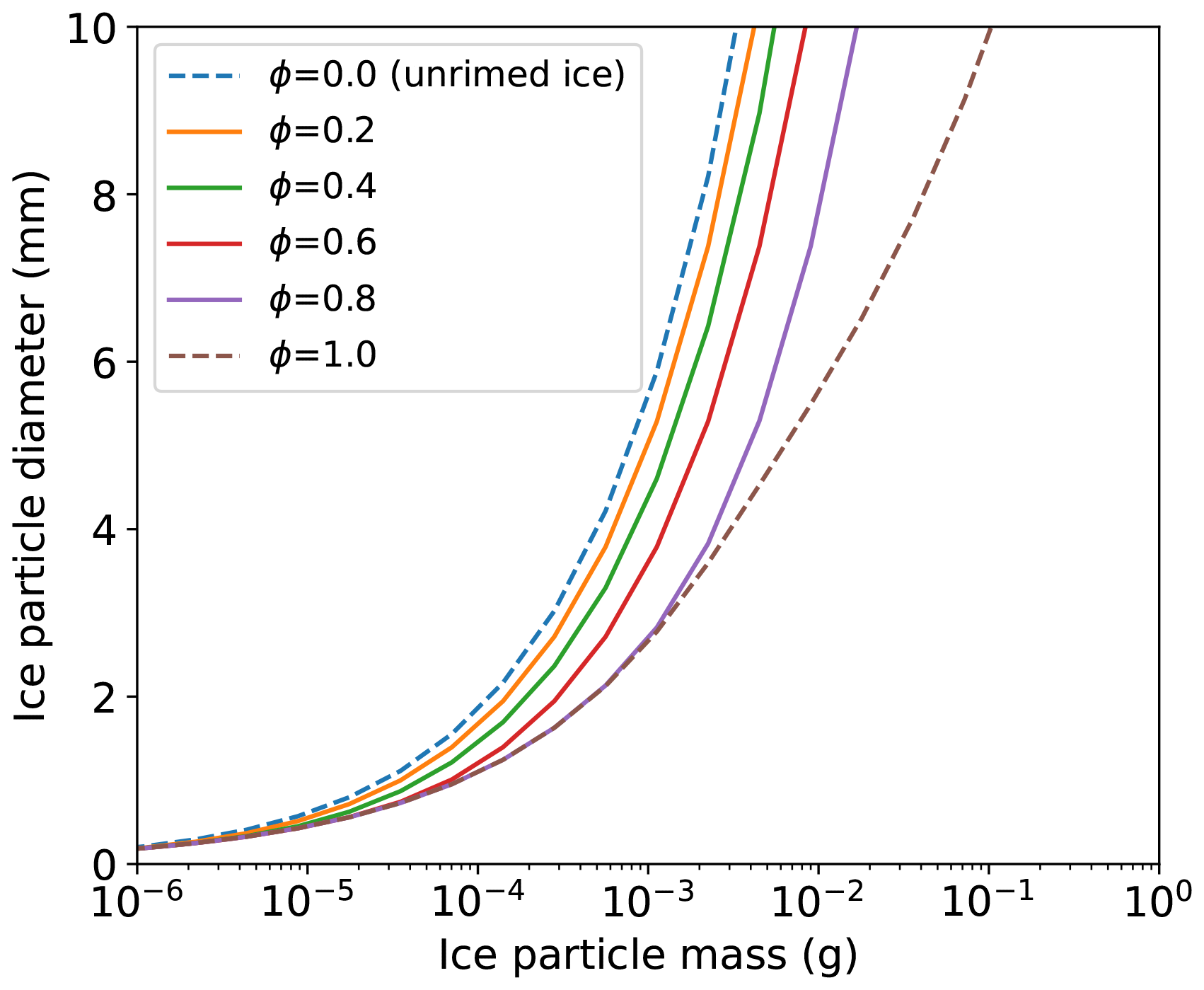
Figure 1 Mass–diameter relation of the ice particles in DESCAM depending on the rime fraction ϕ based on the “fill-in” concept of Heymsfield (1982) and Morrison and Grabowski (2010).

In DESCAM, the density of ice particles can be diagnosed from the mass–diameter relationships presented in Fig. 1, resulting in rimed particles being denser than unrimed ones. Fully rimed particles, typically classified as graupel, exhibit densities of around 0.2 g cm⁻³ for millimeter-sized particles. This density is comparable to the graupel generated in the laboratory experiments of Grzegorczyk et al. (2023) under dry growth conditions (i.e., liquid water content of 0.7 g m⁻³ at −20 °C), meaning that fully rimed particles in DESCAM correspond to low-density graupel. This density results from the graupel mass–diameter relationship adopted from Heymsfield et al. (2018) (Table 3, “Graupel and small hail”).

However, the choice of the graupel properties in this study is quite arbitrary, given the fact that graupel properties are highly variable in nature (e.g. see Heymsfield, 1978). Furthermore, the choice of the graupel properties is critical, as it can strongly influence terminal velocity, collision kernels for riming and aggregation, SIP processes, and ultimately precipitation rates. Therefore, as discussed in Sect. 5, future developments will focus on predicting ice density directly to remove the dependency on a fixed m–D relation and better represent processes such as wet growth that would leaf to much denser rimed particles.

2.3 Terminal velocity of ice particles

While the size of ice particles can change smoothly depending on their riming degree, their shape is not explicitly represented in DESCAM and is assumed to be spherical when shape is required in calculation. To calculate the terminal velocity of ice particles from their size and mass without supposing any predefined shape, a common approach relies on dimensionless numbers that describe the aerodynamics of ice particles. The Best number, X and the Reynolds number, Re were introduced by Abraham (1970) to describe the drag coefficient of a sphere and were extended by Böhm (1989) for ice particles. Based on the same considerations, different parameterizations have been proposed in the literature (Mitchell, 1996; Khvorostyanov and Curry, 2002, 2005; Mitchell and Heymsfield, 2005). The parameterization used in DESCAM is that of Heymsfield and Westbrook (2010) which provides a modification of the Best number X and Reynolds number Re defined by:

$$\begin{array}{}\text{(3)}& \mathit{Re}={\displaystyle \frac{{\mathit{\delta }}_{\mathrm{0}}^{\mathrm{2}}}{\mathrm{4}}}\left[\right(\mathrm{1}+{\displaystyle \frac{\mathrm{4}\sqrt{X}}{{\mathit{\delta }}_{\mathrm{0}}^{\mathrm{2}}\sqrt{C_{\mathrm{0}}}}}{)}^{\frac{\mathrm{1}}{\mathrm{2}}}-\mathrm{1}{]}^{\mathrm{2}}\end{array}$$

with C₀=0.35 the inviscid drag coefficient, δ₀=8.0 a dimensionless parameter and

$$\begin{array}{}\text{(4)}& X={\displaystyle \frac{{\mathit{\rho }}_{\mathrm{a}}}{{\mathit{\nu }}^{\mathrm{2}}}}{\displaystyle \frac{\mathrm{8}mg}{\mathit{\pi }{A}_{\mathrm{r}}}}\end{array}$$

with ρ_a the air density, ν the kinematic viscosity of air, m and D the ice particle mass and size and A_r the area ratio of the ice particle defined by $A_{\mathrm{r}}=\frac{A}{(\mathit{\pi }/\mathrm{4})D^{\mathrm{2}}}$ with A the projected area.

To calculate A_r, Heymsfield et al. (2002) proposed the following relation $A_{\mathrm{r}}=\mathrm{0.29}{D}^{-\mathrm{0.18}}$ based on measurements in tropical cloud anvils where ice crystals are assumed to be unrimed. For graupel particles, the area ratio is calculated from the projected area of graupel A_gr=0.625D² given in Morrison and Grabowski (2010) (cgs units). Contrary to ice particle size, the projected area and the area ratio of rimed ice crystals is not provided by the “fill-in” concept. However, since Eq. (4) depend on A_r, a smooth transition between the area ratios of unrimed and graupel particles is needed. Therefore, the area ratio of rimed ice particle is assumed to evolve linearly between those of graupel and unrimed ice particles as follows:

$$\begin{array}{}\text{(5)}& \begin{array}{rl}{A}_{\mathrm{r}}^{\mathrm{rime}}& =A_r[\mathrm{1}-({\displaystyle \frac{D_{\mathrm{gr}}-D}{D_{\mathrm{gr}}-D_{\mathit{\varphi }=\mathrm{0}}}}\left)\right]\\ & +{\displaystyle \frac{A_{\mathrm{gr}}}{(\mathit{\pi }/\mathrm{4})D^{\mathrm{2}}}}\left({\displaystyle \frac{D_{\mathrm{gr}}-D}{D_{\mathrm{gr}}-D_{\mathit{\varphi }=\mathrm{0}}}}\right).\end{array}\end{array}$$

with D the D_ϕ=0 the diameter of unrimed ice particles (cgs units).

From the previous considerations, Fig. 2 shows the terminal velocity (V) of ice particles as a function of their size and rime mass fraction (ϕ). This figure also shows the graupel terminal velocities based on the velocity–diameter (V–D) relationships of Lee et al. (2015) and Heymsfield et al. (2018) that can be compared with those calculated for DESCAM. For graupel particles smaller than 1 mm diameter, the predicted terminal velocity in DESCAM aligns closely with Lee et al. (2015), whereas for larger particles it is closer to Heymsfield et al. (2018). This could be explained by the fact that graupel can have different densities in nature while it is currently not the case in DESCAM scheme. A possible future perspective would be to predict the volume of rime, as proposed by Morrison and Milbrandt (2015a) which would allow rimed particles to have different densities and consequently gets rid of the fixed mass–diameter relation of graupel particles.

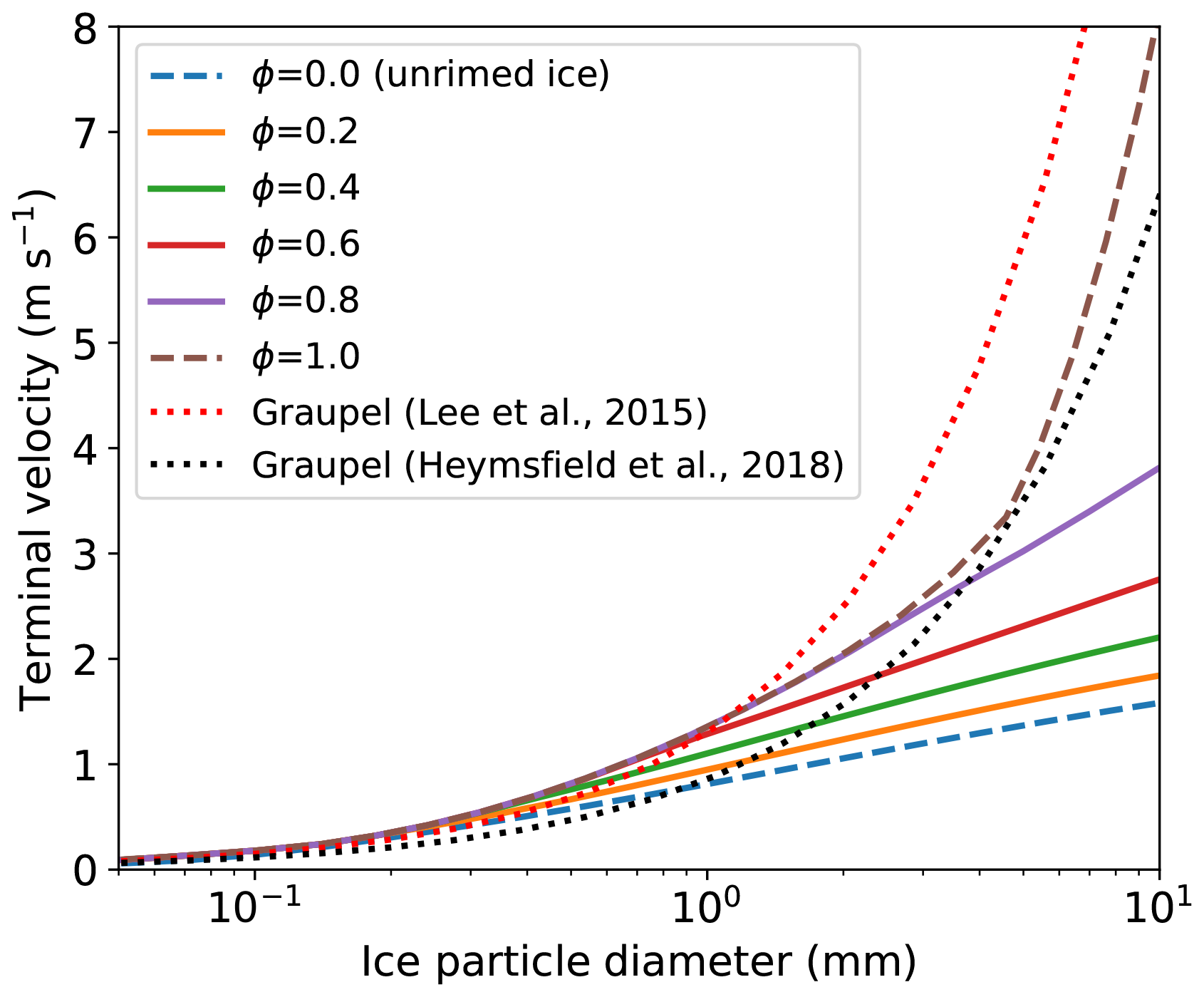
Figure 2 Terminal velocity of ice particles in DESCAM as a function of rime fraction ϕ, based on Heymsfield and Westbrook (2010) study. Dotted lines represent the graupel velocity–diameter (V–D) relationships from Lee et al. (2015) and Heymsfield et al. (2018).

2.4 Riming collision kernels

To represent the riming process in models, a key parameter is the collision kernels that quantify the rate at which two ice hydrometeors collide per unit time and volume. From the mass, size and terminal velocity of the ice particles presented in Figs. 1 and 2, the collision kernels for a drop of mass m₁ and an ice particle of mass m₂ with rime fraction ϕ are defined by:

$$\begin{array}{}\text{(6)}& K(m_{\mathrm{1}},m_{\mathrm{2}},\mathit{\varphi })={\displaystyle \frac{\mathit{\pi }}{\mathrm{4}}}(D_{\mathrm{1}}+D_{\mathrm{2}}{)}^{\mathrm{2}}|V_{\mathrm{1}}-V_{\mathrm{2}}\left|E_{\mathrm{c}}\right(m_{\mathrm{1}},m_{\mathrm{2}},\mathit{\varphi }).\end{array}$$

with V₁ and V₂ the terminal velocity of liquid drop (derived from Beard, 1976) and ice particles, respectively. E_c is the collision efficiency of riming which depends on the particles properties. For unrimed ice particles collecting liquid drops (V₂>V₁), E_c is derived from Wang and Ji (2000), while for graupel particles it follows the study of Cober and List (1993). For large liquid drops collecting ice particles (V₁>V₂), the collision efficiencies are calculated from Lew et al. (1985). Therefore, for partly rimed particles, E_c is interpolated according to the particle size as done for A_r in Eq. (5).

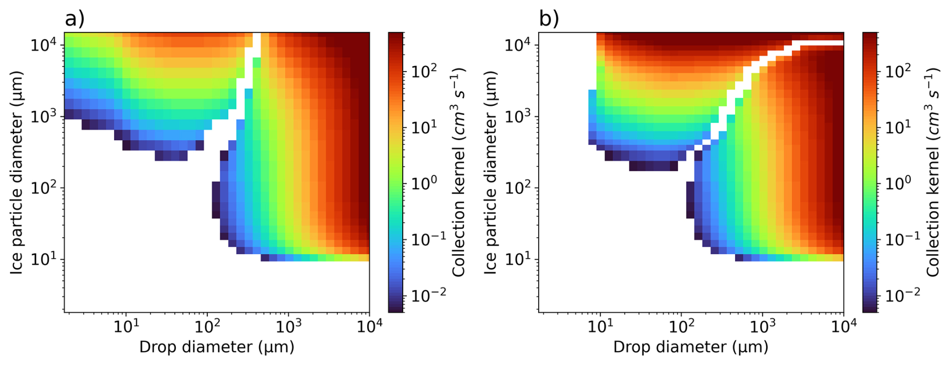
The collision kernels are presented in Fig. 3a and b for unrimed and graupel particles. In both cases, the onset of riming occurs from drop or ice particles of around 100–200 µm diameter, as found by Lew et al. (1985) and Wang and Ji (2000). Figure 3a shows an asymmetry in collision kernels due to the fact that drops fall faster than unrimed ice particles. In contrast, Fig. 3b shows a reduced asymmetry (except for large particles), as graupel particles have terminal velocities closer to those of liquid drops. This difference in terminal velocity also results in higher values of collision kernels for graupel compared to unrimed ice particles.

Figure 3 Riming collision kernels between liquid drops and ice particles, calculated using Eq. (6), that are implemented in DESCAM. Panel (a) shows the kernels for unrimed ice crystals and (b) presents those of graupel particles.

2.5 Aggregation collision kernels

Aggregation of ice particles is treated similarly to Eq. (6), taking into account the effects of rime on particle size and terminal velocity. As presented in a previous study (Grzegorczyk et al., 2025a), the collection efficiency E_c for aggregation combines the collision efficiency, determined following the theoretical work of Böhm (1992), and the sticking efficiency (E_s), based on the studies of Connolly et al. (2012) and Karrer et al. (2021).

For both unrimed and rimed particles at temperatures warmer than −5 °C, as proposed in Karrer et al. (2021), E_s is assumed to increase linearly toward 1 as the temperature approaches 0 °C, reflecting the role of the sintering mechanisms due to the presence of a quasi-liquid layer on ice surfaces.

At temperatures below −5 °C, $E_{\mathrm{s}}^{\mathrm{unrimed}}$ follows the values reported by Connolly et al. (2012), reaching a maximum of 0.6 at −15 °C due to the interlocking of dendritic branches. We suppose that riming can reduce E_s near −15 °C because droplets may fill dendritic branches and limit interlocking. Accordingly, the sticking efficiency of fully rimed crystals at −15 °C is set to 0.15, corresponding to the average of the values reported at −10 and −20 °C by Connolly et al. (2012). The overall sticking efficiency can be expressed as a weighted average based on the rime fraction:

$$\begin{array}{}\text{(7)}& E_{\mathrm{s}}(T,\mathit{\varphi })=(\mathrm{1}-\mathit{\varphi })E_{\mathrm{s}}^{\mathrm{unrimed}}+\mathit{\varphi }{E}_{\mathrm{s}}^{\mathrm{rimed}}\end{array}$$

It should be noted that the representation of aggregation and thus the assumptions made here regarding the effects of riming remains uncertain, as sticking efficiency has been investigated in a limited number of studies.

2.6 Budget equation for the rime mass distribution

The implementation of the rime mass distribution follows the same concepts and methodology as the track of aerosol mass inside ice particles and droplets developed and described by Flossmann and Wobrock (2010). The newly predicted rime mass distribution, is affected by various dynamical and microphysical processes:

$$\begin{array}{}\text{(8)}& \begin{array}{rl}{\displaystyle \frac{\partial g_{\mathrm{r}}\left(m\right)}{\partial t}}& =({\displaystyle \frac{\partial g_{\mathrm{r}}\left(m\right)}{\partial t}}{)}_{\mathrm{dyn}}+({\displaystyle \frac{\partial g_{\mathrm{r}}\left(m\right)}{\partial t}}{)}_{\mathrm{nucl}}\\ & +({\displaystyle \frac{\partial g_{\mathrm{r}}\left(m\right)}{\partial t}}{)}_{\mathrm{rim}}+({\displaystyle \frac{\partial g_{\mathrm{r}}\left(m\right)}{\partial t}}{)}_{\mathrm{agg}/\mathrm{brk}}\\ & +({\displaystyle \frac{\partial g_{\mathrm{r}}\left(m\right)}{\partial t}}{)}_{\mathrm{dep}}+({\displaystyle \frac{\partial g_{\mathrm{r}}\left(m\right)}{\partial t}}{)}_{\mathrm{sub}}\\ & +({\displaystyle \frac{\partial g_{\mathrm{r}}\left(m\right)}{\partial t}}{)}_{\mathrm{melt}}\end{array}\end{array}$$

The left-hand term of Eq. (8) represents the total variation in rime mass g_r(m) for an ice particle of mass m, due to the the sources and sinks generated by the microphysical processes. The effect of transport and sedimentation of ice particles is expressed by the first term on the right-hand side of Eq. (8). As expressed by the second term on the right-hand side of Eq. (8), we also consider frozen drops generated by nucleation following Hiron and Flossmann (2015) method (i.e., condensation, immersion freezing, and homogeneous nucleation) as a source of rime. The third term represents the variation in rime mass caused by the collision of ice particles with liquid drops and is expressed as:

$$\begin{array}{}\text{(9)}& \begin{array}{rl}({\displaystyle \frac{\partial g_{\mathrm{r}}\left(m\right)}{\partial t}}{)}_{\mathrm{rim}}& =g_{\mathrm{d}}\left(m_{\mathrm{1}}\right)g_{\mathrm{i}}\left(m_{\mathrm{2}}\right){\displaystyle \frac{K(m_{\mathrm{1}},m_{\mathrm{2}},\mathit{\varphi })}{m_{\mathrm{2}}}}\\ & +g_{\mathrm{d}}\left(m_{\mathrm{1}}\right)g_{\mathrm{r}}\left(m_{\mathrm{2}}\right){\displaystyle \frac{K(m_{\mathrm{1}},m_{\mathrm{2}},\mathit{\varphi })}{m_{\mathrm{1}}}}.\end{array}\end{array}$$

with g_i the total ice mass distribution, g_d the liquid drop mass distribution and $K(m_{\mathrm{1}},m_{\mathrm{1}},\mathit{\varphi })$ the riming collision kernel presented in Fig. 3. The first term of the right-hand part of Eq. (9) expresses the gain of newly formed rime mass for an ice particle of mass m due to the collision between drops of mass m₁ with ice particles of mass m₂ having a rime fraction ϕ. Furthermore, as ice crystals grow by riming, their total mass is transferred to larger bins. Consequently, the initial rime mass of the colliding ice particle (m₂) must also be redistributed into larger bins. This effect is taken into account by the second term of Eq. (9), which considers the transport of pre-existing rime mass. Since the mass gained from the collision (m₁,m₂) does not necessarily fit the defined mass bin m, the redistribution method of Bott (1998) for the stochastic collection equation is applied.

Although aggregation does not change the total rime mass, it can redistribute it across different bins, depending on the combined rime masses of the colliding particles (fourth right-hand part term of Eq. 8). The transport of rime due to the aggregation of two ice particles is treated similarly to riming (second term of the righ-hand part of Eq. 9). Furthermore, when ice particles do not stick but break, the rime mass fraction of the parent particle is kept constant. Additionally, the loss of rime mass due to fragmentation is considered.

Similarly to riming, when a particle gains mass through vapor deposition (fifth term of Eq. 8), it is necessary to transfer the rime mass of the initial particle into larger bins. Therefore, the gain or loss of rime mass is set to be proportional to the number of ice particles growing (or shrinking) to larger (or smaller) bin during vapor growth (or sublimation), as is detailed in Appendix A.

The sixth term of Eq. (8) represents the loss of rime mass through sublimation. Since there is no information about the surface properties of the ice particles (i.e. consisting of rime or vapor-grown ice), we assume that the particle rime fraction ϕ remains constant during sublimation. As a result, the rime mass decreases in the same proportions as for the total ice mass. Finally, the last term of Eq. (8) expresses the sink of rime mass due to melting of ice particle (which is set to occur instantaneously, contrary to Planche et al., 2014).

To ensure the correct transport of rime mass through the binned distribution, numerical tests were conducted by using predefined rime mass distributions for each process included in Eq. (8) (with transport of sedimentation turn off). Similar tests of rime transport during depositional growth, aggregation and riming are presented in Morrison and Grabowski (2010) (their Figs. 1, 2 and 4).

3 Simulation cases

3.1 Idealized squall line system

The first numerical experiment of this study examines the consequences of the predicted rime implementation in DESCAM for a large mesoscale convective system similar to the squall line that occurred on 20 June 2007 in Oklahoma and Kansas. A semi-idealized setup with 3D dynamics was applied as presented for an intercomparison study as part of the 2012 Eighth International Cloud Modeling Workshop (Muhlbauer et al., 2013). A detailed description of the model set-up and results of this intercomparison study are presented in Morrison and Milbrandt (2015a, called hereafter MO15) and Morrison et al. (2015).

We used the environmental temperature and moisture profiles described in Morrison et al. (2009) and Weisman and Klemp (1982, 1984) instead of the sounding given in MO15. The convective available potential energy (CAPE = 2300 J kg⁻¹) is less pronounced than the one in MO15. This limits the extension of the cloud system in z and x direction compared to MO15 and helps to reduce the numerical cost of the simulations. The model domain is set to 382 × 128 points. The grid spacing is 1 km horizontally and 250 m vertically. The melting level is located at a height of 4 km and the model top at 25 km. The horizontal wind profile has a shear of 0.0048 s⁻¹ in the lowest 2.5 km altitude and zero shear above. The mean wind above 2.5 km is zero, which helps to keep the squall line near the center of the domain. A Rayleigh damper with damping coefficient of 0.003 s⁻¹ is applied to the top 5 km. The upper and lower boundaries are free slip and rigid. Lateral boundary conditions are open.

As in MO15, convection is initiated in an uniform thermodynamic environment by applying a force to the u wind during the first hour of integration, providing convergence at low levels. The forcing term is prescribed as

$$\begin{array}{}\text{(10)}& {\displaystyle \frac{\partial u}{\partial t}}=\mathit{\alpha }\mathit{\gamma }\cos \left[{\displaystyle \frac{\mathit{\pi }(x-x_{\mathrm{c}})}{\mathrm{2}{x}_{\mathrm{r}}}}\right]\times \left[\cosh \right({\displaystyle \frac{\mathrm{2.5}z}{z_{\mathrm{r}}}}){]}^{-\mathrm{2}}\end{array}$$

where γ=1 during the first 55 min of integration and then decreases linearly to γ=0 at 60 min. In our study, x_c=192 km is the center of the forcing, x_r=10 km, z is the height (in km), z_r=10 km and α=0.1 m s⁻² is the maximum forcing amplitude, and t the time in s.

To initiate 3D motion, random fluctuations perturbation of the potential temperature field are applied in a 25 km wide region with a maximum amplitude of ±0.05 K located next to the center x_c.

3.2 Heavy snowfall event during ICE-POP 2018

The second case study evaluates the relevance of the DESCAM implementations, by comparing the model results with ground-based field observations. It focuses on the snowfall event that occurred between 7 and 9 March 2018, during the passage of a low-pressure system over the Korean Peninsula during the ICE-POP 2018 campaign. This event is categorized as “warm low” according to Kim et al. (2021), following the synoptic classification of Jeoung et al. (2020). The “warm low” system forms over the southwestern part of the Korean Peninsula due to the abundant moisture supplies from the East China Sea. This moisture leads to the development of precipitating cloud systems moving across the peninsula and producing heavy snowfall.

After the passage of the low pressure deep system, the wind in the upper layer shifts from southwest to northeast, bringing in dry air. Consequently, a shallower cloud system forms exclusively in the lower layer. This system is mainly influenced by moisture from the East Sea, driven by sea-air interactions and orographic lifting along the eastern mountainous coastal region. More details on this type of cloud system can be found in Kim et al. (2021).

3.2.1 Observations

Observations were conducted at several measurement supersites equipped with ground-based microphysical probes, wind profilers, radars, and both fixed and mobile radiosounding stations. An overview of the instrumentation of the ICE-POP 2018 campaign can be found in Kim et al. (2021), Gehring et al. (2021, 2020b), and Tsai et al. (2022). The present study mainly uses the instrumentation of the MHS (Mayhills supersite; 37.6652° N, 128.6996° E; 789 m altitude) station. This site includes a vertically pointing X-band radar and a W-band cloud Doppler radar, both providing radar reflectivity. A OTT Pluvio² rain gauge is used to measure the rainfall accumulation and intensity and an OTT Parsivel² disdrometer (Tokay et al., 2014) is used to determine the dominant type of precipitation (rain or snow). The Particle Imaging Package (PIP, Newman et al., 2009; Pettersen et al., 2020) probe provides the size distribution of ice particles from 0.1 to 26 mm diameter. Complementary, a multi-angle snowflake camera (MASC, Garrett et al., 2012) is used to obtain the morphological properties of the ice particles following Praz et al. (2017) method, providing a rime index (ranging from 0 to 1) and a classification in 6 hydrometeors types. In addition, three other disdrometers and rain gauges, deployed at YPO (Yongpyong Observatory; 37.6433° N, 128.6705° E; 772 m altitude), BKC (Bokwang-ri Community Center; 37.7381° N, 128.8058° E; 175 m altitude), and GWU (37.7709° N, 128.8669° E; 36 m altitude) are used in this study to provide the precipitation properties previously mentioned.

Figure 4b shows the locations of the measurement sites mentioned previously, within the third (most refined) domain of DESCAM model. As visible from the orography cross section in Fig. 4c, the YPO and MHS sites are located in mountainous regions while BKC and GWU are close to the coast (i.e. at lower altitudes).

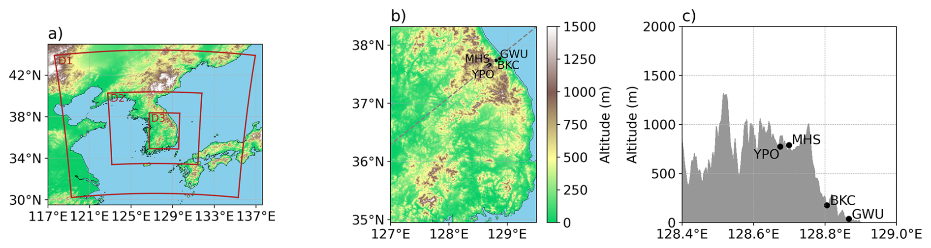
Figure 4 (a) Nested model domains of DESCAM considered for the numerical experiments with 8 km (D1), 4 km (D2) and 1 km (D3) horizontal resolution. (b) Location of the measurement sites of the ICE-POP 2018 campaign indicated in the innermost model domain. (c) Orography and positions of the measurement sites along the transect indicated in (b).

3.2.2 Numerical setup

In this study, the bin microphysics scheme DESCAM (see Sect. 2.1 and 2.2 for more details) included in the 3D dynamical frame of Clark et al. (1996) and Clark (2003) is used. The numerical experiment consists of three nested domains shown in Fig. 4a, composed of 193 × 193, 193 × 193 and 258 × 386 grid points corresponding to horizontal resolutions of 8, 4 and 1 km, similar to the setup of Park et al. (2024). The vertical grid is non-equidistant, with 82 vertical levels ranging from Δz=40 m at ground level and Δz=230 m at 9 km. The simulations are run for two days from 7 March 2018 at 00:00 UTC to 9 March 2018 at 00:00 UTC with a time step Δt=4 s. The initial and boundary conditions of DESCAM are taken from ERA 5 ECMWF reanalysis (Hersbach et al., 2020). The aerosol particle size distribution is derived from the measurements of Yum et al. (2007) at Jeju Island (during March–April) and Park et al. (2021) at Baengnyeong Island, for air masses coming from the East China sea (classified as Type II and III in the aforementioned studies) which is where the cloud system forms. Therefore, the total aerosol particle concentration is set to 4500 cm⁻³ at ground and is assumed to decrease exponentially to 1500 cm⁻³ for altitudes above 3 km. We assumed that aerosol particles are composed of ammonium sulfate, as for this case study, the air masses mainly originated from the ocean (the East Sea for the shallow system and the China Sea for the deep system), although some influence from more polluted conditions cannot be excluded.

Two simulations were conducted for each case study (i.e. squall line and ICE-POP): the “CTRL” simulation which disables the predicted rime scheme and follows the original configuration (i.e. Control version) of DESCAM before the new developments and the second one mentioned as “pRIME” simulation, which includes the recent implementation of the predicted rime described in Sect. 2.1.

4 Results

4.1 Idealized squall line system

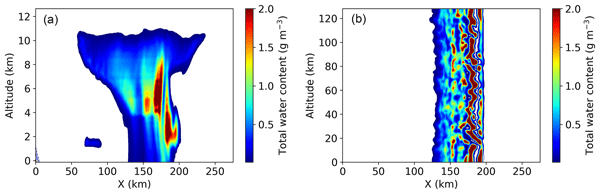
Figure 5 presents a vertical and an horizontal cross section of total water content (TWC) at 5 km altitude from the pRIME simulation, illustrating the extent of the squall line at 2.5 h of integration. This time was selected for the present analysis because the system remains quasi-steady between 2 and 4 h, while differences in precipitation pattern arise after 2.5 h indicate diverging cloud development. The squall line reaches up to 11.5 km altitude, and its anvil extends about 200 km in the x direction (Fig. 5a). The horizontal cross section (Fig. 5b) shows relatively continuous values along the y axis, which will be therefore averaged in the subsequent analyses.

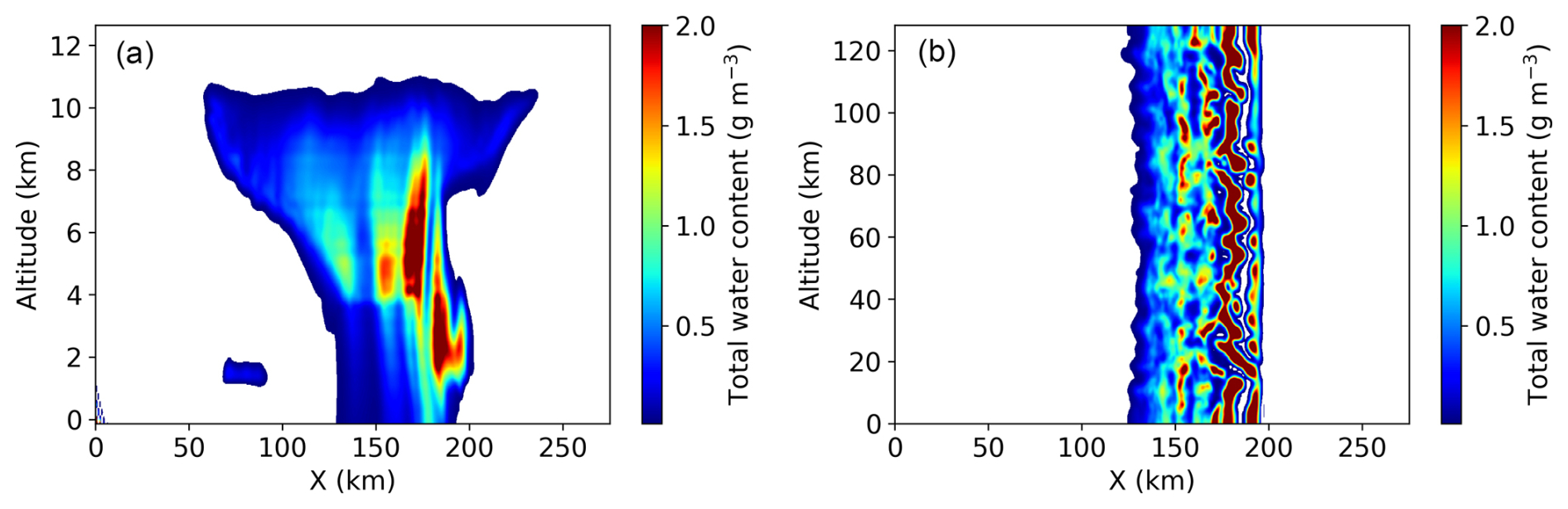
Figure 5 Total water content (TWC) of the squall line from the pRIME simulation at 2.5 h (only values >0.01 g m⁻³ are shown). (a) y-averaged vertical cross section and (b) horizontal cross section at 5 km altitude.

To evaluate the effect of the new predicted rime scheme, averaged vertical profiles of the squall line system are presented by Fig. 6 at 2.5 h.

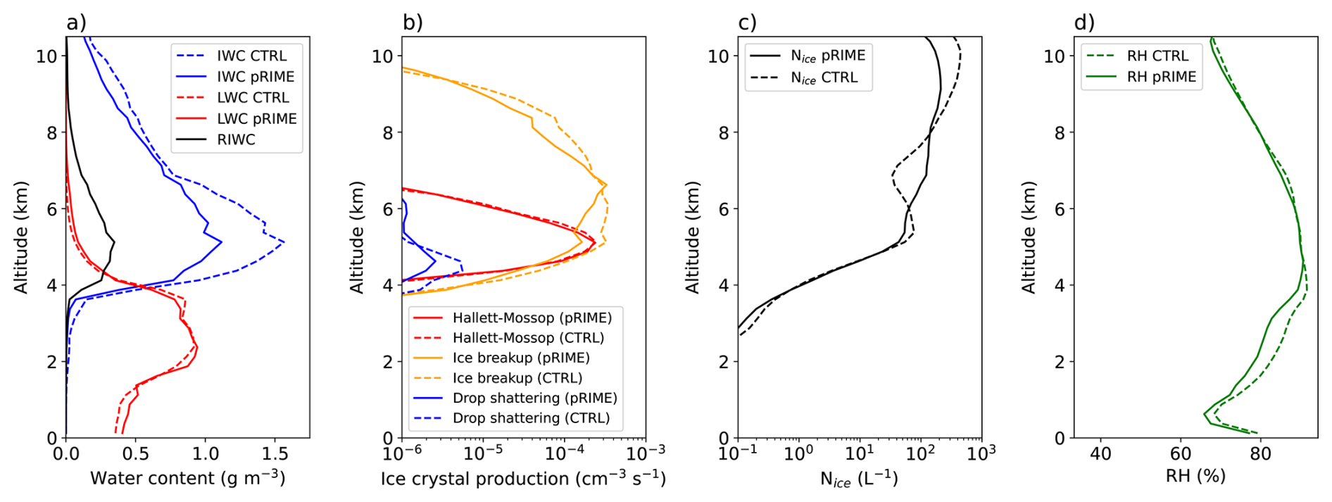
Figure 6 Vertical averaged profiles (for TWC > 0.01 g m⁻³ at 2.5 h) of cloud contents (a), rate of SIP processes (b), ice particle number concentration (c) as well relative humidity (d).

First, Fig. 6a shows that the ice water content (IWC) in the pRIME simulation is reduced by about a factor of two compared to CTRL (note that rime mass (RIWC) is included in the IWC) while the liquid water content (LWC) in pRIME is slightly higher below the melting layer (∼4 km). This slight mass increase in the warm phase of the cloud (below the melting layer) results from higher fall velocities associated with the explicit prediction of rime. Indeed, Fig. 6a shows that for the pRIME simulation, the mean Rime Ice Water Content (RIWC) reaches up to 0.4 g m⁻³, which represents approximately 40 % of the IWC below 7 km.

In Fig. 6b, the production rate of ice particles from SIP processes shows that the ice collision breakup mechanism is stronger in the pRIME simulation, due to higher terminal fall velocities of rimed particles. The Hallett-Mossop process rate remains unchanged, while the drop shattering mechanism appears to decrease. Although SIP produces more ice particles in the pRIME simulation due to stronger ice breakup, the average ice particle number concentration in Fig. 6c is overall lower in pRIME, likely because faster sedimentation due to riming reduces their persistence within the cloud. An exception occurs near 7 km (i.e. −15 °C) where N_ice in the pRIME simulation is higher due to the lower sticking efficiency of rimed particles (see Sect. 2.5 about aggregation).

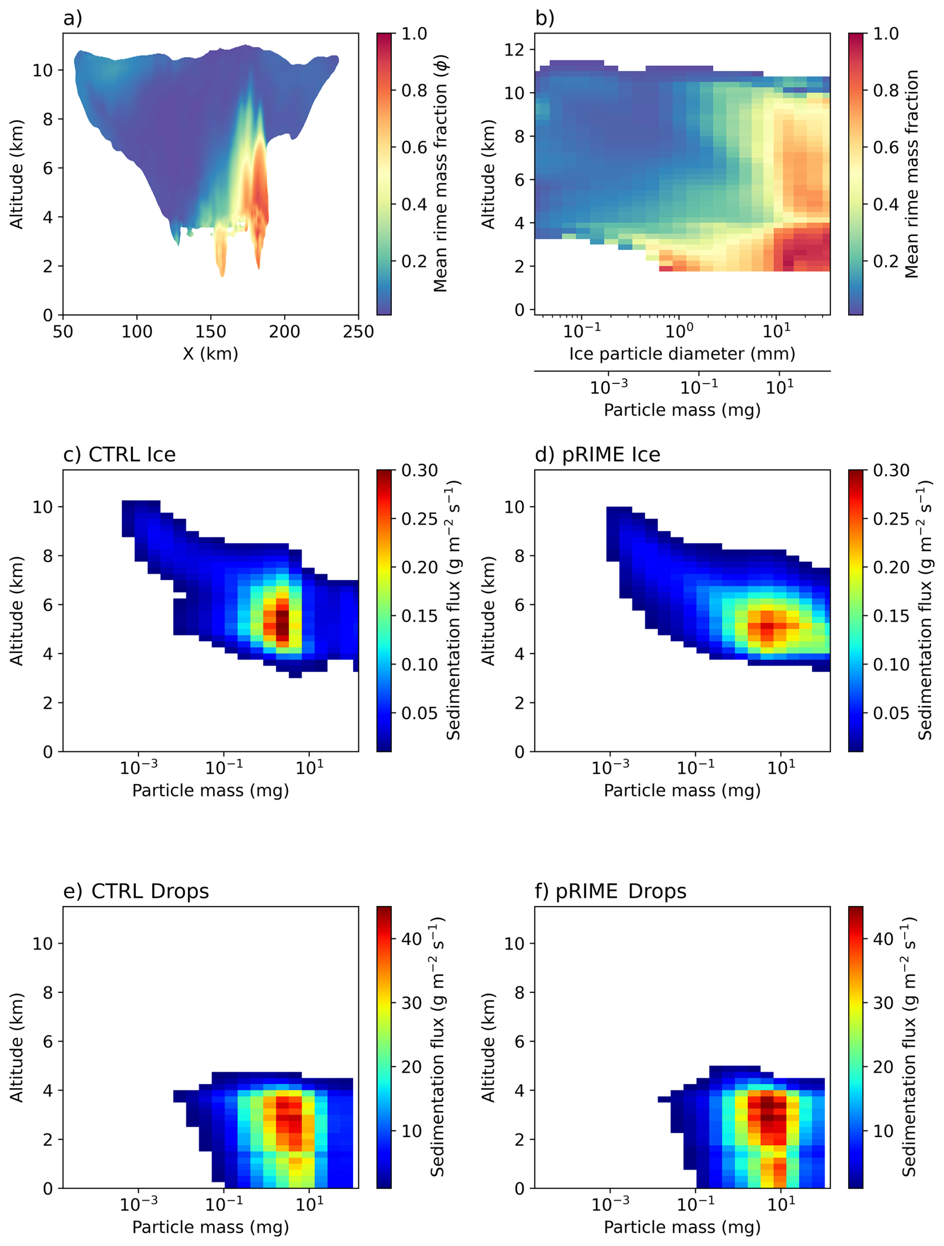
Figure 7 Vertical cross section (y-direction averaged) of the mean rime mass fraction ϕ (a), mean rime mass fraction as function of the particle size and altitude (b). Sedimentation flux of ice particle as function of ice particle size or mass and altitude for the CTRL (c) and pRIME simulation (d). Sedimentation flux of drops as function of their size and altitude for the pRIME (c) and CTRL simulation (d). All panels are averaged for TWC > 0.01 g m⁻³ at 2.5 h.

To further analyze the rime mass implementation in DESCAM, Fig. 7a shows the y-averaged vertical cross section of the rime mass fraction (ϕ). It shows that for a large part of the squall line, ϕ exceeds 0.5, especially around the main convective core and up to 9 km altitude. The rime mass fraction even approaches 1 within the main convective core due to the strong presence of supercooled liquid water in this region. Furthermore, it is visible that rimed ice particles fall up to 2 km below the melting level, consistent with the results of Morrison and Milbrandt (2015b) (see their Fig. 6).

Figure 7b illustrates how the rimed ice is distributed across different ice particle sizes and masses (i.e. bins). At all altitudes, rime fraction increases with particle size (or mass), exceeding 50 % for particles larger than 1 mm. This can be explained by the fact that large ice particles have higher collision kernels, which favor riming. Below the melting level, the rime mass fraction is even more pronounced, which is consistent with the ability of such ice particles, characterized by high density and high fall speed, to remain partially solid at positive temperatures.

As the presence of rime on large ice particles increases their fall speed, Fig. 7c–d shows the sedimentation flux of ice particles as a function of their size and altitude for the CTRL and pRIME simulations. A clear increase in sedimentation flux mode is observed across 4 to 7 km altitudes for large particles in pRIME. While in CTRL (Fig. 7c), the sedimentation flux is concentrated near 5 mg (2 mm ice particles), with only weak contributions from particles larger than 10 mg, in pRIME (Fig. 7d) the peak shifts toward 10 mg (7 mm ice particles) with the sedimentation flux becoming significant for ice particles above this value. Indeed, the presence of larger (i.e. more massive) ice particle in pRIME simulation is clearly visible in the mass size distribution (see Fig. B1a in Appendix B).

Similarly, Fig. 7e–f show the sedimentation flux of liquid drops. Below 4 km (T>0 °C), the flux of drops around 10 mg (2.7 mm) becomes higher in pRIME compared to CTRL. In addition, the sedimentation flux of large drops (>20 mg, 3.5 mm) also increases significantly in pRIME. This increase toward larger drops coincides with the upward shift of ice particle sedimentation flux in the ice phase (see Fig. 7d), suggesting that it results from the melting of large rimed ice particles located just above the melting layer. This is further supported by the mass distribution of ice particles above the melting layer (Fig. B1a) and of drops just below it (Fig. B1b), which present similar differences between the CTRL and pRIME simulations.

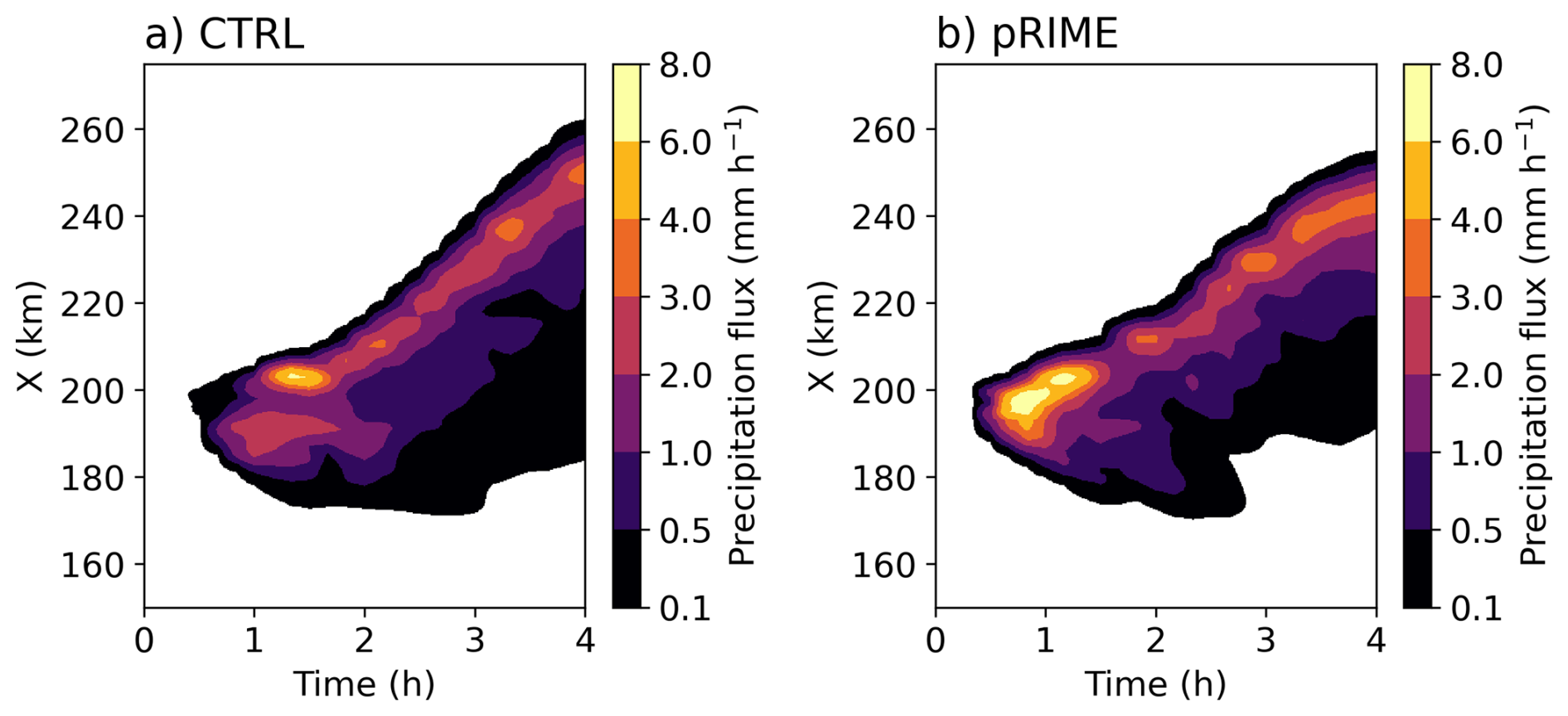
Figure 8 Temporal and spatial (y-averaged) evolution of precipitation rate larger than 0.1 mm h⁻¹ for the CTRL (a) and pRIME (b) simulations.

The effect of the explicit rime prediction on the liquid phase properties of the squall line becomes also visible in the evolution of the precipitation rate presented in Fig. 8. The pRIME simulation (Fig. 8b) exhibits stronger and earlier precipitation rates compared to the CTRL simulation (Fig. 8a). Overall, the pRIME simulation produces 15 % more precipitation than CTRL. This increase is consistent with the shift and rise of the precipitation flux toward larger drops, resulting from the melting of rimed ice particles, as shown in Fig. 7.

Furthermore, the location of the precipitation maximum intensity also shifts from 2.5 h. At 4 h, the maximum in the pRIME simulation occurs at 240 km, compared to 250 km in CTRL. This suggests that the propagation of the squall line and therefore the convective properties of the cloud system can be influenced by the rime mass prediction.

A possible explanation lies in the differences in drop size distributions (DSD) between the two simulations. Indeed, as supported by Fig. B1b–c, pRIME produces more large drops and fewer small ones, which lead to a reduction of evaporation in the cold pool (not shown here), consistent with a lower relative humidity below the melting layer in Fig. 6d. The weaker evaporation in the pRIME simulation reduces the cold pool cooling which is a key driver of squall line convection, leading to a weaker convective intensity and a more stationary cloud system as visible in Fig. 8. In contrast to that, the smaller droplets in the CTRL simulation enhance evaporation, produce larger and stronger cold pool, and consequently support more vigorous convection and faster squall-line propagation, as noted by Morrison et al. (2012). This effect observed here for the pRIME simulation was also reported by Van Weverberg et al. (2012) when including a predicted graupel category in a two-moment bulk scheme. Additionally, the influence of the drop size distribution and rimed particles on squall-line cold pool intensity has been also documented by Morrison and Milbrandt (2011).

A second factor contributing to the weaker convection of the squall line is the latent heat released within the ice phase. In the pRIME simulation, stronger sedimentation reduces the mass and number of ice particles compared to CTRL (see Fig. 6a and c), resulting in lower latent heat production from vapor deposition (not shown here). This weakens the buoyancy above 4 km and, as a feedback, can also reduce the strength of the cold pool and the propagation speed of the cloud system.

4.2 Heavy snowfall event during ICE-POP 2018

This section presents the evaluation of the CTRL and pRIME simulations against ground-based measurements for a heavy snowfall case that occurred during the ICE-POP 2018 field campaign (see Sect. 3.2).

4.2.1 Cloud system intensity and evolution

Figure 9 shows the temporal evolution of W band radar reflectivity at the MHS mountainous station, for observations in panel (a) as well as CTRL and pRIME simulations in panels (b) and (c), respectively. The modeled reflectivity is calculated using the Self-Similar Rayleigh–Gans Approximation (SSRGA) method (Hogan et al., 2017; Leinonen et al., 2017), that account for the internal structure of ice aggregates. The ice particle properties for this method follow the SSRGA-LS15-B0.2 configuration described by Tridon et al. (2019), that provides the best agreement with observed reflectivity measurements. The radar observation in Fig. 9a shows two distinct cloud systems with a deep system induced by the low pressure passage until 06:00 UTC (8 March), followed by a shallower one. The deep low pressure system produces precipitation at the surface from around 09:00 UTC, whereas in both DESCAM simulations (Fig. 9b, c) the precipitation onset is delayed until 15:00 UTC. Nevertheless, the model accurately reproduces the observed weakening of reflectivity around 18:00 UTC, suggesting that the simulation does not exhibit a systematic delay but rather fails to reproduce the early development phase of the low pressure system between 09:00 and 15:00 UTC.

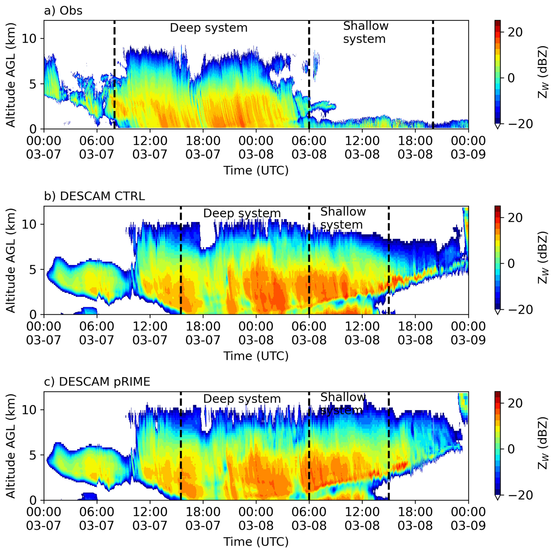
Figure 9 Time-height (above ground level) evolution of W-band radar reflectivity at the MHS station: (a) observations, (b) CTRL simulation, (c) pRIME simulation. Dashed lines indicate the limits of the different cloud systems.

Around 06:00 UTC (8 March), radar observations (Fig. 9a) show the transition of the deep low pressure system to a shallower one of around 2 km height above ground level. This system, as explained in Sect. 3.2, corresponds to the dominance of an easterly low level flow following the low pressure system, inducing orographic lifting and the formation of low level clouds. In Fig. 9b and c, although the model simulations reproduce the presence of a shallow system of 2 km height, both of them generate a second cloud layer above 2 km altitude, decoupled from the one below, that is absent in the observations. Therefore, the transition of these two cloud systems is less distinct in DESCAM than in the observations. Additionally, the shallow system starts slightly earlier in the simulation compared to the observations and consequently ends 5 h earlier, around 15:00 UTC on 8 March. The same conclusions apply for the X-band radar features also deployed at MHS (see Fig. S1 of the Supplement). In addition, the differences between the X and W band radar reflectivities are illustrated by the dual wavelength ratio reflectivity (DWR i.e. Z_X–Z_W) in Fig. S3.

To further evaluate the intensity and vertical structure of radar reflectivity, Figs. 10 and 11 present the vertical frequency distribution of the radar reflectivity for the two distinct cloud systems (the transition between the deep and shallow systems between 06:00 and 09:00 UTC is excluded in these figures). For the deep system, both DESCAM simulations (Fig. 10b and c) show high reflectivity frequencies near 10 dBZ next to the surface, matching well the intensity of the observations in Fig. 10a. Moreover, compared to the observations, the vertical decrease in reflectivity frequency is well captured by both simulations. As mentioned in Kim et al. (2021), the presence of higher reflectivity with decreasing altitude is due to the growth of snow aggregates. However, for both CTRL and pRIME, the modeled reflectivity extends to higher altitudes, reaching a maximum frequency of −12 dBZ at approximately 9 km, compared to 8 km in the observations.

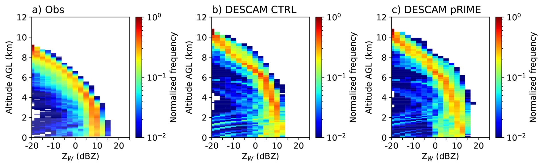
Figure 10 Frequency of W-band radar as function of the altitude above ground level for the deep cloud system (i.e. before 06:00 UTC on 8 March) presented in Fig. 9 with: (a) observations, (b) CTRL simulation and (c) pRIME simulation.

Figure 11 As Fig. 10 but for the shallow cloud system (i.e. after 09:00 UTC on 8 March).

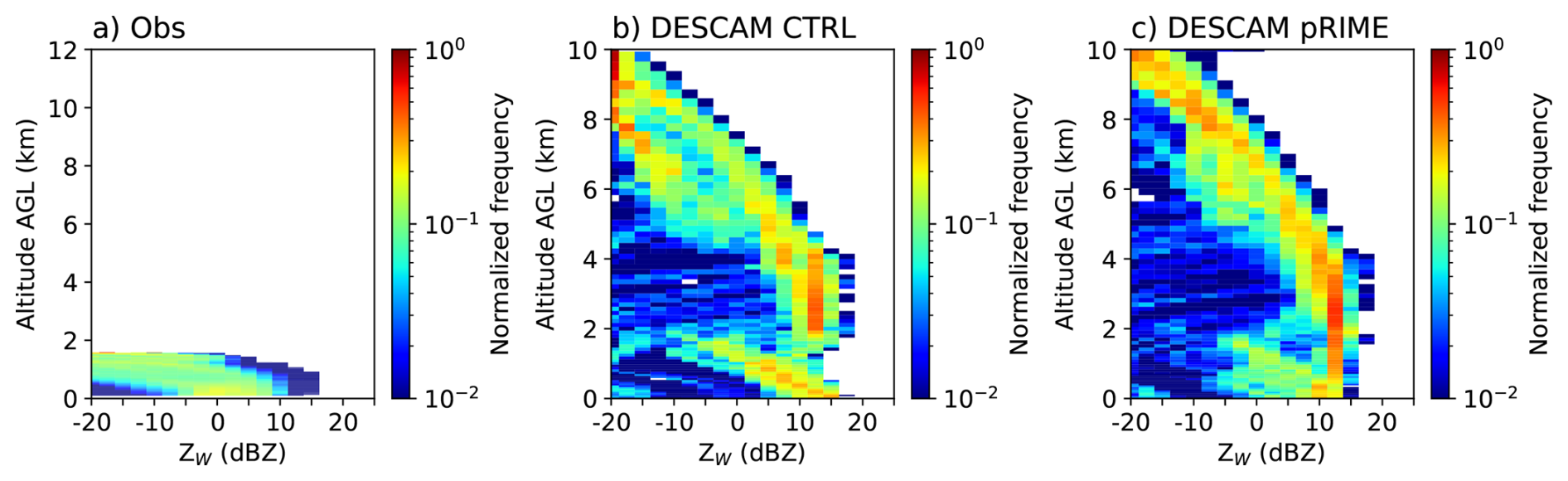
For the shallow system, radar observations in Fig. 11a display reflectivity frequencies at the surface ranging from −10 to 10 dBZ for the W band. In contrast, CTRL (Fig. 11b) exhibits higher values with a narrow surface reflectivity peak which consistently overestimates reflectivity by about +5 to +10 dB below 2 km. Compared to CTRL, the pRIME simulation (Fig. 11c) shows more variable reflectivity close to the ground (with −10 to 15 dBZ) which better matches the observations. This is due to rimed particles becoming smaller due the fill in hypothesis, reducing reflectivity while increasing variability depending on the rime mass fraction. Overall, for higher altitudes, the general vertical decrease in reflectivity up to 2 km is reasonably well captured for both simulations.

Above 2 km, Fig. 11 shows that both simulations provide high reflectivity values (from 15 dBZ at 2 km down to −10 dBZ at 8 km), similar to the structure of the earlier deep system (Fig. 10). This represents a significant discrepancy, as the observations indicate no cloud above 2 km. These differences suggest that the model may be prolonging the presence of the upper portion of the deep system, leading to an upper cloud layer above the shallow system.

To further analyze the microphysics of the cloud system, Fig. 12 shows the W-band mean Doppler velocity for the observations and CTRL and pRIME simulation. During the deep cloud system, the observed Doppler velocity near the ground is close to −1 m s⁻¹, which is accurately reproduced by both simulations, showing similar values with only some peaks reaching around −1.3 m s⁻¹. Between 4 and 6 km altitude, radar observations (Fig. 12a) show an increase in Doppler velocity up to −2 m s⁻¹. As mentioned in Gehring et al. (2020b) and Kim et al. (2021), this enhancement may be attributed to a shear layer and therefore turbulence that leads to favor aggregation and riming. This rise in Doppler velocity also coincides with temperatures near −15 °C, that favors dendritic growth and aggregation, potentially resulting in larger and faster falling ice particles. However, as the DWR, which is sensitive to ice particle size, does not significantly rise at this altitude (Fig. S2), the large Doppler velocities of Fig. 12a can be more likely attributed to riming rather than aggregation.

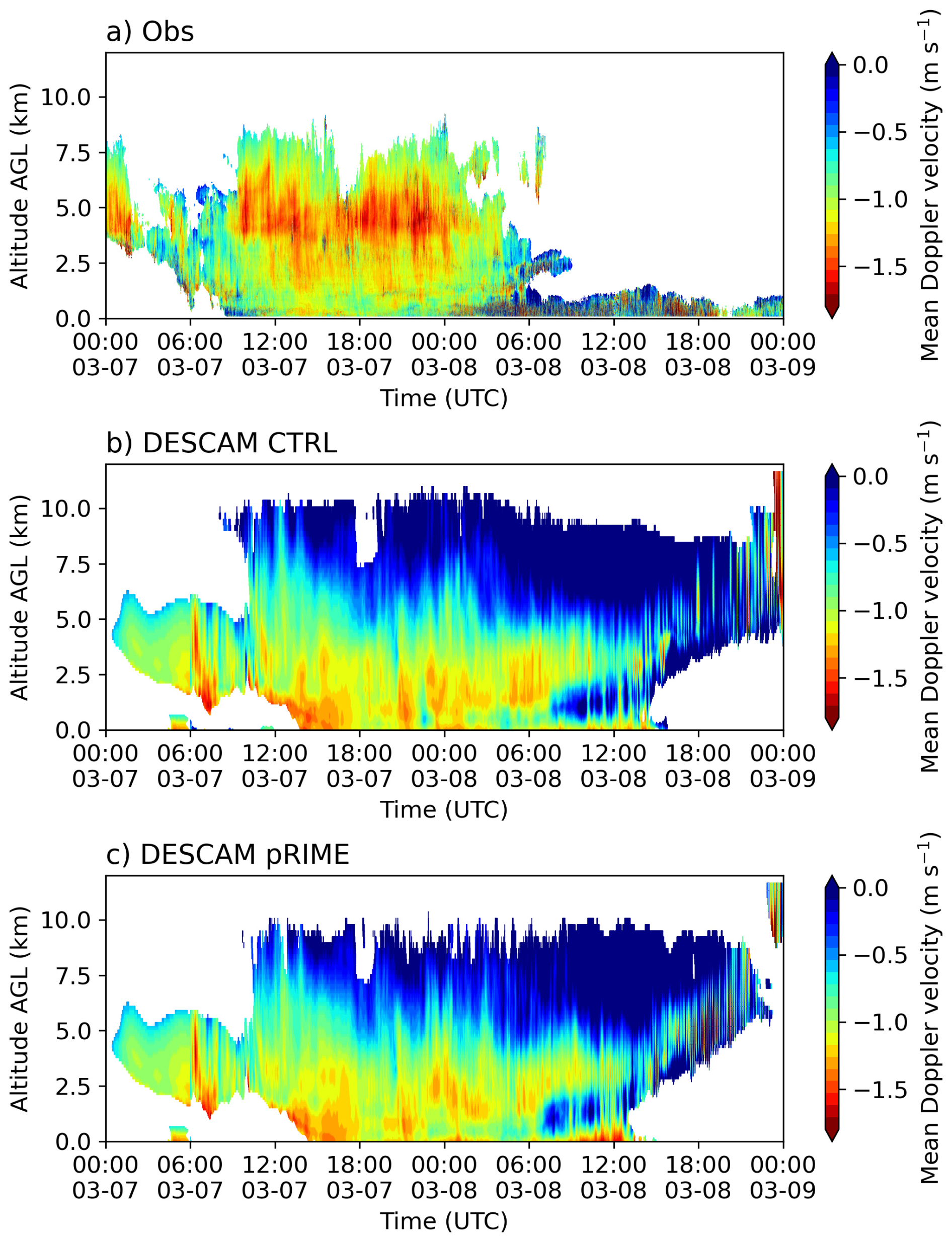
Figure 12 Mean Doppler velocity (defined positive upwards) at the MHS station for (a) W-band radar observations in and (b) CTRL simulation and (c) pRIME simulation. Data are presented for reflectivity values exceeding −20 dBZ (see Fig. 9).

For both simulations (Fig. 12b and c) the most notable increase in modeled velocity occurs near 1.5 km, within a transition layer between easterly and southwesterly airflows, where wind shear and thermal inversion are present. Close to 3.5 km, only a slight increase in Doppler velocity is provided by the model with much lower values than in the observations. Above 6 km, despite accurately representing radar reflectivity in Fig. 9, both DESCAM simulations significantly underestimate the Doppler velocity compared to the observations. This discrepancy suggests that DESCAM may generate an excessive number of small ice particles in the upper cloud layers. Indeed, while these particles can produce reflectivity intensities comparable to the observations in Fig. 9, their low terminal velocity leads to an underestimated Doppler velocity in Fig. 12.

In Fig. 12a, during the shallow cloud system and below 2 km altitude, the observed Doppler velocities show a large variability, ranging from 0 to −2 m s⁻¹, whereas the modeled Doppler velocity appears more uniform, with values around −1 m s⁻¹ in CTRL. In contrast, near the ground, pRIME exhibits stronger Doppler velocities (around −1.5 m s⁻¹), reflecting again the influence of the predicted rime in the shallow system.

Additionally, for the shallow system, in Fig. 12b and c, the modeled cloud layer above 4 km exhibits after 06:00 UTC (8 March) relatively low Doppler velocities (−1 to 0 m s⁻¹) that are associated with significant reflectivities (Fig. 9b, d). This further indicates the presence of numerous small, and slowly precipitating ice particles, similarly to the results for the upper levels of the deep system mentioned previously.

We identified that the overproduction of these small ice particles originates from a numerical artifact. Indeed, in the southwestern and northwestern corners of the outermost domain, mountainous terrain near the boundaries (Fig. 4a) appears to influence incoming air masses by generating artificial updrafts at the upper levels of the domain. These updrafts lead to an humidity enhancement at the western lateral boundary, triggering the production of a large number of ice particles by heterogeneous and homogeneous ice nucleation. It is important to note that this artificial upper cloud layer may contaminate the shallow cloud system through a seeder–feeder mechanism, potentially influencing its microphysical properties. A thorough evaluation of the microphysics of the shallow system against ICE-POP ground-based observations will be presented in the following sections.

4.2.2 Precipitation properties

The temporal evolution of accumulated precipitation at the four observation stations, based on Pluvio measurements and compared with DESCAM simulations, is shown in Fig. 13. As already observed for radar reflectivity (Fig. 9), the first phase of the cloud system is not represented by both simulations where precipitation starts at around 15:00 UTC (i.e. 3 h later than in the observations). After this delay, precipitation rate from the CTRL and pRIME simulations becomes comparable to the observations for the coastal regions (Fig. 13c, d), but remains slightly lower in the mountainous areas (Fig. 13a, b). Due to a later start, at the end of the deep system (04:00 UTC on 8 March), the accumulated precipitation in both simulations is less than half of the Pluvio measurements in mountainous areas (Fig. 13a, b) and about 5 mm lower in coastal areas (Fig. 13c, d).

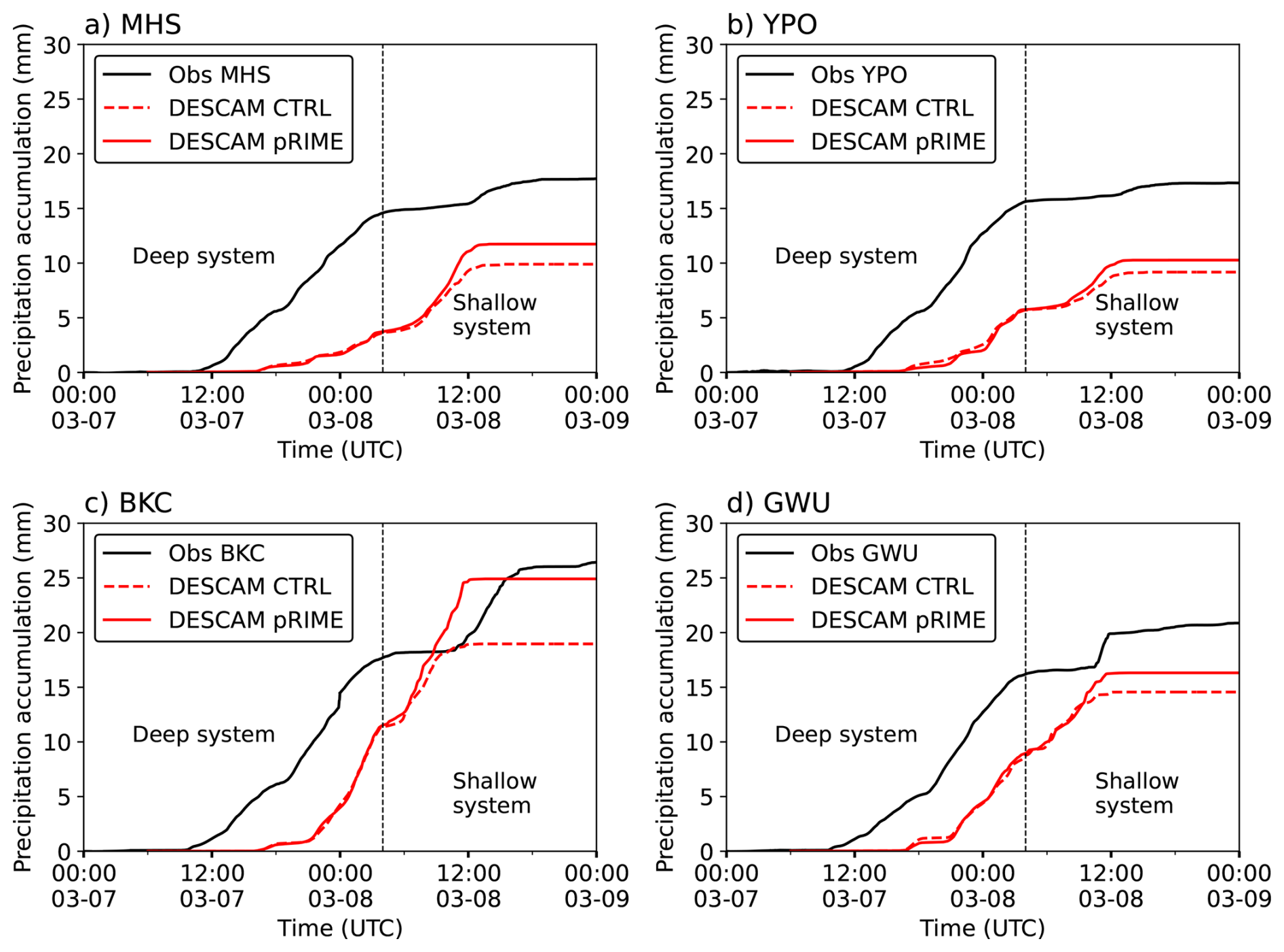
Figure 13 Temporal evolution of the precipitation accumulation at MHS, YPO, BKC, and GWU stations (see locations in Fig. 4). Black lines represent observations from the Pluvio rain gauge, while the red lines show DESCAM simulation results (a–b) for mountainous stations and (c–d) for coastal stations. Plain and dashed lines represent DESCAM results for the pRIME simulation and CTRL simulation, respectively. The black dashed lines indicate the limits of the different cloud systems.

For the shallow system, in the mountainous regions (Fig. 13a, b), DESCAM simulations lead to more intense precipitation, that starts 3 h earlier (at 09:00 UTC on 8 March) compared to the observations (at 12:00 UTC on 8 March). This aligns with the positive bias in the modeled radar reflectivity shown in Fig. 11 for the MHS station. This stronger modeled shallow system compensates the earlier underestimation of precipitation accumulation. At the coastal sites (Fig. 13c, d), pRIME simulation produces similar precipitation rate as the observed one while it starts immediately after the deep system, whereas observations show a distinct gap of 6 h between the two events.

As expected from stronger Doppler velocities and lower reflectivity during the shallow system at ground, Fig. 13 demonstrates the important role of predicted rime on precipitation formation. Turning off the predicted rime scheme in CTRL results in a reduction of precipitation at all stations, with differences between 3 and 7 mm (i.e. around 17 % to 40 %) at 00:00 UTC on 9 March. These discrepancies are most notable at the end of the deep system and during the shallow phase i.e. periods when riming is especially active. However, at the end of the pRIME simulation, DESCAM still underestimates total precipitation accumulation by about 5 mm at MHS,YPO and GWU compared to the Pluvio observations.

To further evaluate the precipitation characteristics simulated by DESCAM, Fig. 14 presents the temporal evolution of precipitation accumulation type (for >0.1 mm accumulation within 3 h) at the four observation stations. At the two mountainous stations MHS and YPO (Fig. 14a and d), Parsivel data indicate that ice particles dominate precipitation during the deep cloud system phase. Both DESCAM simulations (Fig. 14b, c, e, f) also show predominantly ice precipitation, which is consistent with the observations.

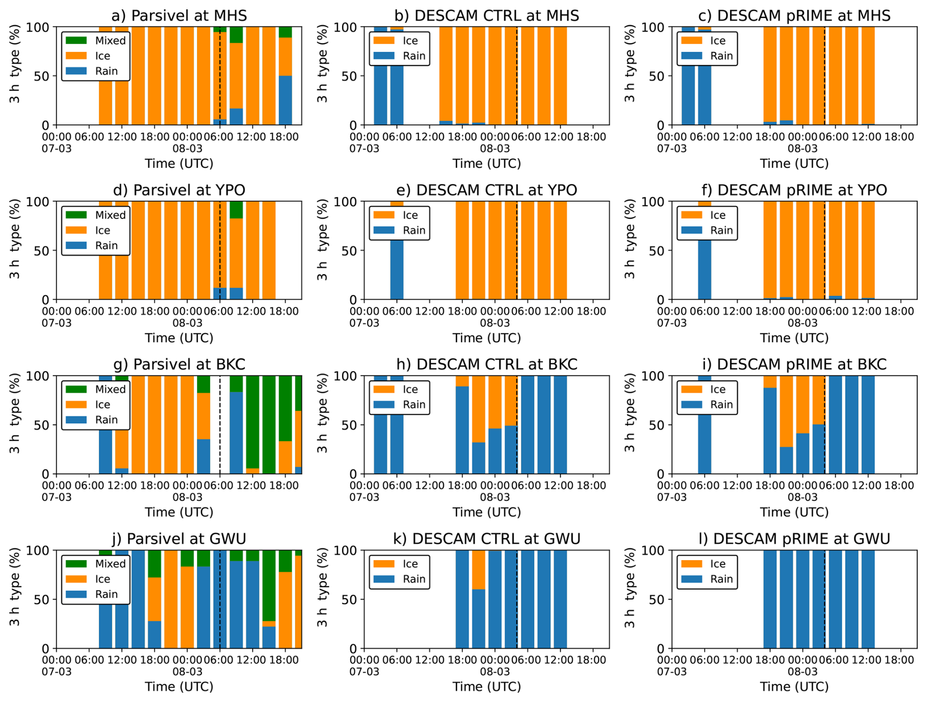
Figure 14 Temporal evolution of precipitation accumulation type (for >0.1 mm within 3 h) based at the MHS, YPO, BKC, and GWU stations observed by the Parsivel instrument (left column) and simulated by DESCAM for the CTRL (middle column) and pRIME (right column) simulation. The “mixed” particles describes melted or melting hydrometeors not identifiable as either rain or snow. The black dashed line indicate the limits between the deep and shallow cloud systems.

In contrast, for the BKC and GWU coastal stations, the model outputs (Fig. 14h, i, k, l) predominantly indicate liquid precipitation, although a minor contribution of ice particles is present at BKC but remains insufficient. The Parsivel observations in Fig. 14g and j show a transition from ice to mixed-phase (partially melted) and liquid particles during the shallow system. This suggests that DESCAM may overestimate the altitude of the melting layer in coastal regions.

The precipitation fields from CTRL and pRIME simulations (Fig. 15a, b) generally reproduce well the observed precipitation pattern and amount compared to the AWS (Automatic Weather Stations) rain product presented in Fig. 15c. Some differences still occur in the southern part of the Korean Peninsula, where the simulations show more variability, with precipitation ranging from 15 to 30 mm, while the observations are more uniform, around 25 mm, with local peaks up to 40 mm. At the ICE-POP measurement sites, both simulations show higher precipitation than the AWS-based rain product, whereas Parsivel observations (Fig. 13) report substantially larger values. Because the rain product does not include Parsivel data of ICE-POP, the analysis of precipitation in this mountainous region should rely on Parsivel measurements provided in Fig. 13.

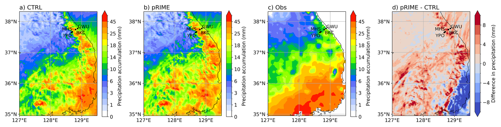
Figure 15 Precipitation accumulation (ice + rain) within the innermost domain from 7 March 00:00 to 8 March 15:00 UTC: (a) CTRL, (b) pRIME, (c) Rain accumulation product from Automatic Weather Stations (AWS) operated by the Korea Meteorological Administration (KMA) interpolated using the method of Cressman (1959) and (d) difference between pRIME in (b) and CTRL in (a).

To further assess the impact of the predicted rime mass, Fig. 15d shows the differences in precipitation accumulation between the two DESCAM simulations (pRIME-CTRL). In the southwestern part of the domain, rain accumulation rises by up to 10 mm in pRIME, which lead to produce precipitation peaks close to 40 mm, which better agree with the observations in Fig. 15c. Furthermore as visible in Fig. 15d and previously shown by Fig. 13, ice precipitation also rises by up to 10 mm in the mountainous regions of the ICE-POP campaign. Overall, the total precipitation mass in the third domain increases by approximately 7.2 % in the pRIME simulation. However, a local reduction is present in the southeastern part of the domain. This reduction could be explained by the West to East movement of the deep system combined with the higher sedimentation velocities of rimed ice particles in the CTRL simulation, that favors early precipitation in the western part of the domain. The earlier and stronger liquid precipitation of pRIME is also supported by the idealized squall line simulation results presented previously in Fig. 8.

4.2.3 Ice particles properties

Figure 16 shows the temporal evolution of ice particle size distribution at the MHS station, measured by the PIP probe (Fig. 16a) and simulated by CTRL (Fig. 16b) and pRIME (Fig. 16c), with the corresponding mean particle diameter (Fig. 16d). Both simulations produce small ice particles (<1 mm) before the onset of precipitation whereas no ice particles are detected by the PIP before 10:00 UTC. During the deep phase, both simulations (Fig. 16b, c) produce broader particle size distributions than those observed, while the mean particle diameter, fluctuating between 0.5 and 1.5 mm (Fig. 16d), remains in good agreement with the PIP measurements. In contrast, in Fig. 16d, the PIP observations show a more steady mean diameter of around 0.8 mm. The two simulations also display a bimodal distribution before 00:00 UTC (8 March) contrary to the PIP observations. These discrepancies suggest that the current representation of ice particle aggregation in DESCAM still requires further refinement.

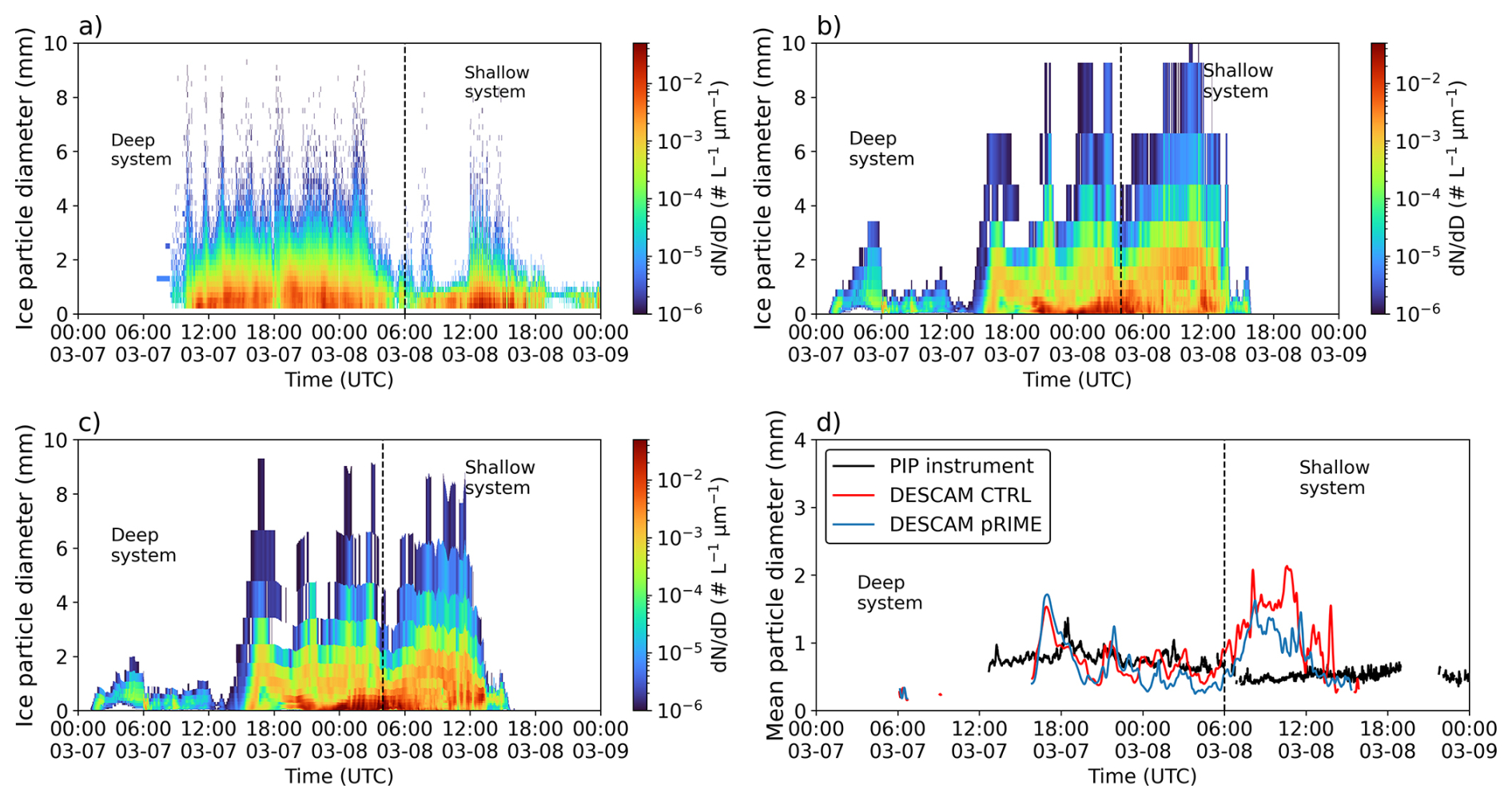
Figure 16 Temporal evolution of ground based observations of ice particle size distribution for (a) the PIP instrument at MHS, (b) CTRL simulation and (c) pRIME simulation. Panel (d) presents the number-weighted mean particle diameter (considering particles larger than 100 µm) for both simulations and the PIP observations.

In the shallow cloud phase, PIP measurements in Fig. 16d, show smaller ice particle than in the deep system with a mean diameter around 0.5 mm. While the pRIME simulation overestimates the size of the ice particles with a mean diameter around 1 mm, CTRL generates even larger particles, of about 1.5 mm before 12:00 UTC (8 March). This shows that the implementation of the predicted rime distribution helps to mitigate the overestimation of large ice particles given by CTRL.

The temporal evolution of the total number concentration of ice particles larger than 100 µm obtained from the PIP instrument and CTRL and pRIME simulations is presented in Fig. 17. During the first part of the deep cloud system (i.e. between 15:00 and 00:00 UTC on 7 March), both DESCAM simulations significantly underestimate the number of ice particles by around a factor two compared to observations. In contrast, during the second phase of the deep system (between 00:00 and 06:00 UTC on 8 March), both simulations overestimate the particle number concentration, again by a factor of two. During the shallow phase (from 06:00 UTC on 8 March), the number of ice particles in the CTRL simulation decreases after 12:00 UTC, whereas it remains relatively steady in pRIME, which appears to be more consistent with the PIP observations.

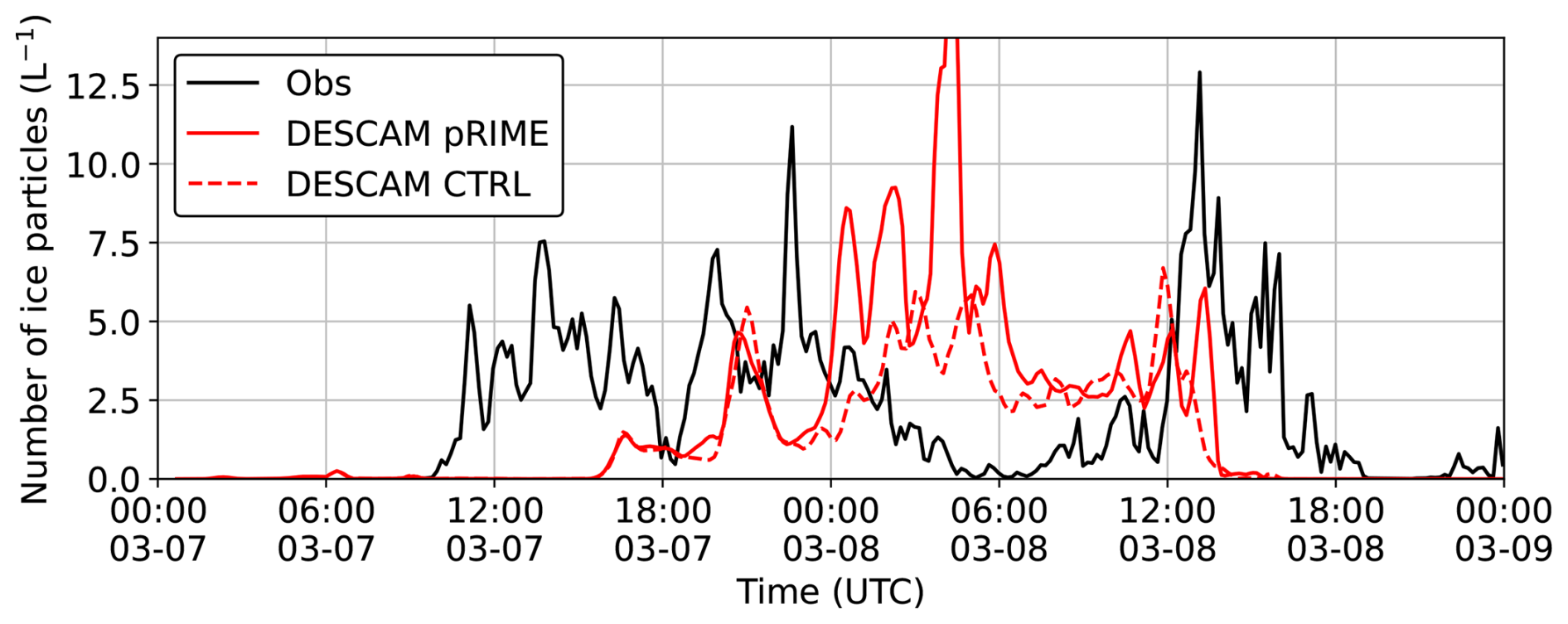
Figure 17 Temporal evolution of the number of ice particle (10 min averaged) larger than 100 µm at MHS station, observed by the PIP instrument (black line) and simulated by DESCAM, with the CTRL and pRIME simulations shown in dashed and solid red lines, respectively.

To further investigate the riming properties of ice particles, Fig. 18a shows the temporal evolution of the riming index derived from MASC images (Praz et al., 2017), as well as the simulated rime mass fraction from pRIME simulation. The rime mass fraction is defined as the ratio of rime mass to total ice mass of all particles larger than 100 µm (i.e. approximately the detection threshold of the MASC). While the riming index and rime mass fraction are different parameters, we will still compare them in order to assess the model ability to represent the evolution of rime amount in ice particles. Figure 18b displays the number of particles, from the MASC images over 10 min intervals, categorized in different hydrometeor types.

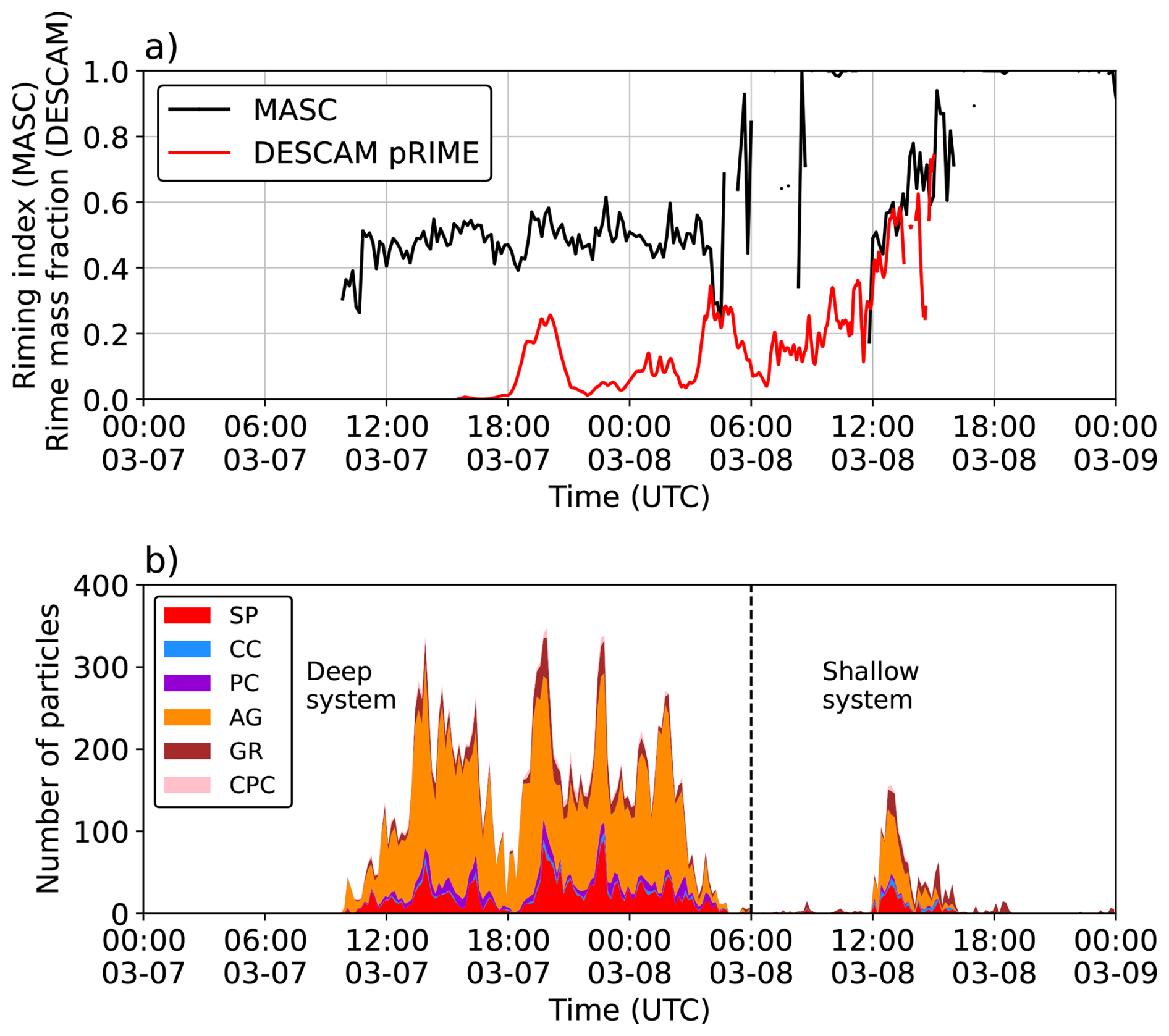
Figure 18 (a) Evolution of the rime index retrieved from MASC observations, compared to the rime mass fraction from DESCAM simulation at MHS station for >0.1 L⁻¹ ice particles. (b) Number of particles (per 10 min interval) for each hydrometeor species observed by MASC with: small particles (SP), columnar crystals (CC), planar crystals (PC), aggregates (AG), graupel (GR), and combinations of columnar and planar crystals (CPC). The rime index and hydrometeor classification are retrieved from Praz et al. (2017) method. The black dashed line indicates the limits of the different cloud systems.

During the deep system (see Fig. 18a before 06:00 UTC), the MASC riming index remains close to 0.5, along with the presence of rimed aggregates (AG) (Fig. 18b). In comparison, DESCAM gives a rime mass fraction oscillating between 0 and 0.25, suggesting a possible underestimation of rime amount during the deep phase.

At the end of the deep system, a peak is obtained for the simulated rime mass fraction around 04:00 UTC on 8 March, coinciding with peaks in the MASC riming index (from 04:00 to 09:00 UTC on 8 March). A second, more pronounced increase occurs at the end of the shallow system at 14:00 UTC on 8 March, with the MASC riming index reaching 0.9 and the simulated rime mass fraction increasing to more than 0.6. These consistent trends suggest that the predicted rime mass distribution implemented in DESCAM reproduces well the evolution of the riming properties of the ice particles.

Despite that, it remains challenging to assess whether the amount of rime mass is accurately reproduced by DESCAM. Furthermore, even if the overall properties of the shallow system agree well with ground-based observations, a potential contamination by the artificial cloud layer produced by DESCAM (see Fig. 9) on the present results can not be ruled out.

4.2.4 Riming event

To better understand the origin of the surge in rimed particle, Fig. 19 shows vertical cross sections from the pRIME simulation within the third domain. These cross-sections present the rime mass fraction with some isotherms, relative humidity (RH), and the 2D wind field as well as liquid water content (LWC) and ice water content (IWC) (along the dashed line of Fig. 4). They correspond to the deep system at 18:00 UTC on 7 March (Fig. 19a, b, c, d) and to the shallow system at 14:00 UTC on 8 March (Fig. 19e, f, g, h).

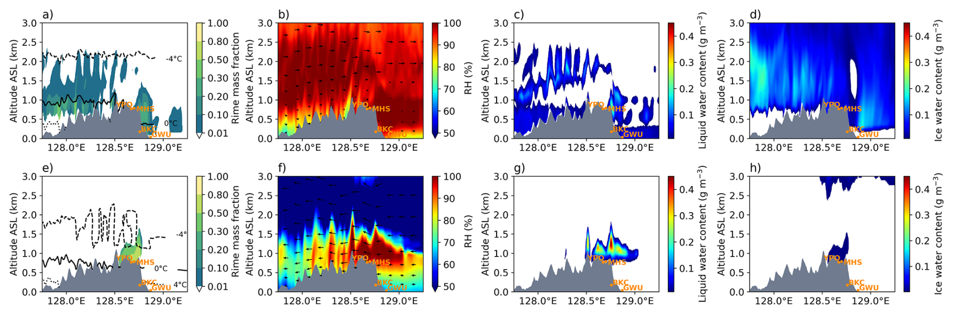
Figure 19 Vertical cross sections from pRIME simulation (along the dashed line in Fig. 4, passing through the measurement sites) within the innermost domain for the deep system at 18:00 UTC on 7 March (top row) and shallow system at 14:00 UTC on 8 March (bottom row). Panels (a), (e) show the rime mass fraction with isotherms, (b), (f) relative humidity and 2D wind field, (c), (g) liquid water content (LWC), and (d), (h) ice water content (IWC).

Figure 19e highlights that, at the end of the shallow system and near the mountainous stations (YPO and MHS) the rime fraction generally exceeds 0.3, with maximum values higher than 0.5, coinciding with high supercooled LWC (>0.1 g m⁻³) and low IWC (<0.1 g m⁻³) visible in Fig. 19g, h. As shown in Fig. 19f, this cloud system seems to result from orographically induced updrafts lifting of humid marine air brought by the easterly flow. The relatively low cloud top and surface temperatures near −2 °C, driven by a warm and humid air intrusion over the mountainous terrain (see the −4 °C isotherm in Fig. 19e), promote the persistence of supercooled liquid water. This favors the formation of rimed particles, as reflected in Fig. 19e. The previous work of Kusunoki et al. (2005) has shown that terrain induced updrafts are promoting the presence of supercooled liquid water and thus increase the riming process efficiency. This was especially the case for ICE-POP when northeasterly air flow becomes dominant, as mentioned by Kim et al. (2021).

In contrast, for the deep cloud system, Fig. 19b shows that northeasterly winds are restricted below 1.5 km due to a dominant southwesterly flow above, associated with the low-pressure system that transports snow aggregates over the mountainous regions. Consequently, temperatures above the mountain stations are colder than in the shallow system, as indicated by the −4 °C isotherm in Fig. 19b. As a result, the supercooled LWC is lower in the deep system (Fig. 19c) than in the shallow system (Fig. 19g), while the IWC exceeds 0.1 g m⁻³. This situation is therefore less favorable for riming than that of the shallow system.

5 Limitations and Perspectives for DESCAM

• Ice particle density: In the current implementation based on Morrison and Grabowski (2010), the size of rimed particles is constrained by a mass diameter (m–D) relation for graupel based on Heymsfield et al. (2018), which effectively limits ice density to graupel growing by pure dry growth. A future development would be to extend the predicted rime mass toward a prognostic treatment of ice particle density by introducing a prognostic rime volume, as proposed by Morrison and Milbrandt (2015a) and implemented in other microphysics schemes (e.g. Brdar and Seifert, 2018). The rime volume can be determined from the rime density, which has been observed to depend on temperature, droplet size, and impact velocity (Cober and List, 1993; Williams and Zhang, 1996), thereby reflecting the droplet size distribution predicted by DESCAM and indirectly the influence of aerosol particles. Given that collision kernels and terminal velocities of ice particles are dependent on particle properties (e.g. rime mass), prognostic ice density could be straightforwardly integrated into the model.

• Shape of particles: Recent advances have also highlighted the possibility of predicting the habit of vapor-grown ice particles. This has been implemented in both bulk schemes (Jensen et al., 2017) and more detailed microphysics schemes (Welss et al., 2024). These studies show that predicting ice particle aspect ratios, which are influenced by environmental conditions, can significantly impact precipitation, as the terminal velocity of ice particles depends on their shape.

• Challenges for ice particle properties prediction: While models advance toward predicting detailed properties of ice particles , providing important benefits, some unknowns still remain about their behavior. This is particularly true for aggregation since the sticking and collision efficiencies for different properties of ice particles are not well known. Similarly, while the fill-in hypothesis may apply when ice particles are much larger than droplets, its validity across different particle and droplet sizes remains unknown. Therefore, detailed investigations (e.g. laboratory studies) of ice particle behavior across different properties may help refine the microphysical representation of models (Morrison et al., 2020). In addition, our study also highlights the difficulty of directly evaluating predicted ice particle properties in microphysics schemes from field measurements, since observations do not provide the predicted variables of models such as rime mass.

6 Conclusions

This study aims to evaluate the implementation of predicted rime mass by means of a budget equation within DESCAM bin microphysics scheme. This implementation consists in a binned distribution, tracking the rime mass of ice particles throughout their evolution as initially presented by Hashino and Tripoli (2007) as well as by Morrison and Grabowski (2008, 2010). The approach used here is based on the “fill-in” concept that considers the filling of the interstitial spaces of ice particles by rimed droplets, increasing the particle mass without changing its size. This allows for ice particles to have a smooth and free transition between unrimed and graupel particles. From the predicted rime mass, the terminal velocity (based on Heymsfield and Westbrook, 2010) and collision kernels were refined and set to be dependant on the rime fraction.

First, an idealized case is used to examine the impact of predicted rime on cloud properties and precipitation for a convective squall line system. Second, the implementation is evaluated against ground-based in situ and radar observations for a heavy snowfall event observed during the ICE-POP 2018 field campaign over the Korean Peninsula (7–9 March 2018). For the two cases, two simulations were conducted: CTRL using the original DESCAM configuration and pRIME considering the new implementations.

For the squall line system, the explicit prediction of rime in the pRIME simulation strongly impacts cloud microphysics, precipitation, and system development. The simulations indicate that large ice particles acquire substantial rime mass, which further promote their growth and enhances their sedimentation. As a result of stronger sedimentation, ice water content in the ice phase decreases, while liquid water increases below 4 km where T>0 °C. In addition, the melting of the massive rimed ice particles also produces larger drops that fall faster, leading to an earlier onset of rainfall and an increase in total precipitation amount by 15 %. Furthermore, the presence of large drops leads to a reduction of evaporation in the cold pool that diminishes the latent heat release, weakening buoyancy and slowing squall-line propagation.

The results of the ICE-POP 2018 case show that DESCAM simulations were able to reproduce the two distinct cloud systems observed during the event: a deep system associated with a low-pressure system, followed by a shallow orographic cloud field triggered by moist easterly marine flow. The effect of the predicted rime implementation in pRIME is especially visible for shallow cloud phase, where the number concentration of ice particles at ground doubles, leading to a close agreement with the observations. This implementation also leads to a decrease in mean particle diameter from 1.5 mm to approximately 1 mm during the shallow phase, which is closer to the observed values around 0.5 mm diameter.

Regarding precipitation, as observed in the squall line simulation, pRIME produces an overall increase. This increase reaches up to 10 mm for both ice and liquid precipitation in the mountainous southwestern regions of the Korean Peninsula. In total, the precipitation amount increases by 7.2 % (i.e. less than for the squall line). However while our results underscore the important role of predicted rime on precipitation, pRIME still overestimates the ice particle size and underestimates the accumulated precipitation by around 5 mm compared to observations. Therefore, even if aggregation was refined in Grzegorczyk et al. (2025a), further improvements could be necessary, especially about the ice particle sticking efficiency which remains poorly documented. Furthermore, discrepancies between the simulated dynamics and the real atmospheric conditions which cannot be fully ruled out in our model may also account for the differences observed between the simulations and the observations.

Even if this study demonstrates that the rime properties of ice particles have substantial effects for both cases, it also motivates further new model developments. Additional predicted variables, such as rime volume (Morrison and Milbrandt, 2015a) or aspect ratio (Jensen and Harrington, 2015; Welss et al., 2024) could be integrated into DESCAM to better represent the ice particle properties. Predicting rime volume would eliminate the need of a fixed m–D relation for graupel while a predicted aspect ratio could improve the representation of vapor deposition and enables more detailed comparisons with observations. The discussed and upcoming implementations could be confronted against different types of observations (e.g. in situ aircraft measurements) and applied to different kinds of case studies.

Appendix A: Transport of rime mass during vapor growth of ice particles

The variation of rime mass g_r for a bin of mass m₂ due to vapor deposition is calculated by:

$$\begin{array}{}\text{(A1)}& \begin{array}{rl}({\displaystyle \frac{\partial g_{\mathrm{r}}\left(m_{\mathrm{2}}\right)}{\partial t}}{)}_{\mathrm{dep}}& ={\displaystyle \frac{\mathrm{1}}{n_i\left(m_{\mathrm{1}}\right)}}({\displaystyle \frac{\partial n_i\left(m_{\mathrm{1}}\right)}{\partial t}}{)}_{\mathrm{dep}}\times g_{\mathrm{r}}(m_{\mathrm{1}})\\ & -{\displaystyle \frac{\mathrm{1}}{n_i\left(m_{\mathrm{2}}\right)}}({\displaystyle \frac{\partial n_i\left(m_{\mathrm{2}}\right)}{\partial t}}{)}_{\mathrm{dep}}\times g_{\mathrm{r}}(m_{\mathrm{2}})\end{array}\end{array}$$

with $(\frac{\partial n_i\left(m_{\mathrm{1}}\right)}{\partial t}{)}_{\mathrm{dep}}$ the positive gain of ice particle number for the m₂ bin and $(\frac{\partial n_i\left(m_{\mathrm{2}}\right)}{\partial t}{)}_{\mathrm{dep}}$ the loss of ice particle number in the m₂ bin due to growth by vapor deposition. Both terms depend on the size of the particles, humidity as well as the advection scheme of Bott (1989) which calculates the change of particle number between the bins. These growth rates are normalized by the initial number of ice particles to obtain the fraction of ice particles that is transported. This proportion is then multiplied by the rime mass g_r to track the rime properties of the ice particles.

Appendix B: Mass distribution of ice and liquid drops for the squall line case

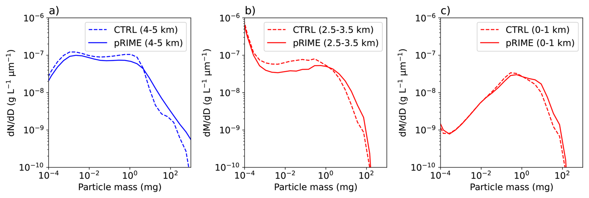
Figure B1 Averaged mass distributions at 2.5 h (TWC > 0.01 g m⁻³): ice mass distribution above the melting layer (4–5 km) in (a), drop mass distribution below the melting layer (2.5–3.5 km) in (b) and drop mass distribution averaged near the ground (0–1 km) in (c).