Paleoclimate data assimilation with adaptive observation error inflation and adaptive localization

Paleoclimate data assimilation methods significantly enhance the accuracy, spatiotemporal continuity, and global relevance of climate reconstructions by integrating Earth system models with proxy records. In this study, we further improve the algorithm by implementing two adaptive strategies – adaptive observation error inflation and adaptive localization – and systematically evaluate their performance in reconstructing temperature data over equatorial regions. For the adaptive observation error inflation experiments, two distinct methods were employed: the adaptive observation error inflation (AOEI) method yields significant improvements in specific regions but also introduces local biases, whereas the Huber Robust Estimation (HAOEI) method provides more robust and spatially consistent enhancements overall. In the adaptive localization experiments, the localization radius and weight matrix at each grid point are dynamically adjusted based on observational density and correlation information. This strategy effectively utilizes sparse observational data, suppresses spurious teleconnections, accurately reproduces the spatial structure of dominant climate variability modes, and thereby enhances the overall stability of the analyzed field.

1 Introduction

Reconstructing paleoclimate states is a crucial link in understanding the mechanisms and impacts of Earth system evolution. Currently, this field primarily relies on two methods: paleoclimate proxy records and Earth system model simulations. However, both approaches have significant limitations when reconstructing past climate states. On one hand, proxy records (such as tree rings, ice cores, speleothems, corals and etc.) play an indispensable role in reconstructing climate over the past millennia due to their long temporal span, but they often suffer from issues such as uneven spatiotemporal distribution, discontinuity, and sparsity. Furthermore, climate signals are easily contaminated by noise during preservation, making it extremely challenging to establish quantitative relationships between proxy indicators and the true climate state (Mann et al., 1998, 2008; Tingley et al., 2012; Liu et al., 2014; Guillot et al., 2015; Wang et al., 2015), and reconstructions of the same climate state from different proxy sources often show inconsistencies. On the other hand, climate models based on physical processes can provide physically consistent, globally complete climate fields with full spatiotemporal coverage, effectively capturing large-scale features of the climate system, however, due to inaccuracies in parameterizing physical processes and uncertainties in response to external forcings, model simulations may exhibit systematic biases, struggling to fully reproduce observed climate variability and leading to limited predictive skills (Widmann et al., 2010; Phipps et al., 2013; Kageyama et al., 2021). Therefore, to overcome the limitations of individual methods, paleoclimate data assimilation (PDA) techniques have emerged as a powerful tool to optimally merge information from proxy records – sparse, noisy, and indirect indicators of past climate – with the dynamical constraints of climate models (Von Storch et al., 2000; Hakim et al., 2016; Goosse, 2017). By doing so, the PDA method produces spatially complete and physically consistent climate field estimates, akin to reanalysis products for the instrumental era, while also quantifying reconstruction uncertainties. Among other methods, the Ensemble Kalman Filter (EnKF, Evensen, 1994), has gained prominence in PDA due to its easy implementation and capability to handle high-dimensional nonlinear systems (Hakim et al., 2016; Tardif et al., 2019; Osman et al., 2021; Sun et al., 2025). However, EnKF also suffers from sampling errors due to finite ensemble size, assumes near-Gaussian error distributions, and requires covariance localization to suppress spurious long-range correlations – issues that are particularly acute in paleoclimate applications with sparse proxies.

Despite the great potential of PDA, it faces unique challenges distinct from modern meteorological data assimilation, primarily due to the fact that proxy records are fairly sparse in time and space, and often represent time-averaged climatic signals (e.g., annual means) rather than instantaneous observations. Furthermore, proxy data are subject to complex errors arising from measurement inaccuracies, chronological uncertainties, and the imperfect relationship between proxy signals and the target climate variables. In the PDA, observation error variance is often specified empirically from the residual variance of a Proxy System Model (PSM, Evans et al., 2013; Dee et al., 2015; Zhu et al., 2023) calibrated against instrumental data. However, this method typically underestimates true proxy uncertainty, as it fails to account for calibration error (such as non-stationarity between past and instrumental periodes), structural error (arising from missing physics, biology, or chemistry in the PSM), and representation error (due to the mismatch between point-scale proxies and gridded state variables). To compensate, observation error inflation is frequently used (Sun et al., 2025). Given the strong spatial and temporal heterogeneity of proxy errors and information content, in PDA adaptive inflation methods are generally favored over a fixed inflation approach. While modern data assimilation has adopted techniques like Adaptive Observation Error Inflation (AOEI, Minamide and Zhang, 2017), its applicability to the specific challenges of the PDA remains insufficiently discussed and requires further exploration.

A critical factor for the success of the EnKF is its use of covariance localization. Early implementations typically employed a fixed localization radius (Houtekamer and Mitchell, 1998, 2001). Within this framework, a common approach is to taper the sampled covariances – between observations and model states, or between different model states – using a smooth, distance-dependent function. A standard choice for this function is the Gaussian-like Gaspari-Cohn (GC) function (Gaspari and Cohn, 1999). However, the Gaussian-like tapering function is not necessarily optimal as shown in several studies (Anderson, 2007; Lei and Anderson, 2014a, b). To address limitations of the fixed localization, a range of adaptive localization methods have been developed. Those methods adjust the localization often in response to the state-dependent correlation patterns or ensemble-estimated errors. Examples include techniques developed by Anderson (2007, 2012), Bishop and Hodyss (2009a, b), and Ménétrier et al. (2015a, b). However, these methods have yet to be applied to PDA context. In PDA, a large covariance localization radius is typically employed due to the sparse distribution of proxy records (Tardif et al., 2019). While necessary, an excessively large localization radius can introduce spurious long-distance correlations, ultimately degrading analysis quality. This limitation suggests that localization with a fixed radius is suboptimal for PDA applications. Instead, an adaptive localization, which can optimize the influence radius of observations based on the underlying spatial correlation structures, applying broader scales in regions with strong large-scale covariability and tighter constraints in data-rich or locally forced regions, is preferred. Currently, research on adaptive localization techniques in the PDA is still very limited.

In this paper, adaptive observation error inflation and adaptive covariance localization will be developed and explored within an ensemble-based PDA framework, aiming to create a more flexible and accurate assimilation system. As a methodological paper, a pseudoproxy experiment might be more informative than a real-word one. But we directly conduct real-world proxy experiments using a climate model to systematically evaluate whether these adaptive strategies can enhance reconstruction skill – particularly in sparse data regimes – improve uncertainty quantification, and provide a more generalizable approach for assimilating the heterogeneous and uncertain proxy records that characterize paleoclimatology.

2 Methods

2.1 Offline Data Assimilation

The offline EnKF is a widely used approach for paleoclimate data assimilation, popularized in the paleoclimate context by Steiger et al. (2014), Hakim et al. (2016), and Tardif et al. (2019). “Offline” means that the background ensemble is static – typically drawn from climate model simulations covering the entire reconstruction period – rather than evolving through a continuous forecast cycle. The state update equation is given by

$$\begin{array}{}\text{(1)}& {\mathit{x}}_a={\mathit{x}}_b+\mathbf{K}\left[\mathit{y}-{\mathit{y}}_e\right],\end{array}$$

where x_b is the ensemble prior. The vector y represents the assimilated proxy data, and y_e = H(x_b) is the vector of proxy estimates derived from the prior through the forward operator H. K is the Kalman gain matrix:

$$\begin{array}{}\text{(2)}& \mathbf{K}={\mathbf{BH}}^T{\left[{\mathbf{HBH}}^T+\mathbf{R}\right]}^{-\mathrm{1}},\end{array}$$

where B is the prior covariance matrix, R is the error covariance matrix of the proxy data, and H is the linearization of the forward operator H about the prior mean. The above Eq. (1) is solved using the ensemble square-root filter (EnSRF, Whitaker and Hamill, 2002). R is taken as a diagonal matrix (uncorrelated observation errors), with the diagonal elements representing the error variance for each assimilated proxy record (Tardif et al., 2019). This allows for serial processing of observations, in which observations are assimilated one at a time, greatly simplifying the implementation of covariance localization. For a single jth proxy data y_j, the ensemble mean is updated by

$$\begin{array}{}\text{(3)}& {\stackrel{\mathrm{‾}}{\mathit{x}}}_a={\stackrel{\mathrm{‾}}{\mathit{x}}}_b+{\displaystyle \frac{w_{\mathrm{loc}}\circ \text{cov}\left({\mathit{x}}_b,{\mathit{y}}_{\mathrm{e},j}\right)}{\text{var}\left({\mathit{y}}_{\mathrm{e},j}\right)+R_j}}\left({\mathit{y}}_j-{\stackrel{\mathrm{‾}}{\mathit{y}}}_{\mathrm{e},j}\right),\end{array}$$

where ${\stackrel{\mathrm{‾}}{\mathit{y}}}_{\mathrm{e},j}={\stackrel{\mathrm{‾}}{H\left({\mathit{x}}_b\right)}}_j$ is the prior estimate of the jth proxy from the ensemble mean, R_j is the observation error variance for the jth proxy record, and cov() and var() denote the covariance and variance functions. Covariance localization is represented by the Schur product (denoted by ∘, i.e., element-wise multiplication) in the equation, which acts as a distance-weighted filter w_loc on the prior covariance matrix to suppress spurious long-distance correlations. The jth ensemble perturbation is updated by

$$\begin{array}{}\text{(4)}& {\mathit{x}}_a^{\prime }={\mathit{x}}_b^{\prime }-{\left[\mathrm{1}+\sqrt{{\displaystyle \frac{R_j}{\text{var}\left({\mathit{y}}_{\mathrm{e},j}\right)+R_j}}}\right]}^{-\mathrm{1}}{\displaystyle \frac{w_{\mathrm{loc}}\circ \text{cov}\left({\mathit{x}}_b,{\mathit{y}}_{\mathrm{e},j}\right)}{\text{var}\left({\mathit{y}}_{\mathrm{e},j}\right)+R_j}}\left({\mathit{y}}_{\mathrm{e},j}^{\prime }\right).\end{array}$$

2.2 Adaptive observation error inflation

The AOEI was first introduced and systematically applied in the context of satellite radiance data assimilation for numerical weather prediction (Minamide and Zhang, 2017). For the jth proxy, it operates as in Eq. (5) by inflating the observation error variance when the squared innovation – the difference between the observation and the model simulation – exceeds the ensemble spread of the model simulation:

$$\begin{array}{}\text{(5)}& R_j=max\left\{{\mathit{\sigma }}_{\mathrm{o},j}^{\mathrm{2}},{\left[{\mathit{y}}_j-{\stackrel{\mathrm{‾}}{\mathit{y}}}_{\mathrm{e},j}\right]}^{\mathrm{2}}-{\mathit{\sigma }}_{{\mathit{y}}_e,j}^{\mathrm{2}}\right\},\end{array}$$

where ${\mathit{\sigma }}_{\mathrm{o},j}^{\mathrm{2}}$ is original observation error variance, y_j is the jth proxy value, ${\stackrel{\mathrm{‾}}{\mathit{y}}}_{\mathrm{e},j}={\stackrel{\mathrm{‾}}{H\left({\mathit{x}}_b\right)}}_j$ is the prior estimate of the jth proxy from the ensemble mean, H is the observation forward operator, $[{\mathit{y}}_j-{\mathit{y}}_{\mathrm{e},j}]$ is the innovation, and ${\mathit{\sigma }}_{{\mathit{y}}_{\mathrm{e},j}}^{\mathrm{2}}$ is the ensemble spread in observation space.

The AOEI is designed to limit erroneous analysis increments where there are large representativeness errors in either the forecast model and/or from the observation itself. However, its aggressive adjustment strategy (inflation grows with the square of innovation) requires careful application in data-sparse regions or areas with uncertain observations to avoid amplifying noise.

2.3 Huber Robust Estimation

In this study, a new adaptive observation error inflation scheme based on the Huber robust estimation method (Huber, 1992) is introduced (hereafter called “HAOEI”), which aims to mitigate the undue influence of large outliers. This method computes a normalized innovation – the difference between the observation and the model forecast, normalized by the square root of the sum of the model forecast error variance and the baseline observational error variance – and compares it against a threshold δ. The baseline observational error variance is then inflated for values exceeding this threshold. For the jth proxy, the simplified formulation is as follows:

$$\begin{array}{}\text{(6)}& {\displaystyle }{r}_j={\displaystyle \frac{{\mathit{y}}_j-{\stackrel{\mathrm{‾}}{\mathit{y}}}_{\mathrm{e},j}}{\sqrt{{\mathit{\sigma }}_{\mathrm{o},j}^{\mathrm{2}}+{\mathit{\sigma }}_{{\mathit{y}}_{\mathrm{e},j}^{\mathrm{2}}}}}},\text{(7)}& {\displaystyle }{R}_j=\left\{\begin{array}{ll}{\mathit{\sigma }}_{\mathrm{o},j}^{\mathrm{2}},& \text{for}\left|r_j\right|\le \mathit{\delta },\\ {\mathit{\sigma }}_{\mathrm{o},j}^{\mathrm{2}}\cdot \frac{\left|r_j\right|}{\mathit{\delta }},& \text{for}\left|r_j\right|>\mathit{\delta }.\end{array}\right.\end{array}$$

where ${\mathit{\sigma }}_{\mathrm{o},j}^{\mathrm{2}}$ is the uninflated observation error variance, y_j is the jth proxy value, ${\stackrel{\mathrm{‾}}{\mathit{y}}}_{\mathrm{e},j}={\stackrel{\mathrm{‾}}{H\left({\mathit{x}}_b\right)}}_j$ is the model estimated proxy using the ensemble mean of climatological samples, H is the observation forward operator and ${\mathit{\sigma }}_{{\mathit{y}}_e,j}^{\mathrm{2}}$ is the ensemble spread in observation space. The threshold parameter δ defines the boundary between normal observations and potential outliers, typically chosen based on statistical significance levels (e.g., δ ≈ 1.645 corresponds to the 90 % confidence interval of a standard normal distribution). Observations with normalized innovations within ±δ are considered statistically consistent with the forecast and retain their original error variance, while those beyond this range are treated as potential outliers and undergo error variance inflation.

Although δ introduces an additional degree of freedom, δ can be chosen based on statistical significance levels. For example, δ ≈ 1.645 corresponds to the 90 % confidence interval of a standard normal distribution. This provides a theoretically grounded starting point, rather than purely empirical tuning. In practice, δ can be selected using cross-validation or calibrated against reference periods (e.g., the instrumental era) when available. Compared to AOEI that inflates the observation error variance quadratically with the innovation, which can over-penalize observations in regions with poor model priors and thus lead to local degradation, HAOEI addresses this by first normalizing the innovation by the combined forecast and observation uncertainty. Only when this normalized residual exceeds a predefined threshold δ (e.g., corresponding to a 90 % confidence interval) does it inflate the error variance, and the inflation is linear rather than quadratic. This follows the logic of Huber's estimationr: observations within the expected range are trusted, while those outside are down-weighted gradually, not abruptly or excessively. Therefore, the HAOEI applies a more moderate, linear inflation only after a threshold is crossed. This design makes it a robust stabilizer: it consistently improves performance across wider areas by avoiding extreme adjustments, even if it does not achieve the same peak correction in the most mismatched locations.

2.4 Adaptive localization

Due to the uneven spatial distribution of proxy data, localization is required to constrain their spurious influence on remote regions. Within a fixed localization radius PDA framework, a weight matrix was introduced by Tardif et al. (2019) to adjust the covariance. This weight matrix is defined by the Gaspari-Cohn function (Gaspari and Cohn, 1999):

$$\begin{array}{}\text{(8)}& w_{ij}=\text{GC}(d_{ij},L)\end{array}$$

where w_ij is the weight assigned to observation y_j when updating grid point x_i, d_ij is the distance between grid point and observation, L is a specified cut-off (or localization) radius, and GC denotes the Gaspari-Cohn fifth-order polynomial:

$$\begin{array}{}\text{(9)}& \begin{array}{rl}& \text{GC}\left(z_{ij}\right)=\\ & \left\{\begin{array}{ll}\mathrm{1}-\frac{\mathrm{5}}{\mathrm{3}}{z}_{ij}^{\mathrm{2}}+\frac{\mathrm{5}}{\mathrm{8}}{z}_{ij}^{\mathrm{3}}+\frac{\mathrm{1}}{\mathrm{2}}{z}_{ij}^{\mathrm{4}}-\frac{\mathrm{1}}{\mathrm{4}}{z}_{ij}^{\mathrm{5}},& \mathrm{0}\le z_{ij}\le \mathrm{1}\\ -{\displaystyle \frac{\mathrm{2}}{\mathrm{3}}}{z}_{ij}^{-\mathrm{1}}+\mathrm{4}-\mathrm{5}{z}_{ij}+{\displaystyle \frac{\mathrm{5}}{\mathrm{3}}}{z}_{ij}^{\mathrm{2}}+{\displaystyle \frac{\mathrm{5}}{\mathrm{8}}}{z}_{ij}^{\mathrm{3}}-{\displaystyle \frac{\mathrm{1}}{\mathrm{2}}}{z}_{ij}^{\mathrm{4}}+{\displaystyle \frac{\mathrm{1}}{\mathrm{12}}}{z}_{ij}^{\mathrm{5}},& \mathrm{1}<z_{ij}\le \mathrm{2}\\ \mathrm{0},& z_{ij}>\mathrm{2}\end{array}\right.\end{array}\end{array}$$

where z_ij = $\frac{d_{ij}}{L/\mathrm{2}}$.

This method uses a fixed localization radius with the GC function, which tapers covariances based solely on physical distance. However, this method has two major limitations when applied to PDA: (1) Fixed radius ignores varying data density: In data-dense regions, a large fixed radius unnecessarily smooths fine-scale variability and introduces spurious correlations. In data-sparse regions, a small radius would discard too much information, while a large radius risks including irrelevant remote proxies. An adaptive radius that responds to local observational density can better balance these competing needs. (2) Distance alone misses teleconnections: Important climate phenomena such as ENSO involve strong correlations over large distances. A purely distance-based cutoff (like GC) may either exclude these physically meaningful teleconnections (if the radius is too small) or include many spurious ones (if the radius is too large). Thus, a two-component adaptive strategy is proposed: (1) a density-dependent localization radius to handle heterogeneous data coverage. (2) Correlation-based weighting to identify and preserve genuine teleconnections beyond the distance cutoff.

Observational density is estimated at each grid point using kernel density estimation (KDE) with a Gaussian kernel (Parzen, 1962). For a given grid point x_i, the density is computed as:

$$\begin{array}{}\text{(10)}& {\mathit{\rho }}^{*}\left({\mathit{x}}_i\right)={\displaystyle \frac{\mathrm{1}}{n{h}^{\mathrm{2}}}}\sum _{j=\mathrm{1}}^{n}K\left({\displaystyle \frac{\Vert {\mathbf{o}}_i-{\mathbf{o}}_j\Vert }{h}}\right)\end{array}$$

where n is the total number of proxy observations, o_i denotes the location of the grid point x_i, o_j denotes the location of the jth observation, $\Vert \cdot \Vert$ denotes the euclidean distance between two points, h is the bandwidth parameter, and K(⋅) is the Gaussian kernel function:

$$\begin{array}{}\text{(11)}& K\left(u\right)={\displaystyle \frac{\mathrm{1}}{\mathrm{2}\mathit{\pi }}}{e}^{-\frac{u^{\mathrm{2}}}{\mathrm{2}}}.\end{array}$$

The bandwidth h is determined using Scott's rule:

$$\begin{array}{}\text{(12)}& h=n^{-\mathrm{1}/\mathrm{6}}\cdot \widehat{\mathit{\sigma }},\end{array}$$

where $\widehat{\mathit{\sigma }}$ is the standard deviation of the observation locations (computed from their longitudes and latitudes). This choice provides a data-adaptive smoothing that balances bias and variance in density estimation, yielding a continuous density field. This density field is then normalized by its global maximum value to obtain $\mathit{\rho }\left({\mathit{x}}_i\right)\in [\mathrm{0},\mathrm{1}]$, representing the relative data density at grid point x_i. Based on this, the localization radius L(x_i) at grid point x_i is defined as a function of this normalized density.

$$\begin{array}{}\text{(13)}& \begin{array}{rl}& L\left({\mathit{x}}_i\right)\\ & =\left\{\begin{array}{ll}L\cdot (\mathrm{1}-\mathit{\rho }({\mathit{x}}_i{)}^{\mathrm{1}/\mathrm{2}}),& \text{if}L\cdot (\mathrm{1}-\mathit{\rho }({\mathit{x}}_i{)}^{\mathrm{1}/\mathrm{2}})\ge L_{min}\\ L_{min},& \text{otherwise}\end{array}\right.\end{array}\end{array}$$

where L is the original fixed localization radius (attained in observation-sparse regions where ρ(x_i) → 0), the exponent $\mathrm{1}/\mathrm{2}$ controls the curvature of the density-to-radius mapping, and L_min is a lower bound enforced to maintain a minimum influence range even in observation-dense regions.

However, adjusting the localization radius solely based on density may further reduce the number of effective observations available for some grid points. While this helps suppress spurious teleconnections, it can also limit the use of already sparse paleoclimate proxy data, potentially undermining assimilation performance.

To better balance the use of observational information and the suppression of spurious correlations, we further incorporate correlation information into the weighting strategy, i.e., for observations outside the localization radius, their influence weight depends on the correlation (w_ij ∼ corr). The correlation coefficient r_ij between grid point x_i and observation y_j is computed as the Pearson correlation coefficient between their respective time series over the reconstruction period:

$$\begin{array}{}\text{(14)}& r_{ij}={\displaystyle \frac{{\sum }_{t=\mathrm{1}}^T\left({\mathit{x}}_{i,t}-{\stackrel{\mathrm{‾}}{\mathit{x}}}_i\right)\left({\mathit{y}}_{j,t}-{\stackrel{\mathrm{‾}}{\mathit{y}}}_j\right)}{\sqrt{{\sum }_{t=\mathrm{1}}^T{\left({\mathit{x}}_{i,t}-{\stackrel{\mathrm{‾}}{\mathit{x}}}_i\right)}^{\mathrm{2}}{\sum }_{t=\mathrm{1}}^T{\left({\mathit{y}}_{j,t}-{\stackrel{\mathrm{‾}}{\mathit{y}}}_j\right)}^{\mathrm{2}}}}},\end{array}$$

where x_i,t is the value at grid point x_i at time t, y_j,t is the value at observation x_j at time t, ${\stackrel{\mathrm{‾}}{\mathit{x}}}_i$ and ${\stackrel{\mathrm{‾}}{\mathit{y}}}_j$ are the temporal means of the respective series, and T is the length of the time series. This coefficient quantifies the statistical relationship between distant locations and helps identify teleconnections that are physically meaningful rather than spurious.

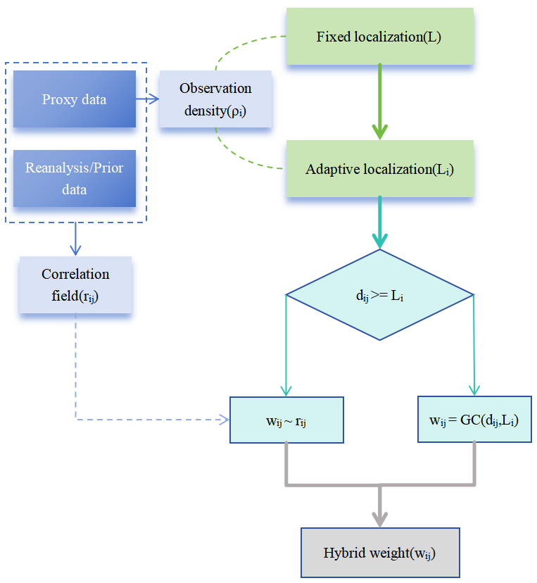
The final weight w_ij assigned to observation x_j when updating grid point x_i is then defined as a hybrid of distance-based and correlation-based weighting:

$$\begin{array}{}\text{(15)}& w_{ij}=\left\{\begin{array}{ll}\frac{\mathrm{1}}{\mathrm{2}}\cdot \left|r_{ij}\right|,& \text{if}{d}_{ij}>L_i\text{and}\left|r_{ij}\right|>\mathrm{0.2}\\ \text{GC}(d_{ij},L_i),& \text{else}\end{array}\right.\end{array}$$

where d_ij is the distance between grid point x_i and observation y_j, L_i = L(x_i) is the adaptive localization radius at grid point x_i computed from Eq. (13), r_ij is the correlation coefficient, 0.2 is the set expression threshold.

Figure 1 illustrates the flowchart of this method. Compared to the standard fixed-radius GC function, the new method is superior because it is spatially adaptive and information-aware. The GC applies the same tapering everywhere regardless of how many proxies are available, which is suboptimal for heterogeneous networks. The KDE-based radius shrinks in data-rich areas to preserve local details and expands in data-poor areas to gather more information. The correlation-based component further adds value by recovering remote signals that GC would completely zero out. Compared to other existing adaptive localization methods (e.g., Anderson, 2012; Bishop and Hodyss, 2009a, b; Ménétrier et al., 2015a, b), this approach is specifically tailored to the challenges of the PDA. Many of those methods were developed for dense observing networks (e.g., satellite radiances or radiosondes). The new method preserves the stability of distance-based localization within the adaptive radius while selectively adding distant, highly correlated observations – a feature not present in most existing adaptive schemes. It is specifically designed for sparse, unevenly distributed proxy networks and directly addresses the two key weaknesses of fixed-radius GC (ignoring data density and teleconnections).

Figure 1 Flowchart of the adaptive localization method.

Finally, it is worth noting that h is a parameter in the mathematical sense, which is determined uniquely from the data and does not introduce additional user-specific uncertainty. L_min is physically meaningful and easy to set. The minimum localization radius L_min is introduced to prevent the radius from becoming zero in very data-dense regions. Even in the densest proxy network, a zero radius would discard all observations, which is clearly undesirable. L_min does not rely on an exquisitely precise value but it should be set to a reasonably small value that can be guided by the typical decorrelation length scale of the climate variables.

3 Experimental design and results

3.1 Experimental design

To evaluate the effectiveness of adaptive inflation and adaptive localization methods, a set of sensitivity experiments (Table 1) is conducted using the cfr framework (v2024.1.26; Zhu et al., 2024b), which is a Python-based package that provides a suite of ensemble-based data assimilation and reconstruction tools, including EnKF implementation, proxy system models, and verification diagnostics. It is specifically designed for paleoclimate applications and is openly available. The goal is to reconstruct tropical (30° S–30° N) surface temperature anomalies from 1880 to 2000, with respect to the 1951–1980 climatological baseline. The prior ensemble is drawn from the “iCESM1” last millennium and historical simulations (Brady et al., 2019), which provide physically consistent climate backgrounds spanning 850–2000 CE. Coral-based proxy records from the PAGES 2k Phase 2 database (PAGES 2k Consortium, 2017) – calibrated against NASA GISTEMP v4 (Lenssen et al., 2019) – are assimilated. These records are selected due to their strong temperature sensitivity and predominant distribution within the tropics (Fig. 2). Focusing on the tropics is motivated by two main reasons: first, the high temperature sensitivity of coral proxies enhances reconstruction reliability, whereas incorporating other proxy types (e.g., tree rings, ice cores) at a global scale could increase uncertainty due to their generally lower temperature sensitivity. Second, the tropics contain key climate systems such as ENSO, frequently studied in paleoclimatology, allowing for a clear assessment of methodological performance while reducing computational costs. It is important to note that the methodology presented here can, in principle, be extended to global applications. In the following, the impact of adaptive observation error is first assessed by comparing two inflation schemes – AOEI and HAOEI. Next, sensitivity experiments investigate the role of localization. Initial tests use fixed localization radii, which are then compared to two experiments employing the adaptive localization method described in Sect. 2.4 – one estimating proxy-state correlations based on reanalysis data GISTEMP v4, and the other one based on the model priors from “ICESM1” last millennium simulations. All data assimilation experiments cover 1880–2000, use a 1-year assimilation window, and an ensemble size of 100.

Table 1 Experimental setups, which are divided into two groups, sensitivity experiments on observation error inflation and on localization.

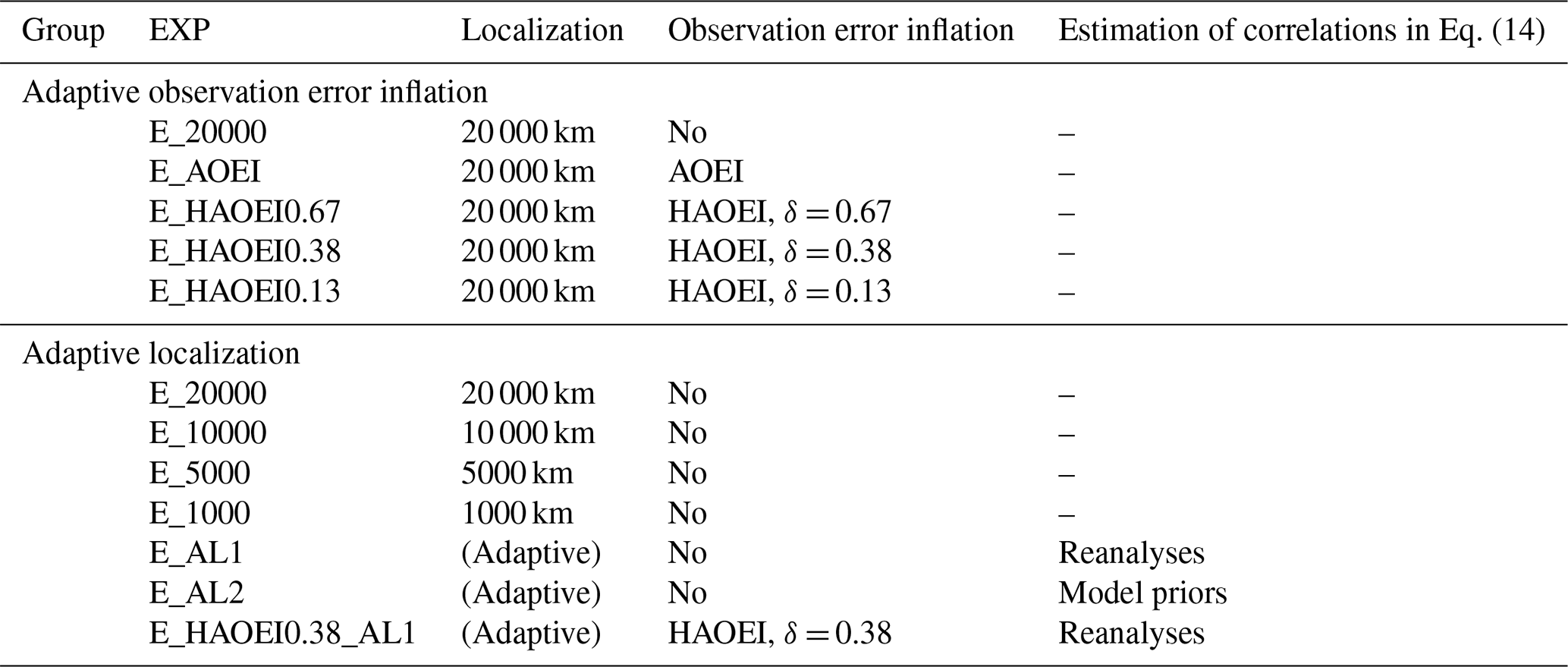
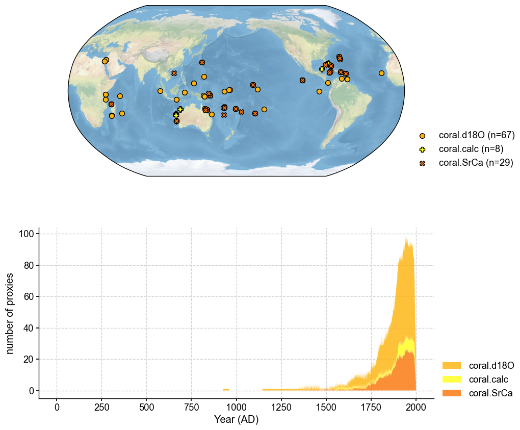
Figure 2 Spatial and temporal distributions of proxy records from the PAGES 2k dataset, visualized with cfr (Zhu et al., 2024b).

Three metrics are computed to evaluate the reconstruction analyses: the Root Mean Square Error (RMSE), the Coefficient of Efficiency (CE), and the Empirical Orthogonal Function (EOF). The RMSE for a given model grid point q is defined as:

$$\begin{array}{}\text{(16)}& \text{RMSE}\left(q\right)=\sqrt{{\displaystyle \frac{\mathrm{1}}{n}}\sum _{t=\mathrm{1}}^n{\left({\mathbf{v}}_{q,t}-{\stackrel{\mathrm{‾}}{\mathbf{x}}}_{q,t}\right)}^{\mathrm{2}}},\end{array}$$

where n is the number of time samples, v_q,t is the verification data at grid point q and time t, and ${\stackrel{\mathrm{‾}}{\mathbf{x}}}_{q,t}$ is the corresponding prior or posterior ensemble mean.

The CE evaluates the skill of the reconstruction relative to the climatological mean of the verification data. For a given model grid point q, it is calculated as:

$$\begin{array}{}\text{(17)}& \text{CE}\left(q\right)=\mathrm{1}-{\displaystyle \frac{{\sum }_{t=\mathrm{1}}^n{\left({\mathbf{v}}_{q,t}-{\stackrel{\mathrm{‾}}{\mathbf{x}}}_{q,t}\right)}^{\mathrm{2}}}{{\sum }_{t=\mathrm{1}}^n{\left({\mathbf{v}}_{q,t}-{\stackrel{\mathrm{‾}}{\mathbf{v}}}_q\right)}^{\mathrm{2}}}},\end{array}$$

where ${\stackrel{\mathrm{‾}}{\mathbf{v}}}_q$ is the temporal mean of the verification data at grid point q. A CE value close to 1.0 indicates a highly accurate reconstruction, a value of 0 means the reconstruction is only as accurate as the climatological mean, and negative values suggest lower skill.

Beyond pointwise accuracy metrics, we also examine the ability of the reconstructions to capture the dominant large-scale modes of climate variability. For this purpose, we apply Empirical Orthogonal Function (EOF) analysis (Lorenz, 1956) to the reconstructed spatial fields The EOF method decomposes a spatiotemporal field X(s,t) into a set of orthogonal spatial patterns (EOFs) and their associated principal component (PC) time series. The leading EOF mode explains the largest possible fraction of the total variance, with each subsequent mode explaining the maximum remaining variance under the constraint of orthogonality to all previous modes. The corresponding PC represent the temporal evolution of these spatial patterns. In the following analysis, we compare the leading EOF modes – their spatial patterns, explained variance – obtained from different reconstruction methods against those derived from the verification dataset, to assess which method better recovers the key climate teleconnections and oscillatory signals.

As validation data, the spatially completed version of the near-surface air temperature and sea-surface temperature analyses product HadCRUT4.6 (Vaccaro et al., 2021) is employed.

3.2 Results

3.2.1 Adaptive observation error inflation

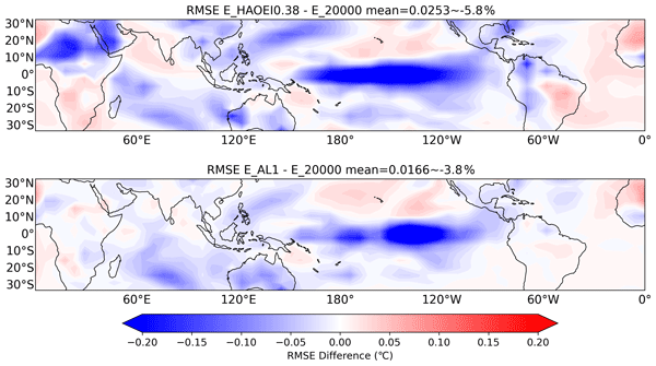
Figure 3 shows the RMSE for the surface temperature analyses in experiment E_20000, as well as the RMSE and percentage RMSE differences between E_20000 and E_AOEI, E_HAOEI(0.67), E_HAOEI(0.38), and E_HAOEI(0.13). The largest RMSE values in E_20000 are located in the equatorial ENSO region. E_AOEI produces a noticeable reduction in RMSE relative to E_20000 (mean difference = −0.0195 °C, approximately 4.5 %). This improvement stems primarily from its aggressive error-inflation strategy, which strongly down-weights observations that deviate sharply from the model prior-most effectively in regions such as the ENSO zone where model biases are large. However, the same mechanism can also suppress accurate observations where the prior is poor, leading to local error increases, as seen over the North Pacific and Atlantic.The HAOEI method applies a more moderate, threshold-dependent inflation. E_HAOEI(0.67) yields widespread and modest improvements, with a mean RMSE difference of −0.0210 °C (a reduction of 4.8 %). E_HAOEI(0.38) delivers a stronger overall error reduction (mean difference = −0.0253 °C, a reduction of approximately 5.8 %) and outperforming both E_AOEI and E_HAOEI(0.67). However, E_HAOEI(0.13) still achieves some improvement (RMSE difference = −0.0208 °C, a reduction of 4.7 %), its performance is inferior to that of E_HAOEI(0.38). Similar performance patterns are reflected in the CE results (Fig. 4). While E_AOEI yields considerably higher CE values than E_20000 (0.1201 compared to −0.2106), tuning the δ parameter can adjust the skill, the mean CE values in E_HAOEI(0.67), E_HAOEI(0.38) and E_HAOEI(0.13) are 0.1275, 0.1514 and 0.1297, respectively, demonstrating a comprehensively better performance of E_HAOEI(0.38) overall. Hence, the choice of the threshold δ in HAOEI involves a fundamental trade-off: a value that is too small (e.g., 0.13) makes the method overly sensitive, flagging even moderate model-observation mismatches as outliers and down-weighting them, which leads to excessive loss of useful information and degraded analysis quality; conversely, a value that is too large (e.g., 0.67) makes the method overly conservative, affecting only the most extreme observations and failing to adequately control many genuinely large errors, thereby yielding only limited improvements. The optimal value (e.g., 0.38) strikes the best balance – maximizing the correction of harmful errors while minimizing the unnecessary loss of informative observations.

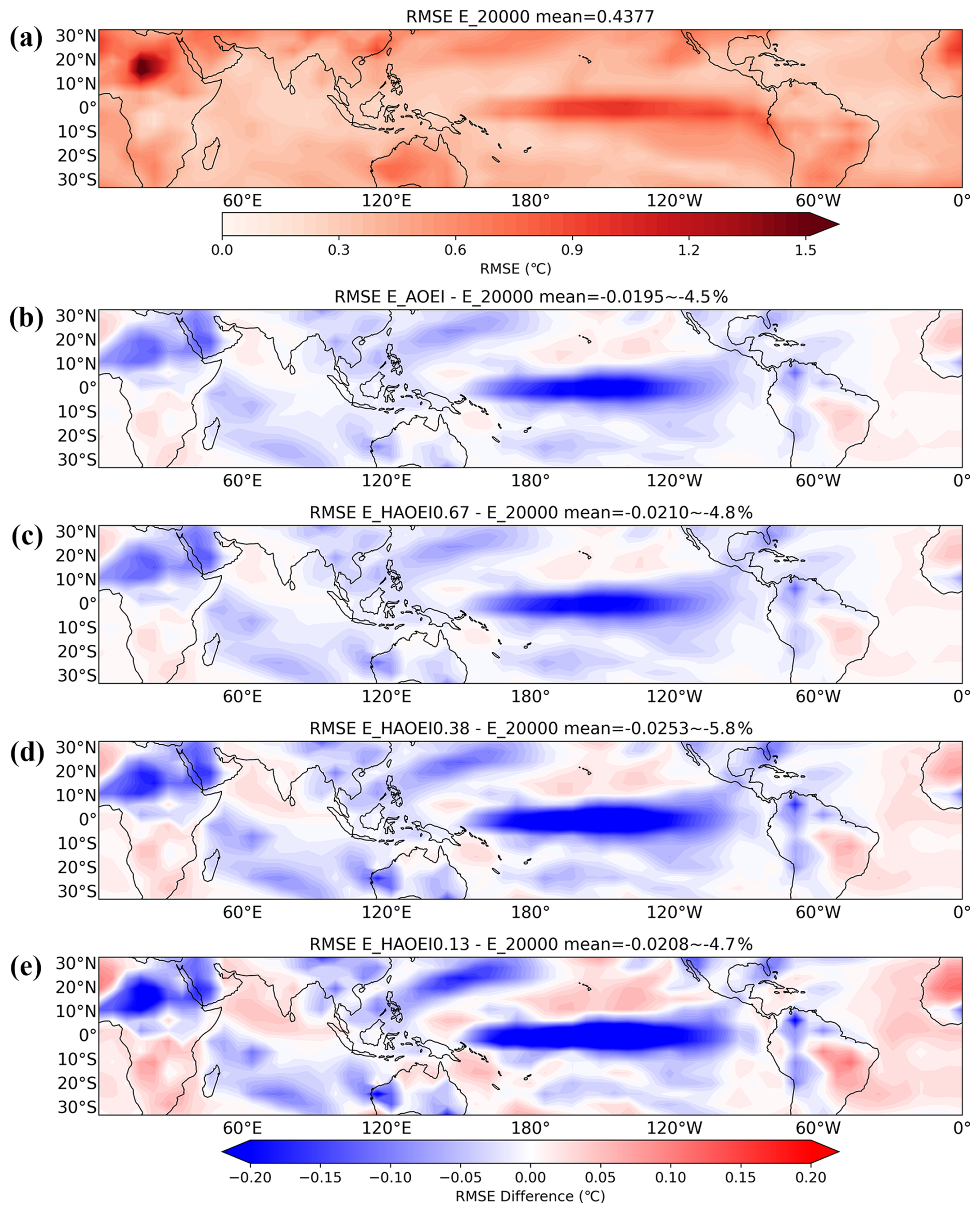
Figure 3 (a) The RMSE for the surface temperature analyses in E_20000, (b) the RMSE differences and the percentage RMSE differences between E_AOEI and E_20000, (c) between E_HAOEI0.67 and E_20000, (d) between E_HAOEI0.38 and E_20000, and (e) between E_HAOEI0.13 and E_20000.

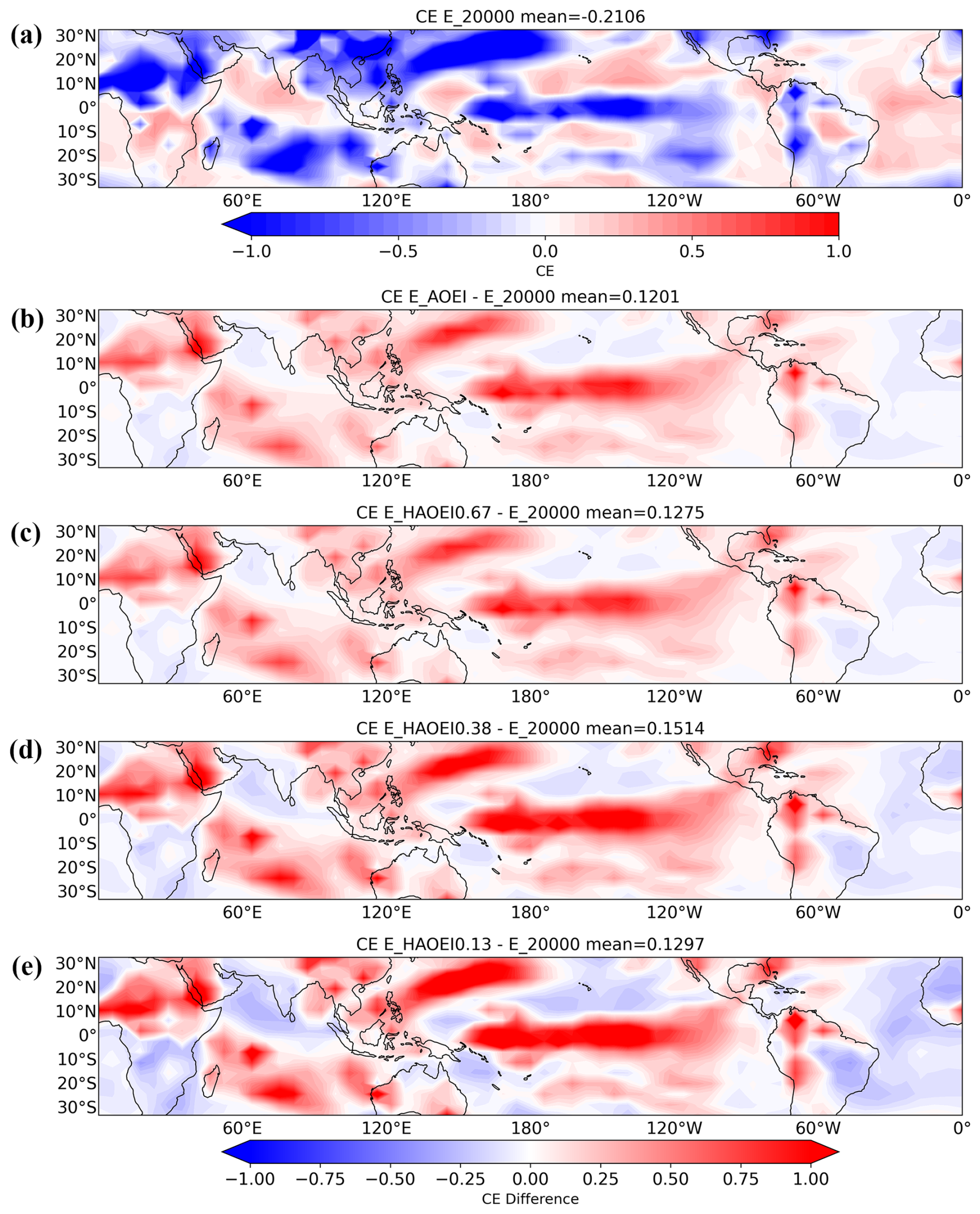
Figure 4 Same as Fig. 3 but for the CE.

Figure 5 compares the spatial pattern and PC time series of the leading EOF mode derived from the observations with those from the reconstructed analyses of E_AOEI, E_HAOEI(δ = 0.67), E_HAOEI(δ = 0.38) and E_HAOEI(δ = 0.13). All experiments display a similar spatial structure to the observations, yet they show markedly stronger variability in the ENSO region and produce a substantially higher explained variance. This discrepancy suggests that within the current assimilation framework, the reconstructed temperature field may be overly focused on a single dominant spatial mode, thereby failing to capture the more dispersed, multi-scale variability present in the actual observations. This effect may be partly due to the use of an excessively large localization radius, a point that will be further discussed in the following section.

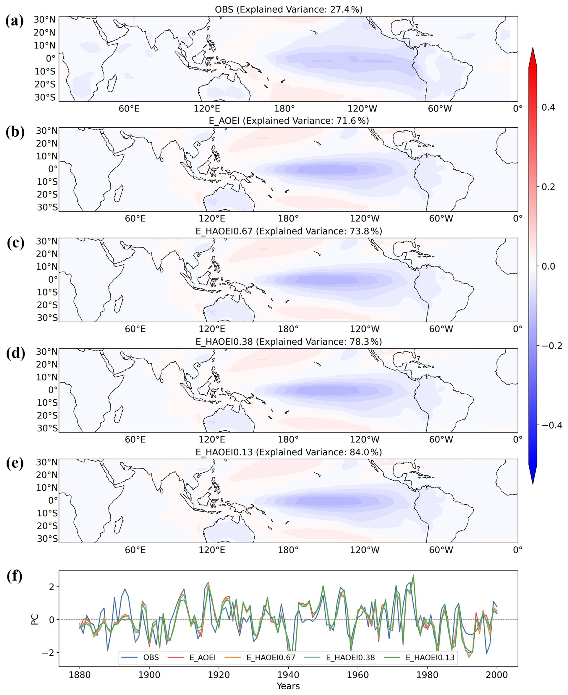
Figure 5 The leading EOF mode of (a) observations (b) E_AOEI analyses (c) E_HAOEI (δ=0.67) analyses (d) E_HAOEI (δ = 0.38) analyses (e) E_HAOEI (δ = 0.13) analyses (f) corresponding PC time series for all experiments.

3.2.2 Adaptive localization

Figure 6 presents the time series of RMSE for surface temperature analyses across experiments using different fixed localization radii (1000–20 000 km). As the localization radius grows, the RMSE decreases from 0.4377 in E_20000 to 0.4234 in E_5000, and increases again to 0.4307 in E_1000. This behavior is consistent with other studies (e.g., Zeng and Janjić, 2016). More importantly, regarding the leading EOF mode as shown in Fig. 7, smaller radii significantly distort the spatial pattern of variability, although they explained variance values closer to those of the observations (66.7 % in E_20000 and 27.3 % in E_1000 compared to 27.4 % in observations). This seemingly paradoxical behavior-where RMSE first decreases and then increases as the localization radius shrinks, while the EOF spatial pattern becomes progressively distorted-reflects the fundamental trade-off between sampling error and the retention of physically meaningful large-scale teleconnections in ensemble-based data assimilation. A large radius (e.g., 20 000 km) allows each grid point to be influenced by distant observations, preserving coherent large-scale structures (such as the ENSO pattern) and yielding a spatially reasonable EOF mode, but it also introduces spurious long-distance correlations from sampling noise, which inflates both the RMSE and the explained variance of the leading EOF. Reducing the radius to an intermediate value (e.g., 5000 km) effectively suppresses many of these spurious correlations, leading to a lower RMSE and a more physical analysis. However, when the radius becomes too small (e.g., 1000 km), the assimilation overly relies on local observations, cutting off genuine large-scale connections and fragmenting the spatial structure; although this yields a notably lower RMSE and an explained variance that matches the observations, the leading EOF mode becomes spatially distorted and physically unrealistic-demonstrating that numerical metrics like RMSE and variance explained are insufficient indicators of physical fidelity.

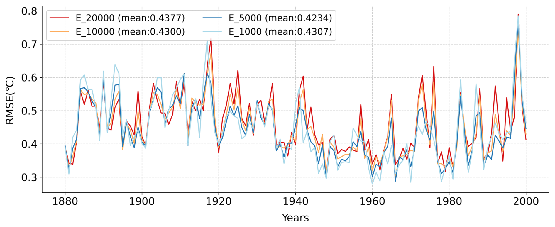
Figure 6 The time series of the RMSE for the surface temperature analyses in experiments with varying fixed localization radii.

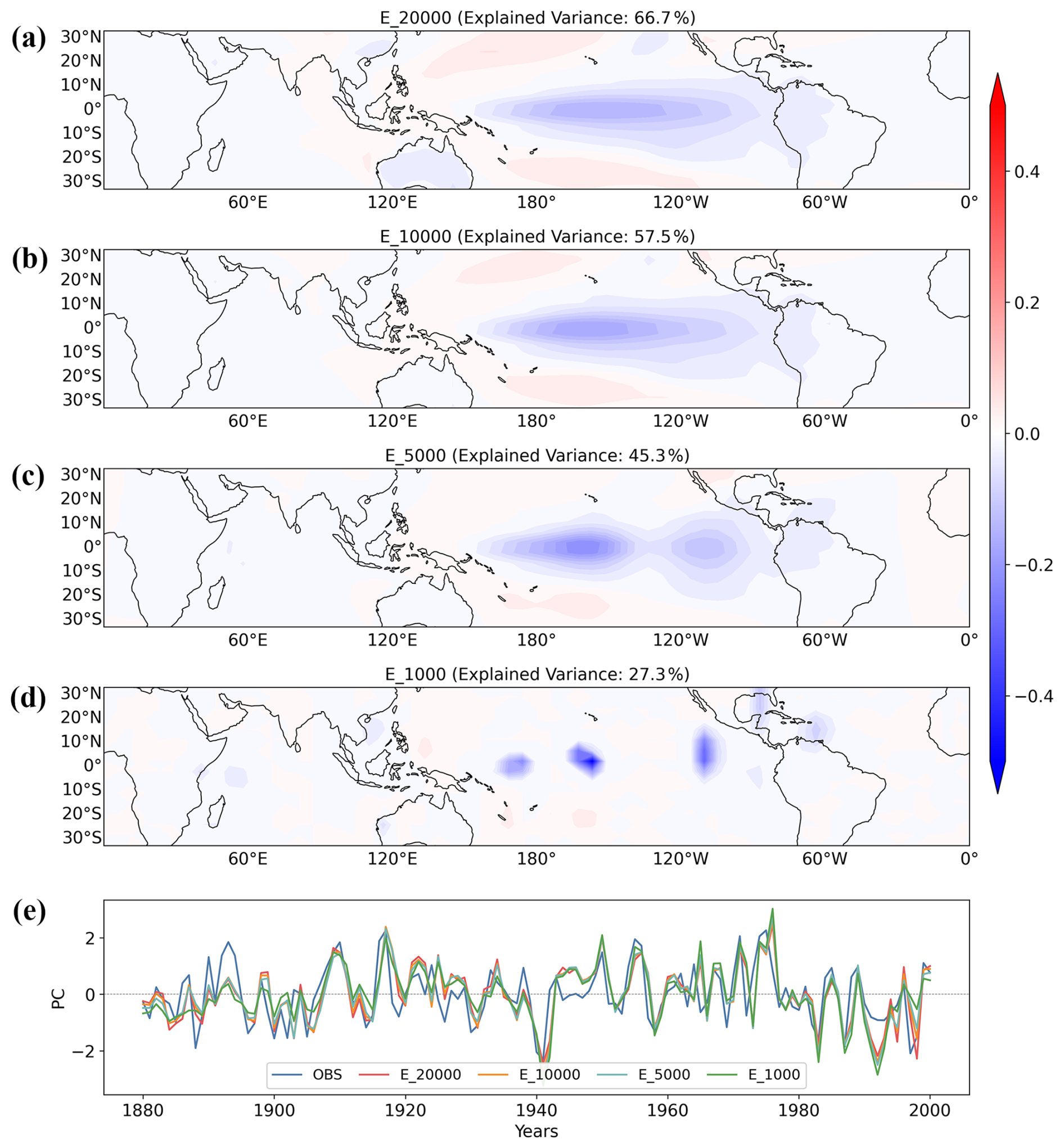
Figure 7 The leading EOF mode of the tropics: (a) reconstructed EOF field with 20 000 km localization radius; (b) reconstructed EOF field with 10 000 km localization radius; (c) reconstructed EOF field with 5000 km localization radius; (d) reconstructed EOF field with 1000 km localization radius; (e) corresponding PC time series for all experiments. All results are based on the period 1880–2000. EOF units are °C.

To implement the adaptive localization method described in Sect. 2.4, the spatial density of proxy records is first estimated using kernel density estimation (KDE), as visualized in Fig. 8. While this density varies from year to year, the time-averaged distribution reveals distinct regional patterns: Australia and Central America are data-rich, the equatorial ENSO region exhibits medium proxy density, and areas such as South America remain relatively data-sparse. Furthermore, proxy-state correlations given in Eq. (14) are given by using the reanalyses and model priors, respectively. Figure 9 illustrates the correlations for one representative proxy record (ID: Ocn_090). Both estimated correlations reflect similar spatial structures but with detailed differences, e.g., the former one shows generally higher values and distinct discrepancies over Africa and the adjacent Indian Ocean region.

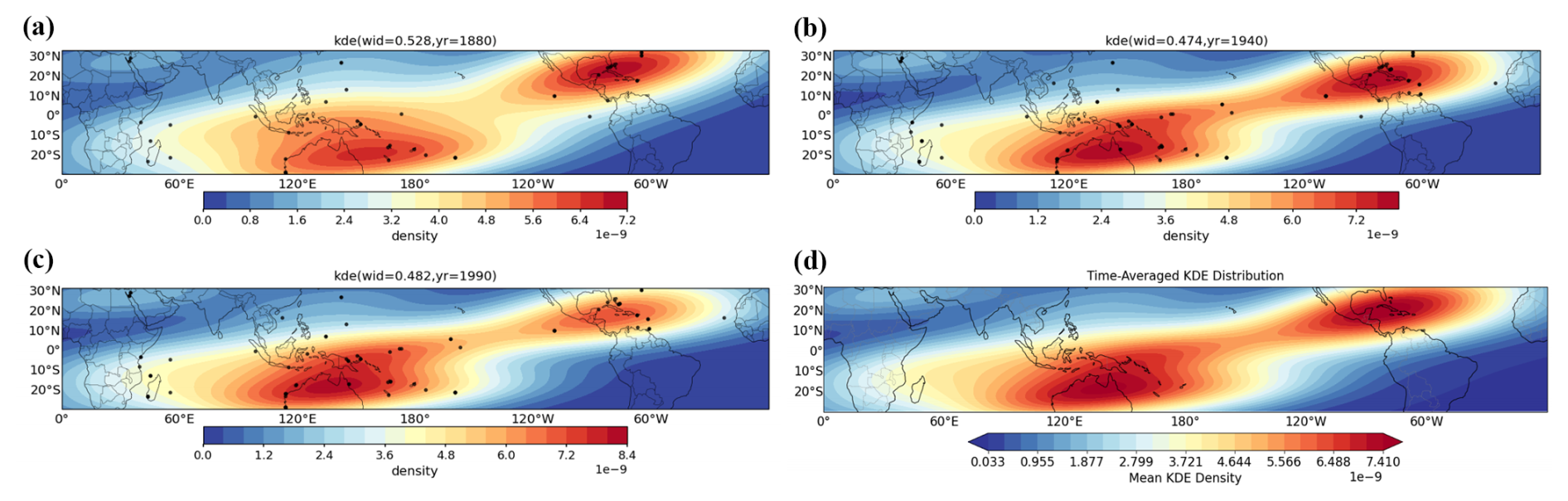
Figure 8 Gaussian kernel density estimation maps for different years: (a) 1880; (b) 1940; (c) 1990; (d) time averaged.

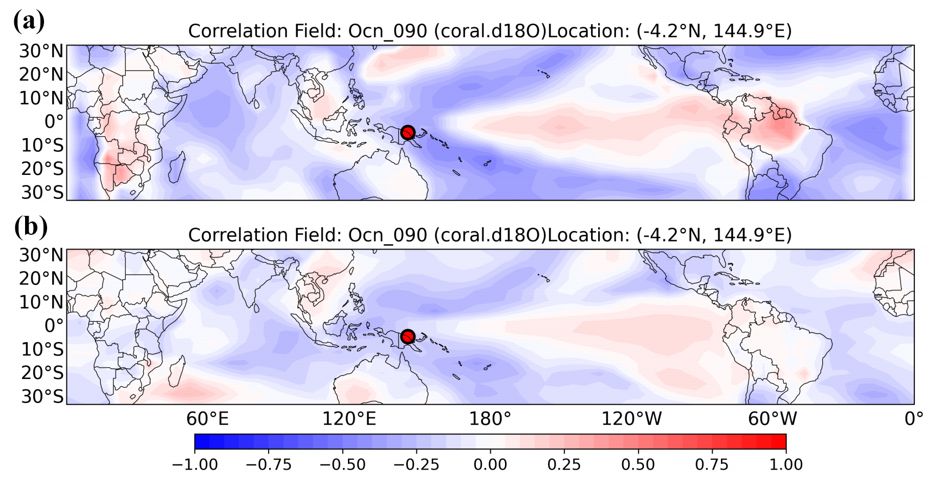
Figure 9 Spatial correlation maps between coral proxy data (ID: Ocn_090) located at 4.2° S, 144° E and (a) instrumental observations, (b) prior data.

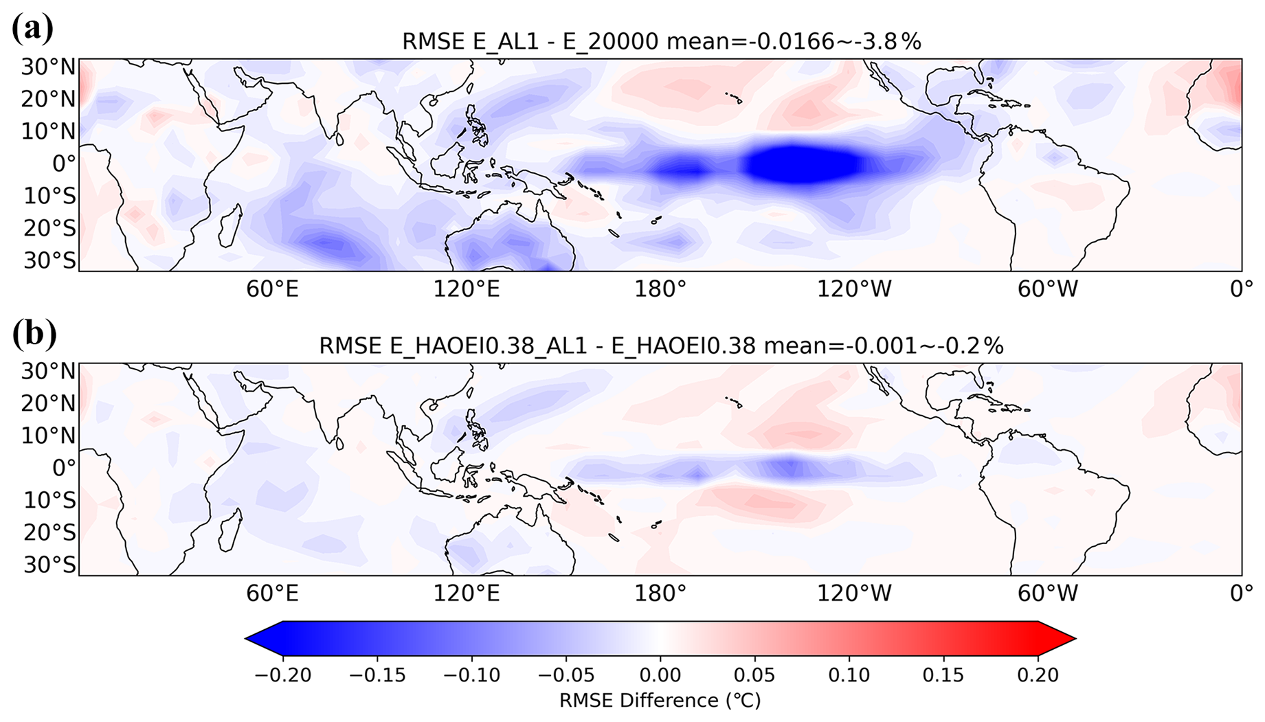
Figure 10 (a) The RMSE differences and the percentage RMSE differences between E_AL1 and E_20000 (b) between E_HAOEI0.38_AL1 and E_HAOEI0.38.

As shown in Figs. 10 and 11, E_AL1 outperforms E_20000, yielding smaller RMSE (E_20000: 0.4377 °C; E_AL1: 0.4211 °C; mean difference = −0.0166 °C, approximately 3.8 %) and generally higher CE (E_20000: −0.2106; E_AL1: −0.1179; mean difference = 0.0927). The improvements scale with data density: moderate in data-rich regions (e.g., Australia, Central America), more substantial in medium-density areas like the equatorial ENSO region, and largely neutral in sparse-data regions such as South America. Similarly, E_HAOEI0.38_AL1 achieves lower RMSE (0.4166 °C) and higher CE (0.1638) than its adaptive-localization counterpart E_HAOEI0.38 (RMSE: 0.4233 °C; CE: 0.1514), indicating that the combination of HAOEI and adaptive localization yields further improvements. Furthermore, Fig. 12 reveals that the leading EOF modes of E_AL1 and E_HAOEI0.38_AL1 exhibit a spatial structure similar to observations but with amplified variability in the ENSO region. Although their explained variance (E_AL1: 42.7 %; E_HAOEI0.38_AL1: ∼ 40 %) remains substantially higher than observed (27.4 %), it is considerably lower than that of E_20000 (66.7 %, Fig. 7), indicating a more faithful representation of the spatial variance distribution. Overall, the application of adaptive localization is beneficial for enhancing reconstruction quality, both in terms of statistical accuracy and the fidelity of dominant climate modes.

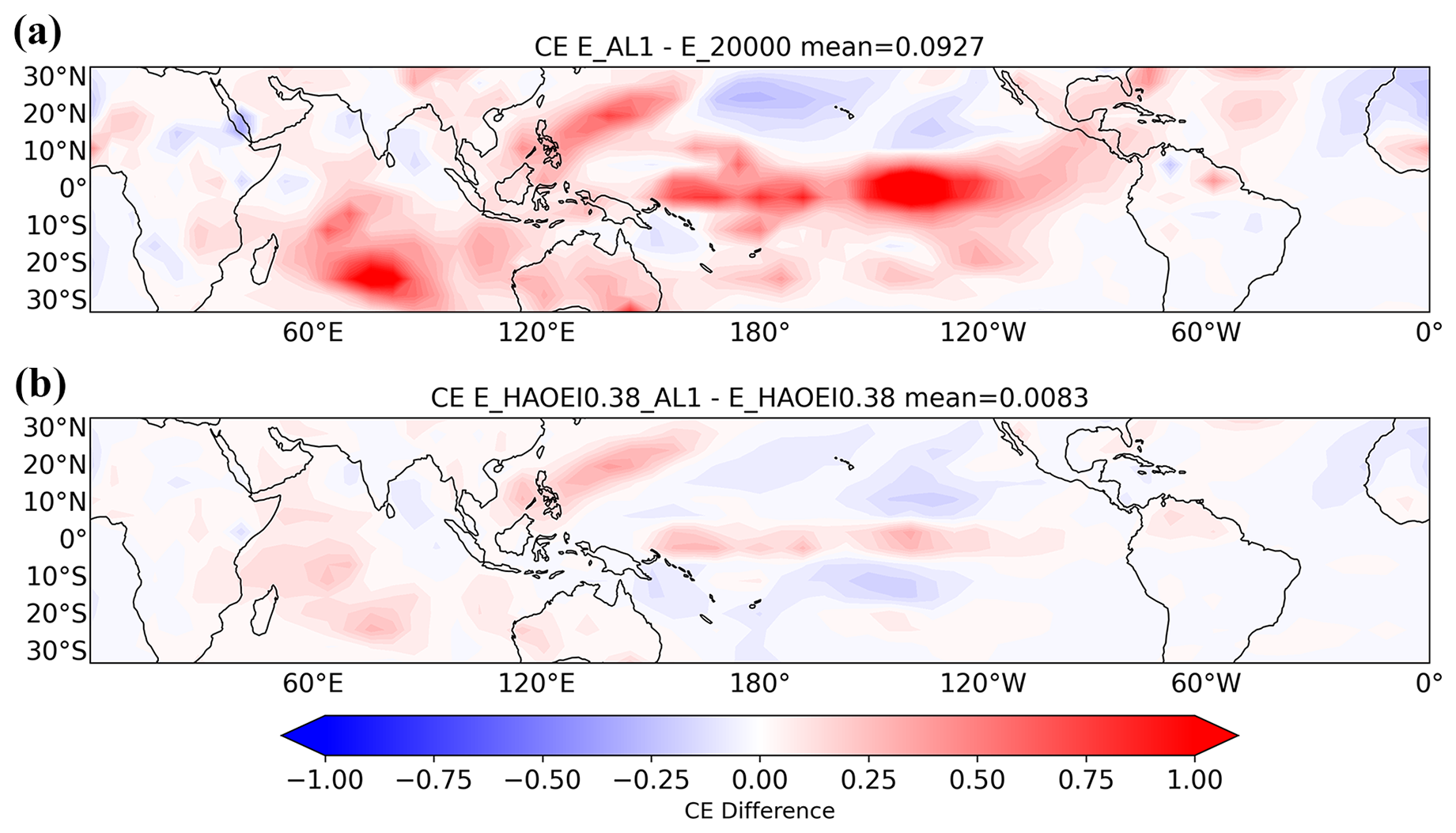
Figure 11 Same as Fig. 10 but for the CE.

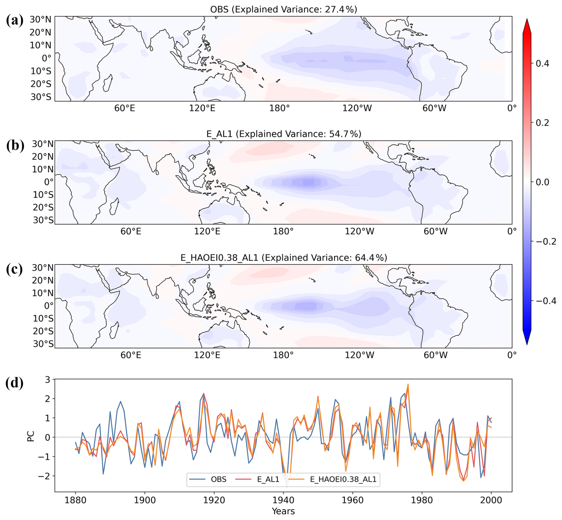
Figure 12 The leading EOF mode of (a) observations (b) adaptive localization analyses (c) adaptive localization and HAOEI (δ = 0.38) analyses (d) corresponding PC time series for all experiments.

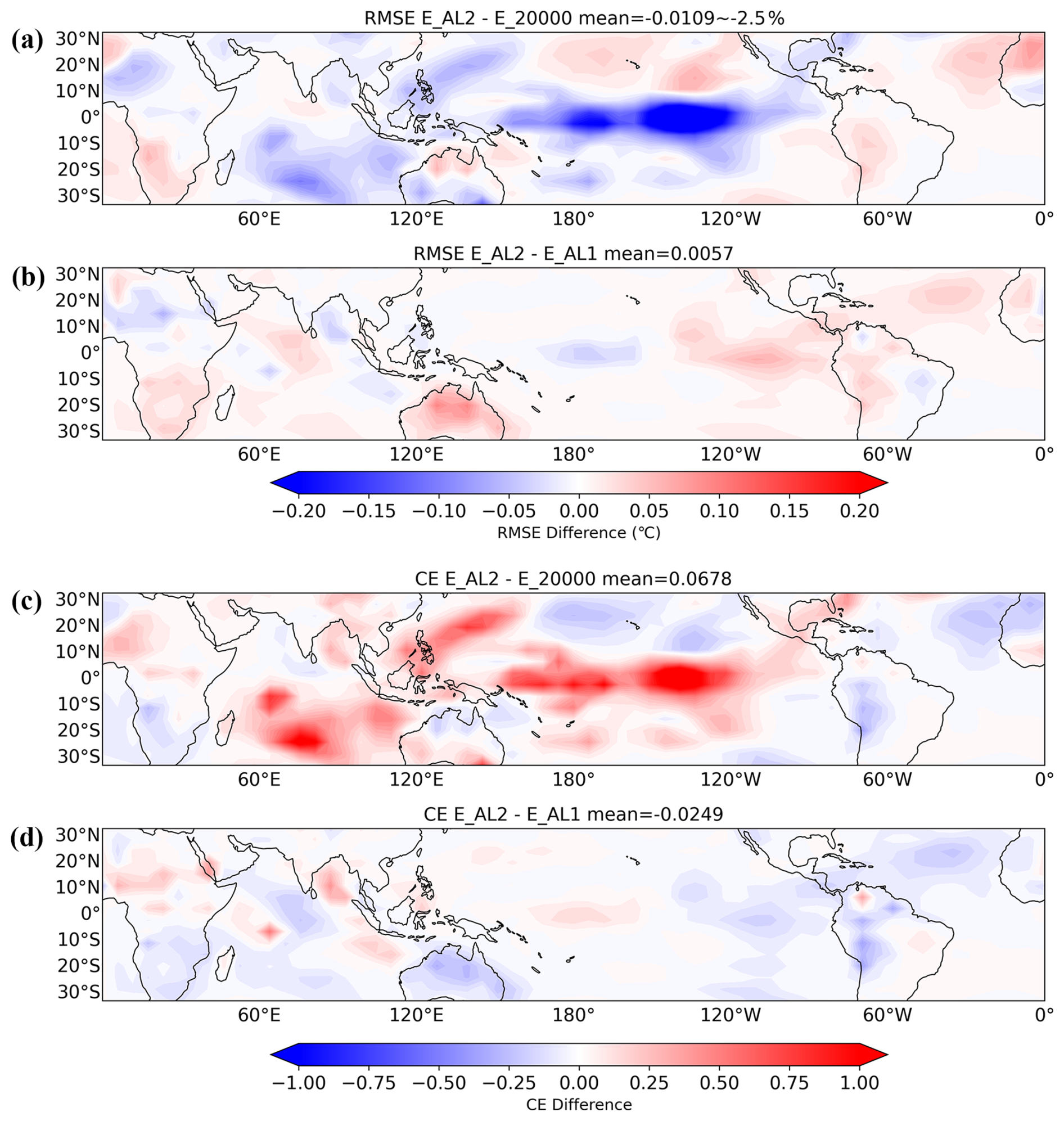
Figure 13 (a) The RMSE differences and the percentage RMSE differences between E_AL2 and E_20000 (b) between E_AL2 and E_AL1 (c) the CE differences between E_AL2 and E_20000 (d) between E_AL2 and E_AL1.

Finally, Fig. 13 illustrates that adaptive localization using model-prior correlations E_AL2 improves upon the fixed-radius baseline E_20000, as evidenced by its lower RMSEs and higher CEs, even if it does not match the performance of the reanalysis-driven version E_AL1. This demonstrates the intrinsic value of the model prior: its physically constrained correlations offer a viable and effective guide for adaptive localization in the absence of reanalysis data. Consequently, this approach ensures the method's applicability to pre-industrial and deeper-time paleoclimate periods, where observational constraints are otherwise unavailable.

4 Conclusion and outlook

This study has developed and systematically evaluated two adaptive strategies within an ensemble-based paleoclimate data assimilation framework: adaptive observation error inflation and adaptive covariance localization. Through sensitivity experiments using coral-based proxy records over the tropical region (1880–2000), we have quantified their impacts on reconstruction quality in terms of pointwise accuracy (RMSE and CE) and fidelity of large-scale climate modes (EOF analysis).

For adaptive observation error inflation, the aggressive AOEI method yields moderate improvements but introduces local degradations where accurate observations are mistakenly down-weighted. The HAOEI method, with its threshold-based linear inflation, provides more balanced and robust performance. Systematic experiments with three δ values (0.67, 0.38, and 0.13) reveal a clear non-monotonic behavior, with δ = 0.38 achieving the largest RMSE reduction (approximately 5.8 %) and the highest CE among all inflation experiments. The existence of an optimal δ indicates a fundamental trade-off: a threshold that is too small over-penalizes moderately inconsistent observations, while a threshold that is too large fails to adequately control genuinely large errors. HAOEI with optimal tuning delivers spatially consistent improvements across most of the tropical domain with substantially fewer local degradations than AOEI.

For covariance localization, the fixed-radius experiments demonstrate that the localization radius critically controls the balance between sampling error and spatial coherence. A large radius preserves large-scale structures but introduces spurious correlations with over-amplified EOF variance, while a small radius distorts the spatial pattern of the leading mode despite yielding a coincidentally close variance percentage. Our proposed adaptive localization method addresses these limitations by dynamically adjusting the radius based on local data density and incorporating correlation-based weights. Compared to the fixed large-radius baseline, adaptive localization reduces RMSE by approximately 3.8 % and substantially improves CE. When combined with HAOEI, the full adaptive system achieves the best overall performance, with the lowest RMSE and highest CE among all experiments. Moreover, the leading EOF modes of the adaptive experiments exhibit spatial structures that closely resemble observations, with explained variances substantially lower than the fixed large-radius experiment and much closer to the observed value. Importantly, the adaptive method remains effective even when correlation information is derived solely from the model prior rather than reanalysis data, confirming its applicability to pre-industrial periods.

In summary, the optimal combination – HAOEI with δ = 0.38 and adaptive localization – yields meaningful improvements in both statistical accuracy and the fidelity of dominant climate modes, reducing RMSE by approximately 5 %–6 % and substantially correcting the over-amplified EOF variance. These improvements, while modest in magnitude, are statistically robust, spatially consistent, and physically meaningful. They demonstrate that the adaptive strategies developed here offer a practical and effective pathway for improving paleoclimate reconstructions, particularly in data-sparse regions and for capturing large-scale climate variability modes such as ENSO.

While this study demonstrates the considerable promise of adaptive strategies in paleoclimate data assimilation, several important avenues merit further investigation to advance the methodology and expand its applications. For the adaptive localization, one could explore time-varying correlation estimates to account for non-stationary teleconnections. Moreover, this study focused on coral-based temperature reconstructions within the tropics; extending the framework to a global scale and to multiple proxy types and climate variables would provide a rigorous test of its generalizability and enable more holistic climate field reconstructions. The methods should be also tested during periods of abrupt climate change (e.g., the Last Glacial Termination, Dansgaard-Oeschger events) or past warm periods (e.g., the Last Interglacial, the Pliocene), where data constraints are particularly challenging but scientific stakes are high.