Advancing the capabilities for efficient hurricane-centric simulations with the atmospheric model ICON

Global storm-resolving simulations with kilometer resolution are increasingly replacing traditional climate modeling approaches and show particular potential for resolving the dynamics and effects of deep moist convection. These modern modeling methods are moving toward sub-km scales, leading to extremely high energy and resource requirements. This makes iterations, parameter optimizations, and sensitivity studies no longer easily feasible. For the class of propagating, large-scale weather phenomena such as hurricanes, high-resolution limited-area approaches in combination with Lagrangian methods are therefore of interest, in which refined grids are shifted along the path of the phenomenon under consideration. To create this capacity for the ICON atmospheric model, this study develops a flexible workflow toolkit to enable efficient simulations of hurricanes on a sub-km scale. Our approach leverages the flexibility that ICON offers through the ability to create custom grids. The concept divides hurricane tracks into overlapping temporal windows of 12–24 h and generates customized grid segments that follow the hurricane's movement. The technical implementation automates key components of the workflow, including hurricane tracking, flexible grid generation, and preparation and merging of initial conditions across successive segments. The application of the workflow is demonstrated using Hurricane Paulette (2020) as an example, for which high-resolution simulations with grid spacings down to 300 m were performed using different segment configurations. The results show that the hurricane track remains consistent with the base run and depends mainly on the across-track width of the chosen configuration, while intensity metrics such as minimum pressure and maximum wind speed show significant sensitivities to resolution in our multi-nested setups. The efficiency gains are significant compared to traditional approaches with fixed limited-area domains: replacing a fixed domain with a track-following tube reduces resource requirements by factors of 2–8, and segmenting the tube into short, frequently re-initialized intervals adds a further factor of 2–6. Analysis of re-initialization effects shows systematic but manageable impacts during segment transitions. Nevertheless, the efficiency gains achieved by our method are so substantial that they justify the acceptance of the re-initialization effects. Our segment-based approach in the hurricane-centric reference system now allows for more flexible regional hurricane simulations with the ICON model and more efficient investigation of new research questions regarding the sensitivity of hurricane cloud systems at very high resolutions.

1 Introduction

Global storm-resolving simulations on a kilometer scale are increasingly replacing traditional climate modeling approaches (Satoh et al., 2018, 2019; Segura et al., 2025). These modern modeling methods show particular potential for resolving the dynamics of deep moist convective phenomena and their various forms of spatial organization, and the resulting interactions between small and large scales in a more physically realistic manner. Global storm-resolving simulations are now constantly evolving from kilometer to hectometer resolutions, enabling unprecedented detail in the representation of atmospheric processes (Hohenegger et al., 2023; Klocke et al., 2025). However, the development and calibration of these high-resolution approaches pose significant challenges (Shukla et al., 2010). They are extremely energy- and resource-intensive in terms of both computing resources and storage requirements. As a result, iterations, parameter optimizations, and sensitivity studies can no longer be easily performed (Mauritsen et al., 2022). For this reason, alternative and efficient approaches are needed to understand how well regional to locally limited phenomena are represented at high resolutions and standard parameter settings.

One typical solution to this problem is to use limited-area domains with high spatial resolution that refine the global model simulations in a predefined limited area and within a certain time period, thereby significantly reducing the computing resources required. These limited-area solutions can be designed to be consistent with global simulations by using initial and boundary conditions derived from them and working with the same set of physical parameterizations. Of course, the capability of limited-area approaches is inherently somewhat constrained, since interactions with boundary conditions can introduce errors and the upscale influence of small-scale processes onto the larger scales is not captured adequately. The atmospheric component of the Earth system model ICON (ICOsahedral Nonhydrostatic, see Zängl et al., 2014) already includes the possibility of simulating such regional domains with nested grid refinements (Stevens et al., 2020; Zängl et al., 2022; Hohenegger et al., 2023). These approaches are usually limited to spatially fixed domains that must be defined in advance. This concept is very well suited for spatially and temporally limited phenomena, such as the diurnal evolution of convection over land under rather calm wind conditions. However, the approach with fixed regional domains is less suitable when the weather phenomena under consideration propagate over large distances, such as hurricanes, and thus the covered area is as large as entire oceans. For this class of problems, high resolution Lagrangian approaches are interesting, in which the refined grids are shifted along the path of the phenomenon under consideration. Such approaches have been successfully applied for a long time for flexible high resolution hurricane forecasts in operational settings (Kurihara et al., 1998; Gopalakrishnan et al., 2002).

For predicting the path of hurricanes, km-scale model approaches have been shown to reach reduced track position errors (Dong et al., 2020). For accurate simulations of the structure and intensity of hurricanes, an explicit and well-designed representation of deep moist convective processes also appears to be key (Gao et al., 2023). It has been further shown for Hurricane Katrina, that its intensification and structure of its convective bands only improved sufficiently when a spatial resolution of around 1 km is achieved (Davis et al., 2008). Systematic investigations in Davis et al. (2011) have also shown that intensity biases with resolutions around 1 km are reduced, especially for very high wind speeds, compared to coarser model resolutions. The study argues that it is essential to resolve cloud structures in hurricanes, but also that significant improvements between 100 m and 1 km horizontal resolution are questionable. These examples can be continued and provide evidence that a high spatial resolution is essential for realistic hurricane simulations and that entering the sub-kilometer scale may need further investigations.

Together, high spatial resolution and flexible adaptation of simulation domains can help enable novel, high-quality hurricane simulations while keeping computing costs within reasonable limits. Our efficient approach presented here contributes to this goal and advances the capabilities of ICON model. Redesigning the grid and data management in ICON and the associated communication patterns is so challenging, and the risks of negatively impacting the outstanding performance achieved in Klocke et al. (2025) are so high, that we have decided to implement a workflow-based approach to make regional hurricane simulations more flexible. This approach is an intermediate step on the way to a fully Lagrangian model concept and has the advantage that we can completely retain the proven and optimized communication patterns and data structures of ICON. Our approach allows us to take advantage of the flexibility that ICON offers through its ability to create user-defined grids. In this way, we can perform targeted and efficient hurricane-centric simulations down to the hectometer scale without having to re-optimize the efficiency of the underlying model. We are thus creating the possibility of using an approximate Lagrangian approach with the ICON versions available today to create innovative datasets for hurricane investigations in very high resolution. With this approach, we would like to encourage the scientific modeling community in general to give more consideration to co-design methods that promote the parallel development of sophisticated global simulation approaches and flexible and efficient regional refinements.

The paper is structured as follows: In Sect. 2, we present the methodology of our flexible refinement workflow in detail. We provide a conceptual overview together with detailed workflow diagrams and discuss the portability of our methods to different high-performance computing platforms. Section 3 demonstrates the application of the workflow using Hurricane Paulette (2020) as an example. Different refinement strategies are explored, and the results of high-resolution simulations are presented and discussed. There we also provide an analysis of the performance and resource requirements of our approach. Finally, Sect. 4 summarizes the key findings and outlines potential future directions for research in this area.

2 Methodology

2.1 General Overview

Figure 1 provides a general overview of the flexible refinement workflow used to create high-resolution hurricane simulations. The various steps are carried out sequentially. The first step is to create a base simulation of a hurricane. Both global and sufficiently large regional setups can be used for this purpose. In the example case presented in Sect. 3.1, a limited-area setup covering the entire tropical Atlantic is employed. Global storm-resolving simulations, such as the projections of the nextGEMS project (Segura et al., 2025), could also be used as base simulations. A wide range of data from the base simulation will be required in subsequent steps.

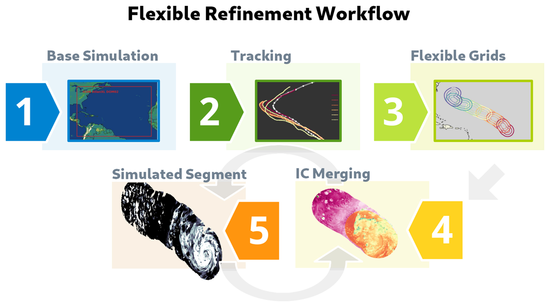
Figure 1 Overview of the flexible refinement workflow: Five steps are shown in different colored boxes and numbered accordingly. The steps of the workflow include (1) creating the base simulation, (2) identifying and tracking the hurricane, (3) creating the flexible grids and other necessary simulation data, (4) combining the initial conditions from the base and newly created simulation data, and (5) performing the actual high-resolution hurricane simulation. Gray arrows indicate the flow in the workflow diagram, with steps 4 and 5 being performed as iterative loop over the respective hurricane segments.

An important prerequisite is that the base simulation generates a hurricane and reproduces its characteristics sufficiently well. In the second step (see Fig. 1), the hurricane is identified in the base data and tracked over time. This tracking process creates a Lagrangian reference system, initiating the transition from a fixed domain to a flexible, hurricane-centric setup. It is important to note that we follow the hurricane as a large-scale structure which is not necessarily the same as shifting the domain according to the mean horizontal wind.

In the third step, we split apart the hurricane track into individual elements, which we refer to as “segments”. Based on these, flexible and user-defined grids are set up that overlap so that previous information can be used for subsequent simulations. All essential data like external parameters, lateral boundary and initial conditions (ICs) are created specifically for these grids. This completes the pre-processing workflow.

Steps four and five build the production workflow. Both steps are performed alternately for each simulation segment. Step four generates the respective ICs from which the atmospheric simulation is started. For the first segment, ICs are created solely from the base simulation. Step five conducts the actual high-resolution hurricane simulations in the respective grid segment and stores the necessary ICs for the next simulation. For the second and the subsequent segments, the loop goes back to step four and data from the previous segment is reused in the overlap area for the new simulation. Where there is no overlap between two subsequent grid segments, ICs from the base simulation are taken. Thus, step four produces a mixed initial state consisting of a merge of two information sources (see Sect. 2.3 for more details).

2.2 Segment Concept

Our entire workflow is based on the idea of simulating a hurricane only within its vicinity along its temporal evolution. To accomplish this efficiently, we rely on a segment concept for which a reference track is divided into individual track segments. The length of the track segments is mainly determined by the envisioned re-initialization time interval, Δt_reinit (plus some additional buffer). Re-initialization data must be available from the base simulation for the chosen interval, e.g. 12 or 24 h, to support the re-initialization of the higher-resolution simulations.

Figure 2 shows how a track segment is constructed. The points B and C correspond to the location of the hurricane center in the base simulations at times t₀ and t₀+Δt_reinit. The points A and D expand the track segment in the respective directions by a certain buffer distance to account for situations in which the hurricane moves slower or faster along its path in the higher-resolution simulations. For practical reasons, this buffer distance is also specified as a time interval, Δt_add. Combining re-initialization interval and buffer time, the selected track segment runs from point A to point D and thus covers the distance traveled by the hurricane e.g., from 21:00 UTC the previous day to 15:00 UTC (Δt_add=3 h; Δt_reinit=12 h).

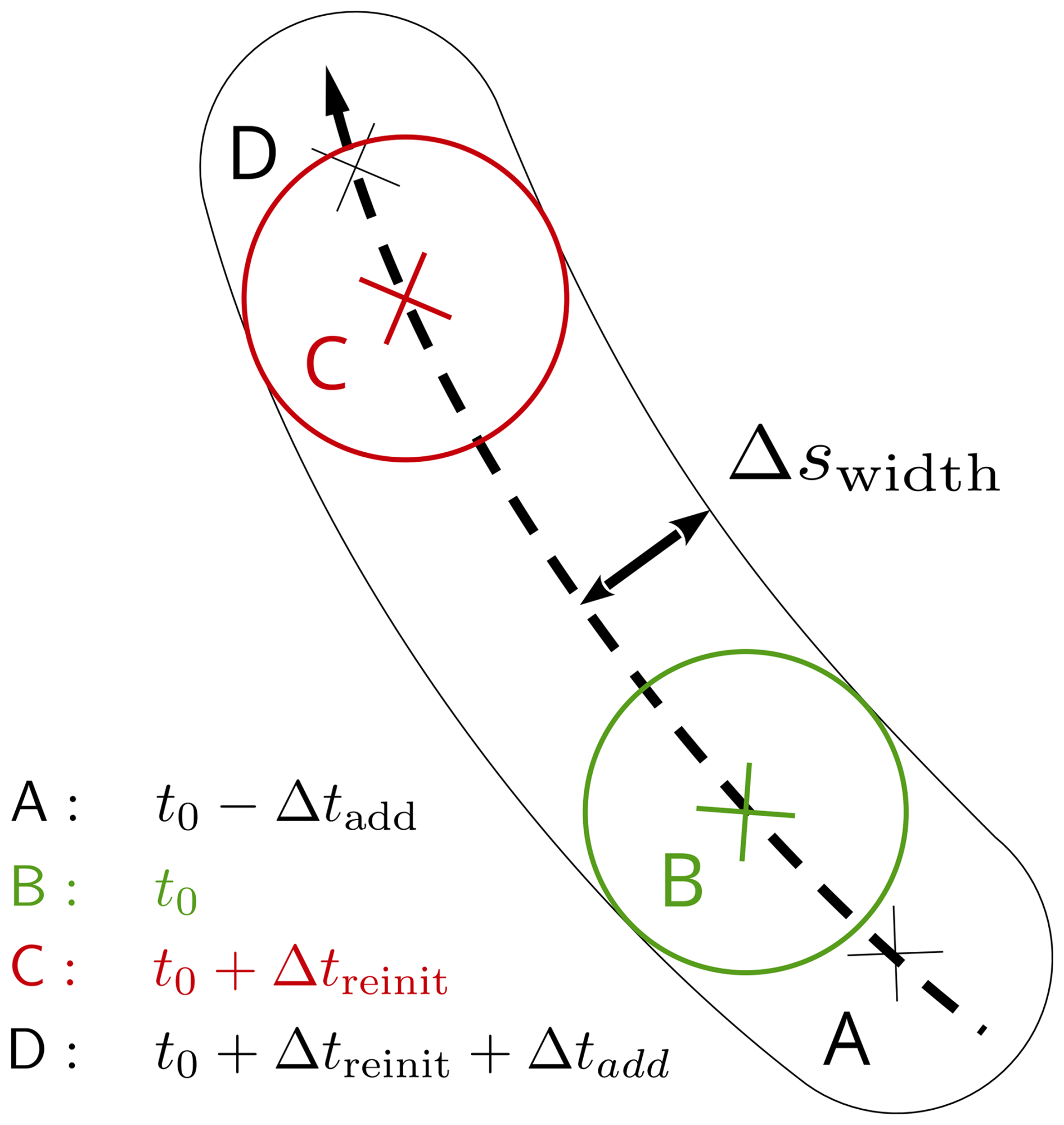
Figure 2 Schematic representation of a track segment. The reference track is represented by a thick, dashed black line. A grid segment with a width of Δs_width is constructed around it (thin solid black line). The spatial points A to D are determined by their temporal sequence along the track. The circles around points B and C indicate the areas of interest for analysis at the start and end time of the simulation within the segment. Points A and D show the extension of the grid segment by a predefined time Δt_add. For simplicity, only the outer nest of the track segment is shown. Further nests follow the same scheme, but lie inside the outer nest with smaller across-track widths.

A grid segment refers to a track segment that has been spatially expanded horizontally. It is constructed by expanding the selected track segment by a user-defined across-track width, Δs_width, in all directions, forming a tube-like shape. Imagine a circular area with a radius of Δs_width and the center at the respective track point sweeping over the track segment. The circular section at a time t is defined later as Lagrangian analysis region for more detailed investigations (see Sect. 3.4).

Finally, the segment concept is applied to different start times t_i which link the kth segment to an individual initialization time. For practical reasons, we count segments in relation to the initialization time of the reference t_ini. The start time of the kth segment is thus given by $t_k=t_{\text{ini}}+k\mathrm{\Delta }{t}_{\text{reinit}}$ where k=0 selects t₀=t_ini. If e.g. 24 h of model spin-up are omitted from the reference data, the first meaningful segments can be found at k=1 for Δt_reinit=24 h and at k=2 for Δt_reinit=12 h. However, it is up to the user to define which segments are the first meaningful segments in their simulation chain.

2.3 Workflow Schemes and Implementation Details

Section 2.1 provides an introductory description of the various stages incorporated within the workflow. Specifically, steps 1 through 3 are categorized under the pre-processing workflow, while steps 4 and 5 pertain to the production workflow. The automation of tasks using algorithms exhibits varying degrees of complexity. In the following, a detailed analysis is shown that details the implementation of the most complex algorithms used throughout the workflow.

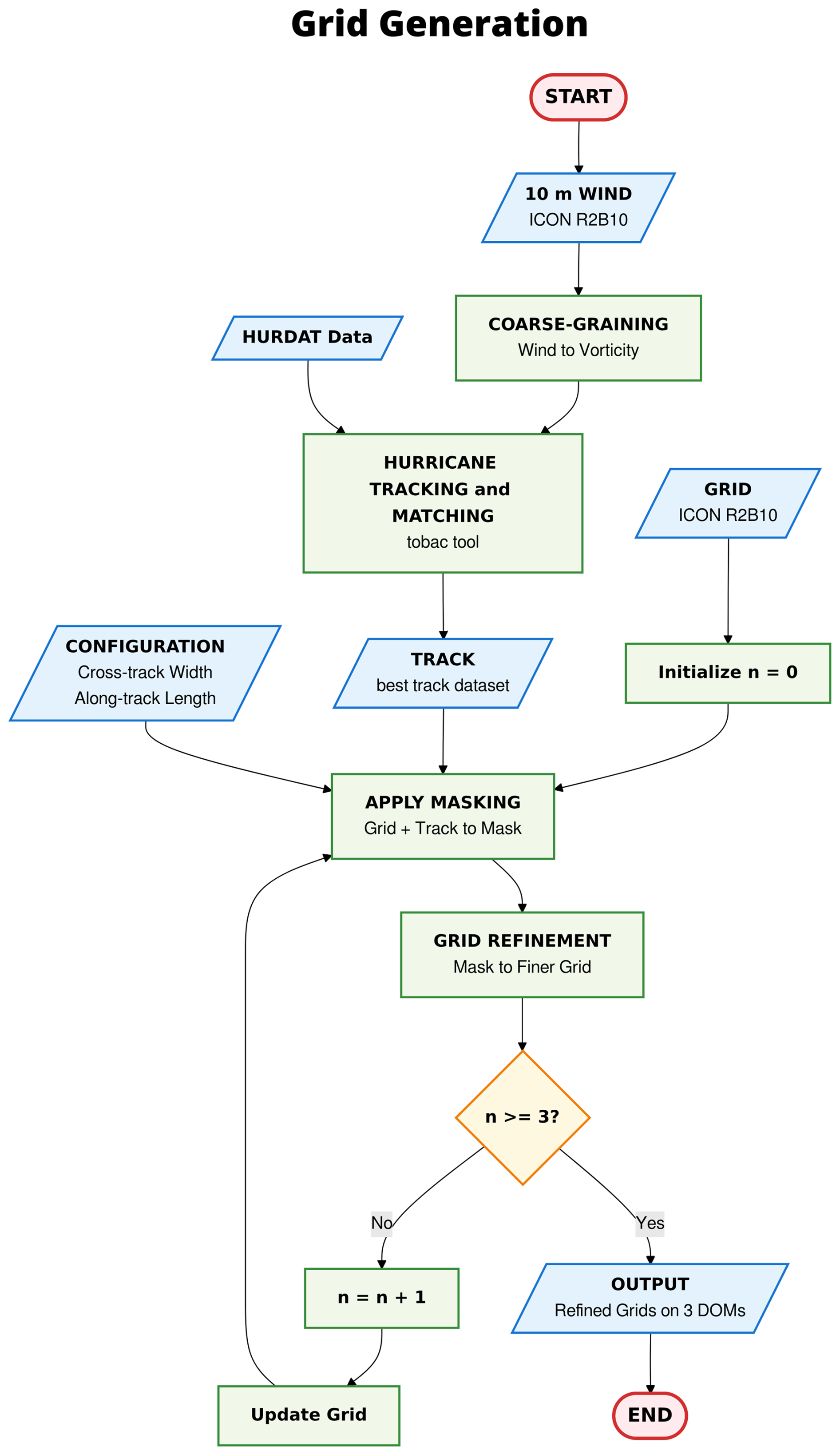
Figure 3 Detailed flowchart for the sequential grid generation process. Final start and end points are highlighted in red. Incoming and outgoing data are visualized as slanted blue boxes and methods that treat these data are shown as green rectangles. The index n counts the number of nested domains and thus determines the number of iterations in the grid generation loop. The term R2B10 indicates the triangular grid configuration of the ICON base run with a grid spacing of approximately 2.5 km.

Figure 3 provides a comprehensive flowchart of the grid generation algorithm. The starting point is the horizontal wind field at 10 m height from the base simulation that is converted to relative horizontal vorticity ζ and further coarse-grained with a running-average filter with a width of around 200 km. The coarse-grained vorticity ζ_c field allows to identify larger-scale cyclonic motions such as those characteristic for hurricanes. Detection and tracking of cyclonic features is done with the open-source python package tobac (Heikenfeld et al., 2019; Sokolowsky et al., 2024). A threshold criterion of ${\mathit{\zeta }}_{\mathrm{c}}=\mathrm{10}{\mathrm{d}}^{-\mathrm{1}}$ was used for identification, ensuring only the strongest motions were selected. Please note that a variety of other and more customized tools are available for identifying and tracking hurricanes, such as TempestExtremes (Ullrich et al., 2021) or the approaches by Kleppek et al. (2008) and Enz et al. (2023), which could have been applied here with equal justification. The preparation of the hurricane track data from base simulations is concluded by a matching algorithm. It utilizes location data of past hurricanes from HURDAT (Landsea and Franklin, 2013) to find the closest matching hurricane track in the base simulations (similar to Gutmann et al., 2018). This use of observational best-track data only provides additional insights for nudged simulations or simulations in a forecast mode, for free-running climate simulations a comparison to the observational track may not be physically meaningful.

The actual grid generation loop is entered with data from the best matching track, from a base grid (here, we take the grid from the finest reference nest) and from a configuration file that allows users to specify the along- and cross-track extend of the grid segments. The grid generation algorithm relies on DWD-ICON-Tools software (see Zängl et al., 2022, for grid-related aspects), facilitating the creation of flexible ICON grids through masks, crucial for our hurricane-centric workflow. For masking, a chosen base grid is read. Then, the track segment and its spatial extension by the across-track width, Δs_width, are transferred to this grid to create a mask. The resulting mask is then used in the DWD-ICON-Tools grid generator to create the next refinement cutting out only the chosen grid segment. This builds the outermost nest of a flexible setup and serves as the basis for further refinements. If multiple nests are targeted, the track segment is transferred again, now to the just created outermost nest, and the lateral extension is performed again with a predefined, but smaller across-track width. This process is repeated several times until all nests for the respective refinement levels have been created. In Fig. 3, the shown loop determination criteria is n=3 which means that a sequence of three nested grids with successively halved grid spacing are created. Finally, these nested grids resemble layers of an onion.

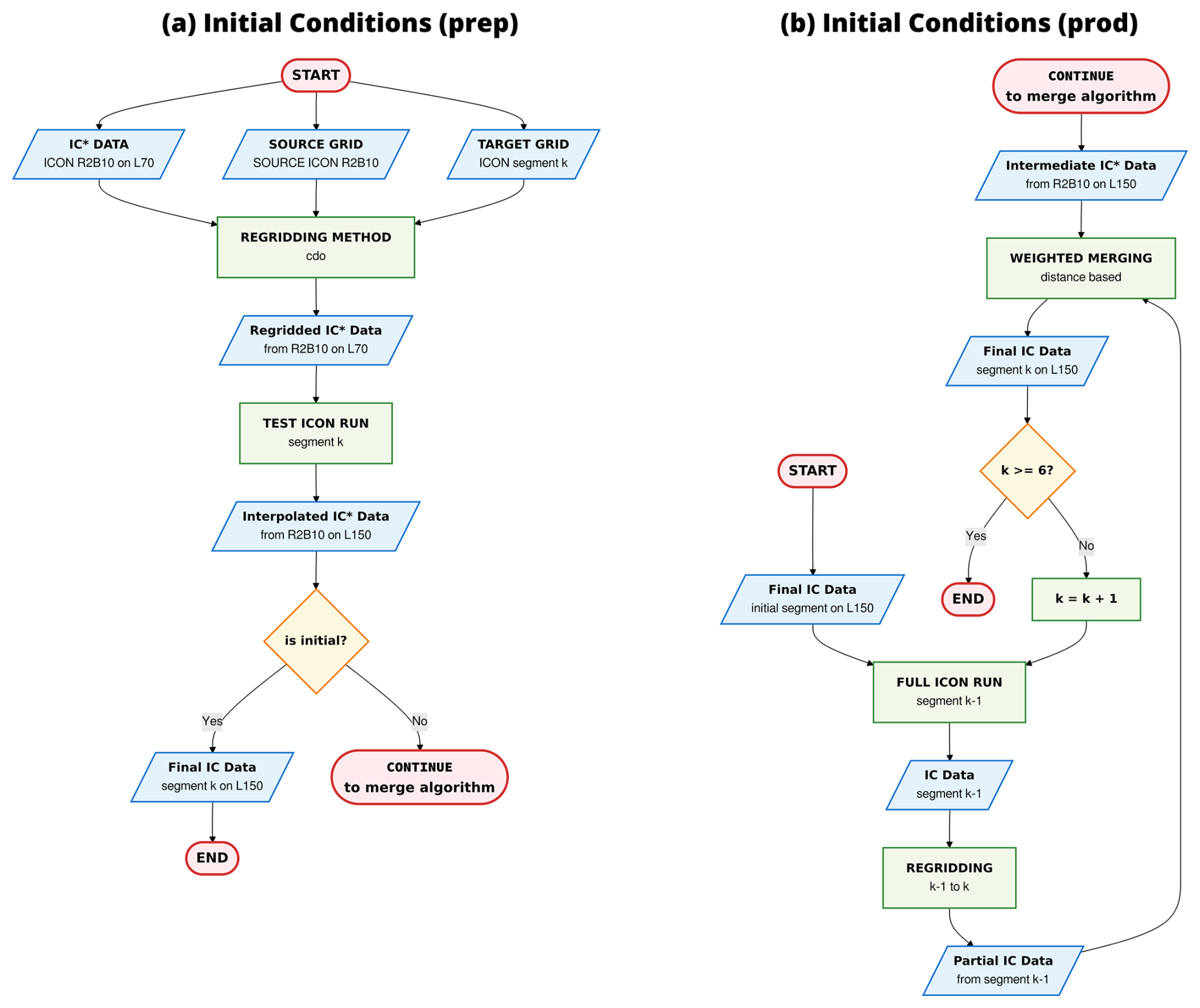
Figure 4 Detailed flowchart for (a) initial conditions pre-processing and (b) initial conditions production. Final and intermediate start and end points are highlighted in red. See Fig. 3 for meaning of the other elements. The index k counts the number of segments along the hurricane track. The loop terminates after a user-defined number of segments, e.g. here k=6. The term L70 (L150) indicates the vertical grid configuration of the ICON base run with 70 (150) vertical levels.

Figures 4a and b split up the automated algorithm for IC generation into a pre-processing part and into a production part. For IC pre-processing, data from the base simulation, here noted by IC^* as well as reference grid (source) and segment grid (target) are input. The horizontal regridding uses the tool cdo (Schulzweida, 2023) together with a conservative remapping to calculate regridded IC^*. This dataset is input into a test ICON run that serves several purposes. With the test run (i) the integrity of the execution workflow is tested, (ii) performance-relevant aspects are investigated and resources for production runs are estimated and (iii) internal vertical interpolation is applied to consistently bring the regridded IC^* from the reference levels to the possibly more refined target levels. After that point, the IC pre-processing workflow stops with the decision whether the considered segment is chosen to be the initial segment or not.

In the IC production chain, regridded IC^* are input into the full ICON run for the initial segment. At the end of the successful full ICON run, IC data for initializing the next segment are stored. Due to along-track shifts of the grid segments, these IC data only partially cover the region of the next segment. To compensate for this offset, a merging algorithm is applied that maps the partial IC data from segment k−1 to the grid for segment k in the overlap area. The remaining parts are filled with regridded IC^* from the reference. The transition between the two IC data sources is smoothed by weights that decrease linearly with distance from the overlap boundary. Still, the mix of two IC datasets introduces a discontinuity in the initialization - a limitation that is discussed in depth in Sect. 3.5.

After grid and IC generation, the external parameters and boundary conditions are remapped onto the newly created grid segments. The former is directly interpolated from the original external data onto the respective grids yielding the highest possible resolution of e.g. topography. The latter is exclusively obtained from the base run data and mapped using cdo on the respective lateral-boundary grids of the high-resolution simulations.

2.4 Portability and User Interfaces

The workflow toolkit is intended to run on super-computing platforms. It consists of a mix of python tools and bash scripts, the latter being submitted into a HPC scheduling system. The workflow was initially developed for the German Climate Computing Center (DKRZ) and its computing platform Levante and adjusted to its specific module environment and the Simple Linux Utility for Resource Management (SLURM) scheduler. The toolkit was then ported to the Jülich Supercomputing Center (JSC) Platform JUWELS, and its most important aspects were generalized. We therefore consider the software to be relatively platform-independent. In order to port the workflow toolkit, only the configurations of the corresponding module environment and the SLURM schedulers need to be properly set up for new platforms.

Users can readily configure the toolkit via a detailed configuration file, allowing them to set and modify parameters, as well as file and software dependencies, for different numerical experiments. We chose a TOML (Tom's Obvious, Minimal Language)-based configuration containing clearly structured elements and sections that can be easily edited with standard text editors. Additionally, we provide wrapper scripts to initiate the execution of entire workflows. It is possible, on the one hand, to start the pre-processing workflows of an entire series of consecutive grid segments. This results in the parallel execution of individual workflows that carefully handle their internal sequential dependencies. On the other hand, the production workflow wrappers can be executed. These trigger the execution of the ICON model in the selected grid segment with multiple restarts, if necessary, and merge the ICs before starting an ICON run for the next segment. All other user-relevant information can be found in the documentation of the latest software release (Senf, 2026c).

3 Application

3.1 Case Description

We now introduce a hurricane case chosen for demonstrating our flexible refinement workflow for hurricane-centric high resolution simulations. In 2020, Hurricane Paulette crossed the Atlantic and, with a total length of around 11 400 km, was one of the hurricanes with the longest track for that year. According to the National Hurricane Center's tropical cyclone report, Paulette formed as a tropical depression in the central Atlantic on 7 September and intensified into a tropical storm as it moved northwestward (National Hurricane Center, 2021). It reached category 1 hurricane status on 13 September, intensified further into a category 2 hurricane in the early hours of 14 September, and reached peak intensity of 90 kt (46 m s⁻¹) and 965 hPa around 18:00 UTC on 14 September. A snapshot of Paulette during its most intense phase is shown in Fig. 5a. Paulette finally transitioned into an extratropical cyclone at 12:00 UTC on 16 September. During its first seven days of formation and main intensification period, Paulette's path was relatively straight, making it an ideal use case for our workflow methods.

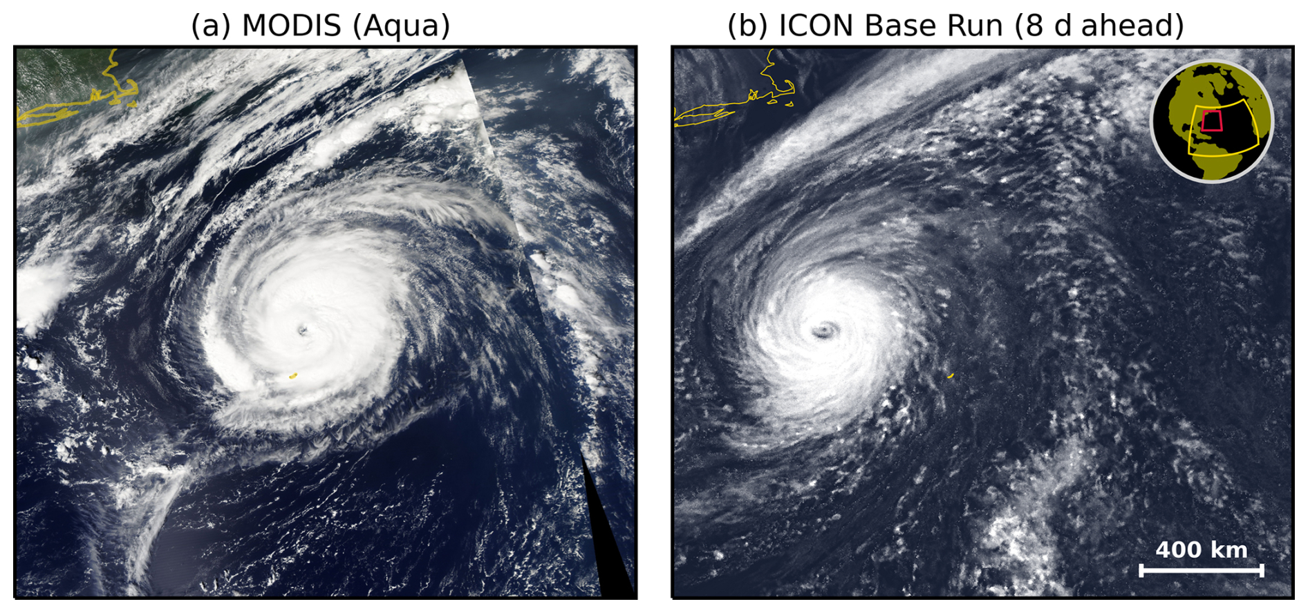
Figure 5 Top view of hurricane Paulette from (a) observations and (b) simulations. A regional cutout in the Atlantic ocean was defined reaching from −74.0 to −53.4° E and from 25.0–43.2° N. Subpanel (a) shows a true-colour image acquired by the Moderate Resolution Imaging Spectroradiometer (MODIS) instrument on the NOAA-AQUA satellite during an ascending orbit at overpass time on 14 September 2020, around 18:00 UTC. Subpanel (b) provides a simulation of the reflected solar radiation flux, normalized between 100 and 750 W m⁻² from our ICON base run, which was initialized on 7 September 2020 at 00:00 UTC. The time, geographical region and projection have been matched between the observation and the simulation. The color scale and map in (b) have been adjusted to ensure visual consistency with (a). The length scale of 400 km is shown in the lower right corner of (b) and the inset in the upper right corner of (b) shows the location of the image cutout (red outline) and the inner base run domain (yellow outline) in the Atlantic ocean. MODIS imagery by NASA.

3.2 Base ICON Run

The ICON model solves hydrodynamic equations on a triangular grid (see Zängl et al., 2014; Dipankar et al., 2015), and can operate as a global or regional modeling system (Hohenegger et al., 2023; Müller et al., 2025). For our baseline run, we used the regional setup of the ICON model in the configuration with the numerical weather forecast (NWP) physics package (Zängl et al., 2014). The base simulations with an outer limited-area setup and grid spacings of 5 km forced by ERA5 data (Hersbach et al., 2020) were performed into which a second, inner domain with 2.5 km grid spacing was nested using one-way coupling.

For the outer nest, a spatial extent of 9900×6700 km² was chosen, which covers most of the tropical and subtropical Atlantic north of the equator. The outer nest was configured as R2B9 triangular ICON grid, corresponding to an equivalent grid spacing of 5 km. In this domain, convection processes and convective precipitation were parameterized following Bechtold et al. (2008) based on Tiedtke (1989). For the inner nest, the ICON R2B10 grid setup was chosen, corresponding to a grid spacing of approximately 2.5 km. The vertical resolution of the base run was set to 70 model levels in both nests, extending from sea surface to a maximum height of 34 km. The inner nest is driven by the outer nest via a nudging zone close to the lateral boundary. However, due to one-way coupling, the inner nest does not provide feedback to the outer nest. In the inner nest, subgrid-scale convection was partially parameterized. The resolved model dynamics explicitly represent deep convective processes, while a parameterization approach still approximates shallow to mid-level convection. This setup has been shown to sufficiently reproduce realistic marine cloud structures and cloud radiative effects (Senf et al., 2020).

All other parameterizations from the NWP physics package were selected identically for both setups. Thus, all ICON simulations used the two-moment cloud microphysics scheme after Seifert and Beheng (2006). Subgrid-scale turbulent fluxes were calculated using a closure approach, as described by Baldauf et al. (2011), which includes the prognostic calculation of turbulent kinetic energy. The scheme ecRad was used for radiation calculations (Hogan and Bozzo, 2018). It performs radiative calculations in 14 solar and 16 terrestrial pre-defined spectral bands.

The simulations utilized in the following were initialized at 00:00 UTC on 7 September using the ERA5 data, a reanalysis dataset produced by European Centre for Medium-Range Weather Forecasts (ECWMF, Hersbach et al., 2020). This corresponds to a time when Paulette had already developed into a tropical depression. ERA5 data is available six-hourly as boundary data for the outer nest. For the base run, ICON version v2.6.6 is selected, which was the most recent ICON version at the time the base simulations were created. On top of this version, an update was developed that allows the sea surface temperature from ERA5 to be updated daily for all regional nests (Senf, 2026a). Therefore, SST fields are not kept constant at the initial SST values, but changed on a daily basis for our hurricane base simulations. Consequently, the actual effects of Paulette on the ocean surface are already included, which could indeed negatively impact the quality of simulating the hurricane development (Bender and Ginis, 2000). The output of the base run was configured so that data for initialization or re-initialization of higher-resolution runs is available every six hours. Furthermore, data to drive high-resolution runs via lateral boundary conditions is available at a resolution of one hour.

Figure 5b shows a visual impression of Hurricane Paulette simulated with our base run setup, at the time of the most intense hurricane period. The figure shows the reflected solar radiation at the top of the atmosphere for the inner R2B10 nest after an integration time of around eight days. For operational forecasts, Gao et al. (2023) reported a mean track error of approximately 300 km after 5 d of lead time. Here, a distance of approximately 400 km between our simulated hurricane center and the observation is achieved, which is a very positive result for a hindcast with around 8 d of lead time. Given the complexity and multiple interacting processes involved in hurricane formation, the reasonably good agreement was somewhat unexpected for the rather long forecast lead time. Although the variables being compared between the observation and simulation are not the same, making a quantitative comparison difficult, we still observe interesting differences in the morphology of the simulated hurricane compared to the observation. It appears that the spatial extent of the simulated anvil cloud associated with the hurricane is underestimated. Insufficient spatial resolution could be one reason for this discrepancy, among many others, and methods that lead to more spatially refined simulations, such as the workflow presented in this paper, would be an important step in further investigating this question of resolution dependence.

3.3 Exploration of Different Refinement Strategies

In the following, we will examine the refinement workflow presented in Sect. 2 in more detail for Hurricane Paulette as an example. As shown previously, the base run results reveal an intriguing hurricane development, motivating us to conduct further investigations with higher resolutions. This is exactly the starting point for the flexible refinement workflow presented in this paper. The base data is now entered into the flexible grid calculation alongside the calculated track of the simulated hurricane.

As a user, one can now choose from various important parameters. These parameters determine how many grid segments are created and their size. The first fundamental question concerns the spatial resolution. Starting with the resolution of the base run (R2B10 with 2.5 km), higher resolutions can be achieved through successive refinement. The following example uses setups with three nests, ranging from R2B11 with a grid spacing of 1.2 km to R2B13 with a grid spacing of approximately 300 m. The currently implemented workflow can handle fewer nests but would require additional software updates for using more than three nests. In principle, it is also possible to start initial refinement from grids finer than the base grid for which minor software updates would be needed.

Figure 6 shows various implementations of grid segmentations for Paulette. These implementations vary either the length of a segment along the hurricane track (white line) using the “reinit” parameter Δt_reinit or the across-track width Δs_width. The different grid segments are visualized by different colors. When Δt_reinit=12 h is selected (Fig. 6a and c), the grid segments appear shorter and more compact. However, more grid segments must be calculated sequentially to cover the same integration period. For the 12 h re-initialization setup, it makes sense to start with segment 2 on 8 September 2020, at 00:00 UTC to avoid spin-up of the base run. If the integration ends after the 12th segment, as shown, the hurricane's development can be tracked for five days and 12 h. The 24 h re-initialization setup requires fewer segments. However, each segment covers a larger region and requires more computing power (see Fig. 6b and d). Each of the 24 h setups shown starts with segment 1, and sequential integration up to segment 6 covers a period of six days.

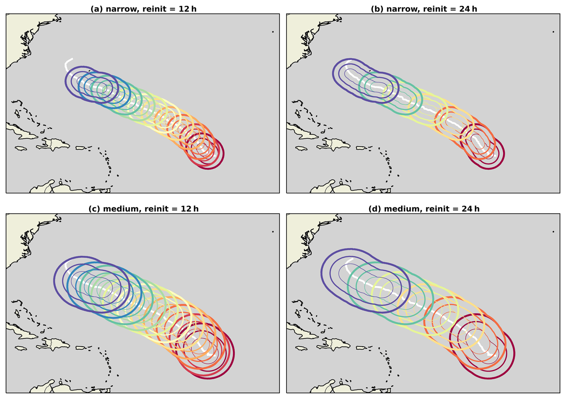
Figure 6 Grid segments prepared for hurricane Paulette (2020) with differently chosen re-initialization times and across-track widths. The narrow setup in (a, b) is compared to the medium setup in (c, d). Re-initialization at 12 h intervals (a, c) leads to twice as many segments as re-initialization at 24 h intervals (see Table 1). The track of the hurricane Paulette in the base simulation is plotted as a white solid line. Each segment consists of three nested domains (solid lines of decreasing thickness) colored by the initialization time, ranging from red on 8 September to blue on 14 September.

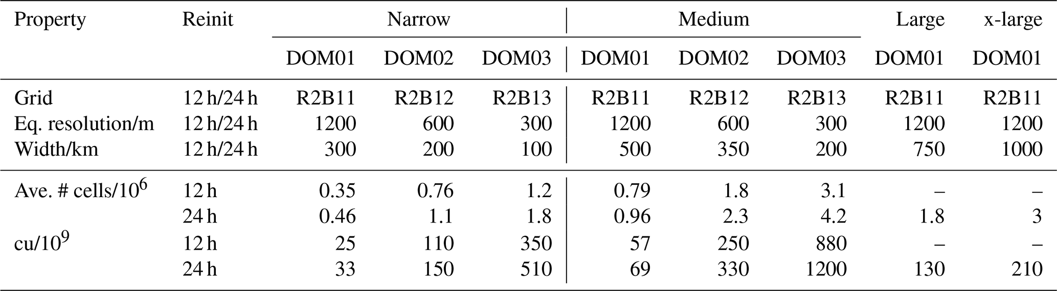
Another important parameter determines the width of the segments across the track, Δs_width. Ideally, the width would be chosen so that the hurricane development would not be significantly influenced by the lateral domain boundaries. In practice, computational constraints are significant, so responsible scientists must select the smallest feasible domain size. Given these two requirements, it is difficult to provide definite advice and determine in advance what the optimum width would be. Two possible configurations are provided in Fig. 6. First, the innermost high-resolution nest at R2B13 is selected so that the across-track width, measured as distance between the track center and the domain edge, is 100 km. Second, a wider setup was tested in which the inner nest was extended to 200 km. Table 1 shows the extent of the two outer high-resolution nests in detail.

Table 1 Comparison of grid and compute requirement parameters across re-initialization configurations and domains (DOM) listed in the different columns. The computational units (cu) refer to the product of the number of time steps and the number of horizontal grid cells and is a measure of the size of a limited area experiment.

High-resolution ICON simulations were performed in the respective grid segments using the latest available version of ICON (v2025-04-2) (ICON partnership, 2025) at the time of the study. We chose 150 vertical levels (analogous to Heinze et al., 2017; Stevens et al., 2020), extending to an altitude of 34 km. Cloud microphysics and radiation were set up similarly to the base run. However, subgrid-scale turbulence was configured with a three-dimensional Smagorinsky-type mixing scheme and convection parameterization was completely deactivated (following Stevens et al., 2020). To enable a consistent re-initialization of complete cloud microphysics, the ICON source code was modified to incorporate vertical interpolation of all microphysical moments (Senf, 2026d). This means that graupel mixing ratios and ice crystal number concentrations, for example, are available as fields when the high-resolution simulations begin and when they are re-initialized. Consequently, all cloud variables are available without discontinuities and abrupt changes throughout the entire simulation period. These initial fields are made available for all nests simultaneously, enabling a seamless continuation of the simulations when switching from one segment to the next.

Figure 7 shows examples of the results of two high-resolution ICON configurations with different grid segmentation. The narrow-size setup is compared with the medium-size setup, both of which have a 12 h re-initialization period. The position of the simulated hurricane pressure minimum in the high-resolution run remains close to the reference track of the base run. There are no significant differences in minimum position for different simulation resolutions, but same grid configuration. However, as expected, the track of the wider setup deviates more strongly from the reference track. This is plausible because the position of the hurricane center in the wider setup is not as strongly constrained by the forcing at the lateral boundaries. The intensity of the simulated hurricane, as shown by the development of the pressure minimum in Fig. 7b and the maximum 10 m wind speed in Fig. 7c, clearly depends on the resolution. This is evident from the greater spread of the curves (esp. in Fig. 7b), which is as large as that induced by different grid configurations. Better resolved convective activity generates particularly high gustiness of the 10 m wind, which explains the fluctuations on the very short time scales in Fig. 7c. However, a more detailed investigation of the resolution effects and their causes and consequences must be postponed to a follow-up study.

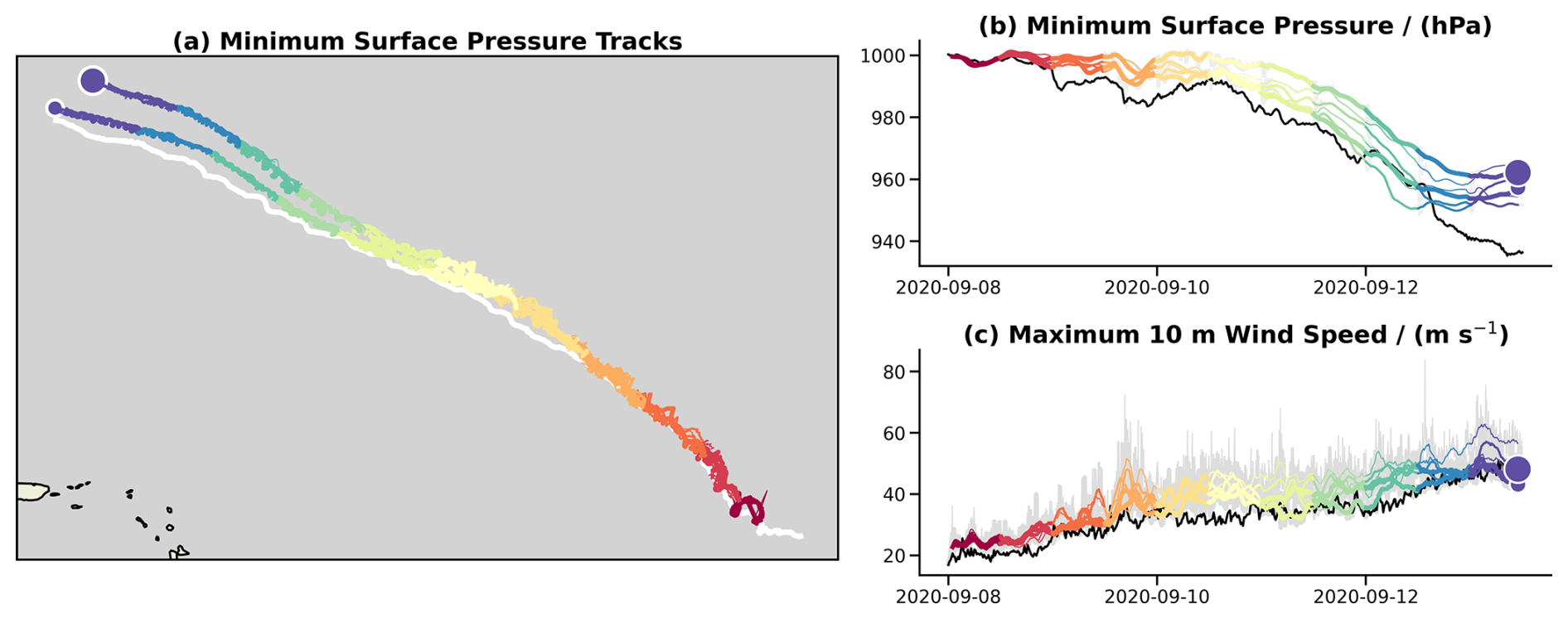
Figure 7 Simulated hurricane characteristics for grid configurations with differently chosen across-track widths. (a) The minimum pressure positions are plotted on a map, with colors representing the respective grid segments. The re-initialization time between successive segments is set to 12 h. The narrow-size setup (small, solid circle at the end of the track) is compared to the medium-size setup (larger, solid circle at the end of the track). Different resolutions are plotted with different line thicknesses, ranging from thick for R2B11 to thin for R2B13, and they partially overlap. Minimum pressure positions from the base run are plotted in white. The minimum pressure and maximum 10 m wind speed are presented using similar color and line encoding as in (a). A running-average filter is applied to the curves in (b), (c) to reduce noise. The original data is shown in light gray shading in the background. Data from the base run is shown in black.

3.4 Prototyping Lagrangian Analysis

The grid remains static during the simulation of a grid segment, and the output is only available for statically defined grids. Output variables are written directly to the ICON grid. Additionally, variables can be internally interpolated in ICON to a regular longitude–latitude grid and then output on this grid. This allows variables to be stored on slightly coarser grids at a higher temporal frequency. Our workflow toolkit includes an option to automatically calculate suitable longitude–latitude grids for the corresponding flexible grid segments. This creates a suitable longitude–latitude grid for each grid segment on which standard analyses can easily be performed. Figure 8 shows an example of such an output, displaying 2 m temperature, 10 m wind speed, reflected solar radiation flux at the top of the atmosphere (TOA), and total column water vapor for a given point in time. The sequence shows three nested grids for each variable, with grid spacings of 1200, 600, and 300 m. The utilization of these representations facilitates the comparison of the effects of varying resolutions on the fine structure of the simulated hurricane. However, Fig. 8 also demonstrates that important parts of the hurricane may no longer be contained within the chosen domains, especially for the finest nest of 300 m grid spacing and rather long integration times of nearly five days. This illustrates the trade-offs responsible scientists must navigate between accuracy, resource requirements, and efficiency.

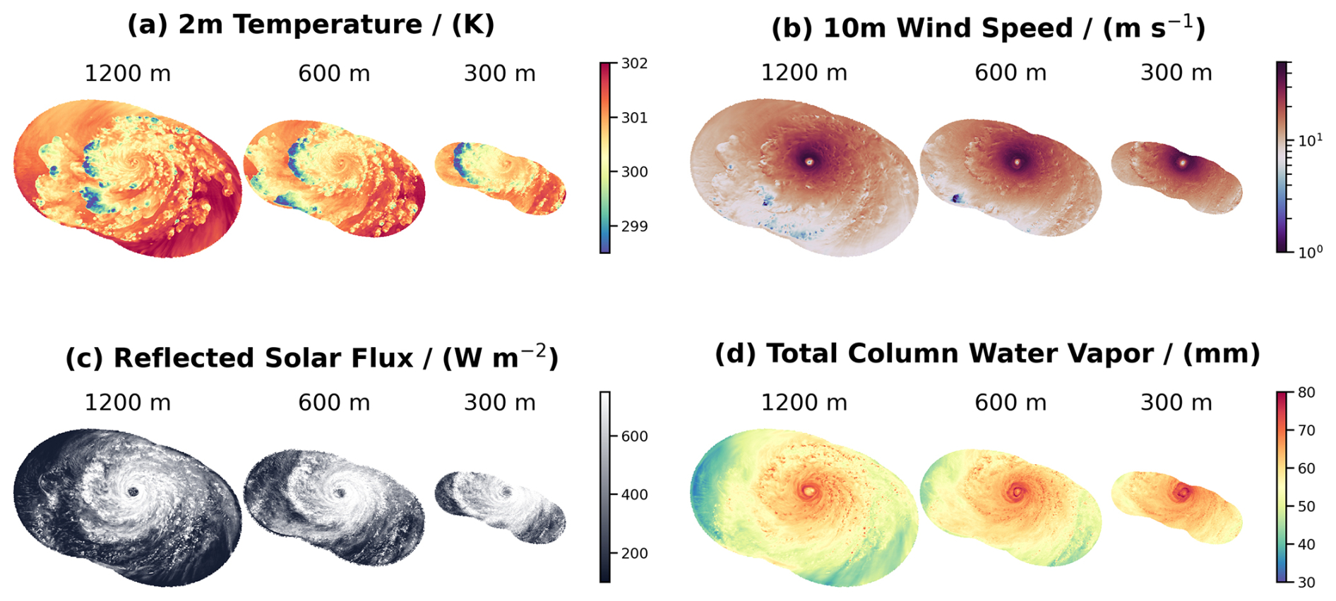
Figure 8 An overview of various variables, shown in the respective nests for a specific grid segment. The grid configuration was chosen so that the re-initialization time is 12 h and the nests have an across-track width of 300, 200, and 100 km, respectively (narrow-size setup). The equivalent grid spacing is indicated above the respective nest. Variables shown are (a) 2 m temperature, (b) 10 m wind speed, (c) reflected solar radiation flux at TOA and (d) total column water vapor for segment 11 at 18:00 UTC on 12 September 2020.

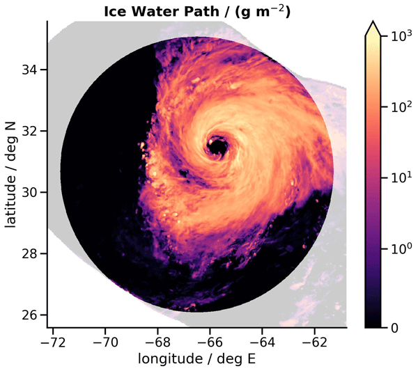
The visualizations on the static grid above have the typical characteristics of an Eulerian analysis, in which the reference points do not change over time. However, our hurricane-centric simulations make it possible to change the perspective by defining only the circle that moves over the reference track as the analysis area (see segment concept in Sect. 2.2). This transformation into a Lagrangian reference system results in a smooth and consistent composition of the hurricane development despite the inherent discontinuity because of the separate grid segments. For example, the evolution of ice water path (IWP) is shown in Fig. 9. Most of the ice produced is located northeast of the hurricane center. The Lagrangian analysis region is highlighted in color. The remaining parts of the segment, which are not used here, are shown in light colors. Interestingly, the Lagrangian approach results in a continuous and smooth path of the IWP. It gives the impression that the grid segments are sliding across the Lagrangian analysis area. Thus, data from different segments can be assembled to create a hurricane-centric analysis that consistently covers several days of hurricane development on a hectometer scale.

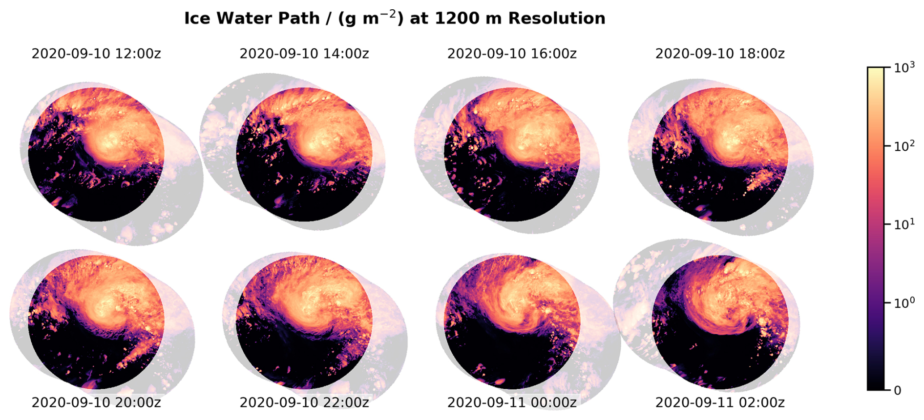
Figure 9 Ice water path is shown as a sequence in a Lagrangian framework. The boldly shaded areas highlight the circular Lagrangian analysis region that follows the track of the reference hurricane. The remaining parts of the respective grid segments are indicated by very light colors. Two-hour steps are made in the temporal sequence. Transitions between segments are visible between the first and second images, as well as between the second-to-last and last images, appearing as shifts in the domain boundaries. Within the Lagrangian analysis region, however, the ice water path evolves smoothly and continuously. Here, the medium-size grid configuration was chosen so that the shown nest (DOM01, 1.2 km grid spacing) has 500 km across-track width with re-initialization time of 12 h.

3.5 Performance and Shortcomings

The following discussion will cover the advantages and disadvantages of the method described so far. One significant advantage is that the target areas of the simulations are relatively small compared to the total region affected by the hurricane. This means that an acceptable number of calculation steps is being performed. Table 2 summarizes computational units (cu) as a measure of computational effort. Here, one cu refers to 1000 time steps of fast physics (dynamical core is sub-stepped by a factor of 5), which are used to integrate one million horizontal grid cells forward. For the narrow-size case, cu increases from 480–700 when transitioning from the 12 h-reinit setup to the 24 h-reinit setup, which corresponds to an increase of approximately 45 %. For the medium-size case, 1190 and 1610 cu are required respectively, representing a factor of between 2.3 and 2.4 more resources than the narrow-size case, showing an increase of 35 % between 12 h-reinit and 24 h-reinit just because of the larger domain size of the 24 h-reinit segments. Therefore, the 12 h-reinit setup is significantly more favorable in terms of resource requirements, and doubling the width of the setup also leads to approximately a doubling of resource requirements. The costs for expanding the setup to large and extra-large sizes are also shown. However, when comparing the numbers, it should be noted that only the outermost nest with a grid spacing of 1.2 km was considered for the larger setups and that the complete setup consisting of three respectively refined nests requires 20–25 times more resources.

To assess how the savings of our method compare to classic regional, limited-area applications, two reference configurations are introduced in Table 2. The first is a tube-like setup that extends over the full hurricane track over the entire simulation period without splitting it into shorter segments. Such a tube shares the same cross-track geometry and nesting structure as our hurricane-centric segments, but is integrated as a single contiguous domain without re-initialization. The resource requirements for the tube, listed under the “6 d” re-initialization interval, amount to approximately 2640 and 5440 cu for the narrow and medium three-nest configurations and 320 and 470 cu for the single-domain large and x-large setups, respectively. The second reference, labeled “classic” in Table 2, represents a conventional fixed limited-area domain and is constructed as the smallest regular longitude–latitude bounding box that fully encloses the tube geometry for the respective cross-track width. For the single-domain case at 1.2 km grid spacing, the classic limited-area approach amounts to approximately 800 cu; a three-nest configuration requires around 20 000 cu. Compared to this classic reference, the tube configurations already yield notable speedup factors of 7.6, 3.7, 2.5, and 1.7 for the narrow, medium, large, and x-large setups, respectively. Dividing the tube into short, frequently re-initialized segments adds a further factor of approximately 2–6, depending on the chosen across-track width and re-initialization interval. Together, the segment configurations with frequent re-initialization achieve the largest speedups: factors of up to 42 and 17 for the narrow and medium three-nest setups with 12 h re-initialization intervals, and up to 6.2 and 3.8 for the single-domain large and x-large setups with 24 h re-initialization intervals (see Table 2). Considering the risk of model errors or suboptimal settings requiring reruns of high-resolution simulations, the use of our flexible workflow appears well justified.

Table 2 Comparison of compute requirement and compute cost parameters across re-initialization configurations and domain sizes. The reinit row “6 d” indicates a nested tube configurations with effectively no re-initialisations. The term “classic” refers to a potential, fixed domain configuration such that a corresponding tube configuration could be accommodated. Single domain configurations are marked by ^*, all other domain configurations consist of three online coupled nests. The computational units (cu) refer to the product of physics timesteps and number of horizontal grid cells. The number of nodes and node hours refers to DKRZ Levante nodes with 128 cores for the 12 h-reinit setup and to JSC JUWELS nodes with 48 cores for the 24 h-reinit setup.

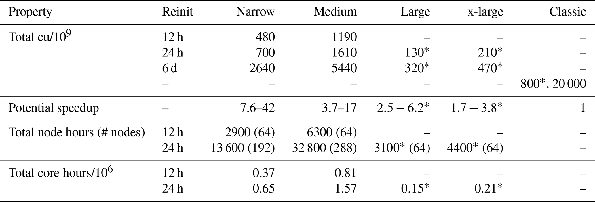
In addition to the hypothetical requirements, Table 2 also shows the actual costs of executing the respective setups. The 12 h-reinit setup was calculated on the DKRZ Levante platform using an ICON build created with the Intel compiler without the thread-based parallelization via OpenMP. Production runs were performed on 64 nodes, generating costs of 2900 and 6300 node-hours for the narrow- and medium-size cases, respectively. This increase in costs by a factor of 2.2 roughly corresponds to the calculated increase in demand. The 24 h reinit setup was calculated on the JSC JUWELS platform, which has fewer computing units than Levante, with 48 cores per node compared to 128. An ICON build was created and used on JUWELS with GCC, as well as without OpenMP. The narrow-size setup was calculated on JUWELS with 192 nodes, generating costs of 13 600 node-hours. The medium-size setup was calculated with 288 nodes and generated costs of 32800 node-hours. Comparing the core hours values between Levante and JUWELS reveals that execution on JUWELS is 20 %–40 % less efficient. This difference is probably due to the different compilers and their respective optimization settings, rather than hardware differences.

The immense increases in efficiency of our hurricane-centric setup however come at a price. Due to the limited size of the regional setups, the hurricane under consideration cannot develop completely freely and always remains influenced by the forcing at the lateral boundaries, which is stronger for a more narrow setup. In addition, the re-initialization procedure during the transition between segments introduces further challenges. The mix of ICs detailed in Sect. 2.3, which consist of different data sources inside and outside the overlap region of two subsequent segments, creates a discontinuity. This is smoothed out in the transition using a distance-weighted average. Despite this, the merged ICs can excite spurious sound and gravity waves, and re-initialization effects occur at the beginning of a simulation in a new segment. The following section evaluates the impact of these effects on simulation quality.

3.6 Analysis of Re-initialization Effects

To investigate the re-initialization behavior in a controlled manner, we conducted sensitivity experiments following the same grid configurations as listed in Table 1, but with the runtime of each segment extended by three hours. This creates a three-hour temporal overlap between consecutive segments, enabling a direct comparison of the atmospheric state from two successive segments at the same point in time and thus providing a pathway for directly quantifying re-initialization effects. To keep the analysis tractable, all sensitivity experiments were performed exclusively for the outermost nest (DOM01) at 1.2 km grid spacing. In addition, two parameter settings are compared throughout: the production setting with init_latbc_from_fg=.FALSE. (labeled “LBC flag OFF”) and an updated setting with init_latbc_from_fg=.TRUE. (labeled “LBC flag ON”). The latter has been recommended by the ICON community since early 2026 to reduce model biases arising from mismatches between the initial lateral boundary conditions and the initial model state (see ICON Documentation, 2026).

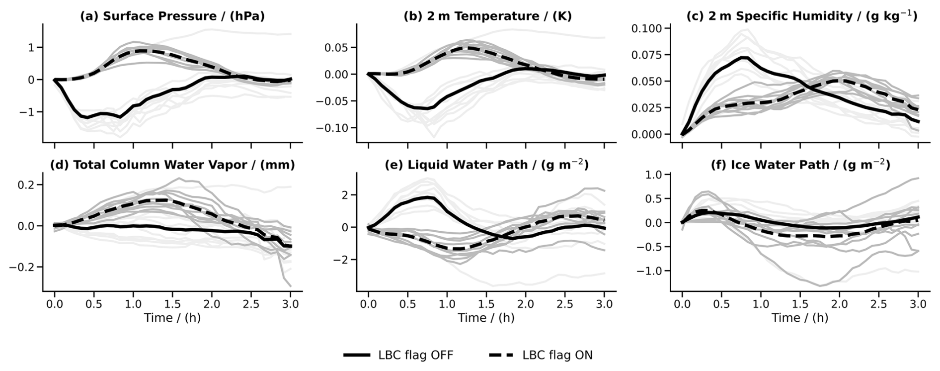
Figure 10 Temporal evolution of median values of surface and integrated cloud variables evaluated in the circular Lagrangian analysis region. The curves show the instantaneous difference between values from segment k and the corresponding values from segment k−1 extended by 3 h, for (a) surface pressure, (b) 2 m temperature, (c) 2 m specific humidity, (d) total column water vapor, (e) liquid water path, and (f) ice water path. Results are shown for the medium setup with 12 h-reinit. Gray curves show the evolution for individual segments, while the thick black curve shows the mean across all segments. Two parameter settings are compared: the experiment with the LBC flag deactivated ((init_latbc_from_fg=.FALSE.), thin light gray and solid black lines) and the experiment with the LBC flag activated ((init_latbc_from_fg=.TRUE.), thin gray and dashed black lines).

In the following, we analyze the time series of thermodynamic and water-related atmospheric parameters for the first three hours in Fig. 10. There, the median values in the circular Lagrangian analysis regions (see Sect. 3.4) of selected surface and cloud variables are presented. For each variable, the instantaneous difference between segment k and the corresponding values from segment k−1 extended by 3 h is shown, allowing a direct quantification of re-initialization-induced deviations between consecutive segments. The figure was created for the medium-size, 12 h-reinit DOM01 setup with 1.2 km grid spacing (see Table 1). Light gray curves show the individual segment differences, and the thick solid (dashed) black curve gives their mean for the LBC flag OFF (ON) setting. The surface pressure in Fig. 10a shows a negative anomaly with peak values around −1.2 hPa after about 30 min of integration time for the LBC flag OFF setting. An opposing positive but slightly weaker anomaly of around 0.9 hPa is visible for the LBC flag ON setting, with the peak shifted to around 70 min. Both differences appear to have converged after approximately 2 h, by which point they have decayed to near-zero values. The 2 m temperature curve in Fig. 10b also shows a systematic negative peak of around −0.06 K at 30 min for LBC flag OFF, and a positive peak of around 0.05 K at 75 min for LBC flag ON. Temperature differences likewise vanish after approximately 2 h. The curves for 2 m specific humidity show positive differences for both LBC flag settings, with peak values of 0.07 g kg⁻¹ at 45 min for LBC flag OFF and 0.05 g kg⁻¹ at 120 min for LBC flag ON. The specific humidity difference for the LBC flag ON setting converges more slowly than for LBC flag OFF, with near-zero values not yet reached by 3 h. The individual curves for total column water vapor (TCWV), liquid and ice water path (LWP, IWP) in Figs. 10d–f show considerable variability over the three-hour window. The LBC flag ON setting tends to produce slightly larger mean peak values for TCWV and IWP, and smaller ones for LWP, and its peak consistently occurs later than for LBC flag OFF. Overall, the LBC flag ON setting tends to produce smaller peak differences for surface pressure and near-surface temperature, suggesting it may be the preferable choice for future applications, though its re-initialization effects appear to persist somewhat longer legitimating our choice of the LBC flag OFF setting for the production runs in this study.

Figure 11 provides a comprehensive statistical comparison of re-initialization effects across different configurations. As in Fig. 10, the analysis evaluates percentiles from segment k, here taken 30 min after initialization, and segment k−1 extended correspondingly. Nine percentiles (10 %–90 % in 10 % steps) of each field are computed across the Lagrangian analysis region separately, and their differences are taken. These per-segment differences are visualized as stacked histograms, with color coding by segment to enable direct comparison between setups.

The statistical results reveal distinct patterns for different atmospheric variables. Re-initialization effects are particularly visible when the values in the distributions significantly deviate from zero. For surface pressure, this pattern is clearly evident in Fig. 11a and e for the narrow setup. Surface pressure values scatter between −1 and −2 hPa. Comparing the effects of re-initialization time shows that longer intervals lead to slightly larger re-initialization effects in surface pressure (comparing Fig. 11a and e for narrow setup and Fig. 11i and m for medium setup). Domain size also influences these effects: larger domains (Fig. 11q and u) show considerably less deviation from zero at 30 min, indicating that systematic re-initialization effects are less pronounced for larger domains. For temperature, similar effects are clearly visible. The value appear to be distributed to slightly lower magnitudes for the 12 h-reinit setup than for the 24 h-reinit setup. For large and x-large setups, temperature anomalies scatter around zero for all segments. Cloud variables such as LWP and IWP show significant spread in the narrow setup (Fig. 11c,d,g and h). As domain size increases, this variability decreases, likely due to more robust spatial statistics. The considerable variability in cloud variables masks potential re-initialization effects. Overall, while our hurricane-centric workflow introduces uncertainties through re-initialization effects, these remain sufficiently small and are outweighed by the substantial efficiency gains achieved.

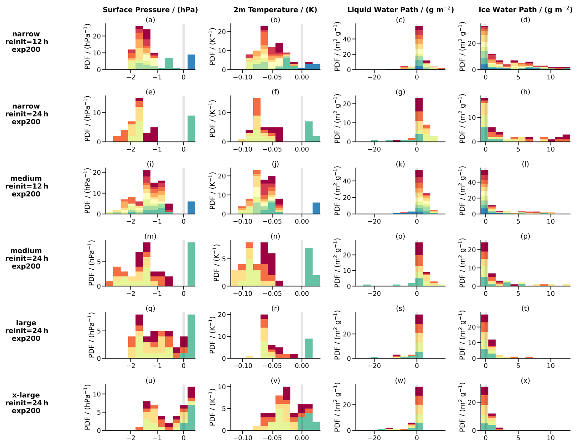
Figure 11 Statistical summary of potential re-initialization effects plotted as colored bars stacked on top of each other for each segment. The color coding is the same as in Fig. 6. At 30 min after initialization of segment k, nine percentiles (10 %–90 % in 10 % steps) of each field are computed across the Lagrangian analysis region separately for segment k and segment k−1 extended by 3 h, and their pairwise differences are taken. These per-segment differences are statistically summarized as probability density functions. The six rows show the respective setups, with the narrow and medium setups shown for re-initialization periods of 12 and 24 h, respectively. The columns show surface pressure, 2 m temperature, liquid water path, and ice water path. The re-initialization analyses are only shown for the outer nest with a grid spacing of approximately 1 km.

4 Conclusions

This study presents a flexible workflow for the atmospheric model ICON that enables efficient high-resolution simulations in a hurricane-centric reference framework through a segment-based grid and pre-processing approach. The methodology demonstrates the general feasibility of conducting hectometer-resolution simulations of large, organized atmospheric phenomena like hurricanes in the tropics. Instead of investing in fixed and spatially extended regional domains throughout the entire simulation period, our flexible method follows the motion of a hurricane and generates tailored grid segments.

The technical implementation successfully automates key components of the workflow, including hurricane tracking, flexible grid generation, and initial condition preparation and merging across consecutive segments. The segment concept, which divides hurricane tracks into overlapping temporal windows of 12–24 h, provides a practical framework for efficient utilization of computational resources. The workflow toolkit demonstrates portability across different HPC platforms, having been successfully deployed on both DKRZ Levante and JSC JUWELS systems with appropriate platform-specific configurations.

The application of the workflow is demonstrated for Hurricane Paulette (2020). High-resolution simulations with grid spacings down to 300 m were performed using different segment configurations. Variations in re-initialization intervals of 12 and 24 h are explored that determine the respective along-track lengths of the segments. Additionally, different overall domain sizes are investigated by varying the across-track widths with tested configurations being rather narrow, medium-sized, large and extra large. The results indicate that the hurricane track remains consistent with the base run and mainly depend on the across-track size of the chosen configuration, while intensity metrics such as minimum pressure and maximum wind speed exhibit sensitivity to resolution in our multi-nested setups. A Lagrangian framework enables a hurricane-centric view, facilitating continuous analysis of variables like liquid and ice water path across the segmented simulations.

The increase in computational efficiency is substantial compared to traditional fixed-domain approaches. A track-following tube geometry alone reduces resource requirements by factors of 1.7–7.6 relative to an appropriately chosen longitude–latitude bounding box around the hurricane. Segmenting the tube into short, frequently re-initialized intervals adds a further factor of 2–6, yielding total speedups of up to 42 for the narrowest three-nest configuration. The setup with 12 h re-initialization intervals proves to be more efficient than 24 h intervals, requiring 35 %–45 % fewer computational resources while maintaining comparable simulation quality. Domain size scaling shows predictable resource scaling, with the twice as large medium-width configurations requiring approximately 2.3 times the resources of narrow configurations. However, the approach has notable limitations when the across-track width is set too narrowly, the domain may fail to encompass the entire phenomenon, a shortcoming that becomes especially evident for our narrow-size configurations. The analysis of re-initialization effects reveals systematic but manageable impacts during segment transitions, with surface pressure showing negative anomalies on the order of 1 hPa that decay within 2 h after re-initialization. The re-initialization effects are more pronounced in narrower domain configurations but remain sufficiently small to justify the substantial computational efficiency gains achieved by the hurricane-centric approach.

Several promising directions for methodological enhancement emerge from this work. On the technical side, extending the workflow to support more than three nesting levels would provide greater refinement flexibility and enable even finer resolution simulations. Similarly, offering greater flexibility in selecting the grid from which the refinement cycle is initiated (currently the grid of the base run) would allow for more diverse and independent nesting hierarchies. A further interesting area for development lies in improving the re-initialization procedure itself. Currently, the distance-weighted blending approach, while effective, could potentially be enhanced by integrating techniques from data assimilation, such as the Incremental Analysis Update (IAU) method available in the numerical weather prediction configuration of the ICON model. This approach might have the potential to substantially reduce spurious artifacts arising from the merging of initial conditions between consecutive segments. Additionally, future work could also investigate how the method performs over land, where re-initialization of subgrid-scale heterogeneities in land surface properties can be challenging and may introduce additional difficulties. Importantly, all such technical improvements must maintain spatial and structural consistency of simulated core variables across segment transitions such that Lagrangian analyses remain continuous and meaningful.

Beyond technical refinements, the computational efficiency gains achieved here enable new scientific applications. The method now makes high-resolution hectometer-scale simulations of additional hurricanes computationally feasible, opening opportunities for detailed dynamical analysis and process studies of a broader range of tropical storms. The reduced computational cost further enables simulation ensembles to be conducted in scientific studies, providing higher confidence in identifying systematic effects. Particularly noteworthy is the potential for perturbed parameter ensembles that would deepen our understanding of how model parameterizations influence the representation of convective organization, eyewall structure, and other small-scale phenomena in tropical cyclones. These applications demonstrate how advances in efficient simulation frameworks can open new avenues for investigating the cloud physics and dynamics of extreme atmospheric phenomena.