Effects of assimilating phytoplankton carbon in marine ecosystem modelling in NEMO4.0.4-MEDUSA2.0-PDAF2.0

The state of the marine ecosystem can be estimated by a combination of numerical models and satellite observations through data assimilation (DA) methods. Satellite data representing phytoplankton chlorophyll are typically used in operational marine ecosystem prediction. These data are derived from ocean colour measured by optical satellite observations. Recently a new phytoplankton carbon product, from the ESA funded BICEP project made available from the UK CEDA Archive, has been derived through a novel processing of ocean colour. This novel carbon product captures aspects of phytoplankton biomass composition that chlorophyll alone does not represent. Here, we investigate the effects of assimilating the new carbon product on the modelling of the marine ecosystem. The investigation is carried out in a newly developed global ensemble DA system for the marine ecosystem using a coupled ocean-biogeochemistry model, NEMO-MEDUSA, and the Parallel Data Assimilation Framework. With the ensemble DA system, the evaluation can take the time-dependent uncertainty of the marine ecosystem and the reliability of the ensemble into account. We demonstrate that, compared with assimilating only the chlorophyll product, which may degrade the seasonality of phytoplankton carbon, assimilating the new carbon product can provide different patterns of adjustment and seasonal anomalies in phytoplankton concentrations, surface pCO₂, and oxygen. Our findings reveal that simultaneously assimilating both phytoplankton chlorophyll and carbon products in a complex marine ecosystem yields more balanced estimates of phytoplankton biomass than assimilating a single phytoplankton product.

1 Introduction

The marine ecosystem mediates the global carbon and oxygen budgets and supports human activities (Wanninkhof et al., 2013). In particular, as the base of the food web, phytoplankton sequestrate carbon and emit oxygen, accounting for 50 % of total global net primary production estimated on the order of 50 Gt C yr⁻¹ (Falkowski, 1994; Buitenhuis et al., 2013; Johnson and Bif, 2021; Ryan-Keogh et al., 2023). Studies have shown the need for reliable forecasting and reanalysis data for the monitoring and management of the health of marine ecosystems and fisheries (Lehodey et al., 2008; Berx et al., 2011; Fennel et al., 2019).

Existing operational forecasting and reanalysis products adopt data assimilation (DA) methods to combine marine ecosystem models with observations. Observations are used by DA to optimise the model parameters (e.g., Hemmings et al., 2015; Schartau et al., 2017) and estimate the state of the marine ecosystem models (e.g., Ford et al., 2012; Gehlen et al., 2015; Ford and Barciela, 2017; Pradhan et al., 2020). Thanks to the good spatio-temporal coverage of the satellite observations, DA applications focus on assimilating total phytoplankton chlorophyll-a products derived from satellite ocean colour for their use as proxies for phytoplankton biomass in ocean ecosystem modelling (Gregg, 2008; Ford et al., 2012; Simon et al., 2015). Note that, for brevity, chlorophyll-a and chlorophyll are used interchangeably in this study.

One limitation of satellite ocean colour is its inability to differentiate the vertical structure of the euphotic zone near the ocean surface (Arteaga et al., 2022). This issue can be mitigated by the deployment of new in-situ observations using autonomous instruments such as floats in the Biogeochemical-Argo program (Verdy and Mazloff, 2017; Ford, 2021) and gliders (Skákala et al., 2021). These in-situ observations not only observe the subsurface chlorophyll but also other key state variables of the marine ecosystem, such as the oxygen and nutrients that cannot be observed by satellite. However, besides its limited spatial and temporal coverage, operational assimilation of BGC-Argo floats can still face other technical challenges. For example, the chlorophyll estimates from BGC-Argo floats can be biased because they are estimated from measurements of fluorescence (Roesler et al., 2017). These biases are not addressed in studies assimilating BGC-Argo floats, e.g., in synthetic experiments performed by Ford (2021). This suggests the need for further research on bias correction for BGC-Argo floats in DA systems. In addition, research also suggested discrepancies between observations from satellites and BGC-Argo floats (Baudena et al., 2025). Such discrepancies pose additional challenges for joint assimilation of satellite and BGC-Argo data. Hence, satellite ocean colour is still a vital resource, especially on a global scale.

Assimilating satellite phytoplankton chlorophyll products (referred to as chlorophyll hereafter) can effectively control errors in modelled chlorophyll. However, even though the chlorophyll provides a proxy for biomass, assimilating chlorophyll does not necessarily correct other compositions of phytoplankton such as silicate, nitrogen and carbon, or factors that constrain chlorophyll such as the availability of light, nutrients, and species composition. For example, if the model simulations overestimate the phytoplankton biomass, reducing the chlorophyll by DA does not directly change phytoplankton carbon or nitrogen concentrations. Hence, operational marine biogeochemical DA requires balancing schemes, which distribute DA increments of chlorophyll to other model variables for a consistent model state across variables, e.g., different phytoplankton compositions and nutrients, after the DA update (Hemmings et al., 2008), or rely on estimates of error covariances from an ensemble of model forecasts (Pradhan et al., 2020). Yet, as discussed by Skákala et al. (2024), phytoplankton community compositions are the most uncertain and least observable variables in the marine ecosystem even when a balancing scheme is applied. An additional challenge is that phytoplankton are typically represented in models by a number of functional types (PFTs), such as different sizes of chlorophyll and nitrogen. This means that either PFT products need to be derived from the ocean colour data prior to assimilation or the increments of total chlorophyll need to be split during assimilation. Recent efforts were made to derive PFTs from satellite data with uncertainty validations (see e.g., Xi et al., 2021). These products for PFTs led to studies showing improvements from assimilating PFTs instead of total chlorophyll data (Ciavatta et al., 2018; Skákala et al., 2018; Pradhan et al., 2020), as inferring PFTs from chlorophyll errors using only balancing schemes is challenging. Alternatively, Pradhan et al. (2020) showed improvements in updating multiple PFTs through the use of ensemble error covariances when only total chlorophyll was assimilated. However, this is not as desirable as directly assimilating PFT products. Nevertheless, due to the various definitions of PFTs in different models, universal PFT products are not yet available.

Besides chlorophyll data, other phytoplankton products, such as particulate inorganic ocean carbon and particulate organic ocean carbon, can be derived from satellite ocean colour (Siegel et al., 2005; Yang et al., 2024) independently of chlorophyll in their derivation. In particular, satellite ocean colour can be used to derive phytoplankton carbon (Behrenfeld et al., 2005; Graff et al., 2015; Bellacicco et al., 2020) using an empirical relationship between the backscattering of particles and phytoplankton carbon supported by both direct (Graff et al., 2015) and indirect evidence based on the ratio between chlorophyll and carbon and based on nutrient stress from light (Bourdin et al., 2026; Martiny et al., 2026). These products are used to understand the ocean's biological pump and carbon cycles in addition to the chlorophyll products (Siegel et al., 2023; Bourdin et al., 2026). Recently, in the ESA Biological Pump and Carbon Export Processes (BICEP) project, a new phytoplankton carbon (referred to as carbon hereafter) product has been derived from the ocean colour observations (Sathyendranath et al., 2021b). The product is derived using an approach different from the backscattering of particles used in other carbon products. The new product is based on the chlorophyll-to-carbon ratio from a photoacclimation model where the ratio varies with the photosynthetically active radiation available in the ocean mixed layer. Compared to other carbon products with limited quality assessments (e.g., NASA Ocean Biology Processing Group, 2025), the product's chlorophyll-to-carbon ratio is validated with field data (Sathyendranath et al., 2020).

In this study, we explore the effects of assimilating the newly derived carbon product so that we can understand whether assimilating phytoplankton carbon can provide additional information compared with assimilating the chlorophyll product alone in the modelling system. Note that, here, as this study focuses on assessing the modelling response of assimilating carbon products, we do not seek the best carbon product for DA, and opt to use the validated off-the-shelf observational dataset. To our knowledge, whilst there are studies assimilating particulate organic carbon (POC, Kettle, 2009; Xiao and Friedrichs, 2014), phytoplankton carbon assimilation is not well-studied in the literature. This new observation product allows us to investigate direct DA adjustments to carbon without the balancing scheme. Besides phytoplankton variables, we further investigate the impact of the assimilation on other model variables in a marine ecosystem model, such as zooplankton, pCO₂, and oxygen. These evaluations enable us to assess the potential benefits of assimilating the new ocean colour product and its impact in comparison with the widely assimilated total chlorophyll data. To perform such an evaluation, we adopt the coupled ocean-biogeochemistry model, NEMO-MEDUSA (Madec et al., 2023; Yool et al., 2013). Ford (2021) has applied NEMOVAR, a 3DVar system, to the global coupled NEMO-MEDUSA. In order to incorporate new model variables into the 3DVar system one would need an estimation of forecast errors. These are typically estimated by sophisticated background error covariance modelling accounting for the correlation scales and balancing conditions of the forecast errors. Without these efforts for the background error covariance, a 3DVar system cannot be used with the new product. To overcome this issue, instead of using the existing NEMOVAR setup, we develop an ensemble DA system using the Parallel Data Assimilation Framework (PDAF, Nerger and Hiller, 2013). In this ensemble DA system, the forecast errors can be estimated by an ensemble of forecasts. Moreover, compared to NEMOVAR, where the background error covariance matrix does not change with time, the ensemble DA system can provide a time-dependent forecast error covariance matrix accounting for the temporal change of error dynamics.

In Sect. 2, we provide a description of the full ensemble DA system, comprised of the coupled ocean-biogeochemistry model, the assimilated observations, and independent in-situ observations for assessment. In Sect. 3, the processing of the state vector and observations used in this study are described. In Sect. 4, a suite of experiment setups used for assessing the effects of assimilating the carbon product are described. We evaluate the statistical skill of the analysis and the impact of the DA on the modelled marine ecosystem and pCO₂ and oxygen in Sect. 5. In Sect. 6, we discuss the benefits of assimilating additional satellite ocean colour products and the future developments of the ensemble DA system.

2 Data assimilation system

To investigate the impact of assimilating the newly derived carbon product on the modelling of the marine ecosystem, we develop a new global ensemble ocean-biogeochemistry DA system employing the Parallel Data Assimilation Framework (PDAF, Nerger and Hiller, 2013), as detailed in Fig. 1.

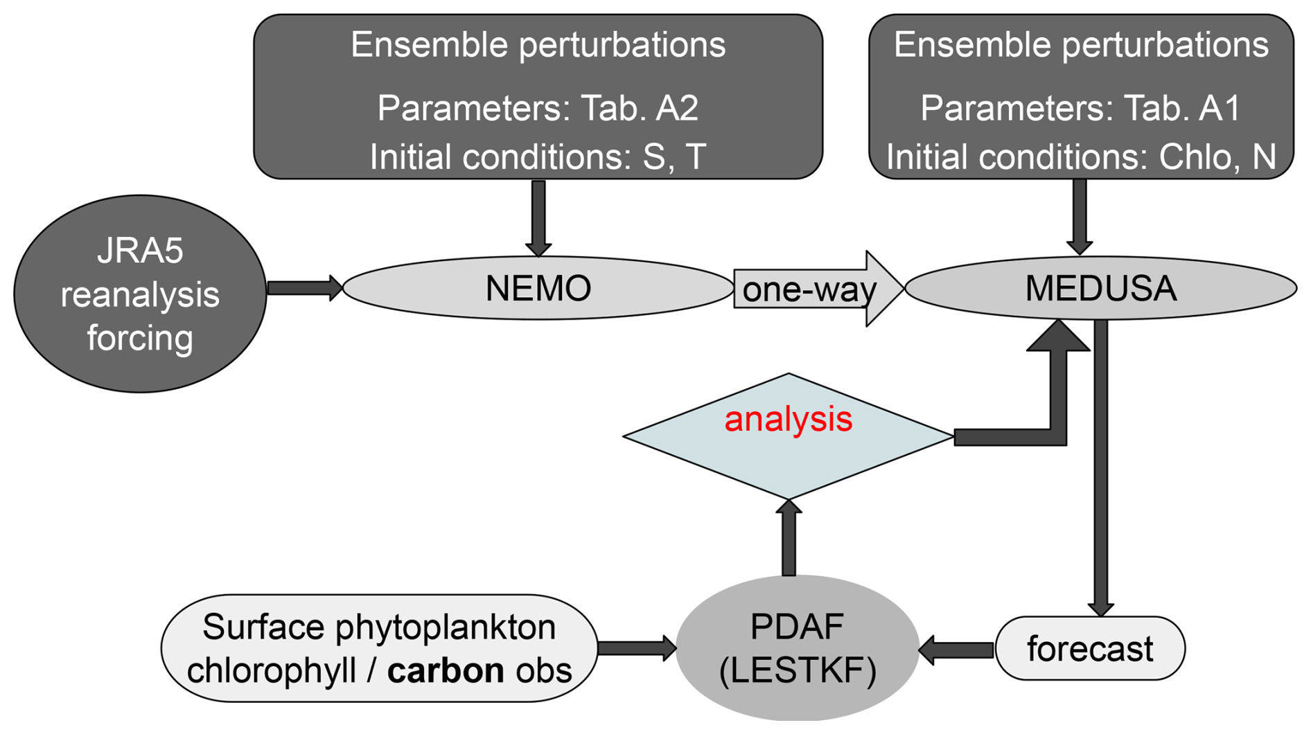
Figure 1 An illustration of the data assimilation system where an ensemble of forecasts is obtained from the one-way coupled NEMO-MEDUSA forced by the JRA-55 reanalysis whereas the satellite surface chlorophyll and carbon observations are assimilated. The analysis (reconstructed state) is used to initialise the following ensemble forecast. Perturbed parameters are listed in the Appendix in Table A2 for MEDUSA and Table A1 for NEMO. Here, Parallel Data Assimilation Framework (PDAF) is the computational framework and local error subspace transform Kalman filter (LESTKF) is the DA algorithm provided by PDAF.

2.1 NEMO-MEDUSA-PDAF

The physical ocean model is the Nucleus for European Modelling of the Ocean (NEMO) version 4.0.4, which solves the primitive equations of the ocean (Madec et al., 2023). The model is configured on a 1° tripolar global extended ORCA grid with 75 vertical z^*-coordinate levels. The model surface is forced by atmospheric wind, air temperature, dew point temperature, humidity, precipitation, sea level pressure, snowfall rate, and long- and short-wave radiation provided by the JRA-55 reanalysis product (Kobayashi et al., 2015).

The marine ecosystem model coupled to NEMO is the Model of Ecosystem Dynamics, nutrient Utilisation, Sequestration and Acidification (MEDUSA), an intermediate complexity model (Yool et al., 2013). Although marine biogeochemical processes can have a strong impact on physics (Manizza et al., 2005; Skákala et al., 2022), the models in current DA systems are still primarily one-way coupled (Gehlen et al., 2015; Yumruktepe et al., 2022; Polton et al., 2023). Hence, even though two-way coupling can provide a better feedback between the ocean and biogeochemistry, following the common practice of using one-way coupled model avoids the need to investigate the impact of two-way coupling, which is outside the scope of this work. Hence, the coupling to NEMO is one-way; that is, the marine ecosystem model is forced by the physical ocean, but has no feedback from the ecosystem to the physics.

The model includes nutrients, phytoplankton, zooplankton and detritus to simulate marine nitrogen, silicon, iron, alkalinity and oxygen cycles with a benthic ecosystem for seafloor organic pools. In the model, the evolution of phytoplankton concentration is primarily represented in terms of nitrogen biomass. These features allow MEDUSA to simulate complex marine ecosystem processes relevant in climate models. Beyond these components, MEDUSA is capable of simulating the CO₂ uptake of marine ecosystems. The carbon cycle simulation is enabled by the pCO₂, pH, alkalinity, and by carbonate species like H₂CO₃, HCO${}_{\mathrm{3}}^{-}$ and CO${}_{\mathrm{3}}^{\mathrm{2}-}$.

In MEDUSA, the phytoplankton biomass is represented by nitrogen. The phytoplankton chlorophyll is also explicitly modelled as a prognostic variable, influenced by the primary production of the phytoplankton biomass. Phytoplankton chlorophyll in turn act as the light limit of the primary production in MEDUSA. Phytoplankton biomass in MEDUSA is divided into diatom and non-diatom PFTs. The diatom phytoplankton variable is responsible for silicon uptake and biogenic silica production and the non-diatom phytoplankton variable represents the non-silicifying phytoplankton community. Hence, diatom phytoplankton silicate is also explicitly modelled besides nitrogen and chlorophyll. MEDUSA models diatom phytoplankton as “large phytoplankton” based on the fact that diatoms are a key component of large phytoplankton even though diatom phytoplankton span a large range of sizes (Yool et al., 2011). This is motivated by the fact that zooplankton graze phytoplankton according to their sizes as zooplankton are divided into microscopic and mesoscopic size classes. As a simplification of the real ecosystem, these functional types do not capture the full diversity of plankton trophic strategies, e.g., mixotrophy, but they remain a useful approximation of the broader plankton ecosystem. For consistency with the observations the nitrogen fields in this study are represented as carbon, with the conversion between carbon and nitrogen following the model assumption of a fixed ratio between C : N of 6.625 : 1. For clarity, we describe nitrogen in terms of its carbon equivalent (hereafter referred to simply as “carbon”).

The data assimilation algorithm is implemented using PDAF, a flexible and efficient framework to enable ensemble data assimilation. The coupling between NEMO and PDAF is adapted based on an open-source NEMO-PDAF coupling available at https://github.com/PDAF/NEMO-PDAF (last access: 13 August 2026). This ensemble DA system provides the flexibility for assimilating not only the ocean physical variables but also arbitrary marine biogeochemical variables. This system also comes with the flexibility to implement a new observation module, which permits the assimilation and comparison of different observation products in this study. The efficient NEMO-PDAF implementation allows for in-memory exchange of data between the model and the DA algorithms. As a result, the DA can be performed without interrupting the model simulation. This study adopts the local error subspace transform Kalman filter (LESTKF, Nerger et al., 2012), which is a specific ensemble DA algorithm provided by the computational framework of PDAF. Constructed with the assumption of a Gaussian distribution, the LESTKF approximates the forecast and analysis error distribution by an ensemble of model forecasts. The LESTKF can assimilate sparse and irregularly spaced observations without spatial interpolation of the observation product. In our configuration of the LESTKF, model variables at each grid point assimilate observations adjacent to that point within a radius of 200 km. The DA increment at grid points without observations is computed based on the spatial correlation between the grid point and the observation locations.

2.2 Observations

2.2.1 Assimilated observations

As our goal is to investigate the effects of assimilating the carbon product instead of constructing the best performing DA system, we follow common practices in operational systems (Skákala et al., 2025). In this study, two datasets are assimilated into NEMO-MEDUSA: a new monthly phytoplankton carbon product and a chlorophyll-a dataset for reference. This means that the DA system inherits some challenges in operational DA as we do not assimilate additional observations to improve vertical profiles.

The carbon product is created from the ESA Biological Pump and Carbon Export Processes (BICEP) Project (Sathyendranath et al., 2020, 2021b). The carbon is derived from ocean colour using empirical models and additional datasets (Kulk et al., 2020). Note that the derived carbon product makes use of chlorophyll product suggesting a correlation between these two products. The dataset contains monthly global surface carbon from 1998 to 2020 at a spatial resolution of 9 km, with phytoplankton divided into PFTs of pico-, nano-, and micro-phytoplankton. This size division differs from the PFTs used in MEDUSA, whose phytoplankton are divided into diatom and non-diatom classes. Thus, instead of assimilating individual PFTs, the total surface carbon is assimilated. The analysis is distributed to the model variables by post-processing, as will be discussed in detail in Sect. 3.

As a reference, the commonly used satellite chlorophyll is also assimilated. The assimilated data set is the global chlorophyll-a data product gridded on a geographic projection, Version 5.0 from the ESA Ocean Colour Climate Change Initiative (OC-CCI) project (http://www.esa-oceancolour-cci.org/, last access: 13 August 2026,  Sathyendranath et al., 2021a). The product merges data from satellite sensors of SeaWiFS (Sea-viewing Wide Field-of-view Sensor), MODIS (Moderate Resolution Imaging Spectroradiometer), VIIRS (Visible Infrared Imaging Radiometer Suite), and OLCI (Ocean and Land Colour Instrument), matched to MERIS (Medium Resolution Imaging Spectrometer). The global daily product spans a time period of 1997–2020, and has a spatial resolution of 4 km. Based on validation against in situ observations, this dataset provides an estimate of both observation error and biases. In this study, we assimilate both composite daily and monthly bias-corrected surface chlorophyll products.

Both observation products do not contain information under clouds. Daily products only contain pixels with available observations. The composite monthly product is computed as the monthly average of available daily data excluding missing data. Because the monthly product is based purely on data without clouds, it cannot resolve short term processes (e.g. photoacclimation) under clouds over the course of the month.

2.2.2 Independent assessment observations

To assess the DA system, we use in situ observations of chlorophyll and carbon data. The in situ chlorophyll data are obtained from the BGC-Argo program (Biogeochemical-Argo Planning Group, 2016; Roemmich et al., 2019; Argo, 2000). The BGC-Argo program extends the Argo program, which is an international program that deploys automatic instruments floating with ocean currents. The BGC-Argo floats provide vertical profiles for both physical variables such as temperature, salinity, and pressure, and biogeochemical variables. In this study, only quality-controlled measurements of chlorophyll with delayed-mode corrections from the upper 50 m were used, focusing the evaluation on the near-surface productive layer and the depth range most directly influenced by the DA. Note that quality-controlled measurements may still contain biases because the fluorescence-to-chlorophyll ratio varies spatially, and this variability is not captured by the applied corrections (Roesler et al., 2017). During the experiment period, the dataset has, on average, 448 observations per month.

The in situ observations of carbon are not routinely monitored, and hence are less common compared to chlorophyll. Here, we use the analytical measurements of phytoplankton carbon from the field campaign in the North Atlantic Aerosols and Marine Ecosystems Study (NAAMES, SeaBASS, 2014). The project provides ship-based measurements for plankton stocks, rate processes, and community compositions. These in situ carbon observations are analytically determined for cells less than 64 µm using a BD Influx Flow Cytometer using methods detailed by Graff et al. (2015). Due to the limitations of the field campaign, the in situ dataset is limited to Northwest Atlantic and weeks of data in November 2015 and May 2016.

3 Experiment configurations

The DA component of the global ensemble marine ecosystem modelling system needs to handle both carbon and chlorophyll products, and need to have the ability to modify the model variables in the state vector. Additionally, the specification of forecast and observation uncertainties for those variables is crucial for the DA system to be effective.

3.1 State vector setup

Model variables that are directly modified by DA algorithms are represented mathematically as a state vector. Although any variables can be included technically, in our configuration, the state vector comprises only model variables for which corresponding observations are available. For example, if only chlorophyll observations are assimilated, the state vector consists solely of surface total chlorophyll, obtained by summing over all PFTs. This is implemented similarly for the carbon product. Depending on the experiment setup (Sect. 4), the state vector may contain carbon, chlorophyll, or both.

The LESTKF algorithm achieves an optimal state estimate when both forecast and observation errors follow a Gaussian distribution. Under the assumption that phytoplankton biomass follows a log-normal distribution (Campbell, 1995; Barnes et al., 2010), the state vector is transformed from phytoplankton concentration by applying the log ₁₀ function to each ensemble member following common practices of marine biogeochemical DA (Ford and Barciela, 2017; Ford et al., 2012). After each DA step, the state vector is transformed back to concentrations by a base-10 exponential function. The analysis increment is then computed as the difference between the analysis and forecast fields.

As the state vector contains only the total phytoplankton concentrations instead of model variables of PFTs, to exert a meaningful impact on DA cycles, the model variables have to be updated. There are multiple approaches to adjust model variables based on the total surface concentrations. One systematic approach used in ensemble DA is to update the model variables using an ensemble error covariance matrix (Pradhan et al., 2020; Higgs et al., 2026) where model variables are included in the state vector along with total phytoplankton concentrations. Although, technically feasible in this system, this approach was not investigated in the context of MEDUSA, which requires further tuning of ensemble perturbations for ensemble cross error covariance. Investigating the update by ensemble covariance deviates from our goal of investigating the impact of the carbon product on the DA system. Hence, even though heuristic and potentially less optimal than relying on ensemble covariance, this work follows the practice in variational operational DA systems where increments in total phytoplankton are distributed to other model variables, including diatom and non-diatom PFT, by post-processing following Ford (2021). The increment of ith PFT in the mixing layer, δx_i, in MEDUSA is obtained by:

$$\begin{array}{}\text{(1)}& \mathit{\delta }{\mathit{x}}_i=\mathit{\delta }{\mathit{x}}_{\mathrm{s}}{\displaystyle \frac{{\mathit{x}}_i^{\mathrm{f}}}{{\mathit{x}}_{\mathrm{s}}^{\mathrm{f}}}},\end{array}$$

where δx_s is the increment of total surface chlorophyll or carbon in the state vector, and ${\mathit{x}}_{\mathrm{s}}^{\mathrm{f}}$ is the corresponding forecast of the state vector, and ${\mathit{x}}_i^{\mathrm{f}}$ is the forecast of ith model variable. When both carbon and chlorophyll are assimilated, post-processing is applied only to the corresponding PFTs. Due to the use of the heuristic post-processing, the impact of DA on model variables, such as PFTs, is more than a result of the observation product. It also reflects the imposed post-processing assumptions.

3.2 Observation setup

Similar to the modelled phytoplankton variables, observational data are transformed into a Gaussian distribution based on the following analytic equation:

$$\begin{array}{}\text{(2)}& {\mathit{y}}^{\mathit{\mu }}={\log }_{\mathrm{10}}\mathit{y}-{\displaystyle \frac{\mathrm{1}}{\mathrm{2}}}\ln \left(\mathrm{10}\right){\mathit{\sigma }}^{\mathrm{2}}\end{array}$$

where y is the observed phytoplankton concentration, y^μ is the mean of the transformed Gaussian distribution, and σ is the standard deviation of the Gaussian observation y^μ.

Equation (2) requires the standard deviation of the Gaussian distribution. For chlorophyll observations, σ is the same as the error provided by the observation product, which can be expressed as:

$$\begin{array}{}\text{(3)}& {\mathit{y}}_{\mathrm{o}}^{\mathit{\mu }}={\mathit{y}}_{\mathrm{t}}^{\mathit{\mu }}+\mathit{\sigma },\end{array}$$

where ${\mathit{y}}_{\mathrm{t}}^{\mathit{\mu }}$ is the unknown true logarithm of chlorophyll concentration and ${\mathit{y}}_{\mathrm{o}}^{\mathit{\mu }}$ is the observed logarithm of chlorophyll concentration. However, the carbon product does not provide an error estimate. In this study, the carbon observation error is estimated as the chlorophyll observation error inflated by 10 %. This means that we assume the carbon error, expressed for logarithmic carbon concentrations, to be 1.1σ. As a result, both observations produce a similar spatial pattern of observation error. This treatment is justified by several considerations. First, both products are derived from the same ocean colour measurements. Hence, we can assume that both products share similar sources of measurement error. Second, this choice of observation error avoids overconfidence in the carbon product that could lead to overly strong analysis increments. Third, phytoplankton biomass is assumed to follow a log-normal distribution. Due to this assumption, observation errors expressed as the corresponding standard deviation of a Gaussian distribution are multiplicative instead of additive to the unknown true observations:

$$\begin{array}{}\text{(4)}& {\mathit{y}}_{\mathrm{o}}={\mathrm{10}}^{{\mathit{y}}^{{\mathit{\mu }}_{\mathrm{o}}}}={\mathrm{10}}^{{\mathit{y}}^{{\mathit{\mu }}_{\mathrm{t}}}}{\mathrm{10}}^{\mathit{\sigma }}={\mathit{y}}_{\mathrm{t}}{\mathrm{10}}^{\mathit{\sigma }}.\end{array}$$

Equation (4) means that the errors are scaling factors applied to the observation, regardless of the magnitude and unit of the observation itself. Moreover, this choice of the observation error is supported by the statistical diagnostic in observation-space (Desroziers et al., 2005), which is a common approach to tune observation errors based on the consistency of the linear statistical theory. The spatial and temporal averaged carbon observation error of 0.264 used in this study is similar to the observation error of 0.266 given by the diagnostic. This consistent global error statistic does not address changes in error in space and time, which will require further investigation in future studies.

This definition of the carbon observation errors still presents several difficulties. Firstly, to allow the carbon observation to utilise the chlorophyll observation error, both products are assumed to be co-located. However, this is not the case due to the different spatial resolutions of the two datasets. To avoid this issue, the observation errors of chlorophyll and carbon are taken after the observation thinning described below, after which both products are located on the model grid. Secondly, the spatial coverage of these products is different. In regions without chlorophyll observations, the observation errors of carbon cannot be estimated. This means that, in practice, carbon observations are discarded in regions without chlorophyll observations, leading to reduced number of observations. Lastly, the error correlation between the phytoplankton products that arises because they are derived from the same satellite ocean colour measurements is neglected because the carbon and chlorophyll products are not estimated independently. Otherwise, there are no error correlations between them. The neglected error correlations are assumed to be accounted for by the 10 % inflation in the carbon observation error. Despite these potential issues, these results still provide an assessment of the value of the carbon product.

After applying the transformation in Eq. (2), observation thinning is performed such that observations are coarse-grained to the same low resolution as the model. This prevents dense spatial observations from adversely impacting DA when only diagonal observation error covariances are used without fully accounting for spatial observation error correlations (Fowler et al., 2018) and representation error (Janjić et al., 2018). Following the treatment by Ford et al. (2012), the observation on a model grid is the median of observations within a rectangular box, where the length of the box is the distance between two grid points. This process can also serve as a quality control to eliminate outliers. To ensure that the carbon observation error has a similar spatial pattern as the chlorophyll observation, the second term in Eq. (2) is applied after the observation thinning process.

4 Experiment setup

To thoroughly understand the effect of assimilating phytoplankton carbon observations, a suite of experiments is performed over a two-year period for 2015 and 2016 as shown in Table 1. The coupled NEMO-MEDUSA model is spun up without DA for a period of 15 years to create the initial state before applying the ensemble perturbation. The 15-year spinup is sufficient to equilibrate surface biogeochemical variables, but the deeper ocean variables may not be able to reach a steady state within the spinup period as they may require centuries or millennia to reach steady state. However, all of our experiments are performed under the same deep ocean conditions which should therefore have a limited impact on our comparisons between experiments. The initial ensemble is generated by perturbing the chlorophyll and carbon fields, ocean temperature and salinity, and selected physical and biogeochemical model parameters as detailed in Appendix A.

Table 1 Summary of the data assimilation experiments. “Directly updated” refers to variables modified by the data assimilation analysis, whereas post-processing refers to the additional increment-based adjustment defined in Eq. (1).

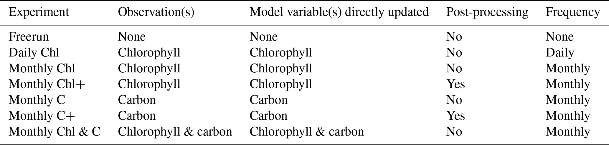
In these experiments, the “Daily Chl” experiment benefits from the high-frequency chlorophyll product. However, because only a monthly carbon product is available, monthly experiments are conducted for a fair comparison among different phytoplankton products. The “Monthly Chl & C” experiment is distinctive from other experiments. In this experiment, the state vector contains both phytoplankton chlorophyll and carbon. The DA update makes use of the correlation between these variables such that each variable is updated by both observation products.

The daily assimilation experiment is implemented by assimilating the daily chlorophyll observation at the start of each day. In monthly assimilation experiments, the assimilation takes place at the start of the day in the middle of each month. In all experiments, to ensure a gradual adjustment of the model simulation, an incremental analysis update (IAU) is used with a window of 1 d corresponding to 31 time steps where $\mathrm{1}/\mathrm{31}$ of the total increment of the model variable is applied for each time step.

5 Results

The aim of this study is to investigate the impact of assimilating the phytoplankton carbon product on the modelled marine ecosystems. To understand the impact of the product globally, each experiment is evaluated against the composite monthly observations described in Sect. 2.2. We further assess the influences of each experiment on marine ecosystem variables such as PFTs, zooplankton and gases such as pCO₂ and oxygen without validating these variables against in situ datasets in the present study.

5.1 Statistical scores

Here, the effects of the DA on assimilated variables are evaluated using the bias between the model and observations, the root mean squared differences (RMSDs), continuous rank probability score (CRPS), and ensemble spread. These scores can expose potential disagreements between different observations, the uncertainty, and reliability of the ensemble after DA.

5.1.1 Biases

The DA algorithm assumes that the forecasts and observations have no biases. However, this assumption is rarely met in real applications. Biases can exist both in observations and model forecasts for both carbon and chlorophyll. In model forecasts, the bias could be a result of inaccurate model parameters, simplified treatment of model processes and biased initial conditions (Mamnun et al., 2025). In addition to model forecast, the application of fixed C : N ratio could affect the biases. This fixed ratio can be viewed as a global average in both time and space; biases could only occur when the distribution of the spatially and temporally varying C : N ratio is not symmetric that leads to a ratio that is systematically either too large or too small (Tanioka et al., 2022). Quantifying biases in models and observations is non-trivial considering the limited availability of so-called anchor observations with negligible biases (Eyre, 2016; Fowler et al., 2023). Because DA methods assume uncorrelated forecast and observation errors, as a proxy, the bias can be revealed by the misfit between observations and the model forecast over multiple time steps used in the DA (Saha et al., 2014; Zuo et al., 2019; Barton et al., 2021; Mignac et al., 2025). The expectation of the misfit is zero in the absence of biases. Because the model parameters are not determined by the assimilated observations, this diagnostic can expose biases in the DA systems.

The misfits of logarithmic phytoplankton concentration represent the ratio between the model and observations, expressing relative differences that are independent of the absolute concentration values. Figure 2 shows the histogram of the misfits at the assimilation step during the 2-year experiment period. In Fig. 2a), chlorophyll is less biased than carbon, but the modelled chlorophyll will, in general, be increased by the DA, as demonstrated by the positive mean misfits (vertical lines). There are differences in the misfit between experiments, with the “Daily Chl” experiment showing a much smaller distribution than the “Monthly Chl” experiments. The magnitude of the mean misfit in “Daily Chl” is similar to the bias given by Ford et al. (2012). Without the high-frequency adjustments provided by daily assimilation, the misfit is less likely to approach zero, and instead exhibits an almost bimodal distribution. Notably, using the balancing scheme to update the phytoplankton carbon in the “Monthly Chl+” experiment slightly improves the expectation of the misfits in chlorophyll. This suggests that making direct changes in the primary composition of phytoplankton biomass in MEDUSA leads to more sustained changes in the model. This is consistent with the study conducted by (Ford and Barciela, 2017).

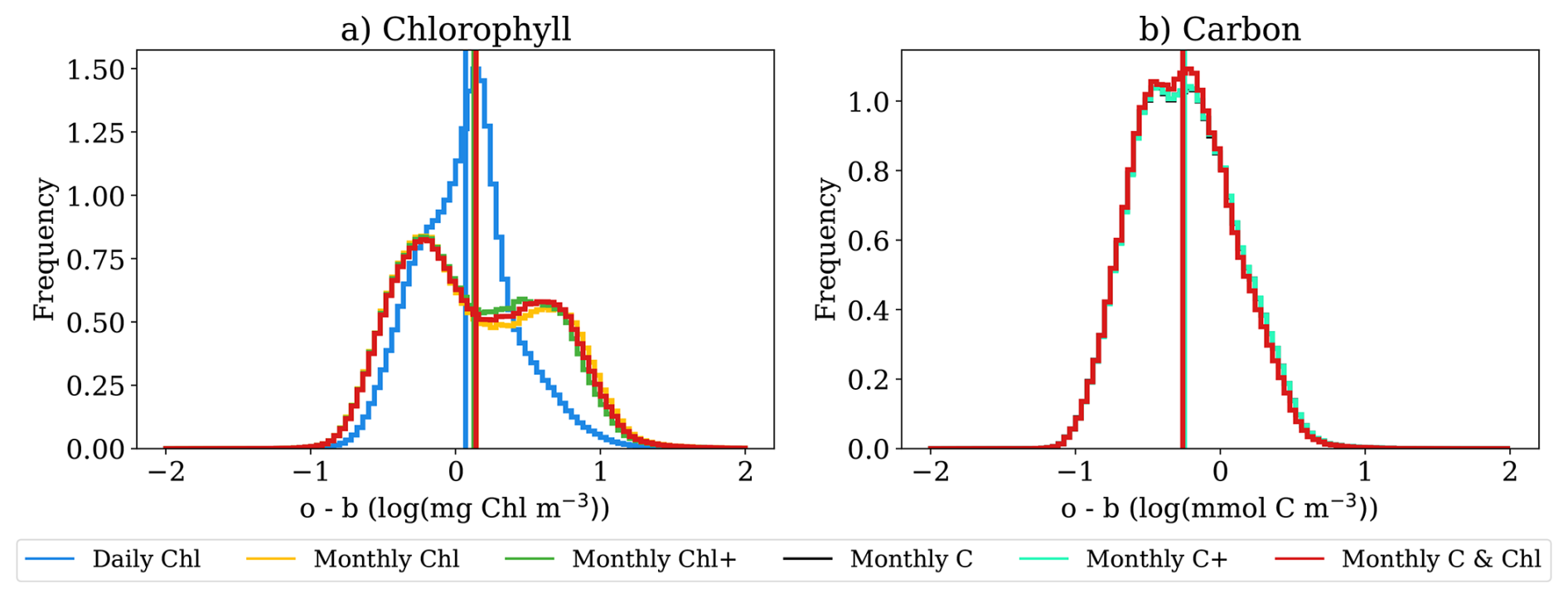
Figure 2 The histogram of the misfit between observations and forecast for log-transformed variables at the analysis step. Large observation and forecast misfits with low probability in (a) are neglected for display purposes. The mean of the misfits for each experiment is presented as vertical lines. This histogram was constructed by global instantaneous data used by DA over the entire experiment period.

In contrast, Fig. 2b shows a negative mean misfit for carbon, which implies that the modelled carbon is constantly reduced by the DA in all experiments assimilating carbon. Unlike in the “Monthly Chl+” experiment, updating chlorophyll in the “Monthly C+” experiment does not lead to an improved distribution of the misfits compared to the “Monthly C” experiment. Interestingly, compared to other experiments, the simultaneous assimilation of chlorophyll and carbon does not bring the averaged misfits closer to zero. This may suggest that the DA reaches a compromise between these observation products and the ratio of chlorophyll and carbon in observations differs from the model.

As suggested by the histogram, the errors of the modelled carbon and chlorophyll have different signs, and the use of a balancing scheme may struggle to correctly handle corrections for both chlorophyll and carbon. Considering the carbon data are derived based on chlorophyll data and their ratio is validated by Sathyendranath et al. (2020), in addition to the balancing scheme, the inconsistency of different signs may also arise from model errors. This could be driven by inaccurate modelling of the primary production, the loss of phytoplankton, and/or the coupling of chlorophyll and carbon, where the tendencies of chlorophyll and carbon are erroneous given modelled nutrient conditions. The assimilation of both products finds a compromise between the biased model and observation products.

5.1.2 Root mean square difference

The effect of the DA is here demonstrated by the root mean square difference (RMSD) between the ensemble mean of monthly averaged model forecasts and monthly composite observations. We first compare our model forecasts with independent in situ observations in Fig. 3 using the root mean squared difference of the logarithm of chlorophyll and carbon. The assessment is performed at observation locations using linear interpolation from model grid points. For convenience, the point observations are considered as monthly averaged values, which could cause additional errors in this evaluation. In Fig. 3a), the RMSD of the chlorophyll is calculated for the upper 50 m (around 18 model levels) of the ocean for model forecasts and observations. All experiments assimilating chlorophyll show reduced RMSD of chlorophyll compared to Freerun. Experiments assimilating carbon without chlorophyll show slightly increased RMSD of the chlorophyll. This suggests that assimilating carbon product does not necessarily improve chlorophyll in MEDUSA.

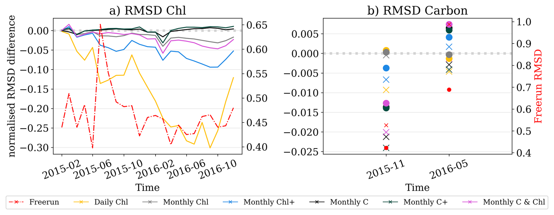
Figure 3 Differences in RMSD between DA experiments and Freerun normalised by the RMSD of Freerun between the logarithm of monthly model forecasts of and composites of chlorophyll from Argo and field campaign data from NAAMES on the left axis. The RMSD of Freerun is shown as a dashed red line on the right axis. The crosses represent comparisons with modelled total carbon while the dots represent comparisons with modelled non-diatom carbon.

The comparison with in situ carbon observations is more complicated because the carbon observations include only cells smaller than 64 µm. MEDUSA has no explicit definition of the size of diatom and non-diatom phytoplankton. Hence, in Fig. 3b), we compare the observations with model variables of both total phytoplankton (cross signs) and non-diatom phytoplankton (dot signs), which is considered to represent “small” phytoplankton. Assimilating chlorophyll has little impact on the RMSD of non-diatom carbon in November 2015. The RMSD of non-diatom carbon is reduced by assimilating carbon in November 2015 but the RMSD is increased in May 2016. The increased RMSD by assimilating carbon could be a result of post-processing and mismatch between the observations and PFTs, especially considering the seasonal dependence of the results. When comparing with total modelled carbon, assimilating carbon better constrains the carbon than assimilating chlorophyll regardless of season. Nevertheless, the impact of DA on the RMSD of carbon is smaller in November 2015 than in May 2016. For both carbon and chlorophyll, Daily Chl shows better performance than monthly assimilations. Overall, simultaneous assimilation of chlorophyll and carbon provides a balanced RMSD reduction compared to assimilating a single type of phytoplankton composition.

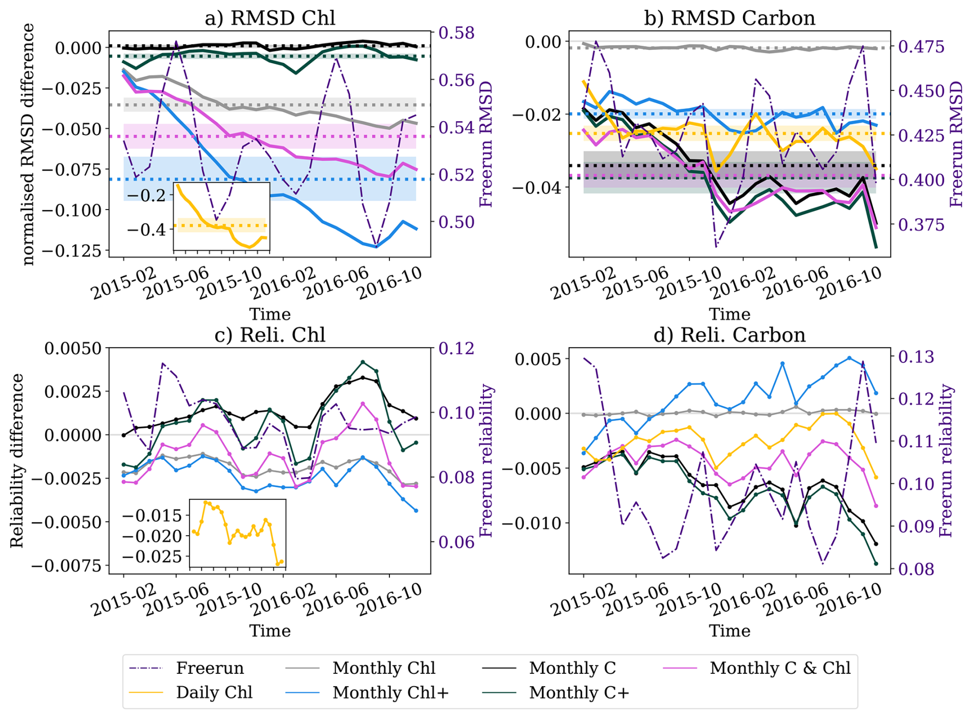
Figure 4 Upper row: time series of the RMSD of the ensemble mean of the logarithmic surface phytoplankton (a) chlorophyll and (b) carbon. The left axis shows the differences of RMSD between DA experiments and Freerun normalised by the RMSD of Freerun, and the right axis shows the RMSD of Freerun (red line). The light gray horizontal line is the zero line representing no global adjustments compared to Freerun. The inset in (a) is the RMSD difference of chlorophyll in the “Daily Chl” experiment. The horizontal dashed lines with shaded area are the temporal average of the RMSD, and the shaded area represents the 95 % confidence interval of the temporal average. Lower row: reliability score of the ensemble of surface phytoplankton (a) chlorophyll and (b) nitrogen compared against the assimilated observations derived from CRPS. The left axis is for the reliability differences between each DA experiment and Freerun, and the right axis is the reliability score of Freerun (red line). The inset in (c) is the reliability differences of chlorophyll in the “Daily Chl” experiment.

The assessment against in situ data is still limited by the spatial and temporal coverage. Hence, we further assess the results with assimilated satellite data in Fig. 4a–b. In Freerun, the RMSD of the logarithmic chlorophyll is higher than that of carbon. Because the RMSD of logarithmic concentration implicitly reflects the ratio between the ensemble mean and observations, the RMSD of the chlorophyll and the carbon can be compared directly. The lower RMSD of carbon suggests that it is simulated more accurately than chlorophyll in Freerun, potentially due to its role as a representation of phytoplankton biomass in the MEDUSA formulation. The RMSD of chlorophyll is comparable to that reported in Pradhan et al. (2019, 2020), despite of a different biogeochemical model. Here, the RMSD of chlorophyll peaks during the boreal spring and autumn. However, Pradhan et al. (2019) showed a higher RMS error in the boreal autumn than in spring, whereas our results show the opposite pattern, with larger RMSD in autumn. The differences can be explained by various factors including the model formulations, forcing, and ensemble size, which cannot be easily attributed. For example, Pradhan et al. (2019) used the MITgcm-REcoM2 model on a variable resolution from 0.38° to 2° with 20 ensemble members forced by Coordinated Ocean-Ice Reference Experiment (CORE). Our study used NEMO-MEDUSA on a fixed ORCA1 grid with 30 ensemble members forced by JRA-55. Apart from this, REcoM2 uses a varying stoichiometry, while MEDUSA uses fixed ratios. Moreover, our experiments coincide with a strong El Niño event. These could all lead to different responses to the seasonality of the results.

For each DA experiment, the RMSD is normalised by the RMSD of the Freerun experiment representing the ratio of the RMSD changes. In all experiments, the assimilation reduces RMSD, reflected by the negative difference of the normalised RMSD between the DA experiment and Freerun. The RMSD differences show a decreasing trend over the experiment period as the model state gradually adjusts towards the observations.

For chlorophyll, the largest RMSD reduction is obtained in the “Daily Chl” experiment, as expected. The RMSD is reduced up to more than 40 % at the end of the experiment period (see inset in Fig. 4a). With frequent adjustments to the model state, in the daily assimilation experiment, the carbon field is adjusted through modifying the light limitation of primary production in the model forecast, leading to a reduced RMSD of 2 %–4 % in carbon. Moreover, the daily chlorophyll assimilation outperforms monthly carbon assimilations with respect to the carbon field at the start of the assimilation.

The “Monthly Chl” experiment has a much smaller impact on chlorophyll compared to “Daily Chl”, and as a result has little influence on phytoplankton carbon biomass. It only reduces the RMSD of the chlorophyll by up to around 5 %. This result is consistent with the misfits statistics in Fig. 2. However, by updating the carbon, the RMSD of the “Monthly Chl+” is reduced by up to around 12 %, which is higher than the “Monthly Chl” experiment, as it is more able to make lasting adjustments to the marine ecosystem. But it is still not as effective as in the “Daily Chl” experiment. The “Monthly Chl+” experiment also results in RMSD reductions in carbon whereas the “Monthly Chl” experiment has a very limited impact on the RMSD of carbon.

In the “Monthly C” and “Monthly C+” experiments, in which carbon observations are assimilated, the RMSD reduction of the chlorophyll field is the lowest. In particular, without chlorophyll update, the “Monthly C” experiment results in almost no chlorophyll improvements, and can lead to deteriorated RMSD compared to the Freerun. For carbon the RMSD reduction in the “Monthly C”, “Monthly C+”, and “Monthly Chl & C” experiments is similar, and is even larger across the year than the “Daily Chl” experiment. Lastly, even though showing less RMSD reduction in chlorophyll than the “Daily Chl” and “Monthly Chl+”, assimilating both datasets in the “Monthly Chl & C” experiment shows the most balanced performance of all monthly experiments with respect to both variables. This shows the benefits of utilising both datasets even if we do not account for their correlations. Moreover, the improvements from “Monthly Chl+” show that updating both phytoplankton constituents is an effective and necessary approach when only chlorophyll is assimilated. The monthly carbon assimilation presents further reduced RMSD in carbon concentrations than only assimilating chlorophyll. The RMSD reduction suggests the need for direct assimilation of both phytoplankton constituents to achieve balanced adjustments and the potential for significant improvements with a more frequent and sophisticated phytoplankton carbon product.

5.1.3 Uncertainties of the ensemble system

In addition to the RMSD of the ensemble mean, a reliable ensemble DA system is expected to represent the probability of the occurrence of a given state, i.e. the uncertainty of the system. In a perfectly reliable ensemble, by definition, such an ensemble will have an probability distribution function identical to the true probability distribution (Leutbecher and Palmer, 2008; Rodwell et al., 2016). Here, the true probability distribution is represented by the probability distribution of the assimilated observations as calculated by the reliability score of the continuous ranked probability score (CRPS). The CRPS is widely used to diagnose ensemble forecasts (Hersbach, 2000), representing the differences between the cumulative probability of the distribution given by the model ensemble and observations. The CRPS can be decomposed into reliability and resolution scores. In a perfectly reliable ensemble, the reliability score is zero, and the ensemble represents the true uncertainty of the model simulations. The reliability score increases with less reliable ensemble. The reliability score of the CRPS is evaluated on a grid point by grid point basis. As the DA does not guarantee improved reliability by construction, this metric helps us evaluate the accuracy of quantified uncertainty from each experiment.

Figure 4c–d focuses on the reliability score under the assumption that the climatology distributions are given by observations. The non-zero reliability score shows that the ensemble is not perfectly reliable. This highlights the challenge of achieving a reliable global ensemble system and underscores the need for further investigation into quantifying uncertainty in MEDUSA. The ensemble used in this study is in general under-dispersive. This could lead to smaller adjustments than an optimal system. The ensemble reliability can benefit from perturbations in atmosphere forcing and spatially and temporally dependent parameters. However, this will require further careful tuning and possible modifications to the model itself. Such a challenge is also investigated by Anugerahanti et al. (2018) and Mamnun et al. (2022). For the chlorophyll field, daily chlorophyll assimilation continuously adjusts the chlorophyll ensemble, leading to the best reliability score. In the case of monthly DA, assimilating chlorophyll in general shows an improved reliability score compared to Freerun. In comparison, the “Monthly C” and “Monthly C+” experiments could lead to a less reliable chlorophyll ensemble regardless of the chlorophyll update.

For carbon, whilst the “Daily Chl” experiment improves the reliability of the carbon field, the “Monthly Chl” and “Monthly Chl+” experiments deteriorate the carbon reliability. All experiments with carbon assimilation lead to a more reliable carbon ensemble than any experiments without. The fact that assimilating a single observation product could potentially lead to a less reliable ensemble in the other variable demonstrates a benefit for assimilating multiple products in our ensemble system.

It is worth noting that, among all experiments, the simultaneous assimilation of chlorophyll and carbon does not necessarily lead to the most reliable ensemble. The less reliable ensemble is likely an effect of the contradictory influence of these two types of observations in comparison to Freerun. Yet, the DA can provide a compromise between the two observation datasets.

Besides reliability, the ensemble also provides uncertainty information of the model forecasts, which is typically estimated by the ensemble spread, i.e., the standard deviation of the ensemble. By construction of the LESTKF, the analysis ensemble should have a smaller total ensemble spread over the grid points compared to the forecast ensemble as the ensemble spread is a proxy of the error of the ensemble forecast in a reliable ensemble system (Leutbecher and Palmer, 2008). However, this does not mean that the analysis spread is smaller than the forecast spread for every grid point. Instead, the LESTKF reduces the total ensemble spread compared to the total forecast spread across the domain.

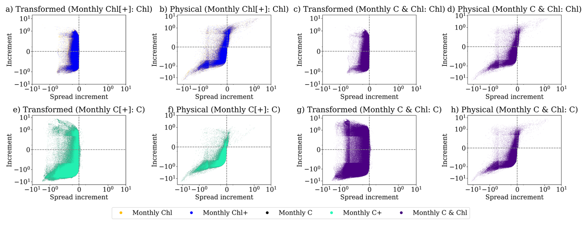
Figure 5 Scatter plot of the ensemble mean increment against the ensemble spread increment on a log scale. Here, the LESTKF is performed on transformed variables following the Gaussian distribution, and the physical values are the ensemble mean and standard deviation of the phytoplankton concentrations. First row: Chlorophyll increment and spread increment; second row: carbon increment and spread increment. The “Monthly Chl[+]” represents both “Monthly Chl” and “Monthly Chl+” experiments, and “Monthly C[+]” represents both “Monthly C” and “Monthly C+” experiments; the variable is given after the colon.

The log-transformation of the concentrations described in Sect. 3 leads to a Gaussian distribution, which is used in the LESTKF. Figure 5 shows increments for these transformed variables as well as for the actual values. As expected, in Fig. 5a, c, e, g, the ensemble spread of the log-transformed variables is reduced by the LESTKF, i.e. the increment (differences between the analysis and forecast spread) is overall negative. However, when transformed back into physical space the DA leads to increased ensemble spread at some grid points. For a Gaussian distribution, the mean and standard deviation are independent of each other, whilst for a lognormal distribution this is not the case. Thus, even if the DA reduced the ensemble spread for the log-transformed variables, the corresponding ensemble spread of the actual variables can increase due to their log-normal distribution. This effect is shown in Fig. 5b, d, f, h, where a clear relationship between the change of the ensemble spread and the ensemble mean is visible. The increased ensemble spread corresponds closely to the increased ensemble mean value. This is a feature of the log-normal distribution, where the mean and spread of the distribution are related. Namely, when the DA increases the ensemble mean value, the ensemble spread of the actual variable can be increased even if the spread of the log-transformed variable is decreased. The ensemble spread can still be reduced if the observations are accurate enough to sufficiently suppress the spread of the log-transformed variable as is visible in Eq. (2). This emphasises the importance of accurate observations following a log-normal distribution, especially in high-concentration regions. When such high accuracy observations are not available, we postulate that post-processing may be necessary to prevent unphysical ensemble members.

In the “Monthly C” and “Monthly C+” experiments of Fig. 5e, the negative carbon bias from Fig. 2 is evident compared to the chlorophyll experiments in Fig. 5a. In contrast, the increment of the carbon in the “Monthly Chl & C” experiment of Fig. 5g shows more similarity with the “Monthly Chl[+]” of Fig. 5a than the “Monthly C[+]” experiment of Fig. 5e. In addition to the interaction between phytoplankton chlorophyll and carbon, the similarity might be because the chlorophyll observations have lower uncertainty than carbon observations, so that the DA assimilates more information from the chlorophyll product. This suggests that, even if the phytoplankton products yield contradictory increments, the marine ecosystem prediction can benefit from the simultaneous assimilation of both observations for its ability to optimally combine different sources of observations.

5.2 Model adjustments

Besides the statistical metrics, to understand the spatial adjustments of the global system, we now compare the adjustments made to surface phytoplankton chlorophyll and carbon in different experiments.

5.2.1 Adjustments in total phytoplankton

As shown in Fig. 6, Freerun and the observations capture similar spatial patterns, with higher values in polar and subpolar regions of both hemispheres, coastal regions and the eastern equatorial Pacific than in other regions. Such spatial pattern is consistent with other studies, e.g., Yool et al. (2013) and Ford (2021). The higher resolution of the observations captures more features, with the model showing higher chlorophyll concentration around the eastern equatorial Pacific region, Southern Ocean, the Benguela Current region, and some of the sub-polar regions of the northern hemisphere. Yet, the model does not capture the high chlorophyll concentration in open ocean areas such as the Atlantic and Indian oceans, and around some of the coastal regions of Antarctica. These all contribute to the overall positive misfits between observations and the model discussed in Sect. 5.1.1.

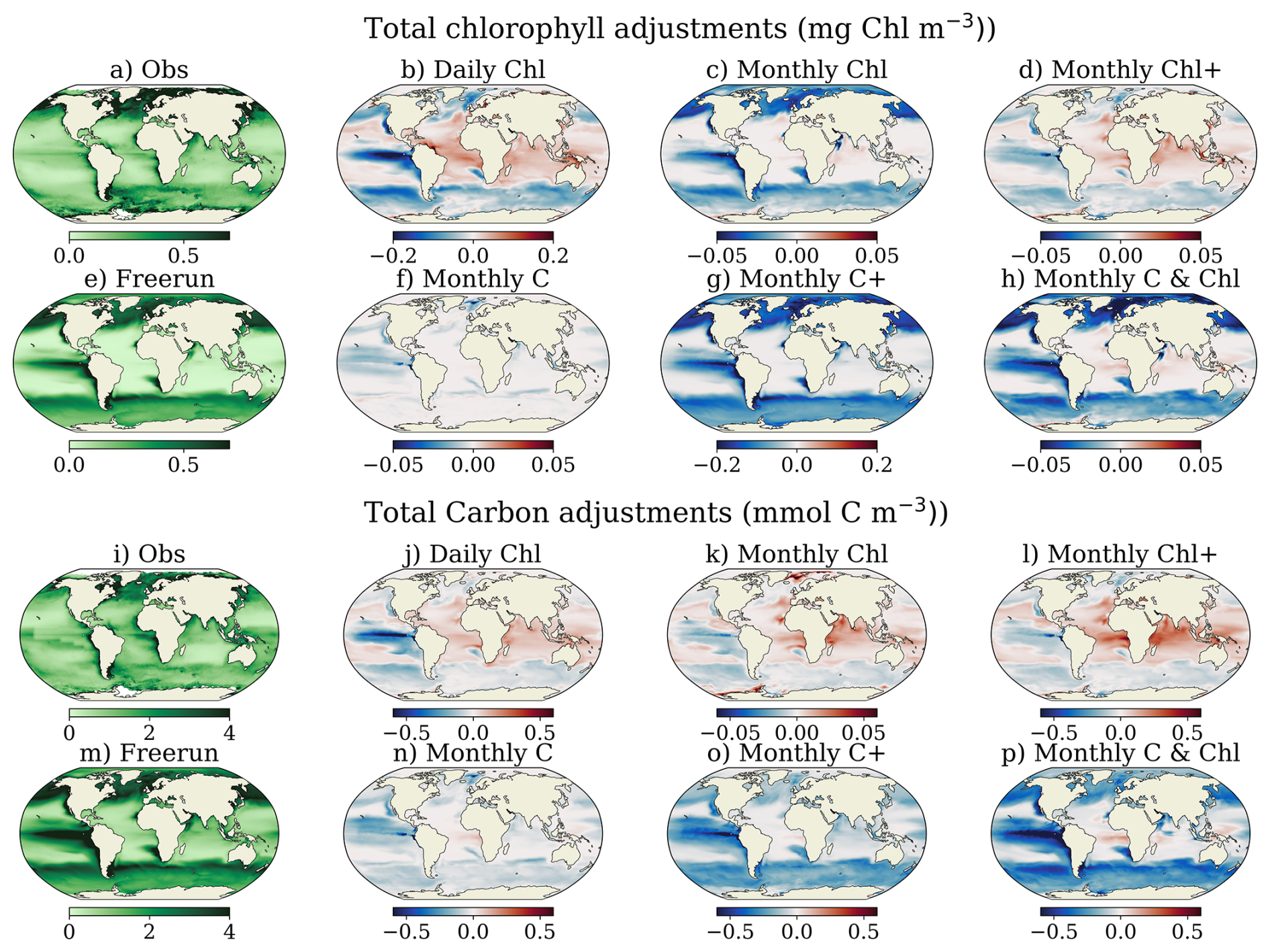
Figure 6 The phytoplankton chlorophyll concentration in (a) observation and Freerun (e) and the differences between the DA experiments and Freerun experiment in (b)–(d) and (f)–(h). The phytoplankton carbon concentration in (i) observation and Freerun (m) and the differences between the DA experiments and Freerun experiment in (j)–(l) and (n)–(p). The differences are computed based on the temporal mean of the ensemble mean of monthly model output over the experiment period. Note that some experiments use a different colour scale.

Similarly, in Fig. 6i and m, the modelled carbon also has lower concentrations in the open ocean and higher concentration in the eastern equatorial Pacific than the observations. The modelled carbon also shows spatial patterns similar to chlorophyll in the Benguela Current region and the equatorial Atlantic due to biased ocean upwelling (Yool et al., 2013). However, in high-concentration regions, the modelled carbon exhibits excessive values, spanning a wider latitudinal range than the modelled chlorophyll in several areas, such as the eastern equatorial and South Pacific Ocean. These patterns are distinct from the low carbon concentrations simulated in the open ocean basins when compared with satellite observations. The difference in spatial patterns demonstrate that a single observation product cannot fully represent the phytoplankton biomass, highlighting the need for carbon products. It is also worth noting that a strong El Niño occurred during our experiment period which had a strong impact on the eastern Equatorial Pacific. The differences between observations and Freerun may reflect the modelling capability of the El Niño event as well. This could imply that results from Freerun and other experiments in the eastern Pacific region may not be generalised to years without El Niño events.

In the “Daily Chl” experiment, the frequent assimilation leads to one of the strongest adjustments compared to other experiments, as exhibited in Fig. 6b). These adjustments show a similar spatial pattern as the error correction in Pradhan et al. (2019). The frequent assimilation also results in a similar spatial pattern of adjustments in carbon (Fig. 6b and j). However, opposite signs of adjustment exist; e.g. in the Nordic Seas, the DA reduces chlorophyll but increases carbon. This increase in carbon is at odds with observations. This contradiction is related to a weak increase in chlorophyll during the spring bloom combined with a strong reduction in other seasons. This reduction has limited impact on the carbon, as the region is predominantly nutrient limited.

Similarly, the “Monthly Chl” and “Monthly C” experiments also only assimilate one type of observation without updating other phytoplankton constituents via post-processing. The less frequent adjustments in these experiments lead to smaller adjustments as shown by Fig. 6c, f, k and n. In “Monthly Chl”, the weak model response of carbon to the monthly chlorophyll assimilation limits the adjustment of chlorophyll itself, as indicated by its colour scale. The changes in chlorophyll are not maintained over the one-month forecast, and this effect is amplified by the lack of a direct influence on carbon. Compared to “Monthly Chl+” in Fig. 6d, the stronger decreases and weaker increases of chlorophyll in “Monthly Chl” result from the MEDUSA formulation where a modified slope of the photosynthesis–irradiance curve, scaled by the chlorophyll-to-biomass ratio represented by carbon. The “Monthly C” experiment results in the weakest adjustment of chlorophyll among all experiments due to the infrequent adjustments and lack of direct DA update of chlorophyll.

When both carbon and chlorophyll are updated, the DA adjustments become stronger. Modifying the chlorophyll based on the carbon adjustments leads to the strongest adjustments of the chlorophyll among all experiments, as exhibited by its colour scale in Fig. 6g). In regions with decreased chlorophyll and carbon, the DA adjustments of “Monthly C+”, “Monthly Chl+” and “Monthly Chl & C” experiments share similar spatial patterns. There are regional differences between experiments in increases of phytoplankton. For example, the “Monthly Chl+” experiment shows strong increases in both the chlorophyll and carbon in the Black, Timor and Mediterranean Seas, low- and mid-latitude marine zones, except in the eastern equatorial Pacific and along the coasts of subpolar regions. These increases are absent in the “Monthly C+” experiment, with instead a strong reduction of the carbon and chlorophyll in the Black, Timor and Mediterranean Sea. These are regions where the differences between chlorophyll and carbon observations are strongest. Compared to the experiments that assimilate chlorophyll observations, this also suggests an unrealistic modification of the chlorophyll based on the carbon update.

Disagreements still exist in the simultaneous assimilation of both observations. However, in this case, these disagreements do not arise from changes in individual PFTs or from assumptions in the post-processing approach. Instead, the chlorophyll and carbon corrections largely depend on their respective observational datasets.

5.2.2 Adjustments in phytoplankton functional types

In MEDUSA, phytoplankton are represented as individual state variables of diatom and non-diatom functional types. These size classes are updated by post-processing in the DA system based on the ratio between the forecast PFT field and the total phytoplankton field as described in Sect. 3.1. Figures 7 and 8 show the changes to each functional type for chlorophyll and carbon respectively. The diatom functional group tends to have a lower concentration than the non-diatom group for both chlorophyll and carbon content, with spatial patterns similar to the total concentration (Fig. 6).

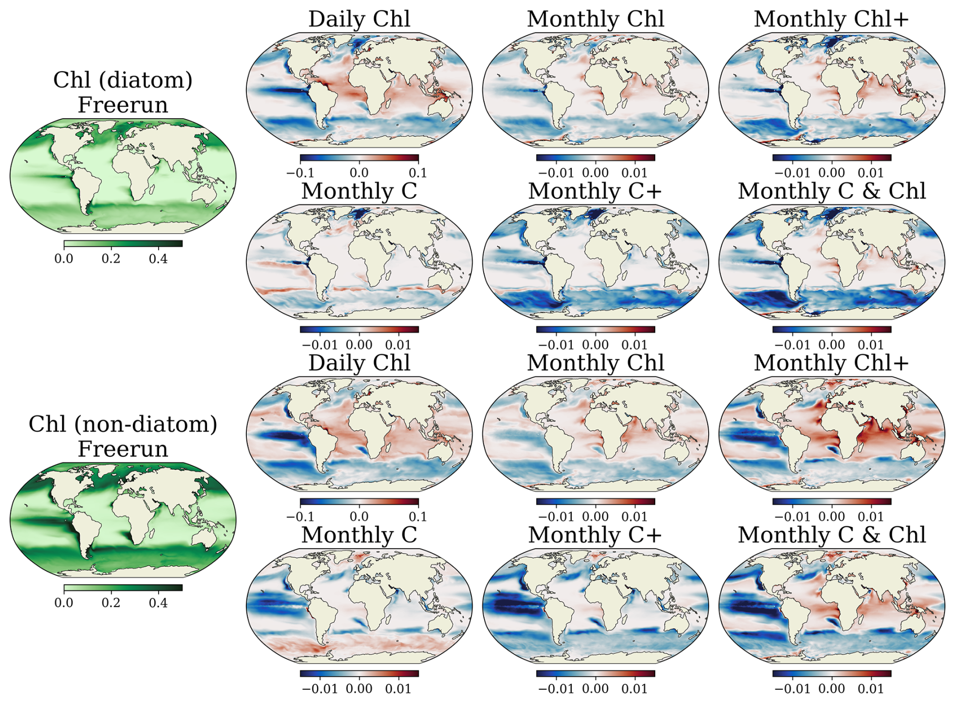
Figure 7 Similar to Fig. 6 but for phytoplankton chlorophyll concentration (mg Chl m⁻³) of diatom and non-diatom classes. Note that the “Daily Chl” experiment has a different colour scale from other experiments.

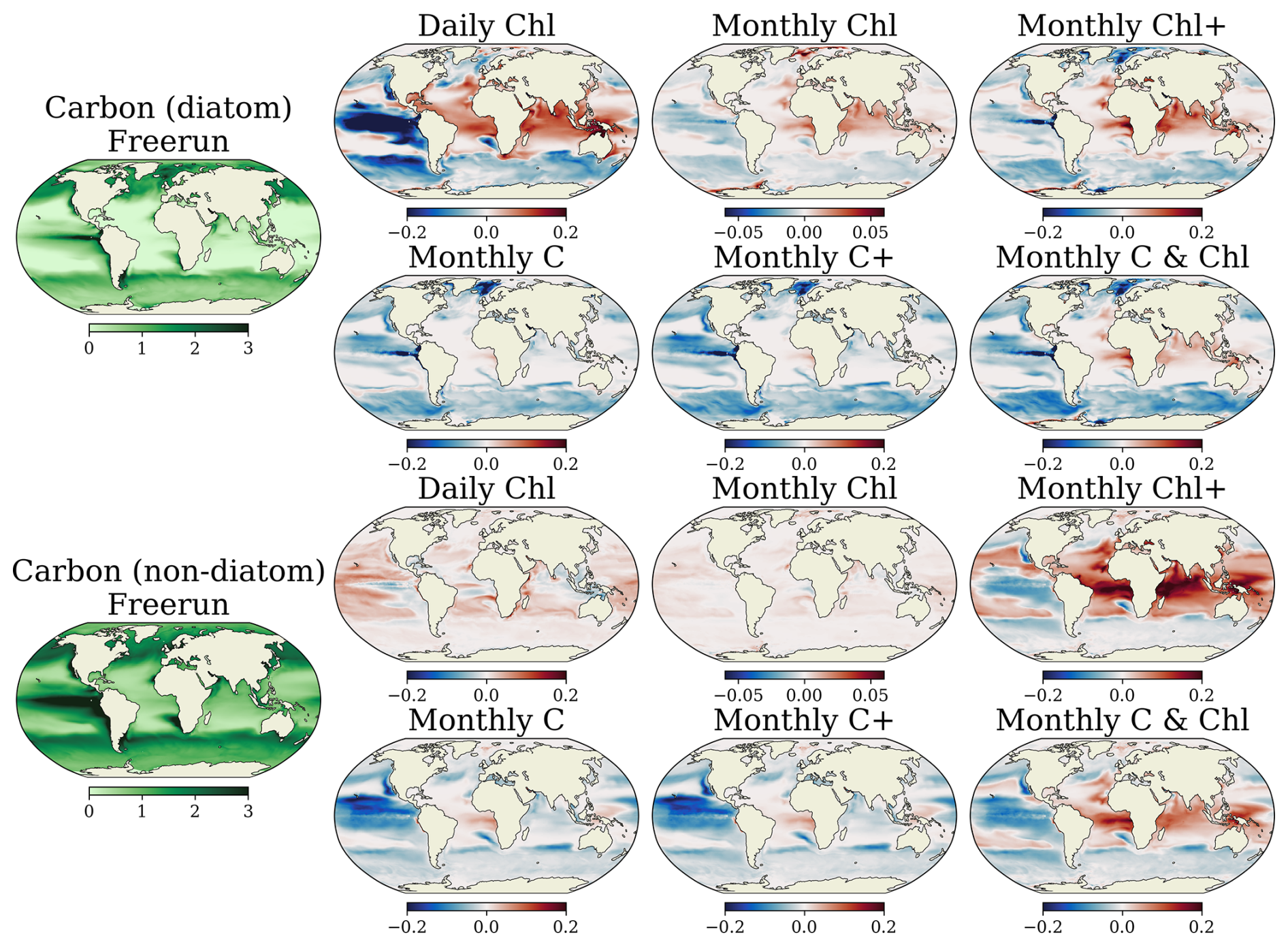
Figure 8 Similar to Fig. 6 but for phytoplankton nitrogen concentration (mmol C m⁻³) of diatom and non-diatom classes. Note that the “Monthly Chl” experiment has a different colour scale than other experiments.

Although the spatial pattern of phytoplankton functional types in the Freerun experiment are similar to that of the total phytoplankton, DA adjustments do not necessarily follow the same spatial pattern as their total concentration. These differences are evident in the cases where only one of the chlorophyll or carbon fields is updated.

In the “Daily Chl” and “Monthly Chl” experiments, even though the spatial pattern of each chlorophyll size class follows the adjustments of the total chlorophyll, the carbon adjustments show a more complex spatial pattern. This is because in these experiments, the size classes of chlorophyll are updated based on the DA increments, but the carbon is adjusted through model responses to those increments. Diatom carbon responds similarly to chlorophyll, with strong decreases of phytoplankton in the eastern equatorial Pacific, whilst non-diatoms have a much weaker response. In the Southern Ocean and along the Alaska and California currents, the model shows increased non-diatom carbon due to increased primary production as a response to decreased chlorophyll. This is due to how MEDUSA handles the relationship, with decreased chlorophyll reducing the ratio between phytoplankton chlorophyll and carbon. Since the relationship between non-diatom growth rate and light limitation is non-linear, decreased chlorophyll leads to increases in primary production.

In the “Monthly C” experiment, we expect that the chlorophyll will largely follow the phytoplankton biomass changes. However, Figs. 7 and 8 show that both diatom and non-diatom chlorophyll can exhibit contrasting adjustments. These distinct features are evident in the Southern Ocean, the Benguela current and around the North Atlantic drift. These differences are a result of the model formulation of MEDUSA, where the chlorophyll tendency is related to the carbon tendency by a complex function of the primary production and various scaling factors.

The different signs between chlorophyll and carbon adjustments disappear when post-processing is applied in “Monthly Chl+” and “Monthly C+” experiments. In these experiments, the diatom and non-diatom components of chlorophyll and carbon are adjusted proportionally based on the forecast towards the assimilated observations. In the “Monthly C+” experiment, the model responses can become dominant compared to DA increments. There is increased non-diatom carbon in the Nordic Seas due to increased primary production, whilst diatom carbon reflects the decrease seen in the total carbon field. This type of model response occurs for all experiments that assimilate the carbon product.

As discussed in Sect. 5.1, different observation products can lead to contrasting phytoplankton increments. By assimilating both in the “Monthly Chl & C” experiment, we see enhanced model adjustments in PFTs that reflect spatial patterns from both sets of observations compared to “Monthly Chl+” and “Monthly C+” experiments.

5.3 Seasonality

Phytoplankton have a strong seasonal variation, as seen in Fig. 4. Evaluation of the seasonal adjustments from DA can reveal changes in key processes in marine ecosystem due to different assimilation strategies. It is worth discussing the impact of DA on the spatial pattern of phytoplankton in each season beyond the year-round climatology. As shown in Sect. 5.2.1, observations and each experiment have their own climatology. Here, we focus on the impact of DA on the seasonal anomalies without the climatological mean.

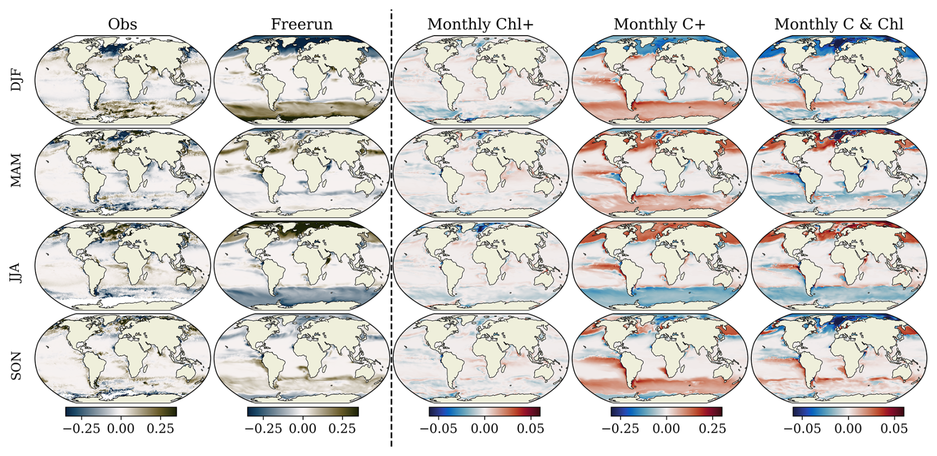
Figure 9 First two columns: seasonal anomalies of chlorophyll concentration (mg Chl m⁻³) relative to the year-round climatology of observations and the Freerun experiment. Last three columns: differences in seasonal anomalies between the DA experiments and the Freerun experiment (positive values indicate increased anomalies, negative values indicate decreased anomalies). For each experiment, seasonal anomalies are computed relative to that experiment's own year-round climatology. Note: the “Monthly C+” experiment uses a different colour scale than the others.

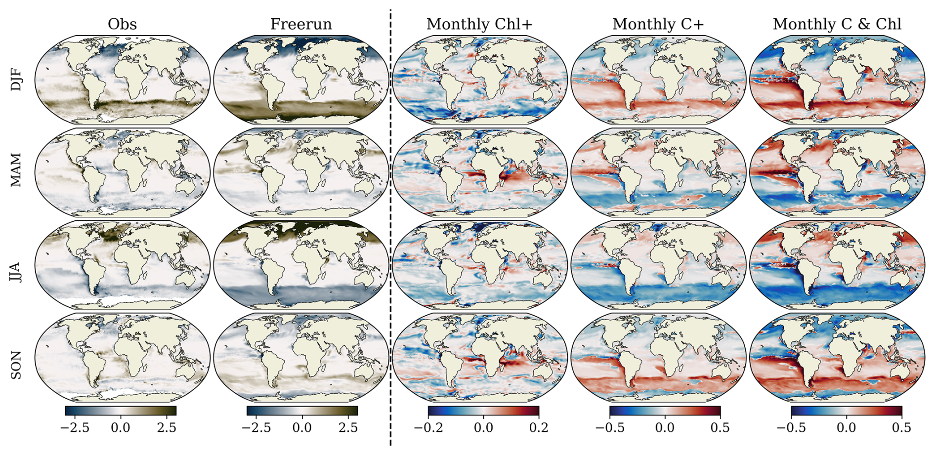
Figure 10 First two columns: seasonal anomalies of carbon concentration (mmol C m⁻³) relative to the year-round climatology of observations and the Freerun experiment. Last three columns: differences in seasonal anomalies between the DA experiments and the Freerun experiment (positive values indicate increased anomalies, negative values indicate decreased anomalies). For each experiment, seasonal anomalies are computed relative to that experiment's own year-round climatology. Note: the “Monthly Chl+” experiment uses a different colour scale than the others.

For the sake of simplicity, we only discuss the spatial adjustments in each season for the DA experiments that update both chlorophyll and carbon. The Freerun experiment generally captures the seasonal variations in Figs. 9 and 10, albeit with some bias. Consistent with Yool et al. (2013, 2021), the positive seasonal anomaly of both carbon and chlorophyll shifts to the northern hemisphere in boreal summer and shifts to the southern hemisphere in austral summer, following the seasonal variation of the radiation conditions. The Freerun also successfully captures regions where the seasonal anomalies of the chlorophyll and carbon are different. For example, in boreal winter, the model represents opposite anomalies in carbon and chlorophyll in the mid-latitude Atlantic, the east Pacific, the Indian Ocean, and the south Pacific. Yet, there are regions where the Freerun experiment disagrees with the observations. For instance, in boreal spring a positive anomaly of phytoplankton extends toward higher latitudes in the North Atlantic that is not present in the observations. The model also fails to capture the correct sign of the seasonal anomaly in observations around the Nordic Seas and Arctic Ocean in boreal autumn for carbon and in boreal summer and autumn for chlorophyll. This suggests that, in addition to year-round biases discussed in Sect. 5.1, the Freerun also shows errors in seasonal biases.

Compared to the seasonal variation of the freerun experiment, each DA experiment shows different changes in its seasonal anomalies. In Fig. 9, although the “Monthly C+” and “Monthly Chl & C” experiments show similar spatial patterns of seasonal chlorophyll adjustments in many regions, e.g., in mid-latitude and around the Equator, the “Monthly Chl & C” experiment also exhibits features characteristic of “Monthly Chl+” where only chlorophyll is assimilated. For example, the reduced seasonal anomaly in the Southern Ocean in boreal winter and spring aligns with “Monthly Chl+” instead of “Monthly C+”. This demonstrates that neither carbon nor chlorophyll alone can represent the seasonal cycle of phytoplankton biomass. Furthermore, chlorophyll adjustments are larger in the “Monthly C+” experiment than in the “Monthly Chl & C” experiment. The positive seasonal anomaly adjustments in “Monthly C+” indicate that assimilating carbon increases the positive and reduces the negative chlorophyll seasonal anomaly, suggesting a stronger seasonal variation than in the Freerun.

Similar to chlorophyll, the carbon anomaly is generally similar in the “Monthly C+” and “Monthly Chl & C” experiments as shown in Fig. 10. In contrast, the “Monthly Chl+” experiment not only shows the smallest adjustments (see colourbar in Fig. 10) but also fails to show a strengthened seasonal anomaly when the carbon product is assimilated. This suggests that assimilating chlorophyll alone with post-processing could deteriorate the seasonality of modelled global phytoplankton in MEDUSA. When carbon and chlorophyll products are assimilated simultaneously, the strengthened seasonal anomalies become stronger than those obtained by assimilating the carbon product alone.

Comparing Fig. 10 with Fig. 9, the seasonal anomalies are adjusted differently for the chlorophyll and carbon fields for the same experiment. For example, during the boreal spring, assimilating both carbon and chlorophyll reduces the carbon seasonal anomalies near the Arctic, but a strengthened seasonal anomaly is displayed in the same region. The different adjustments show that relying on multiple PFT observations improves the statistics of phytoplankton seasonal variations in ocean biogeochemical reanalyses.

5.4 Effects on zooplankton, inorganic carbon and oxygen cycles

Even though the ensemble DA system only adjusts phytoplankton, these changes of phytoplankton impact the entire marine ecosystem model, including zooplankton, nutrients and detritus. As with phytoplankton, MEDUSA represents zooplankton with two functional types: meso- and micro-zooplankton, where mesozooplankton are more abundant due to grazing on a wider variety of prey (Fig. 11). The spatial distribution of Freerun exhibits similar features as in other studies using MEDUSA, e.g. Yool et al. (2013); Petrik et al. (2022). In the DA experiments, the spatial pattern of zooplankton adjustments closely follow the phytoplankton adjustments. The spatial pattern of microzooplankton changes are largely identical to the non-diatom phytoplankton in Fig. 8 because they graze on detritus and non-diatom phytoplankton. Mesozooplankton graze on both microzooplankton and diatom phytoplankton, so the spatial pattern is more aligned with the total phytoplankton adjustments in Fig. 6. These changes are consistent across all DA experiments and follow the model formulation.

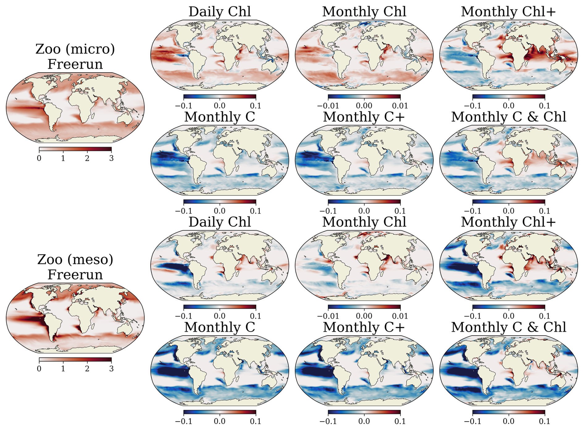
Figure 11 The micro- (ZMI) and meso- (ZME) zooplankton concentration (mmol C m⁻³) of Freerun (first column) and the differences in phytoplankton nitrogen between the DA experiments and the Freerun experiments. The differences are computed based on the temporal mean of the ensemble mean of monthly model output over the experiment period.

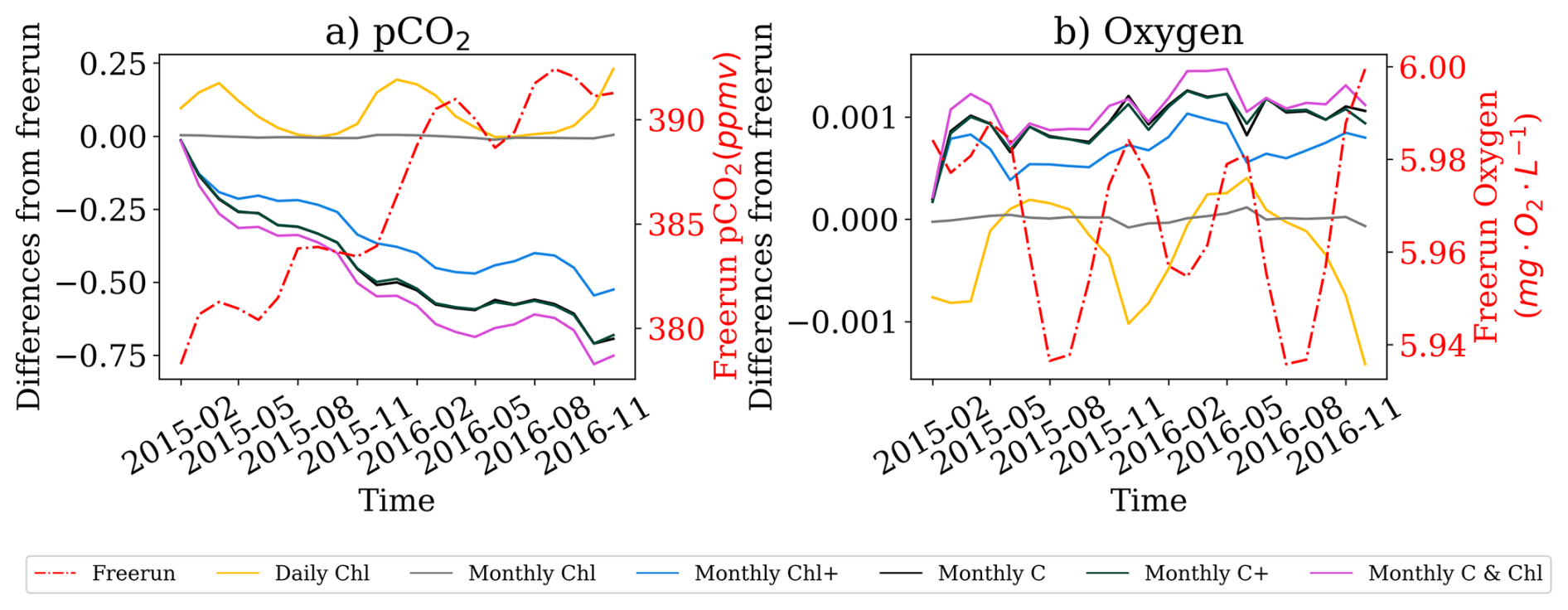
Figure 12 The time series of globally averaged ocean surface pCO₂ (left) and oxygen (right). Shown are Freerun (red line on right axis) and the difference from Freerun for each DA experiment.

The time series of the Freerun experiment in Fig. 12 represents the globally averaged ocean surface pCO₂, which has a seasonal variation but a clear upward trend. The pCO₂ is within the range of pCO₂ given by other studies (e.g., Takahashi et al., 2009; Carroll et al., 2020). The troughs of the seasonal variation correspond to the peaks in phytoplankton blooms. Changes to the globally averaged pCO₂ are minimal in the “Monthly Chl” experiment, but in the “Daily Chl” experiment, the adjustments in the marine ecosystem lead to increased pCO₂ growth. The increase is related to the strong reduction of phytoplankton around the eastern equatorial Pacific and the increased respiratory activities in zooplankton seen in Fig. 11. In other experiments, the pCO₂ concentration increases slower than the Freerun experiment over time. With updates of carbon based on chlorophyll observations in the “Monthly Chl+” experiment, the level of slowdown of pCO₂ increase is not as strong as experiments assimilating phytoplankton carbon. The “Monthly C” and “Monthly C+” experiments show similar adjustments in pCO₂, suggesting that the update of chlorophyll has little impact at monthly resolution. When both chlorophyll and carbon observations are assimilated, the pCO₂ increase is slowed down the most among all experiments. This suggests that the assimilation of carbon observations reduces the pCO₂ at the ocean surface by reducing global phytoplankton carbon.

Unlike pCO₂, the ocean surface oxygen concentration shows a strong seasonal variation without an obvious trend, which could be a result of the different equilibration timescales of O₂ from pCO₂. The “Monthly Chl” experiment has little impact on the oxygen level. However, the “Daily Chl” experiment shows reduced oxygen concentration while other experiments show increased oxygen at the ocean surface. The “Monthly Chl+” experiment shows a moderate increase, while the “Monthly Chl & C” experiment shows the highest level of increase in oxygen. The increased oxygen in these experiments is a result of less consumption of oxygen from the reduced zooplankton. This reduction in oxygen consumption exceeds the reduction in oxygen generation from photosynthesis due to reduced phytoplankton.

These results show that even though the “Monthly Chl & C” experiment does not show the highest RMSD reduction in Sect. 5.1.2, the experiment has a stronger impact on the ocean pCO₂ and oxygen than assimilating only one type of observations. Besides, we expect a sustained impact with time due to the biases in the marine ecosystem model. This highlights the need to assimilate observations at high temporal frequency, and to include both observational datasets to maximise the impact on the marine ecosystem.

6 Conclusions

In this study, we evaluated the effect of assimilating a novel satellite phytoplankton carbon product in comparison to the traditional phytoplankton chlorophyll dataset. To perform the evaluation, a global marine ecosystem ensemble DA system, PDAF-NEMO-MEDUSA, was constructed using the DA software framework, PDAF.

In all DA experiments, both phytoplankton carbon and chlorophyll become more globally aligned with observations of phytoplankton carbon and chlorophyll. These improvements arise mainly from increments with the same sign when assimilating either observation type in a majority of the global ocean. Despite these alignments, the overall misfits between the model and observations differ in sign for carbon and chlorophyll. This is because these alignments do not hold in regions with contrasting increments when different observation products are assimilated. This shows the disparities between phytoplankton chlorophyll and carbon. Assimilating both observational datasets simultaneously can account for the contrasting signs.

When only one product is assimilated, adjustments to other phytoplankton components are primarily driven by the model or by post-processing based on increments of the assimilated variables. The majority of these adjustments lead to a similar pattern of increments as the dataset that is being assimilated. However, these adjustments to variables other than the assimilated product could also lead to increased differences with observations and can deteriorate the seasonal variation in some regions. For example, in Monthly Chl+, the seasonality of phytoplankton carbon could deteriorate. This finding could suggest deteriorated seasonality for other DA systems assimilating chlorophyll alone, but, considering the seasonal discrepancy of RMSD with Pradhan et al. (2019), this could also be model and period dependent, which requires further investigations. When no post-processing is used, the model cannot accurately adjust itself to changes, particularly at monthly resolution. In the case of assimilating the widely used chlorophyll observation, only adjusting the light limitation of primary production does not ensure a changed phytoplankton biomass because of the intricate interactions between nutrients and zooplankton. The update from post-processing shows that inferring increments of other variables is not always reliable as well, especially when increments are apportioned to PFTs that do not change proportionally to each other.

Any assimilation experiment has an impact beyond phytoplankton, with the assimilation of a single product potentially having a deteriorating response in other parts of the ecosystem such as the zooplankton, pCO₂ and oxygen. The largest response was seen when assimilating both products.

Our results demonstrate that the simultaneous assimilation of carbon products and chlorophyll can yield more balanced adjustments in phytoplankton biomass. Nevertheless, these adjustments may vary depending on the formulations of individual marine ecosystem models. In MEDUSA, carbon and nitrogen are assumed to have a fixed stoichiometric relationship. By contrast, more complex models such as ERSEM (Butenschön et al., 2016) or quota-based models like REcoM2 (Schourup-Kristensen et al., 2014) may exhibit distinct responses to perturbations in carbon or chlorophyll. For example, Ciavatta et al. (2025) compared responses to assimilating chlorophyll in models of different complexities. It is of interest to make such comparisons for carbon products. We hypothesise that in more complex models, where the representation of carbon and chlorophyll dynamics is more sophisticated, the DA is likely to produce more robust ecosystem responses.

In this study, we also investigated the performance of the ensemble DA system. The more frequent daily chlorophyll assimilation improved the reliability of the ensemble compared to monthly assimilation experiments, where the low temporal resolution impacted the ability of the model to tend towards the observed state. Due to the assumption of a log-normal distribution for phytoplankton biomass, the DA system required a statistical transformation to perform the DA using a Gaussian distribution. However, the DA does not necessarily decrease the ensemble uncertainty due to the dependence of the variance on the mean value of the log-normal distribution, even though the resulting analysis is better aligned with the observation than the forecast. From a technical point of view, for future work, the ensemble DA system can be improved through better ensemble generation with more reliable perturbations for ocean forcing and biogeochemical parameters. A reliable ensemble could further lead to multivariate DA increments that could perform better than the post-processing scheme used here as demonstrated by Pradhan et al. (2019).

There are potential further benefits of assimilating even more information about the phytoplankton. From a DA perspective, assimilating the phytoplankton carbon product still requires further investigation, including better quantification of the observation error and assessment of the correlation between the carbon and chlorophyll products. It is of interest to understand the impact of daily assimilation of phytoplankton carbon observations similar to operational biogeochemical DA where chlorophyll is assimilated daily. This would require a daily product in line with the current chlorophyll product. Moreover, independent observations will be needed to quantitatively validate the DA system in addition to phytoplankton chlorophyll and carbon. For example, BGC-Argo floats, the Surface Ocean CO₂ Atlas (SOCAT) or World Ocean Atlas datasets could be used for nutrients, oxygen, and carbonate variables. Furthermore, this study follows the common practice of operational DA systems by only assimilating satellite ocean colour (Skákala et al., 2025). This means that updates to the subsurface structure are not as accurate as assimilating profiles of marine ecosystem variables such as BGC-Argo data. Hence, it is also of interest to investigate a DA system that assimilates both vertical profiles along with ocean colour data.

Appendix A: Ensemble perturbations

In an ensemble data assimilation system, the forecast error distribution is estimated from the forecast ensemble. The forecast errors come from the initial condition and the epistemic uncertainties arising from physical and biogeochemical parameters. Limited by the computational cost, 30 ensemble members are used in this configuration. As the ensemble is used to estimate the error covariance of the forecast, the limited ensemble size unavoidably leads to sampling errors that could lead to reduced ensemble spread and filter divergence. To overcome these issues, an inflation of 5 %, implemented by a forgetting factor of 0.95 (Nerger et al., 2012), is applied to inflate the ensemble during the analysis step.

In this study, the initial conditions of surface chlorophyll and nitrogen as well as 3D ocean temperature and salinity are perturbed. The perturbation of these fields are sampled from a Gaussian distribution. The covariance matrix of the Gaussian distribution is approximated from a model trajectory from January–March of 2000–2005. In this case, each time step is considered as a sample following the Gaussian distribution. This approach assumes that the uncertainty of model initial condition can be captured by model variability over this period. The ensemble is generated by the 2nd-order exact sampling Pham (2001) provided by PDAF from sampled error covariances with zero mean. The ensemble is run for one month without any DA allowing for improved physical consistency among model variables by model adjustments.

To take the physical model error into account, STochasticOcean physics PACKage (STOPACK, Storto and Andriopoulos, 2021), is used to perturb the physical parametrisations. The stochastic physics package provides both stochastically perturbed parameters (SPP) and a stochastic kinetic energy backscatter (SKEB) scheme. The SPP scheme perturbs a suite of dynamical and physical parameters in NEMO while the SKEB scheme transfers the eddy kinetic energy from unresolved scales to resolved scales which mimics an inversed energy cascade. In the SPP scheme, a selection of parameters is perturbed where the perturbations follow a log-normal distribution as given in Table A1. The SKEB scheme only perturbs the eddy kinetic energy with a first-order autoregressive model with a standard deviation of 1 and a time decorrelation scale of 1.

Table A1 Perturbed parameters and standard deviation used in SPP scheme in STOPACK.

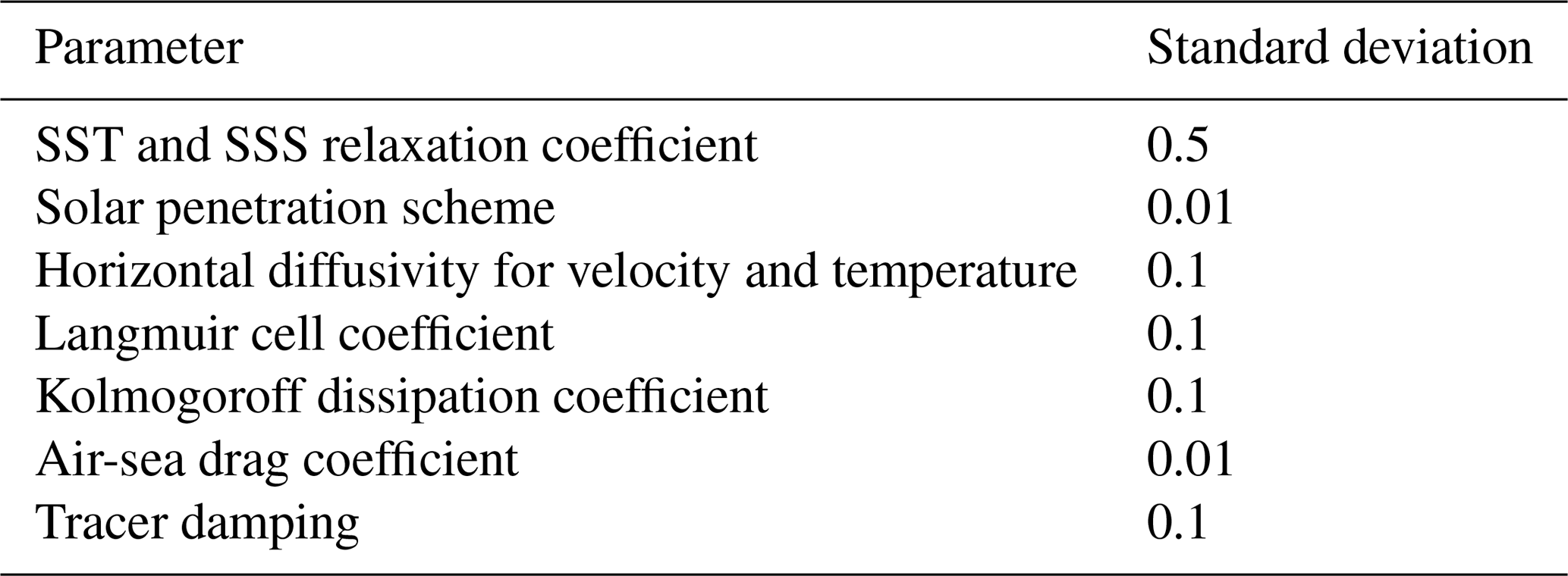
Table A2 Perturbed parameters in MEDUSA. The last column is the constraints of parameters after the sampling from a uniform distribution.

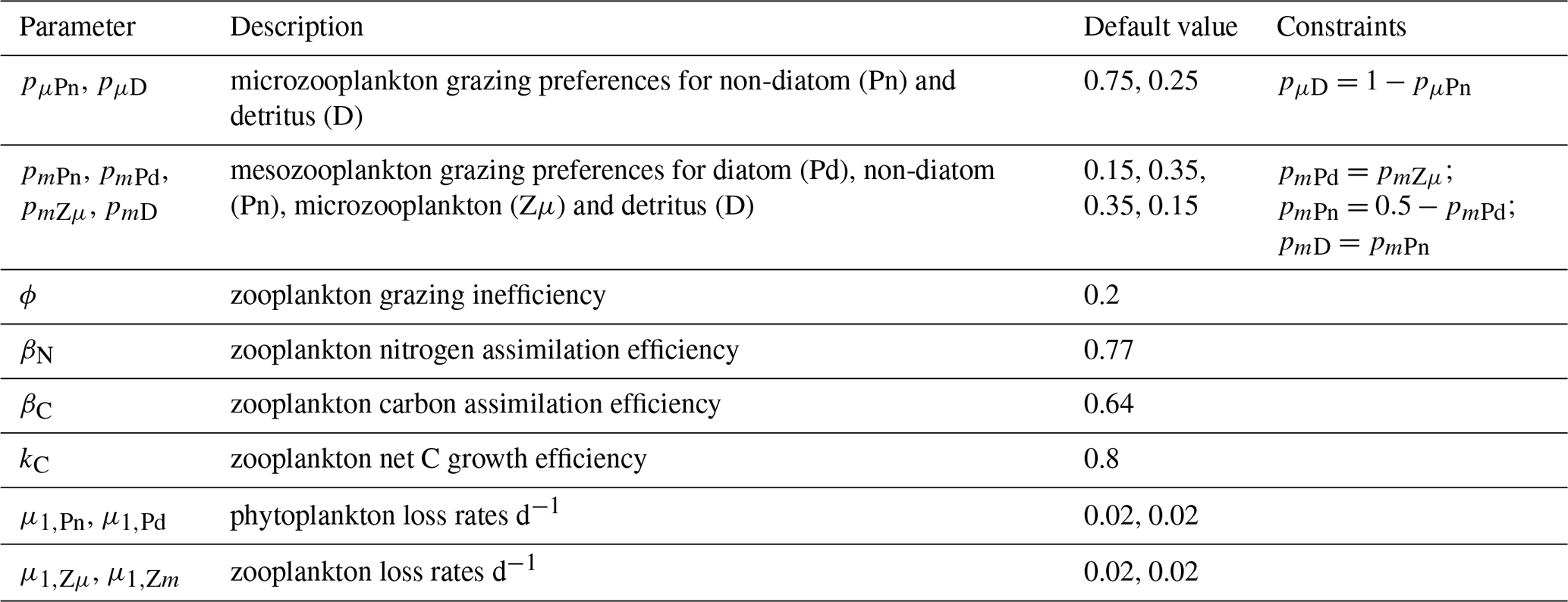
Further, a total of 11 biogeochemical parameters have been selected to be perturbed, as shown in Table A2. The parameters are first sampled from a uniform distribution 𝒰(0.8p,1.2p), where p is the default parameter value. Constraints are then imposed shown in the last column of Table A2.