GLIDE-SOL: a GPU-accelerated global lightweight infrastructure for diagnostic environmental modeling with SOLWEIG

GLIDE-SOL is a fully scripted and globally re-deployable Python workflow that operationalizes SOLWEIG for rapid and repeatable thermal-comfort mapping across diverse urban environments. GLIDE-SOL is built on the SOLWEIG radiative balance libraries, but rewrites the surrounding system – including automated input generation, the execution engine, and post-processing – so that the model can be driven by globally available datasets and executed efficiently on GPUs. All inputs (terrain, building morphology, canopy height, land cover, and meteorology) are automatically derived from global products, eliminating local preprocessing while enabling consistent applications from neighborhood-scale analyses to city-wide and multi-city experiments. In addition, GLIDE-SOL introduces lightweight physical diagnostics to improve realism when driven by coarse meteorological forcing, targeting key urban controls on wind and near-surface temperature.

The workflow incorporates two physical augmentations: (i) roughness- and obstacle-based directional wind attenuation to approximate near-surface ventilation; and (ii) diagnostic temperature adjustments that combine a simple urban heat island (UHI) cycle with an elevation-based correction using high-resolution DEM information, to better capture nocturnal warming and local lapse-rate effects.

To scale to large metropolitan areas, GLIDE-SOL uses explicit domain tiling with cross-tile synchronization to preserve radiative consistency across tile boundaries, enabling meter-scale simulations over tens to hundreds of square kilometers without sacrificing reproducibility. Daily outputs (24 radiative and meteorological fields) are stored as compressed GeoTIFFs to reduce disk usage and accelerate downstream processing.

GLIDE-SOL is implemented through three reproducible components: an automated global-input generator; a SOLWEIG execution engine with coordinated tiling; and a post-processing module for systematic sampling, time-series extraction, and visualization. An operational demonstration in Dortmund, using hourly measurements from 25 urban and peri-urban stations and simulations run at 2 m grid spacing between August 2024 and December 2025, shows that incorporating wind attenuation and the diagnostic temperature corrections substantially improves UTCI performance (RMSE reduced from 8.09 to 2.84 °C), alongside improvements in T_mrt, air temperature, and wind speed simulations.

By integrating harmonized global inputs with physics-based diagnostics, GPU acceleration, and scalable tiling, GLIDE-SOL supports applications such as operational UTCI nowcasting, retrospective and climatological analyses of heat stress, sensitivity tests of urban morphology and greening strategies, and coordinated multi-city experiments requiring consistent modeling protocols.

1 Introduction

Fast and transferable urban thermal-comfort modeling is increasingly required for climate-adaptation planning, operational heat warnings, and systematic inter- and intra-city assessments. Exposure to urban heat stress is shaped by large-scale atmospheric conditions and fine-scale variations in radiation, wind, urban form, and surface cover, with pronounced differences between neighborhoods, street canyons, and open spaces (Emmanuel and Fernando, 2007; Mayer et al., 2008). Urban heat islands, particularly at night, and uneven daytime exposure to high radiant loads and locally reduced wind speeds contribute to elevated heat-stress risk (Oke et al., 2017). Radiant load, often expressed through mean radiant temperature (T_mrt), is a crucial meteorological driver of human energy balance and thermal comfort during warm, clear conditions (Mayer and Höppe, 1987; Thorsson et al., 2007). T_mrt is a key input to bio-climatic indices such as the Physiological Equivalent Temperature (PET) and Universal Thermal Climate Index (UTCI) (Höppe, 1999; Fiala et al., 2012; Jendritzky et al., 2012), which combine radiation, air temperature, humidity, and wind speed into a single thermal-stress metric (Cheng et al., 2012).

T_mrt arises from the net shortwave and long-wave radiation fluxes from all surrounding surfaces and the sky. While intra-urban air-temperature differences are often modest during the day, T_mrt can exhibit strong spatial variability over distances of only a few meters (Lindberg and Grimmond, 2011a, b; Thorsson et al., 2011; Middel and Krayenhoff, 2019). These microscale variations are primarily driven by shadow patterns created by buildings, trees, and topography, as well as by differences in surface radiative and thermal properties such as albedo, emissivity, and heat capacity (Thorsson et al., 2007; Konarska et al., 2014; Lindberg et al., 2016). The SOLWEIG (SOlar and LongWave Environmental Irradiance Geometry) (Lindberg et al., 2008) model is widely used to estimate T_mrt and related thermal-comfort indices in complex urban environments. It resolves shortwave and longwave radiation fluxes in three dimensions and has been applied to analyze the influence of urban geometry, ground surfaces, and vegetation on outdoor thermal comfort in a variety of climates, and validated against ground observations (Lindberg and Grimmond, 2011a, b; Briegel et al., 2024; Buo et al., 2023). SOLWEIG is also integrated in the Urban Multi-scale Environmental Predictor (UMEP) (Lindberg et al., 2018), which provides a QGIS-based environment for linking urban-climate models with geospatial data to support climate services, heat-risk assessments, and planning applications. Despite its strong theoretical foundation and broad adoption in case studies, SOLWEIG has not yet matured into a globally operational tool.

Several persistent barriers limit the wider deployment of SOLWEIG for city-wide or multi-city applications. First, realistic setups typically require detailed, locally assembled input data: high-resolution digital elevation/surface models, building land cover, footprints and heights, vegetation structure, and representative meteorological forcing (Jänicke et al., 2016; Zonato et al., 2020). These inputs are often derived from local LiDAR campaigns, city-specific GIS databases, or bespoke classifications, which are not uniformly available across regions. Second, microscale radiative models can be computationally demanding when applied at meter-scale resolution over large urban domains or long simulation periods (Toparlar et al., 2017; Briegel et al., 2024). Third, near-surface wind is frequently prescribed from single meteorological stations or coarse reanalyses that do not explicitly account for building-induced sheltering and channeling, even though wind strongly modulates thermal comfort (Cionco, 1972; Chu and Wang, 2025). CFD models such as ENVI-met and PALM-4U can resolve pedestrian-level wind and temperature fields (Simon, 2016; Maronga et al., 2020), but their computational cost generally restricts their use to micro-scale domains or limited simulation periods.

In parallel, global geospatial and meteorological datasets have advanced to the point where they can serve as a common input backbone for urban climate applications. ESA WorldCover provides 10 m global land-cover classes suitable for distinguishing major urban and vegetated surfaces (Zanaga et al., 2022). On the terrain side, MERIT DEM (Yamazaki et al., 2017) offers harmonized global elevation information at 3 arcsec (∼90 m) resolution, forming a consistent basis for topographic inputs.

Complementing these terrain-only products, a new generation of open building datasets has emerged, providing both footprints and 3D attributes essential for urban climate modeling. Microsoft global building footprints (Microsoft, 2026), Overture Maps building footprints (Overture Maps Foundation, 2026), and GlobalBuildingAtlas LoD1 buildings (Zhu et al., 2025) provide a practical multi-source basis for assembling building footprints across regions with very different input-data availability. Building-height attribution can then be supported by products such as GlobalBuildingAtlas and OpenBuildingMap (Oostwegel et al., 2025).

At the same time, global canopy-height products have also matured rapidly: very-high-resolution (1 m) tree-height maps derived from self-supervised deep learning trained on airborne LiDAR (Tolan et al., 2024), the global canopy height model by Lang et al. (2023) at 10 m resolution, and the GEDI-based Canopy Height Mapper (Potapov et al., 2021), which delivers canopy heights at 30 m resolution through a Google Earth Engine workflow, collectively provide consistent estimates of vegetation height and distribution. Together, these resources supply a coherent global basis for representing not only terrain and buildings but also the three-dimensional distribution of urban and peri-urban vegetation. In dense urban settings, however, narrow streets, building shadows, and mixed pixels can still affect canopy detection. The resulting tree layer is therefore used here as a globally consistent approximation of urban vegetation structure, while local mapping errors are treated as part of the input-data uncertainty.

On the meteorological side, the ERA5 reanalysis provides globally consistent, hourly atmospheric fields (Hersbach et al., 2020). However, its coarse resolution inherently limits the representation of mesoscale and, especially, urban-scale processes: even when dynamically down-scaled, ERA5 tends to smooth local thermal gradients and fails to capture city-specific features and extreme conditions (Adinolfi et al., 2023). Platforms such as Google Earth Engine enable planetary-scale access and processing of these datasets in a reproducible, scriptable manner (Gorelick et al., 2017).

Recent studies demonstrate that city-wide, building-resolving thermal-comfort mapping with SOLWEIG and UMEP is now feasible using scripted workflows. Jänicke et al. (2016) performed a city-wide analysis of T_mrt at building resolution, while more recent work has produced high-resolution thermal exposure and shade maps to support cool-corridor planning (Buo et al., 2023). A key recent example is the study by Lindberg et al. (2025), who applied UMEP–SOLWEIG at 2 m resolution across Stockholm, Gothenburg, and Malmö to quantify how building density, tree fraction, and ground cover shape PET, UTCI, T_mrt, and pedestrian wind speed during heatwaves.

At the same time, GPU-based approaches to urban heat mapping have shown that large-domain, high-resolution simulations can be substantially accelerated. Li and Wang (2021) report over 99 % speed-up in computing city-scale heat-exposure metrics from high-resolution surface data. Yang et al. (2023) achieve near–real-time urban LES using a multi-GPU framework that preserves building-resolving detail. Similarly, the multi-scale City-LES v2.0 model (Kusaka et al., 2024) exploits GPU clusters to efficiently couple mesoscale and microscale LES, enabling long-duration, building-explicit simulations with full radiative calculations. Likewise, Li et al. (2024) employs GPU-accelerated computation to assess heat sensitivity and vulnerability across major U.S. cities, demonstrating that large-scale exposure analyses can now be carried out with operationally feasible runtimes.

In addition, recent open-source work has demonstrated how the core SOLWEIG radiative-geometry and time-stepping calculations can be refactored for GPU execution. SOLWEIG-GPU provides a Python implementation that runs SOLWEIG (v2022a) on GPUs via a simple API, CLI, or GUI, and targets meter-scale, city-scale domains by combining domain tiling with GPU-parallelized computation of SVF, T_mrt, shadows, and UTCI (while wall height and wall aspect remain CPU-side and are parallelized across cores) (Kamath et al., 2026).

Reported benchmarks show substantial acceleration for the SVF + UTCI core: for tile sizes of 1000×1000, 1500×1500, and 2000×2000 cells, runtimes decrease from 1187, 3322, and 6487 s on a CPU workstation to 47, 105, and 158 s on an NVIDIA A6000 GPU, corresponding to approximately 25×, 32×, and 41× speed-ups. This work served as a practical reference point for the GPU-oriented design choices adopted in GLIDE-SOL.

The goal of GLIDE-SOL (Global Lightweight Infrastructure for Diagnostic Environmental modeling with SOLWEIG) is to transform SOLWEIG from a case-specific research tool into a reproducible, globally deployable workflow. GLIDE-SOL rests on three pillars. First, all required input data are obtained from globally or regionally available datasets – including ESA WorldCover (Zanaga et al., 2022), MERIT DEM (Yamazaki et al., 2017), GlobalBuildingAtlas (Zhu et al., 2025), and ERA5 accessed and processed via Google Earth Engine (Gorelick et al., 2017; Hersbach et al., 2020) – and automatically transformed into SOLWEIG-ready rasters. Second, GLIDE-SOL incorporates diagnostic physical modules designed to compensate for limitations of coarse meteorological forcing in urban settings: a Röckle-style directional wind-attenuation scheme (Röckle, 1990; Bernard et al., 2023) and a simple urban heat island adjustment informed by urban-climate theory (Theeuwes et al., 2016). Third, GLIDE-SOL targets scalability and computational efficiency through GPU-accelerated radiative geometry and explicit domain tiling. Entire cities, including large metropolitan areas spanning tens to hundreds of square kilometers, can thus be simulated at meter-scale resolution, with daily outputs stored as compressed GeoTIFFs for efficient downstream analysis.

In this paper, we document the GLIDE-SOL workflow and demonstrate its capabilities in Dortmund, Germany, using a dense observational network of 25 urban and peri-urban stations between August 2024 and December 2025. Simulations are conducted at 2 m grid spacing over the full metropolitan area. We first describe the automated pre-processing pipeline and its use of global datasets, then outline the SOLWEIG configuration, diagnostic wind and Urban Heat Island (UHI) modules, and GPU tiling strategy, and finally present an evaluation of hourly UTCI, T_mrt, air temperature, and wind speed against observations. Beyond reporting skill metrics, we discuss operational aspects such as wall-clock time and memory usage, and consider how a global-input, SOLWEIG-based workflow can support operational heat-risk assessment, climatological analysis, urban-planning evaluation, and coordinated multi-city modeling experiments.

2 Materials and methods

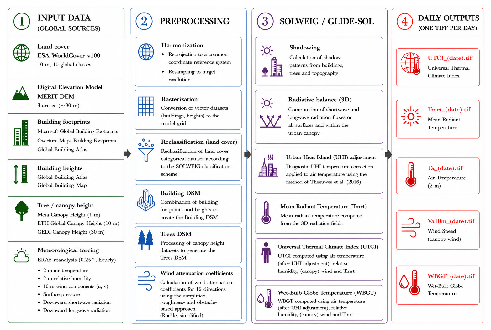
This section presents the end-to-end methodology of the GLIDE-SOL framework. We first describe the SOLWEIG Preprocessor, which automatically builds a co-registered spatial input stack (rasters and vectors) and harmonizes ERA5 meteorological forcing into SOLWEIG-ready formats. We then outline the GPU-accelerated execution strategy, including tiling, memory management, and CPU/GPU responsibilities for scalable hourly simulations. Finally, we detail the additional physical parameterizations introduced in this work (diagnostic UHI cycle, elevation bias correction, and wind reduction coefficients) that improve realism while preserving a fully reproducible, script-driven workflow based on globally available data sources and standardized processing steps. Figure 1 provides an overview of the complete pipeline.

Figure 1 Workflow of the GLIDE-SOL framework.

2.1 Overview of the SOLWEIG core

SOLWEIG (SOlar and LongWave Environmental Irradiance Geometry) is a three-dimensional radiative model developed to estimate mean radiant temperature (T_mrt) and related thermal-comfort quantities from urban geometry, vegetation, sun position, and near-surface meteorological forcing (Lindberg et al., 2008; Lindberg and Grimmond, 2011a, b; Lindberg et al., 2018; Wallenberg et al., 2020, 2023). At each time step, the model combines direct, diffuse, and reflected shortwave radiation with longwave exchange from sky, ground, walls, and vegetation to resolve the radiative environment experienced by a pedestrian, from which T_mrt and derived indices such as UTCI can be computed. This representation has been widely used in urban-climate and outdoor-comfort studies, including intercomparisons with other microclimate models and evaluations against observations (Aydin et al., 2019; Briegel et al., 2024).

In GLIDE-SOL, this logic is preserved but organized into an explicit, GPU-oriented execution sequence. The solver loads the static morphology layers (Building_DSM, DEM, Trees, Landuse, Walls, and Aspect), computes total and directional sky-view factors (SVF), evaluates building and vegetation shadow masks, and then advances the hourly SOLWEIG radiation balance on each tile before computing T_mrt, air temperature adjustments, wind speed, and UTCI. This implementation mirrors the standard SOLWEIG radiative structure while exposing the geometry and radiation terms needed for tiled GPU execution in GLIDE-SOL.

For the Dortmund experiments we used the SOLWEIG v2022a radiative core with the anisotropic sky schemes for both diffuse shortwave and longwave radiation. Diffuse shortwave radiation is represented with the Perez et al. (1993) sky-luminance distribution as implemented in SOLWEIG: instead of assuming an equal diffuse radiance over the visible sky, the diffuse component is distributed over sky-vault patches according to solar position, clearness, and brightness. This affects the directional shortwave load received by a pedestrian, particularly in partly obstructed urban canyons. Longwave irradiance is treated with the anisotropic parameterization introduced for SOLWEIG v2022a, in which sky longwave emission is also resolved over sky patches rather than prescribed as a spatially uniform hemispheric term (Wallenberg et al., 2020, 2023). The human receiver is represented as a cylinder, consistent with the SOLWEIG configuration used for pedestrian T_mrt.

2.2 Automated inputs with SOLWEIG Preprocessor

The input builder assembles a reproducible stack of rasters and vectors from a latitude/longitude seed, relying on globally accessible sources. The emphasis is to avoid bespoke digitization and to keep decisions transparent and scriptable:

• –

  Grid and Coordinate Reference System (CRS): starting from a target latitude–longitude pair, the script automatically selects the appropriate UTM zone, builds a geographic bounding box, and defines a regular metric grid (square pixels). All subsequent rasters (land cover, DEM, trees, buildings, wind coefficients) are reprojected and resampled onto this common grid, so that masking, sampling, and spatial statistics are perfectly co-registered.

• –

  Land cover, WorldCover reclassification, and elevation: the script downloads ESA WorldCover 2020 version 2 (Zanaga et al., 2022) for the study area and reclassifies it into a small set of land-use classes tailored to SOLWEIG:

  • 1.

    urban (WorldCover code 50),

  • 2.

    vegetation (default class for all other codes),

  • 3.

    water (WorldCover codes 80, 70, 90),

  • 4.

    bare & sand (WorldCover code 60).

  The reclassified raster is saved as Landuse.tif. In parallel, the script downloads and clips a digital elevation model (DEM), using a high-resolution global product such as MERIT DEM (Yamazaki et al., 2017, 90 m), and resamples it to the same grid as DEM.tif. The DEM is later used to apply an elevation-based correction to ERA5 2 m air temperature (Sect. 2.4.2).

• –

  Urban form: the current preprocessor uses a multi-source building workflow. Building footprints can be assembled from a configurable priority order of Microsoft global building footprints (Microsoft, 2026), Overture Maps (Overture Maps Foundation, 2026), and GlobalBuildingAtlas (Zhu et al., 2025). The workflow first cleans each source, builds a non-duplicated footprint baseline by priority, and then assigns roof heights independently from the available height products. Height attribution is sampled in priority order from GlobalBuildingAtlas (Zhu et al., 2025) and OpenBuildingMap (Oostwegel et al., 2025); remaining gaps are filled with the domain median roof height, and a small lower bound of 2 m is enforced to avoid unrealistically low buildings. The resulting footprint and height vectors are rasterized on the common grid and stacked with land-use information, yielding Buildings.tif (building footprints) and Building_DSM.tif, computed as DEM + roof height.

• –

  Trees: a high-resolution tree-canopy DSM is downloaded via Google Earth Engine from global canopy-height products, trying three sources in order of priority: (i) Meta Forest Monitoring/CanopyHeight (Tolan et al., 2024, 1 m), (ii) ETH Global Canopy Height 2020 (Lang et al., 2023, 10 m), and (iii) a GEDI-based product (Potapov et al., 2021, 30 m). The selected canopy DSM is mosaicked and rasterized on the common grid to produce Trees.tif, representing tree and woody vegetation cover and height across the domain.

• –

  Wind coefficients: using Buildings.tif, Trees.tif, the script computes 12 directional wind-sheltering rasters WindCoeff_dirXXX.tif (one for each 30° sector) based on a Röckle-style directional wind-reduction model. The 30° discretization was selected as a pragmatic compromise: it is fine enough to represent the main directional anisotropy of the street and building layout while keeping pre-processing cost and storage moderate. For each wind direction, the sheltering effect of buildings and trees is represented through upwind and downwind attenuation zones, then smoothed (e.g. via Gaussian filtering) and clipped to the SOLWEIG domain to avoid artifacts (Sect. 2.4.3).

• –

  Meteorology: meteorological forcing is harmonized from ERA5 reanalysis (Hersbach et al., 2020), retrieved via Google Earth Engine (Gorelick et al., 2017). In the current GLIDE-SOL workflow, ERA5 is sampled at the centre of the model domain and converted into a single city-scale background time series. The forcing includes near-surface air temperature and humidity, surface pressure, 10 m wind components, aerodynamic roughness length, surface altitude, and downward shortwave radiation at the surface; from these, a diagnostic UHI cycle is derived (Sect. 2.4.1). ERA5 accumulated downward shortwave radiation is converted to W m⁻² and used as global horizontal shortwave irradiance. Separate direct and diffuse shortwave components were not taken from ERA5. Instead, the global shortwave irradiance was partitioned within SOLWEIG into direct and diffuse components using clearness-index-based atmospheric transmissivity and the Reindl et al. (1990) relations. ERA5 downward longwave radiation is retained in the processed forcing dataset for reproducibility and optional experiments, but it was not prescribed in the Dortmund simulations presented here; longwave exchange was computed by SOLWEIG and distributed with the anisotropic longwave scheme. The final output is a NetCDF file ready to be used as forcing for SOLWEIG, such that the downstream pipeline remains identical regardless of the original meteorological source.

2.3 GPU acceleration and parallelization

The GPU strategy in GLIDE-SOL was informed by the open-source SOLWEIG-GPU implementation described by Kamath et al. (2026), which provided a valuable reference point for GPU-oriented refactoring of SOLWEIG's radiative geometry and time-stepping. GLIDE-SOL builds upon this practical foundation while redesigning the overall workflow, specifically in areas such as global input generation, coordinated tiling, and post-processing.

2.3.1 GPU/CPU split and tiling

The most intensive geometric and radiative computations run entirely on the GPU: shadow casting, sky-view factor (SVF) estimation, the hourly SOLWEIG radiation balance, and the UTCI calculation all take advantage of fast, auto-casted GPU math. The CPU is responsible for coordinating the workflow. Before each run, GDAL splits the full spatial domain into tiles – typically around one megapixel each – so that every piece comfortably fits within the available VRAM. Crucially, to reduce edge effects during the simulation (particularly in neighborhood-dependent calculations such as the sky-view factor), a 10-cell padding is added to the perimeter of each tile. At the 2 m grid spacing used here this corresponds to a 20 m halo, which is sufficient to compute the SVF correctly at tile edges and avoid boundary effects in the simulations. Each GPU processes its assigned tiles day by day. Once the geometric and radiative calculations are complete, the added padding is removed during the final GeoTIFF clipping phase to ensure the output raster precisely matches the original spatial domain, eliminating any boundary artifacts. One CPU process orchestrates the flow per device.

2.3.2 Minimizing host–device transfers

Data movement between CPU and GPU is deliberately kept small. For each tile, only the tile itself and its halo are transferred from host to device. After the computation of an hour, the outputs – UTCI, mean radiant temperature, air temperature, wind speed, and optionally shadows – are sent back to the CPU as float32 arrays. At the end of every simulated hour, both GPU and CPU memory are cleaned (CUDA cache, Python garbage collection, malloc_trim) so that the memory footprint stays flat even over long runs.

2.3.3 CPU I/O and deferred re-compression

All writing and compression duties remain on the CPU. Intermediate GeoTIFFs are written with light ZSTD compression and marked as “ready” once all tiles for a given day and variable have arrived. A dedicated repacking thread then uses GDAL CreateCopy to convert each ready file to the LERC + ZSTD codec. LERC (Limited Error Raster Compression) is the lossy raster-compression stage used only during post-processing of completed GeoTIFFs, after the scientific fields have already been computed. The LERC step is configured with variable-specific maximum absolute errors (MAX_Z_ERROR): 0.15 °C for UTCI, 0.10 °C for T_mrt, 0.005 m s⁻¹ for V_10 m, and a 2 W m⁻² default for radiative terms. After successful repacking, a hidden “repacked” marker is written. GPU workers wait at day boundaries until these markers appear, ensuring I/O never lags behind the compute tasks.

2.3.4 Memory stability

Overall, memory usage remains tightly controlled: the GPU never holds more than one (or a few) tiles at a time plus the 3D shadow and SVF buffers, while CPU RAM is stabilized through one-time raster loads, periodic cleanup, and deferred heavy compression. The result is a pipeline in which GPU computation and CPU I/O overlap smoothly, maximizing throughput without ever exceeding VRAM or system memory limits.

2.4 Physical parameterizations

We summarize the three added parameterizations that improve on the baseline SOLWEIG formulation.

2.4.1 Diagnostic UHI cycle

To represent nocturnal warming that is not resolved in ERA5 near-surface meteorology, we impose a diagnostic UHI cycle that perturbs the background air temperature before the SOLWEIG run. The daily maximum UHI amplitude is estimated using the analytical formulation of Theeuwes et al. (2016), evaluated directly from ERA5 variables. For each day d, the maximum UHI intensity is

$$\begin{array}{}\text{(1)}& {\mathrm{UHI}}_{max}\left(d\right)={\left[{\displaystyle \frac{\left(\frac{{\stackrel{\mathrm{‾}}{\mathrm{SWDOWN}}}_{\mathrm{d}}}{\mathit{\rho }{c}_p}\right)\cdot {\mathrm{DTR}}_{\mathrm{d}}^{\mathrm{3}}}{{\stackrel{\mathrm{‾}}{W}}_{\mathrm{10},\mathrm{d}}^{*}}}\right]}^{\mathrm{1}/\mathrm{4}},\end{array}$$

where ${\stackrel{\mathrm{‾}}{\mathrm{SWDOWN}}}_{\mathrm{d}}$ is the daily-mean incoming shortwave radiation, DTR_d the daily temperature range, ρ the air density, c_p the heat capacity of air, and ${\stackrel{\mathrm{‾}}{W}}_{\mathrm{10},\mathrm{d}}^{*}$ the daily mean 10 m wind speed used for the UHI normalization. In the preprocessor, W₁₀ is computed from the ERA5 wind components as $(U_{\mathrm{10}}^{\mathrm{2}}+V_{\mathrm{10}}^{\mathrm{2}}{)}^{\mathrm{1}/\mathrm{2}}$ before the urban roughness rescaling, because the formulation of Theeuwes et al. (2016) is based on wind speed in non-urban surroundings rather than on canopy-reduced urban wind. The intra-night evolution is prescribed using an asymmetric sine-shaped function whose timing follows observed UHI behavior. Rather than using fixed clock times, the night window is diagnosed directly from ERA5 shortwave radiation. Night is defined as the period around the daily zero-shortwave interval, extended from four hours before SWDOWN=0 until the first two hours with SWDOWN>0 after sunrise. Within this night window, the additive perturbation applied to air temperature is

$$\begin{array}{}\text{(2)}& \begin{array}{rl}& {\mathrm{UHI}}_{\mathrm{d},L}(t,x,y)=\\ & \left\{\begin{array}{l}\left[\mathrm{2}-\mathrm{SVF}(x,y)-f_{\mathrm{veg}}(x,y)\right]\\ \cdot {\mathrm{UHI}}_{max}\left(d\right)\sin \left(\mathit{\pi }\frac{s\left(t\right)}{L}\right),& t\in \text{night window},\\ \mathrm{0},& \text{daytime}.\end{array}\right.\end{array}\end{array}$$

where SVF(x,y) is the sky-view factor used for the UHI modulation, f_veg(x,y) is a local vegetation indicator on the common SOLWEIG grid, s(t) is the elapsed time since the night-window start, and L its duration. The SVF is computed from buildings, terrain, and tree-canopy obstructions simultaneously; low-lying vegetation is not included in the SVF because it does not obstruct the sky at pedestrian level. In the Dortmund implementation, f_veg=1 for tree-canopy cells and vegetated land-use cells, and f_veg=0 for built, water, and bare cells.

The modulation term $(\mathrm{2}-\mathrm{SVF}-f_{\mathrm{veg}})$ is therefore a diagnostic, theory-guided proxy rather than a coefficient fitted to local observations or a fully parameterized vegetation-energy-balance scheme. It attenuates the applied UHI in open or highly vegetated areas, where nocturnal cooling is more effective. Because horizontal turbulent diffusion and advection are not represented in this local modulation, the actual 2 m air-temperature response would be expected to be spatially smoother than the diagnostic field. Directly using spatially and temporally varying modeled radiation and wind within the local UHI modulation would be more physically complete, and is therefore retained as a future extension.

The resulting adjusted air-temperature field is evaluated and written on the same 2 m grid as the SOLWEIG radiative fields, because SOLWEIG requires co-registered meteorological inputs for each tile. This should be interpreted as a limited diagnostic downscaling of a city-scale daily UHI amplitude according to local morphology, not as a claim that atmospheric UHI variability is physically resolved at exactly 2 m.

This diagnostic scheme provides a computationally efficient way to introduce an approximate UHI effect – typically absent in ERA5 because of its coarse resolution and lack of an urban land-surface representation – while remaining compatible with the global, automated nature of the GLIDE-SOL workflow.

2.4.2 Elevation bias correction

Before forcing SOLWEIG, 2 m air temperature is adjusted from the ERA5 surface altitude to match the local DEM elevation. The height difference is defined as $\mathrm{\Delta }H(x,y)=H_{\mathrm{ERA}\mathrm{5}}-H_{\mathrm{DEM}}(x,y)$, so positive values correspond to terrain below the ERA5 surface and negative values to terrain above it. The implemented correction is written directly as an elevation-dependent temperature adjustment rather than as a separate profile operator. For terrain below the ERA5 surface, and for terrain above it but still below the lifting condensation level (LCL), the correction is dry adiabatic:

$$\begin{array}{}\text{(3)}& \begin{array}{rl}& T_{\mathrm{2}\mathrm{m},\mathrm{corr}}(x,y)=T_{\mathrm{2}\mathrm{m}}+{\mathrm{\Gamma }}_{\mathrm{d}}\mathrm{\Delta }H(x,y),\\ & \mathrm{\Delta }H(x,y)\ge \mathrm{0}\mathrm{or}\mathrm{0}<-\mathrm{\Delta }H(x,y)\le z_{\mathrm{LCL}},\end{array}\end{array}$$

where ${\mathrm{\Gamma }}_{\mathrm{d}}=g/c_p\approx \mathrm{9.8}$ K km⁻¹. For upward displacements above the LCL, the temperature is first lifted dry adiabatically to z_LCL and then continued along a saturated pseudo-adiabatic profile:

$$\begin{array}{}\text{(4)}& \begin{array}{rl}& T_{\mathrm{2}\mathrm{m},\mathrm{corr}}(x,y)=T_{\mathrm{sat}}\left(-\mathrm{\Delta }H(x,y);T_{\mathrm{2}\mathrm{m}}-{\mathrm{\Gamma }}_{\mathrm{d}}{z}_{\mathrm{LCL}},p_{\mathrm{LCL}}\right),\\ & -\mathrm{\Delta }H(x,y)>z_{\mathrm{LCL}},\end{array}\end{array}$$

where T_sat(z) is obtained by integrating the saturated pseudo-adiabatic profile from the LCL to the target height. The LCL height z_LCL is diagnosed from T_2 m, relative humidity RH, and the pressure variable p used by the forcing metfile. In the code, p is read from the metfile in kPa and converted internally to Pa before the thermodynamic calculation. The dew point is estimated following Bolton (1980) and the closed-form LCL expression of Romps (2017). Above the LCL, the saturated pseudo-adiabatic profile is integrated by coupling

$$\begin{array}{}\text{(5)}& {\displaystyle \frac{\mathrm{d}T}{\mathrm{d}p}}={\displaystyle \frac{R_{\mathrm{d}}T+L_{\mathrm{v}}{r}_{\mathrm{s}}}{p\left[c_p+L_{\mathrm{v}}^{\mathrm{2}}{r}_{\mathrm{s}}\mathit{ϵ}/\left(R_{\mathrm{d}}{T}^{\mathrm{2}}\right)\right]}},\end{array}$$

with the hydrostatic relation

$$\begin{array}{}\text{(6)}& {\displaystyle \frac{\mathrm{d}p}{\mathrm{d}z}}=-{\displaystyle \frac{pg}{R_{\mathrm{d}}{T}_{\mathrm{v}}}},\end{array}$$

where r_s is the saturation mixing ratio, L_v the latent heat of vaporization, $\mathit{ϵ}=R_{\mathrm{d}}/R_{\mathrm{v}}$, and T_v the virtual temperature. This correction is applied at every time step before computing T_mrt and UTCI, using the same formulation during daytime and night-time. We do not derive a time-varying lapse rate from ERA5 pressure-level or model-level fields in this implementation, because the objective is a lightweight forcing correction that can be applied consistently in the automated global workflow.

2.4.3 Wind reduction coefficients

We first harmonize the large-scale wind field from ERA5 and then derive directional, morphology-based wind reduction coefficients C(x,θ).

2.4.4 Reference wind

ERA5 provides near-surface wind components at 10 m height (U₁₀,V₁₀) together with a roughness length z_0,ERA5. The script estimates a domain-average urban roughness length z_0,city from buildings and trees, and rescales the 10 m wind from z_0,ERA5 to z_0,city assuming a neutral logarithmic wind profile. The implemented estimate is an area-weighted domain mean:

$$\begin{array}{}\text{(7)}& z_{\mathrm{0},\mathrm{city}}=f_{\mathrm{b}}{z}_{\mathrm{0},\mathrm{b}}+f_{\mathrm{t}}{z}_{\mathrm{0},\mathrm{t}}+f_{\mathrm{o}}{z}_{\mathrm{0},\mathrm{o}},\end{array}$$

where f_b, f_t, and f_o are the plan-area fractions of building cells, tree cells, and all remaining cells, respectively. Building cells are identified where the building-height raster is positive. Tree cells are identified where the tree-height raster is positive and no building is present, so building cells take precedence where the two rasters overlap. The roughness components are set to $z_{\mathrm{0},\mathrm{b}}=\mathrm{0.1}{\stackrel{\mathrm{‾}}{H}}_{\mathrm{b}}$, $z_{\mathrm{0},\mathrm{t}}=\mathrm{0.1}{\stackrel{\mathrm{‾}}{H}}_{\mathrm{t}}$, and $z_{\mathrm{0},\mathrm{o}}=\mathrm{0.03}$ m, where ${\stackrel{\mathrm{‾}}{H}}_{\mathrm{b}}$ and ${\stackrel{\mathrm{‾}}{H}}_{\mathrm{t}}$ are the mean positive building and tree-canopy heights over their respective masks. Thus buildings and trees enter the same area-weighted roughness estimator, but as separate masks with separate mean heights. A tree patch is not represented by its maximum height in this step; its contribution uses the mean positive tree-DSM height of all non-building tree cells in the domain. The resulting z_0,city is clipped to the interval 10⁻⁴–10 m for numerical stability.

For each wind component we apply

$$\begin{array}{}\text{(8)}& \begin{array}{rl}& U_{\mathrm{10}}^{\mathrm{city}}=U_{\mathrm{10}}^{\mathrm{ERA}\mathrm{5}}{\displaystyle \frac{\ln (\mathrm{10}/z_{\mathrm{0},\mathrm{city}})}{\ln (\mathrm{10}/z_{\mathrm{0},\mathrm{ERA}\mathrm{5}})}},\\ & V_{\mathrm{10}}^{\mathrm{city}}=V_{\mathrm{10}}^{\mathrm{ERA}\mathrm{5}}{\displaystyle \frac{\ln (\mathrm{10}/z_{\mathrm{0},\mathrm{city}})}{\ln (\mathrm{10}/z_{\mathrm{0},\mathrm{ERA}\mathrm{5}})}}.\end{array}\end{array}$$

The resulting time series $\left(U_{\mathrm{10}}^{\mathrm{city}}\right(t),V_{\mathrm{10}}^{\mathrm{city}}(t\left)\right)$ are used as a spatially uniform, domain-consistent background canopy wind. In SOLWEIG this background wind is later multiplied by the spatially varying coefficients C(x,θ) described below.

2.4.5 Directional wind-reduction model

Directional wind–reduction coefficients C(x,θ) are computed with a simplified, one-step attenuation scheme inspired by Röckle-type models such as those described in Röckle (1990) and Bernard et al. (2023). The resulting flow is not mass balanced and should therefore be interpreted as a diagnostic attenuation field, not as a dynamically complete wind simulation. For each wind direction θ (12 directions with 30° spacing), the building and tree fields are rotated into wind-aligned coordinates so that the flow effectively comes from west. In this rotated grid, each connected building (or tree cluster) is characterized by an effective obstacle width W, depth D (along-wind), and height H. Here W and D are the dimensions of the obstacle's axis-aligned bounding box in the wind-aligned coordinate system, and H is the mean positive rasterized building or canopy height inside the connected component. These dimensions are then used to define upwind and leeward attenuation zones. For compactness, the detailed side-by-side comparison with the full Röckle/URock methodology is reported in Appendix A.

2.4.6 Vertical uniformity assumption

In the present implementation, the upwind deceleration and leeward attenuation formulations are applied assuming that the wind reduction coefficient is vertically uniform from the ground up to the obstacle height, i.e. up to the building height or the canopy top in the case of trees. The reduction is also uniform across each affected obstacle column in the wind-aligned lateral direction before the final smoothing step. This differs from Röckle/URock implementations that use ellipsoidal or otherwise tapered shapes in the lateral and vertical directions.

This assumption is consistent with the conceptual framework of simplified urban wind-reduction models, where the dominant effect of buildings and vegetation on the mean flow is represented through vertically integrated drag and displacement effects rather than through a fully resolved vertical structure, especially in dense urban canopies. Several studies have shown that, for practical urban-scale applications, the bulk momentum deficit induced by buildings and canopies can be reasonably approximated as vertically homogeneous within the roughness sub-layer, up to the obstacle height (Santiago and Martilli, 2010; Cheng and Porté-Agel, 2015; Zonato et al., 2023). Given the objectives of the present study and the spatial resolution considered, this simplification offers a robust compromise between physical realism and computational efficiency.

2.4.7 Upwind deceleration

Upwind of each obstacle, the model prescribes a monotonic ramp from full wind to a reduced value over a characteristic displacement-zone length

$$\begin{array}{}\text{(9)}& L_{\mathrm{f}}={\displaystyle \frac{\mathrm{1.5}W}{\mathrm{1}+\mathrm{0.8}(W/H)}}.\end{array}$$

We treat this upwind ramp as a pragmatic 2-D attenuation proxy rather than as a full Röckle displacement-zone geometry.

For buildings, the along-wind profile is parameterized as

$$\begin{array}{}\text{(10)}& C_{\mathrm{f}}\left(x\right)=C_{min}+(\mathrm{1}-C_{min}){\left({\displaystyle \frac{x}{L_{\mathrm{f}}}}\right)}^{p_{\mathrm{f}}},\mathrm{0}\le x\le L_{\mathrm{f}},\end{array}$$

where x is the upwind distance from the wall (against the mean wind), p_f=1.5, and $C_{min}=\mathrm{0.1}$ is a lower bound enforced during post-processing. Very close to the building, C_f approaches C_min, while farther upwind it gradually relaxes to 1.

2.4.8 Leeward attenuation

Downwind of buildings, the leeward attenuation length L_r is then set to three times the cavity length, following the Röckle/Kaplan–Dinar convention adopted in URock (Kaplan and Dinar, 1996; Bernard et al., 2023):

$$\begin{array}{}\text{(11)}& L_{\mathrm{r}}={\displaystyle \frac{\mathrm{3}\times \mathrm{1.8}W}{{\left(\frac{D}{H}\right)}^{\mathrm{0.3}}\left[\mathrm{1}+\mathrm{0.24}\left(\frac{D}{H}\right)\right]}}.\end{array}$$

Along the leeward centerline, the recovery is assumed linear with distance:

$$\begin{array}{}\text{(12)}& C_{\mathrm{b}}\left(x\right)={\displaystyle \frac{x}{L_{\mathrm{r}}}},\mathrm{0}\le x\le L_{\mathrm{r}},\end{array}$$

with C_b(x) truncated to the range $[C_{min},\mathrm{1}]$ and C_b→1 as x→L_r. Immediately downstream of the wall, C_b tends towards C_min, representing the recirculation zone. The implementation applies this recovery profile along each obstacle column in the wind-aligned grid. Where multiple building attenuation zones overlap, their local reduction factors are multiplied and then clipped to $[C_{min},\mathrm{1}]$, so overlapping zones strengthen attenuation without spuriously increasing wind speed.

2.4.9 Trees

Trees are treated with the same geometric description $(W,D,H)$, but as porous obstacles. This differs from URock, where vegetation drag is represented without adding the same building-like upwind and leeward attenuation zones used here. The additional upwind and leeward zones are a diagnostic GLIDE-SOL extension, motivated by the physical expectation that porous tree canopies induce upstream adjustment and coherent downstream sheltering, as also shown in isolated-tree wake modelling and experiments (Margairaz et al., 2022; Grandoni et al., 2026). QES-Winds similarly treats isolated-tree wakes with a dedicated tree-flow model, applied outside building cavity and street-canyon zones (Margairaz et al., 2022). This supports representing tree-induced sheltering separately from building wakes, while also highlighting that the GLIDE-SOL treatment remains a simplified diagnostic approximation rather than a full isolated-tree flow solver. For each grid cell containing canopy, a local, height-dependent wind reduction coefficient C_t,base is first computed at the evaluation height (z=10 m in this study) using a canopy-flow parameterization following Bernard et al. (2023). The model depends on an effective leaf area index

$$\begin{array}{}\text{(13)}& {\mathrm{LAI}}_{\mathrm{eff}}=\mathrm{LAI}{\mathit{\lambda }}_{\mathrm{p}},\end{array}$$

where LAI is the leaf area index (expressed as m² m⁻² and set to LAI=5) and λ_p is the canopy plan-area fraction. In each grid cell, the canopy height H is taken from the tree DSM, and we define a displacement height d=0.7 H and a canopy roughness length $z_{\mathrm{0},\mathrm{tree}}=\mathrm{0.1}H$, following standard canopy-flow parameterizations. The base attenuation coefficient k (denoted α in the implementation) is then modeled as

$$\begin{array}{}\text{(14)}& k=a_{\mathrm{0}}+a_{\mathrm{1}}{\mathrm{LAI}}_{\mathrm{eff}}.\end{array}$$

with a₀=0.5 and a₁=0.2. The base canopy reduction factor at height z is then defined piecewise. Let H be the local canopy height (from the tree DSM), d=0.7 H the displacement height, and $z_{\mathrm{0},\mathrm{tree}}=\mathrm{0.1}H$ the canopy roughness length (with a small lower bound to avoid singularities). Denoting the reference roughness by z_0,ERA5 (taken from the meteorological dataset), we first define the reference neutral wind-profile denominator

$$\begin{array}{}\text{(15)}& D_{\mathrm{ref}}\left(z\right)=\ln \left({\displaystyle \frac{z}{z_{\mathrm{0},\mathrm{ERA}\mathrm{5}}}}\right),\end{array}$$

and we bound the arguments of the logarithms in the numerator so that they remain larger than 1.

For points above or just at the canopy top (z≥H), the base reduction factor is purely logarithmic:

$$\begin{array}{}\text{(16)}& C_{\mathrm{t},\mathrm{base}}(z\ge H)={\displaystyle \frac{\ln \left(\right(z-d)/z_{\mathrm{0},\mathrm{tree}})}{D_{\mathrm{ref}}\left(z\right)}}.\end{array}$$

For points inside the canopy (z<H), the model assumes that the wind speed at the canopy top follows the same logarithmic scaling, but decays exponentially towards the ground according to the attenuation coefficient k:

$$\begin{array}{}\text{(17)}& C_{\mathrm{t},\mathrm{base}}(z<H)={\displaystyle \frac{\ln \left(\right(H-d)/z_{\mathrm{0},\mathrm{tree}})}{D_{\mathrm{ref}}\left(z\right)}}\exp \left[-k\left(\mathrm{1}-{\displaystyle \frac{z}{H}}\right)\right],\end{array}$$

so that $C_{\mathrm{t},\mathrm{base}}\to \ln \left(\right(H-d)/z_{\mathrm{0},\mathrm{tree}})/D_{\mathrm{ref}}\left(z\right)$ at the canopy top (z→H) and decreases towards exp (−k) near the ground.

Given C_t,base at the obstacle location, we apply the same diagnostic wind-reduction geometry adopted for buildings. Accordingly, the upwind influence length L_f and the leeward attenuation length L_r are computed using Eqs. (9) and (11), respectively.

Upwind of the canopy edge (x measured against the mean wind), the coefficient is ramped from C_t,base to 1 using the same functional form as Eq. (10),

$$\begin{array}{}\text{(18)}& \begin{array}{rl}& C_{\mathrm{t},\mathrm{up}}\left(x\right)=C_{\mathrm{t},\mathrm{base}}+(\mathrm{1}-C_{\mathrm{t},\mathrm{base}}){\left({\displaystyle \frac{x}{L_{\mathrm{f}}}}\right)}^{p_{\mathrm{f}}},\\ & \mathrm{0}\le x\le L_{\mathrm{f}},\end{array}\end{array}$$

with p_f=1.5.

Downwind, the profile recovers linearly from C_t,base to 1 over the leeward attenuation length L_r,

$$\begin{array}{}\text{(19)}& C_{\mathrm{t},\mathrm{down}}\left(x\right)=C_{\mathrm{t},\mathrm{base}}+\left(\mathrm{1}-C_{\mathrm{t},\mathrm{base}}\right){\displaystyle \frac{x}{L_{\mathrm{r}}}},\mathrm{0}\le x\le L_{\mathrm{r}}.\end{array}$$

2.4.10 Combination and smoothing

For each direction θ, building and tree attenuation fields are computed on the wind-aligned grid and then rotated back to the original grid. Within each contribution, overlapping reduction factors are multiplied and clipped to the prescribed coefficient range. At each grid point, the final building and tree contributions are then combined multiplicatively,

$$\begin{array}{}\text{(20)}& C(\mathit{x},\mathit{\theta })=C_{\mathrm{b}}(\mathit{x},\mathit{\theta })C_{\mathrm{t}}(\mathit{x},\mathit{\theta }),\end{array}$$

The resulting 2-D field is first Gaussian-smoothed at a short spatial scale and then with an effective kernel of about 40 m to blend overlapping reduction zones and suppress blocky artifacts caused by rasterized obstacle edges and directional rotation. The 40 m value was selected as a small neighborhood-scale smoother rather than as a calibrated physical influence length. It also regularizes the simplified plan-view attenuation footprints because GLIDE-SOL does not prescribe an ellipsoidal lateral/vertical wake envelope as in fuller Röckle/URock implementations. Finally, C(x,θ) is clipped to the interval $[C_{min},\mathrm{1}]$ and stored as WindCoeff_dirXXX.tif (one file per direction). In SOLWEIG, the canopy wind speed is obtained by multiplying the domain-consistent background wind $(U_{\mathrm{10}}^{\mathrm{city}},V_{\mathrm{10}}^{\mathrm{city}})$ by these directional coefficients C(x,θ). For the computation of UTCI, a minimum wind speed of 0.5 m s⁻¹ is imposed to avoid unrealistically low values.

2.5 Case study: Dortmund

The city of Dortmund (51°30^′ N, 7°28^′ E), Germany, was selected as a case study area due to the large city-wide urban biometeorological weather station network. Dortmund is located in the larger metropolitan Ruhr region and was selected as a case study area in the ICLEI Action Fund 2.0 with the Data2Resilience project, which supported the implementation of data-driven services to enhance the resilience to extreme heat. Following the approach in Freiburg, Germany (Plein et al., 2024), a large weather station network was deployed. It consists of 51 stations measuring air-temperature and relative humidity using a Decentlab DL-SHT35 sensor in the manufacturer's small, naturally ventilated radiation shield, as well as 25 additional stations equipped with biometeorological sensors, specifically a black globe temperature sensor (Decentlab DL-BLG with 125 mm diameter) and an all-in-one weather station sensor (Decentlab DL-ATM41), providing additional parameters besides air temperature and relative humidity such as black globe temperature, downward shortwave radiation, wind speed and wind direction, and precipitation. The stations are located throughout the city and cover a wide variety of urban structures based on Local Climate Zones. Biometeorological stations are deliberately placed at locations of public interest, such as main squares, urban parks and districts with combined vulnerabilities, to enable the local government to assess the heat exposure and guide data-driven adaptation measures. With few exceptions, stations are mounted on lamp posts 3.3 m above ground and 50 cm away from the pole. The black globe sensor always faces south, and this way avoids shading by the pole. In some cases (seven in total) where this is not possible due to other obstructions, it is precisely documented in the metadata (Hüser et al., 2026), where also each station setup is carefully described. Measured raw data is transmitted by individual sensors every five minutes via LoRaWAN (Long Range Wide Area Network) and sensor data are then combined during postprocessing, allowing for computation of derived biometeorological parameters such as mean radiant temperature (T_mrt) following International Electrotechnical Commission (2021) and the common thermal comfort indices UTCI (Jendritzky et al., 2012), PET (Höppe, 1999) and heat index (HI) (Steadman, 1979; Rothfusz, 1990). The maximum allowed temporal offset between sensor measurements (black globe and all-in-one sensor) is 5 min, labeling the combined station-measurement with the all-in-one sensor's original timestamp since the expected response time of the black globe sensor is much slower. The black-globe-derived T_mrt measurements were not independently calibrated against 3-D net radiometers within this study; hence, no calibration correction was applied to the T_mrt observations.

For this study, observations and metadata from 25 stations (more than 250 000 valid station–hour records) were derived via the public API (Application Programming Interface) which provides near-realtime data (https://api.data2resilience.de, last access: 29 July 2026). Station coordinates are provided in WGS84 by the API, and the Dortmund domain is defined in UTM 32N (EPSG:32632) at 2 m grid spacing, covering the urban core and adjacent districts (tens of km²). Simulations span the period from 6 August 2024 to 31 December 2025. For station-level LCZ context, we use the field-based LCZ classes reported in the station metadata rather than LCZ values sampled from the global raster map, because the field assignment better represents the immediate surroundings of each sensor location. Two model configurations are evaluated: a baseline run driven by unmodified ERA5 forcing (Sol_STD) and a configuration that activates both the morphology-based wind correction and the diagnostic UHI cycle (Sol_WC_UHI).

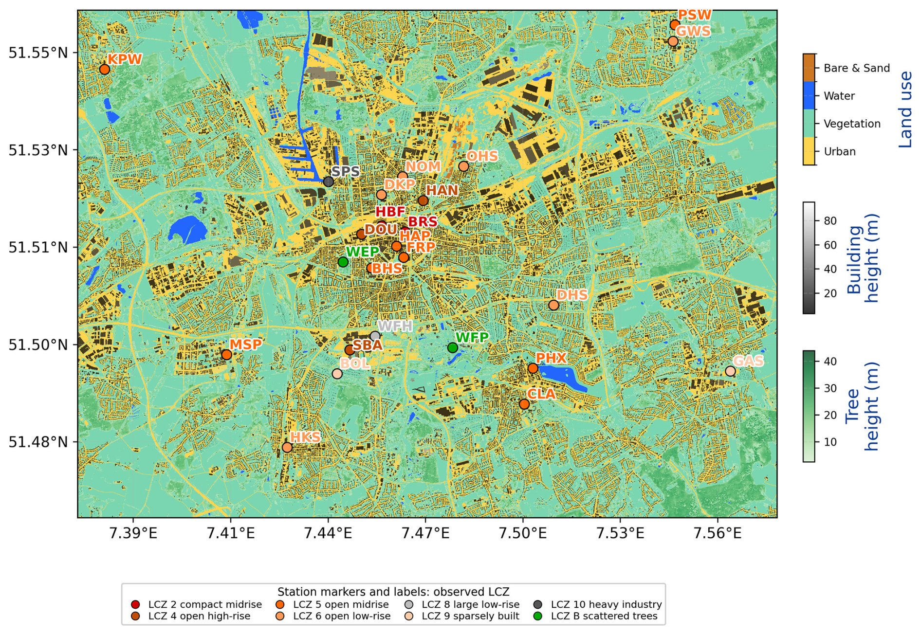
Figure 2 Dortmund model domain: land use, buildings, trees, and station points annotated with their respective ID on the common UTM32N grid. Generated during the input-build phase. Station markers and labels are colored according to the observed Local Climate Zone (LCZ) class reported in the station metadata, using the standard LCZ color scheme.

3 Results

We report computational performance and output volume for the Dortmund case study, illustrate the spatial imprint of the wind and UHI diagnostics, and evaluate station-based skill using aggregate statistics, distributions, and temporal and seasonal thermal stress metrics.

3.1 Computational performance

To quantify the practical impact of GPU acceleration, we benchmarked a single-day GLIDE-SOL run over Dortmund on a reduced 3129 × 3113 grid (2 m spacing). Using one NVIDIA A100 (40 GB) GPU, the 24 h simulation (saving UTCI, T_mrt, T_a, and V_10 m) completed in 254 s (10.6 s per simulated hour). The same configuration executed in CPU-only mode on the same node required 1285 s (53.5 s per simulated hour), corresponding to a wall-clock speed-up of about 5.1. For the GPU run, PyTorch CPU threading was restricted to num_threads=1 to avoid host-side oversubscription; in CPU-only mode all logical CPU threads were available.

In addition to compute acceleration, deferred repacking to LERC + ZSTD reduces I/O and storage requirements. For the Dortmund case-study grid, an uncompressed daily UTCI stack would occupy about 3.3 GB, whereas the repacked GeoTIFF is 251 MB (∼ 13 × smaller; 92 % reduction), using the compression error values described in Sect. 2.3.

3.2 Diagnostics of the wind and temperature corrections

The diagnostic wind module generates a directional attenuation coefficient field C(x,θ) that converts the domain-consistent 10 m wind to a morphology-dependent ventilation proxy. For θ=240° (south-westerly flow; Fig. 3), C is lowest within dense blocks, tree-covered areas, and leeward attenuation zones (C≪1), while major open corridors preserve higher effective wind speeds (C≈1). The yellow tree-height overlay helps identify areas where canopy sheltering contributes to locally low coefficients outside the densest building blocks. Values close to 1 should be interpreted as weak attenuation relative to the background wind rather than as explicit acceleration, because the model does not solve a mass-conserving flow field. Some smooth corridor-like structures in Fig. 3 therefore reflect the combination of overlapping attenuation zones, rotation back to the native grid, and Gaussian smoothing, and local anomalies around individual buildings or tree patches should be interpreted relative to the rasterized input geometry rather than as validated recirculation patterns. Although Reynolds-averaged and large-eddy CFD simulations provide higher-fidelity representations of shear layers and recirculation (Chu and Wang, 2025), the morphology-based C(x,θ) provides a computationally inexpensive surrogate that retains the main anisotropy imposed by urban form. This is the physical mechanism by which the Sol_WC_UHI configuration compensates for the lack of explicit urban drag in coarse meteorological forcing.

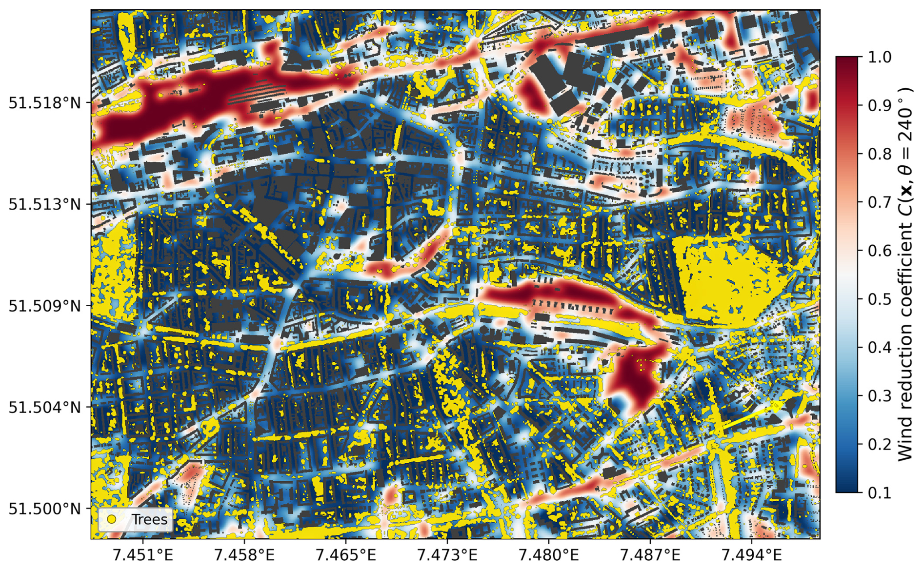
Figure 3 Example wind-reduction coefficient field C(x,θ) for θ=240° (south-westerly flow) over Dortmund. Dark-blue regions indicate strong wind attenuation in dense urban fabric, tree-covered areas, and leeward attenuation zones; warm colors highlight ventilation corridors with limited reduction. The yellow overlay labelled “Trees” marks positive tree-height pixels from the tree-height raster, with a dark halo added for readability, and the yellow arrow indicates the inflow direction used to compute the directional attenuation field.

The diagnostic UHI cycle acts on the background meteorological forcing rather than producing a standalone spatial field: it applies a night-time warming perturbation modulated by SVF and vegetation (Eq. 2). Its effect is therefore assessed through the station-based skill metrics and seasonal diagnostics presented below.

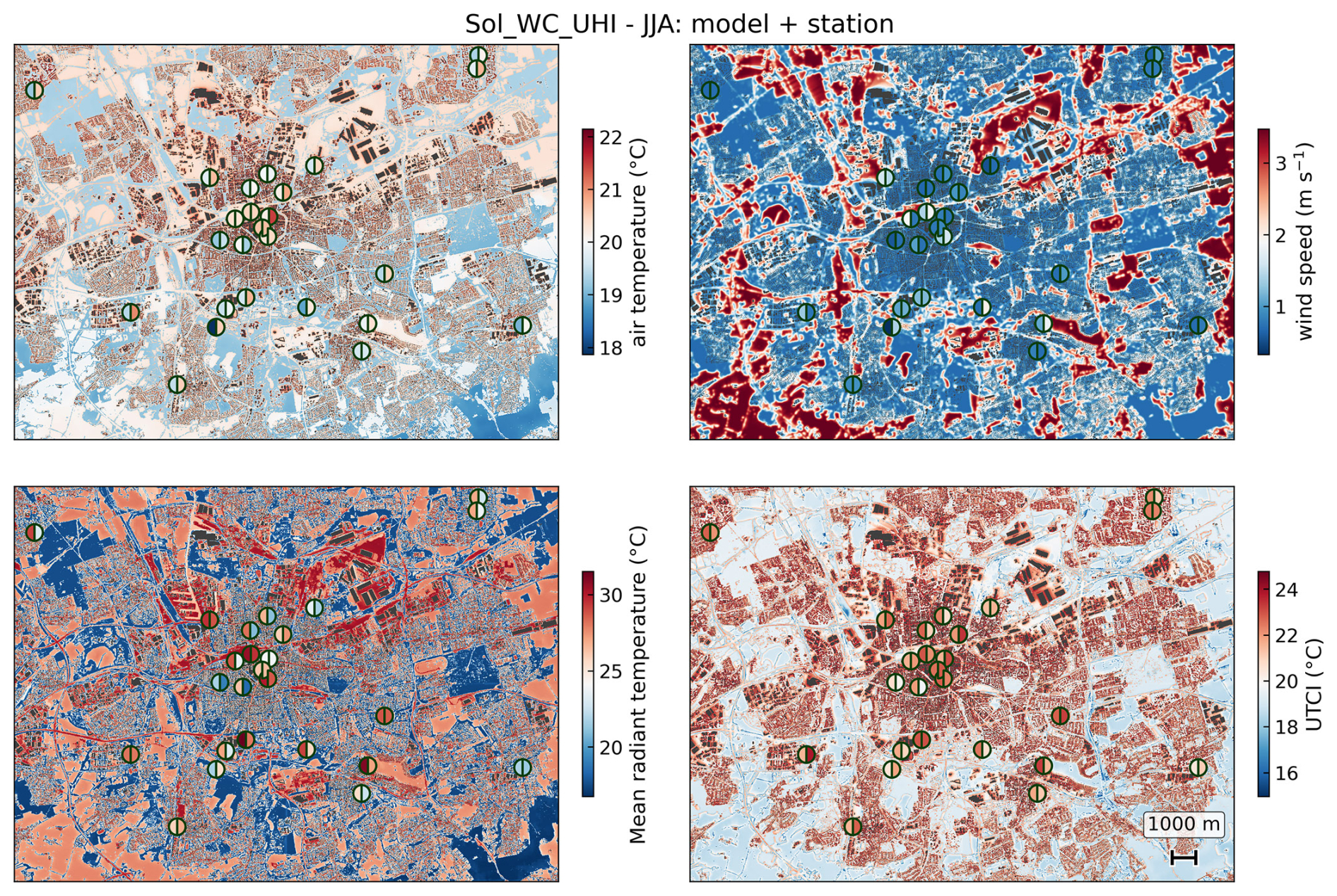
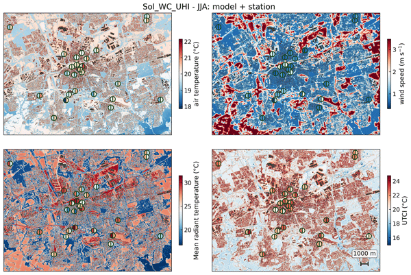
Figure 4 Summer (JJA) mean fields for the Sol_WC_UHI configuration. Panels show (top left) air temperature, (top right) wind speed, (bottom left) mean radiant temperature (T_mrt), and (bottom right) UTCI. Circles denote station locations; for each station, the left half of the symbol represents observed values, while the right half shows the corresponding modeled summer mean.

Figure 4 summarizes JJA mean fields from Sol_WC_UHI for central Dortmund. Station symbols report observed (left semicircle) and modeled (right semicircle) summer means at each location. Air temperature exhibits only modest spatial gradients and agrees well at station points. Wind speed shows strong morphology-driven heterogeneity, with low values in dense built-up areas and higher values in open corridors and peripheral zones; this pattern is consistent with the directional wind-reduction model and with the improved wind-speed statistics (Sect. 3.3). T_mrt displays pronounced small-scale variability due to shading and land cover, and the remaining differences at station locations are consistent with the residual T_mrt errors in Table 1. UTCI integrates these drivers and shows close agreement of summer means at station points, indicating that the diagnostic corrections translate into realistic warm-season thermal-stress levels.

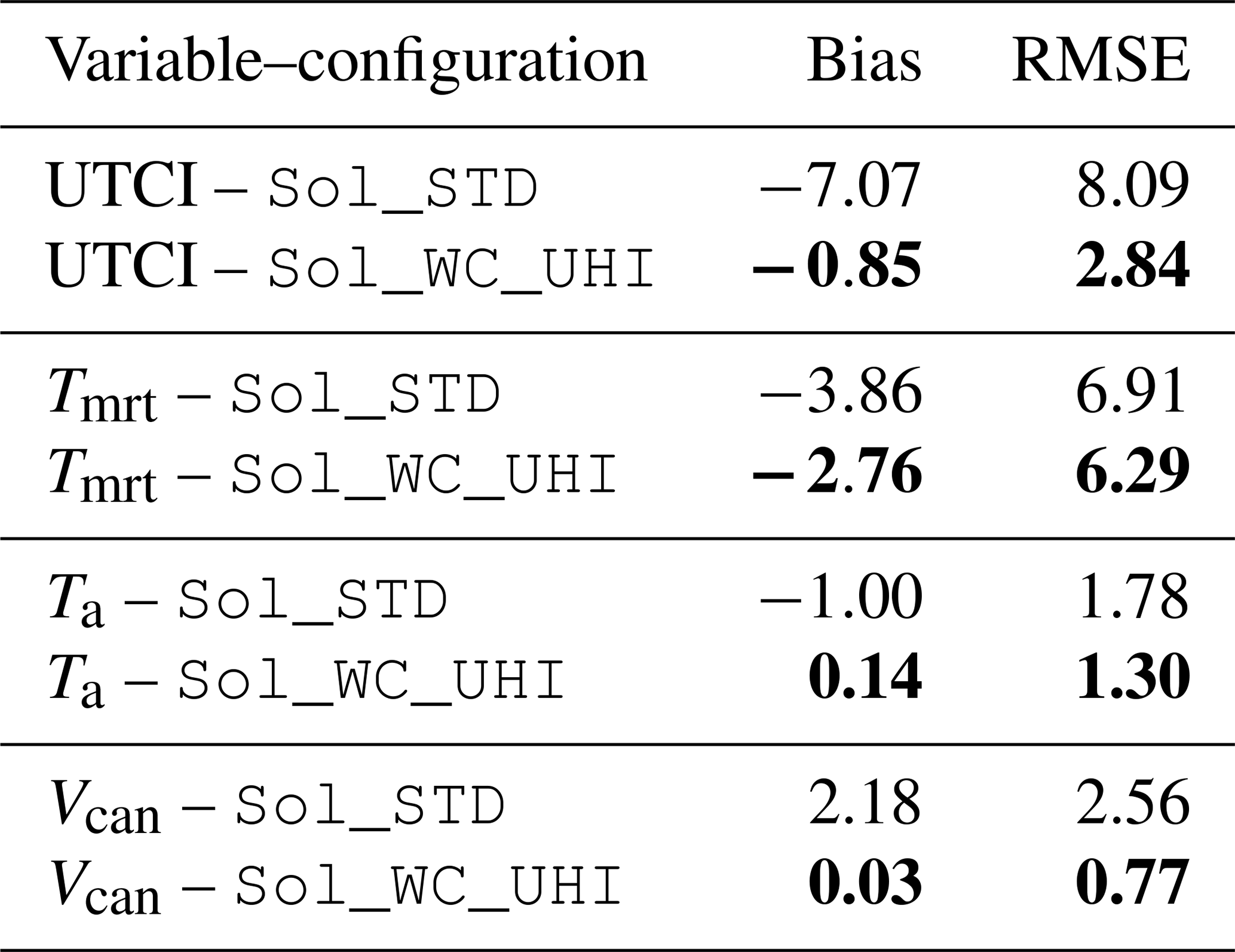
Table 1 Aggregate performance against observations. Bias and RMSE are in °C for UTCI/T_mrt/T_a and in m s⁻¹ for canopy wind speed V_can. Bold values indicate the best-performing configuration for each variable and metric.

3.3 Aggregate skill across all stations

Model skill is evaluated against hourly measurements from 25 stations with heterogeneous but overlapping temporal coverage between August 2024 and December 2025 (more than 250 000 station–hour records). We compare two configurations: a baseline run driven by unmodified ERA5 meteorology (Sol_STD) and a run that activates the morphology-based wind correction and the diagnostic UHI cycle (Sol_WC_UHI). Table 1 summarizes the aggregate performance against the station observations used in this paper. The combined corrections reduce the UTCI cold bias from −7.07 to −0.85 °C and cut RMSE from 8.09 to 2.84 °C (65 % reduction). Improvements are also evident for T_mrt (RMSE 6.91 °C → 6.29 °C) and canopy air temperature (RMSE 1.78 °C → 1.30 °C). The largest dynamical gain occurs for canopy wind speed V_can, where the strong positive bias in Sol_STD is largely removed (bias 2.18 → 0.03 m s⁻¹; RMSE 2.56 → 0.77 m s⁻¹).

The all-hour T_a statistics in Table 1 combine daytime and night-time conditions. This aggregation is useful for the overall UTCI evaluation, but it partly masks the mechanism of the diagnostic temperature correction: during daytime, T_a is affected primarily by ERA5 forcing and the elevation-based correction, whereas at night it is additionally affected by the UHI cycle.

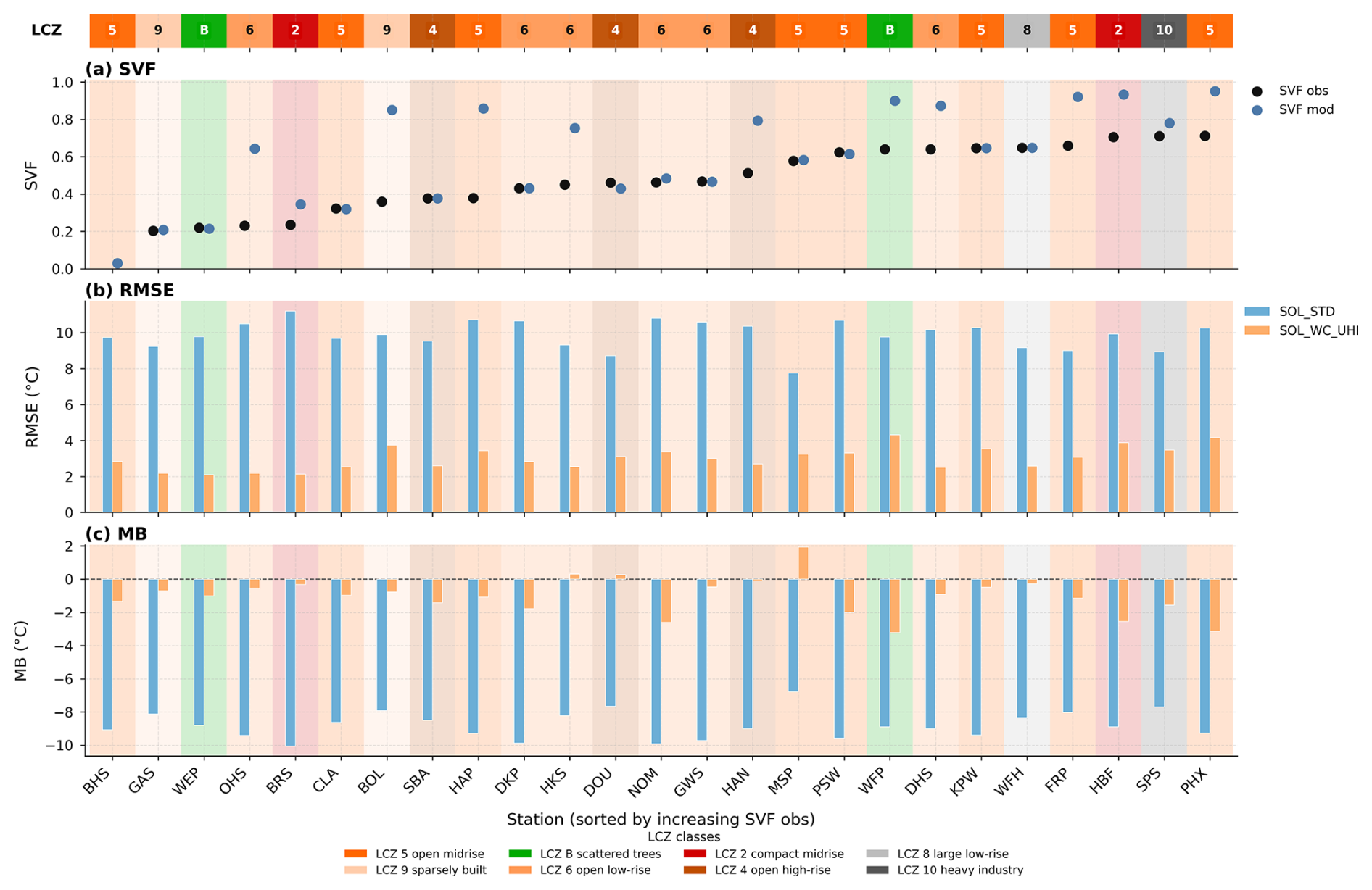
Figure 5 Station-level UTCI errors, sorted by observed SVF. Panels summarize RMSE and mean bias (MB) for Sol_STD and Sol_WC_UHI along the open-to-enclosed urban gradient; LCZ classes are shown as contextual descriptors of the observed station surroundings. Exact numeric values are reported in Appendix B.

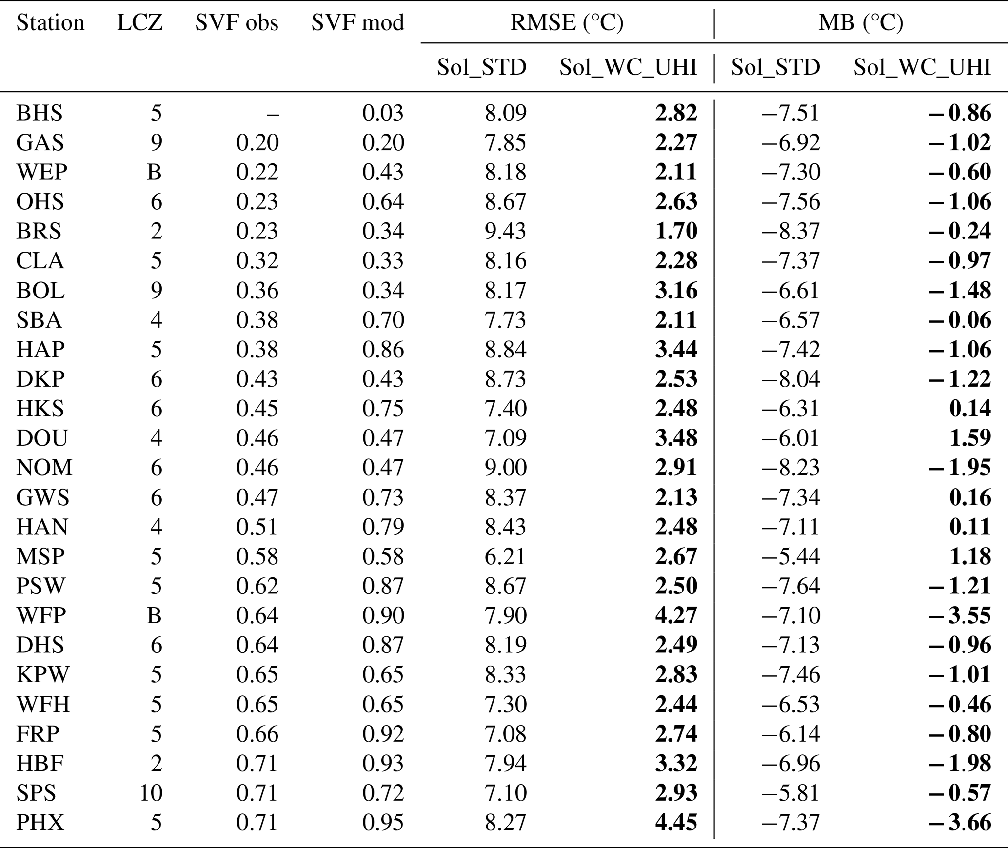
Figure 5 reports station-level UTCI errors (RMSE and mean bias, MB) for Sol_STD and Sol_WC_UHI, with sites sorted by sky-view factor (SVF) as a compact proxy for local enclosure and radiative exposure. The figure provides a first visual stratification along an open-to-enclosed urban gradient, while the exact numeric values are retained in Appendix B. Differences between observed and modeled SVF at individual stations mainly reflect representativeness: the model samples a 2 m grid cell from globally derived building and vegetation data, whereas the observed SVF characterizes the exact sensor surroundings, including small trees and facade details that are not always present in the input rasters. Open-source morphology datasets are also uncertain at this scale, especially for vegetation; discrepancies can therefore be larger in urban canyons with street trees or small vegetation elements where the local obstruction seen by the sensor differs from the rasterized building and vegetation layers. In Sol_STD, the mean bias is uniformly negative across the network (between −5.4 and −8.4°C) and RMSE remains high (6.2–9.4 °C) across the full SVF range, indicating that uncorrected forcing dominates the error (in particular, excessive wind cooling). With Sol_WC_UHI, RMSE decreases at every station (1.7–4.5 °C) and biases collapse towards zero (range −3.7 to 1.6 °C).

3.4 Scatter and distributional diagnostics

The scatter plots (Figs. 6 and 7) provide a compact view of systematic errors and conditional biases. For UTCI (Fig. 6), Sol_STD exhibits a pronounced cold bias, consistent with excessive convective cooling from overestimated winds and with missing nocturnal urban warming in the forcing. Activating wind attenuation and the UHI adjustment tightens the scatter and shifts the cloud towards the 1 : 1 line. In Fig. 7, the strongest improvement is in canopy wind speed V_can, where Sol_WC_UHI largely removes the positive bias. For canopy air temperature, the correction reduces both bias and RMSE, while T_mrt improves more modestly.

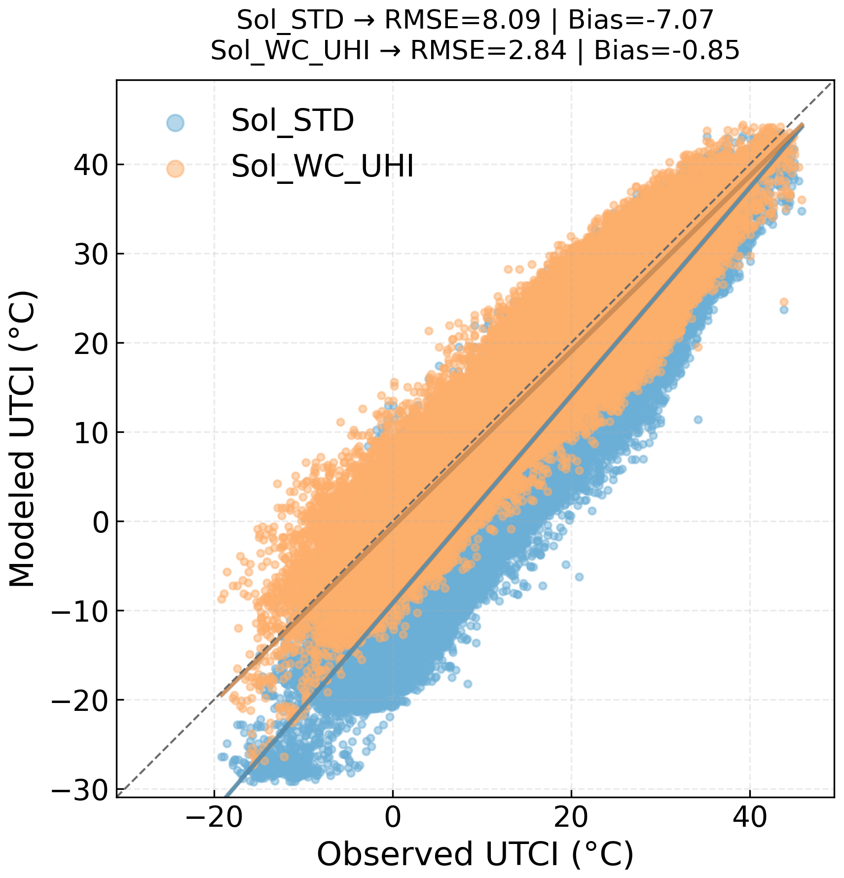
Figure 6 Observed vs. modeled UTCI for all stations and hours. The baseline Sol_STD shows a systematic cold bias, whereas Sol_WC_UHI concentrates closer to the 1 : 1 line, consistent with improved wind and temperature forcing.

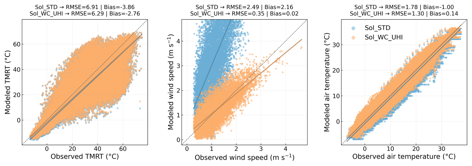
Figure 7 Observed vs. modeled (left) T_mrt, (center) canopy wind speed V_can, and (right) air temperature for all stations and hours. The baseline run (Sol_STD; labeled Sol_STD in the panel titles) shows large wind-speed overestimation and a cold bias in T_a, while the diagnostic wind and UHI corrections in Sol_WC_UHI reduce bias and RMSE, particularly for V_can.

The probability density functions (Fig. 8) provide a distribution-level evaluation of the main UTCI drivers and confirm that the corrections primarily act through wind and near-surface air temperature forcing.

For air temperature (top-left), both configurations reproduce the broad observed distribution, while Sol_WC_UHI shifts the PDF closer to the observations, consistent with the reduced T_a bias. The canopy wind speed V_can PDF (top-right) reveals the major deficiency of Sol_STD: a strong shift towards higher wind speeds and an unrealistically long high-wind tail (up to ∼ 10–12 m s⁻¹). Sol_WC_UHI largely removes this artifact, recovering the observed low-wind peak and damping the tail.

Consistently, the UTCI PDF (bottom-left) in Sol_STD is shifted towards lower values and exhibits an amplified cold tail, while Sol_WC_UHI moves the distribution back towards the observed mode and reduces the spurious cold tail. In contrast, T_mrt PDFs (bottom-right) show only limited sensitivity to the applied corrections, indicating that remaining errors are dominated by radiative forcing, surface properties, and input uncertainties rather than by aerodynamic exposure.

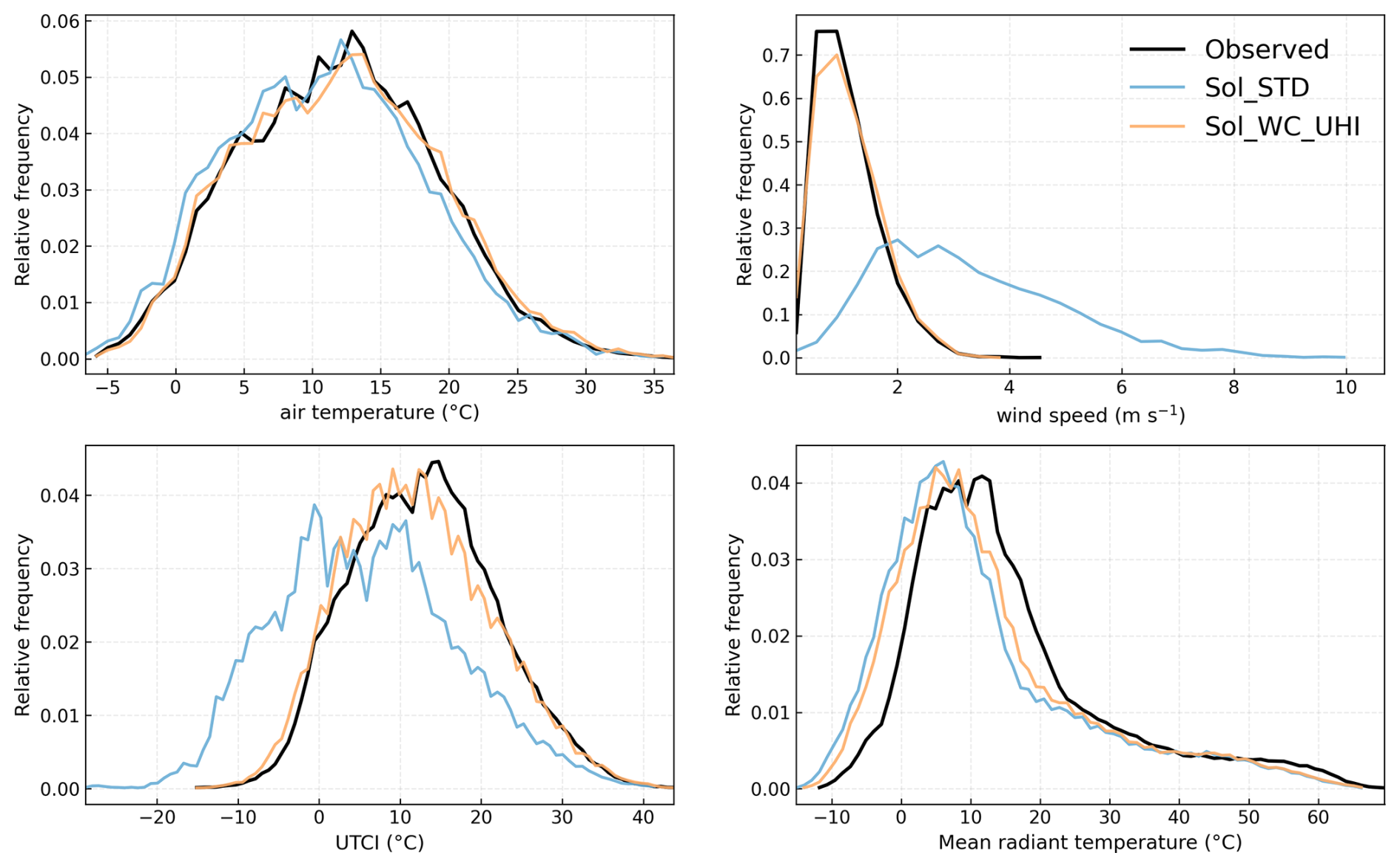
Figure 8 Probability density functions for canopy air temperature, canopy wind speed V_can, UTCI, and T_mrt. Model curves are compared with observations (black). The combined wind and UHI corrections in Sol_WC_UHI suppress the spurious high-wind tail and remove most of the UTCI cold shift present in Sol_STD.

3.5 Temporal behavior and thermal stress categories

To assess whether the improvements are persistent rather than limited to mean statistics, we examine the temporal evolution of spatially averaged conditions across all stations (Figs. 9 and 10) and the resulting UTCI category frequencies (Fig. 11). Because the series are aggregated over the entire station network, they primarily reflect synoptic-to-seasonal variability, so remaining offsets or amplitude errors indicate systematic bias.

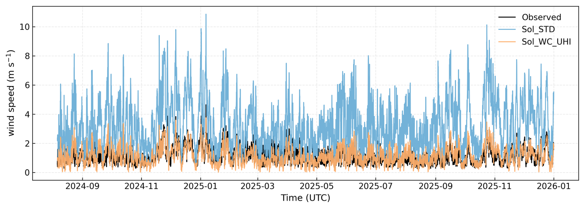
Figure 9 Time series of spatially averaged canopy wind speed V_can over all stations. The baseline Sol_STD shows frequent unrealistically high winds, whereas Sol_WC_UHI largely aligns with observed magnitudes after roughness rescaling and directional wind-reduction.

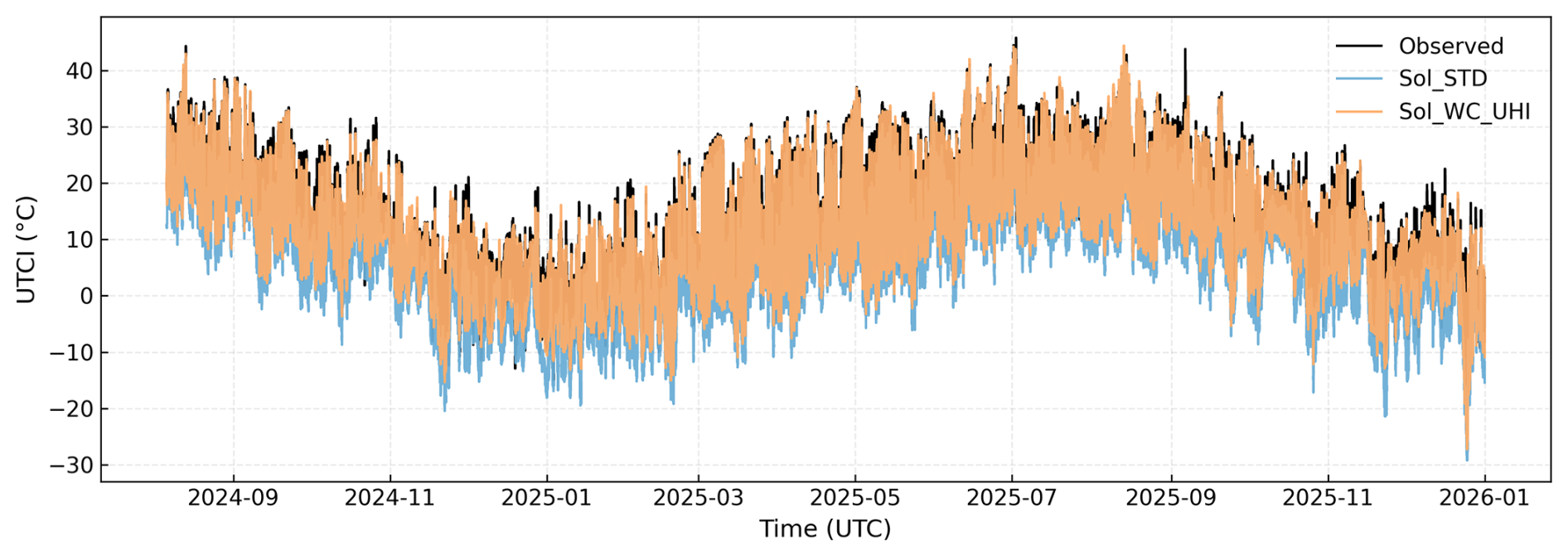
Figure 10 Time series of spatially averaged UTCI over all stations. Sol_STD remains systematically colder than observations, while Sol_WC_UHI reduces the offset and better reproduces the seasonal cycle and event-to-event variability.

The V_can time series (Fig. 9) highlights the dominant deficiency of the baseline configuration (Sol_STD, ERA5-driven winds without local urban diagnostics): winds are systematically too strong for the urban canopy and exhibit frequent high-wind excursions that are not present in the observations. In Sol_STD, wind speeds repeatedly spike above ∼ 8–12 m s⁻¹, whereas observed winds at the station network remain mostly below ∼ 2 m s⁻¹. The combined roughness rescaling and directional wind-reduction in Sol_WC_UHI suppress these excursions and constrain simulated winds to the observed envelope while preserving synoptic variability. This correction is critical because UTCI is highly sensitive to near-surface wind under cold and moderate conditions.

Consistent with the wind behavior, the UTCI time series (Fig. 10) shows a persistent cold bias in Sol_STD throughout the evaluation period, including exaggerated negative excursions during cold-season outbreaks and damped summer peaks. The corrected configuration Sol_WC_UHI substantially reduces this offset and reproduces the seasonal progression and much of the event-to-event variability. Periods of largest disagreement in Sol_STD coincide with intervals of excessive winds in Fig. 9, indicating that unrealistic aerodynamic exposure to ERA5 winds is a key driver of the baseline UTCI bias. The nocturnal UHI adjustment provides an additional contribution under stable night-time conditions.

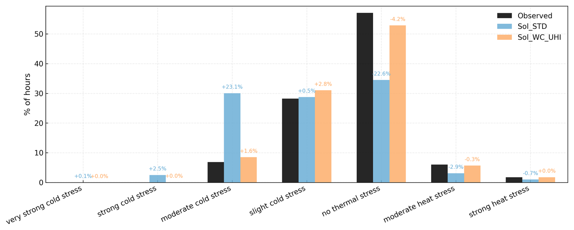
Figure 11 Hours per UTCI category across all stations. Bars show observed and simulated fractions; numbers above model bars indicate model–observation differences in percentage points. Sol_WC_UHI markedly improves the category distribution relative to Sol_STD, particularly by reducing spurious cold-stress frequencies and restoring the observed dominance of “no thermal stress”.

The improved continuous UTCI signal translates into a more realistic partitioning into thermal stress categories (Fig. 11). In the baseline case, the systematic cold shift redistributes hours from “no thermal stress” into cold-stress classes: Sol_STD overestimates moderate and strong cold stress by +23.1 and +2.5 percentage points, and underestimates “no thermal stress” by −22.5 percentage points. With Sol_WC_UHI, category biases are within a few percentage points across the spectrum (e.g., slight cold stress +2.8 percentage points, moderate cold stress +2.0 percentage points, and no thermal stress −4.6 percentage points), and warm-season heat stress frequencies align closely with the observations. Beyond station-based aggregation, the impact of the diagnostics is reflected in the spatial mapping of category frequencies across the Dortmund domain (Figs. 12 and 13), which determines where cold and heat stress exposure accumulates.

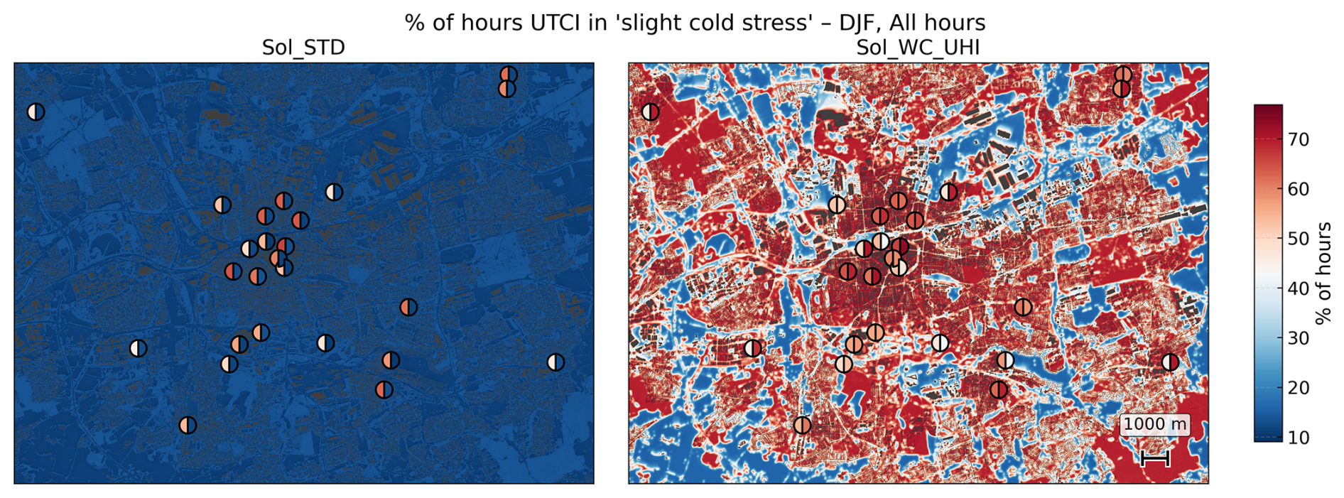
Figure 12 Fraction of hours classified as “slight cold stress” (UTCI) in DJF, considering all hours. Left: Sol_STD. Right: Sol_WC_UHI. Circles denote station locations; for each station, the left half of the symbol represents observed frequencies, while the right half shows the corresponding model value.

In winter (DJF), the fraction of hours in the “slight cold stress” category (0–9 °C UTCI) provides a sensitive diagnostic of the model's cold shift: if UTCI is systematically underestimated, hours are redistributed from this intermediate class into moderate and strong cold-stress categories. Figure 12 shows that Sol_STD assigns uniformly low fractions across the domain, masking the expected center-to-periphery contrast. With Sol_WC_UHI, a clear urban-core signal emerges, with higher slight-cold frequencies over dense city fabric and lower values over parks, open areas, and the peri-urban fringe where ventilation is stronger. Station symbols reinforce this pattern, with inner-city sites moving toward observed frequencies while peripheral sites retain lower fractions.

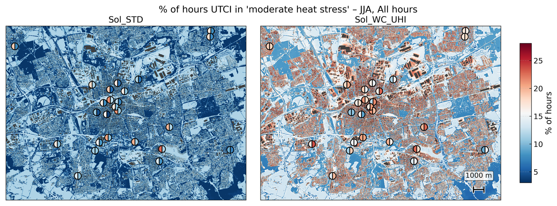
Figure 13 Fraction of hours classified as “moderate heat stress” (UTCI) in JJA, considering all hours. Left: Sol_STD. Right: Sol_WC_UHI. Circles denote station locations; for each station, the left half of the symbol represents observed frequencies, while the right half shows the corresponding model value.

In summer (JJA), “moderate heat stress” (26–32 °C UTCI) shows a strong spatial contrast tied to urban form and ventilation (Fig. 13). In Sol_STD, moderate heat-stress frequencies are muted and relatively flat, consistent with the tendency to damp warm-season stress through excessive wind speeds even in dense neighborhoods. With Sol_WC_UHI, a center-to-outskirts gradient becomes visible: higher fractions emerge over compact, wind-sheltered urban fabric and heavily built corridors, while parks, green areas, and the outer suburban fringe retain low values. Station symbols indicate that the corrected configuration better captures both the elevated inner-city frequencies and the lower peripheral values without overstating the overall occurrence.

4 Discussion

The Dortmund evaluation demonstrates that two lightweight diagnostics – directional wind attenuation and a nocturnal UHI adjustment – substantially reduce the cold bias that arises when SOLWEIG is forced directly with coarse reanalysis fields. In the baseline configuration (Sol_STD), near-surface winds are too strong for the urban canopy and night-time air temperature is underestimated, producing a persistent cold offset and an exaggerated cold tail in UTCI (Figs. 10 and 8). The temporal and category analyses indicate that the corrections improve not only mean skill but also event-scale variability and the partitioning of hours into cold- and heat-stress classes, which is essential for exposure assessments. Because the workflow is driven by globally available inputs and standardized preprocessing, these gains are achieved without bespoke local data assembly, supporting consistent multi-city applications.

The wind diagnostic is the dominant contributor to the UTCI improvement. By imprinting building and tree morphology onto the canopy wind through the coefficient fields C(x,θ) (Fig. 3), Sol_WC_UHI removes the spurious high-wind tail (Fig. 8) and nearly eliminates the wind-speed bias (Table 1), consistent with Röckle-style conceptualizations of urban flow (Röckle, 1990). The resulting spatial gradients align with dense urban cores and more ventilated outskirts, reinforcing the physical consistency of the approach. The remaining station-to-station spread suggests that unresolved local exposure and representativeness (e.g., site-specific shielding) still matter, but to a much lesser extent than the forcing bias.

The diagnostic UHI cycle provides a complementary correction that is most relevant under stable nocturnal conditions, particularly in winter. It shifts the distributions of air temperature and UTCI towards the observations and reduces extreme cold-stress episodes (Figs. 8 and 10). Its simple structure keeps computational cost low and enables consistent application across regions, but the residual positive T_a bias in Sol_WC_UHI (Table 1) indicates that a single diagnostic parameter set cannot capture the full range of synoptic regimes and advective effects. The local vegetation term in the present UHI parameterization is another simplification, and future versions should replace it with a stability-aware neighborhood representation of vegetation cooling. Wind is the dominant contributor to the all-hour UTCI improvement, while future work should further improve the reproduction of air temperature.

T_mrt improvements are comparatively modest (Table 1; Figs. 7 and 8), consistent with T_mrt being driven primarily by radiative forcing and urban geometry. Because the Dortmund simulations use the SOLWEIG v2022a anisotropic diffuse-shortwave and longwave sky schemes (Wallenberg et al., 2020, 2023), the remaining T_mrt bias cannot be attributed simply to an omitted isotropic-sky approximation. Air temperature (T_a) influences T_mrt mostly indirectly: it modulates atmospheric longwave emission (through sky emissivity) and, in SOLWEIG, it is used to parameterize surrounding surface temperatures, including wall temperature (T_wall), which in turn affects the longwave radiation received by the pedestrian. Remaining discrepancies likely reflect uncertainties in morphology and surface properties and missing processes such as anthropogenic heat and its effect on surface temperatures and long-wave emission, especially during the heating season (Liu et al., 2023; Wallenberg et al., 2026). In a global context, improving canopy and surface characterization layers is therefore a key path to further gains in radiative skill.

The T_mrt observations should also be interpreted in the context of the measurement setup. In the Dortmund network, T_mrt is derived from black-globe temperature and accompanying meteorological measurements following International Electrotechnical Commission (2021) using Decentlab DL-BLG sensors. These observations were not calibrated in this study against 3-D net radiometers, so no calibration-based adjustment was applied before model evaluation.

From a modeling and reproducibility standpoint, GLIDE-SOL addresses scalability constraints that often limit city-scale, meter-scale applications. GPU acceleration reduces wall-clock time by about a factor of five for the Dortmund benchmark. Deferred LERC + ZSTD repacking reduces output volumes by about 92 % while enforcing explicit error budgets per variable, producing lightweight GeoTIFF archives that reduce I/O and storage pressure. Together with the global input pipeline, these features enable multi-year, city-scale UTCI mapping without prohibitive compute or storage requirements and make coordinated multi-city experiments operationally feasible.

Limitations of the present demonstration include uncertainty in open building and tree-height products, a simplified diagnostic representation of urban heat storage, and reliance on coarse ERA5 forcing that omits mesoscale circulations and city-wide advection (Kittner et al., 2025). Additional limitations are the absence of an urban modification to relative humidity, the lack of anthropogenic heat contributions from building heating/cooling and traffic, and the use of a simplified urban wind-reduction model that cannot fully capture local channeling or sheltering, does not enforce mass conservation, and does not include terrain-following wind coordinates. Several numerical choices in the current wind implementation – including the number of wind sectors, the wake-length multipliers, and the Gaussian smoothing length – were selected pragmatically for robustness and computational efficiency rather than calibrated independently. Future versions should introduce a stability-dependent representation of intra-urban UHI variability, because the physically relevant blending scale depends on atmospheric stability, turbulence, and advection, as shown experimentally for urban green-space cooling by Haeffelin et al. (2024). Stability-dependent spatial smoothing or neighborhood-scale vegetation metrics remain important sensitivity tests. Future work should therefore evaluate the diagnostics across multiple cities and climates, quantify sensitivity to morphology and roughness assumptions, test alternative directional and smoothing settings, perform component-ablation experiments for wind, elevation, and UHI corrections, and explore coupling the UHI signal to mesoscale predictors, modeled radiation and wind, urban canopy schemes, or terrain-aware diagnostic wind formulations such as terrain-following QUIC-URB/QUIC-Fire coordinate systems (Robinson et al., 2023), with attention to regional variability in global input quality.

5 Conclusions

GLIDE-SOL extends SOLWEIG into a scripted, globally deployable workflow that (i) builds the full set of SOLWEIG inputs from global data sources with standardized preprocessing, (ii) adds computationally cheap diagnostics to mitigate known biases in coarse meteorological forcing over cities, and (iii) enables scalable simulations through GPU acceleration and bounded-error output compression that yields lightweight GeoTIFF archives for long-term analyses. The automated data-engine and configuration-driven pipeline are key novelties that make city-scale UTCI mapping reproducible and transferable without bespoke local datasets.

For Dortmund (25 stations; more than 250 000 station–hour records), the enhanced configuration Sol_WC_UHI reduces UTCI RMSE from 8.09 to 2.84 °C and the mean bias from −7.07 to −0.85°C. The improvement is driven primarily by correcting the wind speed (bias 2.18 → 0.03 m s⁻¹), with additional gains from the nocturnal UHI adjustment. Beyond mean skill, the corrections restore the temporal evolution of UTCI, reduce spurious cold-stress hours, and recover realistic spatial contrasts in winter cold stress and summer heat-stress hotspots, indicating that globally driven diagnostics can reproduce both temporal and spatial exposure signatures.

On the technical side, a 24 h benchmark on a 3129 × 3113 grid completes in 254 s on a single NVIDIA A100 GPU (about 5× faster than CPU-only), and daily outputs can be reduced by over 90 % using LERC + ZSTD with explicit error budgets. The combination of fast GPU execution and lightweight GeoTIFF storage supports routine, meter-resolution UTCI mapping at city scale over multi-year periods, enabling consistent multi-city benchmarking, scenario testing, and evaluation of heat-mitigation strategies at regional to global scales.

Appendix A: Wind-model comparison

Table A1 Comparison between the diagnostic wind treatment implemented in GLIDE-SOL and the full Röckle/URock methodology.

Appendix B: Station-level UTCI errors

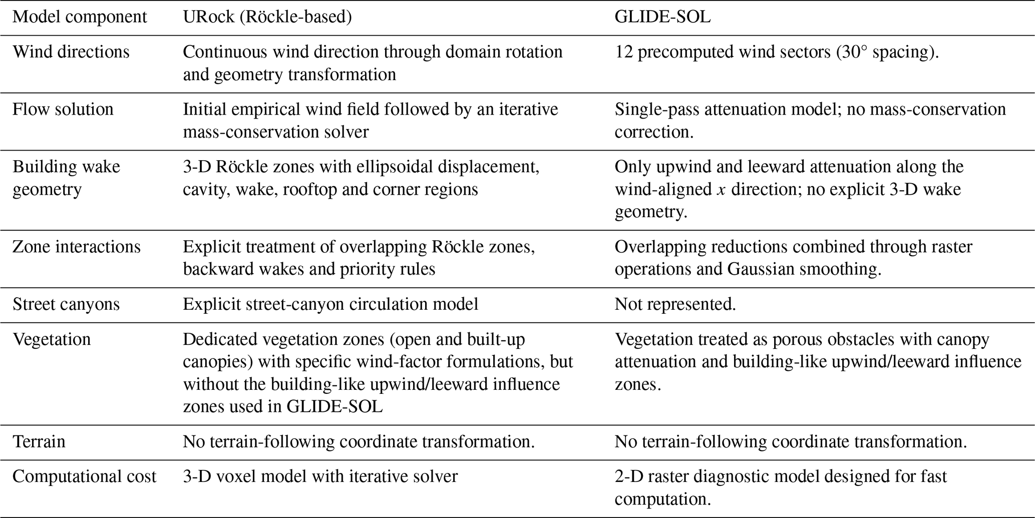
Table B1 UTCI errors by station (sorted by SVF obs). LCZ classes are taken from the field-based station metadata and are reported here as contextual descriptors of the observed station surroundings. Bold indicates lowest error for each station and metric.