Design and implementation of a Newtonian relaxation scheme in the NOAA GFDL Sea Ice Model (SIS2)

Regional sea ice models often do not cover the full extent of polar ice and instead include open ocean boundaries that are not ice-free year-round. This necessitates the specification of lateral boundary conditions for sea ice, an inherently challenging task for most sea ice models. Although this issue is less critical for pan-polar domains, the interior ice state still needs to be constrained for many applications. In this study, we present the design and evaluation of a Newtonian relaxation algorithm for sea ice, implemented in the NOAA Geophysical Fluid Dynamics Laboratory (GFDL) Sea Ice Simulator (SIS2). The algorithm can be applied both at the lateral boundaries to impose open boundary conditions and within the interior domain to constrain sea ice thickness and concentration toward prescribed target fields. The method is flexible and can be applied anywhere in the domain, making it especially well-suited for regional applications of sea ice models with variable ice cover along their boundaries. The method is evaluated within a regional forecasting system based on the NOAA GFDL ocean model (MOM6) coupled with sea ice model (SIS2) for two regional configurations: the Northeast Pacific and the Arctic Ocean. Sensitivity experiments spanning a range of relaxation time scales and nudging strengths demonstrate that the method substantially improves the representation of sea ice and associated ocean surface fields, offering a practical solution for both boundary and interior constraints in regional sea ice modeling.

1 Introduction

Regional applications of sea ice models are often challenged by two closely related issues: the specification of appropriate lateral open boundary conditions (LBCs) and the need to constrain the interior ice state. The former is less problematic when the lateral boundaries lie within ice-free ocean regions, but becomes critical when lateral boundaries intersect areas of variable ice cover. In such scenarios, the model solution depends critically on specification of LBCs for sea ice state variables. Even for domains with well-defined LBCs, constraining the interior ice state is essential for applications such as forecasting and reanalysis, where errors in initial or boundary conditions can propagate throughout the domain.

Application of LBCs in sea ice models remains an area of active research, with limited detailed information available in the scientific literature. Most regional applications rely on a combination of relaxation and radiation schemes, or on prescribed Dirichlet or Neumann boundary conditions (Smedsrud et al., 2006; Lemieux et al., 2008; Hunke et al., 2015; Rousset et al., 2015; Duarte et al., 2022). For example, Rousset et al. (2015) implemented a flow relaxation scheme in the Louvain-La-Neuve sea ice model (LIM3.6), in which ice state variables are relaxed toward interior or external values depending on flow direction. Similarly, the Los Alamos Sea Ice CodE (CICE5; Hunke et al., 2015) supports time-varying LBCs through relaxation toward prescribed values in halo cells and adjacent interior grid cells (Duarte et al., 2022).

While these methods are comparatively straightforward to implement, the development of more advanced open boundary condition schemes remains challenging because of both numerical and physical considerations. Sea ice fields often exhibit sharp spatial gradients, which are physically consistent with the underlying dynamics, thermodynamics, and ocean-atmosphere forcing. Moreover, the presence of sea ice rheology implies that LBCs must be dynamically consistent with the internal ice stress field, whose influence can extend far into the interior of the ice pack. However, if LBCs introduce discontinuities that are not dynamically balanced with the interior ice momentum or internal stress fields, they can lead to unrealistic or unstable model behavior. In addition, mismatches between inflowing sea ice properties and the local oceanic or atmospheric conditions may result in excessive melting and unphysical freshwater input along the boundary. In practice, only a limited set of sea ice variables is often available for specifying boundary conditions, making it difficult to prescribe a fully dynamically consistent sea ice state at the boundaries. These challenges motivate approaches that not only prescribe boundary conditions but also constrain the interior solution to reduce sensitivity to boundary errors.

When lateral boundaries are close to the forecast region, boundary-imposed signals can penetrate the interior. As a result, biases and errors in the LBCs may propagate inward and corrupt the interior solution (Nicolis, 2007). One strategy to mitigate this effect is to extend relaxation beyond the boundaries and nudge the interior ice state toward prescribed target fields (Lindsay and Zhang, 2006). Relaxation is commonly employed to improve sea ice initial conditions through the gradual assimilation of observational data into the model fields.

Although advanced data assimilation techniques for sea ice are available (e.g., Fritzner et al., 2019), relaxation-based nudging provides a practical, computationally efficient, and robust alternative for regional modeling applications (Tietsche et al., 2013; Hunke et al., 2015; Prasad et al., 2021). Simple direct nudging approaches have been shown to effectively constrain ice fields (Audette and Kushner, 2022). The classical Newtonian relaxation method discussed here falls into the category of “direct sea ice nudging” (Smith et al., 2017).

This paper presents the design and implementation of sea ice relaxation in the Geophysical Fluid Dynamics Laboratory (GFDL) Sea Ice Simulator version 2 (SIS2; Adcroft et al., 2019). The development is motivated by the increasing application of SIS2 to regional polar and subpolar domains, where realistic LBCs and interior constraints are essential. The primary objective of the developed relaxation algorithm is to improve sea ice initial conditions for high-latitude marine forecasts, thereby enhancing prediction skill on short-term to seasonal time scales (Dirkson et al., 2019), without precluding the development of more sophisticated sea-ice initialization approaches in future forecast systems.

The primary goals of this study are to evaluate the performance of the implemented sea ice relaxation approach and to assess its impact on sea ice and ocean surface fields. The methodology is outlined and the algorithm is evaluated within the coupled SIS2 modeling framework in two regional applications: the Northeast Pacific and the Arctic Ocean. These domains differ in their sensitivity to lateral boundary conditions and interior constraints. Together, these applications provide a complementary assessment of the effectiveness of relaxation for both boundary forcing and interior state correction.

2 Northeast Pacific and Arctic Ocean regional configurations

Performance and testing of the ice relaxation algorithm is demonstrated with two regional forecasting systems set up for the Northeast Pacific (NEP10k) region (Fig. 1a) and the Arctic Ocean (ARC10k, Fig. 1b). Both systems employ the GFDL ocean model MOM6 and sea ice model SIS2 (Adcroft et al., 2019), coupled with Carbon, Ocean Biogeochemistry and Lower Trophics biogeochemical model (COBALTv3) (Stock et al., 2025). The ocean model parameters used in the two configurations are largely similar, whereas the sea ice parameters have several differences, as discussed in the following sections. Descriptions of the model components are provided in Adcroft et al. (2019), with configuration details for regional MOM6 applications documented in Ross et al. (2023) and Drenkard et al. (2025). Here we summarize the key configuration details and physical parameters of the ocean model used in the numerical experiments.

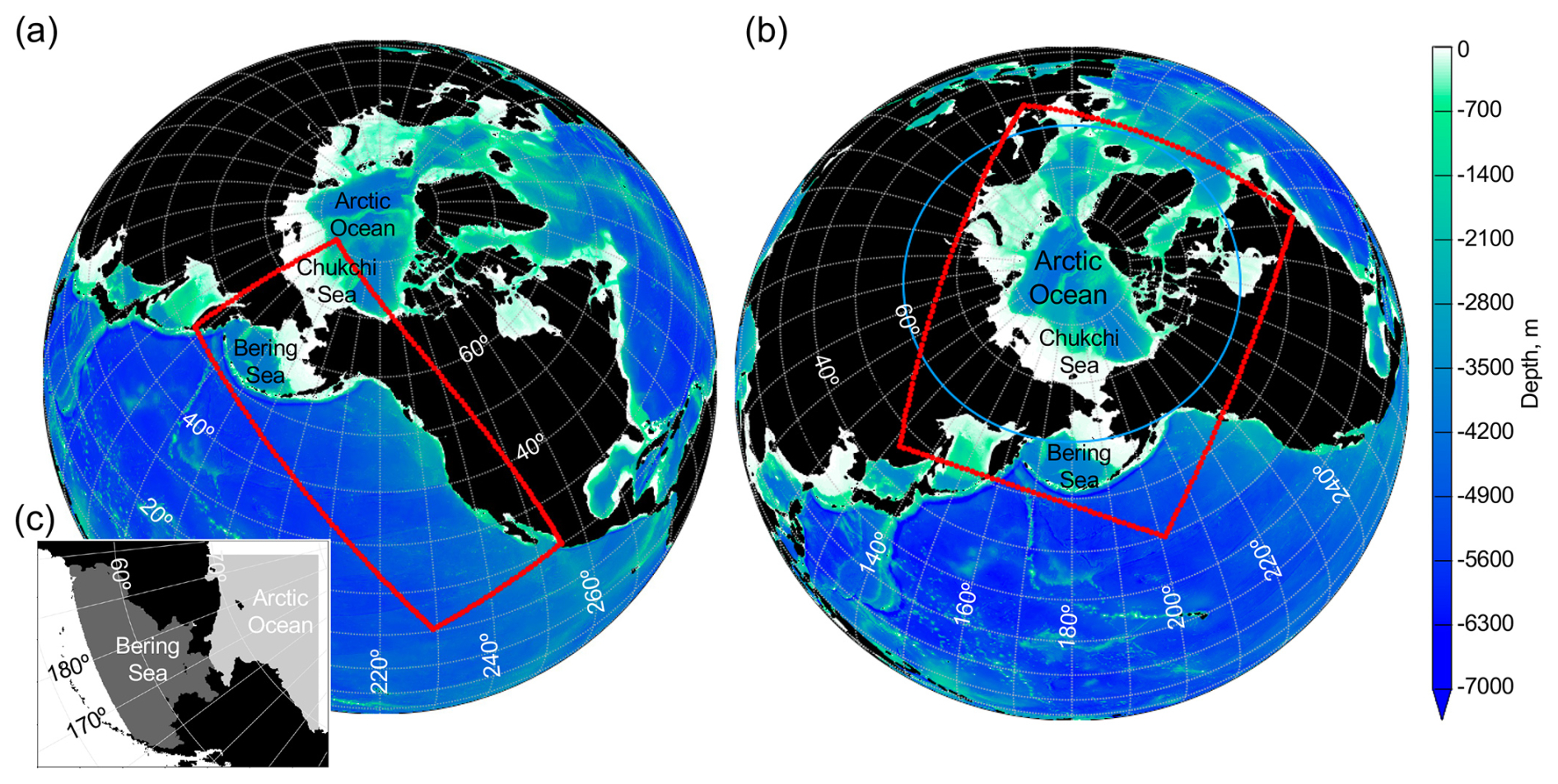
Figure 1 Computational domains. (a) Bottom topography and the Northeast Pacific (NEP10k) domain. The red box delineates the domain boundaries. (b) Bottom topography and the Arctic Ocean (ARC10k) domain, also outlined in red. The 60° N latitude, shown in blue, marks the boundary of the relaxation zone used in the ARC10k experiments discussed in the text. (c) The northern portion of the NEP10k domain. Shaded regions indicate areas used for validation in the NEP10k experiments. For the ARC10k domain, validation is performed within the relaxation region located north of 60° N.

2.1 Modeling domains

The NEP10k domain follows the western coast of North America, extending from the tropical Pacific to the Bering and Chukchi Seas (Fig. 1a). The computational grid is an orthogonal curvilinear Arakawa C grid with spatially varying horizontal resolution of approximately $\mathrm{1}/\mathrm{12}$°, yielding nearly homogenous 10 km spacing over the region of interest.

The study focuses on the northern portion of the NEP10k domain encompassing the Bering and Chukchi Seas (Fig. 1c), which exhibit contrasting sensitivities to LBCs. In the Bering Sea, sea ice primarily forms over the continental shelf during winter with minimal advection from the Arctic Ocean (Wang et al., 2009), implying weak sensitivity to LBCs. In contrast, ice conditions in the Chukchi Sea are strongly influenced by oceanic heat flux through the Bering Strait and by ice advection from the Arctic Ocean (Serreze et al., 2016), making this region more sensitive to prescribed LBCs.

ARC10k covers the Arctic and subarctic regions (Fig. 1b) and employs a horizontal grid spacing of approximately $\mathrm{1}/\mathrm{12}$° (∼ 10 km). In this configuration, most ice-covered regions are far removed from the lateral boundaries, such that the influence of LBCs on the interior solution is expected to be minimal. Instead, the primary challenge is constraining the interior sea ice state. Given well-documented model biases in Arctic sea ice thickness, concentration, and drift (Johnson et al., 2012; Schweiger and Zhang, 2015; Bouchat et al., 2022; Hutter et al., 2022; Frankignoul et al., 2024), particularly in the marginal ice zone (MIZ; Fritzner et al., 2019; Dumont, 2022), ARC10k serves as a useful testbed for evaluating the effectiveness of interior relaxation in improving simulated ice conditions.

2.2 Physical ocean model

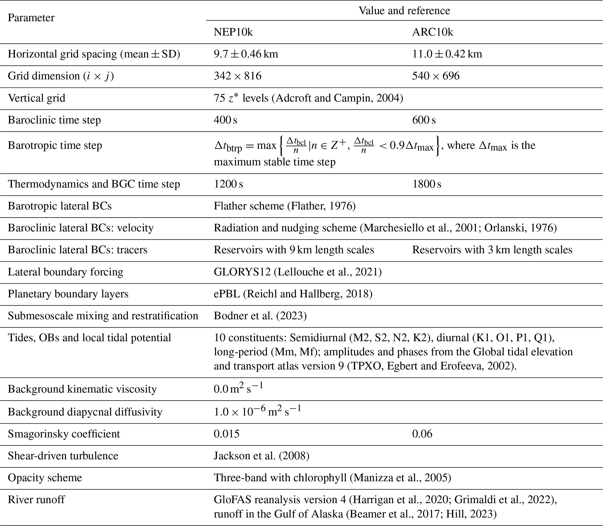
The main configuration choices used in the physical ocean model (MOM6) follow those described in Ross et al. (2023) and Drenkard et al. (2025). Key MOM6 parameters for both configurations are summarized in Table 1. These particular MOM6 configurations employ a z^* vertical coordinate system (Adcroft and Campin, 2004) with partial bottom cells and 75 vertical layers, offering fine resolution (∼ 2 m) in the upper 30 m, gradually increasing to 250 m in the deep ocean, similar to the setup in Adcroft et al. (2019). The model employs split-explicit time stepping (Hallberg and Adcroft, 2009; Griffies et al., 2020), with a baroclinic time step, Δt_bcl, and a time-varying barotropic time step, Δt_btrp, whose values are summarized in Table 1. Thermodynamics and biogeochemistry are updated at a time step of 1200 s.

Table 1 Major parameters used in the physical ocean component (MOM6).

The simulations include tidal forcing, imposed both at the lateral boundaries and through the astronomical tidal potential. The choice of lateral boundary conditions is consistent with Ross et al. (2023). Ocean lateral boundary conditions are derived from the Copernicus Global $\mathrm{1}/\mathrm{12}$° Oceanic and Sea Ice Reanalysis (GLORYS12; Lellouche et al., 2021). Atmospheric forcing fields (momentum, heat, precipitation, and radiation fluxes) are derived from the hourly European Centre for Medium-Range Weather Forecasts (ECMWF) Reanalysis 5 (ERA5; Hersbach et al., 2020).

2.3 Sea ice model

The main characteristics of the sea ice model SIS2 are summarized in Table 2. SIS2 employs a horizontal C-grid collocated with the ocean grid and simulates the evolution of the ice thickness distribution through ice dynamics, thermodynamic growth and melt, and mechanical redistribution. Ice column thermodynamics follow Bitz and Lipscomb (1999), and shortwave radiative transfer is based on Briegleb and Light (2007), as implemented in CICE version 4.1 (Hunke and Lipscomb, 2010). Mechanical redistribution due to ridging is represented using a standard redistribution scheme (Rothrock, 1975; Thorndike et al., 1975; Hibler, 1980), and ice rheology is described by the elastic–viscous–plastic (EVP) formulation (Bouillon et al., 2009).

Table 2 Major parameters used in the sea ice component (SIS2).

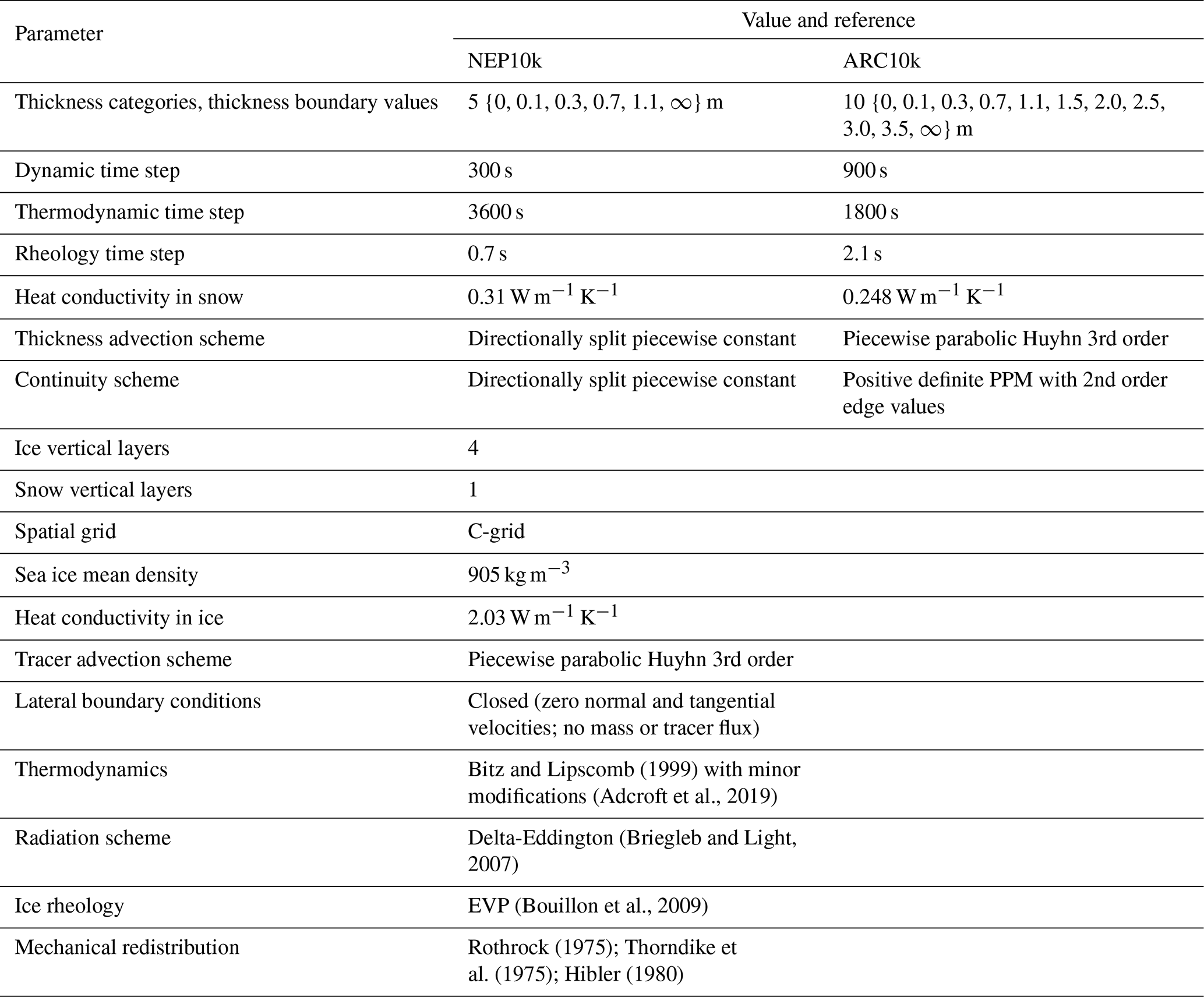
Sea ice is partitioned into a specified number of thickness categories (N_c). Five ice thickness categories in NEP10k are chosen to provide better resolution for thin ice. In ARC10k, ice is partitioned into 10 ice categories offering a sufficiently fine representation of the range of ice thicknesses in the Arctic. For each thickness category, sea ice has 4 vertical layers (N_i) and 1 snow layer (N_s). In both configurations, the sea ice lateral boundaries are closed. In SIS2, closed boundaries are modeled as land points where the normal component of ice velocity is constrained to zero, and a no-slip condition is applied to the tangential component of the ice velocity. Ice stress at these boundaries is treated implicitly, naturally vanishing and ensuring zero flux across the land or closed boundary faces. The dynamic and thermodynamic processes are time-split, with dynamics integrated using a shorter dynamic time step, followed by thermodynamic updates applied at a longer thermodynamic time step.

3 Validation methodology and relaxation target fields

3.1 Sea ice data used for nudging

The sea ice relaxation algorithm nudges ice concentration and thickness toward prescribed target values. Although the algorithm does not require these two fields to be physically consistent, its performance improves when they are aligned. For the gridded products considered, target fields for sea ice concentration and thickness can be derived from satellite derived estimates and sea ice reanalysis products. Satellite observations provide broad coverage of sea ice concentration, but the use of satellite-derived ice thickness for nudging remains challenging due to limited temporal coverage, data gaps, retrieval uncertainties, and seasonal biases, particularly during melt conditions (e.g., Laxon et al., 2013; Labe et al., 2018; Tilling et al., 2018). In addition, inconsistencies between independently derived concentration and thickness products may introduce unphysical behavior during relaxation (Zygmuntowska et al., 2014).

In this study, sea ice concentration and thickness are relaxed toward fields from version 2.1 of the Pan-Arctic Ice Ocean Modeling and Assimilation System (PIOMAS) reanalysis. PIOMAS is a coupled data-assimilative modeling system that includes a multicategory thickness and enthalpy distribution (TED) sea ice model (Zhang and Rothrock, 2001, 2003) and the Parallel Ocean Program (POP) ocean model (Smith et al., 1992). The model spans the pan-Arctic region with open boundaries at 45° N and has a spatial resolution of 22 km. Atmospheric forcing (surface wind, surface air temperature, cloud cover) is derived from the NCEP/NCAR Reanalysis 1 (Kalnay et al., 1996).

PIOMAS assimilates sea ice concentration from the NSIDC Near-Real-Time product and sea ice velocity (Lindsay and Zhang, 2006), but does not assimilate sea ice thickness. Despite this limitation, previous studies have shown that PIOMAS reproduces observed patterns of sea ice thickness, volume, and motion with reasonable fidelity (Schweiger et al., 2011; Stroeve et al., 2014; Wang et al., 2016; Labe et al., 2018; Petty et al., 2022; Schweiger and Zhang, 2015).

Although PIOMAS fields are used as the target state in the experiments presented here, the relaxation methodology is general and has been successfully applied using other target datasets, including GLORYS sea ice fields, as well as synthetic test fields during the development and verification phase. The choice of PIOMAS does not affect the formulation of the relaxation algorithm.

3.2 Model performance evaluation metrics

The effectiveness of the relaxation algorithm in correcting simulated sea ice concentration and thickness is evaluated against the PIOMAS reanalysis. PIOMAS is used as the target field for nudging, making it a natural choice for reference. Comparing the model output to PIOMAS highlights the impact of the relaxation algorithm and enables comparison between nudging and non-nudging simulations.

For the NEP10k domain, assessment is carried out separately for two validation regions (Ω) shown in Fig. 1c: the Bering Sea and the Arctic portion of the domain encompassing the Chukchi Sea (referred to as the “Arctic Ocean”), which are analyzed independently due to their distinct sea ice conditions. Furthermore, the relaxation rates applied in these two regions differ (Sect. 4.3). For the ARC10k experiments, evaluation is performed within the relaxation zone north of 60° N.

The following metrics are used to evaluate the performance of the NEP10k and ARC10k numerical experiments with sea ice relaxation:

• Ice area:

  $$\begin{array}{}\text{(1)}& A_{\mathrm{ice}}=\underset{\mathrm{\Omega }}{\iint }{a}_{\mathrm{tot}}\mathrm{d}A,\end{array}$$

  where a_tot is the aggregated ice partial area (concentration) in a grid cell, and Ω is the validation region.

• Ice volume:

  $$\begin{array}{}\text{(2)}& V_{\mathrm{ice}}=\underset{\mathrm{\Omega }}{\iint }{\widehat{h}}_{\mathrm{ice}}\mathrm{d}A,\end{array}$$

  where ${\widehat{h}}_{\mathrm{ice}}$ is grid cell-mean ice thickness.

• Root Mean Square Error (RMSE):

  $$\begin{array}{}\text{(3)}& {\mathit{ϵ}}_{\mathrm{rms}}={\left[{\displaystyle \frac{\mathrm{1}}{A_{\mathrm{\Omega }}}}\sum _{i=\mathrm{1}}^{N_{\mathrm{p}}}{w}_{\mathrm{i}}{\left(x_{\mathrm{i}}-{\stackrel{\mathrm{̃}}{x}}_{\mathrm{i}}\right)}^{\mathrm{2}}\right]}^{\mathrm{1}/\mathrm{2}},\end{array}$$

  where $A_{\mathrm{\Omega }}={\iint }_{\mathrm{\Omega }}\mathrm{d}A$ is the total area of the validation region, w_i is area of the ith grid cell, $\left\{x_{\mathrm{i}}\in \mathrm{\Omega }|i=\mathrm{1},\mathrm{2},\mathrm{..},N_{\mathrm{p}}\right\}$ is the set of simulated data points within the validation region, $\left\{{\stackrel{\mathrm{̃}}{x}}_{\mathrm{i}}\right\}$ is the corresponding set of target values from the relaxation fields.

• Bias:

  $$\begin{array}{}\text{(4)}& {\mathit{ϵ}}_{\mathrm{bias}}={\displaystyle \frac{\mathrm{1}}{A_{\mathrm{\Omega }}}}\sum _{i=\mathrm{1}}^{N_{\mathrm{p}}}{w}_{\mathrm{i}}\left(x_{\mathrm{i}}-{\stackrel{\mathrm{̃}}{x}}_{\mathrm{i}}\right).\end{array}$$

• Modified Hausdorff Distance (MHD):

  The position of the sea ice edge is a key characteristic of the ice cover, influencing physical and biogeochemical processes in the MIZ (Niebauer, 1991; Bitz et al., 2005). Model skill in reproducing the ice edge is evaluated using the Modified Hausdorff Distance (MHD), following Dukhovskoy et al. (2015). MHD quantifies the similarity between two sets of points; in our case, these correspond to ice edge contours defined by the 0.15 ice concentration contour. Specifically, the MHD quantifies the larger of the average shortest distances from points on the simulated ice edge contour to the reference contour and from points on the reference contour to the simulated contour. For both the NEP10k and ARC10k simulations, the 0.15 sea ice concentration contour is extracted from model output and from PIOMAS monthly fields, and the MHD is computed between the simulated and reference contours. Lower MHD values indicate closer agreement, with zero representing a perfect match.

4 Design and implementation of sea ice relaxation in SIS2

4.1 Newtonian relaxation framework

Sea ice relaxation is implemented by adding a Newtonian relaxation term to the model's prognostic variables. For each ice thickness category n, both the ice partial area (a_cat(n)) and the ice mass per unit area (M_cat(n)) are adjusted using

$$\begin{array}{}\text{(5)}& {\displaystyle \frac{\mathrm{d}x}{\mathrm{d}t}}=-{\displaystyle \frac{\mathrm{1}}{\mathit{\tau }}}\left(x-x_{\mathrm{T}}\right),\end{array}$$

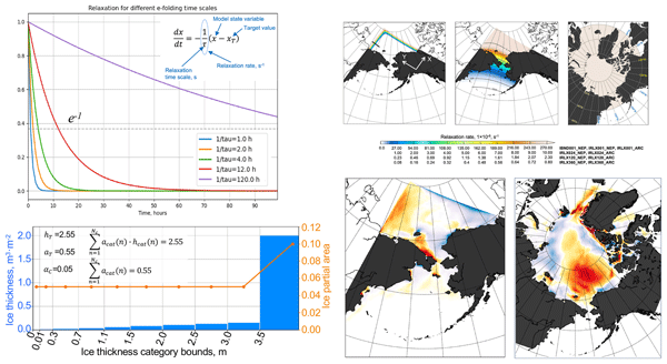
where x denotes the nudged variable, x_T is the target value, τ is the relaxation time scale, and t is time.

In SIS2, the relaxation is discretized using a backward Euler scheme, which is unconditionally stable (used here in the sense of absolute stability as defined in Quarteroni et al., 2000). The resulting equation is

$$\begin{array}{}\text{(6)}& x^{k+\mathrm{1}}={\left(\mathrm{1}+{\displaystyle \frac{\mathrm{\Delta }t}{\mathit{\tau }}}\right)}^{-\mathrm{1}}\left(x^k+{\displaystyle \frac{\mathrm{\Delta }t}{\mathit{\tau }}}{x}_{\mathrm{T}}\right).\end{array}$$

where k is the time index and Δt is the model time step.

4.2 Implementation of sea ice relaxation in SIS2

4.2.1 Conversion of the target variables

The relaxation algorithm consists of two main parts: initialization and application. The initialization routines are executed during the model setup phase, prior to the start of time integration. These routines identify ocean grid points where nudging will be applied, based on the specified relaxation rates, where the rate is greater than zero. The set of grid points selected based on the relaxation mask (defined as an input field and described in Sect. 4.3) is fixed prior to the start of the simulation and remains unchanged during time integration.

In the application step, the input ice concentration and thickness from external fields are first converted into the model-defined state variables before relaxation is applied. The target fields represent cell-mean ice concentration and thickness, whereas SIS2 defines variables per ice category. Therefore, the target ice variables must be distributed across the model's ice thickness categories in a way that conserves total ice mass.

The relationship between the target ice concentration (a_T) and the model ice concentration for thickness category n (a_cat(n)) is as follows

$$\begin{array}{}\text{(7)}& a_{\mathrm{T}}\equiv a_{\mathrm{tot}}=\sum _{n=\mathrm{1}}^{N_{\mathrm{c}}}{a}_{\mathrm{cat}}\left(n\right),\end{array}$$

where a_tot is the aggregated (grid-cell mean) ice concentration and N_c is the total number of ice thickness categories.

Similarly, the relationship between the target ice thickness (h_T) and the model thickness-category field is

$$\begin{array}{}\text{(8)}& h_{\mathrm{T}}\equiv v_{\mathrm{tot}}=\sum _{n=\mathrm{1}}^{N_{\mathrm{c}}}{a}_{\mathrm{cat}}\left(n\right)\cdot h_{\mathrm{cat}}\left(n\right),\end{array}$$

where v_tot is the total ice volume per unit grid-cell area (m³ m⁻²), equivalent to the cell-mean ice thickness provided in the target fields, and h_cat(n) denotes the mean ice thickness over the ice-covered area of category n. Once the target thickness is distributed across the categories, it is converted to the SIS2 units of mass per unit ice area (kg m⁻²) for each category n as

$$\begin{array}{}\text{(9)}& M_{\mathrm{cat}}\left(n\right)={\mathit{\rho }}_{\mathrm{ice}}{h}_{\mathrm{cat}}\left(n\right),\end{array}$$

where ρ_ice is sea ice density (Table 2).

4.2.2 Distribution of ice input variables by thickness categories

To ensure physical consistency of the prescribed target state, the target ice concentration and thickness are first remapped onto the SIS2 thickness categories in a manner that conserves total ice area and volume (Eqs. 7, 8). Because only bulk ice concentration and volume are prescribed, the problem is inherently underdetermined, and many different category distributions can satisfy the same constraints. Consequently, multiple redistribution strategies can be used to remap the target ice state onto the SIS2 thickness categories.

A simplest approach is to assign the entire target ice state to a single thickness category (the primary thickness category, n₀, defined below). This initialization conserves the prescribed bulk ice concentration and volume but leaves the remaining categories empty. Although formally valid, such a configuration represents a highly singular ice thickness distribution (ITD) and may require substantial redistribution during the first few model time steps as the model re-establishes a physically realistic multi-category structure. In particular, numerical formulations that depend on category ice area fractions can become sensitive when one or more categories contain little or no ice. In our experiments, single-category initializations were generally successful, but a small number of simulations failed during the early redistribution stage. The exact cause of these failures was not investigated in detail.

To provide a smoother initial ITD and avoid empty thickness categories, ice area and volume are redistributed across thickness categories up to the primary category (i.e., only categories thinner than n₀), while strictly conserving the prescribed bulk ice properties. This initialization strategy was used in all experiments presented here and exhibited stable behavior in our tests. Specifically, at each grid cell where the relaxation time scale is nonzero, the target ice state is distributed across the thickness categories (H_cat) using the procedure outlined below.

• i.

  Ice sufficiency constraint

  Redistribution is performed only when the target ice state is non-negligible, such that

  $$\begin{array}{}\text{(10)}& \left\{\begin{array}{l}{h}_{\mathrm{T}}\ge {\mathit{ϵ}}_{\mathrm{T}}\\ a_{\mathrm{T}}\ge {\mathit{ϵ}}_a\end{array}\right.,\end{array}$$

  where h_T and a_T denote the target ice thickness and concentration defined in Eqs. (7) and (8), respectively. The thresholds ${\mathit{ϵ}}_{\mathrm{T}}=\mathrm{1}\times {\mathrm{10}}^{-\mathrm{10}}$ m³ m⁻² and ${\mathit{ϵ}}_a=\mathrm{1}\times {\mathrm{10}}^{-\mathrm{10}}$ exclude infinitesimal ice states.

• ii.

  Identification of the primary thickness category

  The thickness category n₀ corresponding to the target ice thickness is identified as

  $$\begin{array}{}\text{(11)}& h_{\min }\left(n_{\mathrm{0}}\right)\le {\displaystyle \frac{h_{\mathrm{T}}}{a_{\mathrm{T}}}}<h_{max}\left(n_{\mathrm{0}}\right),\end{array}$$

  where h_min(n)=H_cat(n) and $h_{\max }\left(n\right)=H_{\mathrm{cat}}(n+\mathrm{1})$, i.e. the lower and upper bounds of the nth ice thickness category.

• iii.

  Initial assignment to the primary category

  The entire target ice thickness and concentration are initially assigned to category n₀ by

  $$\begin{array}{}\text{(12)}& {\displaystyle }{h}_{\mathrm{cat}}\left(n_{\mathrm{0}}\right)={\displaystyle \frac{h_{\mathrm{T}}}{a_{\mathrm{T}}}},\text{(13)}& {\displaystyle }{a}_{\mathrm{cat}}\left(n_{\mathrm{0}}\right)=a_{\mathrm{T}}.\end{array}$$

  The ice volume in category n₀ is $v_{\mathrm{cat}}\left(n_{\mathrm{0}}\right)=h_{\mathrm{cat}}\left(n_{\mathrm{0}}\right)\cdot a_{\mathrm{cat}}\left(n_{\mathrm{0}}\right)$.

• iv.

  Redistribution to thinner categories

  To populate thinner ice categories while maintaining conservation of the bulk ice properties defined by Eqs. (7) and (8), a portion of ice volume (Δv_cat) is sequentially redistributed from category n₀ to categories $n=\mathrm{1},\mathrm{\dots },n_{\mathrm{0}}-\mathrm{1}$, starting from the thinnest category. A minimum ice concentration threshold α_min is introduced to prevent artificial population of excessively thin or vanishing categories and is defined as

  $$\begin{array}{}\text{(14)}& {\mathit{\alpha }}_{min}=min\left\{{\mathit{\alpha }}_{\mathrm{C}},{\displaystyle \frac{a_{\mathrm{T}}}{n_{\mathrm{0}}}}\right\}.\end{array}$$

  Here, α_C is a tunable parameter controlling the amount of ice redistributed into thinner categories. In the experiments presented here, α_C=0.01. Smaller values of α_C restrict redistribution into thinner categories, retaining a larger fraction of ice volume in the primary category n₀. However, α_C should not be chosen too small, as this may produce categories with very small ice area fractions, partially reintroducing the numerical sensitivities associated with empty or nearly empty thickness categories discussed above.

  For each category n, a fixed ice volume

  $$\begin{array}{}\text{(15)}& \mathrm{\Delta }{v}_{\mathrm{cat}}={\mathit{\alpha }}_{min}\stackrel{\mathrm{̃}}{h},\end{array}$$

  is transferred from category n₀. Here, $\stackrel{\mathrm{̃}}{h}$ is defined as

  $$\begin{array}{}\text{(16)}& \stackrel{\mathrm{̃}}{h}=H_{\mathrm{cat}}\left(k\right)+{\mathit{ϵ}}_{\mathrm{0}},\end{array}$$

  where ${\mathit{ϵ}}_{\mathrm{0}}=\mathrm{1}\times {\mathrm{10}}^{-\mathrm{10}}$ m is an offset ensuring that the redistributed ice thickness remains within category bounds.

  The ice state in category n is updated as $h_{\mathrm{cat}}\left(n\right)=\stackrel{\mathrm{̃}}{h}$, and $a_{\mathrm{cat}}\left(n\right)={\mathit{\alpha }}_{min}$.

  The ice state in category n₀ is adjusted to conserve volume and concentration as

  $$\begin{array}{}\text{(17)}& {\displaystyle }{a}_{\mathrm{cat}}\left(n_{\mathrm{0}}\right)=max\mathit{\{}{a}_{\mathrm{cat}}\left(n_{\mathrm{0}}\right)-a_{\mathrm{cat}}\left(n\right),{\mathit{\alpha }}_{min}\mathit{\}},\text{(18)}& {\displaystyle }{v}_{\mathrm{cat}}\left(n_{\mathrm{0}}\right)=v_{\mathrm{cat}}\left(n_{\mathrm{0}}\right)-\mathrm{\Delta }{v}_{\mathrm{cat}},\text{(19)}& {\displaystyle }{h}_{\mathrm{cat}}\left(n_{\mathrm{0}}\right)={\displaystyle \frac{v_{\mathrm{cat}}\left(n_{\mathrm{0}}\right)}{a_{\mathrm{cat}}\left(n_{\mathrm{0}}\right)}}.\end{array}$$

  Redistribution proceeds sequentially until either all thinner categories up to (n₀−1) have been populated or the remaining ice concentration in category n₀ reaches the minimum threshold α_min, at which point redistribution is terminated.

• v.

  Conservation verification

  Following redistribution, the thickness-category fields are verified to conserve the prescribed target ice concentration and volume (Eqs. 7, 8).

  It should be noted that the redistribution procedure is not intended to reconstruct the true subgrid-scale ice thickness distribution from the prescribed bulk ice concentration and volume. The purpose of the redistribution algorithm is to generate a physically consistent multi-category SIS2 state that conserves the prescribed bulk ice properties while maintaining numerical stability during subsequent model integration. Alternative redistribution strategies, including methods designed to produce smoother category distributions, are possible.

To assess the robustness of the redistribution algorithm, it was tested using 5000 randomly generated target thickness–concentration pairs and exhibited stable behaviour across the tested range. Figure 2 illustrates the redistribution of ice across thickness categories for three representative cases. In Fig. 2a and b, the target ice thickness (2.55 m³ m⁻²) and concentration (0.95) are identical. However, the larger value of the parameter α_C in Eq. (14) used in Fig. 2b results in a greater fraction of ice being assigned to thinner categories compared to Fig. 2a. Figure 2a and c differ only in the total ice concentration (0.95 and 0.55, respectively), while the target ice volume per unit grid-cell area is held fixed. In Fig. 2c, all 10 thickness categories are populated (non-zero), because the lower target concentration implies a greater mean ice thickness over the ice-covered fraction of the cell, resulting in larger categorical ice thicknesses h_cat(n) (Eq. 8) and a larger value of n₀ according to Eq. (11). In all cases, the conservation constraints for total ice volume and ice concentration Eqs. (8) and (7) are satisfied.

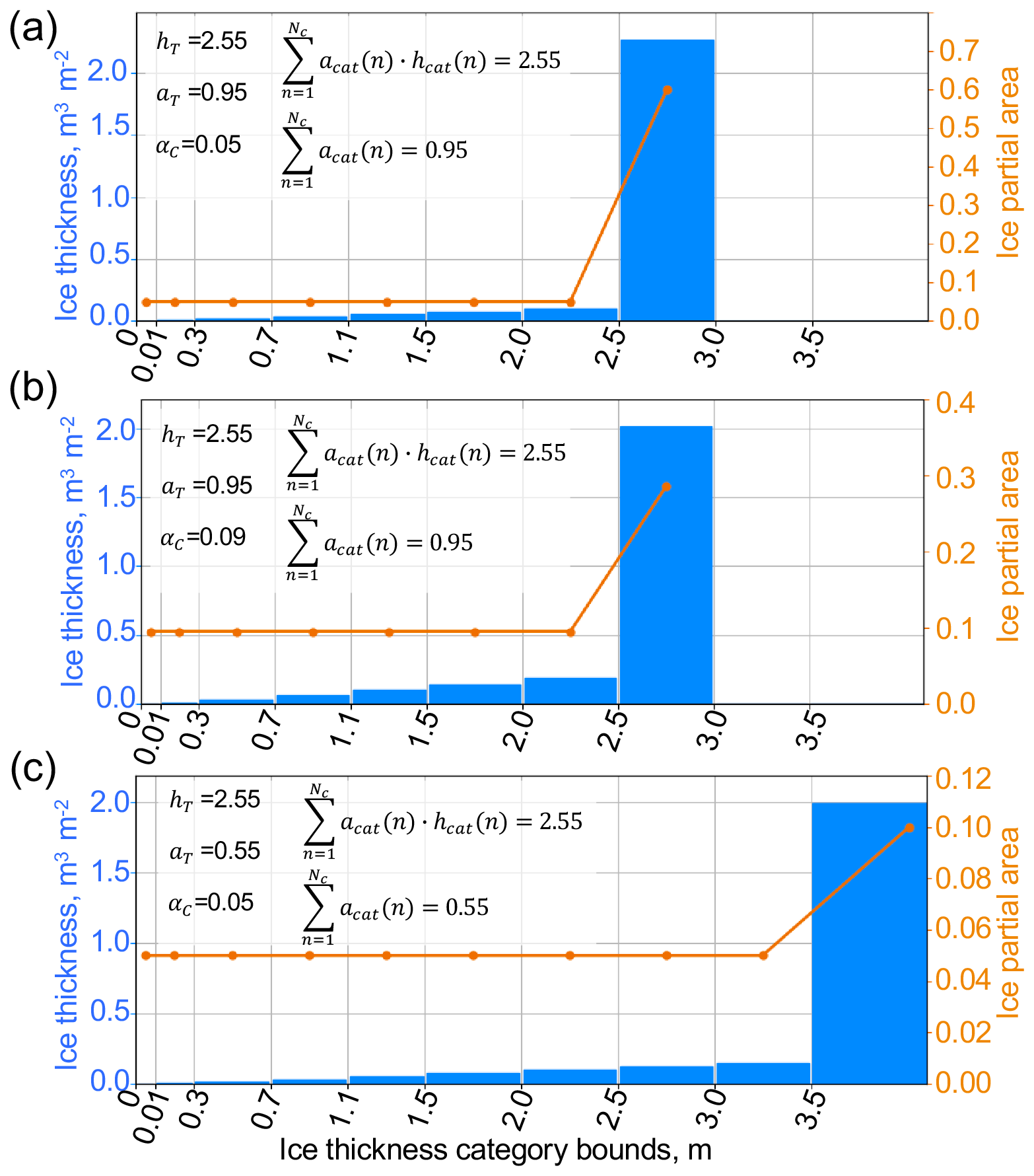
Figure 2 Example of the ice distribution algorithm showing ice thickness and partial ice area distribution for a fixed target ice thickness (2.55 m³ m⁻²) and ice concentration (0.95) with different values of the parameter α_C (0.05 in (a) and 0.09 in (b)), and for a fixed target ice thickness and α_C but different ice concentrations (0.95 in (a) and 0.55 in (c)). In all cases, the aggregated ice volume (Eq. 8) and ice concentration (Eq. 7) are conserved. The blue bars show the ice thickness distribution across the thickness categories (left y-axis). The orange dotted line shows the partial ice area in each category (right y-axis).

4.2.3 Update of sea ice temperature and salinity

During relaxation, ice volume is artificially modified as it is adjusted toward the target ice concentration and thickness. Each ice layer within each thickness category is characterized by salinity (S_i) and enthalpy (q_i). Because ice volume is altered during the relaxation procedure, salinity and enthalpy must be maintained within physically realistic bounds, particularly in grid cells transitioning from ice-free to ice-covered conditions. After the ice state has been relaxed to the target concentration and thickness, salinity and enthalpy are adjusted as follows.

For each ice layer in every thickness category, salinity is checked to ensure S_i≥S_bulk, where S_bulk is the prescribed bulk sea ice salinity (3.0 psu in this study). If this condition is not satisfied, salinity in all layers within that ice column is reset to S_bulk. Next, the ice enthalpy of each layer is evaluated to ensure that q_i≤q_max, where $q_{\max }=q\left(\stackrel{\mathrm{̃}}{T}\right)$ is the enthalpy of sea ice with salinity S_i at a temperature $\stackrel{\mathrm{̃}}{T}$ defined as

$$\begin{array}{}\text{(20)}& \stackrel{\mathrm{̃}}{T}=\min \mathit{\{}{T}_{\mathrm{frz}}\left(S_{\mathrm{i}}\right)-\mathrm{0.1},T_{\mathrm{ocn}}\mathit{\}},\end{array}$$

where T_frz(S_i) is the freezing point of sea ice of salinity S_i, and T_ocn is ocean surface temperature beneath the ice. The freezing point is offset by 0.1 °C to prevent rapid melting of newly formed ice immediately following the relaxation step. The use of the minimum operator ensures that newly initialized ice is not warmer than the underlying ocean surface temperature, preventing the ice enthalpy from being too high. If the condition is violated, the layer enthalpy is reset to q_max. For grid cells transitioning from ice-free to ice-covered conditions, S_i is initialized to S_bulk and q_i to q_max.

4.3 Spatial relaxation masks and rates

Spatially varying relaxation masks were designed to target lateral boundary regions or the interior ice state, depending on the domain configuration and forecasting objectives (Fig. 3). For the NEP10k configuration, two relaxation mask designs were implemented. In the first configuration, relaxation is applied only near the lateral boundaries in the Arctic portion of the domain (Fig. 3a). The maximum relaxation strength is imposed within the first five grid cells adjacent to the boundary and decays rapidly with distance from the boundary (Fig. 3b).

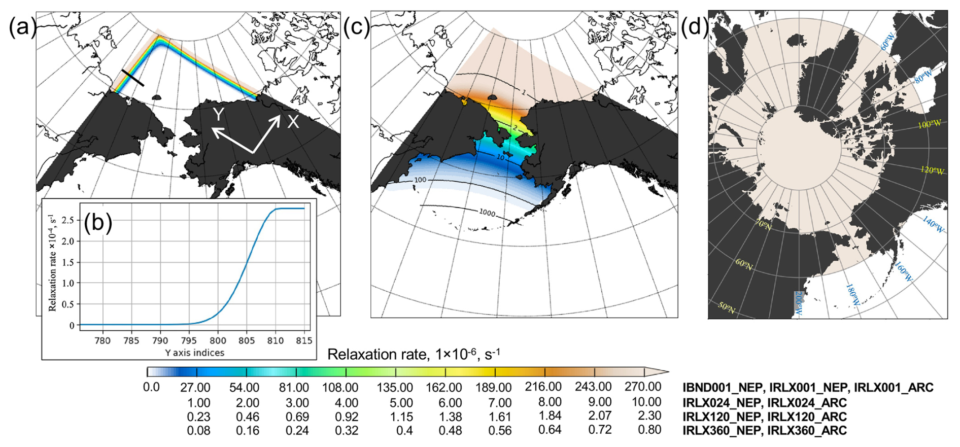
Figure 3 Spatial distribution of the relaxation time rates (s⁻¹) applied in the test experiments. Color shading indicates the relaxation rate (s⁻¹). (a) Relaxation applied along the lateral boundaries in the Arctic Ocean portion of the NEP10k domain. The black line marks the section along which the relaxation profile is shown in (b). The orientation of the model y and x axes is indicated in white. (b) Profile of the relaxation rate along the model y axis near the northwest boundary on the shelf (black line in (a)), demonstrating the rapid decay of the relaxation rate away from the boundary. (c) Relaxation applied over the entire polar portion of the NEP10k domain. Black contours indicate the multiplication factor of the minimum relaxation time scale (τ), where τ is the relaxation time scale defined in Eq. (5). The color bar shows the relaxation rate ($\frac{\mathrm{1}}{\mathit{\tau }}\times {\mathrm{10}}^{-\mathrm{6}}$ s⁻¹) with each row corresponding to a different strongest relaxation time scale (1, 24, 120, and 360 h). The corresponding experiment names are indicated. (d) Relaxation mask used in the ARC10K experiments, providing a spatially uniform relaxation rate (s⁻¹) over the Arctic Ocean north of 60° N.

In a second set of NEP10k experiments, relaxation is applied over the entire polar portion of the domain. The maximum relaxation strength spans the Arctic Ocean and decreases exponentially toward the southern Bering Sea. This design intentionally applies weaker constraints in the Bering Sea, where the model exhibits higher skill, while imposing stronger constraints in the Arctic Ocean to limit the influence of LBC errors on the interior ice state. The overall relaxation strength in these experiments is controlled by prescribing the strongest relaxation within the Arctic Ocean portion of the NEP10k domain.

In the ARC10k experiments, the influence of lateral boundary conditions on sea ice is minimal, because the model domain extends well beyond the typical extent of the marginal ice zone. Consequently, relaxation is used primarily to constrain the interior ice state. The relaxation mask in these experiments applies a spatially uniform relaxation rate north of 60° N (Fig. 3d).

The relaxation masks shown in Fig. 3 were designed for the specific objectives and domain configurations considered in this study. Although they provide suitable configurations for the NEP10k and ARC10k applications examined here, the optimal relaxation mask and rate may vary depending on the model domain, forecasting objectives, and dominant sources of model error.

5 Numerical simulations

The relaxation algorithm was evaluated using long-term and short-term numerical simulations to assess its robustness, its impact on model drift, and the sensitivity of simulated sea ice and ocean fields to relaxation parameters and time scales. The long-term simulations consist of existing multi-decadal NEP10k runs that were not specifically designed to test the relaxation algorithm but were originally produced to generate initial conditions for subsequent forecast applications. These simulations provide an opportunity to assess model drift and the cumulative impact of sea ice relaxation on the coupled ocean–ice system over extended time scales.

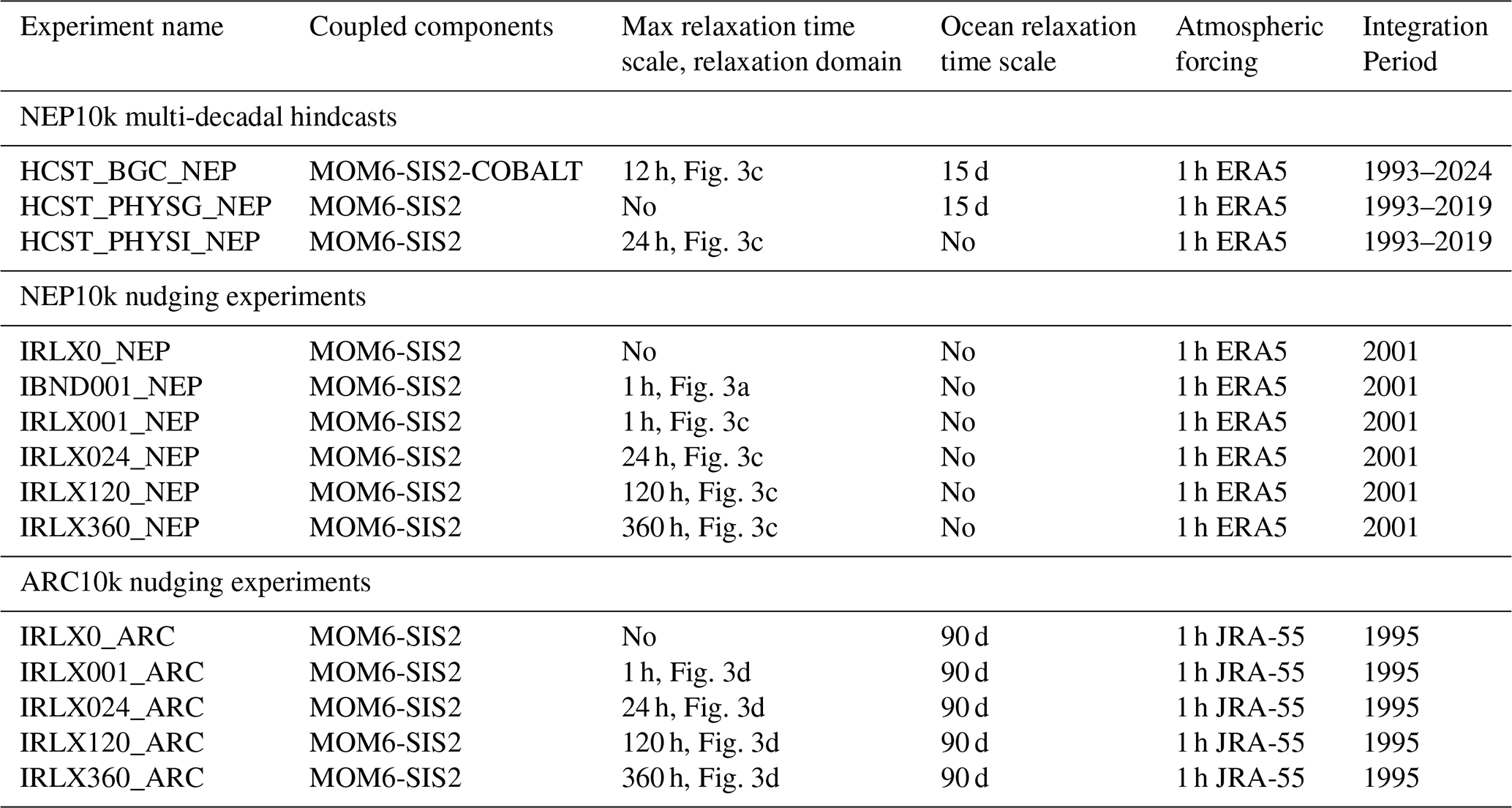
Short-term experiments were designed for this study and consist of one-year test runs aimed at evaluating the sensitivity of sea ice and ocean fields to relaxation and identifying any spurious effects introduced by the nudging on seasonal time scales. These experiments were conducted for both the NEP10k and ARC10k configurations using the spatial relaxation masks described in Sect. 4.3 (Fig. 3). Atmospheric forcing and target sea ice fields were derived from the reanalysis products used in the corresponding hindcast and forecast systems (ERA5 and JRA-55 for atmospheric forcing and PIOMAS for sea ice). A summary of all experiments is provided in Table 3.

Table 3 Numerical experiments with MOM6-SIS2 model.

5.1 Multi-decadal NEP10k simulations

The relaxation algorithm described here is a direct nudging technique, which does not explicitly add or remove salt and heat from the ocean, thus it is not mass- or energy conservative. England et al. (2022) showed that direct nudging implicitly adds or removes latent heat from the ocean when ice is removed or added during relaxation. Similarly, salt is implicitly added or removed from the ocean through the nudging process. In addition, direct nudging can trigger spurious ice melting due to noise introduced in the sea ice state during relaxation, especially under strong relaxation or where the underlying ocean is warmer than the freezing point. This spurious melting may lead to unphysical freshening of the surface ocean within the relaxation zone, causing drift in ocean surface salinity and temperature. To explore drifts in the ocean fields caused by ice nudging, we compare sea surface salinity (SSS) and sea surface temperature (SST) averaged over the Chukchi Sea region in the NEP10k domain (“Arctic Ocean” in Fig. 1c) across three multi-decadal hindcast simulations. Multi-decadal drift analysis is presented in Sect. 8.1.

5.1.1 NEP10k hindcast with biogeochemistry (HCST_BGC_NEP)

A multi-decadal NEP10k hindcast spanning the period 1993–2024 was analyzed (experiment HCST_BGC_NEP; Table 3). This simulation employed a fully coupled MOM6-SIS2 system with biogeochemistry (COBALT). The model configuration, forcing fields, and general hindcast setup follow Drenkard et al. (2025) (Tables 1 and 2) with the following differences: (i) SIS2 was configured with explicit ice ridging (mechanical redistribution); (ii) ocean temperature and salinity fields in the interior domain were nudged toward GLORYS12v1 ocean reanalysis (Lellouche et al., 2021) with a 15 d relaxation time scale; and (iii) the sea ice relaxation algorithm described in Sect. 4 was applied to nudge ice concentration and thickness. Sea ice was relaxed toward monthly PIOMASv2.1 fields using the relaxation mask shown in Fig. 3c, with a minimum (i.e., strongest) relaxation time scale of 12 h. The hindcast was initialized from a three-year spinup simulation.

5.1.2 NEP10k hindcast without ocean nudging (HCST_PHYSI_NEP)

To isolate the effects of sea ice nudging and eliminate corrections to ocean fields imposed by nudging toward GLORYS reanalysis, a second NEP10k multi-decadal hindcast with disabled ocean nudging was analyzed. This simulation employed the coupled MOM6-SIS2 system without biogeochemistry and covered the period 1993–2019. Sea ice relaxation was applied using the same relaxation mask shown in Fig. 3c. All other parameters and model settings were identical to those used in HCST_BGC_NEP.

5.1.3 NEP10k hindcast without ice relaxation (HCST_PHYSG_NEP)

A third hindcast employed the coupled MOM6-SIS2 system (physics only), with ocean temperature and salinity nudged toward GLORYS but without applying sea ice relaxation. The simulation covered the period 1993–2019. All parameters and settings were consistent with those in HCST_BGC_NEP.

5.2 Short-term test simulations

5.2.1 Experiments with the NEP10k

The NEP10k short-term test experiments analyzed in this study were initialized from the HCST_BGC_NEP hindcast simulation. All experiments were started on 1 January 2001, and integrated forward for one year as free-running simulations, forced by hourly ERA5 atmospheric fields. Ocean LBCs were prescribed from daily GLORYS12 ocean reanalysis fields.

A control experiment (IRLX0_NEP) was conducted without sea ice relaxation. In experiment IBND001_NEP, sea ice concentration and thickness were relaxed toward PIOMASv2.1 at the lateral boundaries using a 1 h relaxation time scale (Fig. 3a). In the remaining experiments, sea ice concentration and thickness were relaxed toward PIOMASv2.1 monthly fields using the same spatially varying relaxation mask applied over the polar portion of the domain (Fig. 3c), with increasing minimum (strongest) relaxation time scales: 1 h (IRLX001_NEP), 24 h (IRLX024_NEP), 120 h (IRLX120_NEP), and 360 h (IRLX360_NEP). These experiments are used to assess the impact of lateral boundary versus interior ice relaxation on sea ice state, edge position, and surface fields. Results are presented in Sect. 6.

5.2.2 Experiments with ARC10k

The ARC10k sensitivity experiments were initialized on 1 January 1995 from an existing hindcast simulation. As with the NEP10k experiments, the ARC10k simulations were integrated forward for one year. Atmospheric forcing was provided by hourly JRA-55 reanalysis fields, and ocean LBCs were prescribed from the GLORYS reanalysis. A control experiment (IRLX0_ARC) was conducted without sea ice relaxation. In the remaining experiments, sea ice state was nudged toward target fields derived from monthly PIOMASv2.1 data. The relaxation time scales used in these experiments were similar to those in the NEP10k simulations. However, unlike NEP10k, sea ice relaxation was applied uniformly across the entire Arctic north of 60° N (Fig. 3d). The experiments are analyzed in Sect. 7.

6 Results from NEP10k experiments

6.1 Control simulation (IRLX0_NEP)

6.1.1 Ice field differences

The impact of closed ice boundaries on the northern NEP10k domain is illustrated using the control simulation without ice relaxation (IRLX0_NEP; Table 3). Sea ice concentration and thickness differences are computed relative to three-month mean PIOMAS fields (Figs. 4a, 5a). During the first three months (JFM), the model develops positive sea ice concentration anomalies over the Bering Sea (Fig. 4b), while concentration anomalies in the Arctic Ocean remain small during winter, when sea ice coverage is near complete (Fig. 4a). In spring (AMJ) and summer (JAS), pronounced negative concentration anomalies emerge along the northeastern boundary north of Alaska. During the freeze-up season (OND), the model tends to overestimate ice concentration in the northern and northeastern Bering Sea and in the Chukchi Sea.

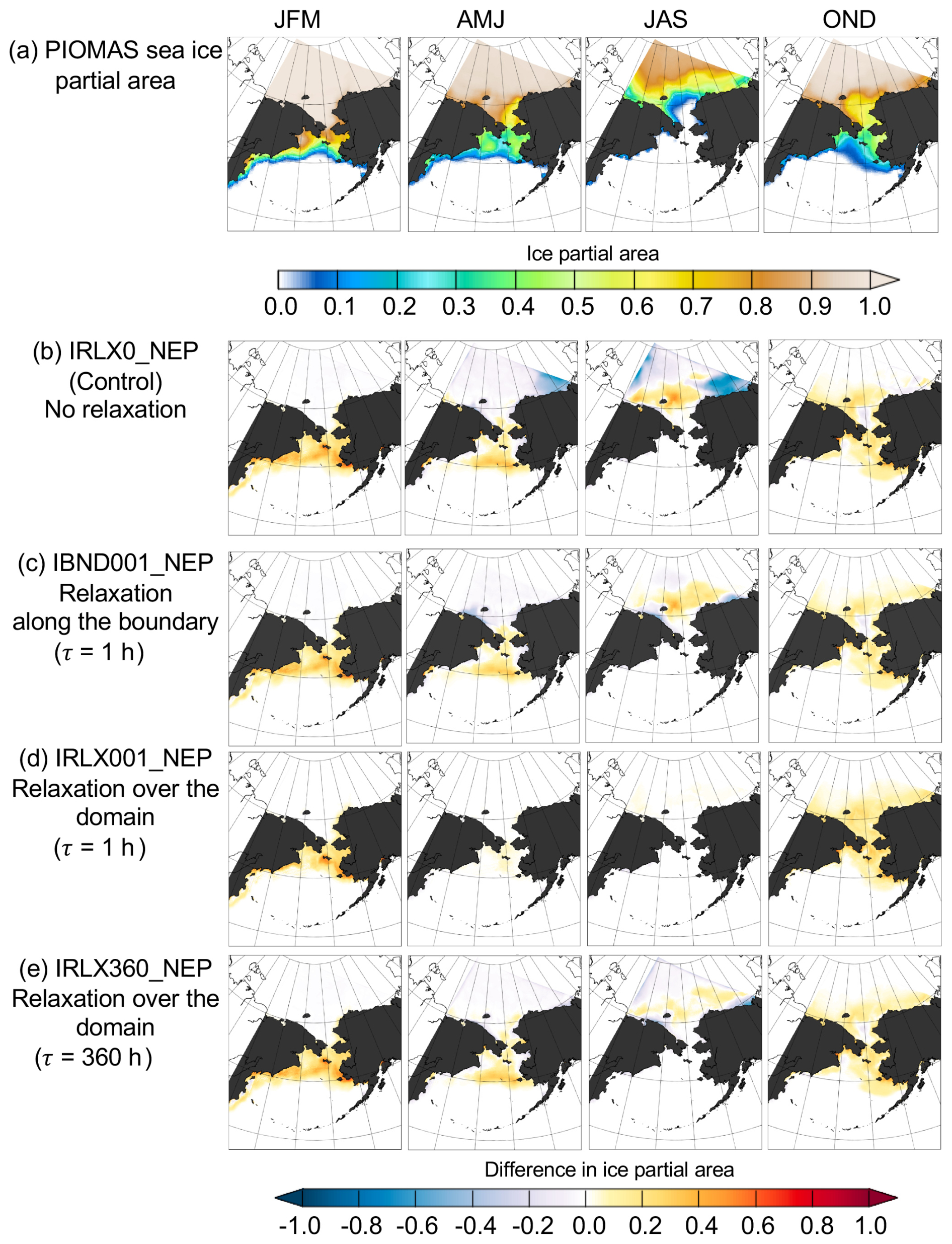
Figure 4 Maps of seasonal PIOMAS sea ice partial area (a) and differences in sea ice partial area between the NEP10k experiments and PIOMAS during 2001 (b–e). Columns correspond to seasons, with three-letter abbreviations indicating the averaging period (months). Each row in panels (b–e) represents a different experiment: (b) control simulation without relaxation (IRLX0_NEP); (c) relaxation applied along the lateral boundaries (IBND001_NEP); (d) relaxation applied over the polar portion of the NEP10k domain with a minimum relaxation time scale of 1 h (IRLX1_NEP); and (e) relaxation applied over the polar portion of the NEP10k domain with a minimum relaxation time scale of 360 h (IRLX360_NEP). Positive values indicate higher sea ice partial area in the model than in PIOMAS.

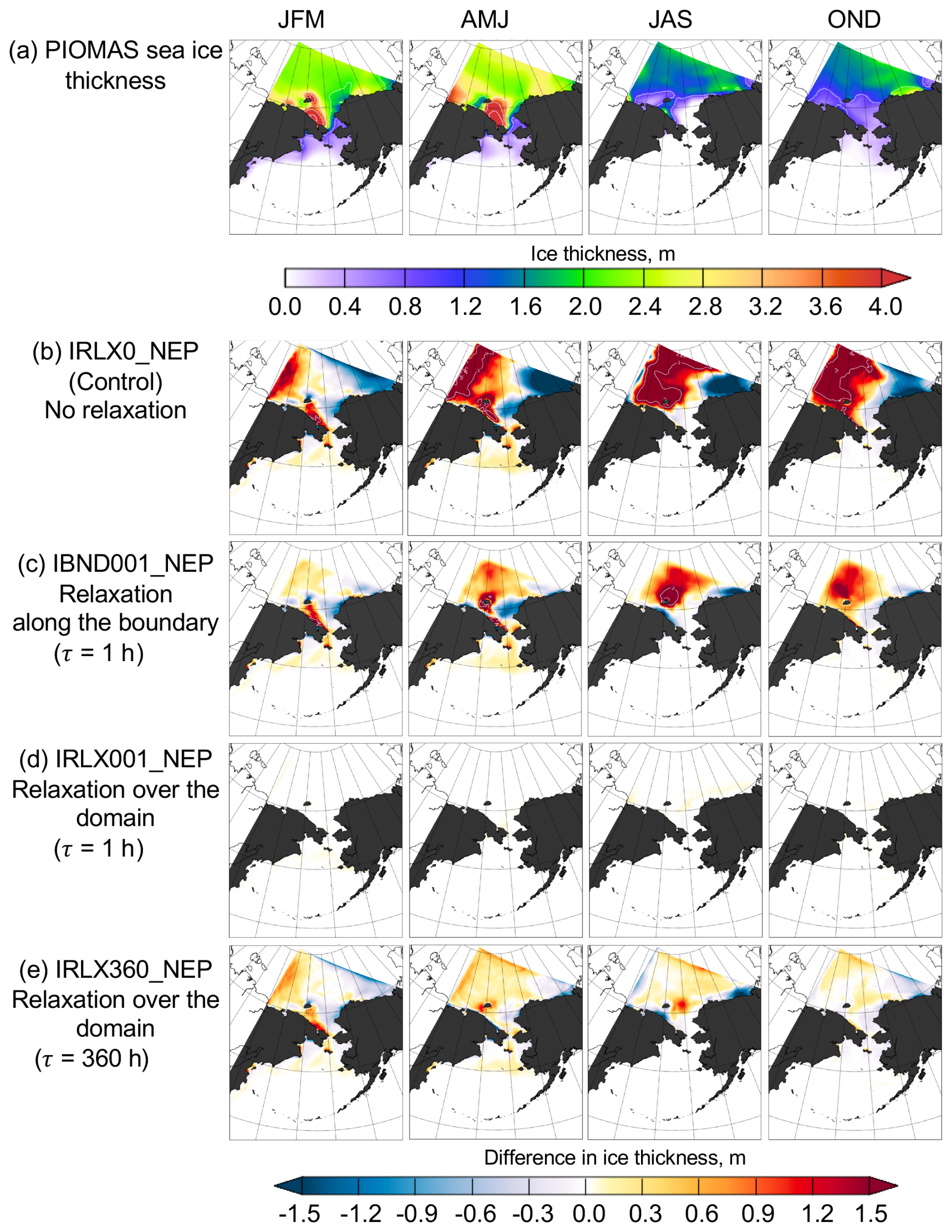
Figure 5 Maps of seasonal PIOMAS sea ice thickness (a) and differences in sea ice thickness between the NEP10k experiments and PIOMAS during 2001 (b–e). Columns correspond to seasons, with three-letter abbreviations indicating the averaging period (months). Each row in panels (b–e) represents a different experiment: (b) control simulation without relaxation (IRLX0_NEP); (c) relaxation applied along the lateral boundaries (IBND001_NEP); (d) relaxation applied over the polar portion of the NEP10k domain with a minimum relaxation time scale of 1 h (IRLX1_NEP); and (e) relaxation applied over the polar portion of the NEP10k domain with a minimum relaxation time scale of 360 h (IRLX360_NEP). Positive values indicate higher sea ice thickness in the model than in PIOMAS.

The effect of closed boundaries is more evident in sea ice thickness (Fig. 5b), with large positive anomalies rapidly emerging in the western Chukchi Sea. These arise from ice accumulation along the lateral boundary driven by prevailing anticyclonic Arctic winds, while the same circulation removes ice from the northeastern boundary. Ice continues to pile up throughout the integration, and by the end of the one-year simulation, thickness in the western Chukchi Sea exceeds the PIOMAS reference (Fig. 5a) by more than 2 m.

6.1.2 Sea ice performance metrics

These results are supported by a quantitative comparison of the control simulation with PIOMAS, performed separately for the Bering Sea and Arctic subdomains (Fig. 1c). In the Bering Sea, the control run exhibits large differences in ice concentration (blue line with bullets in Fig. 6a, c, e). The results closely overlap with those from IBND001_NEP, as explained in Sect. 6.2. The differences are particularly large during January–April, when sea ice extent and thickness peak. During this period, ice area and volume are overestimated (Fig. 6a, b), primarily due to positive biases in both ice concentration and thickness (Fig. 6d, e). In summer, when the Bering Sea is largely ice-free, differences in all sea ice metrics are substantially reduced (Fig. 6c–f).

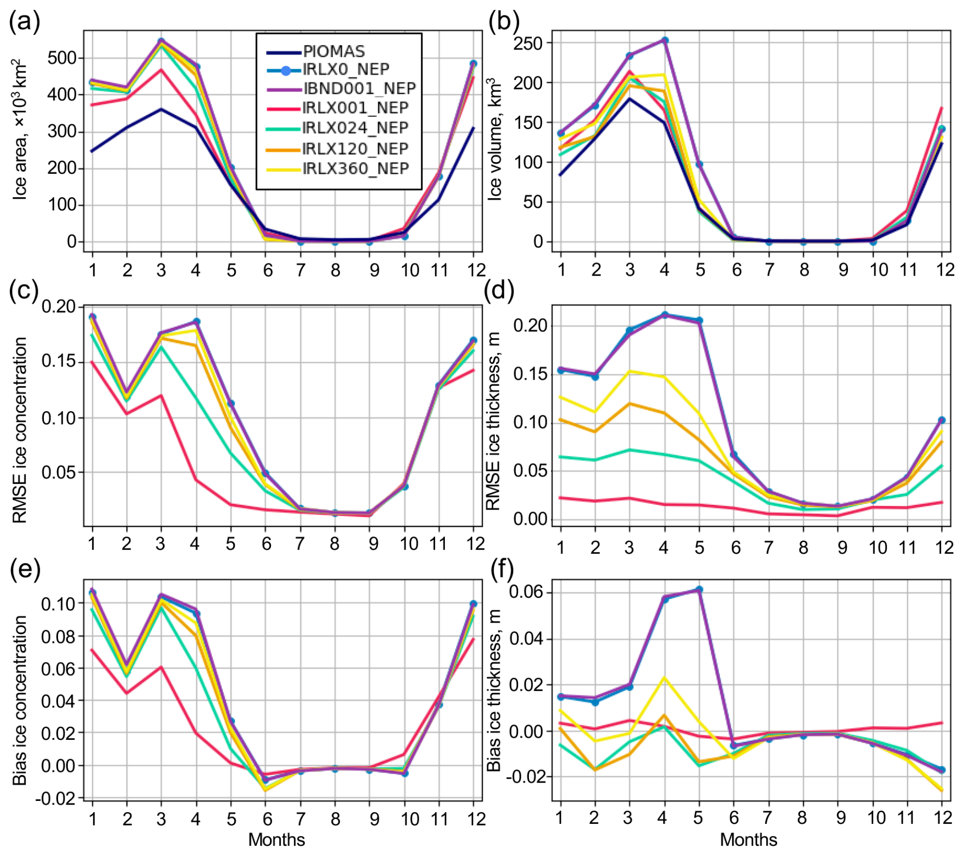
Figure 6 Statistics of sea ice characteristics in the Bering Sea from the NEP10k experiments designated with different colors shown in the legend. (a) Ice area (×10³ km²). (b) Ice volume (km³). PIOMAS estimates in (a) and (b) are shown by dark blue lines. (c) RMSE of ice concentration between the NEP10k simulations and PIOMAS. (d) RMSE of ice thickness between the NEP10k simulations and PIOMAS. (e) Bias of ice concentration in the NEP10k simulations relative to PIOMAS. (f) Bias of ice thickness (m) in the NEP10k simulations relative to PIOMAS. The horizontal axis denotes calendar month. Note that the control run (IRLX0_NEP; blue line with a bullet) overlaps with the IBND001_NEP (purple line), due to similar results as discussed in the text.

Figure 7 Statistics of sea ice characteristics in the Arctic portion of the domain from the NEP10k experiments. (a) Ice area (×10³ km²). (b) Ice volume (×10³ km³). PIOMAS estimates in (a) and (b) are shown with dark blue lines. (c) RMSE of ice concentration between the NEP10k simulations and PIOMAS. (d) RMSE of ice thickness between the NEP10k simulations and PIOMAS. (e) Bias of ice concentration in the NEP10k simulations relative to PIOMAS. (f) Bias of ice thickness (m) in the NEP10k simulations relative to PIOMAS. The horizontal axis denotes calendar month.

Differences are more pronounced in the Arctic portion of the NEP10k domain (Fig. 7), where the statistics exhibit a strong seasonal cycle. Differences in ice concentration are relatively small during winter and late fall, when the region is nearly fully ice-covered (Fig. 7a, c, e). In contrast, during summer the control simulation poorly reproduces the spatial distribution of ice concentration, with RMSE values exceeding 0.25 and a systematic underestimation of partial ice area, leading to an underprediction of total ice area (Fig. 7a, c, e). The simulation also shows substantial differences in ice thickness (Fig. 7d, f), resulting in a marked overestimation of ice volume beginning in April and increasing through the end of the integration (Fig. 7b).

6.1.3 Sea ice edge position

In the IRLX0_NEP control simulation, the simulated ice edge closely matches PIOMAS during periods when the ice edge lies within the Bering Sea (January–March and November–December; Fig. 8). From May through October, as the ice edge retreats into the Arctic Ocean, the simulation exhibits larger discrepancies. This part of the NEP10k domain is strongly influenced by the presence of closed boundaries, which contribute to substantial uncertainties in simulated ice characteristics and lead to increased errors in predicting the ice edge location.

Figure 8 MHD score (km) for the monthly ice edge contours derived from the NEP10k simulations relative to PIOMAS. The scores are computed using the 0.15 ice concentration contours. Lower scores indicate a closer match between the ice edge position in the simulation and PIOMAS. The horizontal axis denotes calendar month.

Overall, the NEP10k control experiment exhibits substantial errors in sea ice characteristics across the Arctic portion of the NEP10k domain and the northern Bering Sea, primarily due to the proximity of ice closed boundaries. The most prominent issues include unrealistic spatial distribution of ice and excessive ice thickness.

6.2 NEP10k with lateral boundary relaxation

6.2.1 Ice field differences

The IBND001_NEP experiment was designed to reduce the impact of LBCs on the interior ice state in the NEP10k domain. Compared to the control run, differences in ice concentration between IBND001_NEP and PIOMAS show improvement over the Arctic portion of the domain from January through September (Fig. 4c). In particular, relaxation along the boundaries reduces the strong negative anomaly near the northeastern boundary in the Beaufort Sea present in IRLX0_NEP during summer (Fig. 4b). No notable improvement is observed during October–December. Boundary relaxation has no discernible impact on ice concentration in the Bering Sea, where differences remain nearly identical to those in IRLX0_NEP. This supports the assumption that the Bering Sea ice state is weakly sensitive to Arctic LBCs.

Sea ice thickness in the Arctic Ocean is also affected by boundary relaxation, with reduced disagreement between IBND001_NEP and PIOMAS (Fig. 5c). Differences are zero within the relaxation region along the northwestern and northeastern boundaries. Outside the relaxation region, two unrealistic features present in IRLX0_NEP, ice pileup along the northwestern boundary and ice depletion along the northeastern boundary (Fig. 5b), are eliminated. However, Arctic interior ice remains too thick, with differences exceeding 2 m during July–September. Consistent with the ice concentration results, sea ice thickness in the Bering Sea is largely unchanged relative to IRLX0_NEP.

6.2.2 Sea ice performance metrics

In the Bering Sea, performance metrics for IBND001_NEP are nearly identical to those from the control run (Fig. 6), reflecting the low sensitivity of the regional ice state to Arctic LBCs. In contrast, IBND001_NEP shows substantial improvement across all Arctic ice metrics compared to IRLX0_NEP (Fig. 7).

6.2.3 Sea ice edge position

The sea ice edge position in IBND001_NEP is similar to IRLX0_NEP during winter and late fall (Fig. 8), when the ice edge lies in the Bering Sea and the influence of LBCs is minimal. During June–August, IBND001_NEP produces a more realistic ice edge, closer to the PIOMAS-derived contour, consistent with improved ice concentration in the Arctic Ocean. Overall, lateral boundary relaxation modestly improves the Arctic ice state in NEP10k. To further evaluate the approach, relaxation is next applied over the entire polar domain (Fig. 3c) to reduce misfits in ice concentration and thickness.

6.3 NEP10k with domain-wide relaxation

6.3.1 Ice field differences

Seasonal ice concentration differences between the NEP10k experiments and PIOMAS show clear improvement during April–September when relaxation is applied over the Arctic portion of the domain. Among the nudged experiments, IRLX001_NEP (strongest relaxation; Fig. 4d) exhibits the smallest concentration differences. In contrast, improvements relative to the control run (IRLX0_NEP; Fig. 4b) are less evident during the cold seasons (January–March and October–December). During January–March, concentration differences of approximately 0.1–0.4 persist in the Bering Sea, consistent with the weaker relaxation applied in that region. During October–December, the differences are smaller (approximately 0.1–0.2) but extend beyond the Bering Sea into the Chukchi and coastal Beaufort Seas, with magnitudes comparable to those in the non-nudged experiment. As the relaxation time scale increases, concentration differences become more pronounced during April–June and July–September, as illustrated by the weakest-relaxation experiment, IRLX360_NEP (Fig. 4e). By contrast, the sensitivity of ice concentration to the relaxation time scale is less apparent during January–March and October–December.

The impact of ice relaxation is more pronounced for ice thickness, as demonstrated by the IRLX001_NEP and IRLX360_NEP experiments (Fig. 5d, e). Throughout the integration period, all nudged experiments show substantial improvement relative to both the control run (Fig. 5b) and the lateral-boundary relaxation experiment (IBND001_NEP; Fig. 5c). In IRLX001_NEP, thickness differences are generally close to zero over most of the domain. The magnitude of the differences increases as the relaxation weakens, becoming noticeable in IRLX360_NEP (Fig. 5e), but remaining substantially smaller than in IRLX0_NEP and IBND001_NEP. Notably, even the weakest relaxation constrains ice thickness to within approximately 0.5 m of PIOMAS across most of the domain, whereas substantially larger differences persist in IBND001_NEP (Fig. 5c).

6.3.2 Sea ice performance metrics

Because the relaxation rate is weaker in the Bering Sea than in the Arctic (Fig. 3c), a reduced sensitivity to nudging is expected there. In the Bering Sea, all NEP10k experiments overestimate total ice area during months with ice cover (Fig. 6a), reflecting a persistent positive bias in ice concentration relative to PIOMAS (Fig. 6e). Compared to the control run, nudging improves ice area and volume estimates from January to May, with IRLX001_NEP (strongest relaxation) showing the best agreement with PIOMAS (Fig. 6a, b). During the freeze-up period (October–December), however, all experiments similarly overestimate ice area and volume, indicating limited sensitivity to the relaxation strength. The RMSE and bias statistics further demonstrate the benefits of nudging, particularly for ice thickness (Fig. 6c–f). Ice-thickness RMSE decreases monotonically with increasing relaxation strength, and even weak nudging (IRLX360_NEP) substantially reduces errors relative to both the control and lateral-boundary relaxation experiments. Ice-thickness biases remain small (< 0.03 m) in all nudged simulations, with the smallest biases occurring in IRLX001_NEP.

In the Arctic portion of the domain, where relaxation is applied uniformly over most of the region, the impact of nudging is evident across all metrics (Fig. 7). Nudged simulations closely reproduce PIOMAS ice area and volume from January through September, representing a marked improvement over the control (IRLX0_NEP) and IBND001_NEP, both of which diverge from PIOMAS after April (Fig. 7a, b). Ice concentration RMSE and bias are reduced in all nudging experiments, with IRLX001_NEP consistently exhibiting the highest skill (Fig. 7c, e), although errors increase during October as rapid ice formation begins. In contrast, ice thickness RMSE and bias remain low throughout the simulation in all nudged experiments (Fig. 7d, f), with error magnitudes again decreasing with increasing relaxation strength.

6.3.3 Sea ice edge position

The IRLX001_NEP experiment outperforms all other NEP10k simulations in predicting the ice edge location, exhibiting the lowest MHD score throughout the integration period (Fig. 8). The remaining experiments rank consistently with relaxation strength, with the control run generally exhibiting the poorest skill. The spread across the simulations is small from January to April and from November to December but increases during May to October. Again, the impact of nudging is less pronounced during winter and late fall, when the ice edge lies in the Bering Sea, where relaxation is substantially weaker than in the Arctic portion of the domain.

7 Results from ARC10k experiments

7.1 Control simulation (IRLX0_ARC)

7.1.1 Ice field differences

The ARC10k control simulation (IRLX0_ARC) has a closer match with the PIOMAS reanalysis (Fig. 9a) than the IRLX0_NEP experiment, because the lateral boundaries are located far from the ice edge. During winter and spring, the IRLX0_ARC ice concentration fields show good agreement with the PIOMAS reanalysis except for the Bering Sea (Fig. 9b). However, the model has difficulty reproducing the ice edge along the East Greenland Current and within the MIZ of the Barents Sea, where ARC10k overestimates ice concentration by more than 0.5. During summer (JAS), the model underestimates ice concentration on the Eurasian shelf by ∼ 0.1–0.3. During the freeze-up season (OND), differences increase over the shelf seas. Ice thickness differences remain significant in IRLX0_ARC throughout the year (Fig. 10b). The model consistently overestimates ice thickness, by more than 0.8 to 1 m relative to PIOMAS (Fig. 10a), in regions such as the East Greenland Current, the Beaufort Sea, and the Chukchi Sea.

Figure 9 Maps of seasonal PIOMAS sea ice partial area (a) and differences in sea ice partial area between the ARC10k experiments and PIOMAS during 1995 (b–d). Columns correspond to seasons, with three-letter abbreviations denoting the averaging period (in months). Each row in panels (b)–(d) represents a different experiment: (b) control simulation without relaxation (IRLX0_ARC); (c) relaxation applied north of 60° N with a relaxation time scale of 1 h (IRLX1_ARC); and (d) relaxation applied north of 60° N with a relaxation time scale of 360 h (IRLX360_ARC). Positive values indicate higher sea ice partial area in the model than in PIOMAS.

7.1.2 Sea ice performance metrics

The ARC10k control simulation consistently overestimates both sea ice area (Fig. 11a) and volume (Fig. 11b) relative to PIOMAS. The error in ice concentration remains high throughout the year, exceeding 0.13–0.15 (Fig. 11c), and is positive (Fig. 11e). The IRLX0_ARC experiment also exhibits substantial errors in ice thickness, with deviations reaching up to 0.5 m compared to PIOMAS (Fig. 11d). The mean thickness errors are predominantly positive, except in March and April, indicating that the model tends to overestimate ice production relative to the reference data (Fig. 11f).

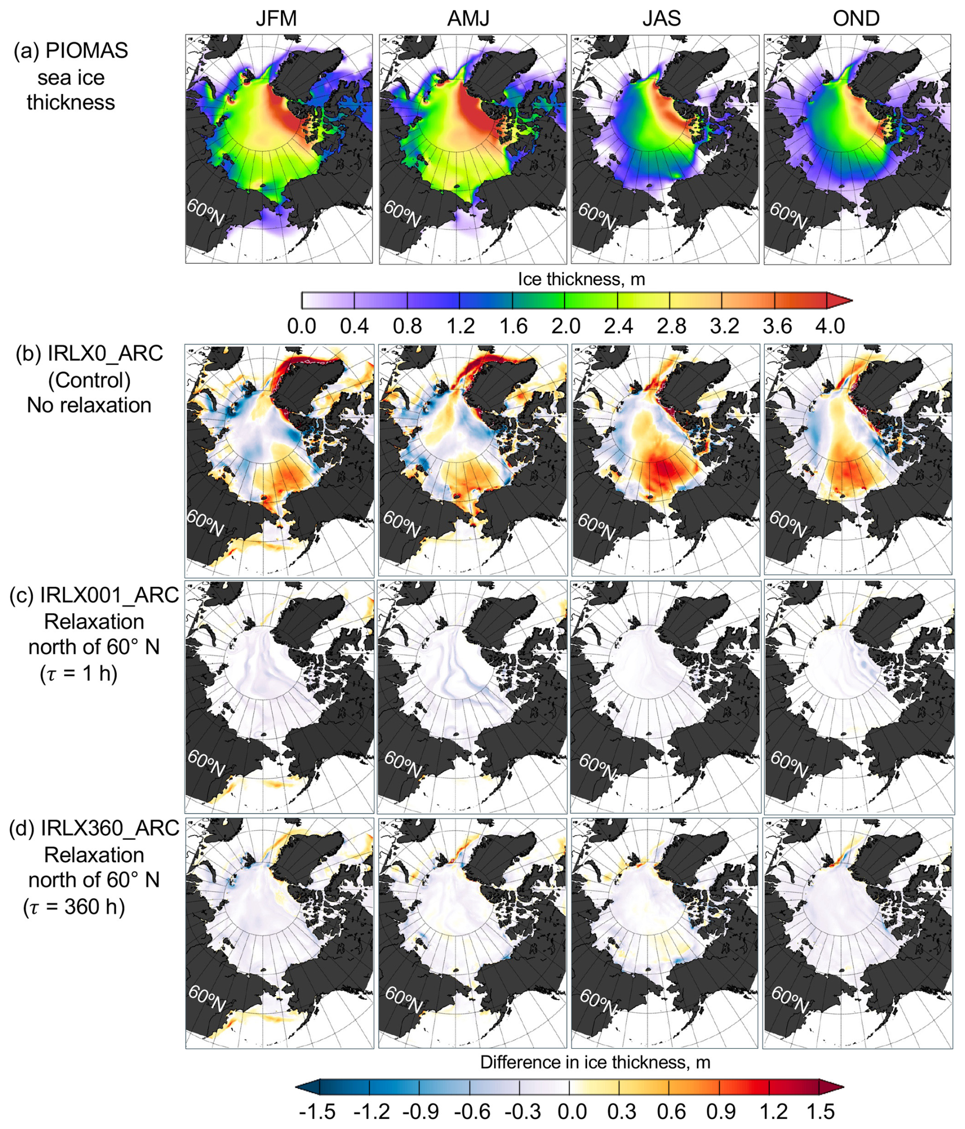
Figure 10 Maps of seasonal PIOMAS sea ice thickness (a) and differences in sea ice thickness (b–d) between the ARC10k experiments and PIOMAS during 1995. Columns correspond to seasons, with three-letter abbreviations denoting the averaging period (in months). Each row in panels (b)–(d) represents a different experiment: (b) control simulation without relaxation (IRLX0_ARC); (c) relaxation applied north of 60° N with a relaxation time scale of 1 h (IRLX1_ARC); and (d) relaxation applied north of 60° N with a relaxation time scale of 360 h (IRLX360_ARC). Positive values indicate higher sea ice thickness in the model than in PIOMAS.

Figure 11 Statistics of sea ice characteristics from the ARC10k experiments. (a) Ice area (×10³ km²). (b) Ice volume (km³). PIOMAS estimates in (a) and (b) are shown with dark blue lines. (c) RMSE of ice concentration between the ARC10k simulations and PIOMAS. (d) RMSE of ice thickness between the ARC10k simulations and PIOMAS. (e) Bias of ice concentration in the ARC10k simulations relative to PIOMAS. (f) Bias of ice thickness (m) in the ARC10k simulations relative to PIOMAS. The horizontal axis denotes calendar month.

7.1.3 Sea ice edge position

The position of the sea ice edge in the IRLX0_ARC experiment is relatively close to the PIOMAS derived estimate during the cold months (January through March and December) (Fig. 12). However, during the melt and freeze-up seasons, the accuracy of the simulated ice edge declines, consistent with the NEP10k control run.

Figure 12 MHD score (km) for the monthly ice edge contours derived from the ARC10k simulations and PIOMAS. The horizontal axis denotes calendar month.

7.2 ARC10k relaxation experiments

7.2.1 Ice field differences

Applying relaxation reduces the overestimation of ice concentration in the marginal ice zone (MIZ) observed in IRLX0_ARC (Fig. 9). Summer ice concentration is substantially improved in the relaxation experiments, with IRLX001_ARC exhibiting the smallest differences relative to PIOMAS (Fig. 9c). Even the weakly nudged experiment (IRLX360_ARC; Fig. 9d) shows improvement, although overestimation of ice concentration in the MIZ remains noticeable. Consistent with the NEP10k experiments, nudging produces only modest improvements over the shelf seas during OND. During this period, ice concentration differences over the shelf seas remain evident, although relatively small (approximately 0.1–0.2), and are comparable to those in the control run without relaxation. These persistent autumn differences may reflect a colder simulated ocean state, likely arising from differences between the JRA-55 atmospheric forcing used here and the NCEP/NCAR Reanalysis 1 forcing used in PIOMAS, which are not directly corrected by sea ice nudging.

As in the NEP10k experiments, the effect of nudging is more pronounced in the ice thickness fields (Fig. 10c, d). Regions south of the 60° N relaxation boundary show weaker improvements, partially retaining the discrepancies seen in the control run. Relaxation effectively constrains ice thickness toward PIOMAS, resulting in consistently small thickness differences throughout the year across all nudging experiments.

7.2.2 Sea ice performance metrics

The ARC10k relaxation experiments show improved ice area estimates relative to the control run (IRLX0_ARC) from January through July, with closer agreement to PIOMAS (Fig. 11a). During the freeze-up months (October–December), however, relaxation has little impact on ice area. From January to September, RMSE and bias in ice concentration (Fig. 11c, e) behave as expected, with stronger nudging generally yielding better performance. Consistent with the NEP10k simulations, the impact of relaxation during freeze-up is reduced, and all nudging experiments exhibit increased RMSE and bias in ice concentration during October–December.

Ice-thickness RMSE is substantially lower in all nudging experiments compared to the control run, indicating an overall improvement throughout the year (Fig. 11d). However, contrary to expectations, the strongest relaxation experiment (IRLX001_ARC) does not achieve the lowest RMSE. Instead, IRLX024_ARC, which applies slightly weaker relaxation, performs best. Ice-thickness bias is generally negative in the nudged simulations, whereas the control run exhibits a positive bias for most of the year, except in March and April when it becomes slightly negative and near zero (Fig. 11f). Overall, IRLX024_ARC shows the best ice-thickness performance in terms of both RMSE and bias, outperforming the strongest-relaxation configuration.

7.2.3 Sea ice edge position

Relaxation of ice concentration and thickness improves the accuracy of the simulated ice edge position, as indicated by notably lower MHD values in the nudging experiments compared to the control run, except for IRLX360_ARC in October (Fig. 12). Overall, model skill aligns with expectations: the experiment with the strongest nudging achieves the lowest MHD, and skill generally decreases as the strength of the nudging weakens.

8 Model drift and surface field biases

This section examines model drift in SSS and SST induced by sea ice relaxation, based on multi-decadal NEP10k hindcast simulations. Short-term impacts of relaxation on surface fields are assessed using the NEP10k relaxation experiments.

8.1 Multi-decadal NEP10k drift analysis

Time series of the SSS and SST averaged over the Arctic subregion (Fig. 1c) from the multi-decadal NEP10k hindcast simulations are shown in Fig. 13a and b. These series exhibit natural interannual variability, with no discernible long-term drift in either field, suggesting that while ice relaxation affects the surface ocean, it does not introduce spurious drift in SST or SSS.

Figure 13 Analysis of linear trends in SSS and SST time series averaged over the Arctic subregion within the NEP10k hindcast simulations (Table 3). (a) Time series of SSS. (b) Time series of SST. (c) March (winter) SSS with least-square linear fits by the hindcasts. (d) March SST with least-square linear fits by the hindcasts. (e) September (summer) SSS with least-square linear fits. (f) September SST with least-square linear fits. (g) Summary linear regression parameters for SSS and associated p-values (p₀) for testing the null hypothesis (H₀: α₁=0). (h) Same as (g) but for SST. Bold values indicate significant slopes at the 0.05 significance level.

The SST from the hindcast without ocean nudging toward GLORYS target fields but with ice relaxation (HCST_PHYSI_NEP) closely follows that from the hindcast with both ice and ocean nudging (HCST_BGC_NEP). In contrast, the hindcast without ice relaxation (HCST_PHYSG_NEP) disagrees with the other two during summer (Fig. 13b). Both ice relaxed simulations capture anomalously high SSTs in the Chukchi Sea during the summer of 2007, with spatially averaged SSTs exceeding 4 °C, whereas the simulation without ice relaxation (HCST_PHYSG_NEP) shows only modest warming, barely exceeding 1 °C. The ice-relaxed hindcasts align more closely with satellite observations, which recorded SSTs exceeding 7 °C in the Chukchi Sea that summer (Steele et al., 2008). These anomalous warm conditions were associated with reduced sea ice cover, and ice relaxation improves the timing of the seasonal sea ice retreat from this sea and the consequent lower spatially averaged albedos. The improved representation of sea ice in HCST_BGC_NEP and HCST_PHYSI_NEP enabled better reproduction of the observed SST anomalies.

To further assess potential long-term drift, trends in March (winter) and September (summer) surface fields were analyzed. All three simulations show a small, negative, but not statistically significant, trend in winter SSS (Fig. 13c, g), with HCST_PHYSI_NEP closely matching HCST_BGC_NEP. For summer SSS (Fig. 13e, g), the two ice-relaxed hindcasts exhibit similar positive (though again not significant) trends, while HCST_PHYSG_NEP shows a small negative trend, suggesting a different long-term evolution of summer salinity in the absence of ice nudging.

For winter SST (Fig. 13d), all three hindcasts are in strong agreement, showing a statistically significant positive trend (Fig. 13h). In summer SST, all simulations display positive trends, but the trend is statistically significant only in the ice-relaxed experiments.

8.2 Differences in SSS and SST from the short-term experiments

To assess potential unphysical impacts of ice relaxation on ocean fields within the relaxation zone, we analyze spatially averaged SST and SSS from the ice-relaxed experiments and the control run. Although the nudging experiments are too short to reveal long-term drift, significant errors introduced by relaxation, such as unphysical freshening or warming, could still appear in these time series.

In the Bering Sea, SST differences between the nudging experiments and the control run (Fig. 14a) are minimal, indicating negligible impact of relaxation. SSS differences (Fig. 14b) are more pronounced, exhibit seasonal variability, but generally diminish by the end of the year, suggesting no persistent annual drift.

Figure 14 Time series of the sea surface temperature (SST) and salinity (SSS) fields from the NEP10k and ARC10k simulations. (a) SST from the NEP10k control run (IRLX0_NEP) and nudging experiments averaged over the Bering Sea region (Fig. 1c). (b) Same as (a) but for SSS. (c) SST from the NEP10k control run (IRLX0_NEP) and nudging experiments averaged over the Arctic Ocean region of the domain. (d) Same as (c) but for SSS. (e) SST from the ARC10k control run (IRLX0_ARC) and nudging experiments averaged over the region poleward of the 60° N (relaxation region). (f) Same as (e) but for SSS.

In the Arctic subregion, summer SSTs in the control run are substantially warmer than in the nudging experiments (Fig. 14c), primarily due to large negative ice concentration anomalies from May through September (Fig. 7c, e), which increase open-water area and heat absorption. The SSS time series, however, do not converge by the end of the year (Fig. 14d). The nudging experiments show lower SSS values than the control run, which is attributed to reduced ice production in the presence of ice relaxation, as indicated by lower ice volume in the Arctic portion of the NEP10k domain (Fig. 7b). A simple estimate, neglecting vertical mixing and horizontal advection and also assuming a regional area of 1.74 × 10⁶ km² and a sea ice salinity of 3.4, shows that December ice volume difference between the control run and the nudging experiments (∼ 1626 km³) could raise the upper 10 m ocean salinity from 29.5 to 30, consistent with the observed SSS differences (Fig. 14d).

In the ARC10k, SST differences are small, with the control run slightly colder than the ice-relaxed experiments during May to July (Fig. 14e), consistent with a larger sea ice area in the control during this period (Fig. 11a). SSS differences are minimal during the cold months but become more noticeable during the melt season and freeze-up (Fig. 14f), disappearing by the end of the year, indicating no annual drift.

9 Discussion

The primary objective of these experiments was to evaluate the sea ice relaxation method implemented in SIS2 and its impact on ice and ocean surface properties. The method was tested using two regional configurations, NEP10k and ARC10k, by comparing simulations with and without ice relaxation to assess (i) how closely the relaxed ice concentration and thickness match the prescribed target fields, and (ii) whether the nudging preserves physically plausible sea ice and ocean conditions without introducing drift in SST or SSS.

Relaxation applied only along the lateral boundaries of the NEP10k domain produces modest improvements in the Arctic ice state. This limited impact reflects the fact that boundary relaxation constrains ice concentration and thickness but does not directly correct ice dynamics, primarily serving to mitigate the effects of the no-flow boundary condition. A more effective constraint would require adjusting ice velocities both parallel and normal to the boundaries. Importantly, the influence of boundary relaxation remains confined to regions near the lateral boundaries and does not extend into the Bering Sea.

By contrast, even relatively weak domain-wide ice relaxation in NEP10k leads to clear improvements in sea ice concentration, thickness, and ice-edge location. Long-term analyses show no significant drift in SST or SSS within the relaxation zone, indicating that the nudging algorithm does not introduce spurious changes to the surface ocean state. In contrast, analysis of SST and SSS fields from the multi-decadal hindcast simulations suggests a more realistic evolution of the surface ocean in response to improved ice coverage and more accurate ice-edge timing over the Arctic shelves. More detailed analysis of the ocean response to ice nudging is left for future work.

For both model domains, ice relaxation constrains ice thickness more effectively than ice concentration. While thickness improves consistently throughout the year, improvements in concentration are strongly seasonal, with reduced skill during the freeze-up period (October–December) on the Arctic shelves and the MIZ. This behavior is consistent with previous studies showing that ice concentration is more difficult to constrain and exhibits strong regional dependence (Liu et al., 2018), even in advanced data assimilation systems (Kimmritz et al., 2018; Fritzner et al., 2019).

A likely contributor to the reduced skill in ice concentration is the mismatch between atmospheric forcing datasets. The nudging experiments are forced with ERA5 or JRA-55, whereas PIOMAS, which provides the relaxation ice fields, is based on NCEP/NCAR Reanalysis 1 forcing. Ice concentration responds rapidly to atmospheric forcing and has a short memory (Zhang et al., 2021). When atmospheric conditions in the model are inconsistent with those underlying the nudged fields, internal ice dynamics may counteract the imposed constraints. A more consistent configuration could be achieved by using sea ice fields from the same system that provides the oceanic and atmospheric forcing (e.g., GLORYS sea ice fields for the NEP10k hindcast experiments). Additionally, ice thermodynamics are computed at shorter time steps than the nudging, allowing strong surface heat fluxes during active ice growth to overwhelm the relaxation. In contrast, ice thickness evolves more slowly and integrates changes over longer time scales, making it easier to constrain (Blanchard-Wrigglesworth et al., 2011; Day et al., 2014).

Finally, the strongest relaxation does not always yield the most accurate results. Strong nudging can introduce inconsistencies between the relaxed sea ice state and the oceanic and atmospheric forcing. For example, ice may be imposed under conditions that favor melting, or removed under conditions that favor ice growth, requiring rapid adjustment by the coupled system. During development testing, very strong relaxation toward ice-free conditions under freezing atmospheric forcing occasionally produced rapid ice regrowth and enhanced brine rejection, leading to unrealistically large salinity anomalies in the upper ocean. Although such behavior was not observed in the simulations analyzed here, it illustrates the potential for strong relaxation to generate physically inconsistent states within the coupled system. Weaker relaxation allows the model to adjust more gradually, maintaining consistency across the sea ice–ocean system and improving the stability and realism of the simulation. In cases of mismatched atmospheric forcing, weaker nudging may therefore be more effective by allowing sea ice physics to respond progressively to the imposed constraints. It is also important to note that in the relaxation experiments presented here, ice fields were nudged toward monthly mean values. Stronger relaxation may be more effective when higher-frequency target fields are utilized.

A broader limitation of the present approach is that the presented relaxation algorithm constrains only ice concentration and ice thickness, while other sea ice variables, such as ice velocity and snow depth, remain unconstrained. Following relaxation, the model adjusts any inconsistencies between the nudged ice state and the unconstrained model state through its internal thermodynamic and dynamic processes. This limitation is common to many nudging and data assimilation approaches, as observational and reanalysis products rarely provide all variables required to constrain a sea ice model in a fully consistent manner, particularly in a coupled ocean–ice–atmosphere system and in applications involving LBCs. Extending the relaxation framework to additional sea ice variables may further improve the consistency of the relaxed state and potentially enhance forecast accuracy.

10 Conclusions

Evaluation of the SIS2 sea ice relaxation algorithm in two regional configurations demonstrates its effectiveness and stable performance. Domain-wide relaxation consistently improves simulated sea ice concentration, thickness, and edge position, whereas boundary-only relaxation yields modest improvements limited to the Arctic portion of NEP10k. Ice thickness is generally more effectively constrained than ice concentration, which exhibits seasonal and regional variability, particularly during freeze-up periods. Model skill generally scales with relaxation strength, with stronger nudging yielding more accurate ice states, consistent with the expected physical response to applied constraints.

Analysis of the multi-decadal NEP10k hindcast simulations reveals no evidence of long-term drift in ocean SST and SSS, indicating that the relaxation method does not introduce overly large spurious heat or salt fluxes. These results support the use of sea ice relaxation as both an effective boundary treatment and a tool to improve initial conditions in regional coupled ocean-ice modeling systems.