Precipitation nowcasting based on convolutional LSTM with spatio-temporal information transformation using multi-meteorological factors

Precipitation nowcasting is vital for protecting lives and economic activities, yet accurate forecasts based solely on past precipitation remain elusive. Conventional numerical weather prediction models offer a solution but incur substantial computational costs. Moreover, due to the rapid pace of climate change, long-term time series data are often inadequate for accurately addressing precipitation forecasting for extreme weather events in a short period of time, as past meteorological time series data may not accurately reflect current atmospheric conditions. There is an urgent need to rely on short-term time series for prediction tasks. Existing studies have employed Spatio-Temporal Information Transformation (STI) equations with iterative solutions for short-term time series prediction. However, the solution process involves relatively simple nonlinear operations, which are prone to cumulative errors and can result in inaccurate forecasts. In response, the present work proposes a dual encoder-decoder training framework based on the STI equation and the idea of dual learning, which can map multidimensional spatial features to the temporal prediction of future precipitation variables. This architecture addresses the limitations of inaccurate predictions for short-term time series data. Additionally, an adaptive weighted gradient loss (ADGLoss) is proposed to mitigate the prediction ambiguity caused by the extension of prediction time and rectify systematic underestimation of high-intensity precipitation regions. Leveraging the SEVIR dataset, the proposed model integrates multiple meteorological variables to generate 1 h precipitation forecasts via Vertically Integrated Liquid (VIL) estimation. Experimental results demonstrate that the STI-driven framework achieves superior predictive accuracy and reduced error rates in hourly multi-step forecasting compared to state-of-the-art deep learning benchmarks. The model effectively captures the spatio-temporal dependencies between heterogeneous meteorological variables and VIL precipitation patterns, offering a novel pathway for advancing spatio-temporal prediction tasks in climate informatics.

1 Introduction

Precipitation prediction stands as a fundamental meteorological task in meteorological science, with its significance spanning multiple dimensions including economic development, ecological conservation, and so on (Zhang et al., 2023).

Despite notable advancements in forecasting methodologies in recent years, achieving high-precision precipitation predictions remains one of the most persistent challenges in contemporary atmospheric sciences (Brotzge et al., 2023).

In the atmospheric system, the closer the observed data to the occurrence time of precipitation events can help forecasting methods to make more effective predictions, yet conventional methodologies remain insufficient to address the growing demands for high-precision, rapid-update precipitation nowcasting(An et al., 2025). The rapid evolution of observational technologies has driven a surge in demand for short-term precipitation nowcasting, particularly for operational applications requiring precise forecasting in time windows from 30 min to 1 h (Benziane and MB, 2024). This is a popular direction in the field of short-term precipitation forecasting in recent years (An et al., 2025) and is crucial for operational meteorology, including emergency response, agricultural planning, and traffic management. Timely information can lead to better decision-making and risk mitigation (Zhao et al., 2025). The performance of forecasts beyond two hours remains a highly challenging research area that requires further study (An et al., 2025). Over the past decades, numerical weather prediction (NWP), which is grounded in solving physical equations, has served as the foundational methodology driving the evolution of meteorological forecasting (Waqas et al., 2024; Zheng et al., 2024). In detail, it calculates atmospheric state evolution through numerical solutions of the governing equations of fluid dynamics and thermodynamics.

To mitigate the computational inefficiency of NWP, radar echo extrapolation-based methods have emerged as a complementary forecasting solution (Wang et al., 2025; Rahimpour et al., 2025). These techniques enhance spatiotemporal resolution compared to NWP and reveal precipitation dynamics within convective systems, thereby advancing human understanding of atmospheric processes. However, conventional methodologies remain insufficient to address the growing demands for high-precision, rapid-update precipitation nowcasting (Gettelman et al., 2025).

Recent existing state-of-the-art (SOTA) approaches in deep learning have addressed numerous challenges in traditional machine learning tasks, prompting researchers to adapt these techniques to precipitation forecasting (Kim et al., 2024; Shi et al., 2017). However, meteorological forecasting presents unique challenges, including the difficulty of accurately modeling the temporal dynamics of precipitation events from short-term data and the widespread underestimation of heavy precipitation. These characteristics necessitate continuous refinement of AI-based methods in meteorological research. Contemporary deep learning methodologies predominantly depend on extracting spatio-temporal patterns from precipitation data to facilitate forecasting (Amini et al., 2022). The precipitation prediction problem closely parallels the video prediction task in regression-based modeling, both falling under the umbrella of spatio-temporal prediction. Existing spatio-temporal models have yielded significant methodologies, primarily based on Convolutional Neural Networks (CNNs) (Zhao et al., 2024), Recurrent Neural Networks (RNNs) (Mienye et al., 2024), and Transformer (Islam et al., 2024) architectures. Long Short-Term Memory (LSTM) networks are inherently suitable for modeling temporal dynamics in sequential data, capturing long-term dependencies, and addressing the nonlinear evolution patterns present in time series (Kong et al., 2025). For instance, pioneering models such as the ConvLSTM and PredRNN catalyzed the integration of deep learning into precipitation forecasting, establishing robust baselines for subsequent research (Shi et al., 2015; Wang et al., 2017). Similarly, U-Net and SimVP models, leveraging residual connections and convolutional operations, have demonstrated competitive performance in spatiotemporal prediction tasks, representing milestones in CNN-based approaches for precipitation forecasting (Han et al., 2021; Gao et al., 2022b). Despite the robust feature learning capabilities of CNNs and RNNs, they still exhibit degraded performance when relying solely on short-term data and tend to underestimate intense precipitation events.

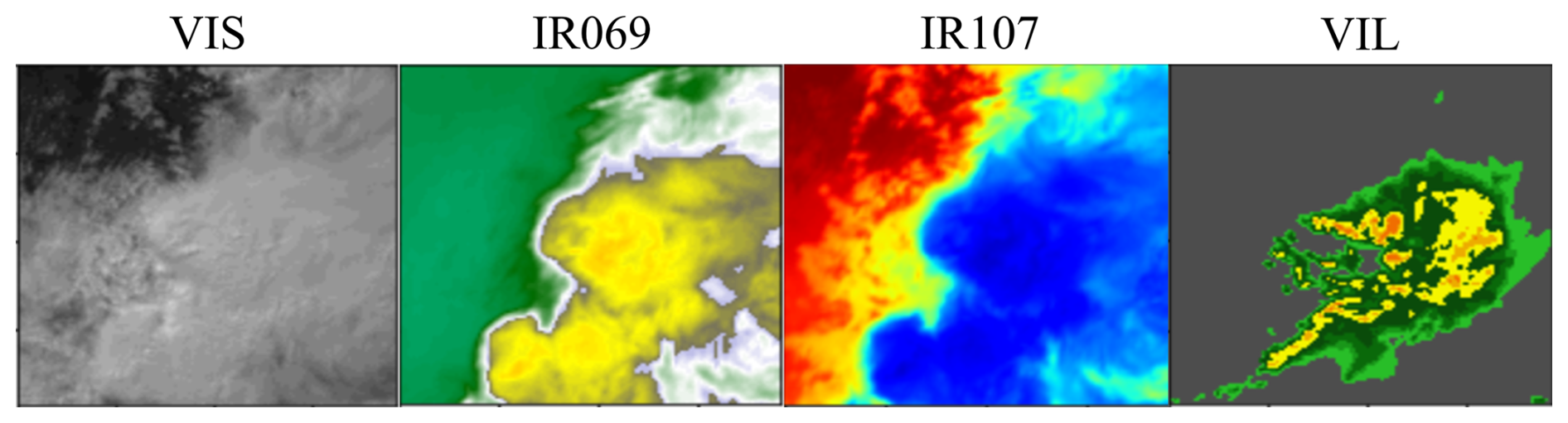
Figure 1 Visualization of various variables in the SEVIR (Storm Event Imager) dataset. VIL, IR107, VIS, and IR069 represent the radar vertical liquid water content, the satellite infrared longwave window, the visible satellite imagery, and the satellite mid-level water vapor, respectively. Among them, VIL represents precipitation data, while VIS, IR107 and IR069 serve as additional meteorological information.

As precipitation datasets now encompass longer temporal sequences, Transformer-based architectures have been introduced to address the limitations of CNNs in modeling temporal dependencies and the gradient vanishing issues inherent in RNNs (Piran et al., 2024). Notable examples include the MetNet (Sønderby et al., 2020) and Earthformer (Gao et al., 2022a) models, which have demonstrated enhanced predictive accuracy. Despite their superiority in handling general spatio-temporal sequences, these models struggle to reliably forecast moderate-to-intense precipitation events as prediction horizons extend.

Although current precipitation forecasting methods account for spatio-temporal features, the nonlinear characteristics and causal spatio-temporal relationships embedded in high-dimensional meteorological variables within historical observational data remain underutilized. This oversight significantly constrains model robustness and accuracy in precipitation prediction. From the perspective of chaotic dynamics, the Spatio-Temporal Information Transformation (STI) equations (Tao et al., 2023), derived from the delay embedding theorem (Jaurigue et al., 2025), provide a rigorous mathematical framework to simulate such atmospheric spatio-temporal dependencies. In time-series forecasting, prior studies have leveraged STI equations to model atmospheric dynamics – for instance, reservoir computing networks have employed semi-linear STI transformations to enhance feature representation (Chen et al., 2020b). However, the iterative solution of these semi-linear STI equations tends to accumulate errors and degrade predictive accuracy, and analogous methodologies remain scarce in computer vision. To bridge this gap, we propose a Spatio-Temporal Information-Dual Encoder-Decoder Network (STI-DEDN) that enables a more accurate approximate of STI equations inspired by the inherent conjugate duality of the STI equations. This framework explicitly resolves the spatio-temporal causal relationships between multivariate meteorological factors and precipitation dynamics. Crucially, it converts high-dimensional spatial meteorological features into temporal projections of future precipitation variables (Fig. 2a), thereby improving prediction robustness. Furthermore, we design an adaptive weighted gradient loss (ADGLoss) function to penalize underestimation biases in precipitation intensity. This loss function dynamically adjusts error gradients based on rainfall magnitude, effectively mitigating the precipitation underestimation and prediction ambiguity issue that models face as prediction time extends, while preserving the fine-scale precipitation structures. In addition, due to the particularity of VIL variables in the experimental dataset, all experiments in our paper are VIL intensity forecasts. However, this does not mean that our method cannot achieve excellent performance on real precipitation data. To validate this, we conducted additional experiments on the MeteoNet dataset containing real precipitation measurements. The results demonstrate that our method also achieves promising performance on real-world precipitation data. Consequently, in subsequent chapters, we use precipitation forecasts as an approximation for VIL forecasting.

Our principal contributions are threefold:

• Aiming at the prediction inaccuracies caused by existing STI equation solvers and the limitations of short-term data in forecasting short-duration heavy precipitation, we have established a novel dual encoder-decoder neural network that enables approximation of the STI equations and robust nonlinear mapping of high-dimensional meteorological and VIL precipitation variables.

• To improve the issue of precipitation underestimation in heavy rainfall areas and blurred predictions caused by the error amplification of existing precipitation models with extended prediction horizons, we propose an adaptive weighted gradient loss function that can effectively enhance the model's accuracy in spatiotemporal prediction tasks.

• Through comprehensive benchmarking experiments against state-of-the-art methods, we demonstrate a superior performance and generalizability of our framework. The experimental results show that the proposed method has more practical significance for VIL precipitation forecasting in medium and heavy VIL regions.

2 Related Work

2.1 Nowcasting Precipitation Based on Artificial Intelligence

ConvLSTM (Shi et al., 2015) introduced a groundbreaking approach to integrating CNNs and LSTM networks by incorporating convolutional operations within LSTM's gating mechanisms. This innovation marked the first successful application of deep learning to precipitation nowcasting, achieving breakthroughs in short-term forecasting accuracy. Building on ConvLSTM, Shi et al. (2015) further developed the TrajGRU model, which enhanced accuracy by combining temporal convolutional networks' sensitivity to spatiotemporal features with optical flow techniques for cloud motion simulation (Hui et al., 2021). Subsequent advancements include Wang et al. (2017)'s PredRNN, which employs Spatio-Temporal LSTMs to efficiently capture long-term dependencies in spatiotemporal sequences, significantly improving nowcasting precision. Seo et al. (2022) proposed the 3D-UNet model to predict high-resolution radar data from low-resolution inputs, while Ma et al. (2024) addressed prediction blurring via a DB-RNN to enhance high-frequency details. Wu et al. (2023) incorporated physical priors into the PastNet model, leveraging inherent inductive biases to boost prediction efficiency and effectiveness. Despite the robust feature learning capabilities of CNNs and RNNs, they still exhibit degraded performance when relying solely on short-term data and tend to underestimate intense precipitation events.

Transformer's self-attention mechanisms effectively address long-range dependency challenges in spatio-temporal sequence prediction, driving significant advancements in precipitation nowcasting. For instance, SmaAt-UNet (Trebing et al., 2021) integrates depthwise separable convolutions with scaled dot-product attention, substantially reducing the parameter count and computational overhead of traditional U-Net architectures. Earthformer (Gao et al., 2022a) enhances computational efficiency by hierarchically sharing global-local spatio-temporal features through axial attention blocks. Meanwhile, Rainformer (Bai et al., 2022) and MS-RadarFormer (Geng et al., 2024) employ tokenization of temporal frames combined with GFUs and convolutional attention layers, achieving notable improvements in predicting light-to-moderate precipitation events. Despite their superior performance, Transformer-based approaches struggle with forecasting heavy precipitation under short forecast horizons, and they suffer from quadratic computational complexity scaling with sequence length.

2.2 Time Series Prediction Based On Spatiotemporal Information Transformation Equation

In recent years, STI equations, derived from the delay embedding theorem, have demonstrated remarkable potential in regression-based forecasting. These equations establish bidirectional mappings between high-dimensional spatial data and future temporal dynamics of target variables, enabling mutual conversion of spatio-temporal information (Chen et al., 2020a). For instance, Chen et al. (2020b) proposed an ARNN that leverages reservoir computing (RC) architecture and semi-linear STI transformations to achieve accurate multi-step ahead predictions. Building on this, Tong et al. (Tong et al., 2023) introduced Reservoir-based Spatio-Temporal Information Transfer (RSIT), which integrates nonlinear time-series forecasting with critical point detection to develop a high-precision earthquake early warning framework. Furthermore, Peng et al. (2024) combined STI equations with self-supervised attention mechanisms to predict future values of target variables from high-dimensional inputs, achieving state-of-the-art robustness and accuracy in scenarios with sparse observational data, achieving superior and robust results. However, these methods are prone to cumulative errors during the iterative solution of STI mappings, and to date, no STI-based approach has been applied in the precipitation forecasting domain.

3 Method

3.1 Precipitation Prediction Based on STI

Conventional precipitation forecasting approaches have faced challenges in effectively leveraging spatio-temporal patterns embedded within meteorological systems. Drawing upon the theoretical framework of the STI equations, this study proposes a novel approach for precipitation forecasting that enables simultaneous spatiotemporal feature fusion within atmospheric phase-space dynamics. As shown in Fig. 2a, we define historical observational data of different meteorological variables in the atmospheric system as Z_n. It is called a non-delayed embedding attractor in n-dimensional space. In the original STI equations, these are represented as a one-dimensional vector ${\mathit{Z}}^t=\left(z_{\mathrm{1}}^t,z_{\mathrm{2}}^t,\mathrm{\cdots },z_n^t\right)$, where $t\in \left\{\mathrm{1},\mathrm{2},\mathrm{\cdots },m\right\}$, denotes m historical time steps. In this work, Z^t specifically refers to radar echo image frames of various meteorological factors recorded by radar sensors at time t. According to the delay embedding theorem, the corresponding delayed-embedded precipitation variable sequence is denoted as ${\mathbf{Y}}^t=\left(y^t,y^{t+\mathrm{1}},\mathrm{\cdots },y^{t+e-\mathrm{1}}\right)$, where the parameter e indicates the number of future image frames to predict. Separately, we express the historical observation spatiotemporal data of different meteorological variables input to the model in matrix form, and the representation of Z^t is as follows:

$$\begin{array}{}\text{(1)}& \mathbf{Z}=\left[Z^{\mathrm{1}},Z^{\mathrm{2}},\mathrm{\dots },Z^m\right]={\left[\begin{array}{cccc}{z}_{\mathrm{1}}^{\mathrm{1}}& z_{\mathrm{1}}^{\mathrm{2}}& \mathrm{\cdots }& z_{\mathrm{1}}^m\\ z_{\mathrm{2}}^{\mathrm{1}}& z_{\mathrm{2}}^{\mathrm{2}}& \mathrm{\cdots }& z_{\mathrm{2}}^m\\ \mathrm{⋮}& \mathrm{⋮}& \mathrm{\ddots }& \mathrm{⋮}\\ z_n^{\mathrm{1}}& z_n^{\mathrm{2}}& \mathrm{\cdots }& z_n^m\end{array}\right]}_{n\times m}\end{array}$$

where n is the number of variables in the atmospheric space system, and m is the observation length of the historical observation image sequence. In addition, its Y^t expression after delayed embedding is as follows:

$$\begin{array}{}\text{(2)}& \mathbf{Y}={\left[\begin{array}{cccc}{y}^{\mathrm{1}}& y^{\mathrm{2}}& \mathrm{\cdots }& y^m\\ y^{\mathrm{2}}& y^{\mathrm{3}}& \mathrm{\cdots }& y^{m+\mathrm{1}}\\ \mathrm{⋮}& \mathrm{⋮}& \mathrm{\ddots }& \mathrm{⋮}\\ y^e& y^{e+\mathrm{1}}& \mathrm{\cdots }& y^{m+e-\mathrm{1}}\end{array}\right]}_{e\times m}\end{array}$$

where Y^t is the delay embedding matrix with dimension e×m, and e is the number of future image frames of the precipitation variable to be predicted.

In the lower right corner of the delay embedding matrix Y, the sequence $(y^{m+\mathrm{1}},y^{m+\mathrm{2}},\mathrm{\cdots },y^{m+e-\mathrm{1}})$ of the target variable after the time point m are future image frames that need to be predicted. Through this transformation, a substantial amount of spatial variables $\mathit{\{}{Z}_{\mathrm{1}},Z_{\mathrm{2}},\mathrm{\dots },Z_n\mathit{\}}$ can be utilized to enrich the temporal information of the target variable $(y^{m+\mathrm{1}},y^{m+\mathrm{2}},\mathrm{\cdots },y^{m+e-\mathrm{1}})$ in the low-dimensional space via the delayed embedding process. While the generalized delay theorem theoretically supports multi-variable forecasting, the current implementation focuses on single-variable spatio-temporal information transformation for precipitation, as shown in Eq. (3).

$$\begin{array}{}\text{(3)}& \left\{\begin{array}{l}F\left([Z^{t-m},Z^{t-m+\mathrm{1}},\mathrm{\cdots },Z^t]\right)={\mathbf{Y}}^t\\ F^{-\mathrm{1}}\left({\mathbf{Y}}^t\right)=[{\widehat{Z}}^{t-m},{\widehat{Z}}^{t-m+\mathrm{1}},\mathrm{\cdots },{\widehat{Z}}^t]\end{array}\right.\end{array}$$

The traditional process of realizing STI transformation needs to iteratively solve the STI transformation equation. In this process, the computational complexity is high, and the cumulative error is large. To overcome these limitations, we leverage the end-to-end automated learning capabilities of deep learning to replace equation-solving procedures, which has a positive effect on the improvement of predictive robustness. Then the neural networks model used to fit the nonlinear map F becomes the key to the transformation from the known spatial information to the future target variable time information.

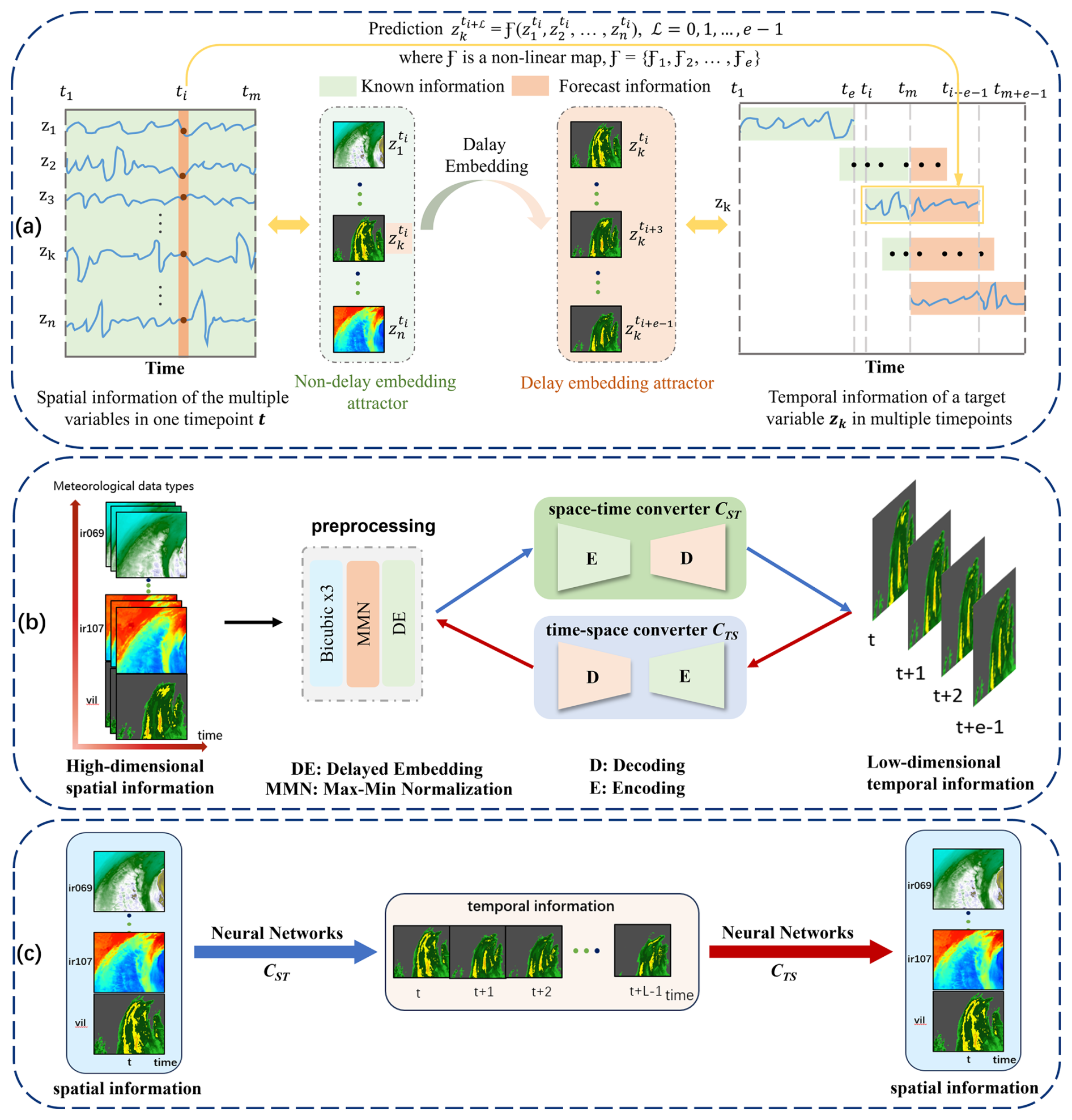
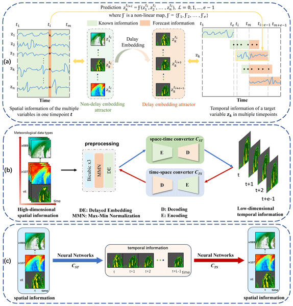
Figure 2 Schematic diagram of STI-DEDN. Panel (a) illustrates the transformation of the target variable z_k into a delayed embedding attractor using the delay embedding theorem, where the attractor exhibits a conjugate relationship with the non-delayed embedding attractor. The two attractors are connected through a nonlinear function ℱ, which maps the known spatial variable information to the temporal information of the unknown target variable z_k. The future values of z_k are represented as $z_k^{t_{i+\mathcal{L}}}=\mathcal{F}(z_{\mathrm{1}}^{t_i},z_{\mathrm{2}}^{t_i},\mathrm{\dots },z_n^{t_i}),\mathcal{L}=\mathrm{0},\mathrm{1},\mathrm{\dots },e-\mathrm{1}$. Therefore, the key to predicting z_k lies in fitting the nonlinear function ℱ. Panel (b) demonstrates the overall training architecture of our proposed STI-DEDN, which mainly includes a space-time converter and a time-space converter, them are implemented using the same neural architecture. Panel (c) mainly illustrates the information flow process of STI-DEDN, the main STI equation corresponds to C_ST, and the conjugate STI equation corresponds to C_TS.

3.2 Overall Network Framework Based on STI

According to the structural characteristics of the conjugate-dual of the spatiotemporal information transformation equation, we propose the Spatio-Temporal Information-Dual Encoder-Decoder Network (STI-DEDN). This architecture builds upon ConvLSTM as its backbone, which is adapted to a dual-training framework to efficiently approximate the nonlinear STI equations. The dual-based training method leverages the inherent properties of the STI conjugate equation to establish mutual learning between two interdependent prediction tasks (Chen et al., 2020b). This synergistic framework enhances model robustness through cross-task knowledge transfer, effectively mitigating prediction overfitting risks while strengthening the model's generalization capability under varying meteorological conditions.

Table 1 Detailed architectural configuration of STI-DEDN.

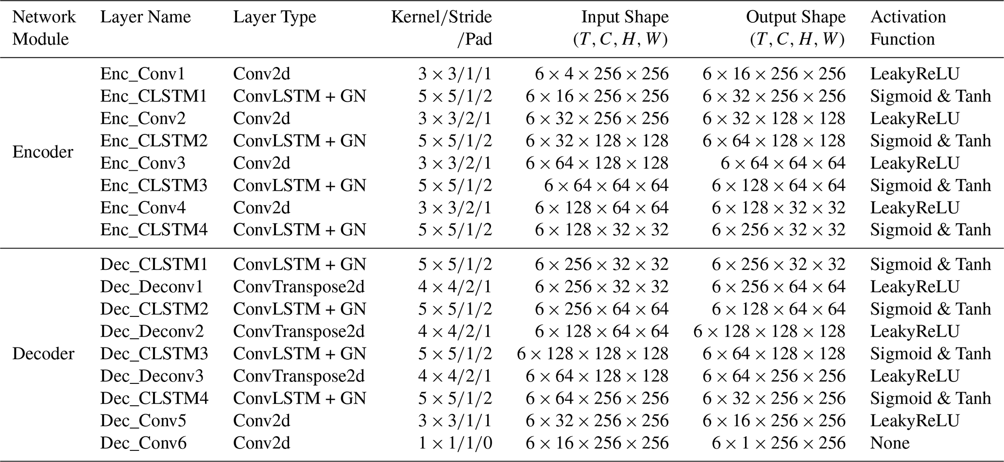
Note: GN stands for GroupNorm. The channel size (C) in the output shape of ConvLSTM layers represents the hidden state feature dimension.

As shown in Fig. 2b, the STI-DEDN architecture comprises three primary components: the data preprocessing module, the spatio-temporal converter C_ST, and the temporal-spatio converter C_TS. To solve the problem of inconsistent spatial and temporal resolutions between meteorological data, we use the data preprocessing module to process meteorological data into data with consistent resolution, which can eliminate potential errors caused by resolution between meteorological data from different sources. Finally, the input data is adjusted to a fixed form that conforms to the STI equation according to the delay embedding theorem, which is convenient for the effective extraction of subsequent spatiotemporal features. In addition, the spatio-temporal converter C_ST and the temporal-spatio converter C_TS for processing spatiotemporal information belong to the encoding-decoding prediction architecture, and the modules of the encoder and decoder are realized by the multi-layer adapted ConvLSTM model. The encoder and decoder use the interaction of multi-layer convolution and LSTM to capture the potential order and potential spatiotemporal information between the observation data of the input m time points.

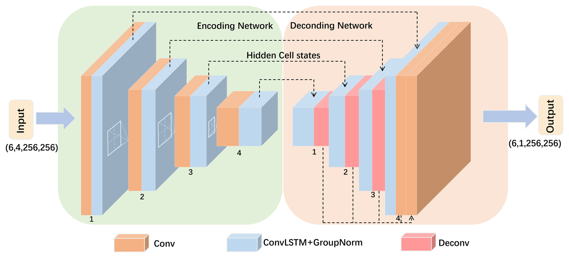
The spatio-temporal information flow in the STI-DEDN architecture is illustrated in Fig. 2c. The spatial-temporal converter C_ST transforms input spatial information into temporal information (forward process), while the temporal-spatial converter C_TS converts temporal information back into spatial information (reverse process). The detailed implementations of Encoding and Decoding for both processes are shown in Fig. 3. Specifically, in the STI-DEDN architecture, CNNs extract hierarchical spatial features from input tensors, while RNNs convert these features into hidden states encoding multi-scale temporal dependencies. This dual-stream mechanism collectively extracts latent spatiotemporal patterns. The decoder then employs transposed convolutions to project high-level features back to the original input space, enabling precipitation prediction. By stacking multiple CNN+RNN layers, the architecture comprehensively captures intrinsic relationships between high-dimensional spatiotemporal data and precipitation patterns and can play a positive role in approximating the STI equation. The main formula of this structure is as follows:

$$\begin{array}{}\text{(4)}& C_{\mathrm{TS}}\left(C_{\mathrm{ST}}\right(z\left)\right)\approx z\end{array}$$

In this study, our ConvLSTM architecture largely follows Shi et al. (2015)'s design, with all convolutional layers using 3×3 kernels. Each successive convolutional layer halves the spatial dimensions of the input while doubling the number of hidden features. We incorporate GroupNorm into Shi et al. (2015)'s ConvLSTM to reduce feature scale discrepancies, thereby making model training less dependent on batch size, lowering hardware requirements, and enhancing the model's ability to capture inter-feature relationships. To mitigate vanishing gradients and information loss during precipitation reconstruction, residual connections are added after GroupNorm layers to stabilize training. The remaining ConvLSTM parameters are initialized based on Shi et al. (2015)'s prior work, with hyperparameter optimization conducted to improve predictive performance. The detailed parameter settings for all layers of the module are shown in Table 1.

Figure 3 Implementation of Encoding Network and Decoding Predictive Network.

3.3 Loss Function

A common problem in precipitation forecasting is that the spatial distribution of precipitation data exhibits regional heavy precipitation characteristics. Conventional regression-based loss functions, such as MSE (Mean Squared Error) and MAE (Mean Absolute Error), focus on minimizing pixel-wise numerical discrepancies between predictions and the ground truth. While they demonstrate competence in modeling continuous, homogeneous precipitation fields, they exhibit fundamental limitations in reconstructing the regional spatial feature details which reconcile the non-stationary patterns between heavy and light precipitation inadequately. This results in a uniform distribution of errors, causing models to overpredict rainfall in light precipitation areas and underpredict it in heavy precipitation zones. To address this, we apply the Gradient Difference Loss (GDLoss) function (Byeon et al., 2018), defined as the Equation:

$$\begin{array}{}\text{(5)}& \begin{array}{rl}\mathrm{GDLoss}& =\sum _{i=\mathrm{1}}^m\sum _{j=\mathrm{1}}^n({\left|\Vert X_{i,j}-X_{i-\mathrm{1},j}\Vert -\Vert Y_{i,j}-Y_{i-\mathrm{1},j}\Vert \right|}^{\mathit{\beta }}\\ & +{\left|\Vert X_{i,j-\mathrm{1}}-X_{i,j}\Vert -\Vert Y_{i,j-\mathrm{1}}-Y_{i,j}\Vert \right|}^{\mathit{\beta }})\end{array}\end{array}$$

where X_i,j and Y_i,j represent the pixel values of the predicted image and the target image at position (i,j), $X_{i,j}-X_{i-\mathrm{1},j}$ represents the layer change rate of the predicted image in the horizontal direction, $Y_{i,j-\mathrm{1}}-Y_{i,j}$ represents the layer change rate of the target image in the vertical direction, where β is an integer greater than or equal to 1, usually 1 or 2, used to adjust the sensitivity of the loss.

The GDLoss quantifies spatial precipitation variations by comparing gradients between predicted and the target radar echo maps. It emphasizes the differences between the horizontal and vertical gradients of precipitation intensity, thereby better capturing spatial transitions in complex precipitation patterns. When the local gradient of the predicted field is smaller than the corresponding gradient of the ground truth field, GDLoss penalizes such deviations, ensuring alignment between predicted and ground-truth precipitation features during training, thus restoring the clarity of predictions. On the basis of GDLoss and MAELoss, we propose an adaptive-weighted gradient loss(ADGLoss) function, formulated as Eq. (8):

$$\begin{array}{}\text{(6)}& {\displaystyle }\mathrm{MAELoss}={\displaystyle \frac{\mathrm{1}}{n}}\sum _{i=\mathrm{1}}^n|x_i-y_i|\text{(7)}& {\displaystyle }\mathit{\alpha }=\left\{\begin{array}{ll}\frac{{\sum }_{i=\mathrm{1}}^n{y}_i^{\mathrm{2}}}{{\sum }_{i=\mathrm{1}}^n{x}_i^{\mathrm{2}}+\mathit{ϵ}},& y_i\ge x_i\\ \frac{{\sum }_{i=\mathrm{1}}^n{x}_i^{\mathrm{2}}}{{\sum }_{i=\mathrm{1}}^n{y}_i^{\mathrm{2}}+\mathit{ϵ}},& x_i>y_i\end{array}\right.\text{(8)}& {\displaystyle }\mathrm{ADGLoss}=\mathit{\alpha }\cdot \mathrm{MAELoss}+\mathrm{GDLoss}\end{array}$$

where x_i represents the model prediction result, y_i represents the true value, and n represents the number of samples. Combining the MAE and GDL loss functions allows the model not only to leverage MAE for maintaining balanced accuracy in overall forecasts but also to enhance edge information through GDL while addressing the issue of prediction ambiguity in complex precipitation regions. The parameter α is a dynamic adaptive weighting factor for layer-wise adjustments, improving the model's sensitivity to heavy precipitation forecasts. ϵ is a tiny positive constant introduced to prevent division-by-zero errors in extreme cases, although such all-zero outputs were virtually absent in our experiments. When the model underestimates or overestimates precipitation in complex precipitation regions, α exceeds 1, which increases the loss value, enhances the capability of MAE loss to capture global high-frequency precipitation patterns, and improves the prediction accuracy of heavy precipitation areas, thereby reducing the precipitation underestimation issue in precipitation forecasting tasks. Specifically, the weighting factors α is not a fixed hyperparameter, but is calculated dynamically during training. For each training batch, the model first performs forward pass to generate the prediction x_i. Then it uses Eq. (7) to calculate the ratio weight between the predicted image x_i and ground truth y_i. α then acts on the MAE loss component in backpropagation. This mechanism ensures that the model adapts to underestimating and overestimating precipitation, forcing the model to pay more attention to the absolute error between the prediction and the true value.

4 Experiments Basis

4.1 Dataset

All experiments in this study utilize the multimodal radar dataset SEVIR (Storm Event Imagery) (Veillette et al., 2020), collected by the Massachusetts Institute of Technology (MIT) and publicly available, which exhibits temporal and spatial alignment. The SEVIR dataset contains approximately 10 000 weather events (including storms and random weather patterns) across the continental United States (CONUS) from 2017 to 2019. These events comprise high-spatiotemporal-resolution radar image data captured by the GOES-16 geostationary satellite and the NEXRAD weather radar, respectively. Each event consists of a 4 h radar image sequence with a temporal resolution of 5 min and a spatial resolution of 0.01° for precipitation data (equivalent to a 1 km × 1 km horizontal resolution), providing detailed regional meteorological information. By integrating heterogeneous sensing modalities into a unified framework, avoiding the problem that traditional radar and meteorological satellite datasets are too large to process and calculate data in batches. The dataset includes four satellite sensor types and covers five distinct data categories, as summarized in Table 2 and Fig. 1.

Table 2 The variable information of dataset.

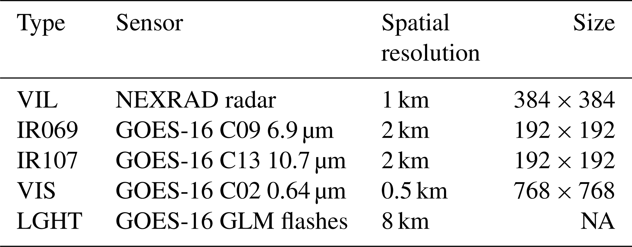
NA – not available.

Table 3 Comparison of results with and without interpolation for STI-DEDN on the SEVIR test set. NOP represents the number of parameters of the model, and ET represents the training time of the model for each round of epoch.

In this study, we excluded lightning data and selected four other data types for experimentation. Lightning data is stored as site events (precise spatiotemporal coordinates), while the other modalities (IR, VIS, VIL) are all rasterized radar images. Lightning events that cannot be captured by meteorological stations are set as no-lightning supervision information. Converting sparse point events into raster format requires additional interpolation and aggregation methods, which inevitably introduce artificial patterns and noise, deviating from the true physical process. This spatiotemporal mismatch can interfere with model learning and reduce the reliability of predictions. Lightning is a byproduct of strong convective activity, and strong convective activity does not necessarily accompany lightning events (Zhao et al., 2025). Moreover, the contribution of lightning data to precipitation forecasting is very low (Yang and Li, 2024). For VIL precipitation data, abnormal echo values may occur in radar image records due to factors such as mountainous terrain. Therefore, We excluded weather events with less than 4 h of weather duration and missing time points in weather events, accounting for 3 % of total events. In addition to storing precipitation data, we employed a mask matrix to identify valid and invalid data points, where 1 denotes normal values and 0 denotes anomalous values in the matrix. Using the transformation formula proposed by Veillette et al. (2020), we converted radar recorded values to physical VIL units (kg m⁻²). The formula reveals a positive correlation between VIL pixel values and actual precipitation measurements, as expressed below:

$$\begin{array}{}\text{(9)}& \mathrm{VIL}\left(x\right)=\left\{\begin{array}{ll}\mathrm{0},& x\le \mathrm{5},\\ \frac{x-\mathrm{2}}{\mathrm{90.66}},& \mathrm{5}<x\le \mathrm{18},\\ e^{\frac{x-\mathrm{83.9}}{\mathrm{38.9}}},& \mathrm{18}<x\le \mathrm{254}.\end{array}\right.\end{array}$$

To resolve spatial resolution inconsistencies among data modalities in the SEVIR dataset, we uniformly resampled all data types via bicubic interpolation, standardizing their dimensions to 256 × 256 (with a spatial resolution of 1.5 km) to reduce model training complexity. Although bicubic interpolation may introduce slight artifacts or smooth fine-scale features in the data, the original SEVIR dataset has already been aligned in spatial location and time. Our interpolation only changes the pixel resolution and does not affect the spatial patterns between different variables. Moreover, bicubic interpolation can balance computational efficiency, producing smoother results than nearest-neighbor or bilinear methods, which helps maintain the continuity of meteorological fields. Additionally, we conducted extra experiments to retrain and test the model without interpolation at the original resolution. As shown in Table 3, there was almost no difference. Given the significant numerical discrepancies between individual radar recordings, extrapolation models tend to suffer from poor convergence. Therefore, we normalized the initial radar precipitation values to the range of [0, 1] (Tan et al., 2024). Additionally, to assign precipitation values to areas without radar echoes, we set such values to 0.

Finally, the dataset of 10 000 weather events was allocated to training, validation, and test sets. Following random shuffling, the first 8000 events were assigned to the training set, events 8000–9000 comprised the validation set, and the remaining 1000 events formed the test set. In addition, due to the 5 min resolution of the precipitation data, consecutive 5 min frames exhibit minimal variation. To make the precipitation map of each frame have greater differences, we perform skip sampling (every 10 min) for four sensor types, that is, the period is 10 min, and then we use the 60 min meteorological data to predict the precipitation information over the next 60 to 180 min horizon. In addition, we used the MeoteoNet dataset in the additional experiment, which contains multiple types of meteorological elements such as radar precipitation observation data. The temporal resolution of the precipitation data is 5 min, and the spatial resolution is 1 km. We processed the dataset and verified that the classification criteria were consistent with the SEVIR dataset.

Table 4 Performance evaluation metrics used in this study.

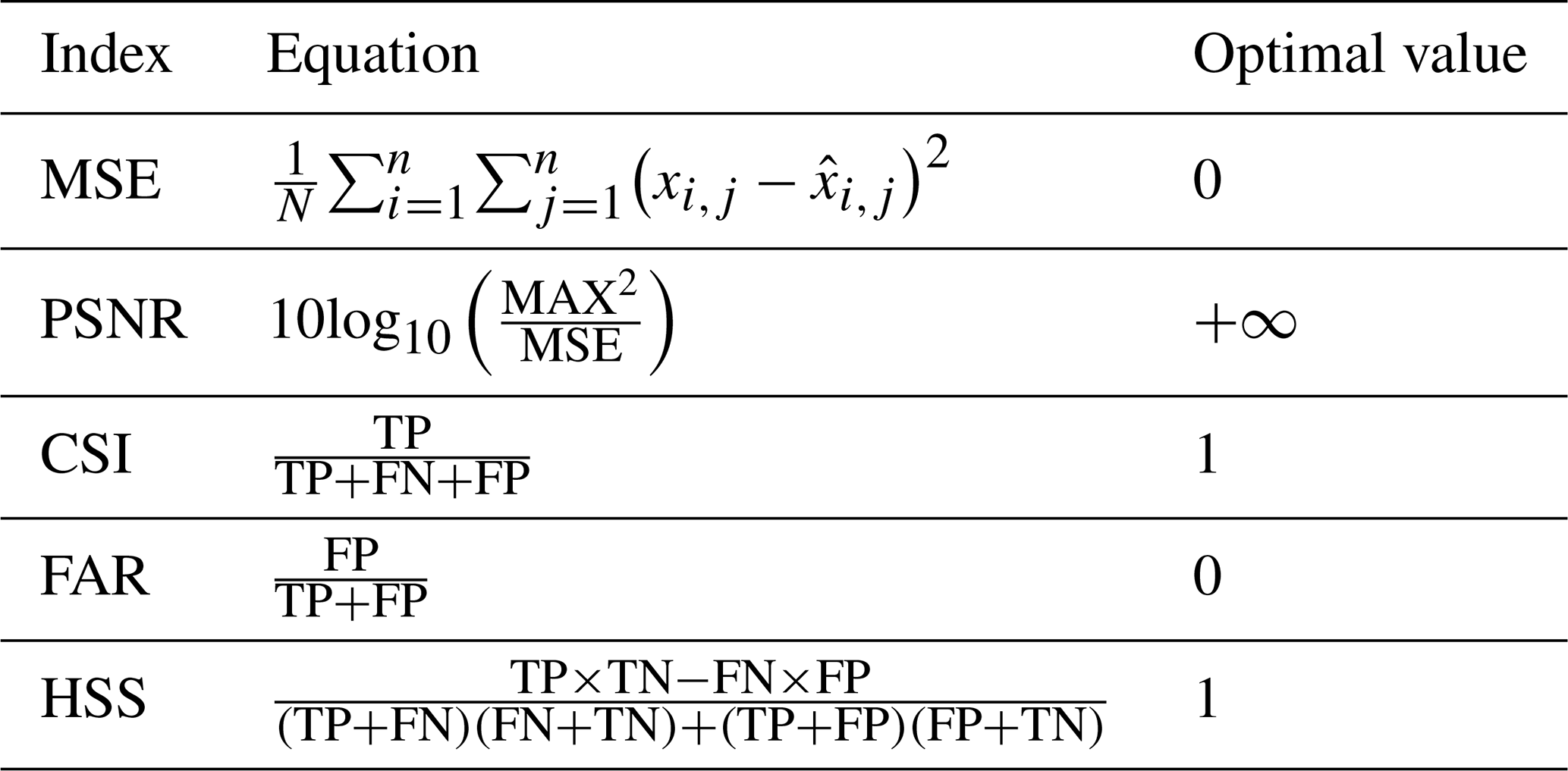
Note: N is the total number of outputs, x_i,j represents the size of the true value of image at weather radar image position (i,j), and ${\widehat{x}}_{i,j}$ represents the size of the predicted value at the same position; MAX represents the maximum value of all pixel values; y_i,j represents the size of the predicted value of weather radar echo image position (i,j); true positive (TP) represents prediction = 1, true value= 1; false negative (FN) represents prediction = 0, true value = 1; false positive (FP) represents prediction = 1, true value = 0; true negative (TN) represents prediction = 0, true value = 0.

4.2 Evaluation Metrics

In this study, we quantitatively evaluate our proposed STI-DEDN training framework using evaluation metrics from both the image domain of computer vision and the field of meteorological science, as presented in Table 4. Specifically, we employ the mean square error (MSE) (Hodson et al., 2021) as a primary evaluation metric, which measures the mean deviation between the predicted pixel values and the true pixel values. This metric allows us to assess the overall pixel value discrepancy between the predicted image and the actual image. Additionally, we utilize the peak signal-to-noise ratio (PSNR) (Cheon et al., 2021) to analyze the ratio of signal to noise between images, thereby evaluating the quality of the predicted image.

In the context of meteorological science, it is crucial to forecast various levels of precipitation accurately. To facilitate this, we establish indicator discrimination thresholds at [16, 74, 133, 160, 181, 219] based on the pixel values of the vertically integrated liquid (VIL). The corresponding true precipitation values are [0.15, 0.78, 3.53, 7.07, 12.14, 32.23] kg m⁻². Furthermore, we select the Critical Success Index (CSI) (Tan et al., 2024), False Alarm Rate (FAR) (Harnist et al., 2024), and Heidke Skill Score (HSS) (Ling et al., 2025) as additional metrics to evaluate the false alarm rate and accuracy of all methods employed for precipitation forecasting under varying threshold conditions.

Table 5 Comparison of computational efficiency during the inference phase across different methods. FPS denotes frames per second.

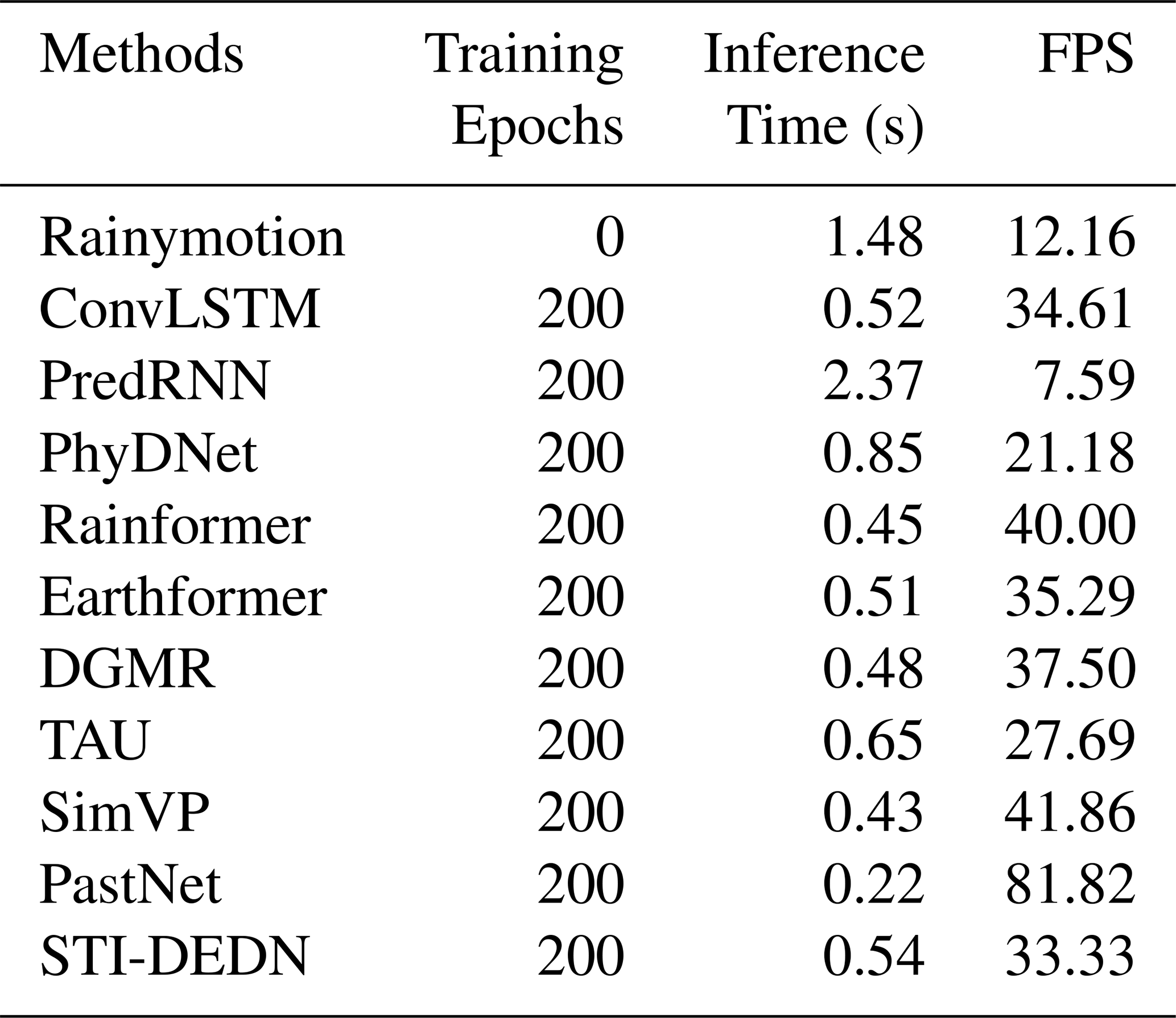
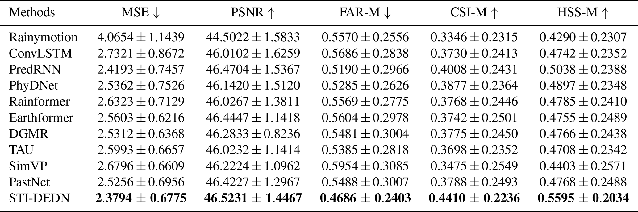
Table 6 Comparison of index results of each method under SEVIR test set, with the best results highlighted in bold.

4.3 Environment Setup

All code frameworks utilized in this study are based on the PyTorch design. The training and testing of the overall model were conducted on an Ubuntu 20.04 system. The CPU configuration employed is an Intel(R) Xeon(R) Gold 5218R CPU operating at 2.10 GHz, while the GPU hardware configuration consists of an NVIDIA GeForce RTX 3090, which features a video memory size of 24 GB. The parameters for the other comparison models used in the experiment are consistent with those specified in the official open-source code. The optimizer we employ is Adaptive Moment Estimation (AdamW) with decoupled weight decay. The learning rate is set to 0.0001, and the training step is configured to 200. The training batch size is set to 2. On a single NVIDIA GeForce RTX 3090 (24 GB) GPU card, the average training time per epoch is about 2.55 h, and the total training time for 100 epochs is about 255.55 h. For inference, the model takes approximately 0.54 s to process a radar sequence (18 frames), corresponding to an inference speed of about 34 frames per second. After each training iteration, we evaluate the model's performance on the validation set. In our experiments, all baseline models employed the same multi-modal inputs, preprocessing pipelines, and dataset partitioning criteria as STI-DEDN, ensuring a fair comparison without architectural modifications. Additionally, Table 5 summarizes the computational efficiency during the inference phase to demonstrate practical operational viability.

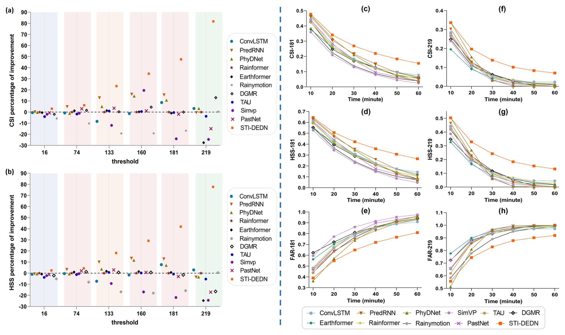
Figure 4 (a, b) scatter plots showing performance improvements at different measurement thresholds, using Rainformer as the baseline. Panels (c)–(h) show the time effect of each evaluation indicators of the model under the condition of high threshold precipitation.

Table 7 Comparison of index results of each method under MeoteoNet test set, with the best results highlighted in bold.

5 Experimental Results and Analysis

5.1 Overall Forecast Performances on Testing Data

5.1.1 Quantitative Evaluation of Overall Predictive Performance

To validate the quality and performance of our STI-DEDN model for high-resolution short-term precipitation forecasting, as well as to assess its applicability for short-term forecasting across different levels of precipitation. We compared our method with the optical flow method (Ayzel et al., 2019) based on radar echo extrapolation and several state-of-the-art methods in spatiotemporal forecasting, including ConvLSTM, PredRNN, PhyDNet (Guen and Thome, 2020), DGMR (Ravuri et al., 2021), Rainformer, Earthformer, SimVP, TAU (Tan et al., 2023), and PastNet. Since our model is RNN-based, comparisons with other RNN- and CNN-based approaches allow for a clear and direct evaluation of its forecasting capabilities, showing that STI-DEDN consistently outperforms these methods across key performance metrics. Furthermore, by comparing STI-DEDN with Transformer-based architectures, we can assess our model's ability to capture global contextual information relative to advanced attention mechanisms.

To ensure experimental accuracy in this study, we consistently selected models exhibiting minimal loss function values post-training across all methods, while performing evaluations and testing on an identical test set. Table`6 shows the one-hour forecast results of our method in comparison with the other methods on the SEVIR dataset. From the quantitative evaluation metrics presented in the above table, it is evident that the model proposed in this study demonstrates superior performance in short-term forecasting compared to other methods, with higher accuracy in the predicted precipitation images. In the foundational one-hour precipitation forecast, ConvLSTM and SimVP exhibit relatively MSE scores and relatively low PSNR scores. This indicates that the capabilities of CNN and RNN-based models in extracting precipitation information are comparatively weak. Furthermore, the Rainformer and Earthformer models both demonstrate higher MSE and lower PSNR values compared to the STI-DEDN model. This suggests that our proposed method outperforms Transformer-based methods in this context.

We calculated the average FAR, CSI, and HSS scores across all methods at the 60 min lead time. The approach demonstrated the lowest FAR-M value, reflecting its minimal false alarm rate. It achieved the highest CSI-M and HSS-M scores, demonstrating its superior forecasting performance and higher prediction accuracy. Specifically, for short-term forecasting, the STI-DEDN model surpassed PredRNN, which is the top-performing alternative, with improvements of 10.03 % in CSI-M, 11.07 % in HSS-M, and 9.71 % in FAR-M. Finally, Table 7 is an additional experiment on the MeteoNet dataset – a high-resolution meteorological dataset from France containing multi-source meteorological data including real radar precipitation observations with 5 min temporal resolution. This supplementary experiment was not part of our primary evaluation but served to validate STI-DEDN's effectiveness for real precipitation forecasting. The experiment uses one hour of radar precipitation observations as input to predict precipitation for the following hour. The experiment is compared with the traditional optical flow method Rainymotion, and the results show that STI-DEDN is still valid for real precipitation forecasting, which is an effective step for us to use real-world precipitation as a forecasting condition in future studies.

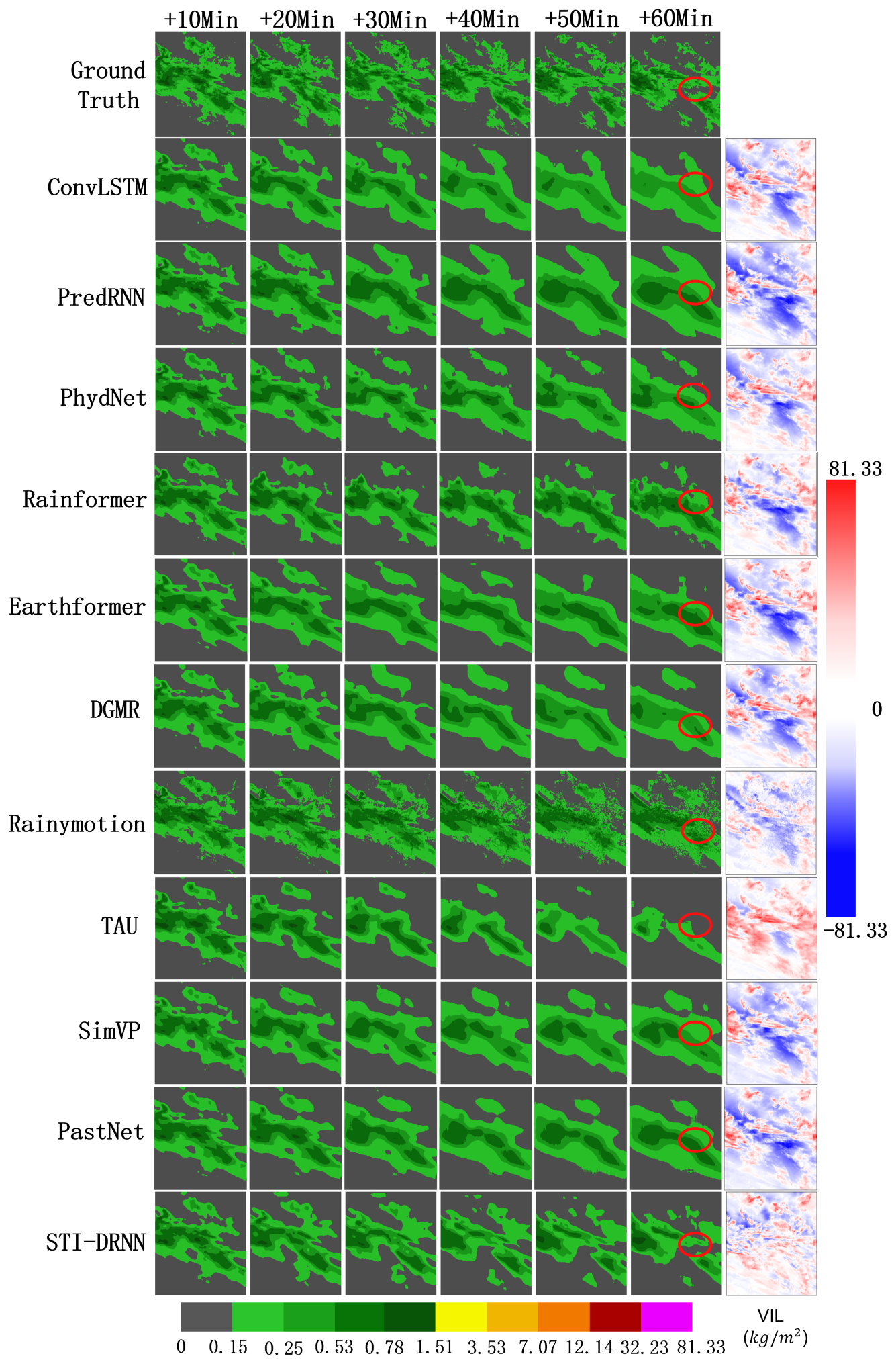
Figure 5 Visual precipitation maps and error heatmaps for all methods in common precipitation events.

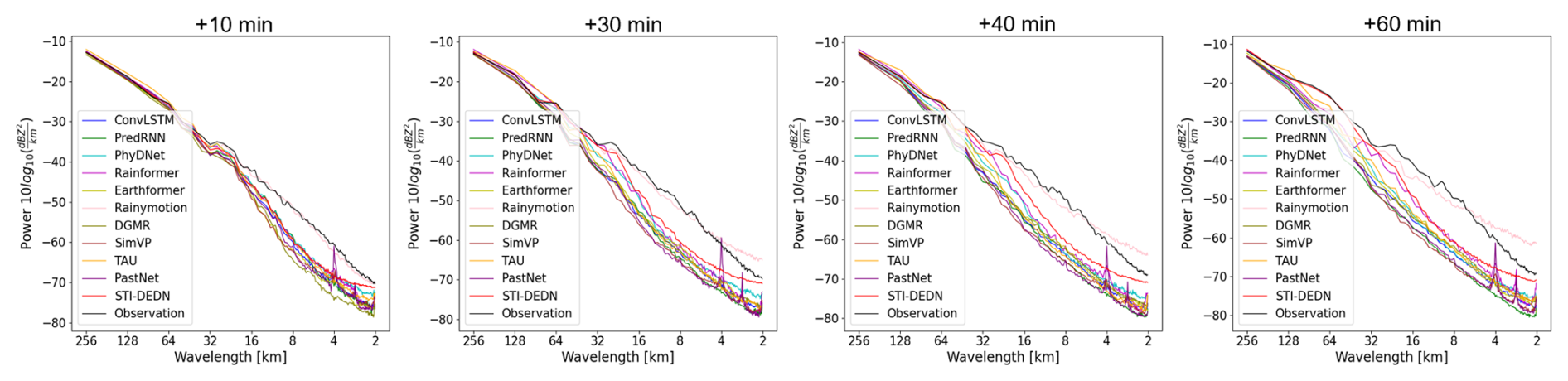
Figure 6 The radial mean power spectral densities (RAPSDs) for all methods in Case 1 were compared with the observed RAPSDs at 10, 30, 40, and 60 min lead times. The observed RAPSDs are shown as solid black lines.

5.1.2 Qualitative Evaluation Under Different Precipitation Thresholds

Generally, meteorology emphasizes model performance across varying precipitation thresholds and it is essential to assess effectiveness under different precipitation intensities for all methods. We achieved it with the scores of CSI and HSS, which are illustrated in Fig. 4a, b. Rainformer is used as the baseline and calculated the percentage improvements in the CSI and HSS scores of all other methods. The result demonstrates that our STI-DEDN method achieves consistent performance improvements over the Rainformer baseline across all thresholds, with enhancement values attaining their maximum levels at each measurement point. Notably, as the precipitation thresholds increase, the challenge of precipitation forecasting intensifies; however, the percentage improvements of our method exhibit a positive correlation with the precipitation thresholds. It suggests that the STI-DEDN model demonstrates particular efficacy in forecasting medium-to-high-intensity precipitation.

Based on the experimental analysis above, we conclude that our method achieves superior predictive performance for moderate to heavy precipitation of short-term forecasts. To further validate the STI-DEDN model's predictive accuracy specifically for moderate-to-heavy precipitation events, we plotted temporal performance analysis graphs at precipitation thresholds of 181 and 219, as illustrated in Fig. 4c–h. The figure demonstrates that extended forecast horizons correlate with amplified model uncertainty, resulting in progressive deterioration of predictive accuracy across all methodologies over time. As shown in the results, our STI-DEDN outperformed the other methods in all thresholds, demonstrating a less pronounced decline in predictive metrics. Notably, as the forecast horizon extends, the difference of performance between the STI-DEDN model and others becomes pronounced increasingly. And it means that this proposed approach is highly competitive in short-term prediction. When compared to the PredRNN model, which exhibits strong overall predictive capabilities among other models, our STI-DEDN model achieved a 27.77 % improvement in the CSI score at the threshold of 181 and an impressive 82.64 % improvement at the threshold of 219. Similarly, the HSS score improved by 25.75 % at the threshold of 181 and by 84.06 % at the threshold of 219.

5.2 Case Studies

To evaluate the warning capability of the STI-DEDN model in real-world precipitation scenarios, we randomly selected a range of test cases, encompassing routine rainfall occurrences and infrequent extreme precipitation phenomena. Error heatmaps were integrated into the visual analysis to quantitatively evaluate the model's prediction bias tendency. This heatmap compares the sixth predicted frame with the corresponding ground truth frame. In the heatmap, red regions indicate underestimation phenomena, while blue regions indicate overestimation phenomena.

5.2.1 Case 1: Evaluation of Common Precipitation Events

The first case is a large-scale conventional rainfall event across the continental United States. We believe it serves as a baseline for evaluating our model's forecasting performance under typical precipitation conditions. This is essential for establishing the reliability of our method in everyday scenarios. Figure 5 shows its visual prediction results. The green area of the ground truth shows very clearly the spatial distribution of precipitation intensity, and the precipitation range narrows over time progressively. Compared to other methods, STI-DEDN demonstrates higher accuracy in capturing both the spatial structure and temporal dynamics of precipitation distribution. Especially in the morphology and boundary part of the precipitation area (the area marked by the red circle in the figure), STI-DEDN shows better modeling ability of regional dynamic evolution than other methods. The error analysis shown on the figure's right side reveals that the STI-DEDN's red and blue regions display the lightest coloration, indicating lower error magnitudes. Furthermore, the error sources across all methods are concentrated along precipitation boundaries predominantly, where precipitation exhibits significant spatial-temporal variability that challenges modeling efforts. Despite this, the overall error produced by the STI-DEDN remains relatively small and is distributed more uniformly, indicating that our method possesses stability in spatiotemporal predictions. This stability effectively addresses the issues of overestimation and underestimation of precipitation, thereby enhancing the reliability of the forecasts.

The Radial Average Power Spectral Density (RAPSD) (Ayzel et al., 2020) is utilized to assess the smoothness and ambiguity of precipitation fields across different spatial scales, where lower spectral power values correspond to more smoothness and ambiguity in precipitation patterns. Figure 6 presents the RAPSD curves for all methods at forecast lead times of 10, 30, 40, and 60 min. The STI-DEDN outperforms these state-of-the-art methods in predictive performance across various spatial scales. As illustrated in the figure, within the range of all lead times, the STI-DEDN's predictions in the large wavelength range (> 64 km) nearly overlap with the true values. In the medium to small scale range (< 32 km), all methods exhibit a significant loss in power spectral density; however, the blurring effect produced by the STI-DEDN is lower than that of the existing deep learning methods. It is worth noting that deep learning models inherently possess stochasticity, and some degree of fluctuation is normal when forecasting highly non-linear precipitation, but PastNet's architectural traits make these artifacts more pronounced at small scales. Overall, the results indicate that the STI-DEDN is capable of providing robust technical support for multi-scale forecasting tasks in the context of conventional precipitation events. This demonstrates the model's effectiveness in maintaining accuracy and reliability across varying spatial resolutions, thereby enhancing the overall quality of precipitation forecasts.

5.2.2 Case 2: Evaluation of Extreme Precipitation Events

The second case involves a localized heavy precipitation event, which highlights our model's capability in predicting severe weather events. From Fig. 7, all methods experience a progressive loss of predictive detail in precipitation forecasting as forecast time extends. Notably, the PhydNet method exhibits the most severe information loss concerning precipitation events. All methods exhibit a higher incidence of underestimation or overestimation when compared to actual precipitation imagery, although they achieve foundational predictive capabilities. They exhibit larger errors in precipitation spatial distribution and general morphology within darker regions described as yellow and above particularly, where predictions appear blurred and displaced. In contrast, although the STI-DEDN model inevitably still encounters some issues of underestimation and overestimation, its predictive results are significantly closer to the actual values. Moreover, the STI-DEDN model demonstrates reduced overestimation and underestimation, evidencing its capacity to capture intricate spatiotemporal information within the data effectively. The demonstrated efficacy in spatiotemporal data transformation indicates the superior spatiotemporal modeling of STI-DEDN, compared to alternative approaches in processing medium- to high-intensity precipitation events.

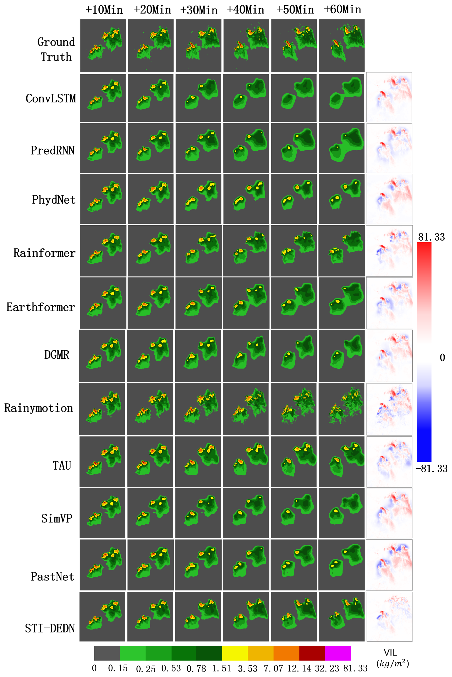
Figure 7 Visual precipitation maps and error heatmaps for all methods in Case 2.

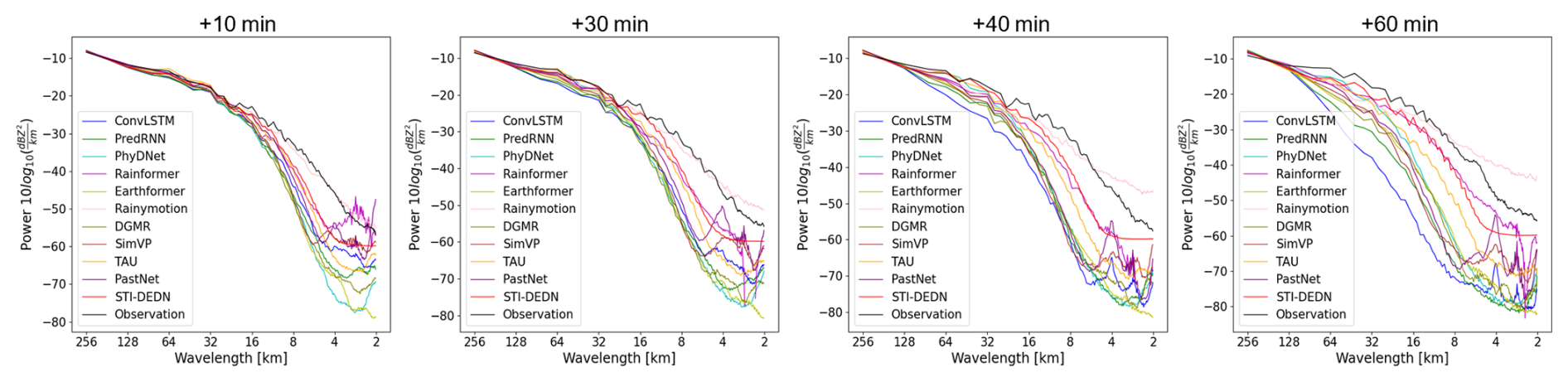
Figure 8 At the lead times of 10, 30, 40, and 60 min, the RAPSD curves at different precipitation thresholds for all methods in Case 2 were obtained.

Figure 8 presents the PSD scores of all methods at different spatial scales. As the forecast lead time extends, the STI-DEDN model maintains optimal accuracy in predicting weather events across varying precipitation thresholds. Furthermore, in this case study, the power spectral curve of the STI-DEDN model closely aligns with the true values within the wavelength range of 64 to 256 km, whereas other models begin to deviate from the true values at a wavelength of 128 km. This observation indicates that the STI-DEDN model provides information that is nearly consistent with the ground truth over large spatial scales. In contrast, at smaller spatial scales, all methods yield lower PSD scores, which appear to be independent of the forecast lead time. This suggests that deep learning methods tend to introduce smoother and more ambiguous precipitation fields at smaller scales; however, the blurring effect of the STI-DEDN model is comparatively lower than that of the other methods. Overall, STI-DEDN is more suitable for forecasting precipitation under large-scale spatial conditions.

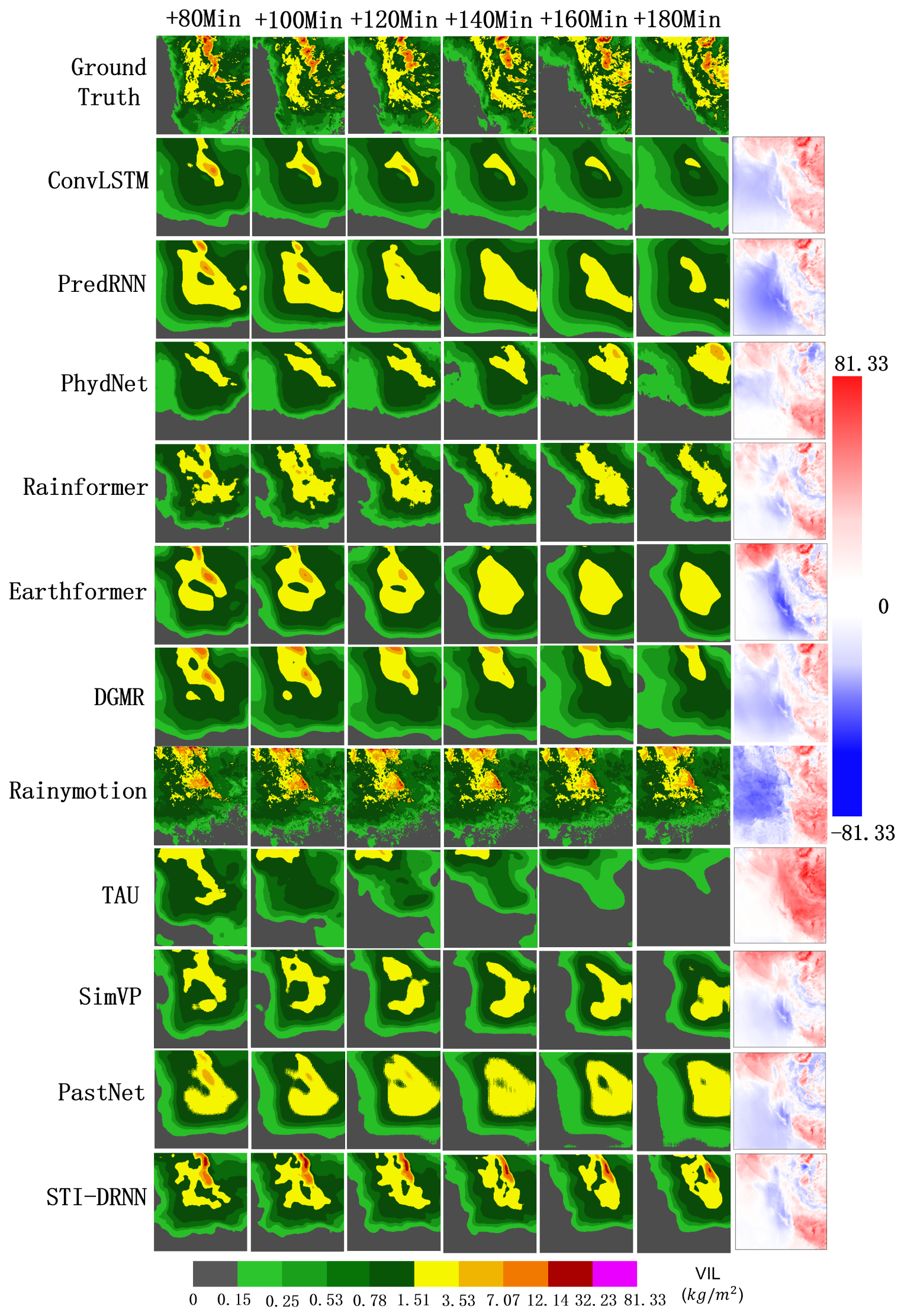
Figure 9 Visualization of precipitation maps and error heatmaps for all methods in the long-term experiment of Case 3.

Table 8 Comparison of the visual index results for 2 and 3 h forecasts of each method under the SEVIR test set, with the best results highlighted in bold.

5.3 Results of Long-Term Forecasting

Furthermore, to emphasize the long-term forecasting capabilities of all methods, we performed an extended forecast lasting three hours, utilizing one hour of input data to predict precipitation information for the subsequent three hours. Table 8 and Fig. 9 presents the forecasting results of our proposed method alongside other methods on the SEVIR dataset for the three-hour prediction interval. In the above experimental analysis, STI-DEDN achieved the best performance in the 1 h precipitation forecast. However, in the additional long-term forecasting experiments, our STI-DEDN method did not achieve optimal results, and all RNN-based methods exhibited poor predictive performance. In contrast, the Transformer-based model achieved the highest MSE and PSNR values, which corresponded to the clearest image resolution obtained by Earthformer in Fig. 9. However, the task we conducted was weather precipitation forecasting, which does not fully align with the objectives of image processing. We place greater emphasis on meteorological indicators. Specifically,

the HSS score for the 2 h forecast improved by 20.38 % compared to the second-ranked model, Earthformer, while the HSS score for the 3 h forecast showed a 5.72 % enhancement over the second-ranked model, PastNet. These results further validate the forecast potential of the STI-DEDN in precipitation forecasting tasks.

In summary, the Transformer-based model is capable of reconstructing smoother radar echo images in forecasting, which enables it to achieve excellent performance in terms of MSE and PSNR. However, it exhibits poor performance in terms of indices such as the CSI and HSS, which characterize the distribution and structural details of precipitation regions. By contrast, the STI-DEDN model can predict relatively large local precipitation amounts. The inherent limitations of RNN-based methods restrict STI-DEDN's ability to capture long-term dependencies, while the attention mechanism can effectively model long-range spatiotemporal dependencies by directly establishing correlations among global pixels, thus demonstrating significant advantages in long-lead-time, pixel-level forecasting tasks. These points pave the way for our future research areas.

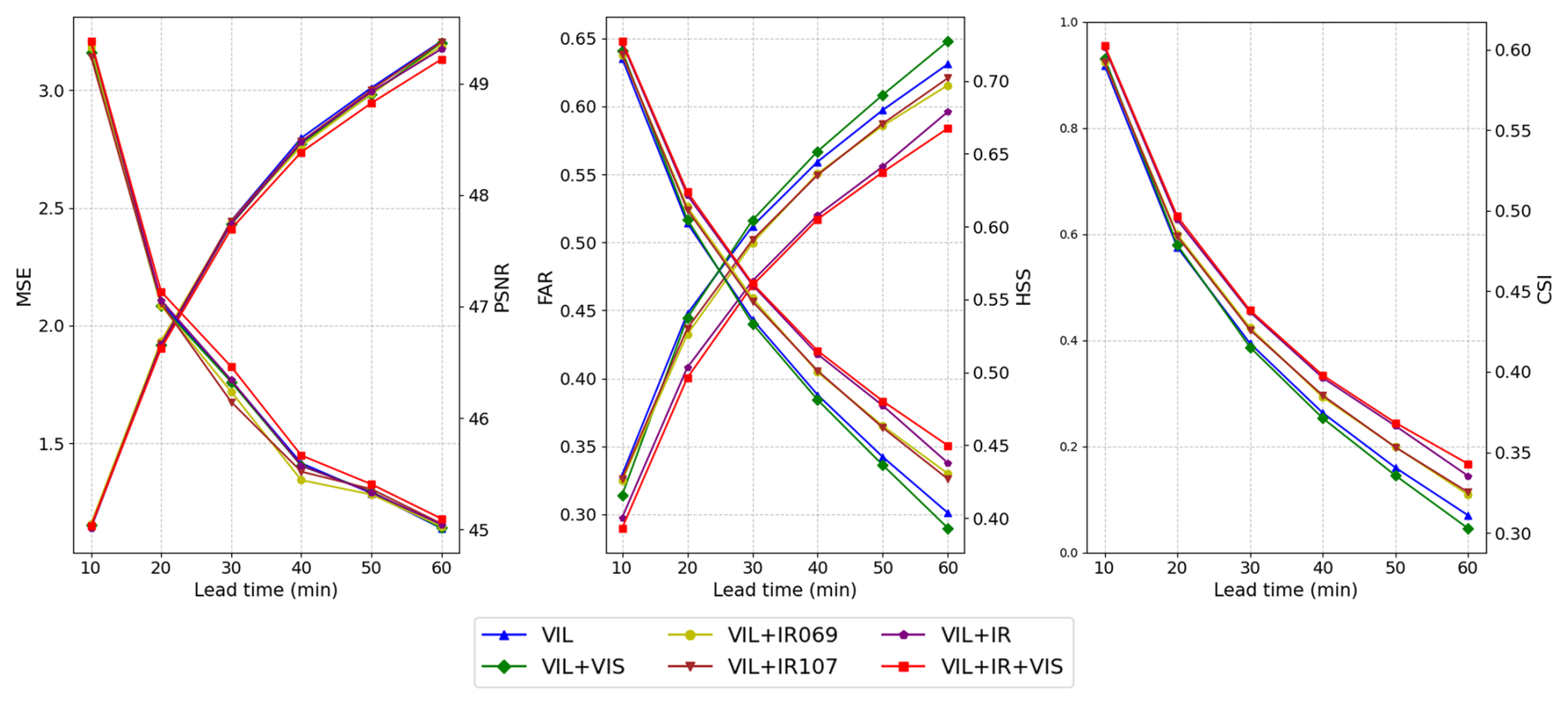
Figure 10 The index timeliness chart of all methods with a lead time of 60 min, MSE and FAR are all gradually increasing with time. PSNR, CSI and HSS are all gradually decreasing with time increasing.

5.4 Ablation Study

5.4.1 The Impact of Additional Meteorological Factors

The SEVIR dataset contains additional meteorological variables. In the aforementioned experiments, we utilized four different meteorological variables as inputs to the model, such as satellite mid-level water vapor, satellite infrared longwave window, satellite visible light, and radar vertical liquid water content. To assess the impact of incorporating additional dimensions of meteorological variables on the STI training framework, we systematically eliminated each type and quantity of the input meteorological variables. The experimental results are presented in Fig. 10. According to the delay theorem, increasing the spatial dimensionality of input data enables models to learn more spatial interaction features, thereby enhancing their capacity to establish nonlinear mapping relationships for future precipitation temporal information. The figure demonstrates that as meteorological variables diminish progressively, the STI-DEDN model exhibits a declining trend across all performance metrics with this degradation being most pronounced in the FAR indicator. This pattern suggests that employing more meteorological variables enhances the model's ability to remap spatial information onto future temporal patterns of precipitation variables effectively. Furthermore, the inclusion of additional variables enables better capture of intricate interactions and dependencies within atmospheric precipitation processes, thereby improving prediction accuracy.

5.4.2 The Results of Removing The STI Framework

To assess the optimization role of the STI framework in precipitation forecasting enhancement, we performed ablation studies through both framework exclusion (remove dual architecture and use only one-way training process) and its integration with other high-performing prediction models. While contemporary deep learning approaches have achieved commendable forecasting outcomes, climate change makes historical meteorological input data not reflect current atmospheric conditions accurately. Consequently, existing precipitation forecasting methods dependent on short-term temporal data frequently demonstrate inadequate performance in predicting extreme precipitation events. Integrating STI equations into precipitation forecasting methodologies enables the transformation of multidimensional spatial data into future temporal projections, thereby mitigating limitations that stem from short-term datasets. Ultimately, this approach enhances the performance of short-term precipitation forecasts. The experimental results are summarized in Table 9.

Table 9 Comparative experimental results after different methods ablated the STI frame, the best results are shown in bold.

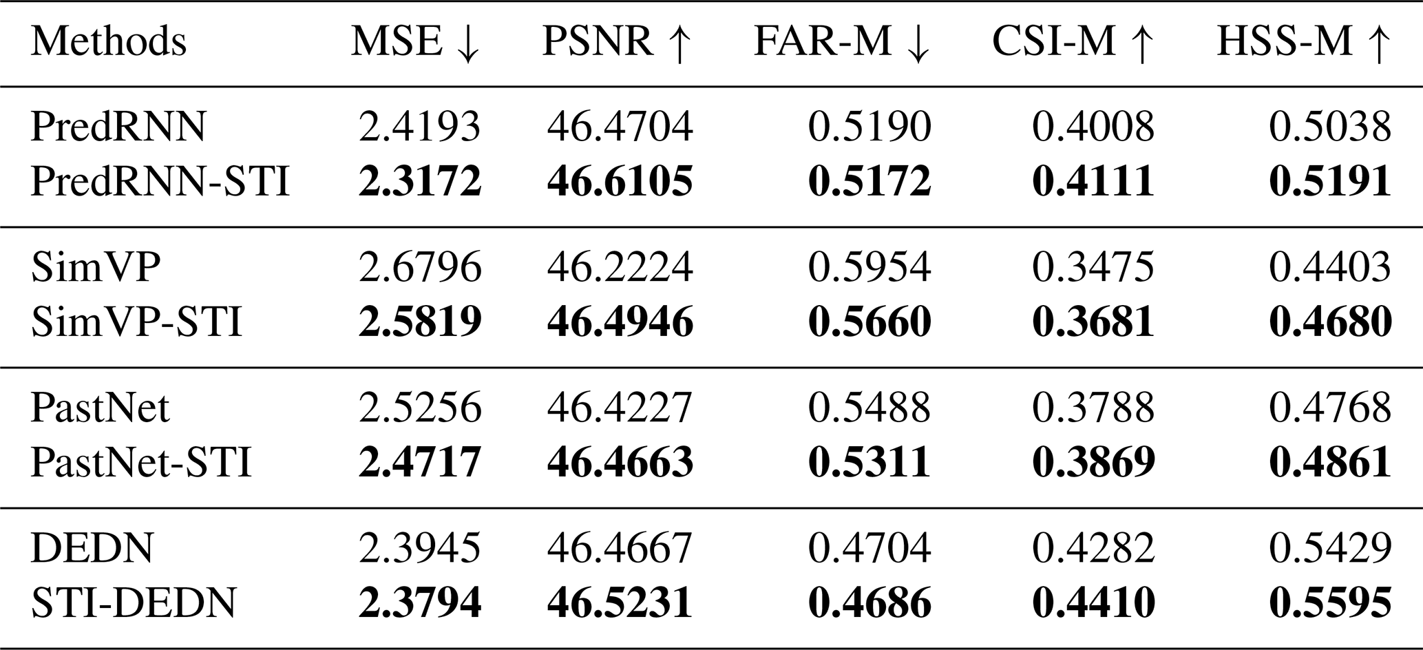
The experimental results demonstrate that it yields significant improvements across all quantitative metrics for each evaluated method incorporated STI. Notably, the ConvLSTM method exhibited enhancements of 13.05 % in MSE and 9.20 % in CSI.

All results highlight the efficacy and adaptability of the STI framework for spatiotemporal dynamic modeling. Models incorporated in the STI have higher performance on prediction accuracy and robustness, thereby yielding more precise precipitation forecasting outcomes.

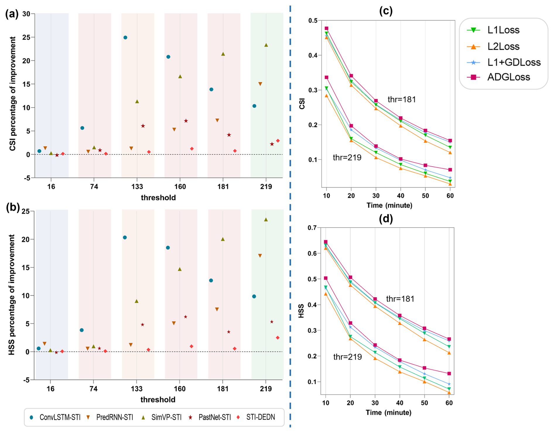
Figure 11 Panels (a) and (b) show the performance improvement of other methods after fusing the STI dual training framework at different thresholds compared with the original method. 0 value is equivalent to the original method without STI. Panels (c)–(d) show ablation experiments of different loss functions at thresholds 181 and 219.

Figure 11a, b show HSS and CSI improvements at all thresholds to assess how the STI architecture enhances precipitation events across intensity levels. The results indicate that the integration of the STI training framework yields positive enhancements in both CSI and HSS for all methods evaluated. Notably, The improvements are most significant for moderate-to-high-intensity precipitation events. It demonstrates the efficacy of the STI dual training structure in mitigating short-term data limitations while improving the models' overall predictive performance.

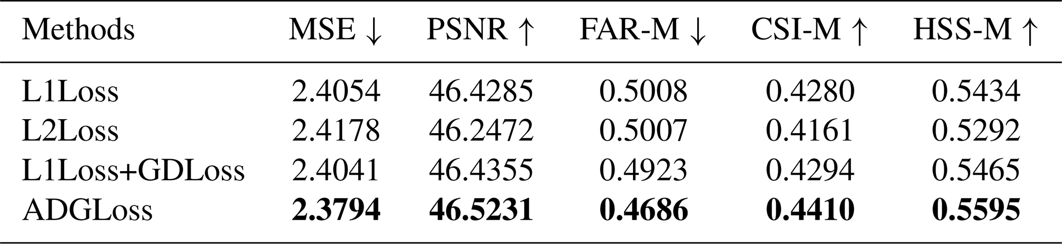
Table 10 Results of ablation experiments for loss of function, the best results are shown in bold.

5.4.3 The Results of Removing The ADGLoss Loss Function

Conventional regression-based loss functions fail to adequately capture abrupt extreme rainfall events frequently which is caused by climate change, resulting in systematic underestimation of moderate-to-severe precipitation events. To address this issue, we propose the ADGLoss, which effectively optimizes the model's sensitivity to the occurrence of extreme precipitation events, thereby enhancing predictive accuracy. We employed L1 Loss, L2 Loss, and a version of ADGLoss without weighting as loss functions to train the model and assess its performance. The experimental results are presented in Table 10 and Fig. 11c, d.

The ablation results of the loss function quantitatively demonstrate that the proposed loss function achieves the optimal performance. In particular, it improves the False Alarm Rate (FAR) by 6.41 % compared to the suboptimal loss function. Furthermore, the performance curves for different time horizons reveal that ADGLoss maintains a leading position under high-threshold precipitation conditions. Notably, as the forecast time increases, the decline in ADGLoss performance is minimal, indicating that our loss function effectively mitigates the exacerbation of errors associated with increasing forecast time, thereby enhancing the accuracy of moderate to severe precipitation predictions. Furthermore, to verify the impact of the loss function on the underestimation of precipitation, we randomly selected a set of events from the test set and plotted qualitative visualization analysis diagrams, as shown in Fig. 12. It can be seen from the figure that after applying GDLoss, the clarity of the boundary parts of the precipitation field at all lead times is significantly improved, and the image blurring effect is effectively suppressed. This is because GDLoss imposes explicit constraints on the gradient information of precipitation structures, which can better preserve the detailed texture features of precipitation areas. Further observation reveals that with the introduction of adaptive weight parameters, the intensity of heavy precipitation areas is closer to the real field, which successfully alleviates the problem of heavy precipitation underestimation.

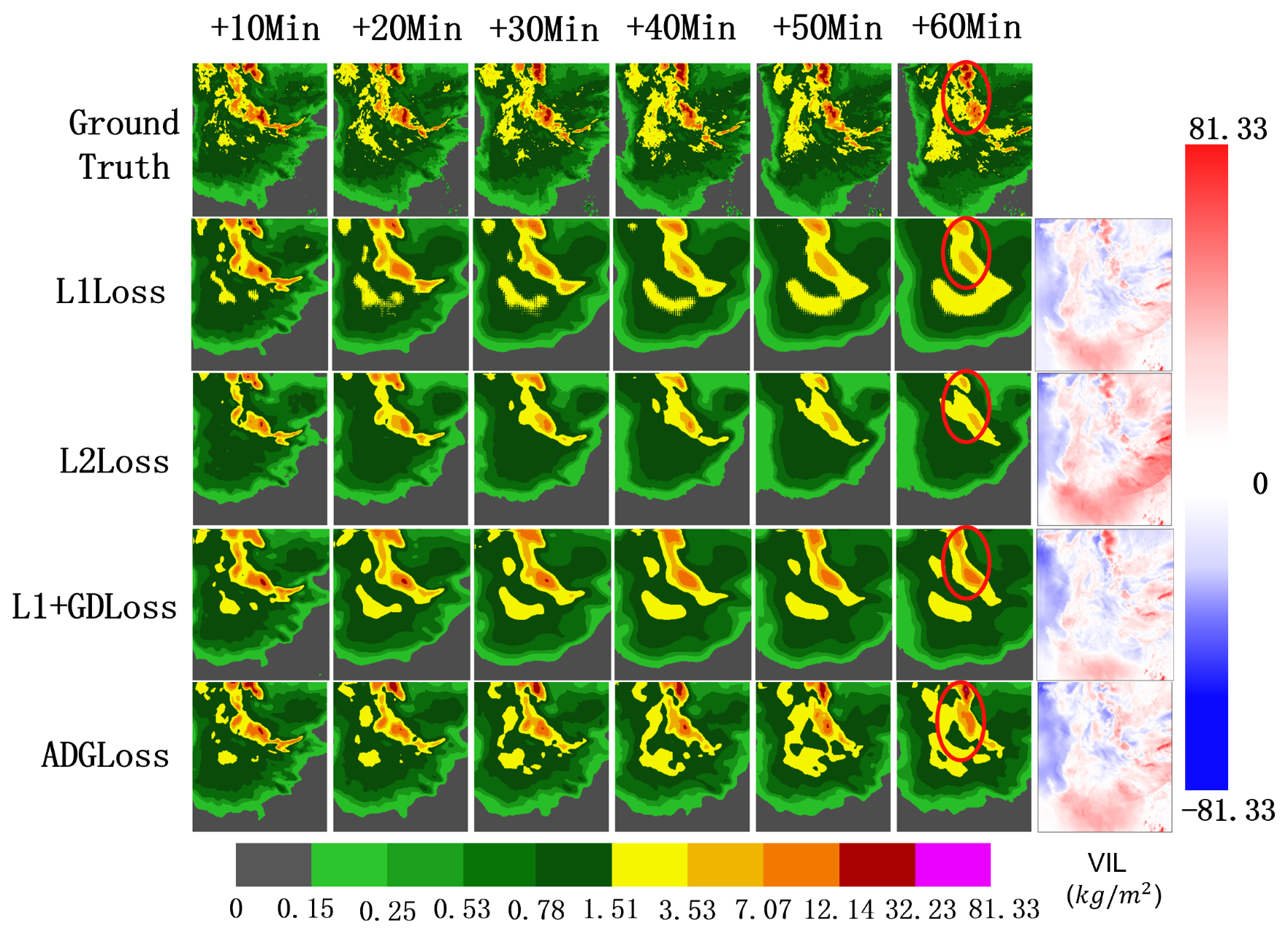
Figure 12 Visualization of precipitation maps and error heatmaps for all methods in the loss ablation experiments.

6 Conclusions

Current precipitation forecasting faces two key challenges: the limited accuracy of medium-to-heavy precipitation predictions based on short-term data, and a general tendency to underestimate precipitation intensity. To address these issues, we propose the STI-DEDN training framework, which combines the transformational principles of STI equations with the spatiotemporal modeling strengths of ConvLSTM to enable multi-step precipitation prediction from multidimensional meteorological inputs. The core innovation lies in leveraging dual learning to approximate the nonlinear STI mappings, enhancing the expressiveness and efficiency compared to traditional linear solutions. Additionally, we introduce ADGLoss, which adaptively reweights loss based on prediction difficulty, improving model focus on extreme precipitation regions and mitigating the issues of error amplification and precipitation underestimation caused by the extension of prediction time. Extensive experiments on multimodal datasets demonstrate that STI-DEDN outperforms existing deep learning methods in one-hour precipitation forecasting. Furthermore, integrating STI into other models yields up to an 8.60 % improvement in HSS, confirming the effectiveness of the STI formulation. It is worth considering that our work uses a SEVIR dataset that cannot be correlated at the temporal, seasonal, regional, or storm system levels. The randomized division of this dataset may overestimate the generalization ability of the model, which provides a direction for our future research. Future work will explore incorporating richer meteorological variables and addressing data imbalance issues and long-term forecasting error accumulation through improved augmentation strategies and effective attention mechanisms. In addition, future work will also break through the limitations of the SEVIR dataset to carry out more real-world precipitation forecasts, and conduct experimental analysis under relevant constraints such as different time, season, and region to improve the generalization ability of the model.