The TIPMIP Earth system model experiment protocol: phase 1

We describe a new Earth system model (ESM) experiment protocol, as part of the international Tipping Points Modelling Intercomparison Project (TIPMIP) project. We propose this as a protocol for the Coupled Model Intercomparison Project 7 (CMIP7). The protocol requires ESMs to run in CO₂-emission mode, with atmospheric CO₂ a predicted variable. Forcing for the protocol consists solely of a constant emission of CO₂, based on each model's transient climate response to cumulative emissions of carbon dioxide (TCRE) value, to give a common global mean surface warming rate of 2 °C per century. This positive emission (ramp-up) experiment is started from the pre-industrial state of a given model. When the ramp-up run first exceeds a specified level of global warming (2 and 4 °C) relative to the model's pre-industrial global mean surface air temperature (GMSAT), CO₂ emissions are set to zero and the positive emission run is branched into a zero-emission run. The zero-emission runs continue for 300 years. 50 years into each zero-emission run, CO₂ emissions are set to the negative of the positive emission rate and the model run until GMSAT cools below the original pre-industrial value. Additionally, when the negative emission run started from the global warming level (GWL)=4 °C first drops below GWL=2 °C, a zero-emission run is branched off this, completing the set of experiments. Using this protocol, we are able to control the rate of global warming, and potentially also the rate of cooling, across participating models. TIPMIP experiments will support a range of analyses, including; an assessment of abrupt/rapid Earth system change under net zero CO₂ emissions at a range of global warming levels, the long-term Earth system response to net zero CO₂ emissions at these warming levels, the response to net negative CO₂ emissions and the efficacy of negative emissions to drive cooling, and the reversibility of Earth system change under a pathway of positive (warming), zero, and negative (cooling) CO₂ emissions.

1 Introduction

We describe the Tier 1 experiment protocol to be followed by coupled Earth system models (ESMs) contributing to the Tipping Points Modelling Intercomparison Project (TIPMIP) (Winkelmann et al., 2025). This protocol (termed TIPMIP ESM Tier 1) has been designed as a simple (idealized) way to intercompare ESM simulations forced sequentially by positive, zero, and negative carbon dioxide (CO₂) emissions. The protocol controls the rate of increase in global mean surface air temperature (GMSAT, referred to here as the rate of global warming) across ESMs during the positive emission phase, with a rate of ∼2 °C per century chosen to approximate the observed global warming rate over the past ∼50 years. The protocol ensures ESMs branch from positive to zero CO₂ emissions at the same GWL, after the same rate and duration of warming. Finally, models branch into net negative CO₂ emission pathways (CO₂ removed from the atmosphere, at a rate mirroring the positive emission rate used in each model) after a common time period under zero emissions.

There is increasing interest in global warming overshoot scenarios (i.e. temporary exceedance of a global warming target that is returned to at some later date, Schleussner et al., 2024; Reisinger et al., 2025) and in the long-term response of the Earth system to net zero CO₂ emissions at temperatures warmer than today (Allen et al., 2022; Fankhauser et al., 2022). Key outstanding questions include, the likelihood, timing, and magnitude of overshoot, the consequences arising from such an overshoot, the feasibility of cooling the planet back from a peak warming to a (stabilized) target level, the potential for hysteresis once a stabilized climate is achieved, and the long-term response of the Earth system to net-zero emissions at temperatures warmer than today.

Our protocol lends itself to addressing a number of these questions. Areas of particular interest include (i) the risks and consequences of triggering Earth system tipping points (Winkelmann et al., 2025), (ii) residual warming and global to regional Earth system change under long-term zero emissions at different GWLs i.e. the zero emission commitment (ZEC) (Jones et al., 2019), (iii) the overall efficacy of negative CO₂ emissions in driving global cooling, including regional patterns of this cooling, and (iv) the reversibility of any induced changes following a net negative CO₂ emission pathway.

The protocol assumes ESMs are run in CO₂-emission mode, meaning atmospheric CO₂ concentrations are a predicted model variable, dependent on the prescribed emissions and the response of each model's carbon cycle. Such an approach allows a more complete simulation and analysis of the coupled climate–carbon cycle response to positive, zero, and negative CO₂ emissions. An effort to develop an analogous experiment protocol for models run in (prescribed) CO₂-concentration mode is underway and will be reported in a subsequent paper. This ESM protocol will be complemented by related experiments in TIPMIP (Winkelmann et al., 2025) using standalone, domain-specific models such as land-vegetation models, ocean models, and ice sheet models forced by output from these ESM experiments.

TIPMIP ESM experiments began as part of CMIP6plus (an extension to CMIP6 after the formal project had closed). This paper describes the experiment protocol in detail as preparation for participation in CMIP7 (Dunne et al., 2025). 38 MIPs have so far registered to take part in CMIP7, with the full list available at WCRP: https://wcrp-cmip.org/mips/#registered-mips (last access: 9 February 2026). TIPMIP has some commonality, and potential for collaboration with a number of CMIP7 MIPs, including C4MIP, CDRMIP, AERA-MIP (Silvy et al., 2024), as well as ScenarioMIP (van Vuuren et al., 2026) and the flat10MIP experiments (Sanderson et al., 2025) that are part of the CMIP7 Assessment Fast Track (Dunne et al., 2025). We discuss areas of potential collaboration with these MIPs in Sect. 3.4. An important feature of TIPMIP is that global warming in the positive emission (ramp-up) phase is common across models, Models branch into net zero emission runs after a common duration and rate of global warming, at the same GWL. Models run with zero emissions for a common time period (50 years) before switching to a negative emission (ramp-down) phase, with all models using the (negative) mirror image of the (ramp-up) positive emissions. Models are required to run in CO₂-emission mode, allowing us to assess the co-evolution of atmospheric CO₂ and climate under net zero emissions at common starting GWLs. The protocol also allows an assessment of ZEC at different GWLs, over 300 (potentially 500) years. In addition, the protocol enables analysis of the efficacy of negative emissions to drive cooling, from different GWLs, when both the natural carbon cycle and climate are able to freely respond to the imposed changes in atmospheric CO₂ (the prescribed negative emissions). The protocol is easily extendable to; (i) sample net zero emission responses at different GWLs (e.g. 1.5 or 3 °C) started from existing ramp-up and ramp-down runs, (ii) sample the change in the rate of cooling and climate reversibility as a function of the prescribed negative emissions (e.g. $\mathrm{1}/\mathrm{2}$ or $\mathrm{1}/\mathrm{4}$ of the original rate), and (iii) the implications of a delay in the onset of negative emissions (global cooling) from a given net-zero (GWL) run. For example, starting negative emissions after 200 years of net zero emissions rather than 50 years. Many of the simulations needed to make these additional runs will have been completed in the Tier 1 set of experiments and the technical implementation of these extensions is trivial.

2 Terminology and definitions

Tipping points occur in the Earth system where positive feedback loops are strong enough to induce self-sustained and often rapidly increasing change beyond a critical threshold, which drives the system from one preferred (equilibrium) state to another, with potential – negative consequences for human societies and natural ecosystems (Lenton et al., 2008, 2023; van Nes et al., 2016; Armstrong McKay et al., 2022). The tipping point is the critical level of forcing (for example, CO₂ emissions, or deforested area) that initiates tipping dynamics, (e.g. maintained melt leading to collapse of (parts of) an ice sheet). Tipping can also be induced when the rate of change of forcing exceeds a critical value, or stochastic variability leads to the initiation of nonlinear positive feedbacks (“rate-induced” and “noise-induced” tipping, Chapman et al., 2024). The nonlinear nature of the tipping process has two important consequences: (i) the ensuing change is often abrupt with respect to the normal forcing of the system and/or rapid with respect to the typical timescales of the system, and (ii) the change is often associated with a strong hysteresis, i.e. is practically irreversible, at least on societally relevant timescales. For example, if, after a warming overshoot, much colder temperatures are required to regrow an ice sheet to its pre-tip size than the temperatures that led to its collapse (Garbe et al., 2020). Abruptness and irreversibility are often consequences of the strong positive feedback loops but not necessarily a defining criterion for a tipping point. More details on the definitions and associated key terminology related to tipping points can be found in the recent TIPMIP overview paper (Winkelmann et al., 2025, e.g. see their Box 1).

The TIPMIP ESM Tier 1 experiments focus on four primary “tipping elements” of the biophysical Earth system that have been shown to potentially exhibit tipping (or abrupt change) behaviour: (i) the Atlantic Meridional Overturning Circulation (AMOC), (ii) Greenland and Antarctic ice sheets, (iii) boreal and tropical forests, and (iv) (ground) permafrost. In addition, the TIPMIP experiments enable analysis of a wide range of other system responses, including, but not limited to, the North Atlantic subpolar gyre (SPG), sea ice systems, and modes of climate variability.

Previous theoretical (Stommel, 1961; Rooth, 1982) and modelling work (Swingedouw et al., 2007; Jackson et al., 2015; Liu et al., 2020) has demonstrated the capacity for, and consequences of, a collapse of the AMOC. Using paleo-observations and modern sea surface temperature observations, Caesar et al. (2018, 2021) suggest the AMOC may have already entered a weakening phase, although significant uncertainty remains regarding the robustness and strength of such a weakening signal (e.g. Chen and Tung, 2018; Fraser and Cunningham, 2021; Kilbourne et al., 2022). Model projections also show a large spread in the future AMOC evolution, with the global warming level at which tipping may occur not well-constrained (Ben Yami et al., 2024). Studies also indicate susceptibility of the Greenland (Noël et al., 2021; Gregory et al., 2020; Robinson, et al., 2012), East Antarctic, and West Antarctic ice sheets and sub-glacial basins (Feldmann and Levermann, 2015; Garbe et al., 2020; Van Breedam et al., 2020) to irreversible decline beyond certain thresholds. Again, the thresholds for such behaviour are not well-constrained and thus formulating robust policy advice is difficult (Armstrong-McKay et al., 2022). Polar amplification has led to significant Arctic warming, as evidenced by rapid sea-ice loss (Taylor et al., 2022). Model projections indicate the first ice-free day in the Arctic could occur before 2030 (Heuzé and Jahn, 2024), with the potential to trigger tipping of multi-stressors affecting the marine ecosystem (Myksvoll et al., 2023; Heinze et al., 2021).

Dynamic global vegetation models (DGVMs), employed in coupled ESMs, have long demonstrated the capacity for rapid Amazon dieback (Cox et al., 2000; Good et al., 2011; Parry et al., 2022). A mounting body of work suggests the possibility of both climate and deforestation induced tipping, not only in the Amazon (Boers et al., 2017; Drijfhout et al., 2015; Lovejoy and Nobre, 2018), but also the boreal forest (Booth et al., 2012; Gerten et al., 2013; Koven, 2013). Similar studies show the potential susceptibility of permafrost systems to rapid, potentially irreversible change (Lenton, 2012), but stress that continued loss of permafrost with incremental warming means there is likely no “safe” level of warming for permafrost (Nitzbon et al., 2024). Furthermore, the trajectory followed to warming stabilization, characterized by the intensity and duration of warming overshoot, may lead to multiple steady states of high northern latitude soils, including carbon concentrations and fluxes, with potentially long-lasting effects after stabilization (de Vrese and Brovkin, 2021).

Considerable uncertainties remain around the critical forcing thresholds necessary to induce tipping, in particular the magnitude and duration of change, (Ritchie et al., 2025; Stocker and Schmittner, 1997). While there are increasing efforts to study tipping dynamics in offline, domain-specific models (Naughten et al., 2023; Bochow and Boers, 2023; Garbe et al., 2020), relatively few attempts have been made using coupled Earth system models, where dynamic feedbacks between Earth system components are explicitly modelled. While offline models are computationally less expensive, and in some cases offer more comprehensive treatment of individual tipping element dynamics, coupled ESMs are more likely to capture interactions between the phenomena at risk of tipping, as well as processes driving (or stabilizing) such a tipping risk. Coupled ESMs are also more suitable for investigating interactions between tipping elements (i.e. the risk of tipping cascades) and the broader climatic, environmental, and socio-economic consequences of tipping events (Wunderling et al., 2022; Franzke et al., 2022; Klose et al., 2020). This protocol is the first coordinated effort to investigate tipping point risks using coupled ESMs and responds to the concerns around tipping points risks in the future and the need for more research in this critical area (Ritchie et al., 2026; Lenton et al., 2025)

While the TIPMIP ESM Tier 1 protocol is focussed on coupled Earth system models, output from our simulations will be used across TIPMIP to force domain-specific models (e.g. ice-, ocean-, and land-only models) to study in detail domain-specific processes controlling the potential for tipping in these systems.

3 Experimental design: Tier 1 experiments

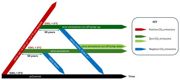
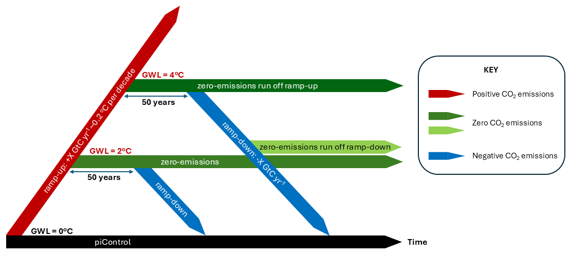
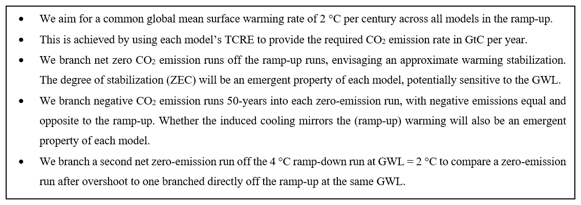
In this section we describe in detail the experiment protocol to be followed by contributing models. Figure 1 presents a schematic of the protocol and Box 1 summarizes the key assumptions underpinning the protocol. All experiments are to be run in CO₂-emission mode. The foundation of the protocol is a pre-industrial control simulation (esm_piControl). Once the esm_piControl is deemed sufficiently stable, a positive CO₂-emission (ramp-up) simulation is branched from the esm_piControl, with initial conditions taken from that run on 1 January of the selected year (defined as year A). The ramp-up run is forced by a positive global mean CO₂ emission rate of X Gt C yr⁻¹ (equivalently X Pg C yr⁻¹) where X is diagnosed from the model's TCRE (transient climate response to cumulative emissions of carbon dioxide, Allen et al., 2009; Matthews et al., 2009) to give a global mean surface air temperature (GMSAT) warming rate of 2 °C per century. The most accurate method to calculate TCRE is using the new flat10 experiment protocol (constant CO₂ emission of 10 Pg C yr⁻¹), as documented in Sanderson et al. (2025). If only a transient 1 % CO₂ run (1pctCO2) is available then we recommend the method of Arora et al. (2020, their Eq. 21 reproduced below) for calculating TCRE.

$$\begin{array}{}\text{(1)}& \text{TCRE}={\displaystyle \frac{\mathrm{\Delta }{T}_{\mathrm{2}\times {\mathrm{CO}}_{\mathrm{2}}}}{{\stackrel{\mathrm{‾}}{E}}_{\mathrm{2}\times {\mathrm{CO}}_{\mathrm{2}}}}}\end{array}$$

Where $\mathrm{\Delta }{T}_{\mathrm{2}\times {\mathrm{CO}}_{\mathrm{2}}}$ is the Transient Climate Response (TCR), defined (for a given model) as the change in GMSAT relative to its pre-industrial value at the time atmospheric CO₂ concentrations in a 1pctCO2 run (Eyring et al., 2016) have doubled, occurring after 70 years. ${\stackrel{\mathrm{‾}}{E}}_{\mathrm{2}\times {\mathrm{CO}}_{\mathrm{2}}}$ is the cumulative carbon emissions at the time of CO₂ doubling in the same experiment. TCRE is expressed in units of °C per exagramme (1000 Pg) of carbon. As an example, assuming a model TCRE of 2.5 °C per 1000 Pg C, to realize a global warming rate of 2 °C per century implies a carbon emission rate of $(\mathrm{2.0}/\mathrm{2.5})\times \mathrm{1000}\mathrm{Pg}\mathrm{C}=\mathrm{800}$ Pg C per century or 8 Pg C yr⁻¹. Because using the TCR approach may lead to slight deviations from the intended warming rate, this approach can be slightly modified (i.e. TCRE values slightly adjusted) to ensure a 2 °C per century warming rate. We recommend groups aim for a global warming rate of $+\mathrm{2}\pm \mathrm{0.1}$ °C for the first century of the positive emission run. As the ramp-up run reaches higher warming levels there is a greater risk warming rates in some models deviate from the target rate. With respect to the geographical pattern of the positive CO₂ emissions, we suggest emitting with a pattern that mirrors that used for the CMIP6 historical CO₂ emissions (for example the pattern of emissions for the final year of the CMIP6 historical period, 2014), scaled to give the required TCRE-based emission rate.

Figure 1 Schematic of the TIPMIP ESM phase 1, tier 1 experiment protocol.

Apart from the introduction of positive CO₂ emissions, everything else in the ramp-up is unchanged from the esm_piControl. The esm_piControl should be extended for as long as required to parallel the longest ramp-up → zero-emission → ramp-down → zero-emission run employed in the protocol. Details of these, and the recommended length of the esm_piControl, are provided below in Table 1.

Table 1 List of runs forming the TIPMIP ESM phase 1, tier 1 experiment protocol.

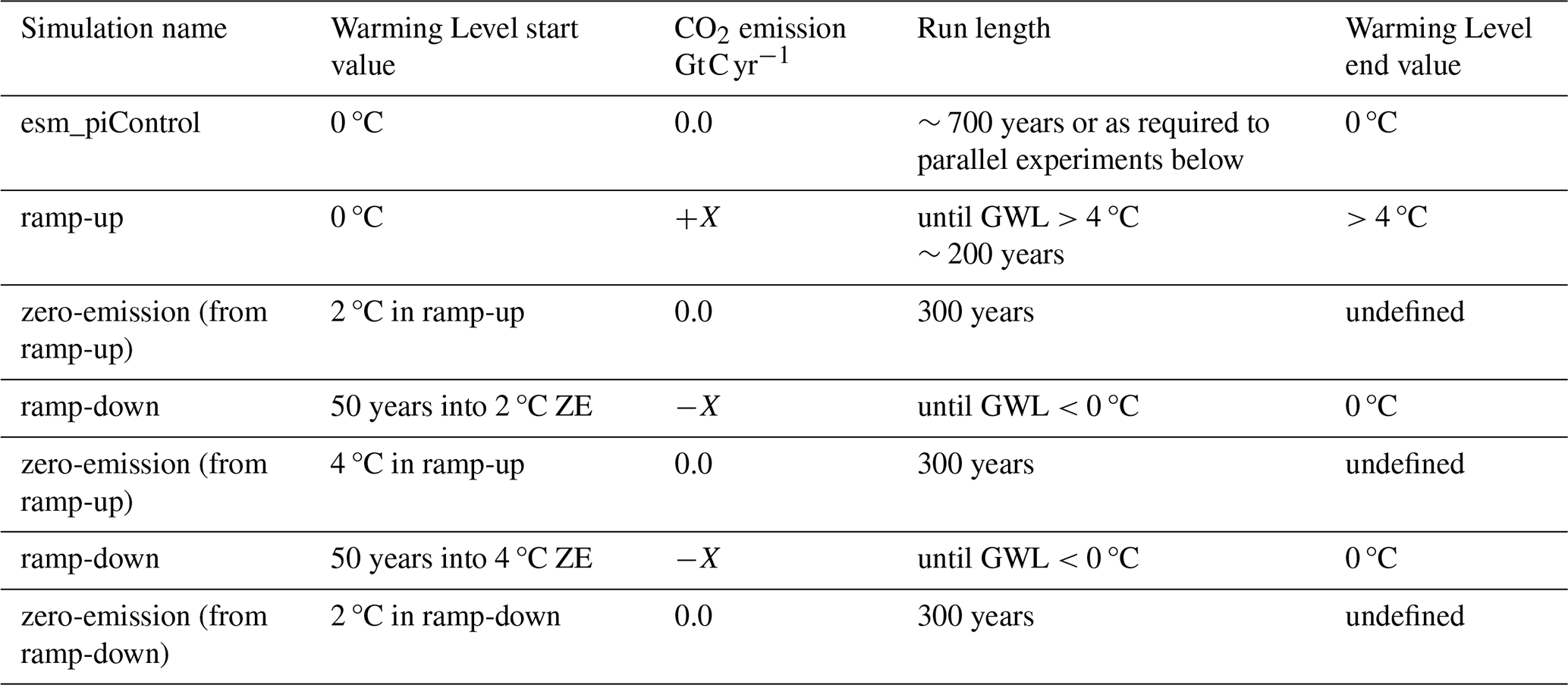
When GMSAT in the ramp-up run first exceeds a value 2 °C warmer than the esm_piControl (i.e. GWL=2 °C), CO₂ emissions are set to zero and a zero-emission (ZE) run is branched off the ramp-up. The start date of the ZE run is defined by comparing a 31-year (centred) mean GMSAT, for each year of the ramp-up, to the 31-year mean GMSAT centred on the year in the esm_piControl from which the ramp-up started. The ZE run start date is defined as 1 January of the year directly after the first year GWL=2 °C is diagnosed. The ZE simulation is run with CO₂ emissions set to zero for a minimum of 300 years. 50 years into the ZE run (i.e. 1 January of year 51), a ramp-down run is branched, with CO₂ emissions set to minus the value of the ramp-up run (i.e. −X Gt C yr⁻¹). The spatial pattern of negative emissions we leave to each modelling group to decide on, with two extreme options being (i) a mirror image of the pattern of positive emissions in the ramp-up or (ii) a spatially uniform pattern. This ramp-down run is continued until its 31-year mean GMSAT is less than the original 31-year mean centred on the year in the esm_piControl from which the original ramp-up started. At this point the ramp-down run can be stopped. Figure 1 illustrates this esm_piControl → ramp-up → zero-emission → ramp-down procedure.

The original ramp-up run is continued until its GMSAT first exceeds 4 °C warmer than the esm_piControl, calculated in the same way as for GWL=2 °C. At this year a second ZE run is branched off the ramp-up and run for 300 years. 50 years into this ZE run a X Gt C yr⁻¹ negative emission ramp-down is started and run until its GMSAT value is less than the original esm_piControl value. Finally, when the 31-year running mean GMSAT in the ramp-down, started from GWL=4 °C, first becomes colder than 2 °C above the original esm_piControl GMSAT, a second ZE run at GWL=2 °C is branched off the ramp-down. This procedure is shown visually in Fig. 1. Box 1 summarizes the main assumptions underpinning the experiment protocol and Table 1 the various simulation steps.

Box 1 Key assumptions and aims of the TIPMIP ESM protocol.

3.1 Caveats to the experiment protocol

An important positive aspect of the TIPMIP protocol is its simplicity, with only CO₂ emissions (positive, zero, and negative) needing to be prescribed. Using emission rates derived from each model's TCRE, we aim to control the GMSAT warming rate to be common across models during the ramp-up, and ensure models switch to zero-emissions at the same global warming level, relative to their pre-industrial temperatures, after the same rate and duration of global warming. These assumptions rest on an assumed linearity of TCRE across warming levels (and increasing cumulative CO₂ emissions) in the ramp-up. Put another way, we expect a unit emission of CO₂ (X Gt C) to cause the same unit increase in global mean surface air temperature (Y °C), whether the unit emission happens early in a ramp-up run (when accumulated CO₂ emissions and induced warming are relatively small) or later in the same run (when accumulated CO₂ emissions are larger and induced warming is also larger). This assumption of linearity appears accurate at lower warming levels (modest accumulated CO₂ emissions) but becomes less accurate at higher warming levels (greater accumulated CO₂ emissions), resulting in a slight deviation in some models in the rate of warming away from the target 2 °C per century at higher GWLs (Krasting et al., 2014). The degree to which this deviation complicates our analysis will be one important outcome of the first round of simulations and will inform further development of the protocol. While any global warming rate could, in principle, be realized, we chose 2 °C per century as this is the approximate rate of observed warming over the past ∼50 years.

We do not explicitly control the evolution of GMSAT in the zero-emission runs. Our a priori expectation is that changes in GMSAT during these phases (the Zero Emissions Commitment (ZEC), Jones et al., 2019) will be close to zero (MacDougall et al., 2020). That said, each model's ZEC response is an emergent property of that model – which may depend on global warming level and even on the length of the zero-emission run. While we force the ramp-down runs to have a negative, mirror image emission of the ramp-up, this does not guarantee each model will cool at −2 °C per century. The realized cooling rate in each model will depend on the amount of excess heat sequestered during the ramp-up and zero-emission phases, as well as how the carbon cycle, atmospheric CO₂ concentrations, and climate, respond in each model during the negative emission phase. We might expect a near mirror image ramp-down global cooling, but this too will be an emergent property of each model, likely related to its ZEC (Koven et al., 2023). It is important to reiterate our experiment protocol aims to control the evolution of GMSAT across models, acknowledging this may only be approximated in the zero and negative emission phases. In doing this, the cumulative CO₂ emissions in each model will differ significantly. For example, while models all branch into zero-emission runs at the same GWL after the same duration of warming, the cumulative emitted CO₂ and the atmospheric CO₂ concentration at this branch point will differ across models. This is a direct result of controlling for GMSAT at the expense of cumulative CO₂ emissions and needs to be considered in analysis of the resulting ensemble.

We choose a negative emission rate in the ramp-down that is a mirror image of the ramp-up to investigate the degree of symmetry in global warming and cooling under opposite and equivalent positive and negative emissions. This level of negative emissions (ranging from −8 to −18 Gt C yr⁻¹ depending on each model's TCRE) is clearly far greater than anything technically feasible today and probably also in the future (Gidden et al., 2025). We therefore recommend in the potential extensions to the phase 1 experiments (Sect. 3.2) that groups repeat the ramp-down phase using smaller negative emission rates (e.g. 50 %, 25 %, 12.5 % of their original rate).

While the simplicity of our protocol is a strong positive, it is also its main weakness. This is notably because we ignore other important anthropogenic forcings. In particular, emissions of aerosol and aerosol precursors. The protocol does include natural aerosols (as simulated in each individual model esm_piControl), including any response of natural aerosols to warming/cooling along the simulation pathway. Anthropogenic aerosols have provided an important (time varying, spatially heterogeneous) negative radiative forcing during the historical period (1850 to near present-day), balancing a significant fraction of the historical warming due to greenhouse gas (GHG) emissions (Gillett et al., 2021; Smith and Forster, 2021). In recent decades anthropogenic aerosol emissions have decreased, impacting the Earths top of atmosphere (TOA) Energy Imbalance (Quaas et al., 2022; Yuan et al., 2026; Loeb et al., 2025), potentially contributing to an acceleration of global warming (Foster and Rahmstorf, 2026) Aerosol emissions also vary significantly across different future emission scenarios, such as the CMIP6 Shared Socioeconomic Pathways (SSPs) (Gidden et al., 2019). Due to their short atmospheric lifetime and strong interaction with low-level clouds (Williams and Igel, 2021; Fons et al., 2023) anthropogenic aerosol forcing has a specific geographical structure (Wilcox et al., 2023). Over the historical past, aerosol induced cooling is far greater in the Northern Hemisphere (NH) than in the Southern Hemisphere (SH), while GHG forcing is more homogeneous. As a result, the total historical anthropogenic radiative forcing at the top of atmosphere (TOA) has a distinct NH to SH gradient. This gradient, as well as the detailed spatial structure of aerosol forcing, will not be captured in our protocol and may have important consequences for simulated AMOC changes (Menary et al., 2020).

A second important omission is human land-use. Human land use has provided a negative forcing of the Earth system over the historical period. For example, in the HadGEM3-GC3.1 CMIP6 historical run, human land-use forcing was −0.11 W m⁻², ∼6 % of the total historical anthropogenic forcing in that model (Andrews et al., 2019). At regional scales, particularly with respect to tropical forests and their resilience, human land use (i.e. deforestation) plays a critical role (Flores et al., 2024), potentially of similar importance to global climate change (da Cruz et al., 2021, Boulton et al., 2022). For potential tipping of forest ecosystems (particularly the Amazon) our experiment protocol therefore neglects an important driver. Introduction of human land-use and anthropogenic aerosol are high priorities for a tier 2 set of experiments, but require careful testing before they can be included, as our aim will be to retain as much commonality as possible in warming pathways across models.

The protocol does not consider non-CO₂ anthropogenic GHG emissions, such as methane (CH₄), ozone (O₃), nitrous oxide (N₂O) or chloroflurocarbons (CFCs and HCFCs). While these are important forcers, for example when combined giving an historical radiative forcing ∼75 % of that due to anthropogenic CO₂ emissions (Chap. 7, IPCC, 2023a), their lifetime, horizontal distribution, and impact primarily on the longwave part of Earth's radiation budget, suggest to a first order their forcing can be mimicked by an equivalent CO₂ emission. Omission of anthropogenic CFCs and HCFCs also means there will be no stratospheric ozone depletion (Solomon, 2019) in our experiments.

Because our protocol is forced solely by CO₂ emissions, with no aerosol or other well-mixed greenhouse gas (WGHG) emissions, it is likely that when the idealized runs reach GWL=2 and 4 °C (the start of the zero-emission runs) they will have experienced a larger cumulative emission of CO₂ than equivalent multi-gas and land-use scenarios at the same GWL. This is primarily because the positive radiative forcing arising from non-CO₂ WGHGs (e.g. methane, ozone, nitrous oxide etc) in the multi-gas scenarios is being achieved (in a warming sense) by CO₂ emissions in our idealized runs. This is partially offset by not including aerosol (negative radiative forcing). As a result, at common GWLs, models will have different atmospheric CO₂ concentrations and will have absorbed different amounts of emitted carbon into the ocean and terrestrial biosphere, impacting responses such as plant photosynthesis or ocean acidification. These caveats should be considered when analysing ecosystem responses.

The Tier 1 protocol requests only one member per model. This is to maximise the number of models contributing. In some cases, tipping events are expected to be rare occurrences. Hence, a large ensemble would help in sampling such events, including potential stochastic forcing of tipping (Romanou et al., 2023), while also helping identify when, and under what conditions, a tipping event is more likely to occur. This can be partially addressed by the multi-model aspect of the protocol, with 11 ESMs already running these experiments. Nevertheless, we recognize the need for more ensemble members. For instance, a bifurcation in the AMOC has been shown to exist in one ESM and could therefore have implications for the timing and reversibility of AMOC-related tipping (Romanou et al., 2023). We therefore encourage groups to consider running additional ensemble members (started from different time points in their esm_piControl) in the potential extensions to Tier 1. Similarly, the Tier 1 protocol asks for the zero-emission runs to be a minimum of 300 years in length. This is sufficient for investigating many Earth system responses, but for some of the slower Earth system components (e.g. ice sheets or the deep ocean) longer runs are required. We therefore encourage groups to extend their zero-emission runs to 500 years or longer, in the potential extensions to the Tier 1 protocol.

3.2 Potential extensions to the Tier 1 protocol: Tier 2 experiments

There are a number of highly desirable and technically straightforward extensions to the Tier 1 protocol, that we encourage modelling groups to consider running. These include:

• 1.

  Extending the three zero-emission runs shown in Fig. 1 to 500 years each (or as long as possible).

• 2.

  When the two ramp-down runs first pass GWL=0 °C (i.e. pre-industrial GMSAT), branch zero-emission (ZE) runs at GWL=0 °C and run these for 500 years (or longer).

• 3.

  Extend the original esm_piControl so it is sufficiently long to act as a reference for the zero-emission runs proposed under points 1 and 2.

• 4.

  In addition to zero-emission runs at GWL=2 and 4 °C, also perform zero-emission runs branched off the ramp-up and ramp-down runs at GWL=1.5, 3, and potentially 1.2 °C, approximating present-day global warming.

• 5.

  Repeat the negative emission runs sampling negative rates equal to 50, 25, and 12.5 % of the original −X Gt C yr⁻¹.

• 6.

  In addition to the negative emission runs starting 50 years into each zero-emission run, start identical negative emission runs later in the same zero-emission runs (after 200 years is recommended).

• 7.

  Increase the ensemble size e.g start new ramp-up → zero-emission → ramp-down legs of the protocol, as additional ensemble members branched from the esm_piControl. We suggest a minimum of 30 years separation in the esm_piControl between starting new ramp-up runs.

3.3 A reduced set of Tier 1 experiments: Tier1_reduced

To maximize the number of models contributing to TIPMIP, we also propose a reduced set of Tier 1 experiments. While we encourage groups to run the full set of experiments whenever possible, groups will be able to participate in Tier 1 by realising the reduced set of runs:

• An esm_piControl for 300 years.

• One ramp-up run at X Gt C yr⁻¹ to GWL=2 °C.

• One zero-emission (ZE) run at GWL=2 °C for 200 years.

• One ramp-down run (started 50 years into the ZE run at GWL=2 °C), run back to GWL<pre-industrial.

3.4 Links to other CMIP7 model intercomparison projects (MIPs)

The TIPMIP ramp-up and zero-emission simulations have similarities with the constant emission, zero-, and negative- emission simulations planned in CMIP7 flat10MIP (Sanderson et al., 2025). A key difference between the two sets of experiments is that the TIPMIP protocol aims to enforce approximate commonality across models in the temporal evolution of GMSAT; i.e. similar warming rates and duration of warming in the positive emission runs before zero-emission runs are branched at common GWLs. The zero and negative emission runs are not guaranteed to exhibit common temperature evolution across each model, these being an emergent property of each model. The protocol accepts the amount of CO₂ emitted into each model will necessarily be different to realize this. In flat10MIP, commonality in CO₂ emissions is enforced across models, while inter-model variability in the evolution of GMSAT is accepted. While there are similarities between the two sets of experiments, joint analysis of model responses in common-GMSAT versus common-CO₂ emission space will help understand differences seen between the two protocols when run by the same model. The flat10 set of experiments allow TCRE to be diagnosed for each ESM under a common emission rate of +10 Gt C yr⁻¹, which can be used to inform the positive emission rates in TIPMIP. TIPMIP simulations are more extensive and naturally follow on from flat10. They are designed to explore in more detail model responses, following close-to-uniform warming rates and sampling a number of common global warming levels at which net zero CO₂ emission runs are started. The state-dependence of ZEC and the response to negative emissions is a particularly useful and unique analysis opportunity offered by the TIPMIP simulations

Earth system change and regional patterns of change seen in the TIPMIP experiments can also be compared with results from ScenarioMIP (O'Neill et al., 2016; van Vuuren et al., 2026) and CMIP7 DECK (diagnostic, evaluation and characterization of klima) experiments (e.g. 1pctCO2 and abrupt 4×CO₂ runs, Dunne et al., 2025) at similar transient global warming levels. This will provide information on the impact of staying long-term at, or close to, a given GWL (in the TIPMIP zero-emission runs) compared to transiently passing through it. Attention will need to be paid to the fact the TIPMIP simulations are forced solely by variable CO₂ emissions. ScenarioMIP forcing is a multi-gas mix, including time varying aerosol emissions and human land-use. The latter, while more realistic, is more difficult to achieve commonality of GMSAT behaviour across models, which is a primary aim of the TIPMIP protocol.

A recent multi-model initiative, AERA-MIP (Silvy et al., 2024), provides 1.5 and 2.0 °C stabilization simulations that account for all anthropogenic drivers. This approach utilizes the adaptive emission reduction approach (AERA, Terhaar et al., 2022) to produce temperature stabilization simulations for two GWLs, following realistic historical forcing trajectories.

TIPMIP simulations can be compared with AERA-MIP results to explore, for example, the impact of non-CO₂ radiative forcing on the spatial patterns of climate change in the AERA-MIP runs stabilized at GWL=2 °C and the TIPMIP net zero-emission runs initialized at GWL=2 °C. This analysis will need to pay careful attention to the different experiment set ups in the two runs, particularly the inclusion of non-CO₂ forcers in AERA-MIP. A difference between the two protocols is the commonality of model warming rates in the TIPMIP ramp-up runs, as well as the commonality of GWL at which net-zero CO₂ emission runs start. We intend to compare tipping point behaviour in common model realizations of the two protocols at common GWLs.

In CMIP6, the Carbon Dioxide Removal Model Intercomparison Project (CDRMIP, Keller et al., 2018) explored the potential for, and impacts of, CDR deployment. In CMIP7, CDRMIP will address questions concerning the response of the Earth system to atmospheric CO₂ removal (negative CO₂ emissions), the efficacy of different CDR approaches, such as afforestation/reforestation and ocean alkalinization, and begin to assess active CDR as simulated in a number of ESMs, contrasting these with equivalent representations in Integrated Assessment Models (IAMs).

We have dubbed the TIPMIP Tier 1 protocol “see what happens” experiments. By this we mean the runs do not include any external interventions or forcings to ensure a tipping event occurs. There is a widespread feeling that ESMs may be designed (explicitly or unconsciously) to be overly stable with respect to tipping events (Rahmstorf, 2024; Valdes, 2011). This may result in only a small number of tipping events occurring in our Tier 1 ensemble. A natural extension to the TIPMIP protocol, in particular using the zero-emission runs started at GWL=2 and 4 °C, is to deliberately induce a tipping event in these simulations. This has the advantage of knowing, in advance, the climate state at which the tip occurs and automatically having a non-tipping counterfactual run sampling the same climate state as the tipping run. Tips can be induced by prescribing external forcing terms or by making targeted modifications to key model parameterizations to increase the sensitivity of a given system to climate forcing. Such forced tip “make it happen” experiments will be developed in collaboration with the domain-specific activities in TIPMIP, as well as TIPMIP-WHATIF (Winkelmann et al., 2025) to ensure widespread utility of the resulting experiments across projects.

3.5 Diagnostics for all phase 1 experiments

The data request for TIPMIP starts from the data request for the esm-historical experiment in CMIP6. In a first step the number of requested variables was reduced to only include variables that 3 sample ESMs were able to produce, assuming these provide a reasonable subset of CMIP6 models. The list was further reduced by excluding most variables at sub-daily frequencies. TIPMIP experiments cover several centuries, and the amount of data would become impractical if sub-daily data, especially on multiple levels, were saved. The reduced list was then passed to TIPMIP domain experts for inspection, which resulted in some additional variables that were considered important for analysing domain specific tipping points. TIPMIP ESM output will be used as forcing for offline models in TIPMIP. We also anchored our diagnostic list with the Inter-Sectoral Impact Model Intercomparison Project (ISIMIP) (Frieler et al., 2024) to ensure data can be used to force sectorial impact models. All diagnostics follow CMIP6plus CMOR (climate model output rewriter) protocols. CMIP7 protocols will be used once they are fully established.

3.6 File naming conventions

TIPMIP comprises a number of zero-emission (ZE) simulations at specific GWLs, as well as positive CO₂-emission (ramp-up) and negative CO₂-emission (ramp-down) experiments that link one warming level with another. A ZE experiment branching directly off a ramp-up experiment will therefore be different from another ZE experiment, at the same GWL, branching off a ramp-down experiment itself started from a higher GWL value. To distinguish between these two experiments, we propose a naming convention that allows us to construct experiment names by using short blocks describing each experiment phase and then adding these blocks together to form unique experiment_ids for each possible experiment. The building blocks and example experiment file names are listed below in Tables 2 and 3.

Table 2 Building blocks of the naming schemes for creating experiment_id's. These form the basis of the output filenaming convention for TIPMIP under CMIP6plus.

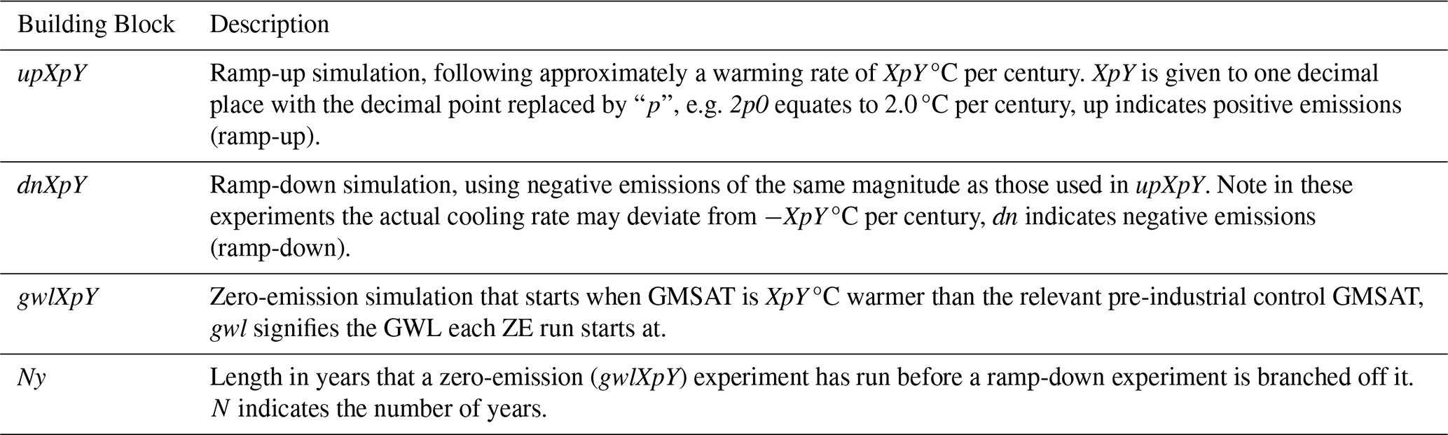
Table 3 experiment_id and experiment attribute for the TIPMIP ESM phase-1 experiments. The prefix “esm-” follows CMIP6 standards and indicates that these are CO₂ emission driven experiments. The experiment names form the basis for identifying different runs under the TIPMIP protocol for a given model.

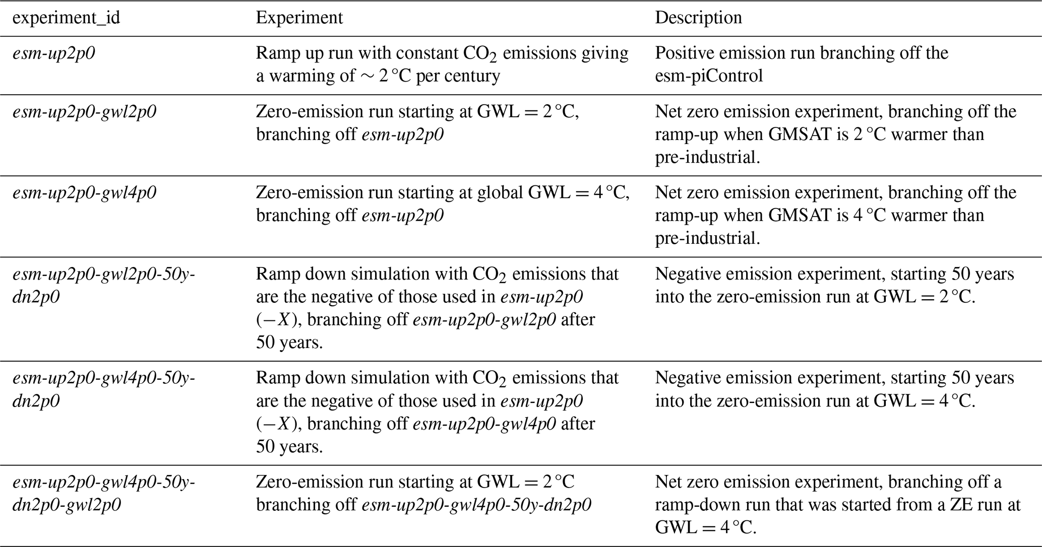
The building blocks are combined to identify the full history of a given experiment, forming part of the output filename for a given model. By using these building blocks, it is possible to distinguish ZE experiments at different GWLs that have started directly off a ramp-up run, from those that have started after a ramp-up, ZE run at a higher GWL, and ramp-down back to the GWL of the ZE run in question, or distinguish between experiments with different length ZE runs before a ramp-down run is started. Table 3 lists the experiment_id and experiment metadata for the Tier 1 experiments.

4 Science questions to be addressed

4.1 Tipping points and abrupt change

Tipping of Earth system elements is often considered a low-likelihood, high-risk event that may result in severe consequences for ecosystems, biodiversity, and society. In recent years there has been increasing evidence that several parts of the Earth system are already undergoing rapid, potentially irreversible change (Lenton et al., 2008, 2019), which may lead to crossing of tipping points. Components at risk of tipping include the West Antarctic and Greenland ice sheets, Amazon and some boreal forests, savanna and dryland ecosystems, coral reefs, the Atlantic Meridional Overturning Circulation (AMOC), the North Atlantic Subpolar Gyre (SPG), and ground permafrost. (e.g. Levermann and Winkelmann, 2016; Sgubin et al., 2017; Staal et al., 2020; Swingedouw et al., 2020, 2021; Chap. 9, IPCC, 2023a; Armstrong McKay et al., 2022). Recent studies estimate that widespread, at least partly irreversible, mass loss from the West Antarctic ice sheet may be triggered when global warming levels range from 1–3 °C above pre-industrial (Golledge et al., 2017; Garbe et al., 2020; Reese et al., 2023). For the Greenland ice sheet, a critical threshold is estimated in the range 0.8–3 °C of global warming, with a best estimate of about 1.5 °C (van Breedam et al., 2020; Noël et al., 2021; Höning et al., 2023). The recent Global Tipping Points Reports (Lenton et al., 2023, 2025) conclude that some Earth system tipping events are no longer low-likelihood, high-impact events, rather they are rapidly becoming high-likelihood, high-impact events.

Large uncertainty still exists with respect to tipping point risks. Many studies use a range of observational data including paleo-proxy records, in situ measurements, as well as atmosphere and ocean reanalyses. Satellite data, covering the past few decades, is also playing an increasing role (Swingedouw et al., 2020; Lenton et al., 2024), because of its global coverage at fine temporal and spatial resolution. In situ data is often spatially too coarse, and satellite data temporally too short, to reliably detect early warning signals of tipping events. ESMs offer global coverage at reasonable (but by no means sufficient) spatial resolution and can be integrated for multi-centuries. ESMs can therefore be used to investigate where, when, and how, tipping events are triggered (Romanou et al., 2023; van Westen et al., 2024a, b), as well as how different tipping systems interact. Studies to date have mostly been based on either a single model, and/or individual experiment design, with a focus on individual tipping element (e.g., the North Atlantic Hosing Model Intercomparison Project (NAHosMIP) and AMOC, Jackson et al., 2023).

A key aim of the TIPMIP ESM protocol is to investigate a range of tipping events using a common experiment protocol sampled by multiple ESMs. We aim to investigate the risk of tipping events under net zero emissions initiated at different levels of global warming, and if triggered, whether the ensuing changes are reversible (through global-scale cooling) on societally relevant timescales. Ritchie et al. (2021, 2025) stress both the peak global warming level (GWL), and the duration spent at a given GWL before cooling, are important determinants of the risk of triggering a tipping event. The TIPMIP Tier 1 protocol offers a (minimal) set of multi-model experiments to address such tipping risks (i) under net zero emissions started at two different GWLs, (ii) associated with the duration of net zero emissions, and (iii) the potential for reversibility as warming is reduced.

A number of studies have identified abrupt changes in ESMs (Drijfhout et al., 2015; Swingedouw et al., 2021), including stochastic collapse of the AMOC (Romanou et al., 2023), localized, rapid Amazon loss (Parry et al., 2022), and rapid, irreversible mass loss of the West Antarctic ice shelf (Naughten et al., 2023). In addition, van Westen et al. (2024a) show how a freshwater flux into the Atlantic in the CESM model can induce positive feedback driving a collapse of the AMOC. They further highlight such feedback is poorly represented in present-day models, due to large biases in simulated salinity fields. van Westen et al. (2024b) extend this work to derive a fingerprint for AMOC collapse (based on surface ocean buoyancy), which they apply to an ensemble of CMIP6 projections, finding a greater than 50 % likelihood the AMOC will pass a critical point for tipping during the 21st century following a middle-of-the-road emission scenario. With respect to permafrost, recent studies emphasize the need to incorporate frozen soil thaw dynamics and associated carbon release into models to accurately estimate available carbon budgets (Natali et al., 2021; Turetsky et al., 2020). CMIP6 ESMs are capable of simulating gradual permafrost thaw but lack the necessary resolution and process representation to capture the spatial heterogeneity of permafrost thaw dynamics. Quantifying the impact of missing processes is essential for advancing our ability to estimate future permafrost behaviour. Offline models representing high northern latitude terrestrial processes will be forced by TIPMIP ESM output to help refine estimates of annual permafrost thaw using the methodology of Burke et al. (2020), and improve predictions of potential rapid loss of permafrost volume.

For many of the phenomena at risk of tipping, ESMs exhibit biases in the representation of these phenomena (Li et al., 2021; McCarthy and Caesar, 2023) and in the climate drivers of the phenomena (Mecking et al., 2017; Robson et al., 2022; Jensen et al., 2024), including the representation of extreme events that might push a system beyond its resilience limits (Romanou et al., 2025). An important task is to assess the quality of the TIPMIP ESMs in simulating the phenomena of interest, the key climate controls of these phenomena, including those that control the risk (or not) of a phenomenon tipping. For this we will focus on established metrics and climate controls for each phenomenon, including statistical and physically based metrics (or fingerprints) that are considered robust indicators of a potential tip. In this respect, the development of robust observational constraint approaches (e.g. Portmann et al., 2025) is important, as is the need for a large multi-model ensemble.

Once a tipping event is identified, we will assess: (i) the mechanisms underpinning the event, comparing the key driving processes across the multi-model ensemble (MME); (ii) whether there are early warning signals of the tip and then search for the occurrence of similar indicators across the MME; (iii) the broader consequences of any tip for the rest of the Earth system, considering both remote impacts (Ritchie et al., 2020) and interactions between components of the Earth system (Klose et al., 2024). Systems at risk of tipping have the potential to interact (i.e. if one regional system tips, cascading teleconnections can influence the risk of a tip in another remote system Wunderling et al., 2024). An ESM dynamically couples different Earth system processes. The TIPMIP protocol allows us to investigate potential tipping point interactions across models, supporting quantification of any interactions and possible cascades.

4.2 Long-term change under zero emissions at different global warming levels

The Paris Agreement aims to limit global warming to below 2 °C (and pursue efforts to limit warming to 1.5 °C). GMSAT has already increased by almost 1.5 °C and cumulative GHG emissions continue to increase (Friedlingstein et al., 2025). It is therefore unclear when, and at what level, temperatures (and associated emissions) might be stabilized in the future. It is also unclear if, how, and how rapidly, global temperatures can be reduced, for example through net negative CO₂ emissions. It is possible global temperatures remain significantly above present-day values for a long period before any significant cooling occurs. Furthermore, Gillett et al. (2011), Cassidy et al. (2024), and Chamberlain et al. (2024) show strong regional changes in climate, particularly over the Southern Ocean, following net-zero emissions even when global mean temperatures are approximately stable. Continued Southern Ocean warming, particularly at depth, is associated with a slowing of the overturning circulation at subpolar latitudes, decreasing the export of cold Antarctic Bottom Waters into the global ocean (Chamberlain et al., 2024). The amount of heat released from the Southern Ocean may also affect the dependence of ZEC on the level of (surface) warming at which zero emissions are realized. MacDougall et al. (2020) found in a limited number of ZECMIP models that higher levels of cumulative emissions may lead to greater ZEC values.

It is therefore urgent to understand how the Earth system will respond to net zero emissions at different GWLs (King et al., 2021, 2024; Chamberlain et al., 2024; Silvy et al., 2024). Such analysis requires long-term, zero-emission simulations at a range of GWLs. The TIPMIP protocol provides such a data set.

Slow processes, such as melting of ice sheets or deep ocean warming, will continue to evolve long after net-zero emissions are achieved. Paleo evidence suggests a committed global sea level rise of around two meters per degree of global warming on millennial time scales (Levermann et al., 2013; Pattyn et al., 2018). Continuous freshwater input to the ocean, from melting land ice, will also have long-term impacts on ocean circulation (Swingedouw et al., 2007; Hu et al., 2008). As long as the ocean is still adjusting, feedbacks onto other components of the Earth system, expressed through changes in marine heat and carbon fluxes (DeVries et al., 2017; Rugenstein et al., 2020), have the potential to impact patterns of regional change.

The potential for gradual warming under net-zero emissions may result in system thresholds being exceeded, with impacts on ecosystems and society, or even tipping of elements in these systems, such as abrupt shifts in vegetation (Wei et al., 2025), regime shift in marine primary productivity (Vasilakopoulos et al., 2017), biodiversity loss (Ureta et al., 2022) or permanent displacement of people (Defrance et al., 2017). Furthermore, gradual change in the mean climate can induce shifts in modes of regional climate variability (Horton et al., 2015; Tamarin-Brodsky et al., 2020; Kim and An, 2024), with consequences for extreme events (Fischer et al., 2021; Wehrli et al., 2022). The TIPMIP protocol offers the possibility to study both incremental climate change and associated regional changes in variability in long-term, zero-emission simulations.

While climate change is not yet one of the top drivers of biodiversity loss (Jaureguiberry et al., 2022), it is emerging as a significant threat (Soultan et al., 2022; Kubelka et al., 2022). Recurrent extreme temperature or precipitation events impact the ecology of different disease vectors (Liu-Helmersson et al., 2014) and put stress on agriculture and infrastructure (Sgubin et al., 2019). The TIPMIP ESM experiments will be used to drive impact models in ISIMIP (Frieler et al., 2024) to investigate such risks to ecology, biodiversity, and society.

Most studies to date looking at climate impacts at a given GWL have been based on transient projections, analysing periods where global warming falls in an interval around a given target level (Lennard et al., 2018; Tebaldi et al., 2021; Swaminathan et al., 2022). These studies suffer from the fact that the transient climate at a certain warming level differs from the climate after a longer period at the same level. In many regions, this leads to differences between the transient and the equilibrium climate at the same GWL (King et al., 2020, 2024; Lacroix et al., 2024). The TIPMIP zero-emission simulations offer the opportunity to assess the long-term response of the Earth system to net zero CO₂ emissions at different GWLs. Key questions to address include:

• What are the long-term regional changes under net-zero emissions and do these changes differ depending on the GWL at which net-zero emissions are realized?

• What impacts are avoided by achieving net-zero emissions at one GWL compared to a warmer GWL?

• What are the benefits of pursuing negative emissions (global cooling) from a given GWL versus net-zero emissions at the same GWL? I.e. what impacts are avoided through negative emissions relative to net-zero emissions?

• How different is the climate response to net-zero emissions at a given GWL depending on the path followed to reach that GWL (i.e. with or without a temporary warming overshoot and subsequent ramp-down cooling)?

• If thresholds for tipping key elements are exceeded, can irreversible tipping be avoided through deployment of negative emissions and global cooling?

To answer these questions robustly, an ensemble of simulations is required. Single model simulations can differ significantly from each other, examples include Arctic Sea ice (Notz et al., 2020) and AMOC (Weijer et al., 2020), and their subsequent evolution in future projections (e.g. Romanou et al., 2023). Regional climate change patterns are even more challenging as they strongly depend on large-scale circulation patterns and internal variability (Kjellström et al., 2018; Koenigk et al., 2020). Internal variability can be partially addressed by the long zero-emission simulations. However, as the mean state keeps evolving, late and early periods in these simulations may be different. In addition, ESMs simulate different regional and cascading changes across Earth system components at the same GWL (Evin et al., 2024). Dealing with these model-to-model differences calls for an ensemble of models running the same set of experiments. The Tier 1 protocol requests 300-year zero-emission simulations. This may not be sufficiently long to fully answer questions pertaining to the new equilibrated state at different GWLs. It is therefore important to link with activities looking at timescales exceeding a few hundred years (King et al., 2024; Rugenstein et al., 2020).

4.3 Reversibility

The IPCC Special Report on the Ocean and Cryosphere in a Changing Climate (SROCC) (IPCC, 2022a) defines reversibility as the ability of the Earth system to reverse anthropogenic-induced changes and return to a state equivalent to that prior to the external perturbation (e.g. a preindustrial condition), on a certain timescale. Irreversibility, in contrast, implies a suite of forcings and system responses that moves the system across some critical threshold, from one stable equilibrium to another (Lenton et al., 2008), with the original state unattainable under reasonable bounds of modified forcing or time periods. Irreversibility or hysteresis is often related to tipping events (van Nes et al., 2016; Armstrong McKay et al., 2022; Lenton et al., 2023), although irreversible change can also occur as a result of incremental warming or climate change.

Current literature suggests irreversible Earth system change may result either from nonlinear responses to an external forcing, or state-dependent responses to this forcing, or a combination of both ( Litzow and Hunsicker, 2016; Scheffer et al., 2015; Santana-Falcon et al., 2023; Heinze et al., 2023; Ritchie et al., 2023; Fröb et al., 2024). The question whether changes are reversible is therefore connected to the response of key processes to variable external forcing (Frölicher and Joos, 2010; Kug et al., 2022), where this forcing might be external to the Earth system (e.g. anthropogenic CO₂ emissions or solar variability) or internal to the Earth system but external to a specific phenomenon (e.g. changed ENSO variability and its impact on Amazon resilience). Details of the external forcing matter, for example, changes in either the magnitude or duration of forcing, such as the rate of warming or the magnitude and duration of warming overshoot, are thought to be important factors in driving a system towards irreversible change (Schwinger and Tjiputra, 2018; Jeltsch-Thömmes et al., 2020; Ritchie et al., 2023, 2025).

The TIPMIP experiments allow us to address questions around the potential reversibility of Earth system change. A first question concerns the reversibility of global warming realized in the positive emission (ramp-up) phase. One might expect equal and opposite negative emissions to induce global cooling of a similar rate to the (ramp-up) warming. This is not necessarily the case for the TIPMIP runs, as each model's response during the 50 years of zero emissions will differ, resulting in different GMSAT and atmospheric CO₂ values across models at the start of the negative emission run. The spread in these quantities at GWL=4 °C may also be greater than at GWL=2 °C. Hence, while the linearity of TCRE and the link between cumulative emissions and peak warming suggest TCRE and TCRR are symmetric, for the TIPMIP ensemble this needs to be established. While previous assessments (e.g. IPCC Special Report on Global Warming of 1.5 °C, IPCC, 2022b; IPCC 6th Assessment Report WGI, IPCC, 2023a) provide some insight into how changes differ between warming levels, the question of how reversible the changes are, particularly regional changes, remains uncertain.

Another important question relates to how changes in one location (or component) of the Earth system can cause changes elsewhere. Emerging literature (Armstrong McKay et al., 2022; Lenton et al., 2023; Wunderling et al., 2024) suggest some tipping elements, once triggered, may influence the stability of other parts of the Earth system. The suggestion is that an initial global-scale change can induce a major regional (abrupt) change that itself amplifies the global-scale signal or triggers independent regional abrupt changes elsewhere (Wunderling et al., 2022). Quantifying these risks requires an improved understanding of region-to-region interactions in the Earth system. Recent studies highlight how anthropogenic forcing has the potential to significantly alter prominent modes of climate variability, such as the Inter-Tropical Convergence Zone (Kug et al., 2022) or the El Nino Southern Oscillation (ENSO, Vaittinada Ayar et al., 2022; King et al., 2024; Cassidy et al., 2024), with the potential to induce further, potentially amplifying regional responses in remote Earth system domains.

A third question concerns long-term committed change under net zero emissions at different GWL, such as Greenland or Antarctic ice loss, or permafrost thaw, and its potential reversibility when negative emissions (and cooling) are initiated. Recent work (Schleussner et al., 2024) suggests reducing global temperatures can limit long-term climate risks compared with merely stabilizing warming (i.e. negative emissions compared to net-zero emissions). However, there are deep uncertainties in the long-term response of the Earth system, associated with the severity and duration of warming before cooling is realized, as well as how accurately models represent the long-term features of the coupled Earth system. Recent advances in Earth system models participating in TIPMIP will help address this question. For example, ESMs now include interactive treatment of phenomena such as continental ice sheets, permafrost, wildfires, and are increasingly running in emission mode for GHGs, allowing a more complete representation of interactions between physical climate change and the carbon cycle (Sanderson et al., 2025).

4.4 Earth system responses to net negative emissions

The magnitude of global warming scales approximately linearly with cumulative CO₂ emissions (IPCC, 2023b). This underpins the expectation that global mean temperatures should approximately stabilize under net-zero CO₂ emissions, and that reducing CO₂-induced warming requires net negative CO₂ emissions. The TIPMIP ESM simulations will also allow us to explore the efficacy and implications of reversing global temperature through net negative emissions.

The linearity of warming arises from the climate response to forcing – both the transient response and the rate of adjustment to constant forcing – as well as the radiative forcing from CO₂ emissions (Allen et al., 2022), the latter controlled by the airborne fraction of emitted CO₂. The resulting relationship – known as the transient climate response to cumulative carbon emissions (TCRE) – gives a monotonic and approximately path-independent peak-warming response to CO₂ emissions. While some studies have shown this relationship may break down for both very large cumulative emissions and strong negative emissions (e.g. Zickfeld and Herrington, 2015; Zickfield et al., 2021), these results are based on single model studies. It remains unclear how symmetrical TCRE is (i.e. the extent to which TCRE under net negative emissions, also referred to as TCRR (Chimuka and Zickfeld, 2026), is equal and opposite to TCRE). Koven et al. (2022) show that deviations from reversibility of TCRE are related to the legacy response to previous emissions and correlate with the ZEC for each model – models with a positive ZEC show an overshoot of temperature under negative emissions while models with a negative ZEC may undershoot – i.e. they may reverse more quickly than the negative emissions alone would imply. Models with a ZEC close to zero are much closer to reversible along the same TCRE gradient. Models with a higher ZEC, and importantly if ZEC becomes increasingly positive at higher warming levels, may exhibit reduced sensitivity to negative emissions – i.e. they may cool slower than they warmed in the ramp-up phase. Extending the CMIP7 flat10MIP experiments (Sanderson et al., 2025), TIPMIP samples multiple GWLs, allowing a systematic analysis of multi-GWL responses to positive, zero, and net negative, emissions.

Carbon dynamics under negative emissions are qualitatively understood, although models differ in the quantitative magnitude of their response. Over the last century, CO₂ emissions have caused a rapid rise in atmospheric CO₂ concentration and natural carbon sinks – both land and ocean – while removing some of this, have not kept up and so increase their sink rates in step with the emissions (Raupach et al., 2014). When CO₂ emissions stop increasing, atmospheric CO₂ declines and natural sinks weaken, eventually saturating, in particular the land biosphere (Silvy et al., 2024). Under negative CO₂ emissions, atmospheric CO₂ concentration strongly declines, and the natural sinks eventually reverse as both ocean and land ecosystems outgas excess CO₂ (Tokarska and Zickfeld, 2015; Jones et al., 2016; Koven et al., 2022). Thus, in the long term, the same processes which lead to natural sinks opposing positive emissions also lead to the natural carbon cycle opposing CO₂ removal, i.e. for every ton of CO₂ removed (e.g. by CDR), atmospheric CO₂ concentrations will decline by less than one ton. Uncertainty in the carbon cycle response to negative emissions is likely dominated by land ecosystems in the same way as it is for the response to rising emissions (Jones and Friedlingstein, 2020), although on longer timescales the land sink will saturate more quickly leaving a larger role for ocean uptake (Randerson et al., 2015). The TIPMIP ESM experiments will enable quantification of the various contributions to the total carbon cycle response to negative emissions simulated in the latest generation of ESMs.

5 Initial results

We present a small set of examples of the TIPMIP experiment protocol in action, realized by a number of contributing ESMs. Further analysis is planned once the majority of models have completed the protocol and converted their data into a common format.

In Fig. 2, for one model (GFDL_ESM2M, Dunne et al., 2013), we show the full protocol pathway of, plotting global mean atmospheric CO₂ mixing ratio (referred to as atm.CO₂ hereafter) and global mean surface air temperature (GMSAT). We present the complete pathway from one model primarily for illustrative purposes. More robust conclusions will be developed through subsequent analysis of the full ensemble. The positive emission (ramp-up) run branches from an esm_piControl that is temporally stable with respect to both atm.CO₂ and GMSAT, with atm.CO₂ rising throughout the ramp-up to a value of ∼850 ppm by the time GWL=4 °C. GMSAT closely follows a warming rate of 2 °C per century through the ramp-up. At GWL=2 °C the zero-emission run sees a slow reduction in atm.CO₂ as the ocean and land continue to take up excess CO₂ from the atmosphere. This decrease in atm.CO₂ will lead to a negative trend in radiative forcing, which on its own would be expected to cause a decrease in GMSAT (Williams et al., 2025). This is not the case, with a ZEC value slightly above zero being realized in this model at GWL=2 °C. This slight positive ZEC indicates there is a committed warming at the branch point from the positive emission run into the zero-emission run, represented by heat taken up during the ramp-up residing in the subsurface ocean (Williams et al., 2025). During the zero-emission run this sequestered heat has time to reach the surface, balancing the cooling tendency from the decrease in CO₂, with the combined result being a small surface warming (i.e. a positive ZEC). In the zero-emission run started at GWL=4 °C there is a clear tendency for this model to have a more positive ZEC than at 2 °C. The model also shows varying timescales in ZEC, with near-zero ZEC during the first hundred years of the 2 °C zero emissions simulations, followed by a period of more continuous warming (Frölicher and Paynter, 2015). The two negative emission runs branched from the zero-emission runs at GWL=2 and 4 °C both show near symmetrical global cooling compared to warming in the ramp-up. The degree to which these findings hold for the multi-model ensemble will be assessed in forthcoming studies. The zero-emission run, branched at GWL=2 °C off the ramp-down started from 4 °C, also suggests a modestly positive ZEC. It is noteworthy that atm.CO₂ at the point GWL reaches 2 °C in the ramp-down is lower than atm.CO₂ at GWL=2 °C in the ramp-up, suggesting that to return to a GWL value of 2 °C after overshoot requires atmospheric CO₂ to be lower than for the same value of GMSAT before overshoot (Held et al., 2010).

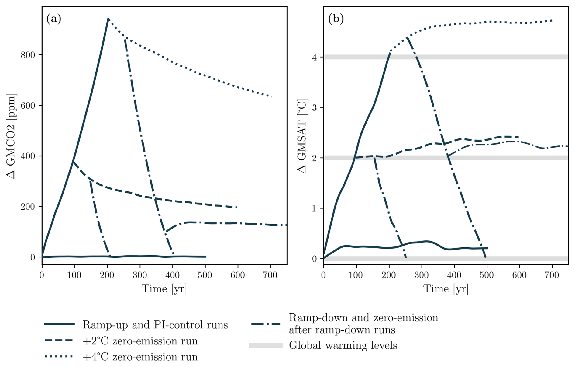
Figure 2 An example of the TIPMIP ESM protocol based on a single model (GFDL_ESM2M, Dunne et al., 2013) simulations. Panel (a) shows global mean atmospheric CO₂ concentration (atm.CO₂). Panel (b) shows global mean surface air temperature (GMSAT).

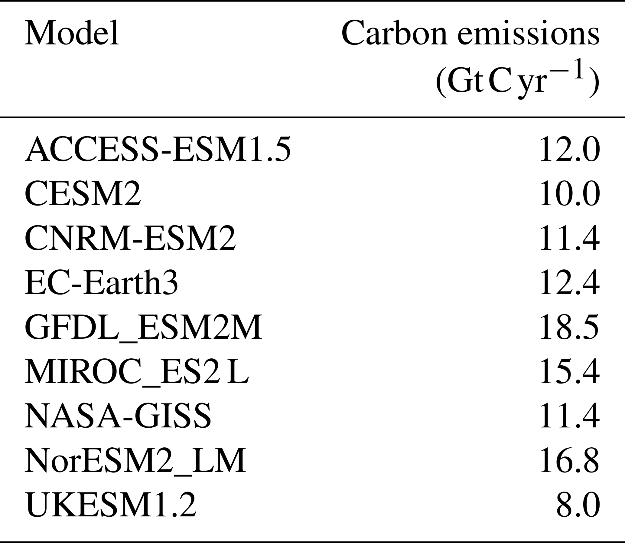
Figure 3 shows the same as Fig. 2, only for the positive emission (ramp-up) and zero-emission runs at 2 and 4 °C, this time for nine models that have so far made these runs. At the time of writing, not all models have completed the zero-emission runs, some have run 500 years of zero-emission while others have only run 300 years. We plot the full length of each model simulation. From the multi-model results, it is clear different CO₂ emission rates (and therefore different atmospheric CO₂ concentrations) are required to realize a near common 2 °C per century warming across models. Models closely follow the 2 °C per century warming from 0 °C (i.e. piControl) to 2 °C. Above GWL=2 °C there is more spread in warming rates, suggesting TCRE is not completely linear across all GWLs (and emitted CO₂) in all models. The combination of common warming rates driven by different atmospheric CO₂ increases means there is significant spread across models in atm.CO₂ at both GWL=2 and 4 °C, with this difference growing from 2–4 °C. Table 4 summarizes this by showing the annual carbon emissions for each model required to achieve a 2 °C per century global warming rate.

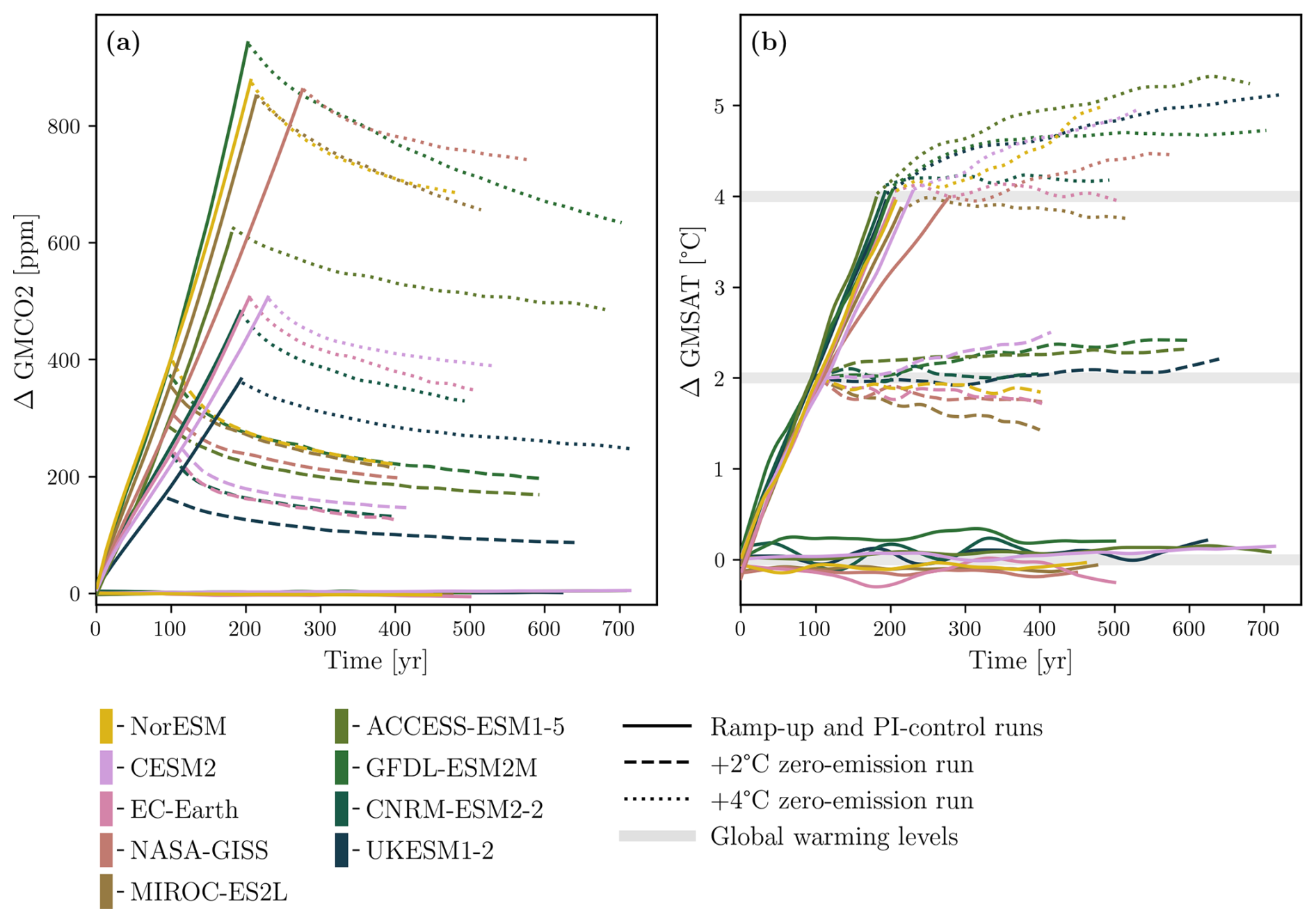
Figure 3 Global mean atmospheric CO₂ (atm.CO₂ in ppm, a) and GMSAT (°C, b) for the piControl (full line), ramp-up (full line) and zero-emission runs at GWL=2 °C (dashed lines) and 4 °C (dotted lines), as simulated by nine ESMs (listed in the figure legend).

Table 4 Annual carbon emissions in Gt C yr⁻¹ applied to each model to simulate a global mean surface air temperature increase of 2 °C per century in the positive emission phase of the protocol.

The ZEC response (trend in GMSAT) at 2 °C varies across models. A few models show negative ZEC and a few positive. While the ensemble mean ZEC is close to zero, it is important to highlight the uncertainty in ZEC at 100 years is $\sim \pm \mathrm{0.2}$ °C (or ±10 % of the total warming). The spread in ZEC increases at GWL=4 °C, with an increased tendency for positive ZEC across models, with a few models also suggesting ZEC becomes progressively more positive with time through the zero-emission run. The sensitivity of ZEC to the level of global warming at which zero emission are initiated, as well as to the duration of zero-emissions, is being investigated using the TIPMIP multi-model ensemble and will be reported in a forthcoming paper.

In Fig. 4 we plot the change in atm.CO₂ and GMSAT in the zero-emission run normalized to zero at the start value of each run. For atm.CO₂ we plot both the absolute change (in ppm) and the fractional change relative to the start value. Absolute atm.CO₂ decreases slightly more rapidly in the GWL=4 °C zero-emission run than in the one started at GWL=2 °C. When plotted as a fractional change there is less difference in the atm.CO₂ trend between these two GWLs. The absolute change in GMSAT, relative to the value at the start of the zero-emission run, is generally more positive at GWL=4 °C than at GWL=2 °C (i.e. only one model shows a very slight negative ZEC at GWL=4 °C while five models clearly show a significant positive ZEC at this GWL that is more positive than the value at GWL=2 °C).

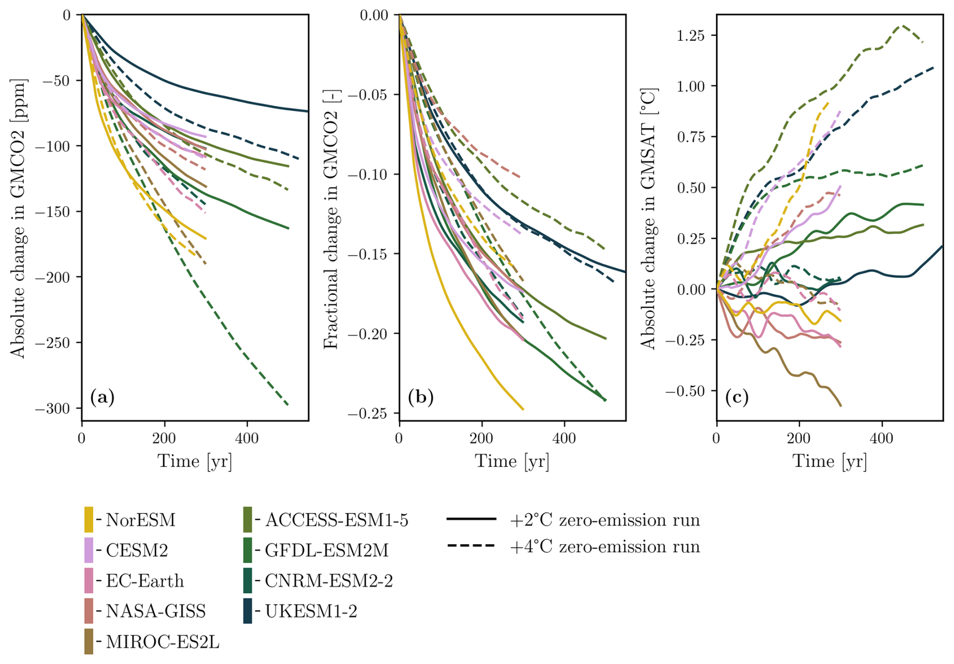
Figure 4 Change in global mean atmospheric CO₂ concentration and GMSAT for the two zero-emission runs expressed as anomalies relative to each value at the start of the respective zero-emission run. (a) Absolute change in atm.CO₂ in ppm, (b) fractional change in atm.CO₂, and (c) change in GMSAT in °C.

6 Summary and conclusions

We have introduced a new ESM experiment protocol, developed as part of the TIPMIP project (Winkelmann et al., 2025). The protocol assumes ESMs are run in CO₂-emission mode. The protocol requires a constant emission of CO₂, derived from each model's TCRE, to give a global mean warming rate of 2 °C per century. At specified levels of global warming (2 and 4 °C) relative to each model's pre-industrial global mean surface air temperature (GMSAT), CO₂ emissions are set to net zero and runs branched into zero-emission experiments that continue for 300 years (500 years if possible). 50 years into each zero-emission run, CO₂ emissions are set to the negative of the positive emission rate used in the ramp-up. These two negative CO₂-emission runs (started from zero emission runs at GWL=2 and 4 °C) are continued until GMSAT cools below the original pre-industrial GMSAT. When the negative emission run started from GWL=4 °C first drops below GWL=2 °C a zero-emission run is branched off this, completing the Tier 1 set of experiments.

While this experiment protocol is highly idealized (using only CO₂ emissions as a surrogate for all anthropogenic forcing), the resulting ensemble can be used to investigate (i) the risks, consequences, and drivers of abrupt/rapid Earth system change (tipping points) under net zero CO₂ emission, initiated at two global warming levels, (ii) the long-term response of the Earth system to net zero CO₂ emissions, (iii) the behaviour of the Earth system under prescribed net negative CO₂ emissions following a specified (magnitude and duration) of global warming overshoot, (iv) the efficacy of net negative CO₂ emissions in driving global cooling, and (v) the reversibility of Earth system change under a pathway of positive (warming), zero (near stabilization), and negative (cooling) CO₂ emissions. The primary advantage of the protocol is that we can control the rate of global warming and (potentially) cooling across models, using a TCRE-based CO₂ emission rate specific to each model. This enables a multi-model intercomparison of the above topics in a near common global warming/cooling space.

An initial analysis of the TIPMIP simulations shows that if CO₂ emissions drop to zero by GWL=2 °C, averaged across participating models, global warming will cease. This corresponds to achieving “Net Zero”. If, on the other hand, net-zero emissions are not realized until GWL=4 °C, our results suggest a continued, slow global warming for centuries thereafter, emphasizing the need (and benefits) of realizing Net Zero as rapidly as possible. The TIPMIP simulations will be extensively used to understand the mechanisms controlling the climate response after net zero emissions are reached, including the evolution of regional patterns of changes. In addition, the simulations will help in understanding the degree of climate reversibility at regional scales after a global warming overshoot, negative emissions and associated global cooling.

The protocol has now been run by 12 ESMs, and a common set of diagnostics is in the process of being published on the Earth System Grid Federation (ESGF), initially following the CMIP6plus protocol and subsequently CMIP7. We envisage further developing the Tier 1 experiment protocol in the coming years as part of CMIP7.