Integrating reservoirs and lakes in the CoSWAT global hydrological model

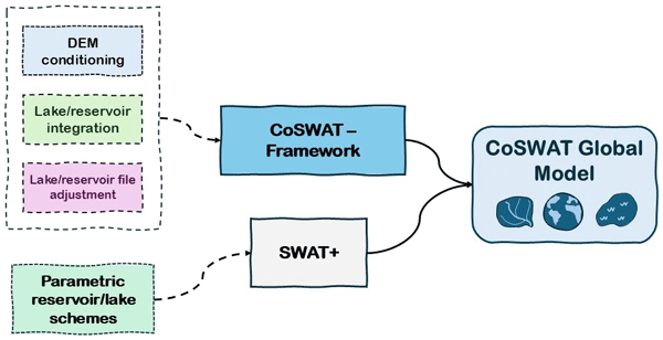
Global water models are essential tools for assessing water resource challenges in the context of climate change, land use changes, and human activities. The CoSWAT Global Water model is a global application of the Soil and Water Assessment Tool (SWAT+). It is a high-resolution tool designed to simulate water systems using a basin-oriented structure. The CoSWAT model currently lacks a realistic representation of reservoirs and lakes, limiting its ability to adequately represent basins where these water bodies play a significant hydrological role. The scarcity and limited accessibility of global reservoir operation or lake outflow data make it challenging to represent these water bodies with the current tools that SWAT+ supports, particularly at a global scale. In this study, we address this limitation by combining commonly used reservoir and lake modelling schemes from other global water models and the capabilities of SWAT+, and by implementing a topological approach to estimate irrigation water demands for reservoirs. We also introduce an improved workflow to integrate lakes and reservoirs into the river network, setting up the CoSWAT model at 0.01° resolution on selected regions worldwide, where validation of reservoir and lake storage, inflow, outflow, and the impact on streamflow performance was assessed. The results show that the model captures monthly storage dynamics with moderate performance. Overall, 34 % of evaluated reservoirs achieved a positive KGE, a performance comparable to other state-of-the-art global hydrological models, with CoSWAT surpassed by only two of five models in the comparison. Moreover, results demonstrate an improvement in performance in streamflow representation on 135 out of 192 (70 %) evaluated stations following the integration of lakes and reservoirs. Despite these improvements, persistent streamflow biases that consequently affect reservoir storage point to the need for hydrological calibration, which remains a priority for future developments. Overall, these methodological advancements represent a substantial improvement for the CoSWAT global model, enabling more robust and realistic assessments of inland water systems at the global scale.

1 Introduction

Rivers and lakes are essential for supporting ecosystems, providing access to water resources, preserving biodiversity, and regulating the water cycle. At the same time, reservoirs are crucial for water supply to different sectors, energy generation, and flood control. The combination of anthropogenic climate change, driven by alterations in the land use and land cover (LULC), human activities, and socio-economic shifts, has unequivocally affected climate conditions and the functioning of water resources worldwide (Calvin et al., 2023). Global studies based on historical observational records and Global Water Models (GWMs) have found that drying and wetting trends in river flows can be attributed to anthropogenic climate change (Gudmundsson et al., 2021). In addition, global change-induced modifications are transgressing planetary boundaries for freshwater change and ecological functioning of river ecosystems (Porkka et al., 2024; Thompson et al., 2021), and changing erosion and sediment dynamics (Nkwasa et al., 2022a). These processes affect reservoirs globally, impacting water security with respect to the production of drinking water and use of water resources across sectors, such as energy and agriculture (Perera et al., 2022; Wisser et al., 2013). Multiple studies indicate that the influence of climate change on lake water levels is unmistakable. Drying and wetting trends are intensifying (Bai et al., 2024), accompanied by ecosystem degradation (Grant et al., 2021; La Fuente et al., 2024; Woolway and Merchant, 2019).

In the context of significant changes in the world's inland waters resulting from global changes, GWMs are designed to simulate hydrological processes at the planetary scale and serve as a key tool for informing policymakers and stakeholders across sectors and governance levels in developing adaptation and mitigation plans. Various types exist, among them, Global Hydrological Models (GHMs), Land Surface Models (LSMs), and Dynamic Global Vegetation Models (DGVMs). Almost all models integrate multiple components of water storage; however, not all models consider reservoirs, and even fewer account for lakes (Telteu et al., 2021). Many hydrological models explicitly represent reservoirs and/or lakes, such as the Soil and Water Assessment Tool (SWAT+; Chawanda et al., 2020a; Sánchez-Gómez et al., 2025), ParFlow (West et al., 2025), or the mesoscale Hydrologic Model (mHM; Kumar et al., 2022; Samaniego et al., 2010; Thober et al., 2019), among others. However, most GWMs have a gridded structure which is generally at 0.5° resolution, meaning that lakes and reservoirs are considered as representative water bodies in the model grid when accounted for, not necessarily as individual, explicit elements. As a consequence, they require scaling procedures to analyze them further individually (Ayala et al., 2026). Moreover, most studies in the Global Lake Sector of the Inter-sectoral Impact Model Intercomparison Project (ISIMIP) have not yet accounted for water balance, lake inputs and withdrawals, or lake stage variability, and simulate only heat exchange (Golub et al., 2022), disregarding advective fluxes, which can be a significant omission in systems with large storage fluctuations (Fenocchi et al., 2017). Omitting key processes related to the hydrology and consequently of the biogeochemistry of lakes undermines the research oriented towards these ecosystems, as this information is invaluable for their management, which underscores the importance of providing the lake scientific community with models and frameworks that can deliver insights into the water budget of lakes (Ayala et al., 2026; Janssen et al., 2019).

Several schemes and frameworks for representing lakes and reservoirs have been developed and applied in hydrological models. Many methods estimate outflow from water bodies using simple relationships among storage, residence time, or other properties, typically parameterized with polynomial or exponential coefficients (Coe, 2000; Döll et al., 2003; Meigh et al., 1999; Terink et al., 2015). Many others, generally but not exclusively oriented towards flood control reservoirs, utilize sets of rules to determine outflow based on storage and/or outflow thresholds (Burek et al., 2020; Yassin et al., 2019), or target water level, and their timing during the year (Dang et al., 2020a). Specific models use naturalized simulations (i.e., simulations without reservoirs in the model's network) of streamflow at the reservoir outflow location to derive the reservoir's release (Haddeland et al., 2006). Primarily based on the H06 scheme (Hanasaki et al., 2006), many global or large-scale models utilize a retrospective approach by which past inflows in the simulation define a release target, and in combination with the properties of the reservoir, define an actual release, such as the H08 model (Hanasaki et al., 2018), the LPJmL model (Biemans et al., 2011), the LHF and CamaFlood models (Shin et al., 2019, 2020), and the mizuRoute routing scheme (Gharari et al., 2024; Vanderkelen et al., 2022). Similarly, the Water Balance Model (Grogan et al., 2022; Wisser et al., 2010) and PCR-GLOBWB (Sutanudjaja et al., 2018; Van Beek et al., 2011) use historical inflows to derive releases.

As a semi-distributed, process-based, watershed model, SWAT+ is capable of simulating several hydrological processes, plant growth, erosion, sediment, and pollutant transport, among others (Arnold et al., 1998, 2012; Bieger et al., 2017). The model's smallest element is the Hydrological Response Unit (HRU), an area with a unique combination of slope class, soil type, and land use classification, which is aggregated into Landscape Units (LSUs), sub-basins, and ultimately to a watershed. The water and mass balance is central in the model, and is used in the calculation of hydrological processes in the land phase at HRUs and further aggregated into LSUs, while routing processes of water and constituents occur in the river reaches of the hydrographic network, which is connected to the model structure (Neitsch et al., 2011). The SWAT+ model can account for lakes and reservoirs as another type of object in the model structure, typically called “water areas”, which become part of the river network, and are connected to HRUs and LSUs (Bieger et al., 2017). The outflow, or release, in reservoirs and lakes, is typically established by the use of decision tables, a flexible and robust framework by which a set of conditions and actions can be specified (Arnold et al., 2018), therefore, a rule-based approach can be established to simulate these water bodies.

The SWAT+ model has been widely applied at local (Tan et al., 2020), regional, and continental scales (Abbaspour et al., 2015; Chawanda et al., 2020a, 2024; Nkwasa et al., 2022b; Nkwasa et al., 2024). Most recently, it has been applied on a global scale, resulting in the Community SWAT+ (CoSWAT) v1 GHM (Chawanda et al., 2025). The CoSWAT v1 model is a high-resolution GHM (spatial input data at 0.02° resolution) that, unlike most GHMs, follows the SWAT+ semi-distributed structure rather than a gridded one, thereby enabling more explicit representation of land and water components while balancing the level of detail and computational demand. The structure of the CoSWAT v1 GHM was developed using the CoSWAT Framework, a tool that enables automatic generation of the model's components, based on Chawanda et al. (2020b), with methodological advancements to enhance global applicability and reproducibility. Despite its promising results and reasonable performance, the CoSWAT v1 GHM presents limitations and spaces for improvement. It has been proven that the implementation of reservoirs, lakes, and management practices significantly affects the performance of hydrological models (Chawanda et al., 2020a; Sánchez-Gómez et al., 2025; Zajac et al., 2017). However, the model does not include lakes or reservoirs as components in its structure, which may be a significant omission in many regions where such water bodies play an important role in hydrological processes. This, combined with a lack of representation of water management (e.g., agricultural practices), and the fact that the model has not been calibrated, are causes of poor model performance for streamflow in many locations (Chawanda et al., 2025).

The exclusion of lakes and reservoirs from the model structure was mainly driven by the difficulty of explicitly resolving water bodies within the river network using the tools available in the CoSWAT Framework. An additional limitation of the CoSWAT v1 GHM stems from the rule-based approach that SWAT+ uses to simulate reservoir outflows. Although large-scale studies have demonstrated that reservoir operation decision tables can be derived and applied successfully (Chawanda et al., 2020a; Sánchez-Gómez et al., 2025; Wu et al., 2020) these approaches rely heavily on reference data. As a result, transferring such methods at a global scale remains challenging with current SWAT+ capabilities due to substantial data requirements.

Here, we establish methodological advances to address those limitations in representing water bodies and water management by:

• developing a robust and flexible algorithm in the CoSWAT Framework to resolve water areas into the model structure and river network,

• developing a reservoir and lake outflow calculation approach with global applicability, combining the strengths of what SWAT+ supports and state-of-the-art schemes used in other GWMs,

• and introducing an automatic approach in the CoSWAT Framework to define irrigation application and demand to irrigation purpose reservoirs.

The new implementations were applied in selected regions worldwide with sufficient data availability, where the model's ability to represent reservoir or lake storage, inflows, and outflows was tested. The model's streamflow performance with and without the new implementations was also compared to assess their impacts. The study establishes a baseline for a new and improved version of the CoSWAT GHM and the CoSWAT Framework that better represents global inland waters, provides insights into the capabilities of generalized, parametric schemes for simulating lakes and reservoirs in GWMs, and outlines future directions for improvement.

2 Methodology

2.1 Global datasets

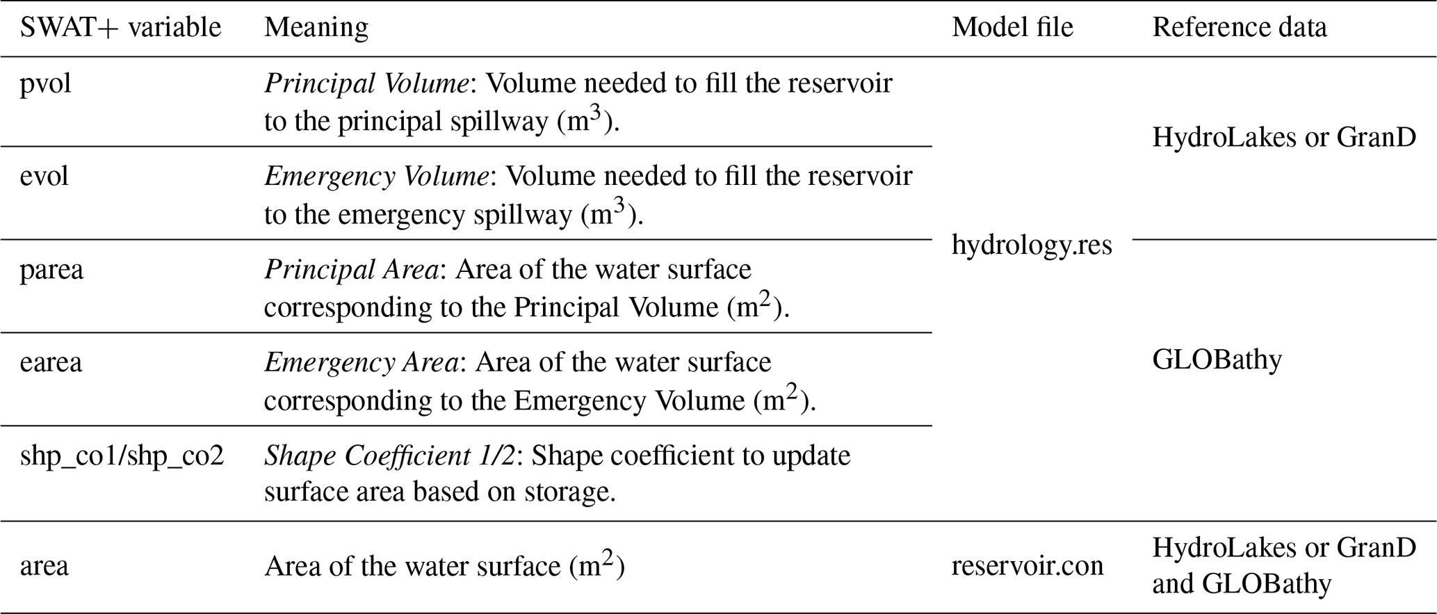
A summary of the datasets used in this study is provided in Table 1. This includes data on the setup of CoSWAT, the reservoir/lake simulation schemes, irrigation demand, and model evaluation. Datasets for model setup provide mappings of the physical properties of land and soil, which are essential for the creation of HRUs. The topography was defined using the Global Aster Digital Elevation Model (DEM; Abrams, 2016). The reference land cover map was obtained from the ESA CCI Land Cover Product (ESA, 2017), while soil classification and properties were derived from the FAO Harmonized World Soil Database (Fischer et al., 2008). These data were resampled from their native resolution to 0.01°, as shown in Table 1. Finally, the CoSWAT model requires daily precipitation, maximum and minimum temperatures, solar radiation, wind speed, and relative humidity as weather inputs, all of which are available in the GWSP3-W5E5 dataset (Lange et al., 2022) at 0.5°, and were used in this study to perform historical simulations.

Table 1 Datasets used in this study, resolution, purpose of use, and source.

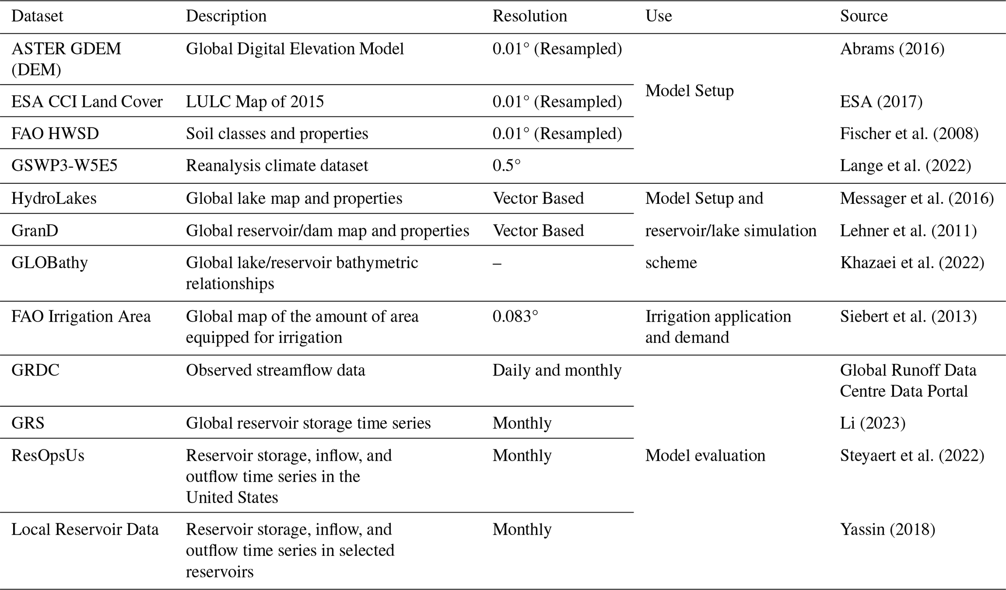
Some datasets were used both in the setup and in the configuration of the reservoir/lake simulation scheme. This includes the HydroLakes and GranD datasets, which were used to integrate lakes and reservoirs into the model's structure based on their geographic locations. The physical and operational properties, together with the depth–area–volume (h–A–V) relationships from the GLOBathy dataset, were used to establish the new reservoir/lake simulation scheme. Moreover, the FAO Irrigation Area dataset provided key inputs to identify irrigated HRUs, which were subsequently configured to represent irrigation application and demand. For model evaluation, data from the Global Runoff Data Centre (GRDC; https://grdc.bafg.de/data/data_portal, last access: 14 July 2026) were used to evaluate streamflow, and a combination of three data sources, GRS (Li, 2023), ResOpsUs (Steyaert et al., 2022), and (Yassin, 2018), was used to evaluate the model's storage, inflow, and outflow outputs under the new implementations.

2.2 Regions of application

The CoSWAT model is divided into 90 regions (Chawanda et al., 2025) representing one or more large river basins. For this study, 9 of those regions (Fig. 1), were selected to apply and evaluate the implementations developed in this study, spanning diverse environmental and operational conditions across nearly all continents, where sufficient data were available for robust evaluation. The selected regions span several climatic zones worldwide, including tropical, arid, temperate, cold, and polar (frost), according to the Köppen–Geiger classification system (Beck et al., 2023). In South America, the modelled region covers the La Plata, Parana and Endorheic Basins. In North America, the Mississippi River System, the Colorado River Basin, the Grande (or Bravo) River Basin, and the Pacific Ocean Seaboard. In Africa, it encompasses the Nile River and the Orange River basins. In Asia, it covers the Mekong River and Chao Phraya River basins. Finally, two model regions cover most of western and central Europe, encompassing several river basins.

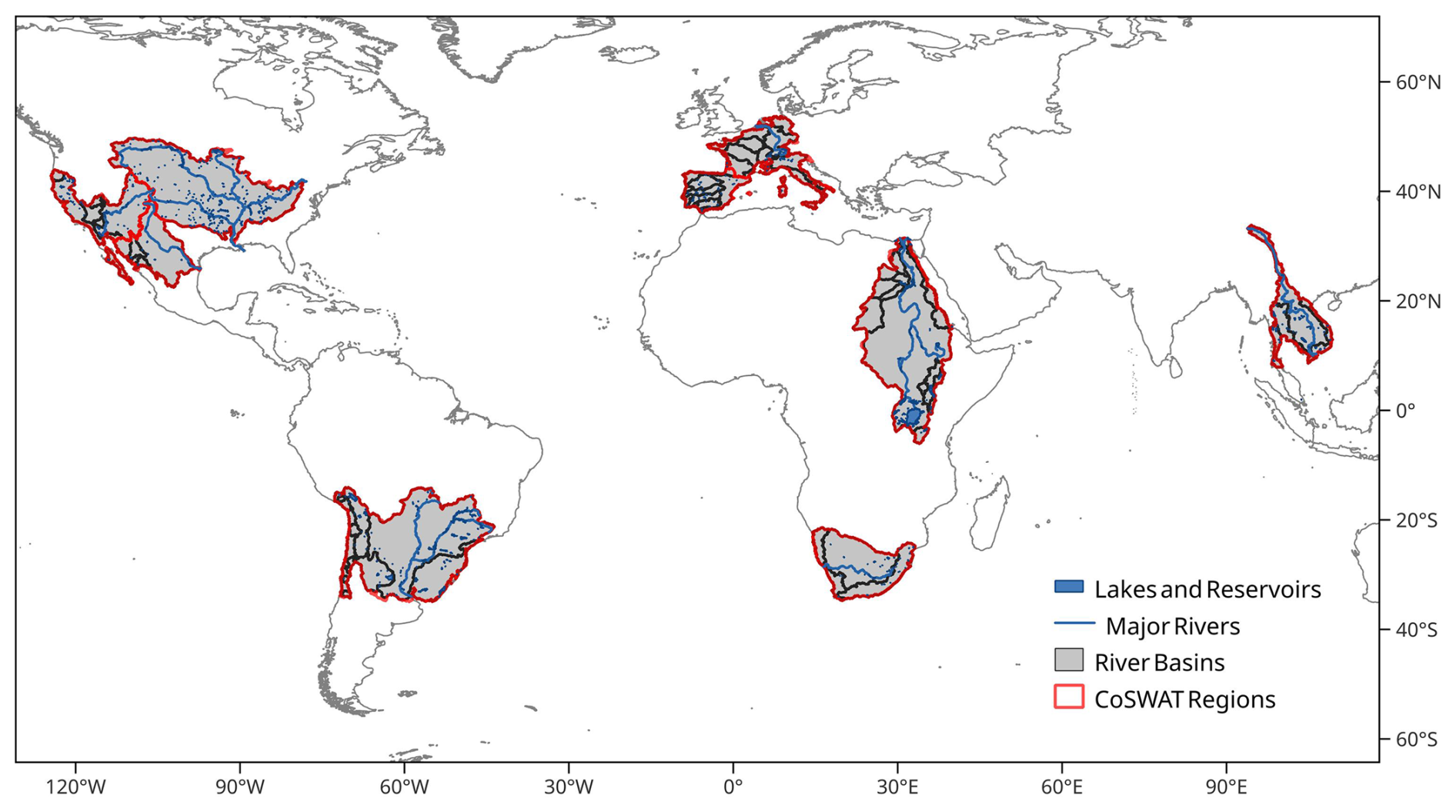
Figure 1 CoSWAT Model regions and River Basins of application for this study. Basin sub-division was done using the HydroBasins dataset (Lehner and Grill, 2013).

2.3 Reservoir/lake integration into model network

In SWAT+, model components are fully vectorized, and lakes or reservoirs are commonly integrated by intersecting their polygon geometries with the river network and spatial model units using GIS tools such as QSWAT+. In this approach, inlets and outlets are identified using geometric rules (e.g., by determining the reach endpoint location relative to the water body), HRUs are converted to water areas, and the model structure is adjusted accordingly. However, this procedure relies primarily on geometric criteria and does not explicitly account for river network topology, which can lead to ambiguous inlet/outlet classification and the exclusion of water bodies, particularly for complex geometries and coarse resolution river networks in global applications. To overcome these limitations, we integrated new steps into the CoSWAT framework (Fig. 2), which allows for an adequate integration of reservoirs and lakes into the model structure.

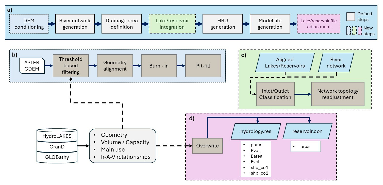
Figure 2 Overview of the (a) CoSWAT framework for model structure generation, with three new components introduced in this study: (b) DEM conditioning and preprocessing, (c) lake and reservoir integration into the network topology, and (d) adjustment of model files for reservoirs and lakes using global datasets (HydroLAKES, GranD, GLOBathy).

Table 2 Main hydrological reservoir variables in SWAT+.

The additions consist of a pre-processing stage (Fig. 2b), a lake/reservoir integration stage (Fig. 2c), and a model file adjustment stage (Fig. 2d). The preprocessing stage has three main steps: (i) threshold-based filtering of water bodies, (ii) alignment of channel-lake intersections to the DEM grid, which prevents the creation of river segments and HRUs smaller than the DEM grid cell, which is required for numerical stability in SWAT+, and (iii) burn-in of lake/reservoir geometries into DEM by 14 m following Lehner et al. (2008), and a depression correction (i.e. “Pit fill”) with the Whitebox Geospatial Analysis Tools (Lindsay, 2016), resulting in a conditioned DEM. After that stage, the river network and drainage areas are generated using the Terrain Analysis Using Digital Elevation Models (TauDEM; Tarboton et al., 2009) tool. With that information, the integration of water bodies into the network proceeds, and it consists of two steps: (i) logical identification of inlets and outlets and (ii) re-adjustment of network topological connections. For this study, water bodies smaller than 20 km² were excluded, except when the degree of regulation (i.e., ratio of storage capacity and mean annual outflow) provided by the GranD dataset exceeds 70 %, and the area exceeds 10 km². After the integration of lakes and reservoirs, the next step is to create the model's HRUs and model file generation.

Finally, the framework with the new steps generates the SWAT+ model files and populates reservoir-related variables (Fig. 2d) that cannot be inferred solely from vector geometry (Table 2), therefore relying on information from global datasets. The relevant files are “hydrology.res”, which contains numerical information used for calculations during simulation, and “reservoir.con”, which contains information about connectivity with other elements in the model. Each water body is classified as natural or regulated based on the HydroLakes dataset attribute “Lake type”. For unregulated lakes, properties related to storage are derived from data reported in HydroLakes. For regulated water bodies, this is taken from the GranD dataset. The GLOBathy dataset provides the exponential bathymetric coefficients for the depth–area–volume (h–A–V) relationships of each water body, enabling the determination of “shp_co1” and “shp_co2” coefficients. Finally, the GranD's attribute “Main Use” is stored in the model vector files for use in subsequent simulations (e.g., flood control, irrigation, hydropower, water supply).

2.4 New lake and reservoir simulation scheme

2.4.1 Water balance

The water balance for lakes and reservoirs in SWAT+ is as follows (Neitsch et al., 2011):

$$\begin{array}{}\text{(1)}& {\displaystyle \frac{\mathrm{\Delta }S}{\mathrm{\Delta }t}}=P+Q_{\mathrm{in}}-E-G-Q_{\mathrm{out}}\end{array}$$

where $\frac{\mathrm{\Delta }S}{\mathrm{\Delta }t}$ (m³ d⁻¹) is the change in storage per daily time step of the simulation, P (m³ d⁻¹) is the precipitation on the surface of the reservoir, Q_in (m³ d⁻¹) is the surface water inflow, E (m³ d⁻¹) is the evaporation from the water surface, G (m³ d⁻¹) is the seepage to or from groundwater, and Q_out (m³ d⁻¹) is the release from a regulated reservoir or the outflow from an unregulated lake. Precipitation is a direct input from weather forcings, whereas surface water inflow results from routing water through inlets that drain into the water bodies and from runoff of adjacent HRUs. However, evaporation, groundwater fluxes, and release or outflow need to be calculated during the simulation. Our approach maintains the existing methods to derive evaporation and seepage (Neitsch et al., 2011), as described in detail in Appendix A. By default, SWAT+ simulates outflow or release using decision tables (Arnold et al., 2018). We enhanced SWAT+ revision 61.0.2 by modifying reservoir-related subroutines and integrating decision tables with two parametric methods; one based on Döll et al. (2003) for natural lakes, and one based on the H06 scheme (Hanasaki et al., 2006) for regulated lakes and reservoirs, in order to improve global applicability, thereby supporting the CoSWAT GWM.

2.4.2 Unregulated lake outflow

To determine unregulated lake outflows, we divide the lake's storage into active and inactive. The threshold for separating active from inactive storage is set to the lake volume corresponding to a depth of 5 m, following Döll et al. (2003) for global applications, and is then expressed as a percentage of the principal volume. This is intended to maintain a minimum storage level in the lake at all times, thereby avoiding unrealistic drops; nonetheless, this is a rather arbitrary definition and may require fine-tuning for future applications, particularly in large lakes. The volume corresponding to that depth is determined using the GLOBathy h–A–V relationships. Based on this, the decision table is constructed, and the outflow is determined by the conditions. When the lake storage is above the active volume threshold, the outflow is based on the parametric, time-invariant method developed by Döll et al. (2003):

$$\begin{array}{}\text{(2)}& Q_{\mathrm{out}}=K_{\mathrm{r}}\cdot \left(S-s_{\mathrm{o}}\cdot \mathrm{pvol}\right)\cdot {\left({\displaystyle \frac{S}{\mathrm{pvol}}}\right)}^{\mathit{\alpha }}\end{array}$$

where K_r is a release coefficient, in this case fixed to 0.01 d⁻¹, S (m³) is the current storage in the simulation, s_o the active/inactive storage threshold coefficient, pvol (m³) is the established principal volume, in this case, derived from Hydrolakes, and α is an exponential coefficient set to 1.5. On the other hand, if the storage is below the inactive/active volume threshold, the outflow is simply zero.

2.4.3 Regulated lake and reservoir release

The release simulation scheme for regulated water bodies is a decision table with multiple release approaches. Central to the approach is a parametric, time-variant method, based on the H06 reservoir scheme (Hanasaki et al., 2006) and different implementation approaches (Gharari et al., 2024; Vanderkelen et al., 2022). The H06 scheme distinguishes between irrigation and non-irrigation reservoirs, and its formulation differs accordingly. The key to its approach is defining a release target and actual release based on past inflows and/or irrigation demands, reservoir properties, and the simulated storage at each time step. A detailed description of the method and its implementation in the CoSWAT model is provided in Appendix A.

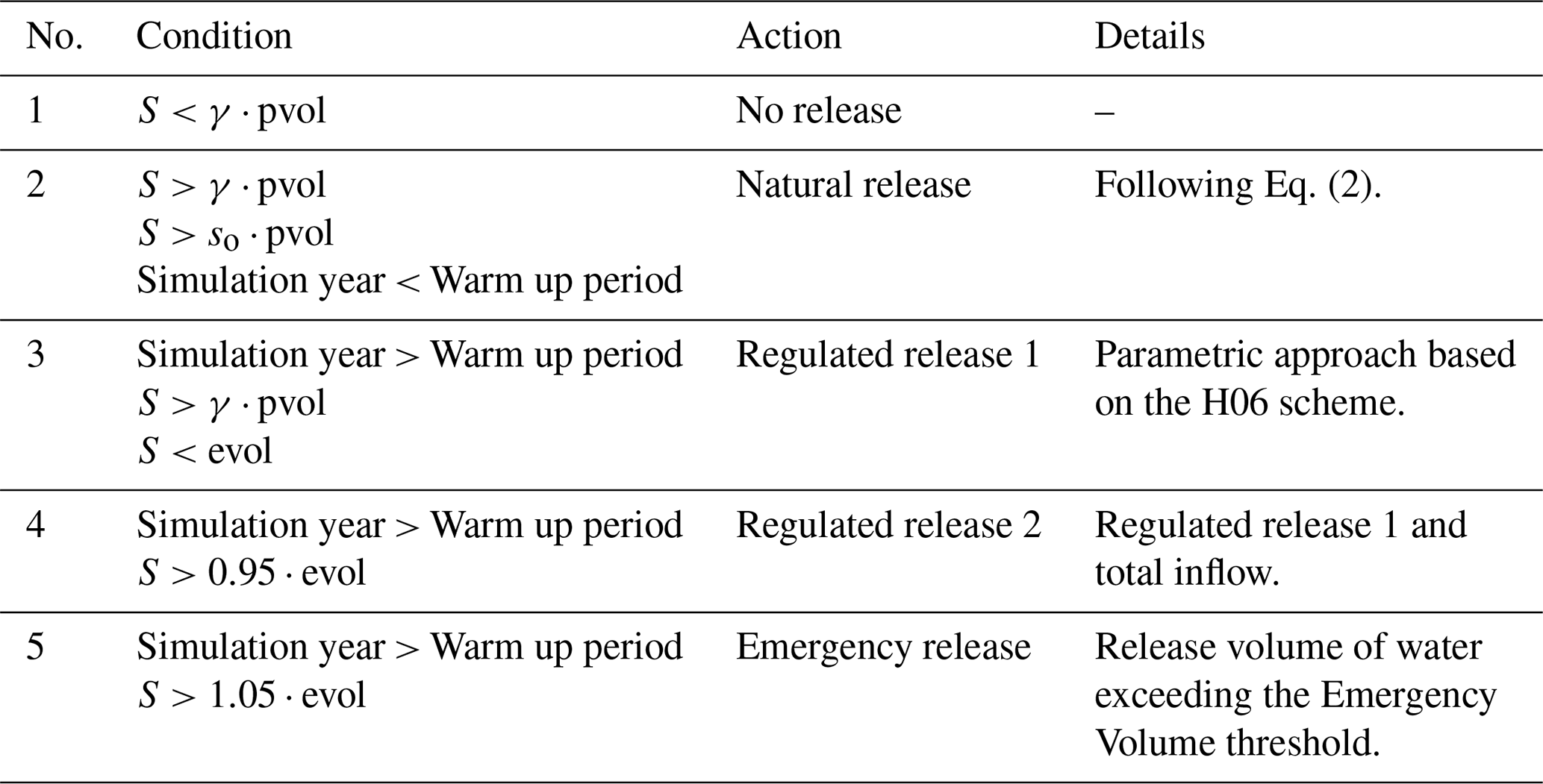
As shown in Table 3, the decision table for a regulated water body comprises five conditions at each daily time step. First, the Υ coefficient serves as a threshold that prevents release when reservoir storage falls below this value, thereby ensuring availability during dry months. For this application, Υ was set to 0.15. The second condition applies only during the simulation's warm-up period, during which all water bodies are modeled as natural lakes. This is done to generate historical inflow and irrigation demand data that will subsequently feed the used scheme. For the remainder of the simulation, under the third and fourth conditions, in which reservoir storage is maintained below emergency levels, the downstream release of regulated water bodies is estimated using the parametric H06 scheme. However, as the storage approaches the emergency level (>95 %), the release is increased to delay the accumulation of storage. Under the fifth condition, if reservoir storage exceeds 5 % of the Emergency Volume, the entire volume above that threshold is released.

Table 3 Decision table structure for regulated reservoirs. S: Storage, pvol: Principal volume, evol: Emergency volume, γ: Reservoir minimum storage coefficient.

2.5 Irrigation application and demand

The introduction of irrigation application and demand is highly relevant for more accurately representing water management practices in the model. It is also required to fully implement the reservoir/lake simulation scheme for irrigation reservoirs, which require information on downstream irrigation demand to determine their releases. This process was divided into three steps: (i) the definition of irrigated HRUs, (ii) the definition of the source of irrigation water via an irrigation topological connection between model elements, and (iii) the generation of land use management decision tables and the modification of relevant model files. This procedure was also integrated into the CoSWAT Framework to automatically define irrigation for the modelled regions.

The FAO area equipped for irrigation maps is divided into surface-water and groundwater sources. These maps were overlaid with HRUs classified by agricultural land use, and HRUs with an irrigation area fraction exceeding a specified threshold were designated as irrigated. For the regions applied in this study, the threshold was set to 40 %, after which the irrigation water source was identified for irrigated HRUs (Fig. 3). First, whether HRUs used surface or groundwater was based solely on the FAO area equipped for irrigation maps. If an HRU overlaid areas with both sources, the dominant percentage of the equipped area was used as the primary source. To further establish surface water demands for irrigation-purpose reservoirs, a topological connection process was performed following Vanderkelen et al. (2022). This process was used to identify HRUs that require water from an irrigation reservoir. The approach considers the river network downstream of the reservoir outlet for up to 1000 km, encompassing the main river and its tributaries up to second-order. An irrigated HRU with surface water as the primary source, that is hydrologically connected to that portion of the river network, and whose mean elevation is below the mean elevation of the corresponding reservoir, is considered to demand irrigation water from the reservoir. If an HRU demands irrigation water from two or more reservoirs, the demand is weighted to each reservoir based on the ratio of that reservoir's maximum storage capacity to the sum of the maximum storage capacities of all associated reservoirs.

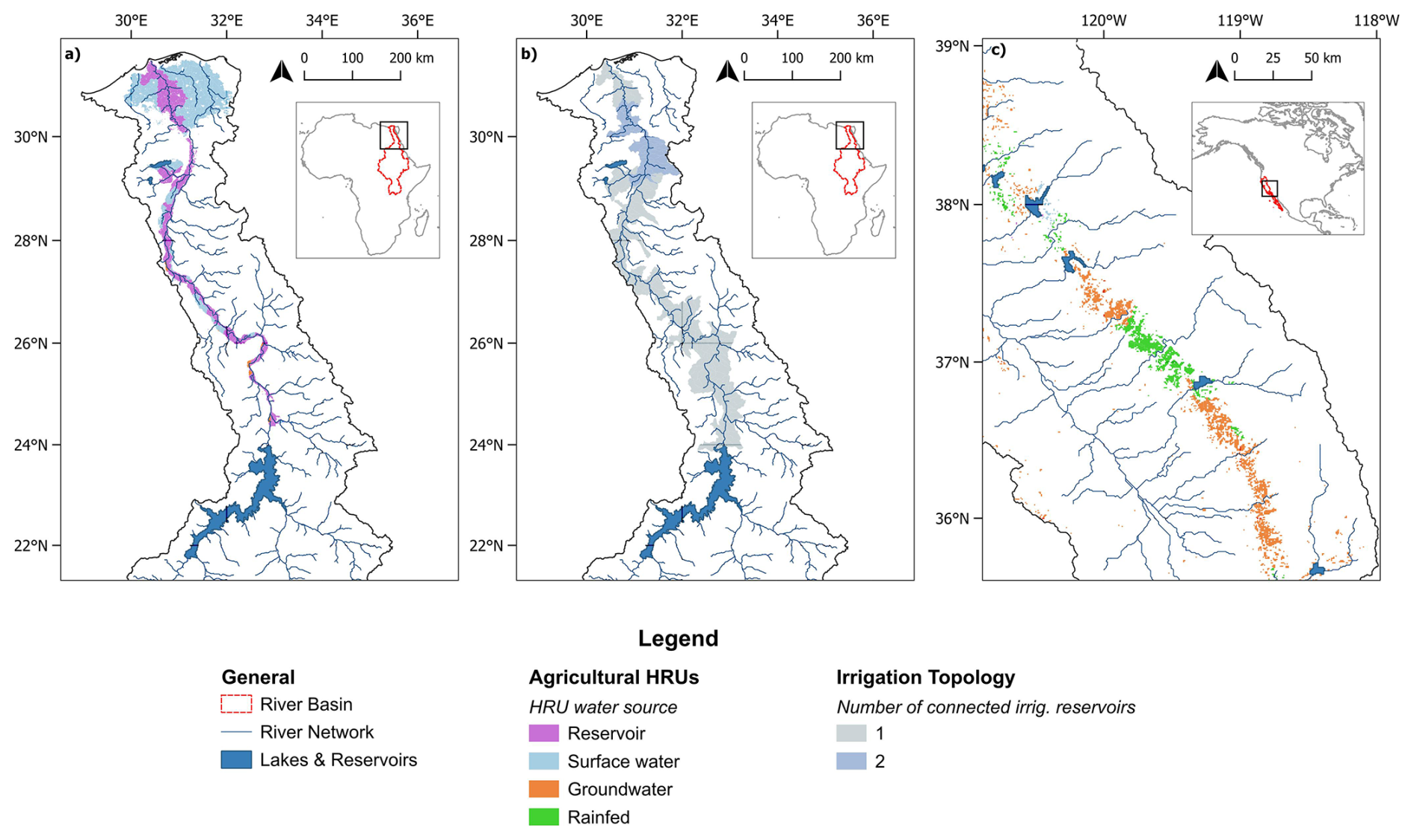
Figure 3 Irrigation water source assignment for agricultural HRUs and irrigation topology, illustrated for two contrasting regions: (a) a predominantly irrigated downstream section of the Nile River Basin, (b) the corresponding irrigation topology showing the number of connected irrigation reservoirs per sub basin, and (c) a section of the Pacific Seaboard in North America, where agricultural HRUs rely predominantly on groundwater or are rainfed.

Finally, land use management decision tables were established for each identified HRU. For irrigated HRUs with a groundwater source, irrigation water was allowed to be extracted from the shallow aquifer. For those with a surface-water source, water was extracted from the nearest river to the HRU. In all cases, irrigation is applied based on a water-stress threshold rather than a fixed calendar. For those that require water from a reservoir, an additional land use management action was implemented in the SWAT+ source code to record reservoir irrigation water demand. This means that water is not directly extracted from the reservoir; only the demand is recorded, which influences the reservoir's release.

2.6 Simulation setup, model comparison, and evaluation

The model was configured for the 9 selected regions using spatial input data at 0.01° resolution, finer than the 0.02° resolution of CoSWAT v1 (Chawanda et al., 2025). The weather forcings were derived from the GSWP3-W5E5 dataset, and the simulations were conducted using the adjusted version of SWAT+ (revision 61.0.2) at a daily time step for the period 1965–2015, with a 5-year warm-up. The initial storage for all water bodies was set to their principal volume. The model outputs were evaluated using Kling–Gupta Efficiency (KGE), percent bias (PBIAS), and coefficient of correlation (r) for both streamflow and reservoir storage, as well as inflow and outflow. To assess model adequacy, thresholds were defined for these statistical performance/error indicators. Given that this is a large-scale application with coarse input data, the minimum acceptable KGE value was set to −0.42, which represents a better performance than just taking the mean of the observations (Knoben et al., 2019). However, the objective value for satisfactory performance was set at a minimum KGE of 0.0, with 0.4 considered good performance, and this was similarly applied to r. The PBIAS threshold and objective were set to ±50 % as satisfactory, and ±25 % as good (Moriasi et al., 2007).

2.6.1 Reservoir storage, inflow, and outflow

The model version with new implementations was evaluated for its ability to represent the monthly means of reservoir storage, inflow, and outflow. For this, the GRS (Li, 2023), ResOpsUs (Steyaert et al., 2022), and selected data by Yassin (2018), as summarized in Table 1 was pre-processed and aggregated. Only reservoirs with at least 5 years of at least 1 data point and 1 year of continuous storage data were considered, then aggregated across sources. If a reservoir had multiple data sources, the average value was used as the reference.

To place model performance in a broader context, monthly reservoir storage was compared against five state-of-the-art global water models from the ISIMIP Global Water Sector (Gosling et al., 2024): CWATM (Burek et al., 2020), H08 (Hanasaki et al., 2018), LPJmL5-7-10-fire (Wirth et al., 2024), MIROC-INTEG-LAND (Yokohata et al., 2020), and WaterGAP2-2e (Müller Schmied et al., 2024). All models were evaluated using simulation outputs driven by observationally based GSWP3-W5E5 climate forcing and historical human-socioeconomic forcings for the same period as this study. ISIMIP outputs are provided on a common 0.5°×0.5° grid, where each cell represents aggregated water storage from all lakes and reservoirs within that cell (i.e., representative water body). For each evaluated reservoir, the storage time series was extracted at the grid cell corresponding to the reservoir outlet. This differs from CoSWAT, whose outputs are not gridded and are produced explicitly for each water body. Where multiple reservoirs/lakes fell within the same grid cell, their contributions were proportionally weighted using their maximum recorded volume from the HydroLakes dataset. If the sampled grid cell from the ISIMIP models produced a time series of persistent zero storage, the reservoir was assumed not to be represented in that model and was excluded from further analysis.

2.6.2 Streamflow

To assess the impact on streamflow performance, the model was configured with and without the new implementations, yielding one version for each region that included lakes, reservoirs, and irrigation, and another that excluded them. What is important about this evaluation, is that the CoSWAT model has not been calibrated (Chawanda et al., 2025), so the simulations were conducted with default parameter values for relevant hydrological processes and river routing. Monthly streamflow performance, using GRDC data as the reference, was compared between the two versions at stations downstream of a lake or reservoir significantly impacted by new implementations, i.e., the absolute KGE skill score (Towner et al., 2019) is above 0.05 following Eq. (B1). Performance thresholds were used to assess how the new implementations affect model performance, with particular emphasis on the KGE metric. Based on them, four categories were established for comparison:

• Category 1: performance without implementations is satisfactory (KGE > 0) and new implementations increase KGE.

• Category 2: performance without implementation is not satisfactory (KGE < 0), and new implementations increase KGE.

• Category 3: performance without implementations is satisfactory (KGE > 0), and new implementations decrease KGE.

• Category 4: performance without implementations is not satisfactory (KGE < 0), and new implementations decrease KGE.

This evaluation helps identify where improvements occur or do not, and to what extent, which is especially useful when examining categories 2 and 3, as crossing the satisfactory threshold is possible. Those in category 1 represent locations where the model alone performs satisfactorily, but the new implementations further increase its reliability. In contrast, those in category 4 represent locations where poor performance has already occurred; the new implementations are initially counterproductive, while other factors are more influential and potentially more relevant for improving model performance.

3 Results

3.1 Lake and reservoir integration into model structure

The new reservoir and lake integration process implemented in the CoSWAT-Framework integrated 498 reservoirs or lakes into the model structure for the study regions, out of 632 possible (excluding those filtered out by the initial area and degree of regulation thresholds), yielding an efficiency of 79 %. Nonetheless, considering the maximum storage capacity or representative storage based on global datasets, the integrated water bodies account for 2992 km³ of storage out of 3286 km³, representing 91 % of the total storage.

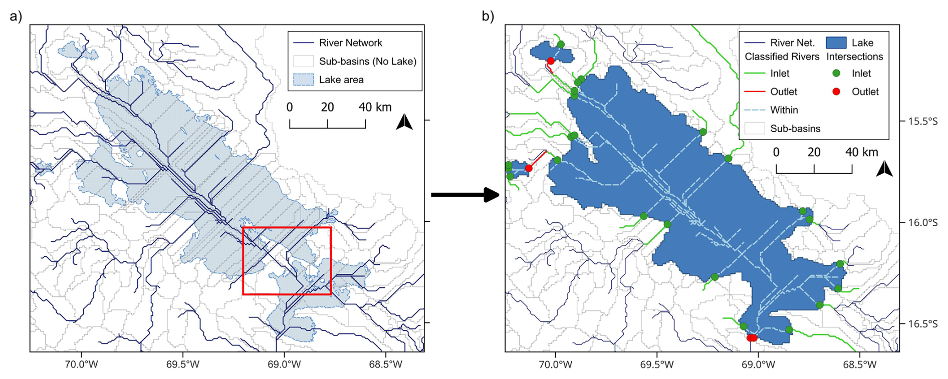
Figure 4 Example of Lake Titicaca in the model structure, (a) before network integration process, and (b) after integration, showing classified river network elements and points of intersection at the water body limits to define inlets and outlets. Rivers classified as “Within” are eventually excluded from the model structure. The area marked in red on box (a) represents the Lago Menor division, an example where complex topography leads to a network in which the lake cannot be integrated without the new integration approach.

Figure 4 shows one of the complex cases where the CoSWAT Framework would typically fail to integrate a water body into the model structure, as only river endpoint geometrical rules are not sufficient, and require a more robust approach considering network topology: Lake Titicaca, which has complex locations such as the Lago Menor division (highlighted area, box a). The resolution process simplified the geometry in the vector file. However, physical properties related to area, storage, and h–A–V relationships remain correctly represented in the model, as global dataset values are introduced in the simulation model files. This is one of many cases that showcase how the new integration approach enables more efficient integration of water bodies.

3.2 Reservoir and lake storage, inflow and outflow evaluation

A total of 215 water bodies were evaluated for monthly storage, with results summarized in Figs. 5a and B1. In terms of KGE, 150 (70 %) achieved a value above the minimum threshold (-0.42); however, only 73 (34 %) achieved a positive KGE value. The distribution is approximately normal, with a median of −0.1; however, it has a long tail toward negative values, indicating fewer cases with very poor performance. Moreover, for 94 cases (44 %), PBIAS was between the good ±25 % range. Overall, the PBIAS distribution for storage is wide and moderately asymmetric, with extended tails toward both large negative and positive values, but with a stronger tendency toward overestimations. The correlation coefficient was positive in 153 cases (71 %), with 48 stations (22 %) achieving a good performance (r>0.4). A large proportion of stations fall within the intermediate range (0–0.4), indicating moderate but not consistently strong model performance across sites.

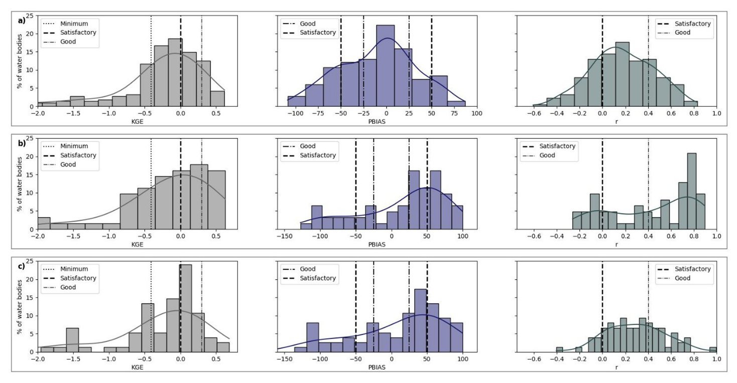
Figure 5 Distribution of KGE, PBIAS, and R related to model performance for monthly mean (a) storage, (b) inflow, and (c) outflow, using normalized histograms expressed as a percentage of evaluated water bodies for the corresponding variable. A kernel density estimate (KDE) curve is overlaid on each histogram to provide a continuous representation of the underlying probability distribution. Vertical reference lines indicate the established adequacy classifications for performance thresholds.

Monthly inflow performance was assessed for 62 water bodies, and outflow for 75 (Fig. 5b and c, respectively). For inflow, in 44 cases (71 %), the minimum KGE threshold was exceeded, but fewer than half (28 sites) achieved a positive value. The inflow KGE distribution is centered near zero, with a long tail toward very poor performance. Only 11 cases (18 %) had inflow PBIAS in the satisfactory range; there is widespread over- and underestimation, with a high concentration of cases around moderate positive biases and a significant number of important overestimations. Outflow performance is generally similar: 49 sites (65 %) exceed the minimum KGE threshold, but only 27 achieve a positive KGE. Outflow shows even greater PBIAS variability, driven mainly by several extreme biases. Correlation is predominantly positive for both variables, but consistently higher for inflow (60 % of stations above 0.4) than for outflow (33 % above 0.4), suggesting that the model generally captures inflow timing better than outflow timing.

To further explore the drivers of storage performance, relationships among storage metrics, inflow/outflow skill, and water body characteristics were analyzed (Fig. B2). Storage KGE shows a moderate to low, statistically significant positive relationship with inflow and outflow KGE (r≈0.35–0.38), indicating that improved representation of inflows is associated with better storage and outflow performance, particularly for reservoirs exceeding the minimum skill threshold for storage (KGE > −0.42). A similar pattern is observed for inflow timing: higher storage performance is associated with higher inflow correlation (r≈0.39), suggesting that improvements in the temporal representation of inflows yield more realistic storage dynamics. In addition, storage PBIAS shows a moderate-to-low relationship with elevation (r≈0.32). However, while a clear cluster of low-elevation reservoirs (below 500 m a.s.l.) exhibits substantial negative storage PBIAS (Fig. B2c), driving the observed elevation relationship, inflow and outflow PBIAS show no statistically significant relationship with elevation nor correspondence with this cluster (Fig. B2d). Further investigation of this cluster reveals three factors behind it; two representative examples are shown in Appendix B (Fig. B3). First, the reference storage capacities from GRanD and HydroLAKES, used to initialize and parameterize the simulation scheme (Fig. B3a and b), substantially exceed the harmonized reference validation data (Table 1), causing simulated storage to fluctuate near this elevated capacity rather than at the observed levels. Second, in some cases, the reference validation data itself shows important variability across sources, increasing evaluation uncertainty (Fig. B3a). Third, some cases in this cluster have significantly underestimated inflows, which, combined with the parameterization, lead to inaccurate outflows and keep storage near the prescribed maximum capacity with limited fluctuation, leading to the negative values of PBIAS.

To further illustrate the representation of reservoirs and lakes, Fig. 6 compares simulated and reference storage, inflow, and outflow for four water bodies with sufficient data availability on different orders of magnitude in terms of their storage capacity. Overall, storage representation is generally adequate in magnitude, though with some temporal deviations, while inflow and outflow performance varies among them. Fort Berthold reservoir (Fig. 6a) and Lake Oahe (Fig. 6b) are two cascading reservoirs upstream on the Mississippi River system, primarily operated for flood control. Fort Berthold shows overestimated inflows and, consequently, outflows for much of the simulation period, which propagate downstream to Lake Oahe, where similarly overestimated outflows occur, generally causing significant storage fluctuations. During 2004–2009, storage overestimation was persistent, mainly driven by inflow overestimation that exceeded outflow overestimation. These two reservoirs illustrate two important situations: the propagation of errors through cascading reservoir systems, and cases where storage magnitude is reasonably captured but is subject to significant fluctuations due to overestimation of inflows and outflows.

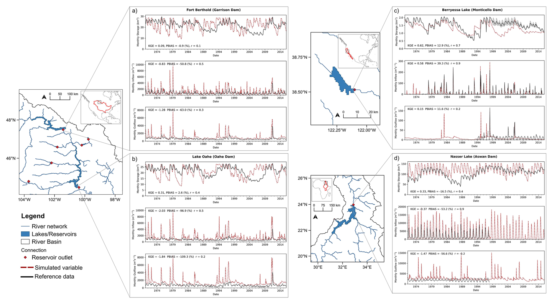
Figure 6 Simulated and reference data comparison for monthly storage (top), monthly inflow (middle), and monthly outflow (bottom) for four selected reservoirs: (a) Fort Berthold, (b) Lake Oahe in the Mississippi River system, (c) Berryessa Lake in the Sacramento River Basin, and (d) Nasser Lake in the Nile River Basin. Shaded areas in storage indicate periods with multiple observational sources differing in absolute value.

Berryessa Lake (Fig. 6c) is a regulated water body mainly used for hydroelectricity, and shows one of the best overall performances: storage is well reproduced except for notable underestimation during 1999–2004 and 2006–2014. The first period is preceded by a large, overestimated outflow peak in 1998, causing an abrupt storage decline; thereafter, underestimated inflows combined with overestimated low-season outflows prevent recovery to observed levels. Storage recovers by 2006, but a subsequent high inflow peak triggers renewed outflow overestimation, returning storage to underestimated levels. This case illustrates how punctual but significant over- or underestimations of outflow can substantially affect storage representation for several years.

Finally, Lake Nasser (Fig. 6d) is an irrigation-oriented reservoir, where storage is often overestimated and its variability exaggerated. Moreover, in the period 1984–1994, a significant drop in storage was not captured. Although inflow timing is relatively well represented, magnitudes are generally too high, while outflow is both overestimated and temporally shifted. Based on reference data and other reports (Abdellatif et al., 2025), the Aswan Dam in Nasser Lake releases up to 60 km³ yr⁻¹, mainly for irrigation. Throughout the year, the model tends to overestimate the release, yet the simulated irrigated amount downstream averaged 7–10 km³ yr⁻¹, indicating a substantial underestimation of irrigation demand. Hence, the effect of overestimating runoff in this basin, therefore, inflow to the reservoir is dominant despite possible underestimation of demands.

3.3 Comparison with other global models

As an additional benchmark for the storage evaluation, performance results were compared with five global water models from the ISIMIP Global Water Sector (Fig. 7). Across these models, the number of reservoirs evaluated varies widely, from 65 for CWATM to 195 for LPJmL5-7-10-FIRE, with intermediate sample sizes for H08 (78), MIROC-INTEG-LAND (183), and WaterGAP2-2e (96). In contrast, CoSWAT results encompass 197 water bodies, effectively covering the union of those represented across all models. These differences arise because grid cells with all-zero storage time series were excluded, suggesting that the reservoir with observed data is not represented in the model or that the sampled pixel does not precisely match its location. It is important to note that Fig. 7a shows violin plots computed using only the subset of water bodies simultaneously represented by CoSWAT and each respective ISIMIP model. As a result, the CoSWAT distribution differs across comparisons, since the sample varies per model pair rather than always reflecting the full set of 197 reservoirs. The bar charts in Fig. 7b, in contrast, report the proportion of water bodies exceeding performance thresholds normalized by the total number of reservoirs represented by each model, thereby reflecting overall coverage and skill. Inter-model comparisons should be interpreted as indicative benchmarks relative to CoSWAT rather than definitive global performance assessment of the five ISIMIP Global Water models.

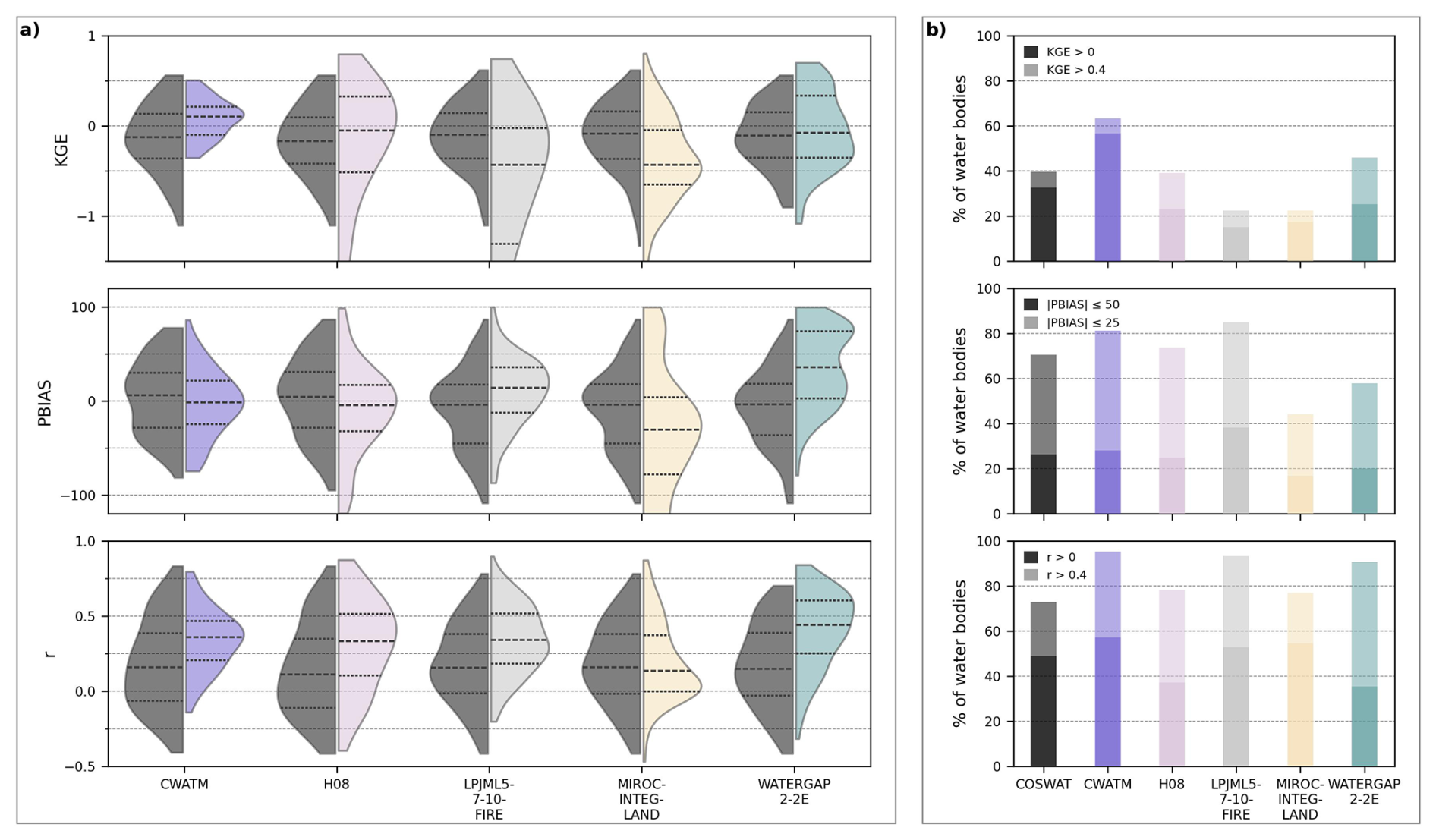
Figure 7 Performance comparison for mean monthly storage representation between CoSWAT with new implementations and five ISIMIP Global Water Sector models. Box (a) shows violin plots with the KDE distribution of CoSWAT (left panels) and the other models (right panels) for KGE, PBIAS, and r, considering only the water bodies available in the ISIMIP reference model. A dashed line represents the median, while dotted lines represent the first and third quartiles. Box (b) shows, for each model, the percentage of water bodies exceeding the “satisfactory” and “good” performance thresholds for KGE, PBIAS, and r, normalized by the total number of reservoirs represented by that model. For each model, the lighter shade corresponds to the “good” threshold and the darker shade to the “satisfactory” threshold. Outliers were not considered.

Overall, the models show broadly comparable storage skill, as indicated by median KGE values clustering from weakly negative to slightly positive. CWATM obtains the highest median KGE (0.10), followed by WaterGAP2-2e (−0.08), and H08 (−0.11), while MIROC-INTEG-LAND (−0.44), and LPJmL5-7-10-FIRE (−0.56) exhibit progressively lower medians, below the −0.42 threshold. For the 197 water bodies, CoSWAT achieves a median KGE of (−0.08), although this varies by subset with direct comparisons. The violin plots reveal variability across all models, with notable differences in spread: CWATM shows the most compact interquartile range and KDE curve, whereas LPJmL5-7-10-FIRE and H08 display broader distributions with long tails towards negative KGE values. CoSWAT, WaterGAP2-2e, and MIROC-INTEG-LAND are comparable in their variability, which is somewhat moderate. However, the two former show interquartile ranges centred on higher KGE values than the latter. Regarding performance thresholds, CWATM has the highest number of water bodies with satisfactory KGE (62 %), followed by WaterGAP2-2e (44 %), CoSWAT and H08 (both ≈40 %), with the rest below 25 %. WaterGAP2-2e and H08, however, achieve the highest proportion of water bodies with a “good” performance (KGE > 0.4) with approximately 20 % and 16 %, respectively, while for the rest, this is below 10 %. For PBIAS, CWATM, CoSWAT (across 197 bodies), and H08 are closest to zero (median PBIAS of −1.2 %, −3.9 %, and −4.1 %, respectively), whereas MIROC-INTEG-LAND and WaterGAP2-2e display much stronger median biases (−30 % and +36 %), indicating a general over- or under-estimation. The PBIAS distributions are broad across all models, particularly for MIROC-INTEG-LAND, which exhibit extensive ranges and multiple extreme values. The PBIAS KDE curve is relatively centred around zero for CWATM, H08, and CoSWAT, in contrast to the others, though it remains spread. Most models achieve satisfactory PBIAS at at least half of the stations, except for MIROC-INTEG-LAND, which achieves only about 43 %. For the coefficient of correlation, WaterGAP2-2e achieves the highest median value (0.43), followed by CWATM (0.35), LPJmL (0.34), and H08 (0.30), while CoSWAT (0.16) and MIROC-INTEG-LAND (0.13) show weaker correspondence in temporal variability. The distribution of r for CoSWAT shows a large proportion above 0; the density is high around values below 0.2, and it also has the lowest proportion of water bodies with an r value above 0.4 (73 %).

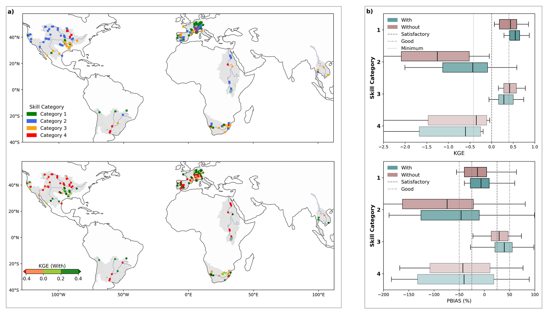
Figure 8 Monthly streamflow performance assessment. Box (a) shows the spatial distribution of stations with their corresponding skill category (top panel) and the KGE value of the model with new implementations (bottom panel). Box (b) shows the distribution of performance per skill categories for KGE (top panel) and PBIAS (bottom panel) with and without new implementations, as well as the performance classification thresholds.

3.4 Streamflow evaluation

A total of 192 stations were identified as significantly affected by the new implementations, and model performance was evaluated for these stations both with and without the new implementations. Across all stations, the median KGE increased from −0.07 to 0.05 following the new implementations. The number of stations with a good performance increases from 49 (25 %) to 58 (30 %), while the number of stations with satisfactory performance (KGE > 0) slightly reduces (44 to 40), and the stations surpassing the −0.42 threshold increase from 23 (12 %) to 32 (17 %). Overall, following the new implementations, the percentage of stations that meet the minimum threshold increases from 60 % to 68 %. In terms of PBIAS, the median value is reduced from −24 % to −16 %, and the number of stations within the satisfactory range (±50 %) increases from 50 (26 %) to 57 (29 %). The coefficient of correlation was above 0.4 at 152 (87 %) stations with new implementations, compared with 159 (85 %) without them. The observed changes based on the number of stations within a certain threshold are sometimes modest, highlighting the importance of looking at them in terms of the absolute change in performance indicators within their corresponding skill category (Fig. 8). Most stations fell into categories where skill increased with new implementations: 80 stations (42 %) were initially poor and improved (Category 2), and 53 (28 %) were already acceptable and improved further (Category 1). Conversely, 19 stations (10 %) declined in skill from an initially poor state (Category 4), and 40 (20 %) showed reduced skill despite initially acceptable performance (Category 3). Only a small fraction of stations crossed the KGE sign: 11 stations in Category 2 flipped from negative to positive, while 6 in Category 3 flipped from positive to negative. Regarding the minimum threshold (KGE > −0.42), 19 stations in Category 2 crossed above this limit, whereas only 2 in Category 3 crossed below it; 49 stations in Category 2 remained below the threshold, clearly showing that improvements achieved by the current integration of reservoirs and lakes are not directly leading to surpassing performance thresholds in most stations.

Spatially (Fig. 8a), Category 3 stations cluster in the lower Mississippi River system, particularly in downstream reaches with extensive drainage areas, reflecting the trade-off associated with new implementations; however, in most of these stations, performance remains above satisfactory levels. A very common situation is what can be observed in the upper Mississippi River System, overall in the Colorado River Basin, Nile River Basin and most sections of Western Europe: many stations are improving (Category 2), yet their KGE value remains below the minimum threshold, a clear indication that new implementations alone are not sufficient to take performance to satisfactory levels, but an improvement is indeed achieved. In Central Europe, a large number of stations are classified as Category 1 or 2, and, as with the stations mentioned earlier, most of those in Category 2 remain below the satisfactory threshold. In this region, there is also a small number of Category 3 and 4 stations, with the former remaining satisfactory in KGE despite reductions. The La Plata and Titicaca River Basins in South America have relatively few observations compared with the aforementioned regions, and the results vary significantly. There, upstream areas are generally improving and achieving good performance. The La Plata river basin's downstream stations, which were performing poorly without reservoirs, remain poor and classified as Category 4. In the Orange Basin of southern Africa, results are generally varied, and categories are distributed equally. What is clear on the Orange River Basin is that although some stations continue to perform poorly, the majority of mid- and downstream stations achieve satisfactory levels, with a mix of improvements and reductions in KGE. The Mekong River Basin has the fewest affected stations, classified as Category 3 and Category 1; the majority remain above satisfactory levels following implementation.

The box plots (Fig. 8b), indicate that stations that were already performing well show an important improvement (Category 1), with a positive shift in the median for both KGE and PBIAS, leading to a majority of stations achieving good performance and a better PBIAS. The KGE distribution for stations in Category 3 shows that, despite reductions, the majority remain satisfactory; however, with respect to PBIAS, there is a general shift towards large positive values, indicating a tendency to overestimate (i.e., likely to over-represent reservoir regulation). Category 2 shows the largest changes, with a substantial increase in the mean KGE from −1.3 to −0.43 and a distribution generally closer to satisfactory levels, although, as noted earlier, still with a majority below the desired values. In this category, there is a clear tendency to overestimate, with the PBIAS distribution concentrated in negative PBIAS values; this tendency is mitigated by recent implementations, which shift the mean toward the satisfactory range. Nevertheless, this highlights that the underlying issue leading to poor performance at these stations may be an overestimation of surface runoff, present even without reservoir implementation, and therefore related to hydrological parameter calibration rather than the reservoir integration itself. Finally, we observe a significant reduction in Category 4 stations, with KGE decreasing further and the PBIAS distribution expanding.

To illustrate how reservoir implementation affects streamflow behavior, six representative stations were selected to capture the range of positive and negative responses, choosing those with the largest KGE change within each category and a clear, interpretable effect (Fig. 9). Almourol station (Tagus river, ∼66 000 km²) falls in category 1, with several hydropower (e.g., Castelo do Bode, Alcantara) and irrigation (e.g., Valdecanas) reservoirs upstream. Performance improved mainly through better representation of dry-season flows, which were heavily underestimated without reservoirs. Calacoto station (Desaguadero river, ∼65 000 km²) shows a similar pattern, here driven by the downstream influence of Lake Titicaca (∼8300 km² surface area), whose regulating effect was absent in the simulation without the new implementations.

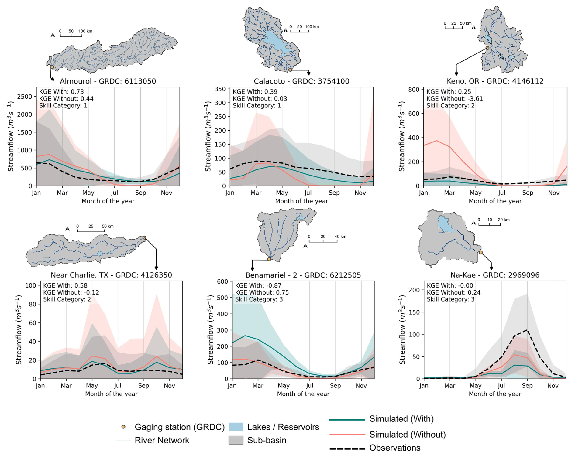
Figure 9 Seasonal monthly streamflow patterns for six selected GRDC stations, contrasting simulations with and without new implementations, and their respective sub-basin, upstream river network and presence of lakes or reservoirs. Lines show the mean monthly flow across the analysis period, while shaded bands denote ±1.5 SD (standard deviations). Titles indicate the GRDC station name and ID.

Keno (Klamath River, ∼18 000 km²) and Near Charlie (Wichita River, ∼8900 km²) both fall in category 2, showing significant performance improvements. At Keno, the absence of upstream reservoirs, including the regulated Upper Klamath Lake and the Clear Lake irrigation reservoir, leads to a strong overestimation of streamflow that largely disappears once they are included. Near Charlie presents a similar overestimation issue. While the mean climatology appears adequate, the shaded uncertainty band reveals substantial interannual overestimation, reduced considerably after introducing two upstream irrigation reservoirs, including Lake Kemp Dam. In contrast, the two Category 3 stations in Fig. 9 illustrate cases where reservoir introduction degraded performance. At Benamariel (Esla River, ∼4000 km²), overestimated outflows from an upstream irrigation reservoir amplify simulated streamflow, worsening model performance. At Na Kae (Lam Nam Kam River, ∼2400 km²), the regulation of Nong Han Lake exaggerates an existing underestimation, further suppressing flows that were already too low without reservoirs. In both cases, the current parametrization of the outflow calculation scheme likely drives over- or underestimation of target release and release coefficients, propagating errors downstream.

4 Discussion

4.1 Lake and reservoir integration into the model network

The representation of lakes and reservoirs in the SWAT+ model structure posed a topological challenge that was successfully addressed through improvements to the CoSWAT Framework, making it now feasible for the global CoSWAT model. Complex cases with multi-branch connections, lake or reservoir chains, and ambiguous connectivity were addressed correctly. The Lake Titicaca example illustrates this: a large water body with many inlets that acquires a complex geometry due to division into the Lago Menor section, which, through our process, was successfully added to the model network. Our topology-aware, robust approach, leveraging upstream-downstream connectivity and intersection logic, provided a consistent way to identify inlets and outlets and to adjust the routing network accordingly. Across the 9 model regions studied, satisfactory performance was achieved in feature integration and the hydrologic relevance of these water bodies. About 79 % of candidate water bodies across all regions were successfully integrated into the network. More importantly, 91 % of the total storage was represented, something as important as just the number of features, as larger water bodies will generally have a stronger influence on the basin's hydrology because of their high degree of regulation and evaporation rates (Shrestha et al., 2024; Zhao and Gao, 2019), particularly in the global context of this study.

4.2 Model performance of simulated reservoirs and lakes

Overall, reservoir and lake storage performance shows moderate skill, with substantial variability across river basins, as expected for large-scale models under generalized parametrizations and, as in CoSWAT, with uncalibrated parameters. Based on our comparison with other global water models, and the range of performance reported in similar large-scale evaluations (Hosseini-Moghari and Döll, 2025; Tang et al., 2025; Vanderkelen et al., 2022), the obtained storage skill is broadly comparable in magnitude and spread, indicating that the new implementations yield results as reliable as those of other state-of-the-art models. The relatively low proportion of water bodies achieving positive KGE (34 %) is in line with this benchmark and reflects the combined effect of uncalibrated hydrological parameters and coarse spatial and meteorological inputs inherent to global-scale applications. Additionally, while generalized parametric outflow schemes are well-suited to this scale given their simplicity and low data requirements, they carry inherent limitations and are expected to underperform compared to more localized applications, particularly when relying on globally recommended parameter values without a site-specific parameter calibration, such as in this study. Spatially, we identify regions such as the Mississippi River System or the upper La Plata River Basin, where the combination of these factors is particularly evident, with several water bodies with a KGE below the −0.42 threshold. These regions represent clear targets where multi-objective calibration efforts are required to achieve a better representation of storage as well as hydrological processes. As expected, KGE median values remain generally low, but a substantial fraction exceed the minimum skill thresholds, with many cases achieving a satisfactory PBIAS, reflecting a meaningful representation of storage dynamics that could be improved considerably by addressing the issues discussed above.

An important insight arises from the observed relationship among storage, inflow, and outflow performance. The positive correspondence between storage KGE and both inflow KGE and inflow correlation indicates that the performance of the applied approach is strongly constrained by upstream hydrology. When inflows are reasonably well represented in terms of timing and magnitude, storage dynamics are generally simulated more realistically; however, deficiencies in inflows may propagate into storage errors. There is also a moderate correlation between storage and outflow KGE, but this is again driven by the accurate representation of inflows, particularly when the Hanasaki et al. (2006) scheme was used, as inflows directly drive the release estimates. Nevertheless, there are cases in which, despite adequate representation of inflows and storage, outflows are not, which is an expected trade-off common to methods with global applicability. The general influence that inflow representation exerts on the model's ability to represent the storage of these water bodies suggests that, prior to any reservoir-specific calibration of scheme parameters, improving the hydrological representation at the basin scale (i.e., water balance) is likely to provide a more robust pathway that can improve multiple elements. However, particularly in regulated systems with cascading water bodies, downstream inflows are shaped by upstream regulation (Shin et al., 2019; Vanderkelen et al., 2022), which may necessitate site-specific calibration. The Nasser Lake and Lake Oahe examples (Fig. 6) clearly show that the simulation scheme is highly sensitive to inflow representation, with overestimation of inflow leading to misrepresentation of storage and outflow. In both cases, significant storage fluctuations are driven by overestimated outflows, which can be traced back to excess landscape runoff, either arriving directly from the upstream catchment as in Lake Nasser, or through a cascading reservoir system as in Lake Oahe, where Fort Berthold propagates the error downstream. This ultimately reflects the uncalibrated state of the hydrological model and the need to better represent the catchment water balance to reduce over- or underestimation of surface runoff.

Inflow alone does not fully explain the dynamics in storage representation. In many regulated systems, reservoirs may also be strongly influenced by consumptive and non-consumptive water demands, i.e., hydroelectricity (Shrestha et al., 2024). However, the extent to which these demands are adequately represented in the present framework remains uncertain, as irrigation withdrawals were not directly validated and other demand types were not explicitly modeled. This is also exemplified by the Nasser Lake example (Fig. 6), in which irrigation demand was likely underestimated and timing misrepresented. Likely because the irrigation application rules only followed the heat-unit approach for plant growth and consequently irrigation, possibly missing the actual crop calendar in the region, and therefore introducing another error in the seasonality of reservoir outflows on top of the overestimated inflows. Additionally, in this case, the general overestimation of hydrological processes, along with uncertainties in weather forcings, is also significant, as the model was unable to capture a dry period during which storage declined significantly, likely due to overestimated runoff and therefore inflow to the lake. Beyond this, the reservoir scheme parametrization itself can introduce systematic biases when reservoirs operate at levels considerably below their reported maximum capacity, as recorded in global datasets, causing the simulation scheme to start the simulation and target unrealistically high storage states, as was shown for the low-elevation cluster of reservoirs with high PBIAS as described in Sect. 3.2. This is further compounded by the fact that storage capacity values can vary substantially across global datasets, introducing evaluation uncertainty. Additionally, on large lakes and reservoirs with extensive surface areas, evaporation losses can represent a dominant component of the water balance and therefore greatly influence storage (Pillco Zolá et al., 2019; Vanderkelen et al., 2018). Although evaporation is represented in the model, its role and simulation reliability were not explicitly evaluated in our study; such an assessment could further enhance the model for these systems.

4.3 Impacts on streamflow representation

Overall, streamflow performance across all evaluated stations remains highly variable, with a wide range of skill levels and persistent biases at many locations. Such heterogeneity is common in large-scale and global hydrological models, where limitations related to coarse or uncertain input data, biased weather forcings, simplified process representations, and the absence of site-specific calibration generally result in lower performance compared to local applications (Abbaspour et al., 2015; Gudmundsson et al., 2021; Kumar et al., 2022). Against this background, the inclusion of lakes and reservoirs generally improves simulated streamflow performance (70 % of stations; proportion of stations in Category 1 and 2), with a large portion performing poorly (42 %; proportion of stations in Category 2), seeing clear and considerable increments in KGE and reductions in PBIAS, whereby reservoir or lake presence primarily affects specific aspects of the hydrograph, such as sustaining low flows and attenuating peaks (Biemans et al., 2011). Improved low-flow representation is evident at Almourol (Tagus River) and Calacoto (Desaguadero River), where upstream reservoirs and lakes sustain dry-season discharge. At Almourol, this series of managed reservoirs maintains flow from May to October, while at Calacoto, the stable outflow of Lake Titicaca, a large system with a long residence time (∼1300 years), is entirely absent from the simulation without the new implementations. Keno (Klamath River) and Near Charlie (Wichita River) stations illustrate the complementary effect on high flows: without the managed reservoirs present upstream, discharge is strongly overestimated. There, observations show a relatively stable year-round regime, without inter-annual high peaks, that the model with new implementations better captures, though for Keno, with some remaining underestimation, pointing again to the need for improved parametrization.

Despite the improvements on stations in Category 2, the performance of most of these cases remains poor, even with improvements. This pattern is particularly evident in the upper Mississippi River System, western European basins, as well as the upper and lower Nile Basin, which suggests that these regions (dominated by Category 2, Fig. 8) still require hydrological calibration to achieve adequate performance in streamflow. In that sense, for these clear clusters of poorly performing stations in which streamflow overestimation occurs, there is a need to correct this bias by adjusting parameters associated with surface runoff generation, which Hydrological Mass Balance Calibration (HMBC; Chawanda et al., 2020a) could address at such a scale.

In regions such as the lower La Plata basin or some sections of western Europe, where we find clusters of Category 3 or 4 stations, we additionally identify the need to improve the parameterization of the reservoir schemes, given the over- and underestimation of outflow magnitude or timing, the presence of cascading systems, and the evident negative effect that their inclusion had on streamflow performance. This is shown by the cluster of streamflow stations in Category 3 in these regions (Fig. 8), and illustrated clearly on cases such as Lake Oahe (Fig. 6) on the Mississippi River System, Benamariel-2 station in the Esla River, or Na Kae Station in the Mekong River basin (Fig. 9). The case of Benamariel-2 clearly showcases the impact of a poorly parameterized reservoir upstream, as the model without it performs adequately, pointing to an overestimated outflow calculation likely caused by an underestimation of emergency volumes that often lead to conditions 4 and 5 of the simulation scheme (Table 3). This subbasin could be improved by either adjusting its parameterization with alternative data sources, as well as calibration, or by not accounting for the reservoir in the model. On the other hand, Na Kae station showcases the need for hydrological calibration of the model, given the poor performance even without reservoirs, and the further negative impact of upstream reservoirs being poorly parameterized.

Improving the representation of reservoir releases, most likely through site-specific optimization of reservoir scheme parameters, could therefore lead to additional gains in streamflow performance (Dang et al., 2020b; Shin et al., 2019) on top of the calibration of parameters associated with hydrological processes. However, such improvements are not straightforward, as adjustments that reduce outflow biases may introduce trade-offs with storage dynamics, for example, by degrading the temporal variability or magnitude of simulated storage (Yassin et al., 2019). This highlights the need for approaches that jointly target catchment hydrology and reservoir behavior, rather than optimizing individual components in isolation while accepting performance trade-offs.

4.4 Implications and future work

This study highlights that improving the structural representation of lakes, reservoirs, and their connectivity is a necessary step toward more realistic global hydrological simulations in the CoSWAT model, but it must be followed by further improvements. The model shows clear benefits where reservoir influence is relevant, particularly in regulating seasonal flows, yet significant variability and biases persist across regions. This confirms that, at a global scale, reservoir and lake representation should be viewed as part of an integrated modeling framework, where gains depend on the combined quality of inflow simulation, routing, and storage dynamics. With these methodological advances, the CoSWAT model offers a robust representation of lakes and reservoirs, enabling its application in global studies to assess the impacts of anthropogenic climate change on water body storage and their implications for water availability, as well as to explore trade-offs of adaptation measures such as the construction of new dams in combination with land use and management practices. In addition, CoSWAT can be potentially coupled with dedicated lake models to evaluate future changes in lake ecosystem health. The semi-distributed structure of SWAT+ explicitly represents individual lakes and reservoirs rather than aggregated water bodies, making it well suited to produce boundary conditions to lake models, something identified as missing on global simulations by the ISIMIP Lake Sector (Golub et al., 2022). Lake models that account for water balance in their formulation and therefore are natural candidates for this coupling are GOTM (Peng et al., 2025), LAKE (Heiskanen et al., 2015), and GLM (Hipsey et al., 2019), among others. Precedents already exist for SWAT+ being coupled with models such as GPLake-M (Nkwasa et al., 2025b), GOTM (Jiménez-Navarro et al., 2023), and ATLANTIS (Teran et al., 2026). This positions CoSWAT as a flexible framework capable of bridging the Global Water Sector and the Lake Sector while aligning with the needs of initiatives such as ISIMIP. The CoSWAT Framework further enhances applicability across scales by enabling model configurations for selected regions using higher-resolution input data. At the same time, the new SWAT+ lake and reservoir implementations remain suitable for regional and local studies where detailed operational data are unavailable and generalized approaches are required.

The CoSWAT model remains uncalibrated, and despite the new improvements described in this study, performance results exhibit substantial variability, underscoring the need for further action. Given the computational cost of a full, site-specific streamflow calibration at the global scale, a key next step is to apply HMBC to reduce biases in the overall water balance. Such an approach has the potential to improve inflow magnitude and general streamflow behavior, and may also help reduce storage biases observed in several regions. Nonetheless, for a limited number of large and highly influential water bodies, a targeted, standalone calibration of reservoir scheme parameters may be pursued to complement large-scale approaches. Another proposed development is extending SWAT+ to support prescribed initial conditions for individual water bodies, as the current implementation applies a single common initial condition across all elements. This would allow better initialization of reservoir storage states, addressing some of the issues identified in this study, while also reducing the warm-up period required for other model elements, which could considerably reduce computation time during calibration efforts. Moreover, a potential avenue could include assessing the selective inclusion of reservoirs based on their relative importance within the basin, for instance, by excluding water bodies with limited disruptive effect and relatively low storage, which may introduce more noise than signal without meaningfully improving freshwater storage representation at the scale of the analysis. This could be done by filtering reservoirs using capacity ratio thresholds, which, with adequate threshold selection, has been shown not to compromise model realism (Shrestha et al., 2024).

Future work should also explicitly address large lakes and reservoirs with extensive surface areas, where evaporation can dominate the water balance and strongly control storage dynamics, thereby influencing downstream hydrology. Additionally, future work should explore how the integration of lakes and reservoirs affects other hydrological variables such as soil moisture and evapotranspiration, which could provide a more complete picture of the hydrological implications at the global scale. Moreover, an improved representation of agricultural water practices is of utmost importance following large-scale approaches (Nkwasa et al., 2022a). Finally, integration of these water bodies should be translated to the water quality version of the model (Nkwasa et al., 2025a), enabling global simulations of sediment and nutrient loading to lakes and reservoirs with a more complete representation of inland water bodies.

5 Conclusion

This study introduces methodological advances to improve the representation of freshwater bodies and irrigation demand in the CoSWAT Framework and the global CoSWAT model. A new reservoir/lake integration approach, irrigation representation, and globally applicable reservoir and lake schemes that combine the capabilities of SWAT+ with state-of-the-art approaches used in global models were implemented. These developments enable the explicit representation of individual water bodies and their interactions with the river network, thereby improving the structural consistency of large river basin simulations.

Simulations were performed to assess the model's capability with and without the new implementations. The evaluation shows that storage dynamics are simulated with performance comparable to other global water models, with 71 % of cases surpassing the minimum KGE threshold (−0.42), but only 34 % achieving a positive KGE, highlighting the persistent challenge of mechanistically representing lake and reservoir storage at a global scale. With new implementations, streamflow performance improved at 70 % of stations where reservoir influence is relevant, with 42 % of stations showing clear and considerable improvements that nonetheless remain below satisfactory levels in absolute terms. This highlights that, while reservoir and lake integration is an important step toward a more complete representation of freshwater storage across rivers, lakes, and reservoirs, it must be accompanied by hydrological calibration to correct biases in surface runoff and water balance, as well as by targeted calibration of reservoir and lake outflow scheme parameters, and better initialization settings for water bodies, which together represent the main pathway to achieving adequate model performance at the global scale.

Overall, the results demonstrate that improved representation of inland water bodies is a necessary step toward more realistic global hydrological simulations and enables more complete, reliable, and robust global studies. The CoSWAT Framework provides a strong basis for future developments and applications across multiple scales, while the semi-distributed structure of SWAT+ remains a key strength of the model. At the same time, the limitations inherent to global modelling persist, highlighting the need for continued efforts, including large-scale calibration, improved representation of evaporation, water demands, agricultural practices, and the integration of water quality components.

Appendix A: Details on new lake and reservoir simulation approach

A1 Default water body evaporation and groundwater seepage calculations

Following Neitsch et al. (2011), in SWAT+, evaporation from a water body is estimated as:

$$\begin{array}{}\text{(A1)}& E=\mathit{\eta }\cdot E_{\mathrm{o}}\cdot \mathrm{SA}\end{array}$$

where E (m³ d⁻¹) is the volume of evaporated water, η is an evaporation coefficient fixed at 0.6, E_o (m) is the potential evapotranspiration water column equivalent estimated based on weather variables, and SA (m²) is the surface area of the water body.

The seepage to groundwater is estimated based on:

$$\begin{array}{}\text{(A2)}& G=K_{\mathrm{sat}}\cdot \mathrm{SA}\end{array}$$

where G (m³ d⁻¹) is the volume of infiltrated water, K_sat (m d⁻¹) is the saturated hydraulic conductivity of the soil at the bottom, and SA (m²) is the surface area of the water body.

A2 Parametric, time-variant, retrospective reservoir release scheme

The H06 scheme distinguishes between two types of reservoirs for determining the release estimation approach (Hanasaki et al., 2006): non-irrigation and irrigation. Therefore, we implement the non-irrigation approach for reservoirs whose primary uses are water supply, flood control, or hydroelectricity; the other approach is applied to irrigation-purpose reservoirs. Moreover, this scheme applies the concept of operational years, which does not follow the calendar year, but is unique to each reservoir and depends on the seasonal changes in storage: the operational year starts the first day of the month in which the average multi-year inflow drops below the mean annual inflow of the last year of the simulation. At the beginning of each month of the operational year, a monthly release target is established. For non-irrigation reservoirs:

$$\begin{array}{}\text{(A3)}& Q_{\mathrm{target}}=I_{\mathrm{mean}}\end{array}$$

where I_mean (m³ s⁻¹) is the mean monthly inflow of a determined number of past years.

For irrigation reservoirs:

$$\begin{array}{}\text{(A4)}& \begin{array}{rl}& Q_{\mathrm{target}}=\\ & \left\{\begin{array}{ll}(\mathrm{1}-\mathit{\beta })\cdot i_{\mathrm{mean}}+\mathit{\beta }\cdot I_{\mathrm{mean}}\left(\frac{d_{\mathrm{mean}}}{D_{\mathrm{mean}}}\right),& \left(D_{\mathrm{mean}}\ge \mathit{\beta }\cdot I_{\mathrm{mean}}\right)\\ I_{\mathrm{mean}}+d_{\mathrm{mean}}-D_{\mathrm{mean}},& \left(D_{\mathrm{mean}}<\mathit{\beta }\cdot I_{\mathrm{mean}}\right)\end{array}\right.\end{array}\end{array}$$

where i_mean (m³ s⁻¹) is the mean inflow of the last month, D_mean (m³ per month) is the mean monthly irrigation water demand of a determined number of past years, d_mean (m³ per month) is the mean irrigation water demand of the last month, and β is a coefficient representing environmental flow requirements; in this application, it was taken equal to 0.9, ensuring 10 % of I_mean as environmental flow under normal conditions (Biemans et al., 2011; Vanderkelen et al., 2022).

The next component necessary to estimate the reservoir release is the release coefficient:

$$\begin{array}{}\text{(A5)}& k_{\mathrm{rls}}={\displaystyle \frac{S_{\mathrm{ini}}}{\mathit{\alpha }\cdot S_{\max }}}\end{array}$$

where S_ini (m³) is the reservoir storage at the beginning of the operational year, S_max (m³) is the maximum storage capacity, here taken as the Emergency Volume, and α is a scaling coefficient that quantifies the share of active storage, set to 0.85.

The release coefficient represents the reservoir's initial fill level at the start of the operational year and is used, together with the capacity ratio, to determine the actual release. The capacity ratio defines whether a reservoir is classified as multi-year or within-a-year, and can be calculated as the ratio of S_max over I_mean. A reservoir is classified as within-a-year when the capacity ratio is below 0.5, meaning that the multi-year average inflow exceeds the storage capacity before the end of the operational year; conversely, when the capacity ratio is above 0.5, the reservoir is classified as multi-year. Based on that, the actual release is calculated as:

$$\begin{array}{}\text{(A6)}& Q_{\mathrm{out}}=\left\{\begin{array}{ll}{k}_{\mathrm{rls}}\cdot Q_{\mathrm{target}},& (c\ge \mathrm{0.5})\\ {\left(\frac{c}{\mathrm{0.5}}\right)}^{\mathrm{2}}\cdot k_{\mathrm{rls}}\cdot Q_{\mathrm{target}}+\left[\mathrm{1}-{\left(\frac{c}{\mathrm{0.5}}\right)}^{\mathrm{2}}\right]\cdot i,& (c<\mathrm{0.5})\end{array}\right.\end{array}$$

where c is the capacity ratio.

Central to this scheme is a retrospective approach that examines past inflows and/or irrigation demand. For our implementation in this study, we apply this concept dynamically, considering a rolling window of 60 months (i.e., 5 years) prior to the current month of the simulation, similar to Gharari et al. (2024). These variables are stored and are used to derive and update I_mean and/or D_mean every month of the simulation, meaning they are not fixed across operational years.

A3 Changes in the SWAT+ source code

The subroutines, modules, and associated changes in the SWAT+ revision 61.0.2 source code are summarized in Table A1. The adjusted version was compiled with the Intel Fortran Compiler.

The modifications listed in Table A1 constitute a cohesive set of changes required for the adequate implementation of the parametric schemes described in Sect. 2.4. In particular, the implementation of the H06 scheme as a time-variant parametric scheme requires the introduction of arrays and loops to store and continuously update past inflows and demands during the simulation, as well as the irrigation water demand action from HRUs, which conditions water release in irrigation-type reservoirs.

Table A1 Summary of changes in subroutines and modules of the SWAT+ source code.

Appendix B: Additional results and details for model evaluation

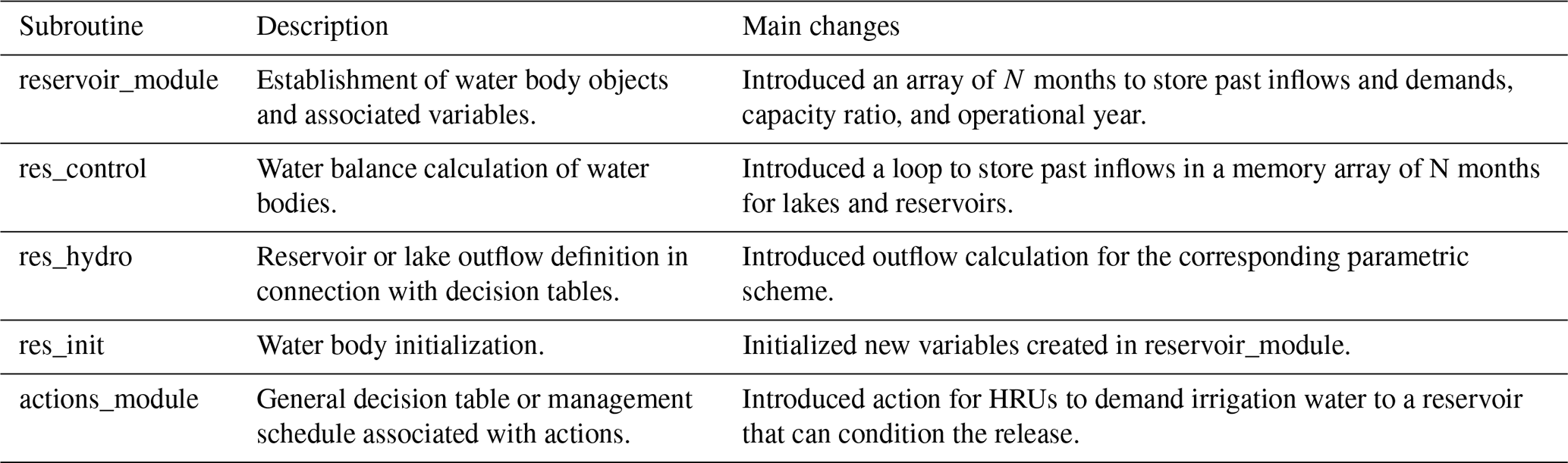
B1 Additional figures

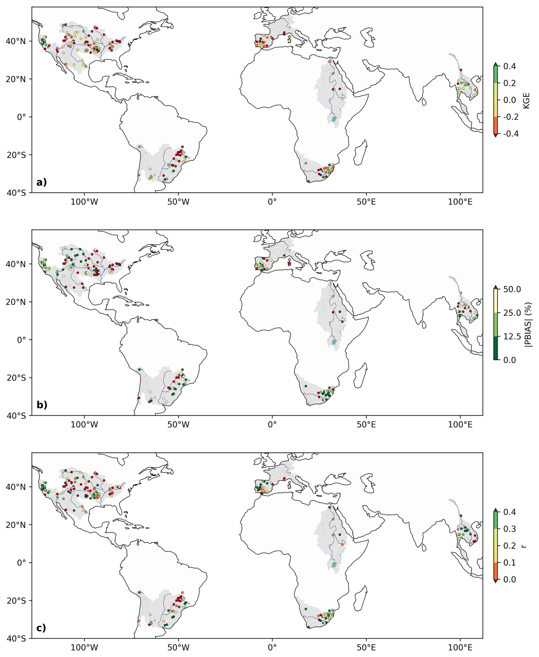
Figure B1 Spatial distribution of model performance statistics. (a) KGE, (b) |PBIAS|, and (c) coefficient of correlation (r) for reservoir storage.

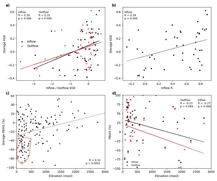
Figure B2 Scatter plots showing relationships between reservoir performance metrics, inflow characteristics, and elevation. Panels (a) and (b) include only reservoirs with monthly storage KGE greater than −0.42, comparing monthly storage KGE with (a) monthly inflow.

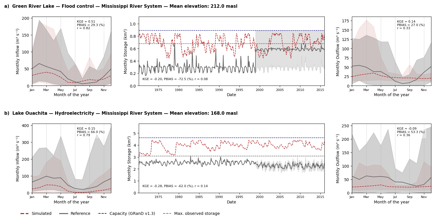
Figure B3 Monthly inflow climatology (left panels), storage (center panels), and outflow climatology (right panels) for two reservoirs where storage performance was significantly degraded by an initial storage condition set above actual operational levels. Reference observations also show high variability across datasets. Shaded areas in climatology plots represent ±1.5  SD (standard deviations); shaded areas in storage panels indicate the range between maximum and minimum reported values across datasets.

B2 KGE skill score to identify significantly influenced streamflow stations

The change in performance by new implementations was then quantified using the KGE skill score (Towner et al., 2019):

$$\begin{array}{}\text{(B1)}& {\mathrm{KGE}}_{\mathrm{SS}}={\displaystyle \frac{{\mathrm{KGE}}_{\mathrm{with}}-{\mathrm{KGE}}_{\mathrm{without}}}{\mathrm{1}-{\mathrm{KGE}}_{\mathrm{without}}}}\end{array}$$

where KGE_with and KGE_without denote the model performance with and without the new implementations, respectively. The KGE skill score was used mainly as a filtering criterion to distinguish meaningful changes in performance: stations where $\left|{\mathrm{KGE}}_{\mathrm{SS}}\right|$ were below 0.05 and were considered not to exhibit significant changes and were therefore excluded from further analysis.