A data-driven method for identifying climate drivers of agricultural yield failure from daily weather data

Climate-related impacts, such as agricultural yield failure, often occur in response to a range of specific weather conditions taking place across different time periods, such as during the growing season. Identifying which weather conditions and timings are most strongly associated with a certain impact is difficult because of the overwhelming number of possible predictor combinations from different aggregation periods. Here we address this challenge and introduce a method for identifying a small number of climate drivers of an impact from high-resolution meteorological data. Based on the principle that causal drivers should generalize across different environments, our proposed two-stage approach systematically generates, tests, and discards candidate features using machine learning and then generates a set of robust drivers. We evaluate the method using simulated US maize yield data from two process-based global gridded crop models and rigorous out-of-sample testing (using approximately 30 years of early 20th-century climate and yield data for training and over 70 years of subsequent data for testing, as well as a held-out spatial and spatiotemporal test set). The climate drivers identified align with crop model mechanisms and consistently use only the weather variables that are taken as input by the respective models. Logistic regression models using ten drivers as predictors show strong predictive performance on the held-out test period even under shifting climatic conditions, achieving correlations of 0.75–0.91 between predicted and true annual proportions of grid cells experiencing yield failure. This approach circumvents the limitations of post-hoc interpretability in black-box machine learning models, allowing researchers to use parsimonious statistical models to explore relationships between climate and impacts, while still harnessing the predictive power of high-resolution, multivariate weather data. We demonstrate this method in the context of agricultural yield failure, but it is also applicable for studying other climate-related impacts such as forest die-off, wildfires, landslides, or flooding.

1 Introduction

Climate impacts to human and natural systems are often highly dependent on the weather conditions experienced during specific time periods. For instance, annual crop yields are most influenced by the climatic conditions during the growing season, and may be more sensitive to certain weather conditions at different growth stages. For maize, up to 60 % of the variance in US yields at national or county level has been explained by climate variables (Frieler et al., 2017; Mistry et al., 2017), and process-based crop models, which encapsulate the day-by-day biophysical plant response to weather conditions, have been able to explain up to 79 % of US maize yield variation (Müller et al., 2017). However, current models have been found to exhibit very different responses to climate drivers (Müller et al., 2024) and vary widely in their projections of climate change impacts (Jägermeyr et al., 2021; Wang et al., 2024). Crop models generally include heat and drought stress effects, as well as other temperature and moisture responses, but have been shown to underestimate the impact of such extremes (Heinicke et al., 2022). Researchers have argued that models do not consider the influence of compound stressors on yields due to knowledge gaps (Webber et al., 2022), and that improved scientific understanding of these relationships is needed to inform and constrain the next generation of crop models (Kim et al., 2025; Nóia Júnior et al., 2025).

The impacts of weather on agricultural yields are complex and nonlinear (Siebert et al., 2017a). High temperatures during growing seasons in the US have been consistently linked with negative maize yield effects (Schlenker and Roberts, 2009; Schauberger et al., 2017; Zhao et al., 2017), but the impact is reduced by irrigation (Troy et al., 2015; Siebert et al., 2017b) and can be mitigated or exacerbated by the co-occurring level of precipitation, soil moisture or evapotranspiration (Lobell et al., 2013; Jin et al., 2017; Matiu et al., 2017; Mistry et al., 2017; Rigden et al., 2020; Haqiqi et al., 2021; Lesk et al., 2021; Ting et al., 2023). Additionally, as plant phenology develops, their sensitivity to weather conditions changes. For example, the effect of short-term heatwaves on yields is more severe during the reproductive or grain-filling period of maize development than the vegetative period (Siebers et al., 2017; Zhu et al., 2019).

Machine learning (ML) models, which can capture highly complex and nonlinear relationships and are well-suited for high-dimensional tasks, are also being explored for agricultural yield forecasting and modelling (Sweet et al., 2025). A wide range of approaches have been able to predict US maize yields with good performance (Crane-Droesch, 2018; Martínez-Ferrer et al., 2020; Lin et al., 2020; Liu et al., 2022). However, just like statistical models, ML models are vulnerable to confounding effects, and their increased flexibility allows them to more easily overfit to spatiotemporal dependencies. This leads to poor predictive performance in years or regions outside of the training data (Ferraciolli et al., 2019; Shahhosseini et al., 2019; Silva et al., 2023; Sweet et al., 2023; Filippi et al., 2024), suggesting that the relationships learned by the models are not robust, and therefore unlikely to reflect the underlying physical processes. “Knowledge-guided” or “hybrid” ML, in which known process understanding is embedded into the model structure or training procedure, can help ameliorate this, but can also potentially degrade model performance if the constraints used are not well-specified (Moon et al., 2023; Han et al., 2025). “Post hoc” interpretable or explainable techniques, in which the structure of a trained model or its response to interventions on input variables is analysed, have also been used to study the relationships learned by complex ML models and thereby improve process understanding (Shahhosseini et al., 2019; Hoffman et al., 2020; Ryo, 2022; Jiang et al., 2024a, b). However, in studies employing ML to analyse relationships between climate and impacts, variables are used, in general, if it is plausible that they could play a causal role. This means that spurious relationships learned by the model, or inaccurate interpretations, are difficult to detect. This could be a substantial issue given that studies have shown commonly-used methodologies to give contradictory results (Lischeid et al., 2022; Mamalakis et al., 2022), return spurious or physically-implausible relationships (Wadoux et al., 2020; Sweet et al., 2023), or even fail to out-perform random guessing (Bilodeau et al., 2024).

Statistical models, on the other hand, are often inherently interpretable, and have been frequently used to study the relationships between weather and crop yield (Vogel et al., 2019, 2021; Heilemann et al., 2024). Before fitting these models, a parsimonious set of predictive variables must be chosen, which can significantly impact model behaviour (Chen et al., 2024). In most studies that aim to predict climate-related yield variability, climate conditions are approximated by the annual or growing-season mean precipitation or temperature, or by indicators selected based on expert knowledge, such as the number of growing-degree days or extreme degree days, the maximum or minimum temperature experienced, and the average diurnal range. However, this can obscure relationships that are not captured by the chosen aggregate variables, such as the effect of short-term weather events at different phenological stages. Selecting a parsimonious set of features that reflect the underlying biophysical relationships requires a high level of domain expertise, and does not allow for the discovery of unexpected or more specific climate drivers.

We propose a data-driven method for obtaining simple, human-understandable climate drivers of yield failure, inspired by the idea that causal drivers should generalise to unseen environments (Peters et al., 2016; Richens and Everitt, 2024). This allows researchers to use parsimonious, interpretable models to explore relationships between weather and impact, while still making use of the information available in high-dimensional, multivariate climate data, rather than using non-robust post hoc interpretation methods to approximate the functionality of trained black-box ML models. To validate the method’s performance and robustness, we make use of simulated US maize yields from global gridded process-based crop models (pDSSAT and LPJmL). This allows us to compare the identified drivers to known model mechanisms, and to test the predictive skill of models using these drivers under conditions that reflect the challenges inherent to observational studies, such as correlation between predictive variables, sampling bias from the increased availability of data in locations where climate conditions favour higher yields, and distribution shifts induced by the changing climate. Our testbed consists of simulations driven by climate reanalysis spanning 1902–2016, but we use only the first 30 % of the timeseries to identify drivers and train models and then test their performance over the last 70 %. This train-test split is more rigorous than in most ML studies and allows us to examine the suitability of the method for conducting similar analyses using observational data under the influence of climate change. We also examine the skill of models when applied to unseen spatial regions by splitting the dataset by latitude, using data from latitudes above 35° for identifying drivers and training models and then testing model performance on lower latitudes. We then demonstrate the application of the method to county-level reported US maize yield and observed meteorological data.

2 Data

We use gridded simulations of US rainfed maize yield from two process-based crop models: LPJmL (von Bloh et al., 2018; Lutz et al., 2019) and pDSSAT (Jägermeyr et al., 2021). LPJmL is a dynamic global vegetation model, designed to capture terrestrial carbon and water cycles of natural and agricultural systems. pDSSAT (Jones et al., 2003; Elliott et al., 2014), on the other hand, has been developed to simulate field-scale processes, with a focus on the interactions between crop development, soil, atmosphere and management factors.

Both crop models were driven by daily climate data spanning 1901–2019, at 0.5° spatial resolution, based on reanalysis from W5E5 v2.0 (Cucchi et al., 2020; Lange et al., 2021) and GSWP3 v1.09 (Dirmeyer et al., 2006; Kim, 2017). The data was homogenised to W5E5 for 1901–1978 using the ISIMIP3BASD v2.5.0 bias adjustment method (Lange, 2019, 2021). The simulations were produced according to the ISIMIP3a protocol and all forcing data, as well as the corresponding simulated yields, are publicly available from the ISIMIP data repository (Lange et al., 2022). Sowing dates are based on a combination of observational data products (Jägermeyr et al., 2021) and vary spatially but not year-to-year. The models were also given annual atmospheric CO₂ concentrations and soil parameters, which we do not consider for this study. We restrict our study area to current maize cropping areas of the continental US, which we define as grid cells containing at least ten harvested hectares according to the MIRCA2000 data product (Portmann et al., 2010).

We use all ten climate variables provided to impact models in the ISIMIP simulation protocol at daily resolution: near-surface relative humidity (hurs, %), near-surface specific humidity (huss, kg kg⁻¹), precipitation (pr, mm), surface air pressure (ps, Pa), surface downwelling longwave radiation (rlds, W m⁻²) and shortwave radiation (rsds, W m⁻²), near-surface windspeed (sfcwind, m s⁻¹), near-surface air temperature (tas, °C), daily minimum (tasmin, °C) and maximum near-surface air temperature (tasmax, °C). However, each crop model only considers a subset of those variables; both models take pr, tasmin, tasmax, rsds, and rlds as input, and LPJmL additionally uses sfcwind and tas. pDSSAT does not use tas, but internally estimates hourly temperatures based on daily tasmin and tasmax values.

Annual county-level observed maize yields are obtained from the United States Department of Agriculture National Agricultural Statistics Service (USDA NASS) for 1983–2018 (United States Department of Agriculture (USDA), 2025), and county-level boundaries are obtained from the US Census Bureau’s 2018 TIGER/Line shapefiles (U.S. Census Bureau, 2018). Yields are detrended by subtracting a five-year rolling mean, and counties are removed from the dataset if, after detrending, fewer than ten years of yield data are available. We limit the dataset to counties in which maize harvested areas are predominantly rainfed and at least 100 ha are harvested (according to MIRCA2000), resulting in 551 total counties. In the majority of counties, yields are not reported separately for rainfed or irrigated areas. For counties in which yields are reported separately, rainfed yields are used only if available for all years. Otherwise, and for all other counties, overall reported yields are used.

Observed daily meteorological data over the same time period, at 4 km spatial resolution, is obtained from the PRISM climate group (PRISM Group, 2018). This dataset has been used in a number of previous studies analysing the climate drivers of agricultural yields in the US (Roberts et al., 2013; Ortiz-Bobea et al., 2019; Hogan and Schlenker, 2024). The variables are aggregated to county-level using a weighted average of overlapping grid cells based on enclosed cropping area. Variables used consist of daily minimum and maximum temperature (°C), minimum and maximum vapour pressure deficit (hPa), precipitation (mm) and dewpoint temperature (°C). Daily mean temperature and vapour pressure deficit is estimated by averaging the minimum and maximum values, resulting in a total of eight meteorological variables.

3 Methods

3.1 Setup

Each datapoint in our compiled dataset consists of a binary target variable and the corresponding daily multivariate climate input for one growing season at one grid cell. Due to the trends in yields due to improved management practices and breeding that have occurred over the last decades, researchers often consider yield anomalies (after detrending) rather than their absolute values. We test our method on both non-detrended and detrended yields (based on subtracting a seven-year rolling mean, meaning that we discard datapoints from the first six years), in order to assess the utility of the method for analysis of both relative yield failure and the occurrence of yields below an absolute threshold. The target variable is maize yield failure, which we define as any yield below the 10th percentile observed during the training period at that grid cell. We assess the robustness of our method to this choice by reproducing the results using 5th and 15th percentile thresholds. The dataset is split into a training set (the first 30 % of growing seasons, covering 1902–1937 for non-detrended yields and 1907–1940 for detrended, and all grid cells with latitudes above 35° north) and three test sets: a temporal test set (the last 70 % of growing seasons, covering 1938–2016 and 1941–2016, for grid cells of latitude above 35°), a spatial test set (the first 30 % of growing seasons in grid cells below 35°) and a spatiotemporal test set (the last 70 % of growing seasons in grid cells below 35°). Note that, for non-detrended LPJmL yields, the 10th percentile over the training years was zero for 167 grid cells. These low-yielding areas are removed from the training and test set. After processing, the training sets are made up of 50 000–60 000 datapoints, the temporal test sets consist of 115 000–135 000, the spatial test sets 13 000–18 000, and the spatiotemporal test sets 30 000–39 000.

Our predictive variables derive from the same daily multivariate climate data that was used to drive the crop models. For each grid cell and year, we take 90 days (d) of each climate variable before the planting date (to consider e.g. lagged soil moisture effects) and 240 d after, resulting in a 3300-dimensional dataset (as we have ten climate variables). To use an interpretable model with this data, a smaller number of climate drivers must first be defined (generally, by applying aggregation functions over specified time intervals – for instance, the monthly maximum temperatures or number of growing degree days during the growing season). This feature selection step is normally based on expert knowledge. Instead, our proposed method extracts a small number of simple climate drivers of yield failure from daily multivariate weather data based on their robust predictive power in held-out time periods.

3.2 Approach

The method for identifying climate drivers consists of three steps (Fig. 1): first, we generate 100 pools of candidate features by using a set of chosen aggregations (mean, minimum, maximum, number of days below 0, number of days above the 90th percentile, minimum and maximum 5 d mean) over each daily climate variable from 30 randomly-sampled time intervals (with minimum duration of two weeks) during the growing season; second, we select ten features from each pool using sequential forward feature selection, based on the predictive performance of ML models on held-out time periods; finally, we collect the selected features from the pools, and extract a set of ten condensed climate drivers from that collection using agglomerative clustering, based on the aggregation methods, variables and periods of the growing season which are selected most frequently.

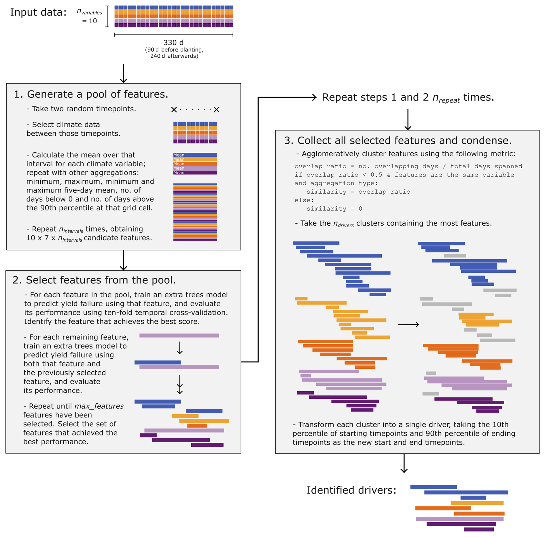
Figure 1 Flowchart illustrating our proposed method to identify a small number of simple climate drivers from multivariate time series weather data. The method requires some parameters to be chosen: n_intervals, the number of random time intervals to sample for each pool of candidate features; max_features, the maximum number of features to select from each pool and n_drivers, the number of condensed drivers desired. Additionally, the cross-validation strategy used when selecting features from each pool must be specified.

When selecting features from each pool (step 2), we use an extremely randomised trees model (extra trees). This model consists of an ensemble of decision trees, similar to the more widely-known random forest, but rather than identifying the optimal split value for each feature at each node, the thresholds are selected at random. Extra trees models are therefore faster to train, and can result in smoother functional relationships when predictions are averaged across trees, leading to improved out-of-sample performance (Geurts et al., 2006). Like other tree-based models, they handle nonlinear relationships well, are robust to outliers and skewed distributions, are computationally efficient, and can be trained in parallel. We do not tune hyperparameters; all models used consist of 50 trees of maximum depth 30. At each split, half of the predictive variables are considered, and each leaf node must contain a minimum weighted fraction of 0.0001 of all samples (with samples weighted inversely proportionally to class frequency). Features are selected sequentially based on optimising model performance using ten-fold temporal cross-validation, with each test fold consisting of a held-out period of three or four consecutive years.

To obtain a final set of ten climate drivers of yield failure we apply agglomerative clustering to the selected features from 100 pools of candidates (step 3). Features are only clustered together if they substantially overlap in time and use the same aggregation method and climate variable. The ten largest clusters are then condensed into single drivers by using the 10th percentile of starting timepoints and 90th percentile of ending timepoints within the cluster as the new start and end timepoints. To create simple and interpretable models, we then fit logistic regression models using the ten identified drivers. Climate drivers are identified and models are trained using the training data only. We perform this procedure (identify ten features, fit logistic regression model) for both crop models.

3.3 Model evaluation and sensitivity analyses

We evaluate model performance and the robustness of our approach to different parameter choices in several ways. The ability of the final logistic regression models to predict yield failure over the three held-out test sets is assessed using four performance metrics: (i) the area under the receiver operating characteristic curve (ROC AUC), a ranking metric that reflects the ability of the model to distinguish between binary classes at a range of classification thresholds; (ii) the average precision, which measures the tradeoff between precision and recall at different classification thresholds; (iii) the Brier score loss, which measures the mean squared difference between each predicted probability and the true (binary) outcome; (iv) and the logistic loss (log loss), also known as the cross-entropy loss, which measures the negative log-likelihood of each predicted probability given the true outcome. Note that the prediction task is an imbalanced classification problem, with non-failure years occurring approximately nine times as frequently as yield-failure years. Additionally, we investigate the ability of the model to capture temporal patterns in yield failures over both the training and held-out region by calculating the percentage of grid cells each year predicted to be experiencing yield failure and comparing this to the simulated “ground truth”. As predictions from the logistic regression model range between 0 and 1, we select a threshold to define yield failure that achieves the maximal f-score (the harmonic mean of the precision and recall) over the training set.

We assess if drivers are plausible by checking whether they only include the variables used as input by the crop models (i.e., ps, hurs and huss should not appear, nor should sfcwind for pDSSAT). We also compare their distributions between yield failure and non-yield failure years and assess their consistency with associations captured by interpretable models and expert judgement.

We further test the robustness of the approach by conducting 100 bootstrap repeats, sampling 20 pools (with replacement) from the 100 pools described above. For each repeat, we extract sets of ten climate drivers from the 20 pools, and evaluate the extent to which these sets consist of the variables actually taken as input by the crop models by counting the variables used by the features collected from each pool (in Step 2 of the driver identification method), and from the condensed drivers over all bootstrap repeats. Second, for each of the repeats, we construct models with 5, 10 or 15 identified drivers and evaluate their predictive performance over the three test sets, in comparison to a variety of commonly-used baseline feature sets. An assessment of model performance estimates using up to 1000 bootstrap repeats, for Lasso logistic regression models on the temporal test set for LPJmL, suggests that 100 repetitions is sufficient for stable model performance estimation (Fig. A1).

The baseline feature sets consist of mean climate conditions aggregated over different time intervals: either the growing-season (defined as 180 d after planting), or on a quarterly (three consecutive ninety-day intervals after planting) or monthly (six consecutive thirty-day intervals after planting) basis. These are calculated for a subset of the climate variables (pr, tas and rsds) or for all ten. In addition, we include five extreme indicators that are often used in data-driven agricultural yield models (Vogel et al., 2019, 2021). These are calculated over the first 180 d after planting, and consist of the minimum and maximum temperatures experienced, the maximum five-day precipitation sum, the number of days in which the temperature drops below 0 °C, and the number of days in which temperatures exceed the 90th percentile (as defined during the training period for each grid cell). This results in six baseline feature sets containing between 8 and 65 weather features.

As the number of predictors can affect model performance, to facilitate a fair comparison between the baselines and the sets of climate drivers identified using our approach, we use Lasso logistic regression models, which uses L1 regularisation to force the coefficients of less important features to 0, effectively performing feature selection. Predictors are first scaled by removing the median and scaling to the 10th and 90th quantile range (based on training-set statistics), and the value of the hyperparameter α, which controls the level of regularization, is selected using five-fold temporal cross-validation over the training years and regions. We also compare results when including second-order interaction terms and when using more complex extra trees models (with the same hyperparameters as previously described).

Finally, we assess the robustness of the approach to a number of parameter and methodology choices. For these sensitivity tests, performance is measured using a temporal train-test split, with drivers identified and models trained on the first 30 % of growing seasons and tested on the final 70 %. The cross-validation strategy chosen when selecting features from each pool is important (Sweet et al., 2023; Meyer et al., 2019, 2018). We explore the impact this choice has on the results by comparing model performance scores when using three other cross-validation strategies (random sampling, spatial clusters and clusters in feature-space) in addition to the temporal strategy described above. We also test the impact of using 5, 10 or 15 cross-validation folds. Furthermore, we conduct sensitivity tests in which several parameters of our method are varied both individually and in combination: the number of time intervals sampled in each pool of candidate features, the maximum number of features selected from each pool, and the number of drivers identified.

3.4 Demonstration on observational data

Observational data is split into training years (1983–2007) and test years (2008–2017). County-level yield failure years are determined based on falling below the tenth percentile of (detrended) yields over the training period. Using maize planting dates from WorldCereal (Franch et al., 2022), daily multivariate climate data is obtained for 90 d before planting and 240 subsequent for each year and county.

After processing, the method is applied on the training data to obtain four climate drivers in the same manner as described above. 100 pools of candidate features are obtained based on 20 sampled time intervals per pool, and ten features are selected from each using five-fold temporal cross-validation and extra trees models. The obtained drivers are then used to fit a logistic regression model to the training data, and performance is evaluated on data from the test years.

4 Results

4.1 Crop model simulations

Maize yields simulated by pDSSAT are more variable in space and time than LPJmL, but both simulations exhibit lower average yields in the western regions of the US and declining annual yields until the late 1930s, followed by an upward trend (Fig. 2a–c). As management and genetic changes over time are not considered in these simulations, this behaviour is the result of changing climate conditions, and in fact these trends coincide with opposing shifts in average growing-season temperatures (Fig. 2d). The high spatial variability in simulated yields and temperatures suggests that a space-for-time substitution may be able to improve the ability of data-driven models to extrapolate to warmer (future) years. Despite increasing temperatures in later decades, most locations experiencing an unprecedentedly-warm growing season are unlikely to be outside of the range of previously-experienced conditions at all grid cells until that year.

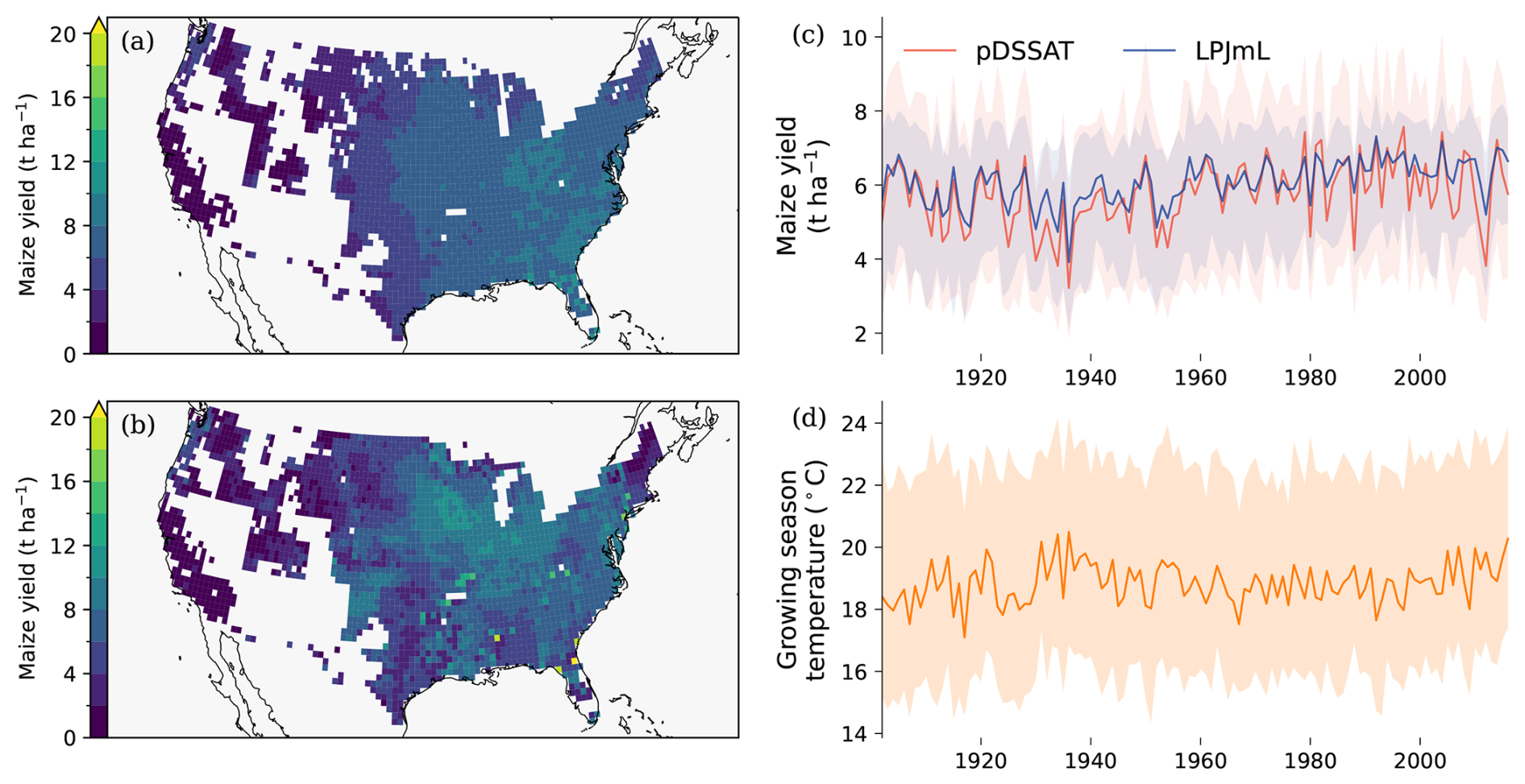
Figure 2 Overview of the rainfed maize yield simulations from both crop models. (a, b) Average yields over the entire time period studied, for LPJmL and pDSSAT respectively, for grid cells included in the dataset. (c) Distributions of yields from year to year, with darker lines denoting the median yield across all grid cells for each crop model, and shaded regions covering the interquartile ranges. (d) Distribution of annual growing season temperatures (here defined as the average daily mean temperature in the first 180 d after planting) in the corresponding climate forcing data.

Composite plots of the growing-season daily climate conditions for normal and yield-failure years suggest that non-causal climate variables are associated with yield failure in these simulations for both crop models (Fig. 3, with further variables in Fig. A2). For example, near-surface relative humidity is not used as input for LPJmL or pDSSAT, but yield failure years tend to have drier growing seasons in both crop models (Fig. 3g and h). Composite plots of growing-season windspeed show an association between lower winds and yield failure for both models (Fig. A2i and j), despite the fact that windspeed is an input variable for LPJmL but not pDSSAT. Yield-failure years tend to have higher growing-season temperatures, but there is a wide overlap in temperature conditions between failure and non-failure years (Fig. 3c and d). Similarly, periods of low rainfall in the first four months after sowing are associated with yield failure, but many non-failure years also experience periods of low rainfall at that time (Fig. 3e and f). Furthermore, while simulations from the two crop models differ in the proportion of grid cells experiencing yield failure by up to 10 % in some years (Fig. 3a and b), relationships suggested by all composite plots are visually similar. Composite plots of growing-season daily climate conditions for normal and yield-failure years when yields are detrended are very similar (Figs. B1 and B2).

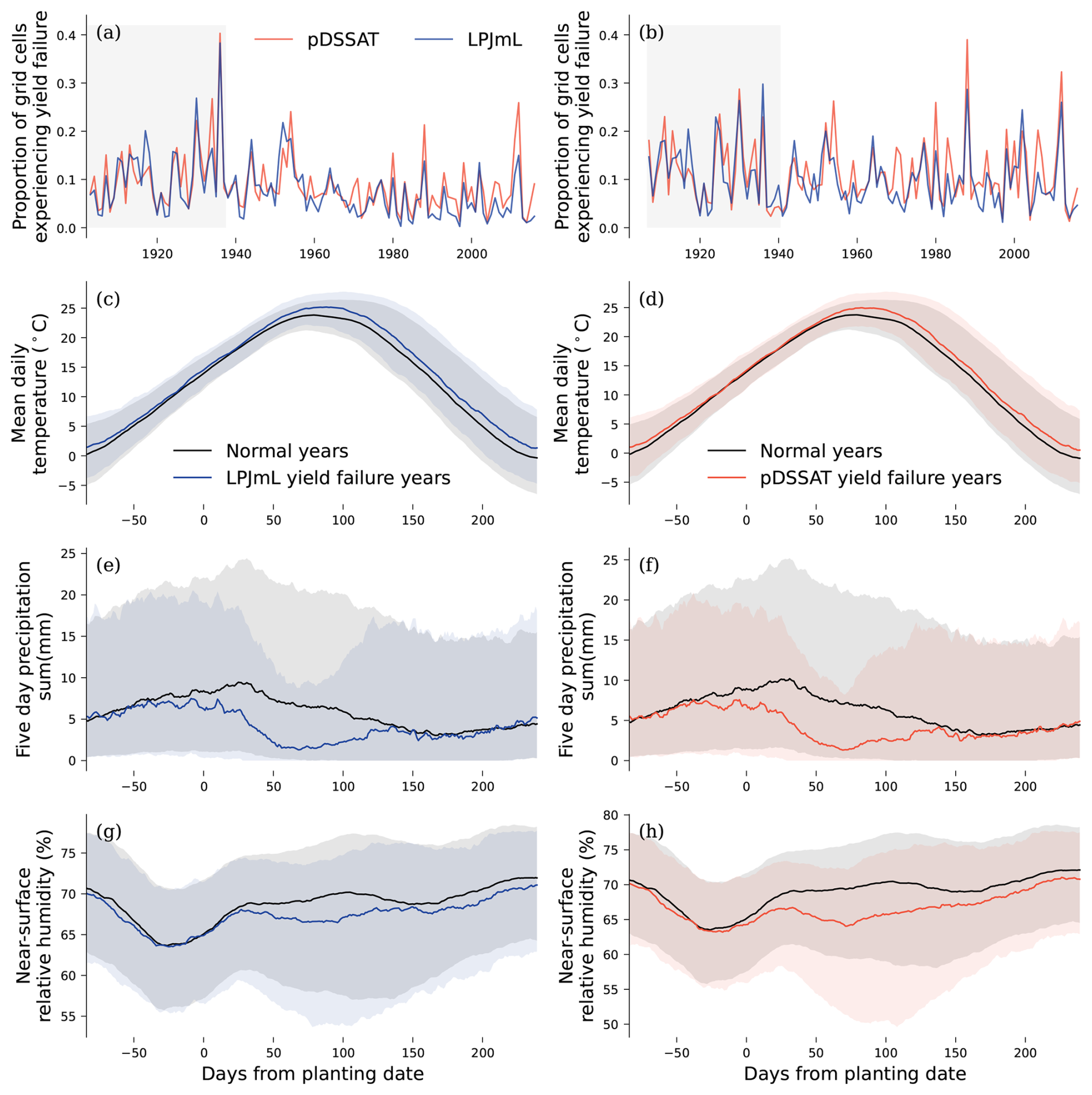
Figure 3 (a) Proportion of grid cells experiencing yield failure for each year of the studied period. Pale grey shaded years denote the training period used for identifying drivers and training predictive models. All other years are held out and used to evaluate model performance. (b) Same as (a) after yields are detrended based on subtracting the seven-year rolling average. (c–h) Composite plots of mean daily temperature, five day precipitation sums and near-surface humidity ((c, e, g) for LPJmL and (d, f, h) for pDSSAT). Solid lines denote the median daily climate conditions over all datapoints (year and gridcell combinations) where yield failure did not occur (grey) or all datapoints where yield failure did occur (blue/red), and shaded regions indicate the interquartile range. Mean daily temperature and near-surface relative humidity are smoothed by taking the seven-day rolling mean.

4.2 Resulting interpretable models perform well on held-out years and regions

A logistic regression model fit on the training data using ten identified climate drivers of pDSSAT yield failure as predictors is able to achieve a ROC AUC of 0.83, average precision of 0.32, Brier score of 0.056 and log loss of 0.20 on the held-out test years. Comparable scores are achieved when applied to the held-out spatial test set (covering the same growing seasons as used for identifying drivers and training the model) and the spatiotemporal test set (including only held-out years and locations) (Table 1). Notably, the model is able to outperform lasso logistic regression models using all baseline climate feature sets tested for all metrics calculated and for all held-out sets. The model captures the year-to-year variability in yield failure well (Fig. 4a), with a Pearson correlation of 0.84 between the true and predicted annual proportions of grid cells experiencing yield failure over the training region (above 35° latitude) and 0.91 over the held-out region (below 35° latitude). Notably, model performance does not appear to deteriorate over time: annual ROC AUC scores slightly increase over the decades, while Brier score and log loss decrease. Maps of predictions and ground truth in 2011, in which the majority of grid cells in the lower latitudes experienced a yield failure (Fig. 4c and d) show general agreement in spatial variability, including over the held-out lower latitudes in which yields were most adversely impacted.

Table 1 Performance scores achieved by a logistic regression model with ten identified climate drivers as predictive variables on the three different test sets, for non-detrended data. The best performance for each metric and test set achieved by any of the baseline climate feature sets (annual, three-month or monthly averages of either all ten climate variables or a subset of three: precipitation, mean daily temperature and short-wave radiation; with and without extreme indicators) using a lasso logistic regression model, using 5-fold temporal CV to select the value of alpha, is reported in brackets and in italics for comparison. Scores in bold are the best achieved.

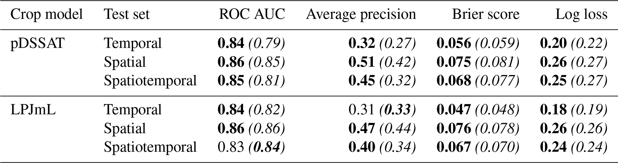
A logistic regression model using ten climate drivers for LPJmL is able to achieve similarly high performance (Table 1, Fig. A3). A Pearson correlation of 0.76 is achieved between true and predicted annual proportions of grid cells experiencing yield failure in the training regions and 0.87 in the held-out lower latitudes. Similar levels of model performance are achieved for both crop models when yields are detrended before defining yield failure (Figs. B3 and B4).

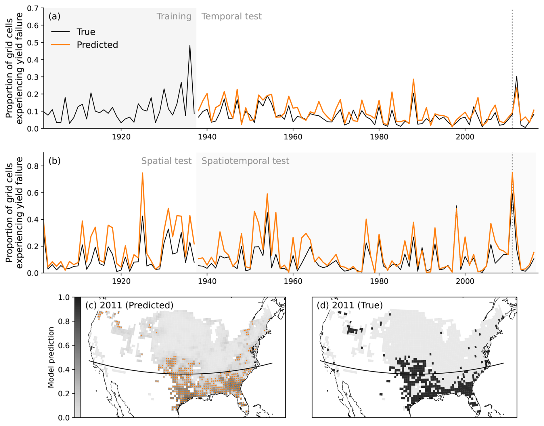
Figure 4 Predictions of a logistic regression model using ten identified pDSSAT drivers on held-out years and regions. (a) True (black) and predicted (orange) proportion of grid cells experiencing yield failure each year over the grid cells used for training (latitudes above 35°), using a threshold of 0.235 to define a yield failure prediction (selected based on achieving the maximal f-score of 0.405 over the training years, which are marked by the grey shaded area). (b) True (black) and predicted (orange) proportion of grid cells experiencing yield failure each year in the held-out grid cells (latitude below 35°). Unshaded years represent the spatial test set (held-out regions during years included in training data) and shaded years represent the spatiotemporal set (held-out regions and years). Model predictions for 2011 are illustrated in panel (c), with orange dots marking grid cells where the prediction exceeds the threshold and therefore yield failure is predicted. The corresponding ground truth is shown in panel (d), with black areas indicating locations experiencing yield failure. The curved line indicates the spatial split used to define the test sets. No data from locations below the line, from any year, is used for identifying drivers or training the model.

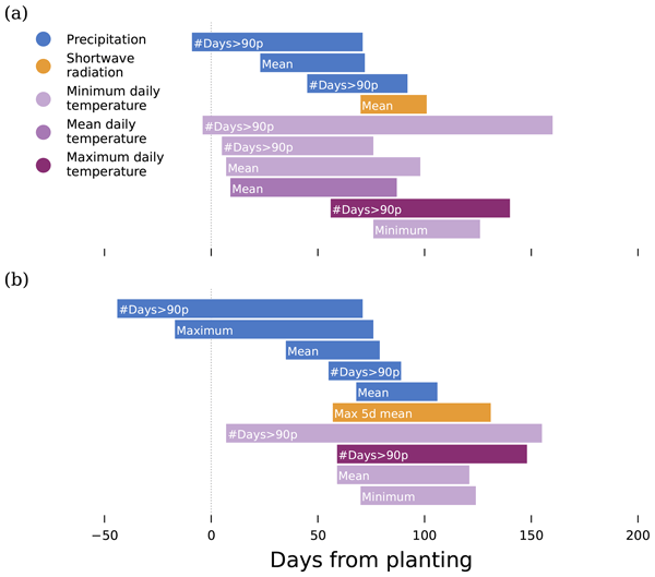
The ten climate drivers of yield failure identified by our method for each crop model consist of variables that are taken as input by those respective models, with the exception of one driver based on mean daily temperature for pDSSAT (Fig. 5). However, as pDSSAT takes as input the daily minimum and maximum temperatures and uses them to estimate hourly average temperatures for use in model processes, it could be argued that mean daily temperature is a plausible driver. For both crop models, several drivers are aggregates of daily precipitation and, in combination, span a time period starting before planting and ending four months afterwards, with overlap between drivers. In terms of aggregation methods selected, precipitation drivers identified measure the number of days above the 90th percentile, which can be interpreted as the number of rainy days, the maximum daily precipitation, or the mean daily precipitation over a time interval, which would be proportional to the cumulative rainfall in that period.

Temperature is strongly represented in climate drivers for both crop models, but temperatures earlier in the growing season are more often identified for pDSSAT (four drivers) than LPJmL (one driver). Three of the temperature drivers are almost identical across both models: the number of days of minimum daily temperatures above the 90th percentile from around planting date up until around five months afterwards; the number of days of maximum daily temperatures above the 90th percentile over a three-month period starting around two months after planting; and the minimum temperature experienced over a two-month period starting around ten weeks from planting. Shortwave radiation is included in the set of drivers for both crop models. No identified drivers take into account the climate conditions later than six months from planting, and the only variable considered before planting is precipitation.

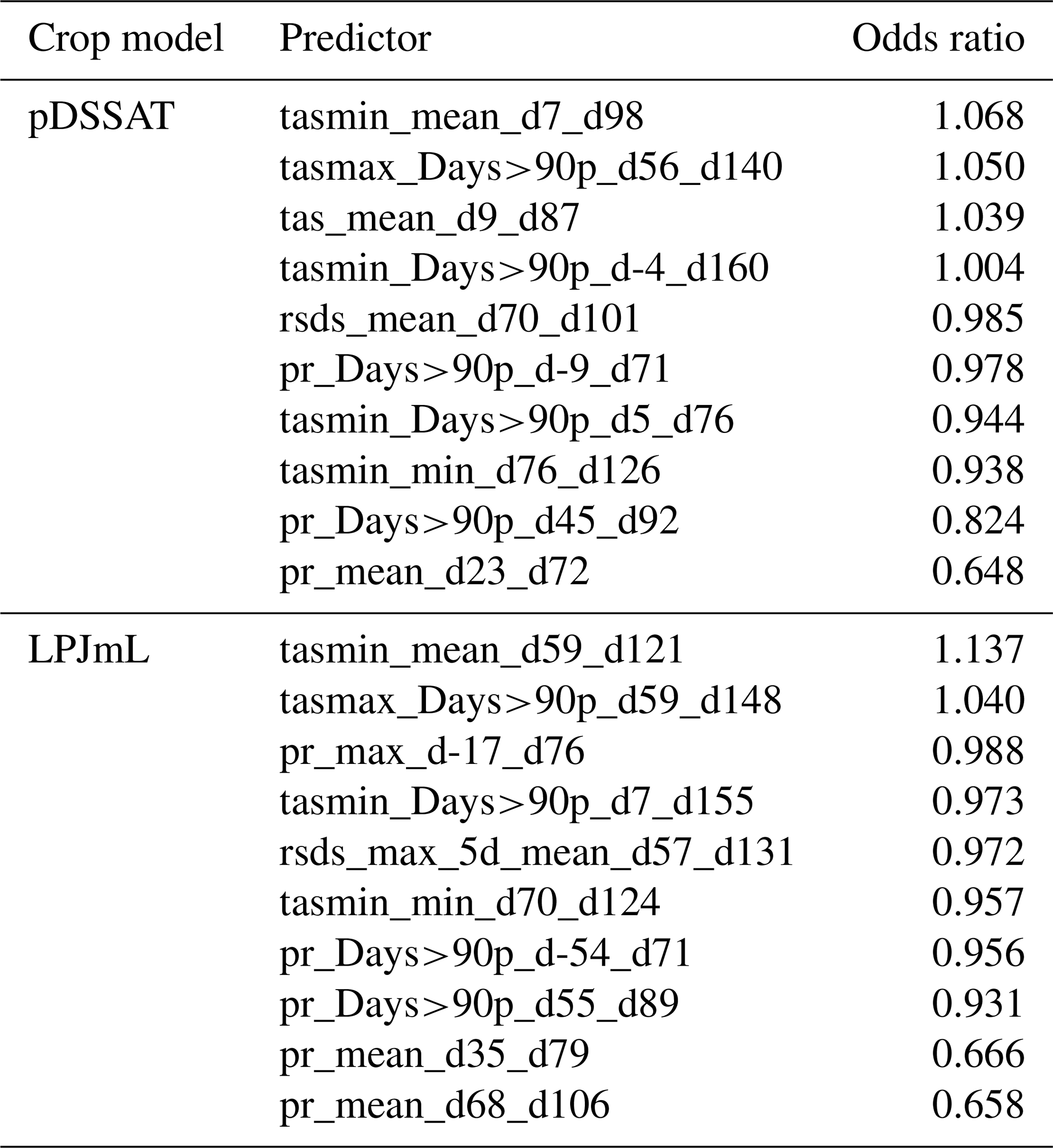
Analysis of the relationships between identified climate drivers and yield failure is made possible by the use of simple, interpretable models. Odds ratios associated with the climate drivers for fitted logistic regression models are reported in Table 2. Odds ratios greater (smaller) than one indicate higher (lower) odds of yield failure given a one-unit increase in the predictor, conditional on the other predictors of the model, while an odds ratio equal to one would suggest no association of that predictor with yield failure, in this model. For both crop models, climate drivers are based on mean precipitation are highly influential, with increased rainfall strongly associated with lower yield failure probability. Additionally, the climate drivers with the strongest positive association with yield failure are temperature-related. For both crop models, however, both positive and negative associations with yield failure are identified for temperature-related drivers, pointing towards nonlinear relationships between growing-season temperature and yield failure probability.

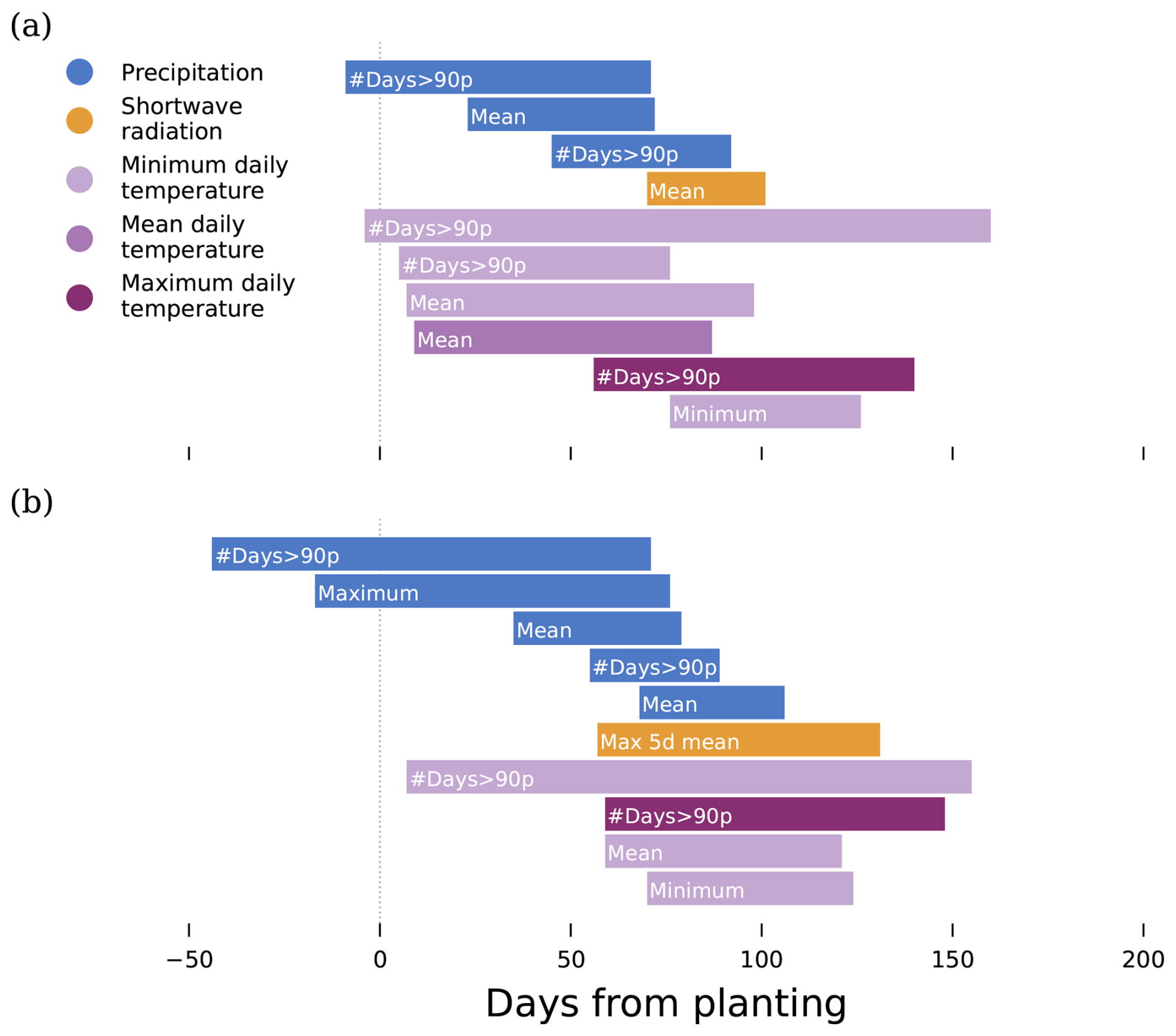
Figure 5 Identified climate drivers of maize yield failure for (a) pDSSAT and (b) LPJmL, based on using 30 sampled time periods to generate 100 pools of candidate features, using ten-fold temporal cross-validation to select ten features from each pool, and condensing the resulting 1000 features to ten drivers. Each climate driver is denoted by a coloured horizontal bar, and consists of an aggregated daily climate variable over a time interval which is defined relative to the planting date (illustrated by the bar’s length and position). The caption overlaid on each bar describes the aggregation method used (i.e., “mean” indicates that the corresponding daily climate values are averaged over the time period selected; “#Days>90p” means the number of days in which the respective variable exceeds the 90th percentile for that location; “Max 5d mean” takes the maximum value of the five-day rolling mean of the respective climate variable over the selected time period). Drivers are ordered by variable and start date.

Table 2 Odds ratios of maize yield failure associated with a unit increase in each predictor, based on the coefficients of logistic regression models fit using 10 identified climate drivers for pDSSAT and LPJmL. Predictors are labelled with the climate variable used, the aggregation method, and the beginning and end day (in relation to the planting date) of the time interval over which the aggregation is applied. Predictors are sorted by magnitude of the odds ratio.

When yields are detrended before applying the method, the precipitation- and temperature-related drivers identified are largely similar to those identified without detrending for both crop models (Fig. B5). Climate conditions later than six months after planting are again not considered. However, when yields are detrended, short-wave radiation is not used by any of the climate drivers identified for pDSSAT, and one of the drivers uses specific humidity.

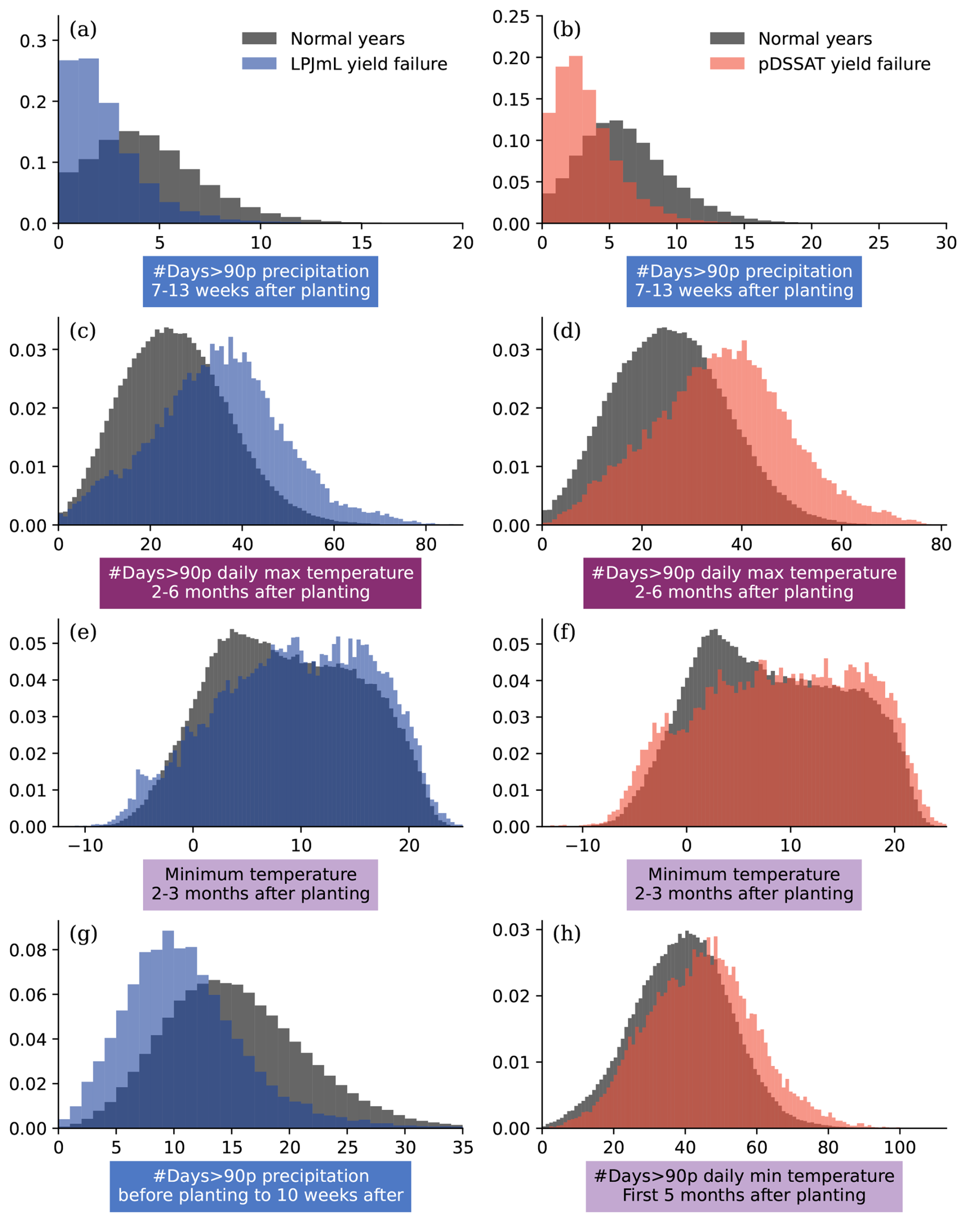
Histograms of some identified climate drivers in yield failure and non-yield failure years for each model are largely in agreement with the associations implied by the odds ratios (Fig. 6). For both crop models, yield failure years are more likely to have fewer rainy days between 7 and 13 weeks after planting (Fig. 6a and b) and more days of high maximum temperatures between 2 and 6 months after planting (Fig. 6c and d). Normal years are more likely to experience a lower minimum temperature during the second and third month after planting (Fig. 6e and f). For LPJmL, a higher number of rainy days in the first ten weeks after planting and eight weeks before are associated with decreased chances of yield failure (Fig. 6g). For pDSSAT, the yield failure distribution of the number of warm days (in which minimum daily temperatures exceed the 90th percentile) in the first five months after planting is slightly higher than normal years (Fig. 6h).

Figure 6 Distributions for normal and yield-failure years of some of the identified climate drivers of maize yield failure shown in Fig. 5, for LPJmL (a, c, e, g) and pDSSAT (b, d, f, h).

4.3 Our method robustly identifies plausible climate drivers that outperform many baseline feature sets

To evaluate the robustness of the approach we now turn to the results for the 100 bootstrap repeats, where in each repeat 20 pools are sampled from 100 total pools of candidate features. The original pools, by definition, contain an equal number of features based on each of the ten climate variables (Step 1). After selecting ten features from each pool based on cross-validation predictive performance (Step 2) we find that the majority of features selected consist of variables that are used as input by the crop models (Figs. A4a and A5a). However, some variables not used by the crop models are also selected, albeit less frequently (surface pressure, windspeed, and specific humidity for pDSSAT and surface pressure and specific and relative humidity for LPJmL).

After condensing the features selected from twenty pools to final sets of ten climate drivers (Step 3), variables not used as input by the crop models are eliminated for pDSSAT in all 100 bootstrap repeats (Fig. A4b), and for LPJmL, two of the variables not used by the crop model (specific humidity and surface pressure) are each selected in 3 out of 100 repeats, while the remaining variable unused by the crop model (relative humidity) is eliminated for all repeats (Fig. A5b). This shows that our approach is able to identify climate drivers based on variables that are used as input by the crop models and are therefore more plausibly causally-related to crop failure. When yields are detrended, results differ by crop model. For pDSSAT, specific humidity, which is not used as input by the crop model, appears in 97 of the 100 bootstrap repeats, relative humidity appears in three, and surface pressure is eliminated (Fig. B6a and b). For LPJmL, all variables not used by the crop model are eliminated for all bootstrap repeats (Fig. B7a and b).

The duration of the time intervals over which climate conditions are aggregated in the selected features before condensing (Step 2) displays three peaks: at two to four weeks, at two to three months, and at approximately four to five months. This third peak gradually tapers off, with some selected features based on ten or eleven months of climate data. The time intervals over which condensed drivers are aggregated (Step 3), on the other hand, show two distinct peaks for pDSSAT: at approximately eight weeks, and at four to five months (Fig. A4c). For LPJmL, the second peak, if present, is less visible (Fig. A5c). Drivers never, or rarely, consider more than six months of climate data. The differences between selected features and the condensed drivers identified are consistent when yields are detrended (Figs. B6c and B7c).

For both crop models, Lasso logistic regression models using sets of 5, 10 or 15 identified climate drivers, fitted on training data only, are able to achieve evaluation scores on the temporal, spatial and spatiotemporal test sets consistently higher than those using average growing-season or quarterly climate features and five extreme indicators (Figs. 7 and A6–A9). For pDSSAT, models using only ten identified climate drivers consistently perform better in terms of all performance metrics evaluated and on all test sets than any of the baseline feature sets tested. Models using only five drivers also outperform the baseline feature sets for most metrics and test sets; the only exception is the spatial held-out set, on which one baseline set is able to achieve a higher log loss score (although obtaining worse performance according to the three other performance metrics). For LPJmL, models using five or more drivers outperform all baseline feature sets on all test sets and for all evaluation metrics evaluated, with the exception of the baselines consisting of monthly climate aggregates, which achieve roughly similar scores (depending on the test set and evaluation metric used). For both crop models and all metrics, increasing the number of identified climate drivers used as predictive features is beneficial for model performance on the temporal test set, but can lead to unchanged or decreased performance on the spatial and spatiotemporal test sets (depending on the test set, crop model and evaluation metric used).

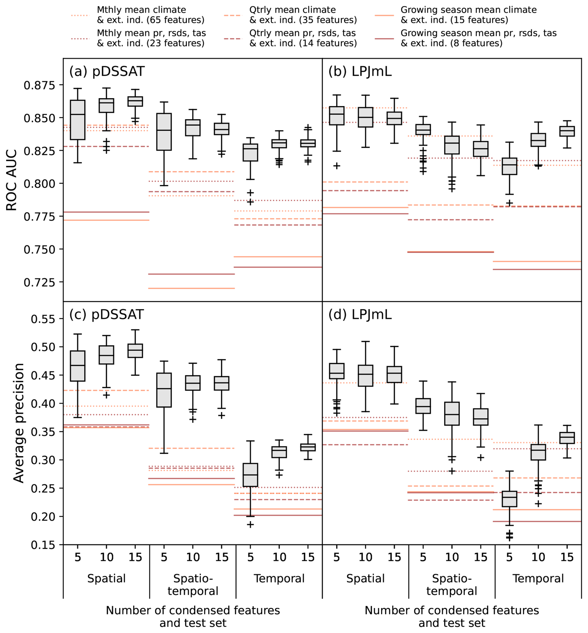
Figure 7 Comparison of the spatial, spatiotemporal and temporal test-set performance of Lasso models for pDSSAT (a, c) and LPJmL (b, d). Box plots show the scores for models using sets of five, ten or fifteen drivers using our proposed method, and horizontal lines denote the scores for the same models using baseline feature sets as predictors (made up of mean aggregate climate variables over the growing season or in monthly/quarterly intervals as well as five extreme indicators).

If second-order interaction terms are included, models using fifteen identified climate drivers can often outperform, or perform similarly to, models using monthly climate averages on the temporal test set for all evaluation metrics calculated, and can consistently outperform all other feature sets tested (Figs. A6–A9). On the spatial and spatiotemporal test set, models using identified drivers reliably outperform baseline sets consisting of annual climate averages plus extreme indicators, and outperform quarterly baseline sets according to most metrics evaluated. The comparison to baseline sets consisting of monthly climate averages plus extreme indicators depends on the crop model and evaluation metric used. Results are similar when using more complex extra trees models, and for both crop models and all models tested when yields are detrended (Figs. B8–B11).

The results described so far are based on applying the method to identify drivers of yield failure, where yield failure is defined as yields below the 10th percentile of those occurring during the training years. When reproducing the results using a more extreme (5th percentile) or more moderate (15th percentile) definition of yield failure, we find that the variables, aggregations and time-durations of identified drivers are largely identical, with some minor differences. In general, the results suggest that the method is slightly better able to eliminate variables that were not used as input for the crop models when using higher (more moderate) thresholds for defining yield failure. For example, when using a 5th percentile threshold, specific humidity is sometimes identified as a driver for LPJmL, but not when the 10th or 15th percentile is used.

The ten identified drivers based on 100 repeats are largely similar for all yield failure thresholds tested (Figs. C1–C2). In particular, the precipitation drivers and those using the number of days where maximum temperature is above the 90th percentile are almost identical. Almost all drivers identified are based on precipitation, minimum or maximum daily temperatures at different stages of the growing season. However, there are some differences, particularly in the drivers identified based on the 5th percentile, which features long-wave radiation for pDSSAT and specific humidity for LPJmL.

If a more extreme definition of yield failure is used (5th percentile), we observe generally poorer predictive performance across the held-out test sets, particularly in terms of average precision, for all models, whether using identified drivers or baseline climate feature sets (Fig. C3). This is likely because the task and the training set becomes more imbalanced, by definition, with fewer examples of yield failure. Correspondingly, when using a (more moderate) 15th percentile threshold, we observe overall higher scores across the models, metrics and test sets (Fig. C4). When comparing the relative performance of models using our drivers to those using baseline feature sets, however, the results are essentially unchanged for all thresholds: models using drivers identified using our proposed method as predictive variables usually outperform those using standard sets of climate indices.

Finally, we find that the results of the method are sensitive to the cross-validation method used when selecting features in Step 2, both in terms of climate variables selected and the test performance of models using sets of identified drivers. Using temporal cross-validation results in the highest proportion of potentially-causal variables used in features selected from pools (Step 2) and in identified drivers (Step 3), and this is consistent for both crop models (Figs. D1 and D2) and also when yields are detrended (Figs. D3 and D4). Spatial cross-validation and feature-cluster cross-validation results in a lower proportion of potentially-causal variables across all settings, and random cross-validation the lowest. Similarly, identified driver sets selected using temporal cross-validation in general achieve the highest test scores and those selected using random cross-validation the lowest (Fig. D5). This general behaviour is robust to the evaluation metric, the model used (Lasso logistic regression with and without second-order interactions or extra trees), the crop model and if yields are detrended.

In comparison to the choice of cross-validation strategy, the performance of the identified driver sets is relatively insensitive to all other parameters tested. Increasing the number of time intervals sampled per pool slightly improves model performance with resulting sets of drivers for pDSSAT, but not LPJmL. Interestingly, selecting fewer features from each pool leads to increased performance of identified driver sets in Step 3.

4.4 Meaningful and predictive drivers of yield failure are obtained by applying the method to observational data

Using the same methodology for observational US county-level data and daily meteorological data from eight variables, we obtain four climate drivers of maize yield failure (Fig. 8). The only variables used are precipitation, maximum vapour pressure deficit and maximum temperature, and the drivers cover a time period starting approximately one month before planting until around six months afterwards. Precipitation is relevant for a three-month period starting one month prior to planting, and the number of days in which the maximum temperature exceeds the 90th percentile are relevant from one month from planting until six months from planting. Two drivers are based on vapour pressure deficit conditions in two distinct phases of the growing season and based on different aggregation methods, with the number of days of extreme vapour pressure deficit conditions most relevant for a two-month period starting approximately two months after planting.

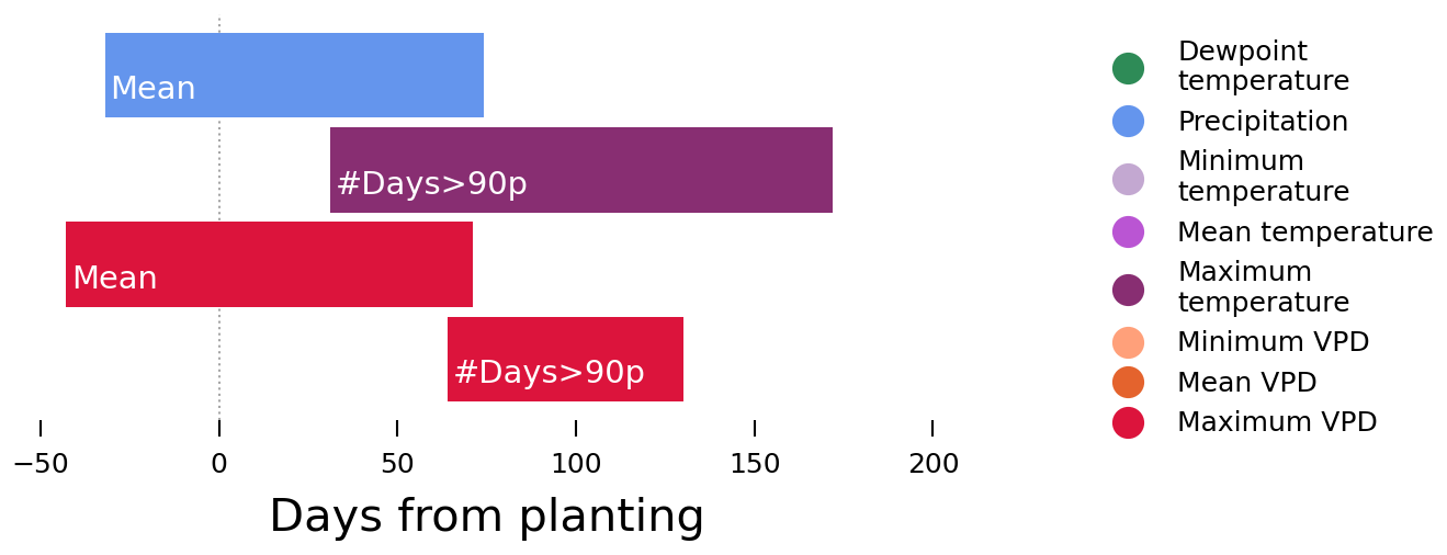
Figure 8 Four identified climate drivers of US county-level maize yield failure, for predominantly-rainfed counties, based on using 20 sampled time periods to generate 100 pools of candidate features, using ten-fold temporal cross-validation to select ten features from each pool, and condensing the resulting 1000 features.

A logistic regression model with the identified four drivers as predictors, fitted to data from the training years, achieves a test ROC AUC score of 0.85, average precision of 0.54, Brier score of 0.073 and log loss of 0.26, and the Pearson correlation of predicted versus ground truth annual proportions of counties experiencing yield failure is 0.98 (Fig. 9). Notably, the test years include a year which was heavily impacted by drought (2012), which is well-captured by the model (achieving an average precision in that year of 0.83).

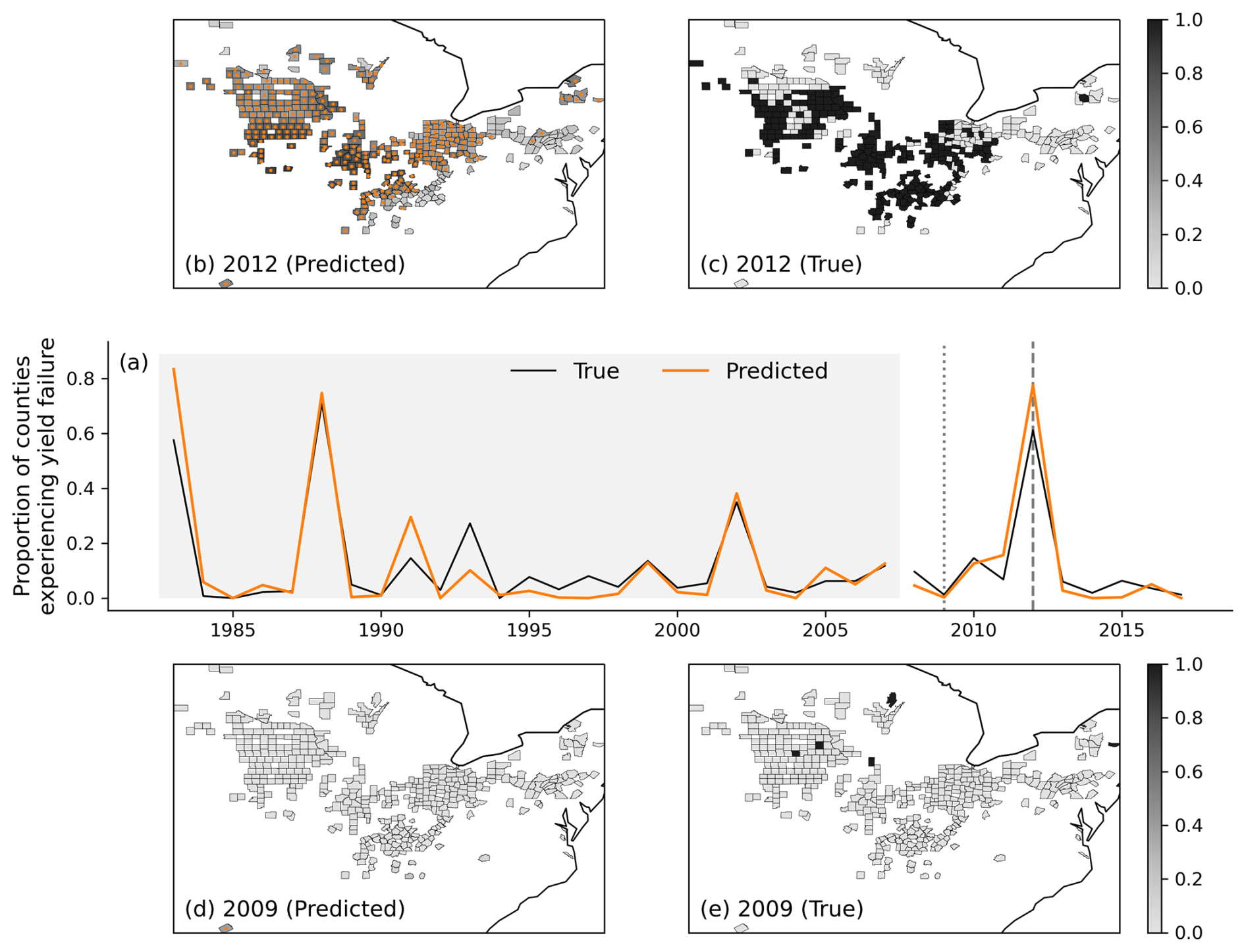
Figure 9 Temporal and spatial predictions of a logistic regression model using four identified drivers using observational county-level data. (a) True (black) and predicted (orange) proportion of counties experiencing yield failure each year. The dashed vertical line denotes the year in which the highest average precision is achieved, 2012, and model predictions for this year are illustrated in panel (b). Orange dots mark counties where yield failure is predicted by the model based on a threshold determined over the training years, and the corresponding ground truth is shown in panel (c). The dotted vertical line in panel (a) marks the year in which the lowest average precision is achieved, 2009, and the corresponding predictions and ground truth are shown in panels (d), (e) respectively.

5 Discussion and Conclusions

Identifying simple climate drivers from high frequency meteorological data that are associated with impacts is a challenging task. Most studies so far rely on selecting from a large set of predefined aggregate features in combination with statistical models (Ben-Ari et al., 2018; Vogel et al., 2021; Anand et al., 2024b; Heilemann et al., 2024). The choice of aggregation strategy and climate features used can significantly impact model performance and behaviour (Chen et al., 2024). Other studies use complex machine learning approaches to derive a mapping from meteorological conditions to impacts, but can struggle to obtain useful interpretations (Wolanin et al., 2020; Anand et al., 2024a). Our approach addresses this challenge in an efficient way. We generate many candidate features based on random time slices of the meteorological data, and use a robust, two-stage selection and synthesis process to extract a small set of drivers. While the method exploits the flexibility of ML models and the information contained in high-resolution, multivariate data, the resulting drivers are simple and consist of single climate variables aggregated over defined time intervals. We are then able to construct parsimonious logistic regression models using these drivers that are easy to interpret and have very high accuracy.

Our method identifies robust drivers in two stages: first, features are selected from large pools of candidates based on cross-validation performance; second, the selected features from all pools are clustered based on similarity and drivers are extracted from each of the largest clusters. The first stage is similar to methods that have been shown to improve model transferability in previous studies (Ludwig et al., 2023; Sweet et al., 2023). Our results suggest that the second stage, a novel contribution of this study, is also needed to reliably obtain climate drivers using only variables that are taken as input by the crop models. Interestingly, it also dramatically reduces the proportion of features lasting less than one month or more than six months. This second stage could be interpreted as obtaining drivers that are useful in combination with varying sets of other predictors, and that are robust to variation in start and end dates. Lischeid et al. (2022) found that machine learning models of yield variability using different predictor sets were able to achieve equally-good performance scores, and concluded that expert judgement was needed to identify the most reliable models. Our approach is, perhaps, a way of overcoming this challenge.

The predictive performance of models on held-out years and the consistency of identified relationships in different time periods can be used as evidence for a causal link, as has been done for instance by Schlenker and Roberts (2009) to show nonlinear temperature effects on different crop types. Our approach is motivated by a similar argument: climate indices that robustly improve model performance at predicting an impact in held-out years or locations are more likely to be causal drivers. Using yield simulations and their corresponding forcing data allows us to test this in a situation where some climate variables, such as humidity, are not taken as input by the crop models (and therefore do not have a causal effect on yields), but are still associated with the target variable due to dependencies between climate variables (as shown in composite plots). Additionally, each crop model uses a different subset of variables. The fact that the drivers identified by our method consistently consider only the climate variables taken as input by each crop model, despite the presence of strong associations between other variables and yield failure, is encouraging.

Many variables which influence agricultural yield are correlated in space and among themselves, which can lead to errors in empirically-estimated relationships. Climate change causes warmer temperatures and shifts in precipitation patterns, strongly affecting agricultural regions (Lobell and Di Tommaso, 2025). Data-driven models have difficulties extrapolating outside of the observed distribution, which could impede their use for projecting impacts under future climate change scenarios. The robustness of our results, despite the challenging split between training and test years and regions used in this study, show that our approach is successful in tackling these challenges. Data-driven emulators of process-based crop models have been proposed to efficiently downscale simulations and facilitate the creation of large ensembles of agricultural projections in different climate scenarios. Published emulators of crop models have used predictors such as the mean and standard deviation of temperature and precipitation over the growing season or per month, and measures of climate extremes such as the number of extreme degree days or the maximum consecutive days with no rainfall (Folberth et al., 2019; Liu et al., 2023). However, due to the presence of spatiotemporal autocorrelation in the data used for training these models, emulator skill has been found to drop sharply when tested on held-out years or locations (Liu et al., 2023; Sweet et al., 2023). Our approach, on the other hand, identifies a set of climate features that are robust drivers of a specific impact or metric and can be used to create a lightweight, interpretable model that achieves high performance on datapoints many decades after the training period or in unseen latitudes. Such emulators or metamodels could also be used to analyse the processes leading to specific model outcomes which might emerge from the interaction of multiple complex mechanisms and therefore not be well-understood. Our results also show that our method is robust to the percentile threshold used for defining yield failure. This suggests that the method could be used by researchers to differentiate between drivers of more extreme or more moderate climate impacts, which could be caused by different processes.

Our method is robust to the majority of parameters tested, with the exception of cross-validation strategy used for selecting features from each pool (Step 2). This is in alignment with previous findings that feature selection and hyperparameter tuning is sensitive to this choice (Meyer et al., 2018; Sweet et al., 2023). It is noteworthy that, while in general we find that driver sets identified using temporal cross-validation perform better in held-out test years, and those using random cross-validation perform the worst, the difference in performance is quite small in comparison to the drastic difference in the climate variables used in features selected and sets of identified drivers. Random cross-validation has recently been used to identify parsimonious sets of weather drivers for modelling the effect of climate change on crop production accounting for adaptation (Hultgren et al., 2025). Given that the sets of weather drivers used in data-driven models can impact resulting agricultural projections (Chen et al., 2024), our results suggest that results from such methodologies may be sensitive to the cross-validation strategy used.

This study uses crop model simulations, which allow us to validate the predictive performance of drivers under challenging conditions and confirm that the variables used in identified drivers correspond to those used by the crop models, and are plausible based on our knowledge of their underlying mechanisms. For LPJmL, precipitation matters most in the juvenile phase of crop development, where leaf area index increases most steeply. Water stress during this phase can lead to permanent reduction in light interception, and thus yield penalty. Hot days (which are represented in our identified drivers counting the days above the 90th percentile of maximum daily temperature) can damage photosynthetic capacity if they are higher than an optimal threshold. However, these interpretations should be considered with caution. Both of the crop models used consist of multiple mechanisms that can interact in surprising ways, and the process by which we transform yields to yield failures is dependent on the grid cell and time period selected. This means that, even in this simulated setup, confirming that climate drivers identified by our approach are “accurate” is not straightforward. Furthermore, while we evaluate our method based on the principle that identified drivers should consider only the climate variables taken as input by each crop model, this does not take into account the fact that secondary variables not used as input may be internally estimated by the crop model using other information. For example, both crop models estimate potential evapotranspiration using the Priestley–Taylor radiation-based approach, which does not consider air humidity but implicitly represents atmospheric demand through available energy and an empirical coefficient. The match between selected and input variables is only one aspect of the method's fidelity, and should be considered in combination with the sensitivity of crop model processes used to compute yield to individual driver variables, and consistency of the identified drivers with the known underlying processes in terms of phenological timing and the aggregation strategy employed, as well as the climate variable used. However, these criteria are difficult to quantify, and require good understanding of the underlying crop model functionality to evaluate. Other formulations for potential evapotranspiration are employed in crop models (e.g. Cammarano et al., 2016) and applying the method to simulations from a more diverse set of crop models in general would likely find other variables as important. Out-of-distribution model performance can also provide evidence that drivers obtained are a good approximation for crop model behaviour.

While our results suggest that this method can generally identify robust and plausible drivers, its performance (like any data-driven approach) depends on task difficulty and data availability. This is illustrated when varying the threshold used to define yield failure. A more extreme definition (i.e, a 5th percentile threshold) means that the training set will contain fewer examples of yield failure, which could make it harder to identify robust drivers. This may explain why, for LPJmL, specific humidity (which is not an input to the crop model) is sometimes identified as a driver when using a 5th percentile threshold, but not for less extreme thresholds. Therefore, drivers identified at very extreme impact definitions should be interpreted with caution. One way to assess whether the identified drivers reflect genuinely different underlying processes at those levels is to compare their predictive performance against drivers identified using more moderate thresholds. If the drivers identified for more extreme events are spurious due to limited and imbalanced data, then drivers identified under easier conditions would likely perform better even when predicting more extreme events.

Detrending impact data introduces another layer of difficulty, as identical climate conditions can lead to yield failures in one year or location, but not in another, depending on yields experienced in previous years (Siebert et al., 2017a). Consistent with this, our results show generally degraded performance scores for all models (whether using identified drivers or baseline climate feature sets) for detrended data. In fact, even a perfect emulator of the underlying crop model could not achieve perfect predictive performance without access to information in previous years. As a result, spurious correlations may be more likely to achieve predictive skill and robustness comparable to that of true causal drivers. This could explain why specific humidity appears as an identified driver for detrended pDSSAT, but not in the non-detrended case. In line with this, we also find that as the yield failure threshold becomes less extreme (meaning the task becomes easier and the training set includes more examples of yield failure), specific humidity appears less frequently in the identified drivers. It is important to note that this reduction is much stronger for the identified drivers than for the features selected in the first step of the method, suggesting that the full method is still more reliable than sequential feature selection alone.

When moving to observational data, some additional challenges need to be considered. There might be sampling biases, for instance because farmers choose to plant crops in climatically-suitable regions or reduce harvested areas in years with adverse weather conditions. Furthermore, changing management practices, irrigation and crop breeding strongly affect crop yields, often exceeding trends related to climate change. Disentangling the influence of weather is also made more challenging as adaptation occurs in response to and in anticipation of climate change. When analysing weather effects on crop productivity, yields and/or climate variables are often detrended at each location in order to remove the influence of such longer-term shifts and focus on interannual yield variability. However, as noted by Siebert et al. (2017a), this leads to the implication that similar climate conditions can invoke completely different crop yield responses depending on the specific location and the climate conditions observed there in the dataset used for analysis. In this study we present the results obtained when applying the method to both non-detrended and detrended crop yields to explore the impact of this. In general, the climate drivers obtained and resulting model performances are similar in both settings, but some differences are present.

Despite these difficulties, by applying the method to reported county-level maize yields and eight corresponding meteorological variables, we obtain four climate drivers of maize yield failure that are physically plausible, and a simple logistic regression model using those predictors is able to capture the effects of the drought conditions of 2012. Vapour pressure deficit is identified as particularly relevant, with elevated levels later in the growing season found to be particularly relevant. This corresponds with the findings of Lobell et al. (2014), in which monthly aggregates of precipitation, vapour pressure deficit and minimum and maximum daily temperatures were used as candidate predictors for multivariate adaptive regression splines, and vapour pressure deficit in the third month after sowing identified as the most influential variable. High temperatures during the growing season (after the first month of plant development) are also identified as a driver of yield failure using our method. Increased temperatures and elevated vapour pressure deficit conditions both contribute to yield loss through separate mechanisms, but disentangling their effects can be challenging as the two factors are highly correlated and their impacts depend on precipitation levels (Hsiao et al., 2019). It is noteworthy that the logistic regression model is unable to capture the effects of the heavy rainfall conditions in 1993. This may be due to the inability of the variables used to capture the effects of soil moisture on yields. For example, Rigden et al. (2020) identified negative impacts to maize yields in the US Midwest when either vapour pressure deficit or soil moistures reached high levels. Future work could include soil moisture and other variables to explore these relationships further.

While model performance using the identified drivers over the studied period is good, and the identified drivers appear plausible, it is difficult to assess the robustness of the methodology on observational data. Crop yields are affected by many types of weather conditions during different times of the growing season, making it challenging to argue that any obtained drivers are not plausible in some way. In particular, our method identified climate drivers relative to the planting date, which were held constant in the simulations used for validating our method and assumed to be constant in the application to observational data. In reality, farmers may adjust their planting date in response to climatic and/or other conditions. While keeping planting dates constant could allow for capturing the impact of climate variability on yields via delayed or early planting, long-term trends in planting dates due to climate change would make interpretation of the results difficult due to confounding effects. Maize cropping areas in the US have experienced relatively little warming over the last half-century (Lobell and Di Tommaso, 2025), and although planting dates advanced between 1985 and 2005 (Sacks and Kucharik, 2011), no meaningful trend was observed over 2000–2020 (Deines et al., 2023). We therefore assume that shifts in planting dates would not have a significant impact on our results. However, this assumption may not hold in regions more affected by warming. Future work exploring the robustness of our proposed method to changing planting dates in response to climate change trends, or to uncertainties in planting date data, would be beneficial. Furthermore, observational data is only available over a limited period of time, during which agricultural practices have evolved, making robust model evaluation challenging. Therefore, while the strength of our results suggest that this approach could be applied to observation data, we advise conducting careful sanity checks and validating that the results are in agreement with scientific understanding. In conclusion, here we present an efficient and flexible approach to identify climate drivers associated with impacts. The identified drivers can be used as predictors in simple, interpretable models for further analysis, or could be used to guide experimental design for studying the effect of multiple stressors and different types of compound events, which otherwise may suffer from the curse of high dimensionality (Zscheischler et al., 2020; Webber et al., 2022; Kim et al., 2025). We test the approach on simulated crop yield data, show that it is robust to different parameter choices, and, finally, demonstrate the use of the method on observational data. While we illustrate the use of this approach for identifying drivers of maize yield failure, it could also be applied to other climate impacts that are influenced by weather events with different timings and durations, such as forest mortality, wildfire occurrence or flooding.

Appendix A: Supporting figures for non-detrended data

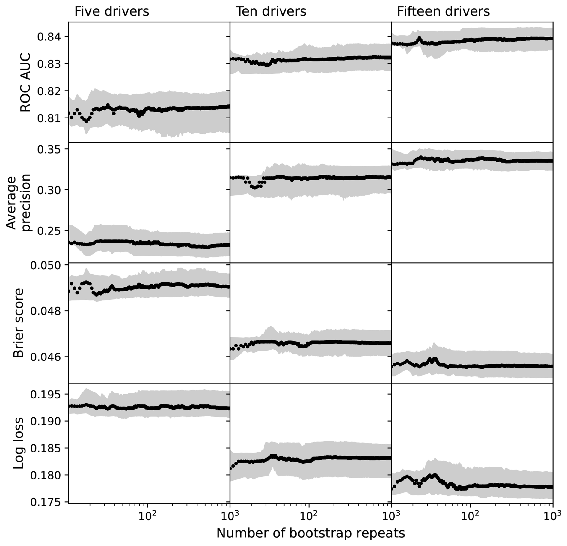
Figure A1 Stability of lasso logistic regression model performance estimates with increasing number of bootstrap repeats, using different numbers of identified climate drivers (columns) as predictive features, and using four different performance metrics (rows). Scores are calculated on the temporal test set, for non-detrended LPJmL. Black lines mark the median score across the repeats and the shaded region indicates the interquartile range.

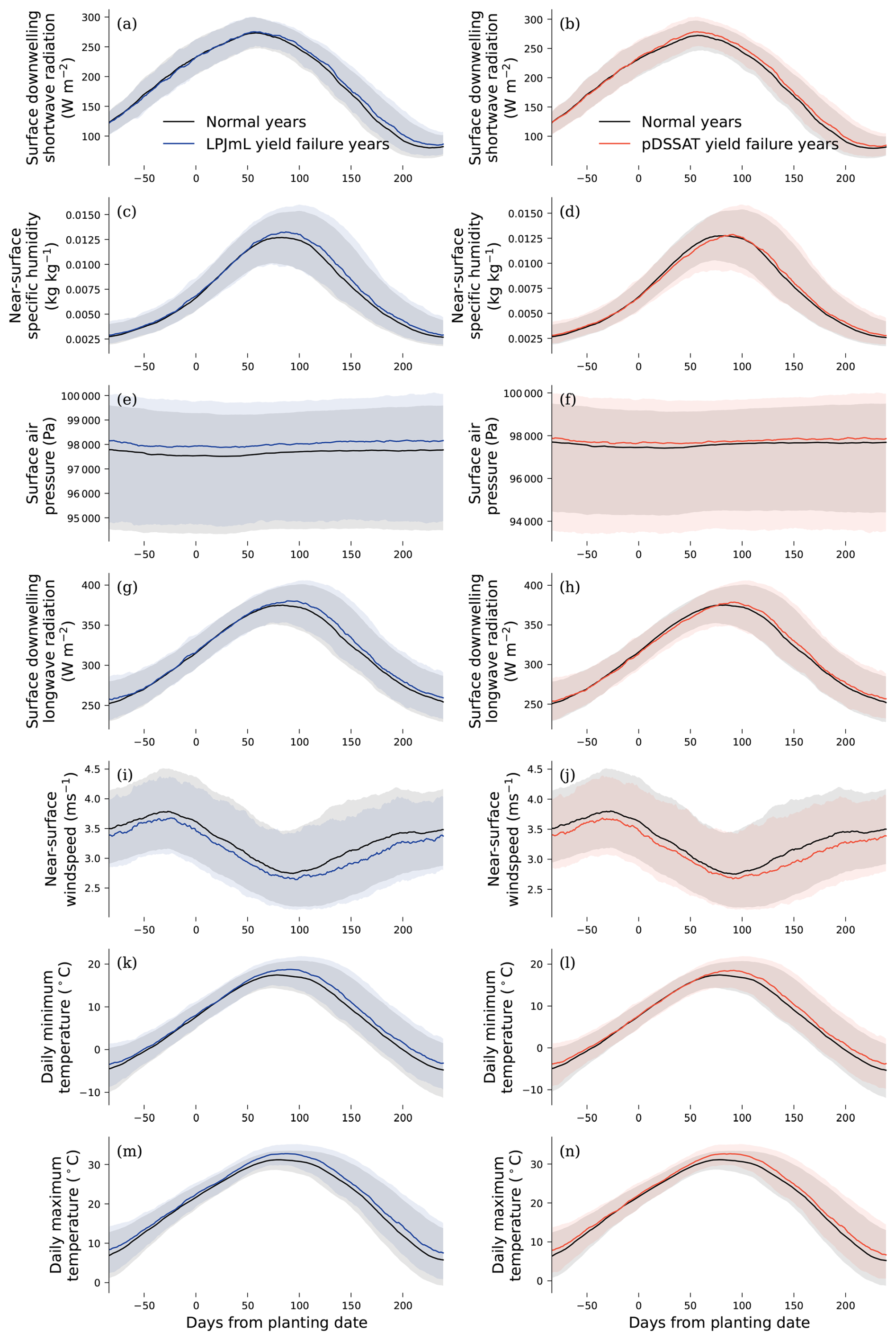
Figure A2 As in Fig. 3, composite plots of the seven-day rolling mean of surface downwelling shortwave radiation, near-surface specific humidity, surface air pressure, surface downwelling longwave radiation, near-surface wind speed, daily minimum temperature, and daily maximum temperature for LPJmL (a, c, e, g, i, k, m) and pDSSAT (b, d, f, h, j, l, n) for either normal years or yield failure years, without detrending.

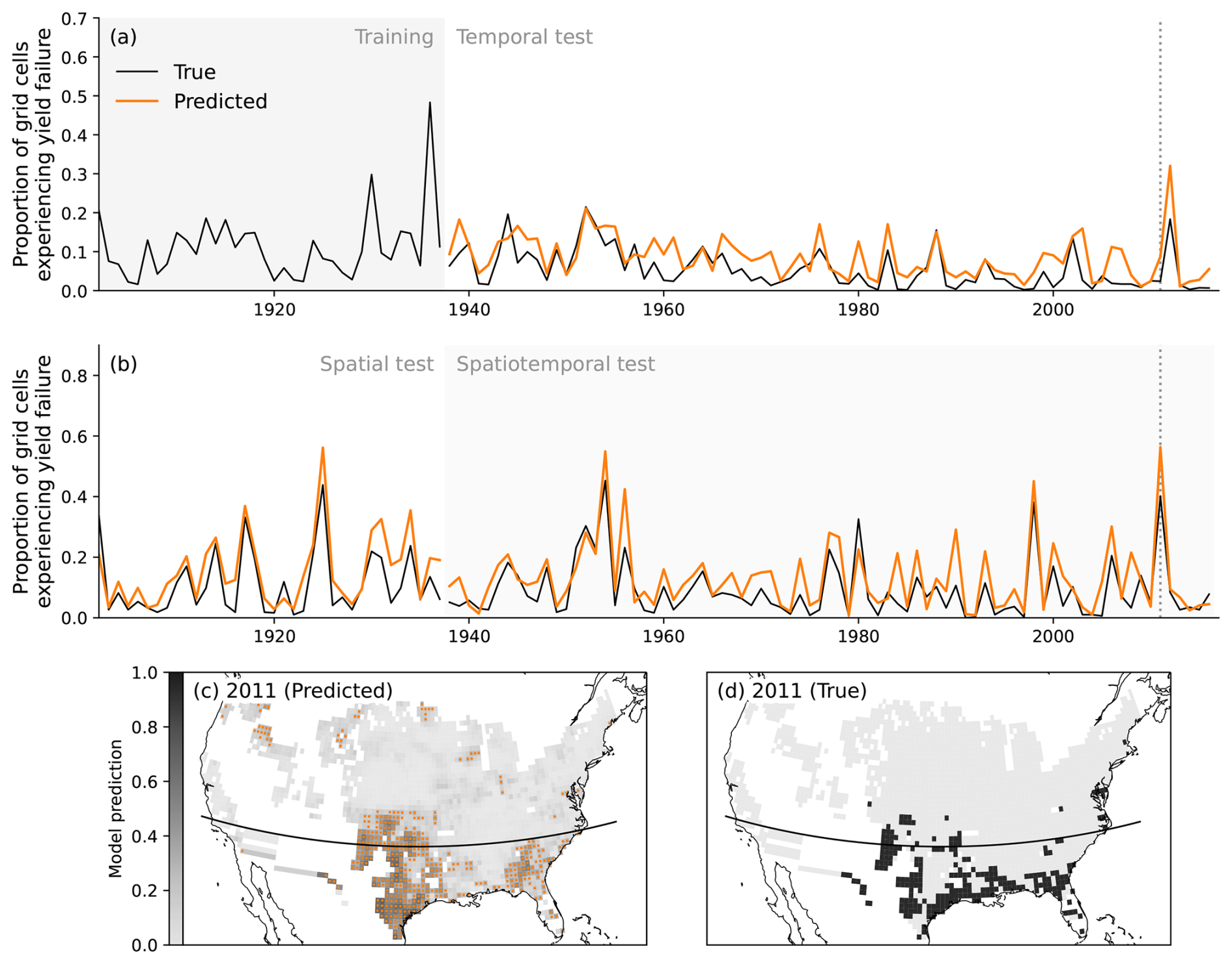
Figure A3 As Fig. 4 but for LPJmL. The threshold used for predicting yield failure years is 0.247, which achieves an f-score on the training set of 0.461.

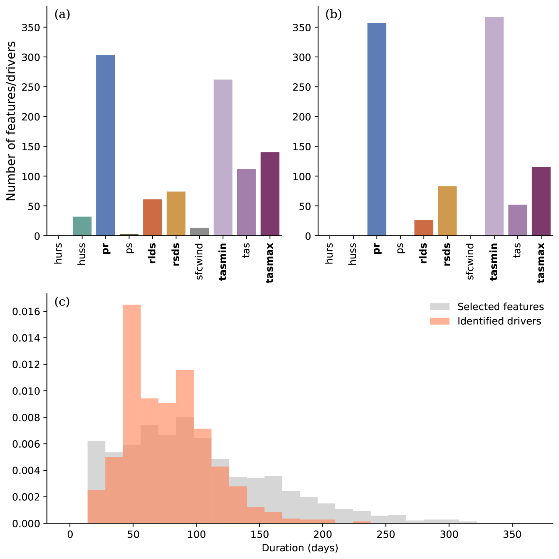
Figure A4 Climate variables used in features selected after Step 2 of our method (a) and in drivers identified from condensing those features in Step 3 (b), for pDSSAT without detrending. Bold text indicates variables used as input by the crop model: precipitation (pr, mm), surface downwelling longwave radiation (rlds, W m⁻²) and shortwave radiation (rsds, W m⁻²), daily minimum (tasmin, °C) and maximum near-surface air temperature (tasmax, °C). Not used by the crop model are near-surface relative humidity (hurs, %), near-surface specific humidity (huss, kg kg⁻¹), surface air pressure (ps, Pa), near-surface windspeed (sfcwind, m s⁻¹) and mean daily near-surface air temperature (tas, °C). However, pDSSAT does use minimum and maximum daily temperatures which are then downscaled to hourly values. The density histogram in panel (c) shows the duration in days of the resulting features or drivers at each stage.

Figure A5 As Fig. A4 but for LPJmL.

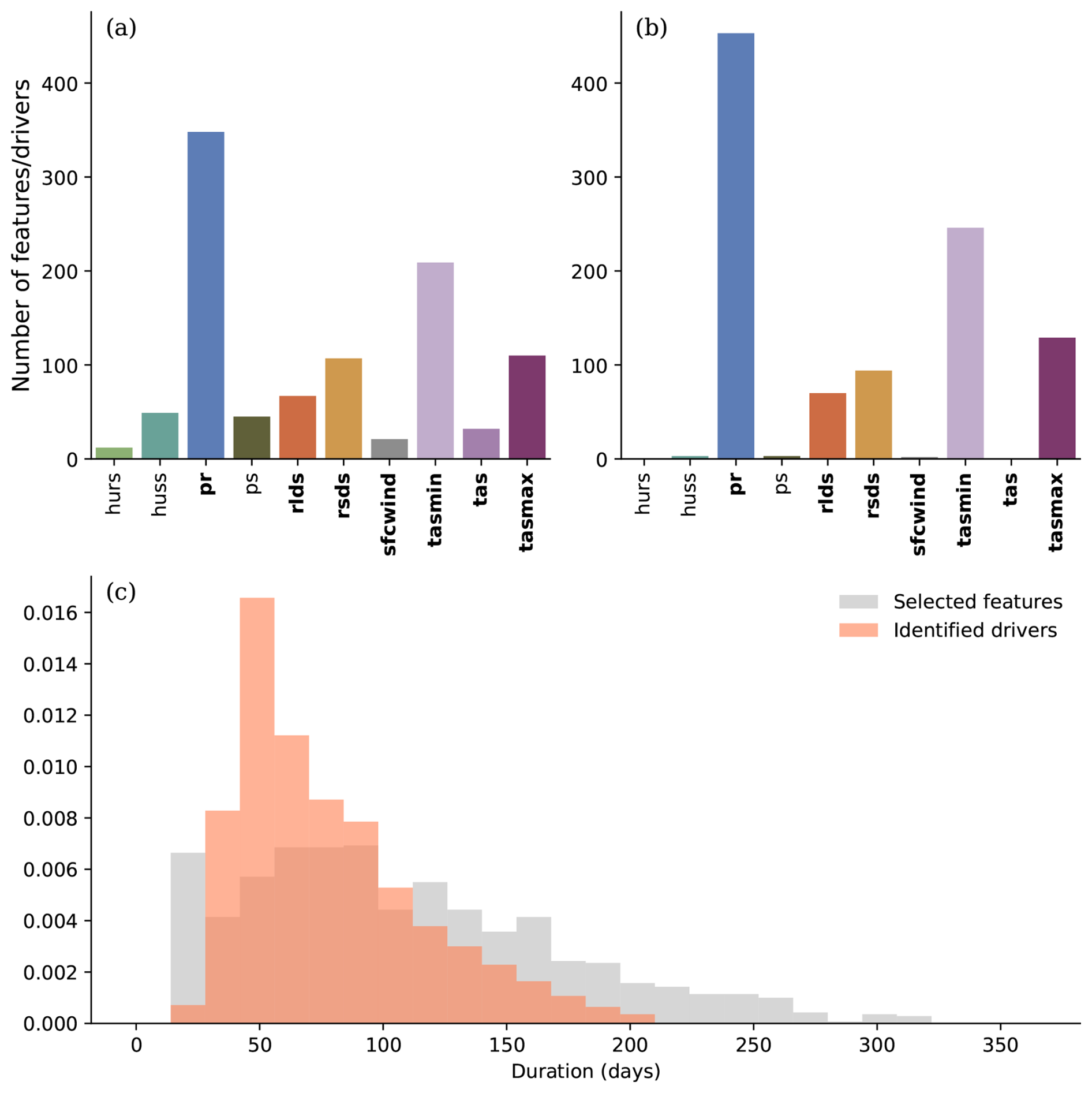
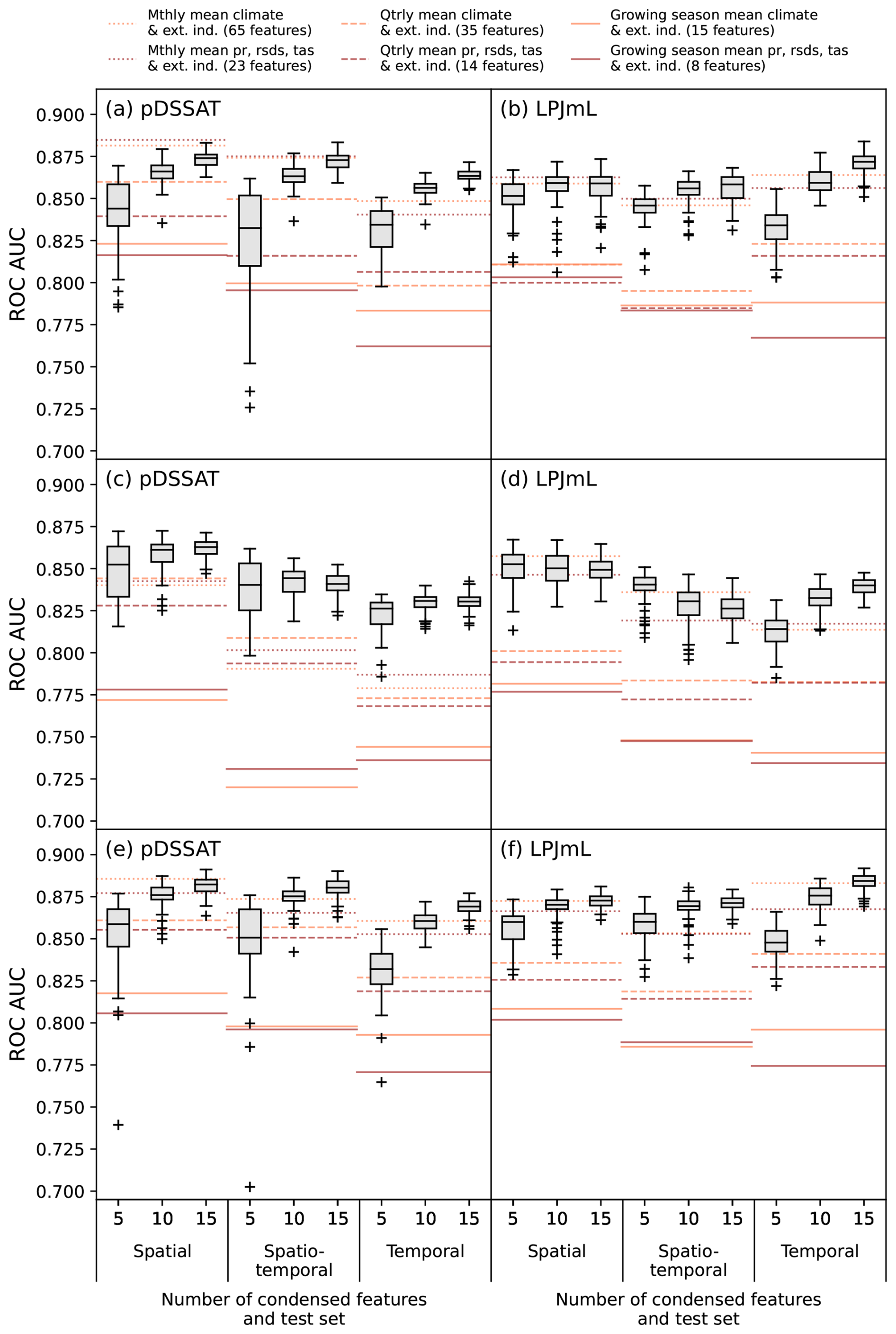
Figure A6 ROC AUC scores on test sets for models trained on training set, using feature sets derived from training set data (higher is better). (a, c, e) show scores for pDSSAT and (b, d, f) show LPJmL. (a, b) use LASSO logistic regression and include interaction terms; (c, d) use LASSO without interaction terms, (e, f) use extra trees.

Figure A7 As in Fig. A6 but for average precision (higher is better).

Figure A8 As in Fig. A6 but for Brier score (lower is better).

Figure A9 As in Fig. A6 but for log loss (lower is better).

Appendix B: Supporting figures for detrended data

Figure B1 As Fig. 3 but with yield failure years defined using detrended yields.

Figure B2 As Fig. A2 but for detrended yields.

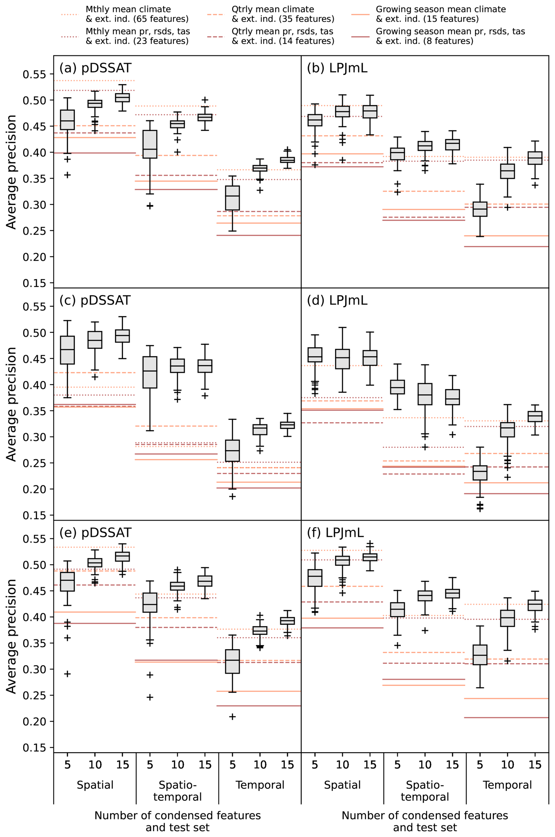
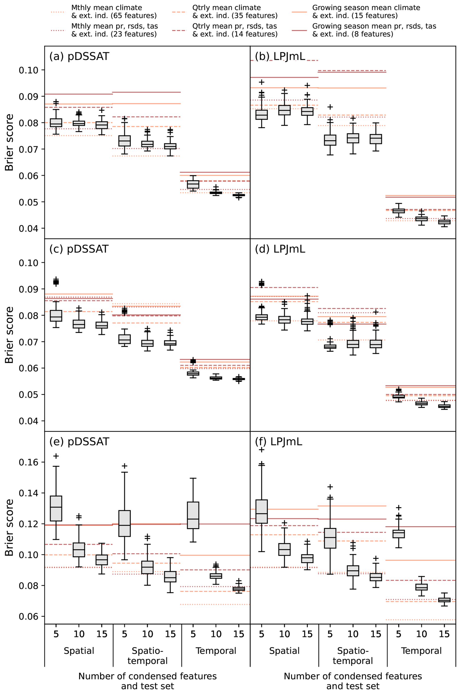
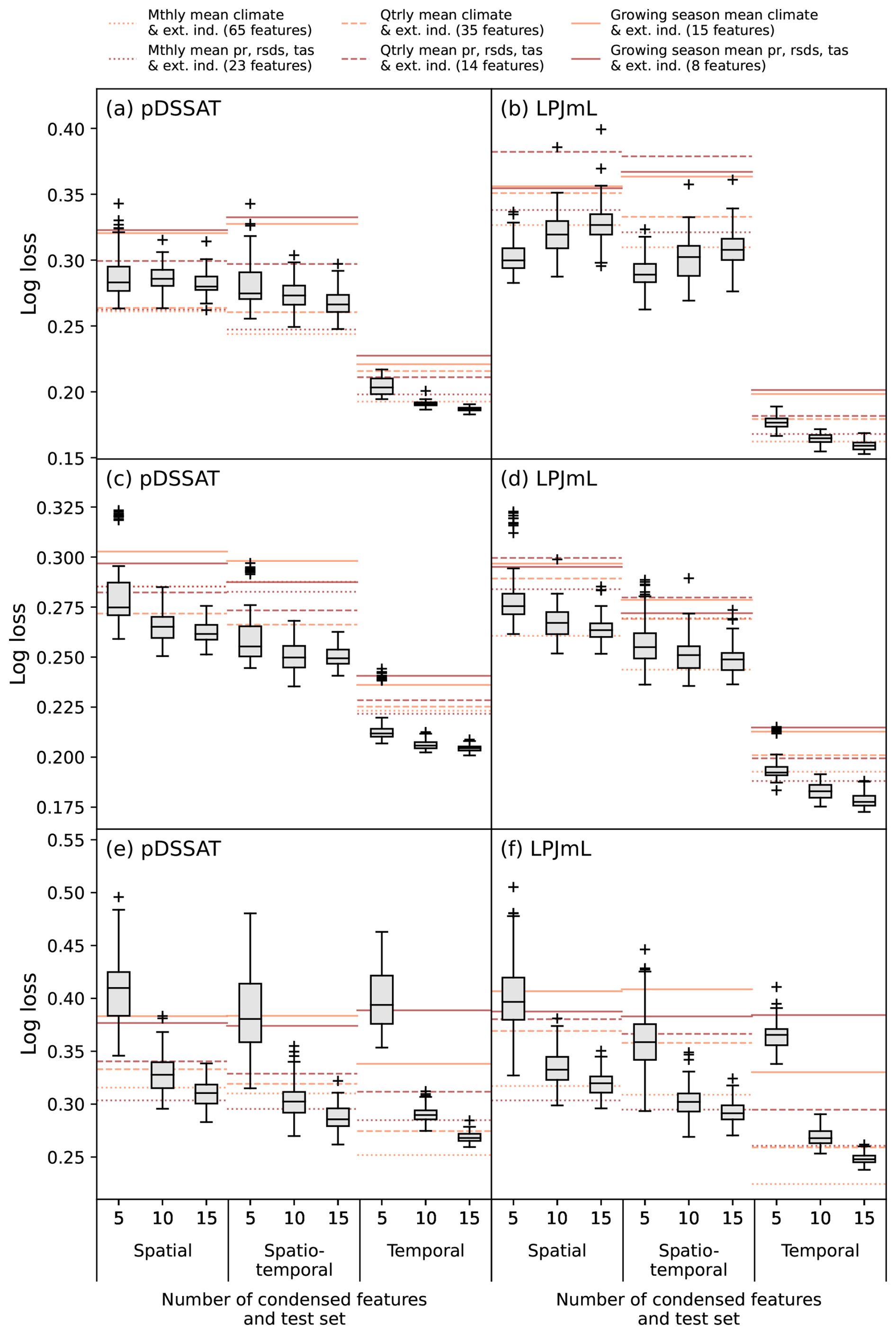
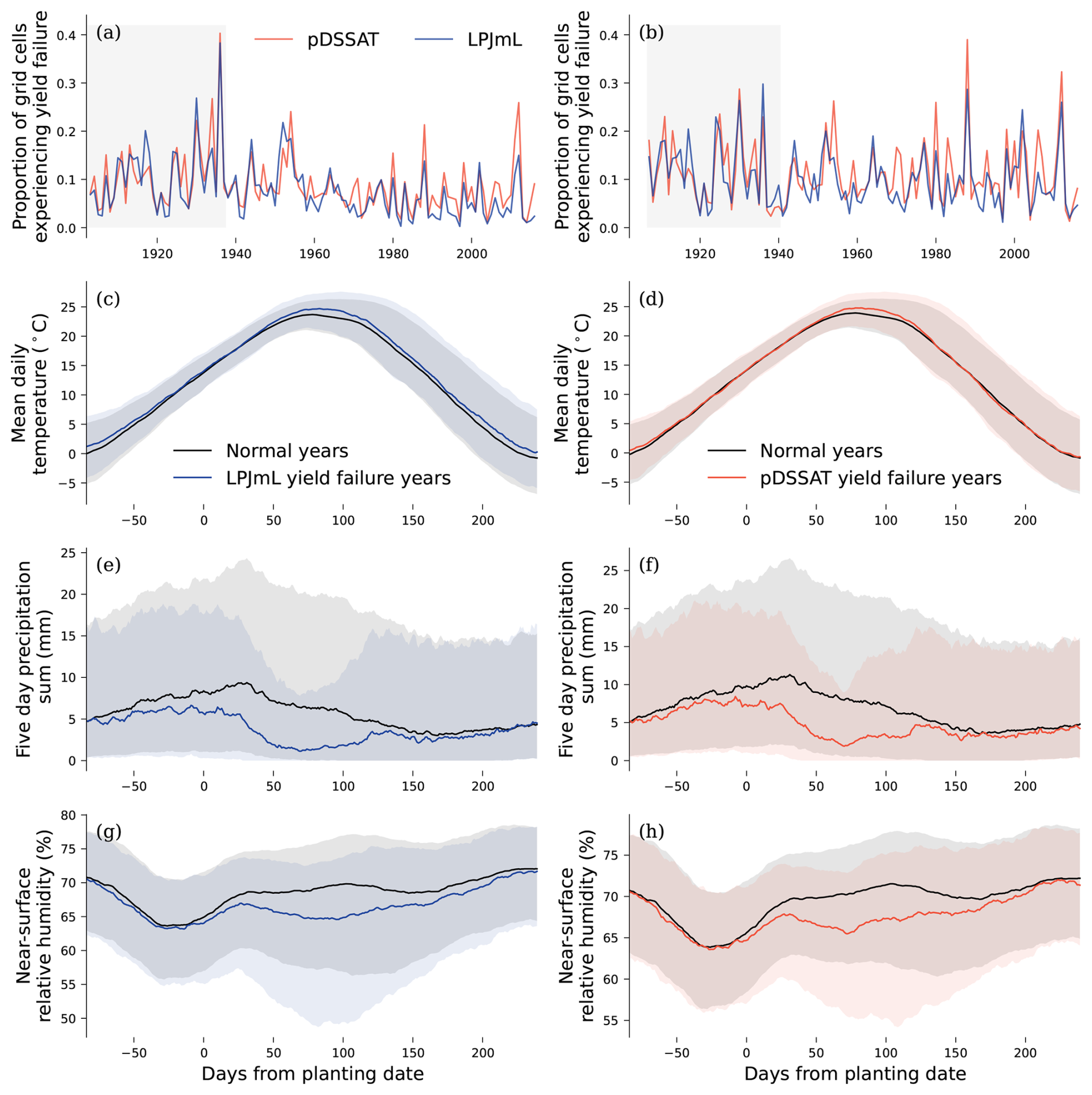
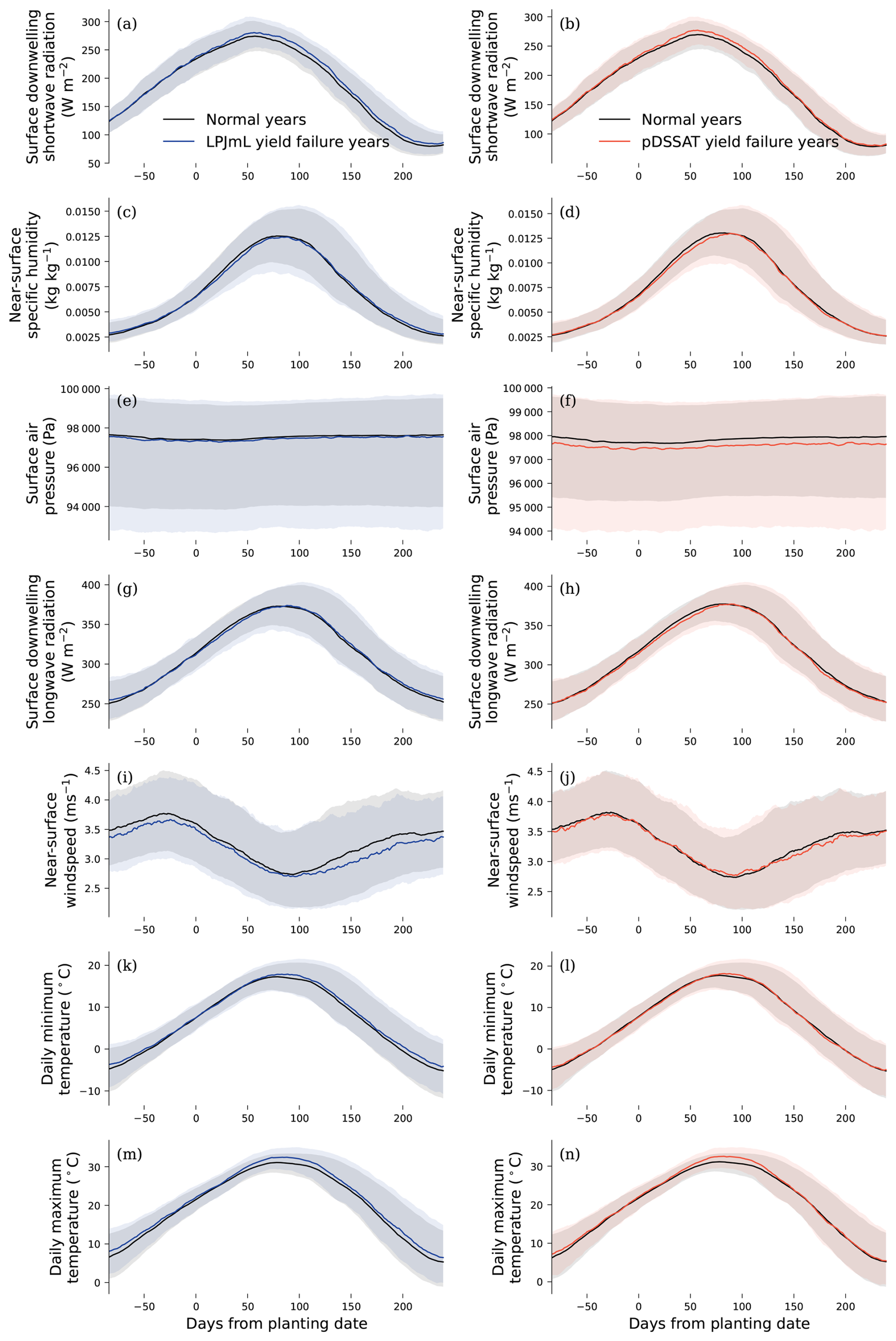
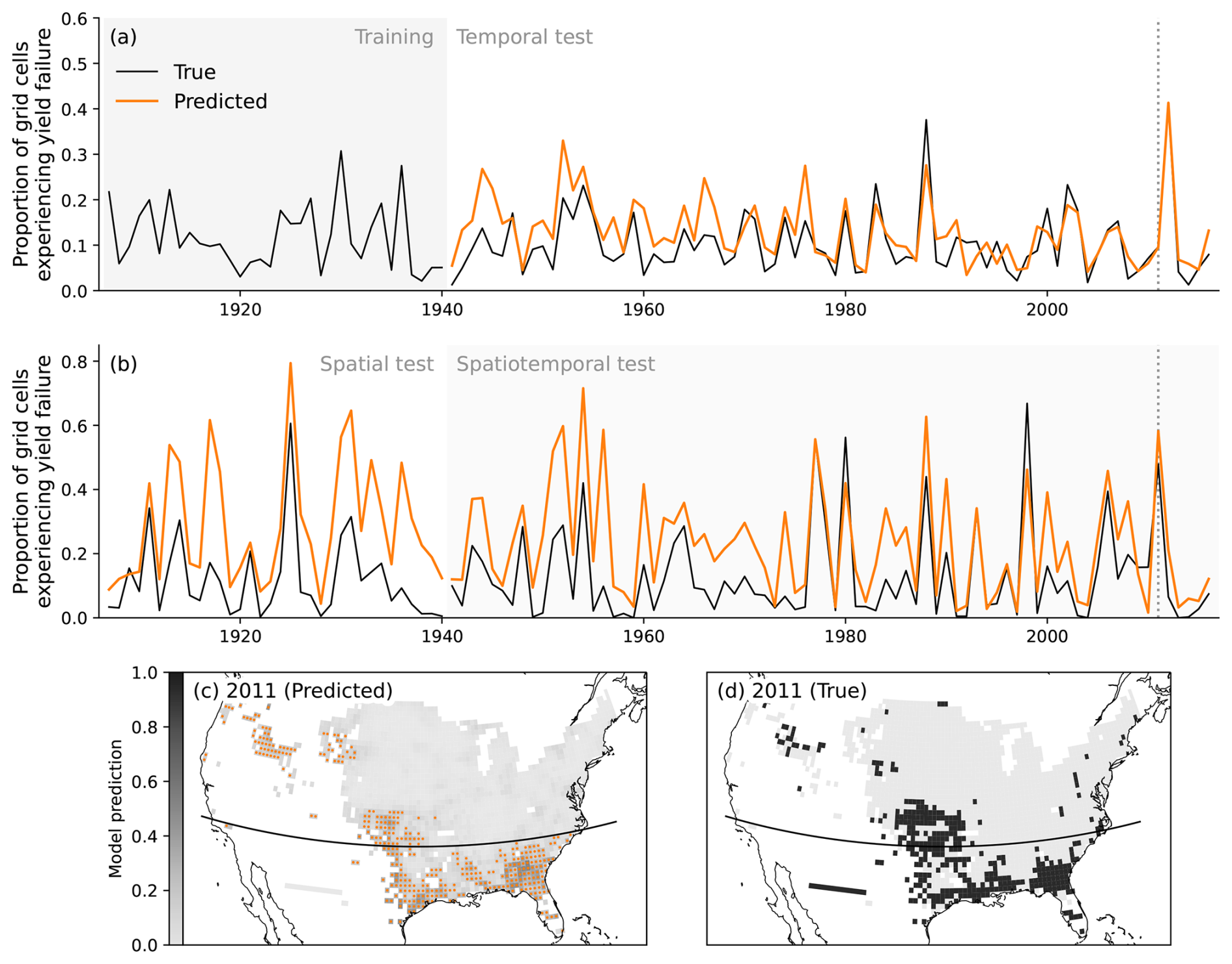
Figure B3 As Fig. 4, for pDSSAT after yields are detrended by removing the seven-year rolling average. The model achieves a ROC AUC of 0.80, average precision of 0.32, Brier score of 0.08 and log loss of 0.28 on the temporal test set, a ROC AUC of 0.85, average precision of 0.43, Brier score of 0.08 and log loss of 0.28 on the spatial test set, and a ROC AUC of 0.83, average precision of 0.42, Brier score of 0.09 and log loss of 0.31 on the spatiotemporal test set. The threshold used for predicting yield failure years is 0.194, which results in an f-score on the training set of 0.382. The Pearson correlation of predicted and true annual proportions of grid cells experiencing yield failure is 0.79 on the temporal test set and also 0.79 on the spatiotemporal test set.

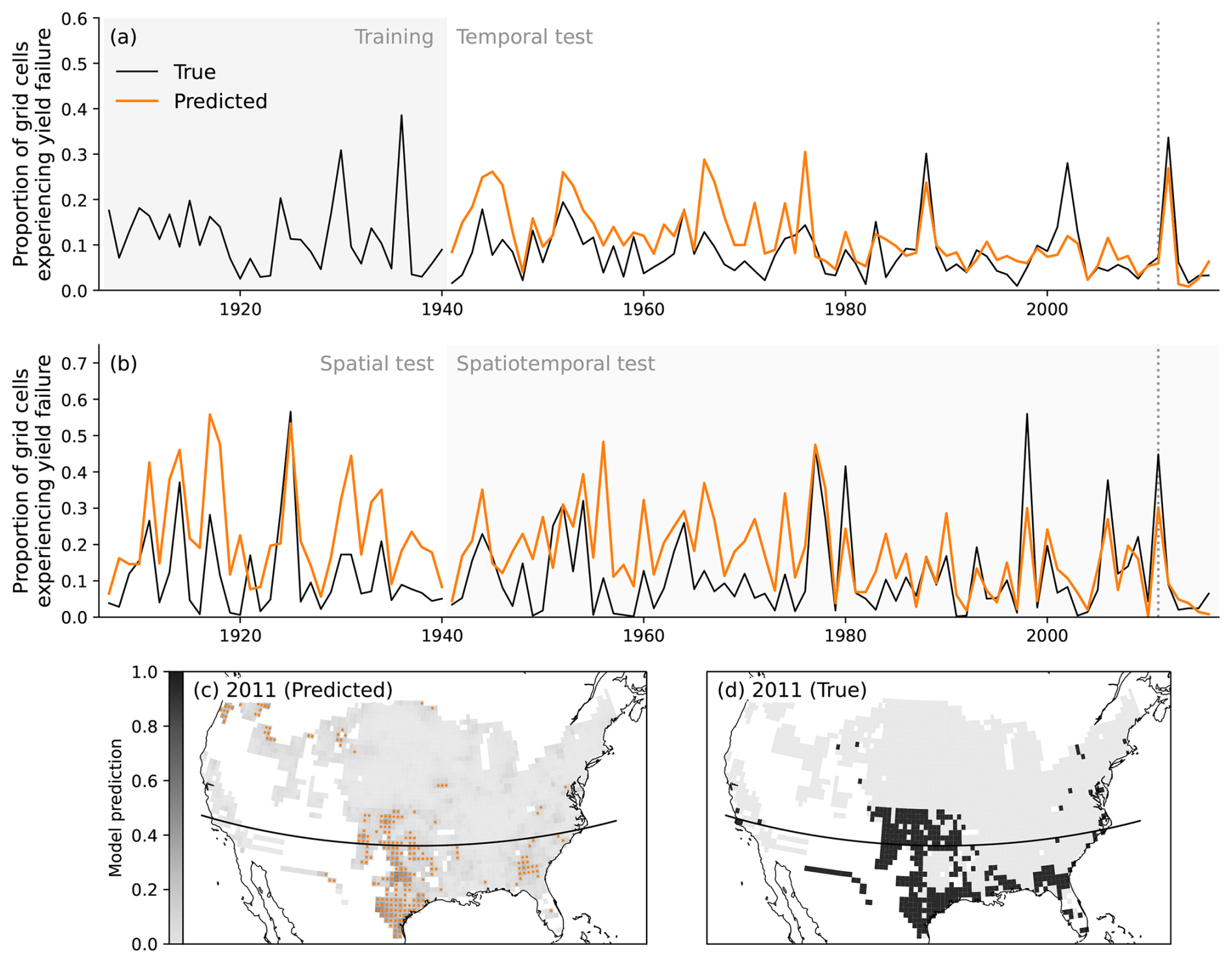
Figure B4 As Fig. 4, for LPJmL after yields are detrended. The model achieves a ROC AUC of 0.81, average precision of 0.31, Brier score of 0.07 and log loss of 0.24 on the temporal test set, a ROC AUC of 0.80, average precision of 0.36, Brier score of 0.09 and log loss of 0.31 on the spatial test set, and a ROC AUC of 0.78, average precision of 0.31, Brier score of 0.09 and log loss of 0.32 on the spatiotemporal test set. The threshold used for predicting yield failure years is 0.202, giving an f-score on the training set of 0.409. The Pearson correlation of predicted and true annual proportions of grid cells experiencing yield failure is 0.63 on the temporal test set and 0.64 on the spatiotemporal test set.

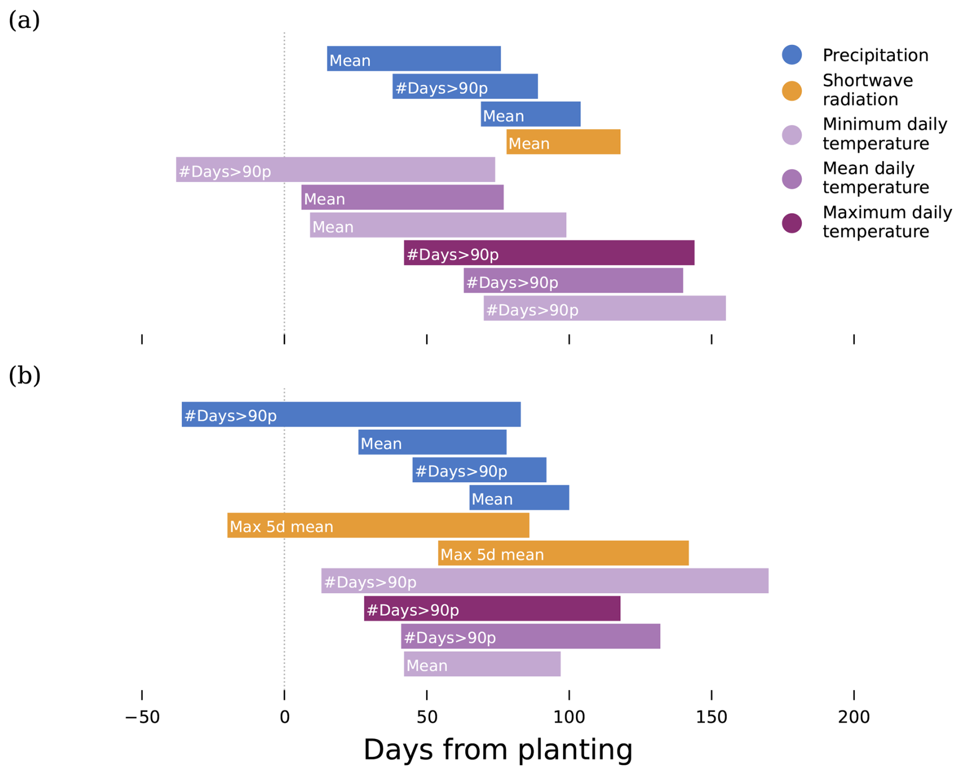
Figure B5 As Fig. 5, identified climate drivers of maize yield failure for (a) pDSSAT and (b) LPJmL when yields are detrended.

Figure B6 As Fig. A4, for pDSSAT when yields are detrended.

Figure B7 As Fig. A5, for LPJmL when yields are detrended.

Figure B8 As Fig. A6, when yields are detrended.

Figure B9 As Fig. A7, when yields are detrended.

Figure B10 As Fig. A8, when yields are detrended.

Figure B11 As Fig. A9, when yields are detrended.

Appendix C: Results using different thresholds to define yield failure

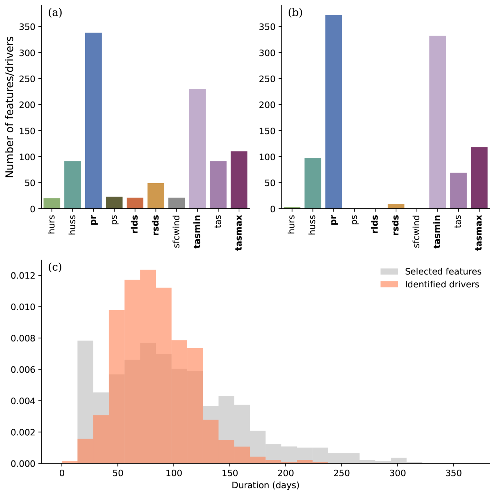
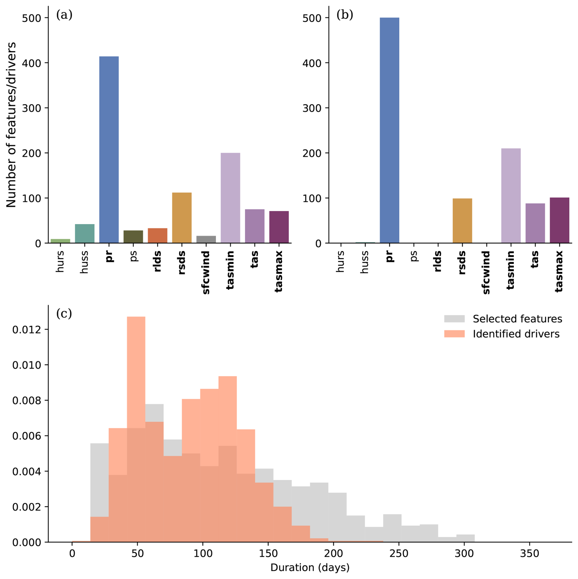
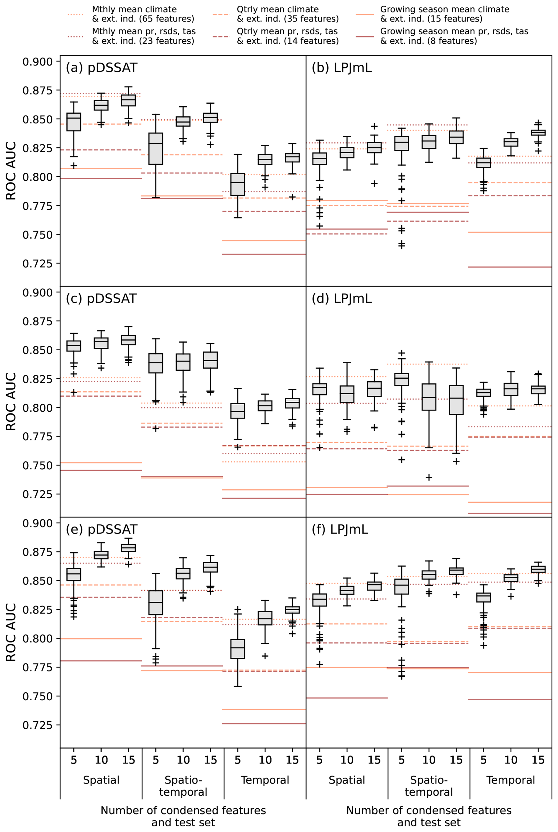
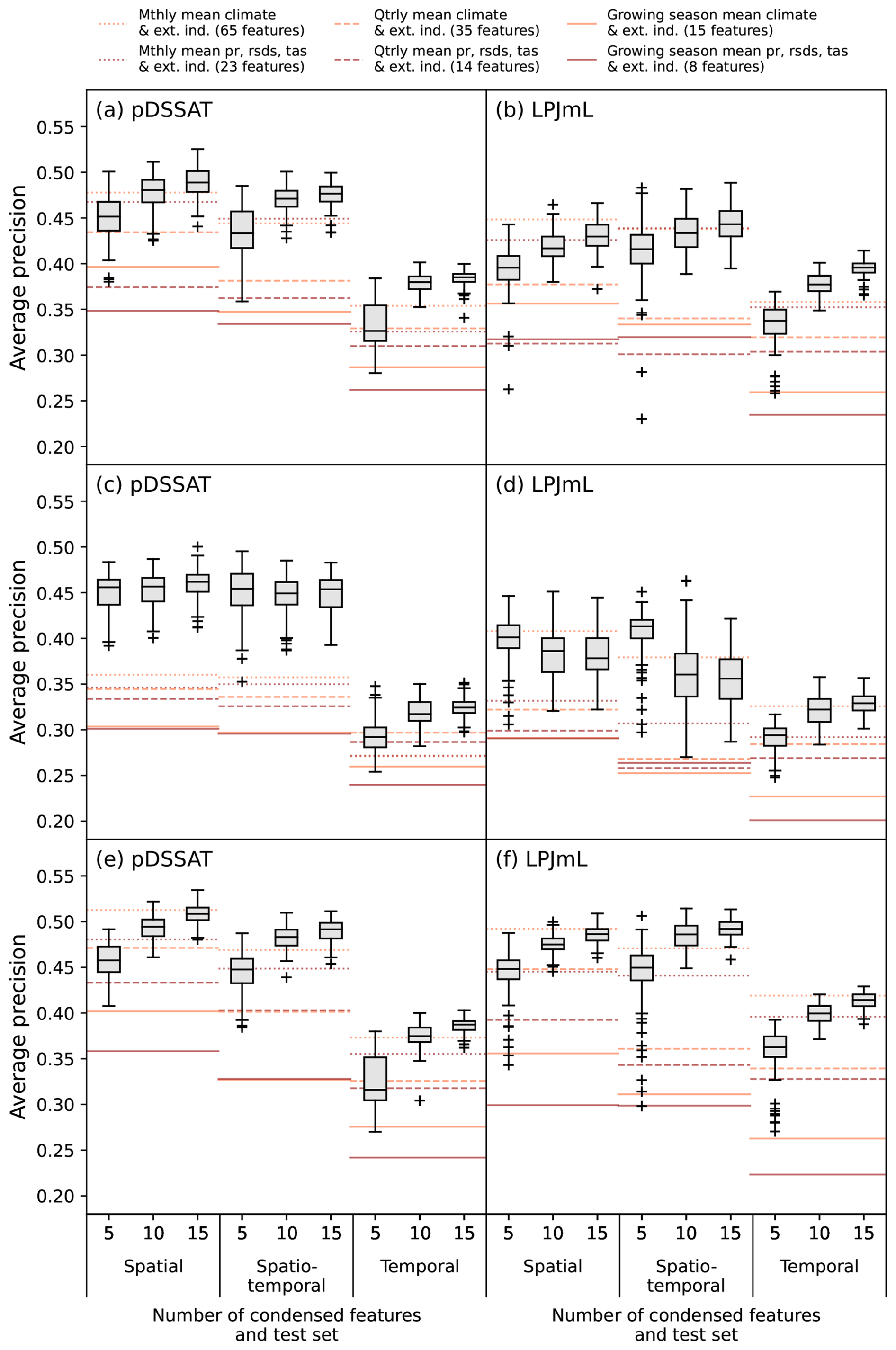
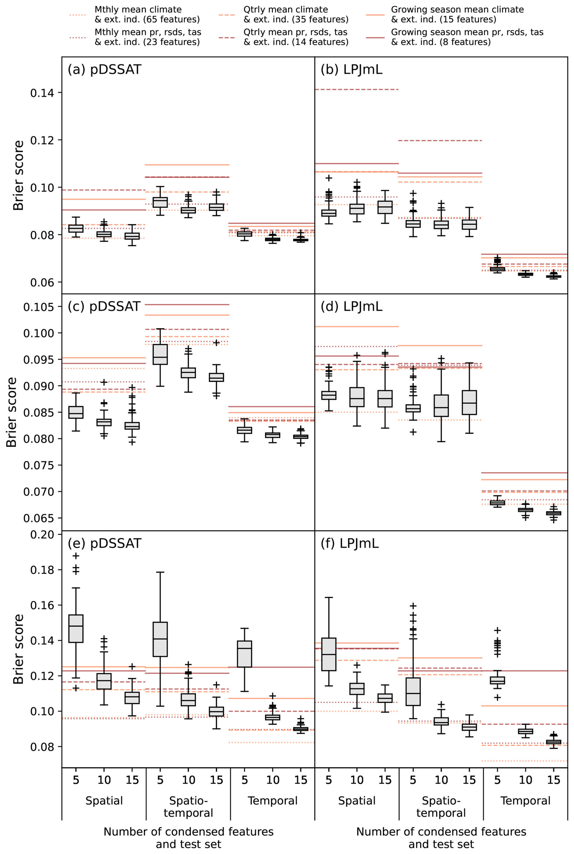
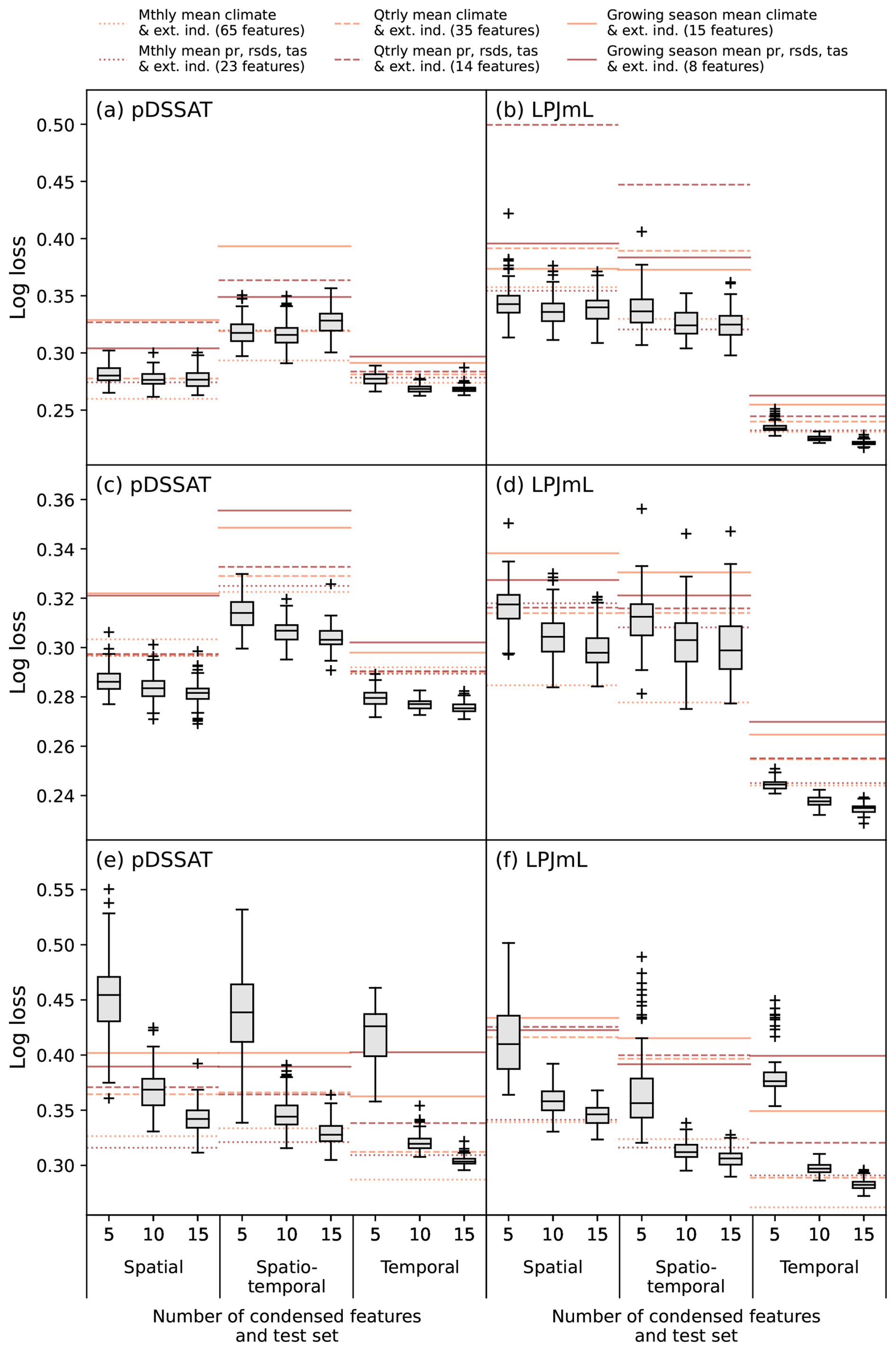
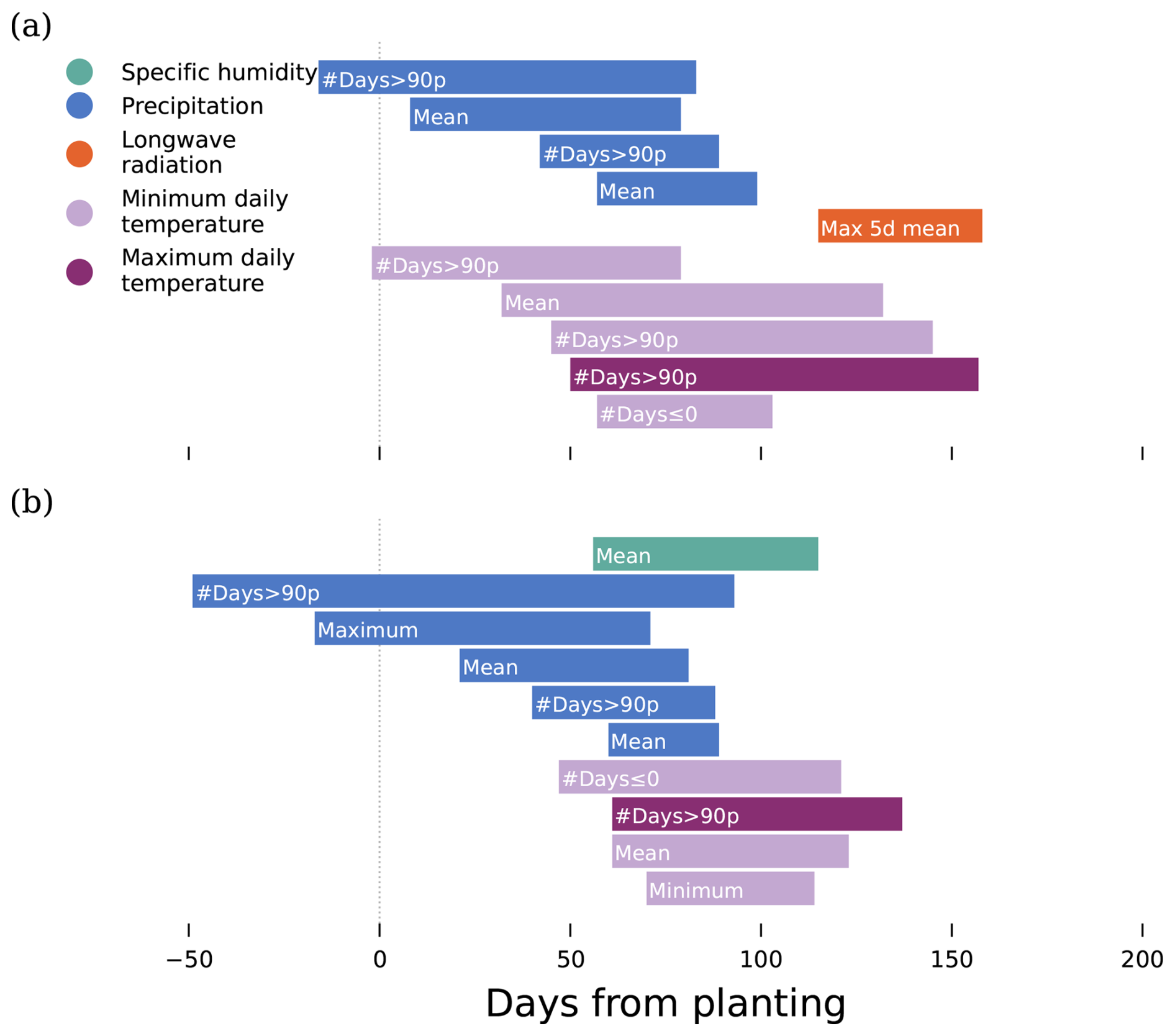
Figure C1 As Fig. 5, when yield failure is defined based on a 5th percentile threshold over the training years.

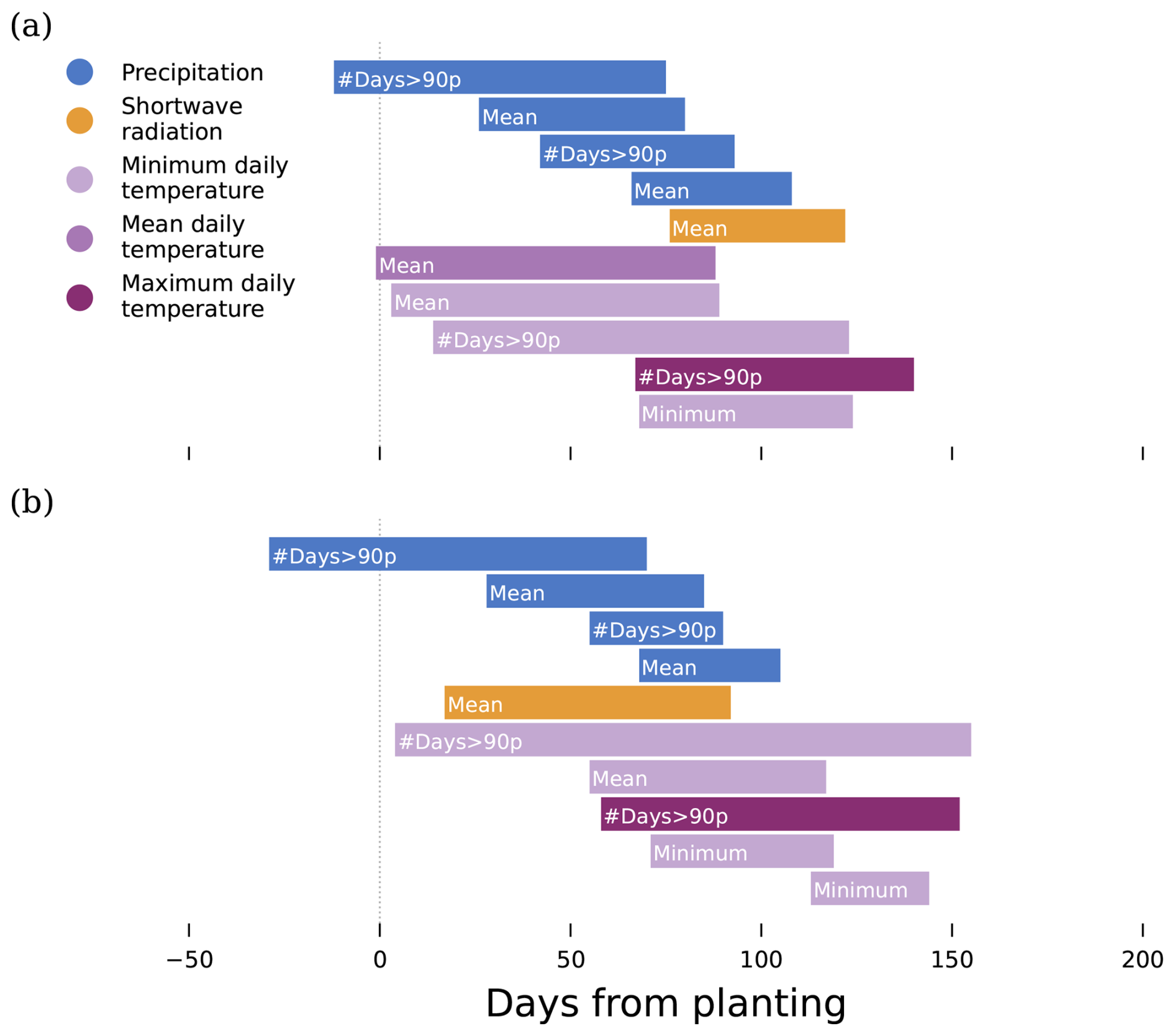
Figure C2 As Fig. 5, when yield failure is defined based on a 15th percentile threshold over the training years.

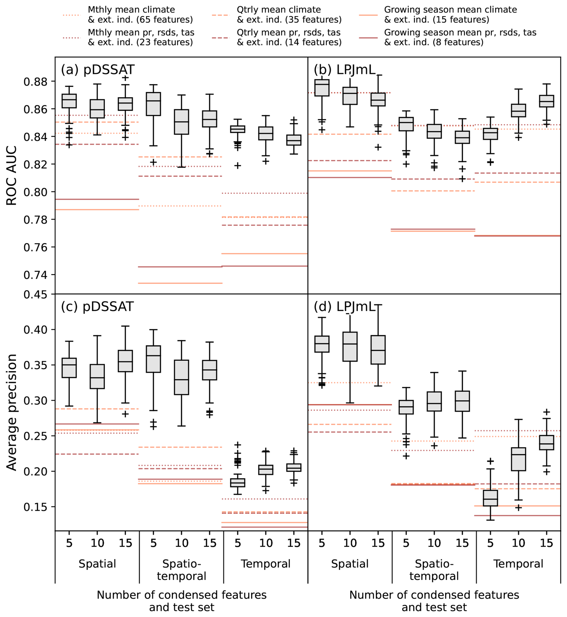
Figure C3 As Fig. 7, when yield failure is defined based on a 5th percentile threshold over the training years.

Figure C4 As Fig. 7, when yield failure is defined based on a 15th percentile threshold over the training years.

Appendix D: Sensitivity tests using different cross-validation strategies

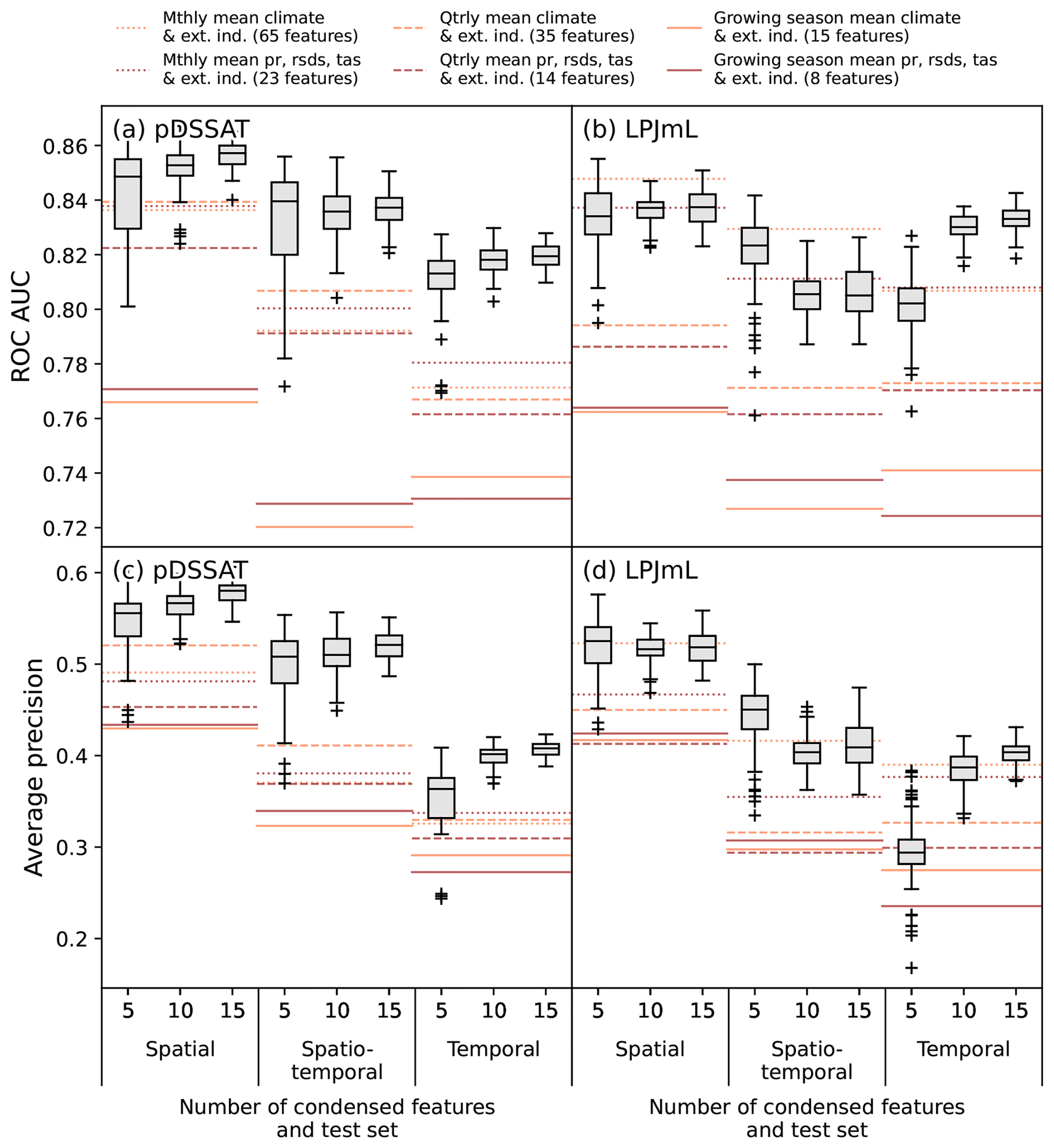
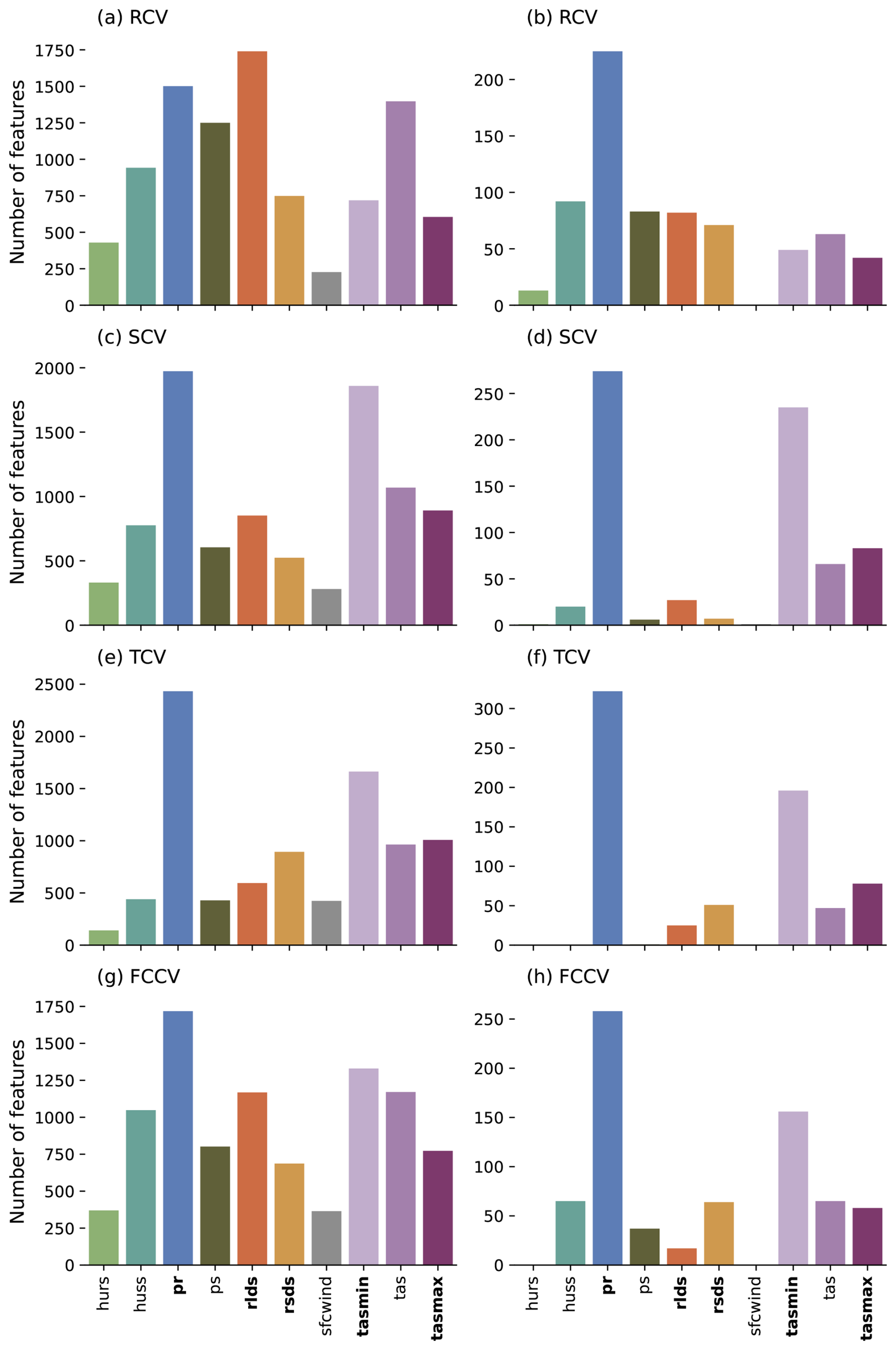
Figure D1 Climate variables used by features selected in Step 2 (a, c, e, g) and in drivers identified in Step 3 (b, d, f, h) for pDSSAT without detrending, depending on cross-validation strategy used to select features: random (RCV), spatial clusters (SCV), temporal (TCV) and feature-based clusters (FCCV). An exhaustive grid parameter sweep is performed (sampling 10, 20 or 30 time intervals in each pool; selecting 10, 20 or 30 features from each pool; and using 5, 10 or 15 cross-validation folds), using 20 pools per unique parameter combination, and sets of 5, 10 and 15 drivers are extracted. Features and drivers resulting from all parameter combinations are grouped by variable and counted.

Figure D2 As in Fig. D1, but for LPJmL without detrending.

Figure D3 As in Fig. D1, but for pDSSAT with yields detrended.

Figure D4 As in Fig. D1, but for LPJmL with yields detrended.

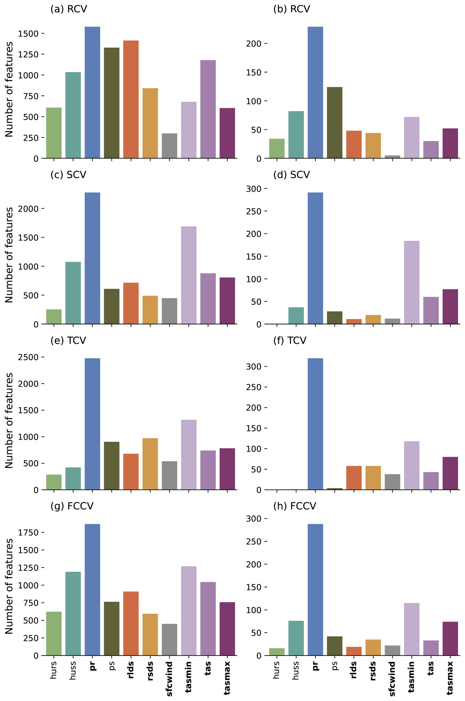
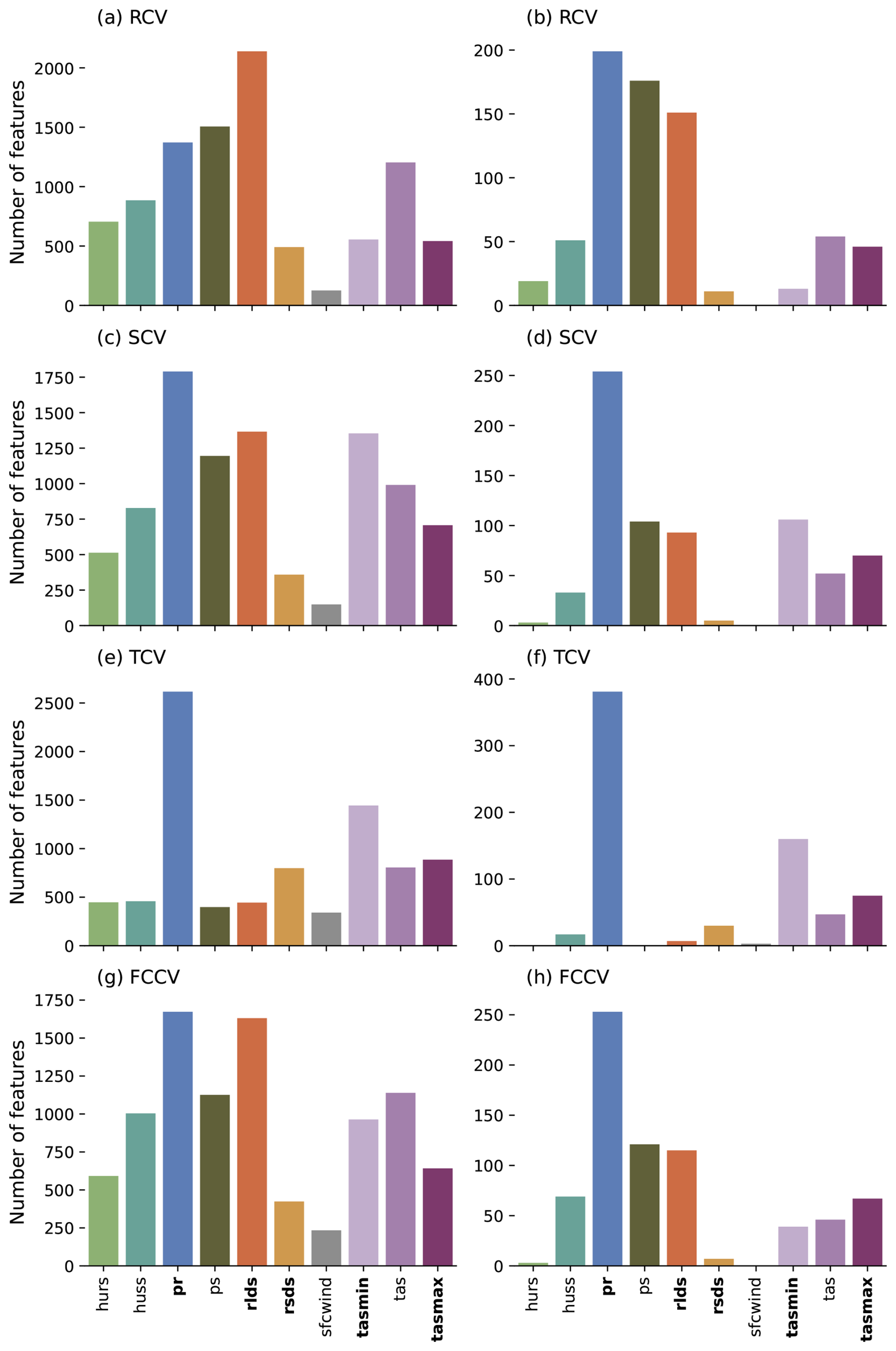
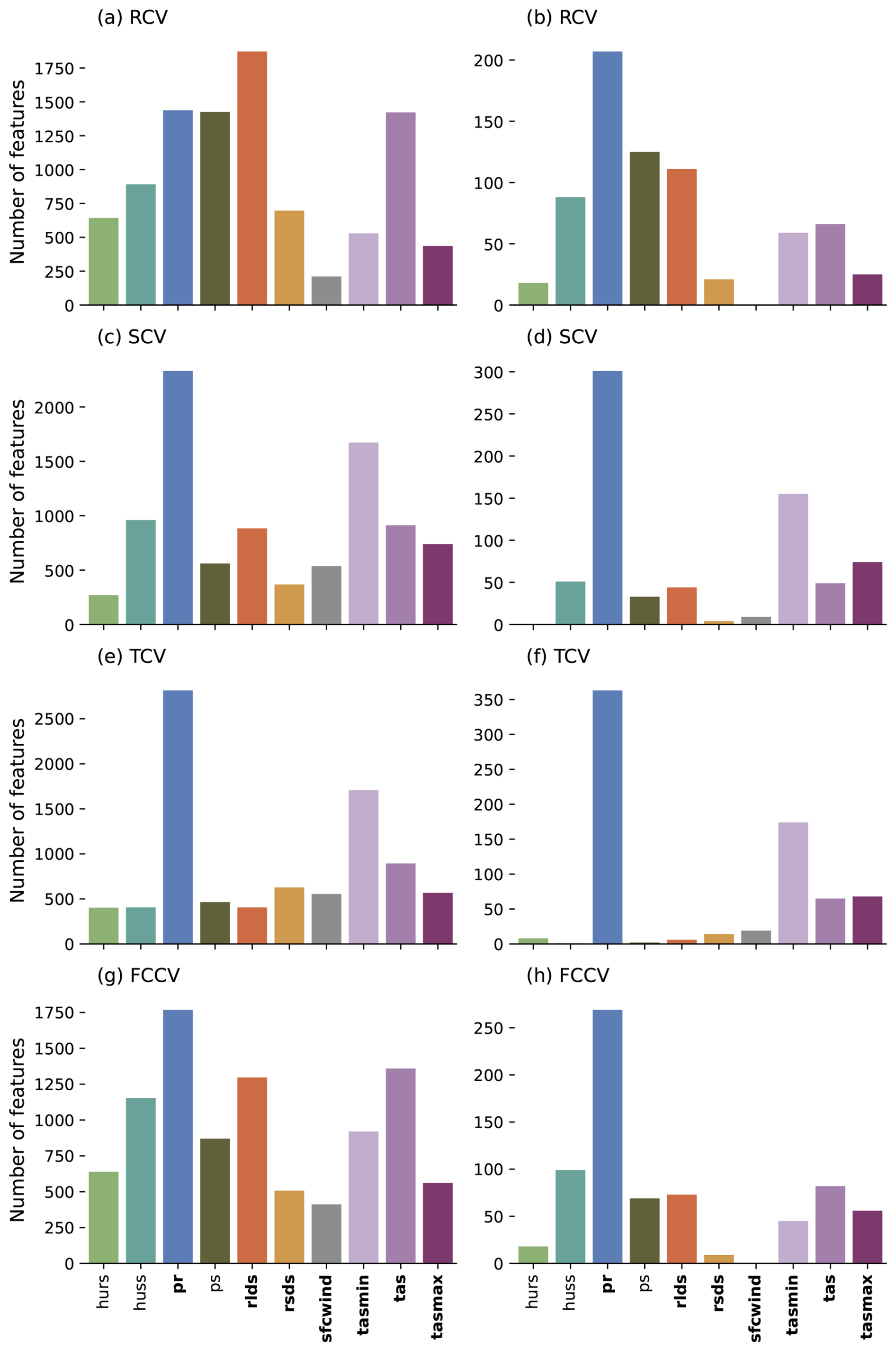
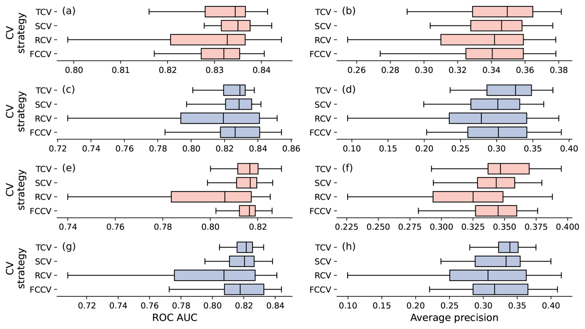
Figure D5 Performance on the test years of Lasso logistic regression models using identified driver sets as predictors, using different cross-validation strategies, based on the parameter sweeps described in Fig. D1. Panels (a), (b) show results for non-detrended pDSSAT (red); panels (c), (d) show non-detrended LPJmL (blue); panels (e), (f) show detrended pDSSAT (red) and panels (g), (h) show results for detrended LPJmL (blue).