Modeling PFAS in the global atmosphere – the PRIEST extension for the ICON-ART modeling framework

This study presents the ICON-ART (ICOsahedral Non-hydrostatic model framework with Aerosol and Reactive Tracers) PRIEST (PFCA Reactions In Earth System Transport) model extension, developed to simulate the transport and transformation of Per- and Polyfluorinated Substances (PFAS) in the atmosphere. While the ICON-ART framework was developed to simulate atmospheric physics and chemical composition, the newly developed PRIEST extension incorporates additional gas‐phase and aqueous physics, along with chemical reaction mechanisms, to model the transport, transformation, and deposition of Perfluoroalkyl Carboxylic Acids (PFCA) precursors. Therefore, the model includes 22 aqueous-phase reactions that depend on liquid cloud water and temperature. The aqueous-phase processes represent the adsorption of precursors in water droplets, with variable absorption rates. The model follows a hierarchical initialization, starting with the emissions, followed by aerosols, chemistry, and finally removal. To efficiently represent the atmospheric oxidative environment, PFAS chemistry is implemented in a semi-offline framework forced by prescribed monthly mean oxidant fields from CAM-chem. A simple parameterization of the OH radical is implemented to improve the simulation of PFCA precursors. The global model results (≈ 105 km² grid resolution and 6 h temporal resolution) show the capability of the model system to simulate regional and global variations of PFCA concentrations and their deposition processes. The results reveal an overestimation of atmospheric concentrations observed in Europe and an underestimation in East Asia. These differences are mainly related to the coarse spatial model resolution and the uncertainties arising from the underlying emissions model. In conclusion, ICON-ART PRIEST represents a significant step forward in simulating the atmospheric fate of PFCAs precursors and their transformation products by integrating an enhanced chemical mechanism into the ICON-ART framework that couples both gas-phase and aqueous-phase processes, and also with the incorporation of a detailed temporally resolved PFAS emission inventory.

1 Introduction

Per- and Polyfluorinated Substances (PFAS) are posing environmental challenges due to their ability to travel great distances from their primary sources (industrial production, disposal of everyday use products, and airports' firefighting exercises). PFAS have a long persistence in the environment and pose a threat to human health and the environment (Armitage et al., 2006; Prevedouros et al., 2006; Buck et al., 2011; Evich et al., 2022). PFAS constitute a vast and complex group ranging from 8000 to approximately 7 million different chemical compounds (Schymanski et al., 2023). It is important to note that within this family of compounds, not all exhibit identical properties or similar behaviors in the environment, but within this diverse group of substances, there are several subclasses. These include the Perfluoroalkyl Carboxylic Acids (PFCAs) where the compounds with eight or more perfluorinated carbon atom chains are defined as Long-Chain perfluorocarboxylic acids (LC-PFCAs), such as perfluorooctanoic acid (PFOA) and perfluorononanoic acid (PFNA). These compounds (as well as other long-chain PFAS) have raised interest due to three fundamental characteristics that make them especially concerning: their long lifetime, their capacity for bioaccumulation in living organisms, and their documented toxicity, so classified into the Persistent, Bioaccumulative, and Toxic group substances (PBT) (Stockholm Convention on Persistent Organic Pollutants, 2022; Buck et al., 2011). The potentially harmful effects of these substances on human health have been the subject of several studies (Wang et al., 2016; Rand and Mabury, 2017; Longpré et al., 2020; Zango et al., 2023; Coperchini et al., 2024). Thus, their extended fluorinated chain increases chemical stability and resistance to degradation but also enhances the compounds' capacity for bioaccumulation and long-range transport (Prevedouros et al., 2006; Buck et al., 2011; Environment and Climate Change Canada, 2023). The rise in industrial production of synthetic chemical compounds for everyday products has increased environmental burden and human exposure to PFCAs (Sunderland et al., 2019; Silva et al., 2021; Wang et al., 2015; Cserbik et al., 2023).

Identifying key sources, pathways, and sinks of PFCAs is crucial for estimating their adverse effects on human health (Sunderland et al., 2019; Wang et al., 2014). This understanding is particularly important within the framework of planetary boundaries, where PFAS (including PFCAs) are considered “Novel Entities” (Richardson et al., 2023).

Besides direct emissions of PFCA compounds, these may also be the result of a transformation of volatile precursor compounds into PFCAs through chemical reactions. Understanding the atmospheric oxidation, chemical degradation, interactions like aqueous phase, and physical removal mechanisms as deposition is essential for comprehending their environmental impact. Precursor compounds (see Table A1 in Appendix A) such as Fluoro Telomer Alcohols (FTOHs), Fluoro Telomer Olefins (FTOs), and Fluoro Telomer Iodides (FTIs) interact with other compounds like hydroxyl radicals (OH), peroxy (RO₂), and hydroperoxy (HO₂) radicals, which are photochemically formed and generate a relatively slow oxidation process (leading to a FTOH 68 % to >98 % consumption in 0.5 to 15 min) (Ellis et al., 2004; Stockholm Convention on Persistent Organic Pollutants, 2022). They also react with abundant substances, including nitrogen monoxide (NO), nitrogen dioxide (NO₂), and water vapor (H₂O). This leads to complex interactions that produce intermediate species and ultimately (after 10 to 20 d), highly persistent long chained Perfluorinated Carboxylic Acids (LC-PFCAs) (Young and Mabury, 2010; Wallington et al., 2006).

Efforts to implement policies to reduce the use and the emissions of PFAS (PFCAs included) have primarily targeted long-chain compounds (C8+), while legislation for precursors has been overlooked. Consequently, emissions of these precursors have not decreased since the early 1970s (Prevedouros et al., 2006) but continue to rise until today, contributing to an increase in the global PFCAs budget between 10 % and 30 % (Wallington et al., 2006; Yarwood et al., 2007; Thackray et al., 2020). A table with a wider PFAS speciation (Including PFCAs and FTOH precursors) is included in the Table A1.

Meteorological conditions and their evolution strongly influence the atmospheric transport, transformation, and deposition of PFCAs and their precursors. Seasonal changes in temperature and sunlight intensity influence the photochemical reactions that convert volatile precursors into stable PFCAs, while variations in wind speed and direction modulates how these compounds are dispersed over local and global scales. Moreover, precipitation patterns and humidity (often dependent on latitude and proximity to large water bodies, such as the global oceans) influence the most efficient removal mechanisms of PFCAs through wet deposition (Thackray and Selin, 2017; Thackray et al., 2020).

To address these complex interactions, we developed PRIEST, an extension to the ART component implemented in the ICON model framework. ICON-ART PRIEST introduces aqueous-phase chemistry to simulate the adsorption and partial dissolution of gaseous-phase compounds in atmospheric water droplets (following Henry's Law). These compounds are redistributed as aerosols, leading to subsequent wet deposition. This extension improves the representation of PFCA precursors' transformation, transport, and scavenging within the atmosphere building upon other authors previous modeling efforts (Thackray and Selin, 2017; Thackray et al., 2020; Wallington et al., 2006). ICON-ART PRIEST also improves the spatial resolution to approximately 105 km², finer than previous global efforts using 4 × 5°. We integrate an up-to-date, temporally and spatially resolved emission model (POPE) which includes PFCAs and precursors considering different compartments including industrial production, consumer product usage and disposal, and airport firefighting exercises. Additionally, POPE accounts for emissions to water bodies and incorporates air-water partitioning. Previous studies have emphasized the importance of atmospheric precursors in establishing the global burden of these compounds (Wallington et al., 2006; Yarwood et al., 2007; Thackray et al., 2020). In this regard, emissions of 8 : 2 fluorotelomer olefin (8 : 2 FTO) and 8 : 2 fluorotelomer iodide (8 : 2 FTI) are derived from 8 : 2 fluorotelomer alcohol (8 : 2 FTOH) emissions according to the criteria established by Thackray et al. (2020). Specifically, 48 % of the total emissions are attributed to 8 : 2 FTOH, an equal fraction to 8 : 2 FTO, and 4 % to 8 : 2 FTI, based on Wang et al. (2014); Prevedouros et al. (2006). Emissions are also included for PFOA and PFNA (the primary PFCA products) instead of only for the precursor compounds (Wallington et al., 2006), which allows us to calculate the total burden of these compounds from emissions and releases.

PRIEST's gas-phase reaction mechanism is based on Thackray et al. (2020) but is further extended with 22 aqueous-phase reactions (Table B3 in Appendix B), and adopts a fully online-coupled approach that simultaneously resolves meteorology and global-scale chemistry.

Through the evaluation of ICON-ART PRIEST, we examine how the simulations adjust with observed atmospheric concentrations and wet deposition patterns across different regions, helping identify potential sources of uncertainty and areas for future improvement.

2 Model description

This section introduces the PRIEST extension of the ART (Rieger et al., 2015; Weimer et al., 2017; Schröter et al., 2018) component in the ICON framework (Zängl et al., 2015) in more detail. The objective of PRIEST is to extend the ICON-ART framework by integrating a detailed representation of the chemical transformation processes (oxidation and photochemical degradation) that convert atmospheric precursors into PFCA while simulating the long-range transport, deposition, and ultimate environmental fate of these persistent compounds. This would allow us to predict their global distribution and set a basis to assess their potential risks for ecosystems and human health.

2.1 Overview of ICON-ART

The ICON modeling framework (Zängl et al., 2015) is a next-generation atmospheric circulation model with an integrated ART sub-module (Rieger et al., 2015; Schröter et al., 2018; Weimer et al., 2017). ICON can accurately represent atmospheric physics and composition solving the primitive equations on an icosahedral-triangular Arakawa C grid (unstructured), enabling multi-scale simulations. ART complements this by reproducing gas-phase chemistry and aerosol dynamics transport from emission sources. As a flexible framework, ICON-ART can perform both limited area and global simulations with nesting in specific zones.

The ART module on its own is in charge of the aerosols, gas-phase, and heterogeneous chemistry in the global model. Tracers in ICON-ART are transported following the continuity equation of mass (Miura, 2007; Lauritzen et al., 2011; Rieger et al., 2015; Weimer et al., 2017). In this case, our ICON-ART tracers utilized are 31 gas-phase species and 14 aqueous species including the external reactant inputs (further described in Sect. 2.2.1), intermediate products, precursors (8 : 2-FTOH, 8 : 2-FTO and 8 : 2-FTI), and PFCAs final products (such as PFOA and PFNA).

ICON-ART uses Smooth Level Vertical (SLEVE) coordinates to avoid the numerical errors and instability produced by the then commonly used terrain-following coordinates. The coordinates apply a smoothing function to the terrain by increasing the decay rate of the coordinate surfaces. This creates a progressive transition from the levels that closely follow the terrain near the surface to smoother levels in the free troposphere, allowing smaller-scale terrain features to be removed more efficiently with height (Schär et al., 2002; Leuenberger et al., 2010; Prill et al., 2024).

2.2 Implementing ICON-ART PRIEST

To study PFCAs, we introduced and updated several mechanisms in the ICON-ART framework, leading to the ICON-ART PRIEST extension. The ICON-ART full chemistry routine was enhanced and linked to the gas-aerosol interactions to enable PFCA simulations. The key focus was extending the simplified gas-phase reaction mechanism (Tables B1 and B2) from fluorotelomer precursors to PFCAs (Thackray et al., 2020). This is achieved by implementing both gas-phase reaction mechanisms and aqueous-phase chemistry (Table B3), which are crucial for a more physically accurate simulation of the fate of fluorotelomer PFCA precursor and their products (due to their solubility into water) in the atmosphere and their deposition. Furthermore, the model was improved to account for diurnal variations in OH radical production, addressing the rapid reaction rates induced by ultraviolet radiation and avoiding the overestimation of PFCA production. These developments contribute to a more comprehensive representation of PFCAs atmospheric transport and sinks using the ICON-ART modeling framework.

2.2.1 Gas-phase reaction mechanism

To study PFCAs in ICON-ART, we integrated aqueous-phase chemistry (Table B3) into ICON-ART based on the simplified gas-phase (Tables B1 and B2) PFCAs reaction mechanism built by Thackray et al. (2020). Originally, the mechanism accounted for 31 gas-phase and two photolytic reactions. It calculates the degradation of 8 : 2 FTOH, 8 : 2 FTO, and 8 : 2 FTI (where 8 : 2 represents the 8 fluorinated carbons, and a 2 carbon ethyl alcohol group in the molecule) as the main commonly emitted fluorotelomer PFCAs precursors (Prevedouros et al., 2006; Wang et al., 2014). The mechanism addresses the fluorotelomer dissociation to form FT-aldehyde, which can be oxidized or photolyzed to form peroxyl and acyl-peroxy radicals, which can react with NO, NO₂, RO₂, HO₂, and H₂O to form intermediate products and react again with OH or ultraviolet radiation to produce PFOA and other PFCAs (Thackray and Selin, 2017; Thackray et al., 2020). The reactants involved in the reaction mechanism are initialized based on atmospheric concentrations provided by CAM-chem (Emmons et al., 2020), which are provided as monthly means for all reactants except OH.

Aqueous phase interactions are crucial to simulate PFCAs reactions, transformation and transport due to the solubility of anionic PFCAs into water, such as PFOA and PFNA (Prevedouros et al., 2006; Young and Mabury, 2010). To simulate the gas dissolution into water droplets, we incorporated an additional set of 22 aqueous reactions to extend this mechanism (Table B3). These reactions consider the Liquid Water Content (LWC) from liquid cloud droplets and temperature. After adsorption, gas-to-water droplet dissolution is treated as mixed aerosols in the accumulation and coarse modes into the ART aerosol dynamics sub-module (further described in Fig. 1). Doing this, a better representation of the PFCAs environmental behavior is possible.

Figure 1 Flowchart showing the implemented chemistry processes for PFCA species and precursors in ICON-ART PRIEST. The parts marked in yellow correspond to the processes added to the complete chemistry module to extend ICON-ART.

The adapted and improved gas-phase chemistry mechanism has been incorporated into ART using the Module Efficiently Calculating the Chemistry of the Atmosphere (MECCA), an external module developed by Sander et al. (2019). MECCA is a Kinetic Pre-Processor (KPP) based module (Damian et al., 2002) that solves chemical kinetics through a non-linear system of ordinary differential equations derived for a given chemical mechanism.

To account for OH concentrations which depend on solar radiation, we redistributed the monthly OH fields from CAM-chem (See Sect. 3.1.1) as a function of incoming radiation patterns. Therefore, if the “shortwave net flux at surface” (swflxsfc) value is 0 in any grid cell, the OH value will become 0 in that cell. Contrarily, if radiation exceeds a maximum radiation threshold of 1000 W m⁻² the OH will take the maximum value calculated from the six hourly data along the respective month for that cell. For all other grid cells, OH concentrations depend on the specific cell's OH normalization respecting radiation relative to the maximum radiation threshold.

The maximum global solar irradiance threshold is defined as the truncated mean of the extraterrestrial solar constant (1368 W m⁻²) reduced by the Earth's planetary albedo (≈ 0.31), yielding ≈ 944 W m⁻² at surface level. This formulation builds on foundational theoretical estimates of the solar constant and albedo balance, early applied solar models, surface and satellite-based observations (Zdunkowski et al., 2007; John and William, 1991; Urraca et al., 2017).

This is necessary because OH radicals are rapidly formed when ultraviolet radiation is present. Using monthly averaged values would neglect the effect of the diurnal cycle and its impact on OH production, especially during the night, when it is barely produced. Neglecting the diurnal effect could potentially generate an OH overproduction, which in turn can affect the PFCAs production.

While we acknowledge that this offline approach simplifies the instantaneous covariance between OH and short-lived drivers like NO_x, it provides a computationally efficient approximation of the atmosphere's oxidative capacity. Given that PFCA precursors (e.g., 8 : 2 FTOH, 8 : 2 FTO, and 8 : 2 FTI) have atmospheric lifetimes on the order of weeks (Young and Mabury, 2010; Thackray et al., 2020; Wallington et al., 2006), their transport is driven by integrated OH exposure rather than rapid chemical fluctuations. Therefore, scaling monthly climatological fields by instantaneous solar radiation preserves the necessary diurnal bounds without mandatorily requiring a fully coupled online chemistry scheme.

In ICON-ART PRIEST, reactants from CAM-chem (NO_x, OH, RO₂, HO₂, and H₂O) are not transported as prognostic tracers. They are ingested only as prescribed monthly-mean background fields to compute PFAS reaction rates. The only species that are prognostically transported and deposited by ICON-ART PRIEST are the PFCA tracers (e.g. PFOA, PFNA, 8 : 2-FTOH) and the associated mixed aerosols, together with the meteorological state. Consequently, the CAM-chem-derived species have no continuity or momentum equations in ICON; there is no second dynamical core, and the conservation equations for mass and momentum solved by ICON remain unaltered. Because the CAM-chem fields are used in monthly-mean form, most sub-monthly dynamical variability associated with transport is already filtered out, so they act as slowly varying climatological oxidant fields, consistent with standard semi-offline couplings widely used in regional and global chemistry–transport modeling.

2.2.2 Aqueous phase reaction mechanism

Due to the high solubility of long-chain, highly fluorinated substances, it is necessary to implement aqueous‐phase processes in the model. Initially, emissions of PFCA precursors are configured by reading metadata (provided by the user into an emission XML file declared in the namelist file; this XML provides the variable name, dates, and path to the files into the POPE files remapped to ICON-ART containing directory (Weimer et al., 2017). Next, relevant reactants (e.g., H₂O, NO, NO₂, OH, and HO₂) are read as monthly values from CAM-chem fields to prepare the gas-phase reaction mechanism.

Once the gas-phase chemistry is ongoing, the model activates aqueous-phase reactions, the model calculates the water mass (addition of water mass into aerosol modes droplets) into a droplet and H₂O fraction in aerosols. These calculations provide a basis for the calculation of detailed aerosol properties, the liquid water content (LWC) volume ratio, and droplet characteristics, such as diameter, surface ratio, and equivalent radius (calculated from diameter and surface ratio). Next, aqueous tracers from aerosols are calculated and sent to the intermediate linking interface init_aero_chem_matrix to then simulate the adsorption and dissolution of gaseous PFCA precursors (and their products) to partition onto aerosol. These aqueous tracers (aerosol tracers with dissolved PFCAs), once formed, are subject to wet deposition, facilitating their atmospheric removal through grid-scale, convective, and scavenging processes (Fig. 1).

The dissolution of PFCAs gas into water droplets is a dynamic and complex process. When these compounds interact with atmospheric water droplets (cloud, fog, aerosol liquid water, etc.), they can transition from the gas-phase to the aqueous-phase. At this point, two processes occur: adsorption (where gas-phase molecules attach to the droplet surface) and dissolution, driven by Henry's law, which describes the equilibrium partitioning between gaseous species and liquid water. Thus, a compound with a high Henry's constant favors the air, while a low value indicates it readily dissolves in water; however, it does not consider the timescale over which equilibrium is achieved. To address this limitation, the model introduces a time-dependent absorption rate that relies on several kinetic factors: gas-phase diffusion, transfer across the gas–water interface, diffusion within the aqueous phase, and any reactions in solution (Steinfeld, 1998; Bruckert, 2023; Schwartz, 1986). This approach ensures that highly soluble species, such as PFCAs (and their precursor products), are modeled more realistically than would be possible with a simple instantaneous equilibrium assumption.

Anionic PFCAs (like PFOA and PFNA) are characterized by low vapor pressure, low Henry's constant, and high water solubility, making them the dominant species in particulate matter, where they have been found sorbed to atmospheric particles (aerosol droplets) (Sosnowska et al., 2023). When gas-phase PFCAs dissolve into water droplets, this process is known as aqueous-phase secondary organic aerosol formation (aqSOA). As a result, the droplets become PFCA-containing aerosols. The most common particle-phase PFCAs, such as PFOA and PFNA, have a diameter of about 0.3 µm and between 0.1 to 1 µm, respectively (Faust, 2022).

Within ICON-ART, aerosol dynamics include ten log-normal distributions that account for Aitken, accumulation, and coarse particles across several modes, including soluble, insoluble, and mixed states, as well as an additional giant insoluble mode.

To represent the aqueous-phase secondary organic aerosol (aqSOA) formation process and dissolution products, we use the mixed modes included in ICON-ART for the Accumulation and Coarse modes based on PFOA and PFNA particle sizes. This means PFCA species, once dissolved into water, partition into these two aerosol categories rather than remaining in the gas phase. The reasoning is that anionic PFCAs are highly water-soluble, so they readily dissolve into liquid water present in aerosols or cloud droplets. In the model, gas-phase PFCAs can adsorb onto existing aerosol particles and dissolve into the corresponding particle's aqueous phase. This effectively creates PFCA-enriched droplets or “coated” aerosols in the accumulation and coarse size ranges. The partitioning is implemented such that during each chemistry timestep, if conditions are favorable, gaseous PFCA precursors/products transfer into the corresponding mixed aerosol reservoirs (accumulation or coarse). The “mixed acc” aerosol represents smaller aqueous particles taking up PFCAs, while “mixed coa” aerosol represents larger particles. By classifying PFCAs into these mixed aerosol modes, the model captures how PFCAs dissolve into water-containing particles rather than remaining as purely dry aerosols or unattached gas.

The subroutine init_aero_chem_matrix plays a key role as the intermediate interface between the aqueous-phase tracers and the redistribution in their respective aerosol modes. Following this, the model redistributes the aqueous tracers to the aerosol modes. This redistribution reflects the formation of core-shell mixed aerosols, where the dissolved species are partitioned between the accumulation and coarse modes according to the LWC and the radius a droplet would have with that given LWC. In Fig. 1, the init_aero_chem_matrix is an intermediate process implemented within the full chemistry routine, and the matrix is being written at the time when the calculations from the chemistry solver are completed per timestep.

3 Model setup

To run the ICON-ART PRIEST, the Starter Package for ICON-CLM Experiments (SPICE) runtime environment (Rockel and Geyer, 2022) is used. SPICE is a collection of scripts developed by the Climate Limited-area Modelling Community (CLM) to efficiently perform ICON experiments. SPICE takes care of the initial and boundary conditions of meteorological preprocessing preparing it to be initialized in the ICON Icosahedral grid. It is also very efficient in scheduling jobs for long-term simulations on High Performance Clusters (HPCs). For this study, to evaluate the ICON-ART PRIEST modeling results for PFCA concentrations and depositions we adapted SPICE for a global grid setup and incorporated the atmospheric chemistry options into the namelist execution files.

In this study, we use an icosahedral R03B04 global grid (46 080 cells), where the first number represents the root division and the second represents the bisections (Weimer et al., 2017), here the spatial grid resolution is approximately 105 km².

The ICON-ART PRIEST model was run for the period from January 2000 to July 2019, focusing on the eight-carbon chain reaction mechanism. This produced PFOA and PFNA as final products, along with several intermediate products such as Peroxyl radicals (e.g. FTOO82, PFOO8, PFOO7, FPER81 and FPER82 in Table B1). Simulated concentrations and deposition of PFCAs were compared with measurements to evaluate the model's capabilities to simulate PFCAs globally.

We apply a recently developed emission inventory (Simon et al., 2024) for four groups of PFAS (PFCAs, PFSAs, FTOHs, and PFECAs) with 22 species, including different chain-lengths (Table A1), that are globally distributed on a 0.5° grid for each year from 1950 till 2020. Note that only the compounds marked with an asterisk in Table A1 are used for this study. To derive monthly emission rates for each grid point, a linear interpolation was done between the annual values of the preceding and following years for every grid point. Then emissions are adjusted gradually from one year to the next, eliminating the need for constant monthly rates and preventing abrupt changes during the December-to-January transition, while total annual emissions remain unchanged because the sum of the monthly emissions matches the assigned annual total. This provides a more homogeneous temporal emission distribution throughout the year. Emissions were also spatially interpolated to the ICON R03B04 grid (approximately 105 km²) for input into ICON-ART PRIEST. Then, emissions are provided in monthly emission rates.

3.1 Meteorological forcing

The simulation of meteorological fields in ICON runs with initial conditions forced by the ERA-Interim reanalysis (Dee et al., 2011) and remains unforced by further observations along the run-time period, meaning no data assimilation is applied. The simulation starts at 1 January of the year 2000. The original vertical levels are interpolated in 60 levels at the SLEVE coordinates (Schär et al., 2002; Leuenberger et al., 2010) used by ICON reaching a model top of 24 km distributed homogeneously in layers of 400 m. Since our study focuses primarily on the long range transport, the finer scale processes in the boundary layer or lower levels are less critical for our objectives. Consequently, we adopt a uniform vertical distribution to simplify the modeling setup without compromising the ability to capture the relevant large-scale characteristics like the synoptic and global transport. The model output is extracted every six hours and interpolated onto a 1° × 1° regular latitude–longitude grid. The total study period extends from 2000 to 2019, with monthly simulations for more efficient output processing; the first five years are treated as spin-up.

3.1.1 CAM-chem initial and boundary conditions

The initialization and boundary conditions for the reaction mechanism require the concentrations of involved reactants (NO, NO₂, HO₂, H₂O, OH, and RO₂). For this purpose, data from the Community Atmospheric Model with Chemistry (CAM-chem) was obtained (https://rda.ucar.edu/datasets/ds313.7, last access: 12 December 2025) (Lamarque et al., 2012; Tilmes et al., 2015; Emmons et al., 2020). This data is provided by the National Center for Atmospheric Research (NCAR) in the USA as part of the Community Earth System Model (CESM) ensemble (Kay et al., 2015).

CAM-chem is utilized in CESM to simulate Earth's atmospheric composition, incorporating the Model of Ozone and Related chemical Tracers (MOZART-T1) reaction mechanism, which accounts for 151 gas-phase species, 65 photolysis, and 287 kinetic reactions. From this database, six-hourly NO, NO₂, HO₂, H₂O, and OH values were extracted for the years 2001 to 2020 (the year 2000 is not available, so 2001 is used as analog), and then monthly averages were calculated. However, only for OH, the monthly maximum was computed (and provided as an input for the OH parameterization, described in Sect. 2.2.1), as the model is executed in monthly time intervals, and boundary conditions are provided for each restart for the chemical reactants.

The need for monthly initial conditions for H₂O from CAM-chem in ICON-ART, similar to the treatment of chemical species with less temporal variability, is mainly justified by the use of CAM-chem as a consistent source to initialize the complete state of the atmosphere. Additionally, H₂O plays a key role in multiple reactions of the chemical mechanism, including the formation of the hydroxyl radical (OH). Since the initial chemical concentrations come from an external model (CAM-chem), it is essential to maintain consistency between the reactive species that condition their reaction rates. The inclusion of H₂O from the same source as the chemical species ensures a reliable representation of the atmospheric chemical state at the time of initialization, minimizing mismatches that could compromise the realistic evolution of chemistry in the early stages of the simulation. While atmospheric humidity exhibits variations on much shorter timescales, the use of monthly H₂O data provides a consistent re-starting point, allowing ICON's own dynamics to rapidly adjust the H₂O field to synoptic timescales. This practice is common in atmospheric modeling studies focusing on long-term chemical evolution, where initial consistency between variables is essential.

To obtain the concentrations of the RO₂ radicals, calculations based on OH, HO₂, and three of the most abundant hydrocarbons in the atmosphere (CH₄, C₂H₆, C₃H₈) were used.

Organic Peroxyl Radicals are generally summarized as RO₂. In the gas-phase reaction mechanism, reactions with these radicals are key for understanding the PFCA production in remote regions, especially in those where NO concentrations are low (Young and Mabury, 2010). However, RO₂ is often not included as a product from atmospheric concentration databases or model products because its atmospheric lifetime is short and its chemistry highly reactive. Nevertheless, RO₂ is an essential reactant due to its interaction with many other compounds, and is particularly important in the degradation chain of PFCA precursors. In the present PRIEST version, RO₂ is therefore diagnosed following Thackray and Selin (2017) from reactions of OH with the three most abundant alkanes (CH₄, C₂H₆, C₃H₈) and subsequent loss via NO and HO₂ (Eq. 1):

$$\begin{array}{}\text{(1)}& \left[{\mathrm{RO}}_{\mathrm{2}}\right]\approx {\displaystyle \frac{\begin{array}{c}\left[{\mathrm{CH}}_{\mathrm{4}}\right]\left[\mathrm{OH}\right]k_{\left({\mathrm{CH}}_{\mathrm{4}}+\mathrm{OH}\right)}+\left[{\mathrm{C}}_{\mathrm{2}}{\mathrm{H}}_{\mathrm{6}}\right]\left[\mathrm{OH}\right]k_{\left({\mathrm{C}}_{\mathrm{2}}{\mathrm{H}}_{\mathrm{6}}+\mathrm{OH}\right)}\\ +\left[{\mathrm{C}}_{\mathrm{3}}{\mathrm{H}}_{\mathrm{8}}\right]\left[\mathrm{OH}\right]k_{\left({\mathrm{C}}_{\mathrm{3}}{\mathrm{H}}_{\mathrm{8}}+\mathrm{OH}\right)}\end{array}}{\left[\mathrm{NO}\right]k_{\left(\mathrm{NO}+{\mathrm{RO}}_{\mathrm{2}}\right)}+\left[{\mathrm{HO}}_{\mathrm{2}}\right]k_{\left({\mathrm{HO}}_{\mathrm{2}}+{\mathrm{RO}}_{\mathrm{2}}\right)}}}\end{array}$$

Then, calculated RO₂ from CAM-chem most abundant VOCs is prescribed as background fields. These fields are neither transported nor chemically updated within ICON and thus do not enter the internal mass budget of the transported PFAS tracers, as for the rest of the background concentration reactants. As a consequence, the approximate RO₂ diagnostic used here should not have a significant impact in the global mass conservation of PFCAs in PRIEST. Nevertheless, from a chemical-mechanism perspective, diagnosing RO₂ from a limited VOC subset and prescribed OH/HO₂/NO_x fields breaks the strict chemical coupling that would ideally link VOCs with this compounds.

The offline diagnostic of RO₂ limitation is acknowledged in the current PRIEST version, and it will be calculated following a fully online interactive approach in a future release. This will be achieved by incorporating the calculation into the gas-phase reaction mechanism (Sect. 2.2.1), so that RO₂ production and loss are fully consistent with the VOCs and oxidant fields.

3.1.2 The Persistent Organic Pollutants Emission model (POPE)

The Persistent Organic Pollutant Emissions (POPE) model and inventory aims to provide temporally and spatially resolved model-ready emissions for 23 of the most widely used Per-and Polyfluoroalkyl Substances (PFAS) including Perfluoroalkyl carboxylic acids, Perfluorosulfonic acids, Fluorotelomer alcohols, and novel replacements.

POPE covers the time span from the first industrial-scale production in 1950 up until 2020 annually on a grid with 0.5° resolution. Emissions into the air and emissions into water are treated separately (Simon et al., 2024). The POPE inventory is publicly available in GEIA's (Global Emission InitiAtive) ECCAD data portal: https://permalink.aeris-data.fr/POPE (last access: 20 July 2026).

The POPE model distributes estimated total PFAS emissions in space and time based on several data sets such as the European Pollutant Release and Transfer Register, the Nomenclature statistique des activités économiques dans la Communauté européenne and United States Environmental Protection Agencies Facility Registry Service in combination with socio-economic data such as population (Chambers, 2022) and Gross Domestic Product (GDP) (Kummu et al., 2018). This is complemented by estimates for individual point sources, industrial sites, and airports (Will et al., 2005; Dalmijn et al., 2024), whereby the source activity is dependent on regional changes in production volumes, usage quotas, and recapturing efficiency (Brennan et al., 2021; Paustenbach et al., 2007). Some regional emission data for water bodies (Pistocchi and Loos, 2009; Filipovic et al., 2015) or national level estimates (OECD, 2018) are also considered. POPE includes emissions by industrial production, diffuse emissions through usage and disposal of consumer products, secondary emissions from the reaction of precursors, and emissions by firefighting exercises on airports using Aqueous Film Forming Foams (AFFF).

The POPE emission inventory expands on previous global emission estimates for example by Wang et al. (2014) or Prevedouros et al. (2006). Furthermore POPE, in conjunction with a river transport model (Hagemann and Dümenil Gates, 2001), has been compared to independent measurements of PFAS river concentrations (Mclachlan et al., 2007; Heydebreck et al., 2015), with the majority being compatible with the estimated bounds (lower bound, best guess, and upper bound).

3.2 Observational datasets

To validate our chemical transport model results, we integrated observational datasets from multiple global monitoring databases as well as scientific publications. From the following datasets we assembled atmospheric concentration and wet deposition measurements, in a measurement database for different PFAS compounds:

• Atmospheric concentrations: Data was obtained from the Stockholm Convention's Global Monitoring Plan (GMP) Data Warehouse (DWH) (GMP DWH et al., 2020), the United Nations Environmental Programme (UNEP) (UNEP, 2024), the European Monitoring and Evaluation Programme (EMEP) database (EBAS), and Persistent Organic Pollutants Exp (PoPs EXPs) (Dong et al., 2021), and several published papers including in-situ measurements and cruise observations (Harada et al., 2005; Müller et al., 2012; Zhou et al., 2021; Barber et al., 2007; Kim and Kannan, 2007; Dreyer et al., 2015; Jahnke et al., 2007). The dataset includes information for 8 : 2-FTOH, PFOA, and PFNA, homogenized to units of picograms per cubic meter (pg m⁻³).

• Rain samples: For deposition, we utilized datasets from several publications (Barton et al., 2007; Liu et al., 2009; Scott et al., 2010; Kwok et al., 2010; Kim and Kannan, 2007; Kirchgeorg et al., 2013; Müller et al., 2011; Nguyen et al., 2011), the Global Environmental Assessment Information System (GENASIS) (Urbánek et al., 2010). In this case only PFOA and PFNA data was collected from rain samples, the units varied across sampling sites and were taken in nanograms per square meter (ng m⁻²) and nanogram per liter (ng L⁻¹), being this the most prevalent.

To facilitate a sectored comparison, the created measurements database is clustered by region, namely the Americas, Europe, Africa, and East Asia. This clustering allows for the performance of a detailed comparative analysis that accounts for geographical variations in PFCA concentrations and deposition patterns. For comparison purposes, we exclusively used data from high-volume (active) samplers due to their proven higher reliability in accurately collecting PFCA samples, which is critical for the accuracy of the comparison with modeled values. The complete database, along with a detailed description of the specific sampling sites, coordinated and dates, is available in the Table A2.

4 Model evaluation

Towards a comprehensive model evaluation, a statistical analysis was performed based on observed data to assess the capability of the ICON-ART PRIEST extension to represent real-world measurements of PFOA, PFNA, and 8 : 2 FTOH. These species are affected by the implemented aqueous‐phase processes. In the following sections, modeled atmospheric concentrations and wet deposition of PFOA and PFNA are directly compared with measurements (location and periods are provided in Table A2). Additionally, data from the “Polarstern ANTXXIII-1” cruise campaign are used to evaluate latitudinal gradients of 8 : 2 FTOH atmospheric concentrations (Jahnke et al., 2007). The global spatial patterns of the studied PFCAs concentrations are also analyzed.

To get the model output at the locations of the observational sites, a two-step bilinear interpolation is applied, first by latitude and then along longitude. Next, the model data (available every six hours) are extracted over the exact time interval represented by each observation. For instance, if the observation is reported as a weekly mean, all six-hourly model values from that week are averaged to generate a comparable model-derived weekly mean. The same procedure is followed for all the statistical metrics to ensure consistency in space and time when comparing model results to observations.

Charts comparing observed and modeled mean atmospheric concentrations of PFOA, PFNA, and 8 : 2 FTOH across different sites, regions, and time intervals are presented in Figs. 2–4. For PFOA and PFNA, the modeled concentrations represent the total of gas and particle phases. A complete list of sites, coordinates, and time intervals used for every pollutant organized by region, is shown in Table A2.

As part of the model evaluation, key statistical parameters such as mean values, percentiles, standard deviation, Normalized Mean Bias (NMB), and Root Mean Square Error (RMSE) were calculated. Table 1 presents these descriptive statistics for each site and compound (species) across Europe, Africa, and the Americas, but only for cases where more than one observational value was available, and where not only the descriptive statistics were provided by the database.

4.1 Evaluation of atmospheric concentrations

4.1.1 PFOA

Figure 2 shows bar plots of observed and modeled PFOA temporal mean concentrations across four regions: Europe (panel a), East Asia (panel b), the Americas (panel c), and Africa (panel d). Observed data points, considered as being representative for background conditions, are plotted alongside the mean scenario.

Figure 2 Observed and simulated atmospheric PFOA concentrations [pg m⁻³] in (a) Europe, (b) East Asia, (c) Americas and (d) Africa. Observed (black), modeled (gray) and number of observations (down the site name). Panel (a) includes a secondary right-hand axis (blue) for the Mace Head site, due to its large magnitude values.

Across Europe (Fig. 2a), the model frequently overestimates observed concentrations (Mod: 6.2 pg m⁻³, Obs: 0.49 pg m⁻³) by a mean of 5.64 pg m⁻³ (about 1151 % error), considering most of the stations besides Mace Head (Ireland). There, observed values are 8.90 pg m⁻³, whereas the model reaches 129.04 pg m⁻³, an overestimation of roughly 120.14 pg m⁻³ (about 1350 % higher than observed), a large overestimation for a remote area, but still in proportion to the difference between observed and modeled values in the region, as also the observations are much larger than at other sites, and the model overestimation ratio is consistent respecting other sites within the region.

In East Asia (Fig. 2b), observations show a latitudinal variation according to high-population centers located in central-eastern China and central Japan. However, this variability could not be captured by the model, which shows a more homogeneous behavior. This limitation is mainly associated with the model's relatively coarse resolution. In general, the model tends to underestimate the observed values by a mean bias of −7.32 pg m⁻³ (34.24 % average error in the whole area), with this underestimation being more pronounced over highly populated industrial cities such as Tianjin, Yantai, and Lianyungang, with −17.54 pg m⁻³ as mean bias (55.53 % average error). Contrarily, in a couple of the major cities like Beijing and Shenzhen, the model slightly overestimates the observations by between 1 and 2 pg m⁻³. The agreement in this area is considerably better than over Europe.

By contrast, in the Americas (Fig. 2c), the model often underestimates observed concentrations for Latin American stations, which show observed values nearly double those modeled. Nevertheless, this looks like a fairly good agreement. At several stations in Latin America, observations reach a maximum of exactly 15 pg m⁻³. This could be associated with a quantification limit by the instrument used to perform the measurements. Over North America, the sites of Albany and even the remote location of Alert (northern Canada) exhibit model overestimation from 3 to 5 pg m⁻³. Overestimation in remote areas may occur due to the underrepresentation of physical removal processes, such as ice nucleation of secondary aerosols.

Table 1 shows that PFOA is often overestimated at northern and remote sites in Europe (e.g., Andøya, Birkenes, Spitsbergen), with positive NMB values that are also evident in Fig. 2a, where the modeled bars exceed the observed ones. By contrast, at more polluted locations such as Hazelrigg and Manchester, the modeled values underestimate or only slightly exceed the measurements even when the RMSE is about 15 pg m⁻³. On the other hand, in the Americas, PFOA is drastically overestimated at many U.S. sites (e.g., Charlotte, Greenville, and Research Triangle Park) where observed concentrations are close to zero but the model predicts hundreds of pg m⁻³. This confirms large site‐to‐site variability where local emissions or processes differ from those assumed in the emission model. This large overestimation could be due to too high emissions from airports, rivers, and industrial facilities in the emission inventory. As described by Simon et al. (2024) (Sect. 2.3.1, “Fluoropolymer production”), a loss fraction is applied to describe how much PFAS is expected to be lost in the production process and in which environmental compartment will be emitted (air or water, including rivers). On the other hand AFFF emissions are estimated by airport size handling the 60 biggest airports in the world individually. Then, for example, Research Triangle Park is a huge population core heavily industrialized, meanwhile, Charlotte and Greenville are locations downwind the Atlanta International Airport, one of the most concurred in the USA.

Table 1 Model performance summary for PFOA, PFNA and FTOH at different sites in Europe and North America. The table provides information about Observation and Model statistics, Normalized Mean Bias (NMB), Root Mean Squared Error (RMSE), and Number of observations.

4.1.2 8 : 2 FTOH

Figure 3 compares observed and modeled (mean scenario) 8 : 2 FTOH concentrations for Europe and the Americas. Observational means are shown as black and model simulation means in gray bars. In general, the model significantly underestimates the observed concentrations of 8 : 2 FTOH at several sites.

Figure 3 Observed and simulated atmospheric FTOH concentrations [pg m⁻³] in Europe and the Americas. Observed (black), modeled (gray) and number of observations.

In Europe (Fig. 3a), the modeled 8 : 2 FTOH concentrations are lower than the observed values, at Villum Research Station, where the modeled value is 4.03 pg m⁻³ and the observed 4.45 pg m⁻³ (−0.42 pg m⁻³ biased). Which means an error of 9.4 %. On the other hand, at the rest of the stations, especially over northern Germany (Geesthacht and Barsbuettel), the modeled values diverge four to five times from the observations. At Mace Head (Ireland), the model diverges −7.85 pg m⁻³ from observed values but this is still an underestimation of about 70 % with respect to the observed values. 8 : 2 FTOH is emitted from primary sources, then transported, chemically degraded through the reaction with other compounds, and removed through wet deposition. However, PFOA and PFNA are also emitted directly from anthropogenic sources, but they are also generated by the chemical degradation mechanism from 8 : 2 FTOH, 8 : 2 FTO, and 8 : 2 FTI in the atmosphere. So, underestimation can be associated with primary emissions or chemical degradation in the model.

In the Americas (Fig. 3b), modeled FTOH concentrations remain generally below observed values across all sampling sites. Differences between modeled and measured concentrations vary by location, with the largest discrepancy occurring at São José dos Ausentes (Brazil), where observed values reach 51.90 pg m⁻³ compared to a modeled estimate of 0.74 pg m⁻³ (−51.16 pg m⁻³ biased). The rest of the locations in Latin America show an average bias of −6.16 pg m⁻³ (an error of about 92 %). At the North American sites of Long Point and Winnipeg in Canada, modeled values remain below observations, with a mean bias of about −6 pg m⁻³ (average error of about 60 %).

4.1.3 PFNA

For PFNA, observations are only available in Europe and the Americas. Figure 4 shows that the model generally overestimates concentrations at European sites except at two sites in the UK. On the other hand, comparisons of concentrations at stations in the Americas often show smaller discrepancies or even underestimations by the model.

Figure 4 PFNA observed and simulated atmospheric concentrations [pg m⁻³] in Europe and the Americas. Observed (black), Modeled (gray). Number of observations next to site.

In Europe (Fig. 4a), modeled PFNA concentrations exceed the observations at most of the sites (Fig. 4a) with a regional mean bias of 3.66 pg m⁻³. At Mace Head (Ireland), for example, the model value 5.27 pg m⁻³ is very close to the observation (3.30 pg m⁻³), with a bias of −1.97 pg m⁻³ (about 59.69 %). The northern German and the Norwegian locations show larger gaps with a mean bias of 5.48 pg m⁻³ (a mean error of about 1227 %). Contrarily, at the UK sites of Manchester and Hazelrigg, the model underestimates, being larger over Manchester (−7.71 pg m⁻³ bias) and only by −1.36 pg m⁻³ in Hazelrigg.

Measurements at most American sites (Rio Gallegos, São José dos Ausentes, Manizales, Celestun, and Sonora) show concentrations of 9.0 pg m⁻³ (Fig. 4b). This constitutes a problem of Method detection limit (MDL) by the sampling instrument utilized (Rauert et al., 2018), whereas the model ranges from about 5.9 to 7.3 pg m⁻³. The model's underestimation is much smaller than at the European locations. Albany is the only exception, where the observed concentration is very low (0.21 pg m⁻³) and the model yields 6.66 pg m⁻³.

Overall, the general trend yields to underprediction of PFNA in both locations, except for isolated locations like Albany, where the model’s assumptions or local emission inputs may be inaccurate, leading to a large overestimate.

For PFNA (Table 1), the pattern is similar: the model overshoots low‐concentration sites like Andøya or Birkenes yet underestimates at higher‐concentration stations (Hazelrigg, Manchester) in Europe, highlighting the necessity of improvements in emission estimations and resolution increase to simulate removal processes more accurately.

4.2 Wet deposition

The mean simulated wet deposition of PFOA and PFNA is compared with observed data to evaluate the model's representation of atmospheric removal processes. Results are presented on a logarithmic scale (Fig. 5) due to the wide range of values along different sites. Across sampling sites, the model's performance varies considerably. While it closely matches the observations at some locations, it shows significant deviations at others. Nevertheless, the model's predictions generally remain within the same range and order of magnitude as the observed values.

Figure 5 PFOA and PFNA wet deposition over different locations [ng m⁻²]. Observed (black), Modeled (gray). Number of observations next to site.

The model generally underestimated observed PFOA wet deposition at most sampling sites. The largest negative bias occurred at urban and industrial locations such as Downtown Albany (USA), Kawaguchi (Japan), and Slingerlands (USA), with biases of approximately −1109 ng m⁻² (53.06 % deviation), −1195.6 ng m⁻² (error of 48.30 %), and −1101.2ng m⁻² (53.71 %), respectively. A similar scale of underestimation appears at the Sibley peninsula over the Canadian Great Lakes 10.9 ng m⁻² (79.91 % deviation). Complex terrain locations such as Unterbergern (Austria) show a stronger underestimation where the bias is −6.83 ng m⁻² (94.20 %). The main exceptions are Algoma (Canada) and Patna (India), where the model overestimates observations by about 0.5 ng m⁻² (or 70 % deviation), and 6.47 ng m⁻² (about 65 % deviation), respectively.

A similar overall pattern is shown for PFNA wet deposition (Fig. 5b). At most locations, the model underestimates observations. Downtown Albany (USA) and Kawaguchi (Japan) again show negative biases close to −1000 ng m⁻² (∼50 % deviation), while Sibley (Canada) shows a bias of 10.57 pg m⁻³ (78.70 % deviation). In contrast, Algoma (Canada) and Patna (India) again present positive biases, 0.24 ng m⁻² (21.62 % deviation) at Algoma, and 3.48 ng m⁻² (348 % deviation) at Patna.

The model systematically underestimates PFOA and PFNA wet deposition in highly urbanized or industrialized areas, and also over complex terrain regions. This likely due to challenges in capturing localized emission sources and atmospheric processes at coarse grid resolutions. However, minor overestimations observed at Algoma suggest regional variations and uncertainties in the modeled deposition process.

4.3 Latitudinal gradient of 8 : 2 FTOH

In order to understand how the model represents long-range transport and latitudinal gradients of atmospheric 8 : 2 FTOH concentrations, a comparison between simulations and observations from the oceanographic cruise “Polarstern ANTXXIII-1” was performed. The cruise traveled on the Atlantic Ocean between Bremerhaven, Germany (53° N) and Cape Town, Republic of South Africa (33° S) during mid-October and November 2005 (Jahnke et al., 2007).

Figure 6 8 : 2 FTOH latitudinal profile of atmospheric concentrations [pg m⁻³]. Observed data (black) vs. Model (blue line). The shaded blue area indicates the model variability, defined as ±2 standard deviations calculated over the sampling period.

Figure 6 presents a latitudinal profile of 8 : 2 FTOH atmospheric concentrations. Modeled data is interpolated to the cruise locations and six-hourly model output is accumulated during the observation period, which is often three days per data point. In general, both lines show consistently the presence of this compound in a broad latitudinal range, showing an increase in concentrations while increasing the latitude northward.

Although both lines show increasing concentrations with latitude, the model simulates higher values than observed between 30 and 45° N. Observations are higher than simulated at the first sampling site located at 54° N and 5° E (over the North Sea). On the other hand, particularly in the tropical and subtropical regions (below the 30° N), the model underestimates the observed values.

As a general observation, the model tends to have larger discrepancies over mid-latitude regions. This uncertainty could be associated with the presence of a greater number and larger emission sources. Furthermore, the discrepancies may also be attributed to stronger variations in mid-latitude weather patterns, which are not fully reflected in the emission's model and chemical reactants.

4.4 Spatial distribution of mean atmospheric concentrations

4.4.1 PFOA

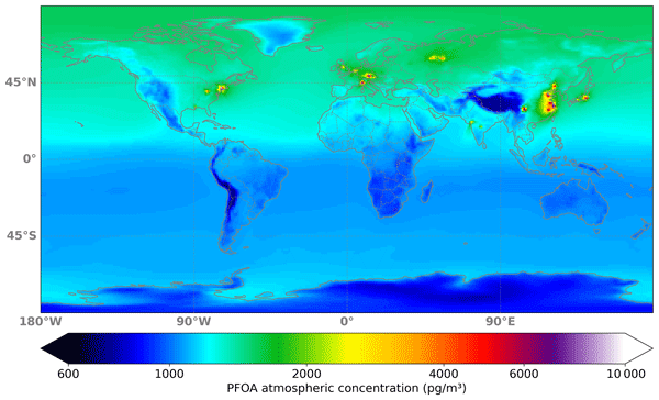
Figure 7 shows the global spatial pattern of PFOA in the period 2005–2019. The highest PFOA concentrations appear in urban and industrialized areas. East Asia shows particularly high concentrations over eastern China and Japan, a pattern likely due to the region's high industrial density and manufacturing of PFOA-containing products. Similarly, Central Europe and the UK exhibit elevated levels in densely populated areas with extensive industrial history. In North America, high concentrations cluster in the northeastern United States, following a pattern consistent with industrial emissions throughout the simulation period.

Figure 7 PFOA mean atmospheric concentration over the period 2005–2019.

Concentrations in the Southern Hemisphere are significantly lower than in the Northern Hemisphere, with only a few cities like Hyderabad and Mumbai in India showing elevated levels. This pattern aligns with the global distribution of population and industrial and urban activity, which is predominantly concentrated in the Northern Hemisphere.

4.4.2 8 : 2 FTOH

Figure 8 displays the simulated global spatial distribution of average 8 : 2 FTOH concentrations for 2005–2019.

Figure 8 8 : 2 FTOH mean atmospheric concentration over the period 2005–2019.

The spatial distribution of 8 : 2 FTOH reflects its strong connection to industrial production and population density. The highest concentrations appear in developed regions of the Northern Hemisphere, while remote areas, oceans, and the Southern Hemisphere show significantly lower levels.

Consistent with PFOA distribution, the highest 8 : 2 FTOH concentrations in North America occur primarily in the northeastern United States. In Europe, high values are concentrated in the central and western regions, reflecting the area's extensive industrial legacy and production of fluorinated consumer goods. East Asia also shows high concentrations, particularly in the industrialized and densely populated regions of China and Japan.

4.4.3 PFNA

Figure 9 shows the global distribution of average atmospheric PFNA concentrations for the years 2005 to 2019. While this distribution shows some differences from the PFOA and 8 : 2 FTOH patterns, it consistently shows high concentration regions in the northeastern United States, Europe, and East Asia.

Figure 9 PFNA mean atmospheric concentration over the period 2005–2019.

In the Northern Hemisphere, the highest concentrations are observed in industrialized regions, with a prominent peak in Central and Eastern Europe, where maximum values are observed in countries with high industrial activity and population density. This phenomenon is related to the emission of PFNA from industrial facilities, manufactured products and the use of fluorinated compounds in the region. East Asia also shows high concentrations, especially in eastern China, Japan, and South Korea, reflecting a pattern consistent with the high industrial activity in these areas and the production of fluorinated compounds used in technological and commercial applications.

The northeastern United States shows the highest concentrations in North America, likely due to both historical and ongoing industrial emissions. Across other areas of the Northern Hemisphere, concentrations gradually decrease but are still detectable due to regional and synoptic-scale atmospheric transport, which disperses PFNA from major emission sources to oceanic and remote areas such as the Arctic.

In contrast, the Southern Hemisphere has significantly lower concentrations, especially in oceanic and remote areas. This is due to both lower industrial activity and limited inter-hemispheric atmospheric transport capacity despite the persistence of PFNA.

The figure highlights how urban and industrialized regions concentrate the highest levels of this pollutant, while rural, oceanic, and polar areas remain at low, but detectable levels, except for the large mountain ranges such as the Himalayas and the Andes, as well as the Antarctic mountains, where concentrations approach zero.

4.5 Sensitivity and uncertainty tests

To evaluate the sensitivity and uncertainty associated with two of the most important oxidants (reactants) and the emission inventory, we conducted eleven additional simulations (each two years long, with the first year used as spin-up). These experiments were designed to separate the influence of oxidant fields, emissions, and internal variability. The experiments were divided into two groups as follows:

• –

  Group One (Control + oxidant sensitivity):

  • –

    Control experiment using the POPE “Best Guess” emission scenario.

  • –

    Four oxidant sensitivity experiments, where OH and RO₂ concentrations are scaled (×0 and ×10) to explore the sensitivity of PFCA formation to these reactants

• –

  Group Two (emission uncertainty and initialization):

  • –

    Six emission-uncertainty experiments using the Upper Bound (UB) and Lower Bound (LB) POPE emission scenarios, each initialized at three different times; centered on 1 January 2006 (0), one month before (M1), and one month after (P1). This to estimate internal variability associated with different initial conditions.

To systematically interpret the results of these simulations, four distinct statistical analyses were applied: (1) Relative Mean Difference (RMD) to quantify percentage changes in PFCA concentrations relative to the Control; (2) Statistical Significance Testing (ANOVA for oxidant sensitivity and Paired Permutation Tests for emission uncertainty) to assess the robustness of spatial differences; (3) Linearity Analysis to determine if PFCA production responds proportionally to changes in radical concentrations; and (4) Signal-to-Noise Ratio (SNR) analysis to distinguish the emission signal from the model's internal chaotic variability.

First, the RMDs of annual mean PFOA and PFNA concentrations were calculated for both groups relative to the Control experiment. For the second group, RMDs were also computed between simulations with different initialization days (Tables E1–E5 and Figs. E1–E4 in Appendix E).

In addition, an analysis of variance (ANOVA) was applied to the group one experiments, whereas a Paired Permutation Test (PPT) was used for the second group because the experiments in principle share a common emission origin. Together, these tests were used to assess the statistical significance of differences in spatial patterns (Tables E2–E5).

The analysis demonstrates that uncertainties in POPE emissions (UB vs. LB) lead to substantially larger variations in PFOA and PFNA concentrations compared to differences arising from varying initialization dates. This indicates that emission uncertainty is a primary driver of PFCAs dispersion within the model system (Figs. E3 and E4).

RMD analysis for the first group of simulations shows that variations on OH and RO₂ radicals have an impact on PFOA production. However, for PFNA that influence can be seen only with respect to OH, whereas sensitivity to RO₂ is negligible (Figs. E1 and E2). These findings are also supported by Table E1, which presents ANOVA test results obtaining that mean production levels differs significantly with varying OH and RO₂ concentrations. Despite, a noticeable exception is the relationship between PFNA and RO₂, which yielded a p-value of 0.97, exceeding the significance threshold of 0.05, even when RMD does not differ a lot in matters of percentage.

As expected, RMD values for PFOA Lower Bound (LB) and Upper Bound (UB) relative to the control experiment are larger between different emission scenarios, ranging from 41 % to 62 % (Table E2). The PPT supports this result, showing significant statistical differences with a p-Value substantially lower than 0.05. These changes are also evident in Figs. E3 and E4, where global RMD values range from +13 % to +150 % (UB) and −15 % to −75 % (LB) relative to the control experiment. For PFNA, these values are larger than for PFOA, with about +50 % to +105 % (UB) and −70 % to −80 % (LB). Additionally, the PPT shows that means for all experiments differ significantly for both pollutants, with p-values below $\mathrm{1.0}\times {\mathrm{10}}^{-\mathrm{4}}$ and Observed Differences (OD) between 40 and 60 mol mol⁻¹.

On the other hand, for the RMD analysis comparing experiments with different initialization times (0, M1, and P1) within the same emission scenario, PFOA RMD values range from −12.84 % to 6.40 % for both LB and UB scenarios. The OD ranges from −9.73 to 19.90 mol mol⁻¹ in UB and from −59.6 to 46.8 mol mol⁻¹ in LB. Meanwhile for PFNA, RMD ranges from −11.90 % to 6.22 % for both scenarios. The OD in this case spread from −73.31 to 75.90 mol mol⁻¹ in UB, and from −99.55 to 20.24 mol mol⁻¹ in LB. p-Values from the PPT are in all cases lower than $\mathrm{1.0}\times {\mathrm{10}}^{-\mathrm{4}}$, meaning that differences between experiments are statistically significant.

Additionally, we checked for the direct response from PFOA and PFNA production to OH and RO₂ radical concentrations in the model, we performed a linearity analysis test. This sensitivity test estimates whether production responds linearly or nonlinearly to changes in OH and RO₂ concentrations. The test considers three possible cases based on the three experiments – radical (OH or RO₂) ×0, ×10, and control, as follows: Perfect linearity occurs when the three experiments are perfectly aligned in a straight line, meaning that PFOA and PFNA production is directly proportional to the increase of OH and RO₂. Saturation takes place when the slope between the Control experiment and radical ×10 is smaller than the slope between radical ×0 and Control, meaning that production of PFCAs is limited by availability of precursor concentrations rather than by radical concentrations. Finally, Acceleration appear when the slope between Control and radical ×10 is larger than the slope between radical ×0 and Control, which means that high concentrations of radicals drive more efficient chemical pathways that produce PFCAs instead of other loss pathways.

Figure E5, shows the annual mean burden of radicals (OH and RO₂) on the x-axis and the annual mean of PFCAs (PFOA and PFNA) production on the y-axis. Panels (a) and (d) present PFNA annual mean burden against OH and RO₂ radical annual mean burden. Both panels indicate that radicals do not highly influence the PFNA production, instead, that radicals are driving other chemical pathways. In this particular case, even when linearity analysis shows Saturation, OH seems to contribute less than RO₂ to the mean annual burden of PFNA production. For PFOA, also the contribution of RO₂ shows a stronger saturation meaning that RO₂ is mostly used on other intermediate reactions than on the PFOA production. Besides, for OH, PFOA is showing a slight Acceleration pattern indicating exponential response of PFOA formation to the radical.

Another useful tool to estimate the sensitivity and internal uncertainty is the Signal to Noise Analysis. First, sensitivity to emissions is quantified obtaining the mean of all the respecting LB an UB experiments. The Control experiment represent its own mean, as there is only one Control simulation. The range of the uncertainty due to emissions (signal) is obtained by subtracting the LB mean from the UB mean. Figure E6b displays the uncertainty due to emission differences. Higher values indicate regions with the strongest emission influence, mainly located over Eastern North America, Central Europe, and Eastern China, as well as downwind regions.

Secondly, noise is obtained by calculating the standard deviation across all the experiments at all initialization times. This represents the internal variability (or internal noise) of the model; a metric of expected variability caused by the model's chaotic dynamics. Figure E6c depicts regions over the world where changes in the model's chaotic dynamics are most relevant; these areas are consistent with regions where the system is naturally more chaotic, such as the tropics, particularly over the open tropical oceans.

Finally, the Signal to Noise Ratio (SNR) is calculated by dividing the emission uncertainty (signal) by the internal variability (noise). Figure E6a presents the spatial distribution of this ratio, revealing that the signal strongly dominates the noise across the entire globe. As indicated by the map's uniform dark green color and the legend, 100 % of the surface area presents an SNR greater than 2, categorized as a “Strong Signal” where emissions dominate over initialization. This is further supported by the SNR statistics located into the box at the upper right of the map, showing a high global mean SNR of 18.66 and a median of 19.05. These values confirm that the variability driven by the different emission scenarios is significantly larger than the model's internal chaotic variability, ensuring that the detected emission impacts are robust and clearly distinguishable from background noise.

5 Discussion

Our study assessed the performance of the ICON-ART PRIEST extension in simulating atmospheric concentrations and wet deposition of PFOA, PFNA, and 8 : 2 FTOH over a time period of 15 years (2005–2019). While our evaluation shows that the model generally reproduces large-scale spatial patterns, and long-range transport, a closer look at the results reveals systematic discrepancies that carry important implications for both our understanding of atmospheric processes and future model development.

The model overestimates PFOA concentrations over Europe while underestimating them over East Asia and the Americas. In Africa, where industrial activity is low and sites are far from the main Northern Hemisphere transport pathways, the relatively small discrepancies of a few picograms per square meter suggest the model accurately represents background concentrations. However, in remote areas near major transport pathways like global circulation wind patterns and Jet Streams (particularly in Norwegian, Canadian, and Finnish locations) concentrations are overestimated by at least half an order of magnitude. This overestimation in remote Arctic areas suggests either an overemphasis of long-range transport processes or insufficient representation of removal mechanisms like scavenging. These discrepancies might stem from the model's lack of ice nucleation processes for PFCA-enriched mixed aerosols or from the assumptions about gas-to-water dissolution rates. Thackray et al. (2020) also highlights the importance of PFCA production through degradation rather than direct emissions in remote areas. Over Northern Norway (70° N), Stemmler and Lammel (2010) reported atmospheric concentrations of 4.4 to 8.9 pg m⁻³ during the year 2005, similar to the values gotten from the ICON-ART PRIEST simulations for PFOA for Andoya, Norway (69.27° N) during the year 2012 (5.75 pg m⁻³).

Our simulations show an underestimation pattern of 8 : 2 FTOH in urban and industrial regions (Fig. A2), while remote sites such as Villum Research Station exhibit close agreement between observations and modeled values. This discrepancy likely stems from either underestimated emissions of 8 : 2 FTOH in densely populated areas (where these compounds are primarily emitted) or the model's coarse spatial resolution causes a smoothing out of the existing small-scale emission gradients. While chemical degradation processes might be overrepresented, leading to lower simulated concentrations, this explanation conflicts with the absence of consistent PFOA and PFNA overestimation, which are the final products of 8 : 2 FTOH degradation. Besides that, Stemmler and Lammel (2010) found that Arctic concentrations should range from 1 to 5 pg m⁻³ (in the Canadian Arctic), aligning with our simulated values at Villum Research Station. Additionally, also Stemmler and Lammel (2010) reported daily concentrations between 0.01 and 16.4 pg m⁻³, with a monthly mean of 1.5 pg m⁻³ over the Irish West Coast. Our simulated value of 3.45 pg m⁻³ at Mace Head (Irish West Coast) during the early Spring of 2006, falls within the same range. Yarwood et al. (2007), reported an 8 : 2 FTOH range of below 10 pg m⁻³ in the Northern Atlantic to 20 pg m⁻³ in the Canadian and Norwegian Arctic, which is consistent with the values obtained by ICON-ART PRIEST in the Villum Research Station (Station Nord).

Regarding PFNA, the general tendency to overestimate could be due to regional emissions uncertainties (i.e. overestimation) or an inadequate treatment of removal processes. Contrarily, underpredictions at certain U.S. sites point at either a local underestimation of emissions or at missing chemical pathways that contribute to PFNA formation. This indicates the need to refine chemical transformation schemes and better characterize source contributions. Thackray et al. (2020) has noted that uncertainty in direct PFNA emissions contributed to deposition underestimation in their simulations. Similarly, our simulations may overestimate atmospheric PFNA concentrations due to underestimated deposition rates. This aligns with our PFNA wet deposition results (Fig. 5), which show values approximately half of those observed in certain North American regions (Albany, Slingerlands, and Sibley) and Japanese locations (Kawaguchi and Tsukuba).

An analysis of the modeled versus observed air concentrations (pg m⁻³) reveals, compound-specific biases in the model's predictive performance. For PFNA, the model shows a general tendency toward overestimation, particularly for European sampling sites; though most predictions remain within a single order of magnitude of the observations (Fig. D2 in Appendix D). Contrariwise, the model systematically underestimates PFOA concentrations across all evaluated global regions (Africa, Americas, East Asia, and Europe), with the majority of data points clustering between the 1 : 5 and 1 : 10 underestimation boundaries, indicating a consistent negative bias that may stem from missing emission sources, overly rapid simulated atmospheric deposition or unaccounted weather phenomena non captured by the model (Fig. D1). Finally, the predictive accuracy for 8 : 2 FTOH do not describe a clear pattern compared to the PFCAs; the data exhibits large variance, with multiple predictions for both the Americas and Europe falling well outside the factor-of-ten agreement band, showing significant current limitations in accurately capturing the air concentrations of this volatile precursor (Fig. D3).

Our analysis of wet deposition for PFOA and PFNA (Fig. 5) reveals that the model generally underestimates observed deposition rates by about a factor of two, particularly in urban and industrialized regions. This discrepancy carries several important implications for our understanding of atmospheric removal processes and the subsequent environmental fate of these compounds. Thackray et al. (2020) showed in their study that deposition rates vary globally across different orders of magnitude because of the precipitation patterns as the major driver of wet deposition for PFCAs removal. Consistently, our results have shown that the highest deposition rates of PFCAs are located near and downwind of densely populated regions. Yarwood et al. (2007) found that for the continental US, the range for PFOA wet deposition is between 410 to 4200 ng m⁻², our simulation results for PFOA wet deposition in Albany and Slingerlands are consistent with that range, being 980.22 and 982.8 ng m⁻², respectively. Similarly, simulated values for PFNA wet deposition on these sites were 1036 ng m⁻² for Albany and 1041 ng m⁻² for Slingerlands, fitting into the range given by Yarwood et al. (2007) for the continental US (120 to 1700 ng m⁻²).

The consistent underestimation of wet deposition across multiple sites indicates a systematic bias that may arise from the coarse resolution of meteorological inputs or an incomplete representation of aerosol-cloud interactions. Further refinement is needed, either through improved parameterizations of scavenging processes by incorporating other in-cloud processes, such as the ice nucleation of PFCAs in enriched mixed aerosols, as well as higher resolution to capture the spatial and temporal variability of precipitation more accurately (currently underestimated by a factor of two). So, this could positively affect the physical pollution removal process.

The model is able to capture very well the latitudinal trend of 8 : 2 FTOH from mid-latitudes in the Northern Hemisphere to tropical latitudes in the Southern Hemisphere. Analyzing the latitudinal gradient shows an increase in concentrations towards mid-latitudes. Even when measurements from the “Polarstern ANTXXIII-1” cruise do not cover higher latitudes than mid-latitudes, this can be an indicator that long-range transport from emissions in main industrial and urban centers in mid-latitudes is a key mechanism driving the Arctic pollution. These results are consistent with 8 : 2 FTOH concentrations measured in the Canadian Arctic and the North Atlantic Arctic (58–70° N) by Stemmler and Lammel (2010) who reported 4.16 to 22.7 pg m⁻³ during July 2006.

Oceanic regions, polar areas, and remote parts of the Southern Hemisphere show substantially lower concentrations, representing almost residual levels compared to industrialized regions. This pattern likely results from this pollutant's relatively short atmospheric lifetime.

Concerning the spatial patterns, global maps (Figs. 7–8) for PFOA, PFNA, and 8 : 2 FTOH highlight clear high pollution patterns in industrialized and densely populated regions, predominantly located in the Northern Hemisphere. Peak concentrations are observed in East Asia, Central Europe, and the northeastern United States (areas characterized by intensive industrial activity). Urban centers and industrial zones consistently show elevated levels of these compounds, while remote regions and oceans exhibit significantly lower concentrations. This strong contrast highlights the importance of local emissions in determining overall distribution patterns and demonstrates the model's capability to capture large-scale transport from emission sources to receptor regions.

The highest PFOA concentrations (Fig. 7) from the time average are found in urban areas of the northeastern United States (9000 pg m⁻³), Central Europe, and East Asia (7200 to 7800 pg m⁻³). Remote regions like the Arctic show maximum concentrations about five to six times lower (1400 to 1600 pg m⁻³). Since emission sources are primarily in the Northern Hemisphere, the Southern Hemisphere has even lower maximum concentrations than the Arctic (∼1100 pg m⁻³).

PFNA follows a similar pattern (Fig. 9), with maximum concentrations of approximately 4700 pg m⁻³ in the eastern United States, and slightly lower levels over Europe and East Asia (3700 to 3900 pg m⁻³). Arctic concentrations are lower (2400 pg m⁻³) but exceed PFOA levels, with the Southern Hemisphere showing a similar behavior (2200 pg m⁻³).

8 : 2-FTOH (Fig. 8) shows significantly lower concentrations than both PFCAs, measuring around 50 pg m⁻³ in the northeastern United States and Central Europe, and approximately 20 pg m⁻³ in East Asia. Remote regions, including the Arctic and Southern Hemisphere, show concentrations of about 5 pg m⁻³.

The patterns differ in both distribution and magnitude due to several factors. These include the compounds half-life (5–10 d for 8 : 2 FTOH, 90–349 d for PFOA and PFNA) (Stemmler and Lammel, 2010; Wallington et al., 2006; Environment Canada, 2010), the deposition and chemical degradation of 8 : 2 FTOH, and the production of PFOA and PFNA from precursors through reaction mechanisms. The distribution and rates of emissions also play a key role. For PFOA, more detailed considerations are made, while PFNA and 8 : 2 FTOH emissions are scaled based on population density and GDP in regions outside the United States and Europe (See Sect. 3.1.2).

Global patterns in our simulation are similar to Stemmler and Lammel (2010), showing the distribution of 8 : 2 FTOH primarily over mid-latitudes. PFOA global distribution is more widely spread, especially from mid-latitudes towards the Arctic; even so, concentrations southward decrease less abruptly than the 8 : 2 FTOH gradient.

Overall, while the model robustly captures the general trends in latitudinal and global distributions, the identified discrepancies point to a need for further refinement in emission inventories, scavenging, chemistry and transport mechanisms.

6 Conclusions

The ICON-ART PRIEST model extension represents a significant advancement in simulating the atmospheric fate of PFCA precursors and their transformation products. Integrating an enhanced chemical mechanism that couples both gas-phase and aqueous-phase processes with a detailed, temporally resolved PFAS emission inventory, ICON-ART PRIEST offers the possibility of representing PFCA formation processes, their long-term global transport, and their removal mechanisms.

Our evaluation demonstrates that ICON-ART PRIEST successfully reproduces the broad-scale spatial patterns and latitudinal gradients observed in the atmosphere, underscoring the critical role of long-range transport from industrial and urban centers in driving Arctic pollution and the importance of precursors.

The overestimation of atmospheric concentrations in remote areas indicates a need for improved modeling of transport and deposition processes. Such as incorporating in-cloud processes as ice nucleation and cloud condensation with mixed aerosols enriched with PFCAs. In contrast, underestimations in major urban centers indicate that the local emissions assumed by POPE may be too low, or that missing source categories and secondary formation processes are more significant than currently accounted for. Additional features, such as kinetics considering Secondary Inorganic Aerosol (SIA) formation, could also be beneficial to address both overestimation in low-emission areas and underestimation in densely populated or heavily industrialized locales. Sulfate and nitrate rich liquid film that forms on SIA particles works as an acidic reactor; its high water content and low pH accelerate the aqueous-phase oxidation and hydrolysis of volatile PFAS precursors (such as fluorotelomer alcohols, e.g. 8 : 2 FTOH), rapidly converting them into PFCAs. Also, the same wet, acidic medium strongly favors partitioning into the particle phase. Furthermore, our study pushes forward in the necessity to improve the measurement campaigns' efforts, looking for an increase in the amount of data and improving the quality by using, for example, High Volume Samplers instead of passive methods with limited detection problems. This would also allow us to perform validations and discover potential new patterns on the PFCAs fate.

While the current ≈ 105 km² grid resolution is an improvement compared to previous global studies, higher spatial resolution is still needed. Local features and processes significantly affect PFCA concentrations in industrial and populated areas. A finer grid resolution would better capture local sources and weather patterns, in particular precipitation events.

This work highlights the value of coupled atmospheric chemistry and transport modeling in addressing environmental and regulatory challenges associated with PFCAs by providing new tools to represent concentrations and spatial distribution of these pollutants. ICON-ART PRIEST offers a robust and versatile platform for examining the fate and transport of PFOA and PFNA on regional and global scales. Such work will ultimately support more effective environmental management, inform regulatory decisions, and help protect ecosystems and human health from the persistent challenges introduced by PFCAs and FTOHs like 8 : 2 FTOH.

Appendix A

A1 Chemical compounds, and Sampling sites locations

Table A1 PFAS included in the POPE emission inventory. The compounds used for this study are marked with an asterisk.

Table A2 Observation sites and period of sampling per compound, PFOA, 8 : 2 FTOH and PFNA.

Appendix B: Reaction Mechanism

Table B1 Gas-phase reactions (Thackray et al., 2020), TEMP is the temperature in K.

^a Young and Mabury (2010), ^b Burkholder et al. (2015), ^c Wallington et al. (2006), ^d Yarwood et al. (2007).

Table B2 Photolytic reactions (Thackray et al., 2020). “jx” is the indicator for JVAL photolysis module, “ip_SPECIE” is the prefix calling the reaction rate into the MECCA equation file.

^* Young and Mabury (2010).

Table B3 Aqueous-phase reactions, Reaction rate (K1, K2, “TEMP” is the temperature in K, and “LWC” is the liquid water content volume ratio m³ m⁻³). Based on Sander (2023).

^a Arp et al. (2006), ^b Kutsuna and Hori (2008), ^c Abusallout et al. (2022), ^d Endo et al. (2023).

Appendix C: Glossary

List of acronyms and abbreviations.

Acronym	Definition
AFFF	Aqueous Film Forming Foam
ART	Aerosol and Reactive Tracers
CAM-chem	Community Atmospheric Model with Chemistry
CESM	Community Earth System Model
CLM	Climate Limited-area Modelling (Community)
DWH	Data Warehouse (GMP data repository)
EBAS	EMEP Database for Atmospheric Composition
ECMWF	European Centre for Medium-Range Weather Forecasts
EMEP	European Monitoring and Evaluation Programme
ERA-Interim	Global atmospheric reanalysis dataset (ECMWF)
GMP	Global Monitoring Plan (Stockholm Convention)
HPC	High Performance Computing/Cluster
ICON	ICOsahedral Non-hydrostatic model
ICON-ART	ICON with Aerosol and Reactive Tracers
ICON-ART PRIEST	ICON-ART with PFAS Reactions In Earth System Transport
KPP	Kinetic Pre-Processor
LB/UB	Lower Bound/Upper Bound (in scenarios)
LWC	Liquid Water Content
MECCA	Module Efficiently Calculating the Chemistry of the Atmosphere
MOZART-T1	Model of OZone and Related chemical Tracers (CAM-chem mechanism)
NMB	Normalized Mean Bias
NO/NO2	Nitrogen oxides
OH/HO2/RO2	Hydroxyl, hydroperoxyl, and organic peroxyl radicals
PFAS	Per- and Polyfluoroalkyl Substances
PFCAs	Perfluoroalkyl Carboxylic Acids
PFECAs	Perfluoroether Carboxylic Acids
PFSAs	Perfluorosulfonic Acids
POPE	Persistent Organic Pollutant Emissions model
PRIEST	PFAS Reactions In Earth System Transport
RMSE	Root Mean Square Error
SLEVE	Smooth Level Vertical coordinate
SPICE	Starter Package for ICON-CLM Experiments
UNEP	United Nations Environment Programme

Table C1 PFAS and chemical-related substances definitions.

Appendix D: Observed vs. modeled factor plots

Figure D1 Comparison of observed versus modeled PFOA concentrations (pg m⁻³) by region on a log-log scale. The solid line represents 1 : 1 agreement, with dotted lines indicating deviations by factors of 2, 5, and 10.

Figure D2 Comparison of observed versus modeled PFNA concentrations (pg m⁻³) by region on a log-log scale. The solid line represents 1 : 1 agreement, with dotted lines indicating deviations by factors of 2, 5, and 10.

Figure D3 Comparison of observed versus modeled 8 : 2 FTOH concentrations (pg m⁻³) by region on a log-log scale. The solid line represents 1 , 1 agreement, with dotted lines indicating deviations by factors of 2, 5, and 10.

Appendix E: Sensitivity tests

Table E1 Relative mean differences and ANOVA test for OH and RO₂ sensitivity experiments.

Figure E1 Relative Mean Differences (%) in annual mean atmospheric concentrations of PFOA (top) and PFNA (bottom). Panels show sensitivity experiments for OH ×0 (left) and OH ×10 (right) relative to the control simulation.

Figure E2 Relative Mean Differences (%) in annual mean atmospheric concentrations of PFOA (top) and PFNA (bottom). Panels show sensitivity experiments for RO₂ ×0 (left) and RO₂ ×10 (right) relative to the control simulation.

Table E2 PFOA Relative mean differences and Paired Permutation Test for LB and UB against Control sensitivity experiments.

Table E3 PFNA Relative mean differences and Paired Permutation Test for LB and UB against Control sensitivity experiments.

Table E4 PFOA relative mean differences and Paired Permutation Test for LB and UB in their different corresponding initialization period.

Table E5 PFNA relative mean differences and Paired Permutation Test for LB and UB in their different corresponding initialization period.

Figure E3 Relative mean differences PFOA from different initialization times. (a) LB 0 vs. Control, (b) LB M1 vs. Control, (c) LB P1 vs. Control, (d) UB 0 vs. Control, (e) UB M1 vs. Control, (f) UB P1 vs. Control.

Figure E4 Relative mean differences PFNA from different initialization times. (a) LB 0 vs. Control, (b) LB M1 vs. Control, (c) LB P1 vs. Control, (d) UB 0 vs. Control, (e) UB M1 vs. Control, (f) UB P1 vs. Control.

Figure E5 Linearity analysis of global annual mean burdens of PFNA and PFOA. Panels (a)–(b) show the response to RO₂ and (c)–(d) to OH. The model response (solid line) is compared against a linear fit (dashed red line) across three points: radical removal (×0), base case (control), and a ten-fold increase (×10). The deviation of the solid line from the dashed line represents the non-linear chemical feedback of the system.

Figure E6 Signal to noise ratio analysis, emissions vs. initialization time (a) Signal to Noise Ratio (SNR): Emission sensitivity vs. initialization uncertainty. (b) Signal: Emission sensitivity, absolute value from differences of all UB initializations and LB initializations. (c) Noise: Internal variability, standard deviation from all the initializations.