Accurate and robust geometric algorithms for regridding on the sphere

Regridding is one of the most common operations in geoscientific modeling and data analysis. There are many types of regridding, each drawing from a common set of fundamental computational geometry algorithms. However, these algorithms are rarely documented together or systematically compared in a manner that elucidates their relative strengths and appropriate use. In particular, several recent studies have highlighted the importance of careful treatment of floating point operations in the implementation of these algorithms to ensure numerical robustness and stability. In this work, we organize non-conservative and conservative regridding operations end-to-end, from spatial indexing, great-circle and constant latitude geometry, and spherical predicates to spherical clipping, triangulation, and area calculation with constant latitude corrections, into a coherent set of geometric kernels on the sphere. When known, we present numerically stable floating-point formulas and characterize their error behavior. We also indicate where higher-precision techniques, such as Error-Free Transformations, can be incorporated when additional accuracy is needed. The resulting framework establishes a practical and performance-portable baseline for accurate and robust regridding on the sphere.

1 Introduction

The regridding operation is essential to geoscientific modeling and data analysis. Accurate, property-preserving regridding is essential to ensure that model couplers, data assimilation systems, and diagnostic analyses preserve physical consistency across grids (Ullrich and Taylor, 2015; Ullrich et al., 2016; Marsico and Ullrich, 2023). However, despite the importance of this operation, the geometric algorithms that underpin regridding on the sphere are poorly documented and are implemented with varying degrees of rigor, robustness, and accuracy across community tools.

This paper provides a systematic examination of the geometric and numerical foundations of spherical regridding. We establish a unified framework for representing grids on the sphere – defining points, edges, and polygonal faces in a way that aligns geoscientific conventions with computational geometry formalisms. Within this framework, we describe, analyze, and compare the key algorithms required for regridding. We use ^* to denote operations for which suitable algorithms exist in the geoscience software packages but are, to our knowledge, systematically documented here for the first time, and ${}^{**}$ to denote operations for which no suitable algorithms currently exist and for which we propose new methods. The algorithms examined in this work include:

• face centerpoint computation and spatial indexing,

• interior maximum-latitude evaluation along great-circle arcs^*,

• numerically stable edge-length computation,

• segment-segment intersection algorithms for both great-circle–great-circle and great-circle–constant-latitude pairs${}^{**}$,

• spherical point-in-face predicates${}^{**}$,

• bounding-volume filtering^*,

• candidate-face identification for mesh overlay (advancing-front arrangement versus local face search)^*,

• spherical clipping and triangulation, including area computation and constant-latitude edge correction^*,

• construction of conservative regridding maps^*.

Each operation is examined in terms of its mathematical formulation, numerical stability, and efficiency.

The Computational Geometry Algorithms Library (CGAL) (The CGAL Project, 2024) is widely regarded as the reference implementation for robust geometric computation, underpinning much of the theoretical development in computational geometry. Although CGAL is not used in geoscience software and does not appear in our benchmarks, it provides the most complete suite of exact geometric algorithms available today. In this paper, we reference CGAL's formulations as the canonical baseline for each geometric operation. However, CGAL's reliance on exact arithmetic limits vectorization of its kernels. Although CGAL algorithms can be parallelized, the resulting implementations incur high computational overhead, motivating comparison with floating-point formulations used in geoscientific software packages TempestRemap (Ullrich and Taylor, 2015; Ullrich et al., 2016), UXarray (UXarray Organization, 2024), and YAC (Hanke et al., 2016). Throughout this paper, references to these packages correspond to TempestRemap v2.2.0, UXarray v2025.08.0, YAC v3.9.0, and CGAL v6.0.1, which were the latest available versions at the time of writing.

Where existing methods are incomplete, numerically unstable, or unavailable, we propose new algorithms to fill these gaps. Specifically, we introduce (i) an accurate and efficient great-circle arc intersection algorithm based on Chen et al. (2026) (Sect. 5.3); (ii) a geometrically consistent construction of spherical bounding boxes (Sect. 5.7) together with a robust point-in-polygon test and a triangulation procedure tailored to unstructured geoscientific grids (Sect. 5.6); (iii) an area-correction method for triangles with constant-latitude edges and a formulation for computing centroids of arbitrary spherical faces without triangulation (Sect. 5.10.1 and 5.5); and (iv) a suite of spherical overlay algorithms optimized for regridding and integration workflows (Sect. 4). Selected components, including the intersection algorithms, latitude-longitude bounds, and point-in-polygon predicates, are implemented in an SIMD-efficient C$++$ library, AccuSphGeom (Chen, 2026), to support easy adoption in other codebased.

While this paper intends to document the present state-of-the-art in computational geometry for the sphere, novel efforts to further improve accuracy and robustness have recently emerged and may lead to better algorithms in the near future. For instance, Error-Free Transformations (EFTs) rely on the fact that round-off errors in primitive floating-point operations – addition or multiplication – are themselves floating-point numbers that can be computed with simple algorithms (Knuth, 1997; Graillat, 2009; Ogita et al., 2005). EFTs for spherical geometry calculations, such as those developed in Chen et al. (2026) have the potential to compensate for floating-point errors and increase algorithm accuracy. Additionally, with vectorization and parallelization, EFT-based algorithms can achieve essentially the same runtime cost as standard floating-point implementations.

By combining theoretical rigor with implementation-level analysis, this study bridges the gap between computational geometry and geoscientific modeling practice. The resulting set of recommended algorithms provides a reproducible, performance-portable foundation for next-generation regridding and integration tools on the sphere.

2 Terminology and problem definition

We begin by specifying the terminology and notational conventions used throughout this paper. For simplicity, we assume that the domain of our operations is the unit sphere.

2.1 Nodes

A node refers to a particular location on the unit sphere and is stored either using longitude-latitude (λ,ϕ) coordinates or 3D Cartesian coordinates $(x,y,z)$, subject to $x^{\mathrm{2}}+y^{\mathrm{2}}+z^{\mathrm{2}}=\mathrm{1}$. Conversion between these two coordinate systems is given by:

$$\begin{array}{}\text{(1)}& \begin{array}{rl}& x=\cos \mathit{\lambda }\cos \mathit{\varphi },\mathit{\lambda }=\mathrm{atan}\mathrm{2}(y,x),\\ & y=\sin \mathit{\lambda }\cos \mathit{\varphi },\mathit{\varphi }=\mathrm{asin}\left(z\right),\\ & z=\sin \mathit{\varphi }.\end{array}\end{array}$$

2.2 Edges

An edge is defined as a line or curve lying on the unit sphere that connects two nodes (referred to as the endpoints of the edge). The focus of this work is on the two most commonly employed edge types in geoscience as of the time of writing: great circle arcs (GCAs) and lines of constant latitude (LCLs). Note that lines of constant longitude are also GCAs (Taylor, 2024).

In both cases, edge parameterizations are constructed from a common auxiliary linear interpolation between endpoints. Given endpoints ${\mathit{x}}_{\mathrm{1}}=(x_{\mathrm{1}},y_{\mathrm{1}},z_{\mathrm{1}})$ and ${\mathit{x}}_{\mathrm{2}}=(x_{\mathrm{2}},y_{\mathrm{2}},z_{\mathrm{2}})$, we define

$$\begin{array}{}\text{(2)}& \stackrel{\mathrm{̃}}{\mathit{x}}=(\mathrm{1}-a){\mathit{x}}_{\mathrm{1}}+a{\mathit{x}}_{\mathrm{2}},a\in [\mathrm{0},\mathrm{1}].\end{array}$$

For GCAs, the edge is defined as the intersection between the unit sphere and the unique plane passing through the two endpoints and the origin. The parameterized curve is obtained by normalizing the auxiliary interpolation:

$$\begin{array}{}\text{(3)}& \mathit{x}=\stackrel{\mathrm{̃}}{\mathit{x}}/\parallel \stackrel{\mathrm{̃}}{\mathit{x}}\parallel .\end{array}$$

This parameterization can only be used when the arc subtends less than 180°. If a GCA subtends exactly 180°, then the endpoints are insufficient to define the GCA uniquely.

LCLs are defined by the intersection of the unit sphere with a plane of constant z=z₀ and require that both endpoints satisfy $z_{\mathrm{1}}=z_{\mathrm{2}}=z_{\mathrm{0}}$. Writing $\stackrel{\mathrm{̃}}{\mathit{x}}=(\stackrel{\mathrm{̃}}{x},\stackrel{\mathrm{̃}}{y},\stackrel{\mathrm{̃}}{z})$, the LCL parameterization is given by:

$$\begin{array}{}\text{(4)}& \begin{array}{rl}\mathit{x}& =\left(\sqrt{\mathrm{1}-z_{\mathrm{0}}^{\mathrm{2}}}{\displaystyle \frac{\stackrel{\mathrm{̃}}{x}}{\sqrt{{\stackrel{\mathrm{̃}}{x}}^{\mathrm{2}}+{\stackrel{\mathrm{̃}}{y}}^{\mathrm{2}}}}},\sqrt{\mathrm{1}-z_{\mathrm{0}}^{\mathrm{2}}}{\displaystyle \frac{\stackrel{\mathrm{̃}}{y}}{\sqrt{{\stackrel{\mathrm{̃}}{x}}^{\mathrm{2}}+{\stackrel{\mathrm{̃}}{y}}^{\mathrm{2}}}}},z_{\mathrm{0}}\right),\\ & a\in [\mathrm{0},\mathrm{1}].\end{array}\end{array}$$

This parameterization similarly requires that the endpoints of the edge are within 180° of longitude.

Although we focus exclusively on GCAs and LCLs, we acknowledge the conspicuous need for algorithms and software that correctly handle the many other types of spherical grid arcs now being used in geoscientific models. For instance, there has been recent interest in alternative spherical grids such as HEALPix or tripolar grids. HEALPix was originally developed for mapping cosmological background radiation, but is now being considered as a common quasi-uniform grid for sharing and intercomparing Earth system data (Gorski et al., 2004). The HEALPix grid is a hierarchical equal-area subdivision of the sphere that trivializes coarsening and refinement operations. Tripolar grids (Madec and Imbard, 1996) are also widely used in ocean models such as NEMO (Madec and the NEMO System Team, 2024) and employ a hybrid construction consisting of regular Mercator parallels and meridians in low latitudes, and curved confocal ellipses with their orthogonal normals in polar regions, all mapped onto the sphere. At present, most spherical geometry codes approximate these less common cell boundaries using GCAs or LCLs, and their correct geometric handling remains an area of open research. Despite it being common to use different edge types interchangeably (e.g., approximating LCLs as GCAs), doing so changes the underlying integration domain. While approximation errors can shrink with increasing resolution for smooth line integrals, regridding depends on discrete geometric predicates such as intersection detection, cyclic ordering, and point-in-face tests that determine the topology of the supermesh. Small geometric perturbations can therefore flip these predicates, leading to misclassified or collapsed edges and invalid overlap polygons. Moreover, conservative remapping requires accurate overlap areas, and geometric approximation errors can accumulate across many cells and need not vanish, particularly for nonsmooth fields. Geoscientific analysis packages tend to use approximate algorithms because of their relative simplicity, and because robust, geometrically correct algorithms are hard to find or implement – an issue we aim to overcome with this work.

2.3 Faces

A face (sometimes referred to as a polygon or cell in the literature) is defined as an ordered set of non-intersecting edges. By convention, we assume edges are listed counterclockwise, as oriented inward from outside the sphere. Nodes that are part of a face may also be referred to as its vertices. We further assume that each face is entirely contained within a single arbitrarily oriented hemisphere so that the face does not contain the antipode of any of its interior points.

2.4 Meshes and supermeshes

A mesh is a set of non-overlapping faces that cover, or partially cover, the unit sphere and provide the geometric partition and neighborhood relations needed to represent and process spatial fields. Meshes are also sometimes referred to as grids, although the term “grid” normally suggests some regularity in the location of nodes and can refer to an array of grid points without explicit faces or edges.

A supermesh refers to the common, auxiliary mesh generated by overlaying two meshes, with new intersection nodes, edges, and faces being defined as necessary to ensure the faces of the supermesh are non-overlapping (e.g., Farrell et al., 2009).

In geoscientific models using finite-volume methods, data is commonly stored as face averages. However, in some models, data values are staggered so that they are instead associated with vertices, edges, or other special nodal locations (e.g., when using finite-element methods; see Sect. 5). Often staggering of data can also be interpreted as using multiple offset meshes within a single model (e.g., vertex duals or edge duals) (Arakawa and Lamb, 1977). Each independent data value associated with a mesh entity is referred to as a degree of freedom of the mesh. In many geoscientific applications, the quantity of interest is the integral of the stored field over the mesh. In this case, the integral can be computed as a dot product of a vector of data values and a vector of associated weights. For face-averaged data, the weights are simply the face areas.

2.5 Maps and linear maps

A map is an operator that transforms data on a source mesh, with N_s degrees of freedom, to a target mesh, with N_t degrees of freedom. In this paper we are primarily interested in linear maps, typically represented as a sparse matrix operator $\mathsf{R}\in {\mathbb{R}}^{N_{\mathrm{t}}\times N_{\mathrm{s}}}$ that can operate on the vectorized source mesh data ${\mathit{\psi }}^{\mathrm{s}}\in {\mathbb{R}}^{N_{\mathrm{s}}}$ to produce the vectorized target mesh output ${\mathit{\psi }}^{\mathrm{t}}\in {\mathbb{R}}^{N_{\mathrm{t}}}$, i.e.,

$$\begin{array}{}\text{(5)}& {\mathit{\psi }}^{\mathrm{t}}=\mathsf{R}{\mathit{\psi }}^{\mathrm{s}}.\end{array}$$

Ullrich and Taylor (2015) discuss desirable properties of 𝖱 that are relevant to regridding. Consistency requires that constant fields be mapped to constant fields, equivalent to the row-sums of 𝖱 being equal to 1. Monotonicity requires that no new extrema be created by application of 𝖱, equivalent to 𝖱 being consistent coefficients in the range [0,1]. For a map to be conservative, the global quadrature rule for the source and target meshes must evaluate to the same value, i.e.,

$$\begin{array}{}\text{(6)}& \sum _i{J}_i^t{\mathit{\psi }}_i^t=\sum _j{J}_j^{\mathrm{s}}{\mathit{\psi }}_j^{\mathrm{s}},\end{array}$$

where $J_j^{\mathrm{s}}$ and $J_i^{\mathrm{t}}$ refer to the weights of each degree of freedom on the source and target meshes, respectively.

In general, a conservative linear map will take the form

$$\begin{array}{}\text{(7)}& {\mathsf{R}}_{ij}={\displaystyle \frac{J_{ij}^{\mathrm{ov}}}{J_i^{\mathrm{t}}}},\end{array}$$

with

$$\begin{array}{}\text{(8)}& \sum _i{J}_{ij}^{\mathrm{ov}}=J_j^{\mathrm{s}}.\end{array}$$

Namely, $J_{ij}^{\mathrm{ov}}$ distributes the source degree of freedom among target degrees of freedom so that mass is conserved under global quadrature. If degrees of freedom represent face averages, then the $J_{ij}^{\mathrm{ov}}$ is most logically given by the area of the intersection of source mesh face j and target mesh face i. Thus the two-step process of generating a supermesh and computing its face areas is one means of generating conservative map coefficients.

3 Overview of regridding

Regridding is the process of transferring fields between meshes of differing resolutions and topologies using a mapping operator. Nodal regridding methods, such as nearest-neighbor or inverse-distance, operate on data stored at nodal points or at face centroids. Volumetric regridding methods, which are the focus of this paper, instead operate on face-averaged values. In addition to the properties discussed in Sect. 2.5, locality is also desirable, and refers to regridded mass not moving far from its origin (resulting in spurious unphysical diffusion). For methods that make use of an explicit source and target mesh, locality can be achieved by requiring that regridding weights are non-zero only if two faces overlap. Nodal methods can also achieve locality by ensuring that regridding weights are zero beyond a certain distance, usually a function of the local nodes. In practice, small residual imbalances in global conservation can arise from numerical effects such as approximate area calculations, floating-point roundoff errors accumulated when summing over many cells, or discretization errors. To eliminate these discrepancies, many schemes include a post-processing adjustment that restores exact global conservation, often through a uniform normalization step (Taylor, 2024), despite such approaches typically introducing non-locality.

3.1 Non-conservative regridding

Non-conservative schemes, sometimes referred to as value-interpolating methods, do not enforce integral preservation and are appropriate when the target diagnostic does not require strict conservation of mass or energy. Examples include nearest-neighbor (a.k.a. 1-nearest-neighbor), bilinear or other polynomial-based interpolations, and inverse-distance weighting. Nearest-neighbor is local, monotone, and preserves extrema, making it especially useful for categorical variables, masks, or quick-look visualization. However, nearest-neighbor produces sharp discontinuities when adjacent samples switch between source points and so is only first-order accurate. Bilinear interpolation, which is explored in detail in Marsico and Ullrich (2023), is local, monotone, second-order accurate, and works well for smoothly varying scalar fields when conservation is not essential. Inverse-distance weighting is a robust choice on highly irregular or sparse point sets, such as station data, where constructing dual meshes or elementwise reconstructions is impractical; with a suitable weighting exponent, its accuracy can approach that of bilinear interpolation while preserving monotonicity. If a distance cutoff is imposed, inverse-distance weighting can also provide locality. Higher-order polynomial stencils are sometimes employed for smoothly varying diagnostics, though they require care near sharp gradients to avoid spurious oscillations.

Higher-order interpolation methods, such as bicubic schemes, employ larger stencils and can incorporate gradient or slope information, resulting in smoother interpolations. For instance, bicubic Hermite interpolation leverages both function values and derivatives at neighboring points. Similarly, the YAC coupler implements a hybrid cubic scheme that employs Bernstein-Bézier patches to achieve smooth cubic interpolation over arbitrary grid structures. While these higher-order methods typically reduce interpolation errors for smoothly varying fields, they may introduce unintended extrema unless specifically constrained. There also exist sophisticated interpolation methods using patch-based schemes (Khoei and Gharehbaghi, 2007; Gu et al., 2004), which are described in depth by Valcke et al. (2022, 2021).

A more recent line of work explores generalized barycentric interpolation, which extends classical barycentric coordinates to arbitrary polygonal cells (Marsico and Ullrich, 2023). This formulation incorporates multiple neighboring vertices; for example, Marsico and Ullrich (2023) showed that on icosahedral grids, using up to six neighboring vertices yields markedly smaller maximum errors than traditional bilinear or Delaunay-based interpolation. Such coordinate-based methods guarantee positive weights and adapt naturally to unstructured meshes. In parallel, the graphics community has developed extensive theory for generalizing barycentric coordinates to spherical polygons. Langer et al. (2006) introduced a general framework for defining barycentric coordinates to arbitrary convex or non-convex spherical polygons, showing how planar barycentric formulas (e.g., Wachspress (Wachspress, 1976) or mean value coordinates) can be adapted to the sphere. More recently, Aitelhad (2022) proposed an alternative construction derived directly from 3D barycentric coordinates in the ambient space. Building on these approaches, Bensad and Ikemakhen (2023) developed an explicit construction that enables spherical barycentric coordinates to be computed directly from their 2D Euclidean counterparts.

3.2 Conservative regridding

As discussed in Sect. 2.5, conservative regridding requires the calculation of the overlap weights $J_{ij}^{\mathrm{ov}}$, which can be directly obtained from the supermesh. However, since the exact mesh geometry necessary for supermesh construction can be challenging, it has been common in the geosciences to use geometric approximations, such as replacing edges by piecewise line segments and eliminating the need for a geometrically exact supermesh. Further, while some methods compute the complete supermesh explicitly, others only keep as much of the supermesh in memory as is needed for the generation of local weights. In this section we briefly review the design decisions underlying the most widely used conservative regridding packages.

From a computational geometry standpoint, supermesh construction on curved surfaces such as the sphere remains an active area of research. The Computational Geometry Algorithms Library (CGAL) (The CGAL Project, 2024) integrates robust capabilities for computing arrangements of great circle arcs and other parametric surfaces using exact computations (Wein et al., 2024; Berberich et al., 2010). In the terminology of Sect. 4.2.1, its spherical-arrangement module realizes a global advancing-front construction that builds a complete overlay of all source and target edges (Wein et al., 2024; de Castro et al., 2024). As discussed in Sect. 5.9, constructing this full overlay a priori, together with the reliance on exact computations, makes the approach impractical for extremely high-resolution meshes, for example the global simulations at resolutions ≲ 5 km introduced in Stevens et al. (2019), and difficult to parallelize efficiently at scale. Its current implementation is also limited to GCAs. Consequently, while unsuitable as a production tool for parallel regridding, CGAL is best regarded as a gold-standard baseline for geometric correctness, against which faster floating-point implementations can be validated.

The Spherical Coordinate Remapping and Interpolation Package (SCRIP) (Jones, 1999) is one of the earliest tools for generating conservative regridding weights over arbitrary meshes. It identifies overlapping faces using a hierarchical binning search that restricts candidate cells via latitude and bounding-box filtering. It computes weights using line integrals around cell boundaries in regular latitude-longitude space, treating edges as straight lines rather than GCAs. While this geometric approximation reduces fidelity, particularly in high-latitude regions (Valcke et al., 2022, 2021), the overall method is computationally efficient for large grids and supports monotonicity through an optional post-processing step.

Inspired by SCRIP, the Earth System Modeling Framework (ESMF) (ESMF Development Team, 2002–2025) offers more advanced and scalable regridding capabilities. It introduces a faster spatial indexing algorithm based on tree structures and also supports distributed-memory parallelism for efficient weight computation. It provides flexibility through support for diverse grid geometries and regridding choices. ESMF allows users to choose between two different LineTypes: with the default CART option, edges are treated as straight segments in three-dimensional space and faces as planar facets, while selecting GREAT_CIRCLE treats each edge as GCAs.

The Cascade Remapping between Spherical Grids (CaRS) (Lauritzen and Nair, 2008) package provides a high-order regridding algorithm for transferring data between regular latitude-longitude (RLL) and cubed-sphere grids, ensuring both mass conservation and monotonicity. It achieves this by approximating the two-dimensional area integral as a sequence of one-dimensional integrals along coordinate directions, which simplifies overlap geometry and enables the use of one-dimensional high-order reconstructions and limiters. While this dimensional splitting introduces a small geometric approximation error, it can be partially mitigated in practice through higher-order subcell reconstructions.

Extending SCRIP's line integral approach to certain GCAs, the Geometrically Exact Conservative Remapping (GECoRe) (Ullrich et al., 2009) performs exact geometric intersection between source and target faces and carries out 2D integration over the true overlapping region. It uses closed-form formulae tailored to specific grid types like lat-lon and cubed-sphere. Like SCRIP, it exploits grid symmetry and applies Gauss's theorem to convert area integrals into line integrals. This leads to fast and exact regridding but lacks generality: closed-form expressions must be derived for new grid types and may not be available for arbitrary grid types.

TempestRemap (Ullrich and Taylor, 2015; Ullrich et al., 2016), which is used in Energy Exascale Earth System Model (E3SM) (E3SM Project, 2024) workflows, represented a shift toward mathematically rigorous regridding. As mentioned earlier, the mathematical requirements for conservation, monotonicity, and consistency for linear maps are explicitly codified in this paper. It uses spherical geometry explicitly, treats all mesh edges as great circles, and implements a “search-and-clip” paradigm: a k–d tree identifies potentially intersecting faces, and great-circle intersections are computed exactly using spherical geometry. It supports high-order conservative and monotone regridding. To address scalability, MOAB (Mahadevan et al., 2020) integrates TempestRemap's weight computation into a parallel advancing-front search routine through an offline remapping tool, mbtempest, enabling distributed parallel execution. Similarly, XML-IO-Server (XIOS) (XIOS Development Team, 2025) follows the same great-circle representation but, to accommodate constant-latitude boundaries, approximates each parallel by many short great-circle segments, allowing the edges to more closely follow lines of latitude and thereby improve global conservation, as noted by Taylor (2024). During the development of E3SM v1, the transition from ESMF to TempestRemap was driven by the need to support spectral-element grids used in the atmospheric core, which are natively supported by the latter package. TempestRemap provides options for both conservative nodal and volumetric meshes – namely, the mesh obtained by defining volumes around each finite element node. To the best of our knowledge, this is the only package with rigorous support for both finite volume and finite element discretizations (E3SM Development Team, 2025; Mahadevan et al., 2020; Valcke et al., 2021).

A major restriction of the aforementioned regridding tools is that they only support either GCAs or LCLs as grid lines. A recently developed tool that supports both edge types is the Yet Another Coupler (YAC) (Hanke et al., 2016). YAC's geometric algorithms underpin the conservative regridding functionality of the Climate Data Operator (CDO) package (Schulzweida, 2023), and their correct treatment of geometry makes both YAC and CDO unique among geoscience libraries. Their “search-and-clip” approach uses bounding spherical caps and a modified Sutherland-Hodgman algorithm (Sutherland and Hodgman, 1974), and their regridding routines triangulate clipped faces to calculate areas. Efforts are currently underway to integrate regridding capabilities from YAC and TempestRemap into the python-based UXarray package (UXarray Organization, 2024).

In summary, despite decades of progress, geometric operations for conservative regridding on the sphere are still an area of open research. While the first regridding packages relied extensively on approximations, modern regridding codes generally aim to closely capture exact mesh geometry.

3.3 Extensions to high-order

First-order conservative methods assume a piecewise-constant reconstruction over each source face and obtain weights from the fractional overlaps of faces on the source and target. This method ensures robustness but tends to be more inaccurate for smoothly varying fields. Second-order conservative schemes reconstruct a facewise gradient vector and integrate it over each overlap polygon, thereby improving accuracy while retaining conservation. When exact face geometry is available, these methods reduce to the geometry-aware scheme of Kritsikis et al. (2017), which has been widely adopted in regridding libraries. Extending further, arbitrary-order conservative methods integrate high-order reconstructions, such as spectral-element bases, against high-order quadrature rules over the exact overlap polygons, thereby achieving conservation, consistency, and high accuracy, provided that the reconstruction matches the source discretization (Ullrich and Taylor, 2015; Ullrich et al., 2016; Valcke et al., 2022, 2021; Taylor, 2024). These conservative finite-volume and finite-/spectral-element schemes are surveyed in detail in Valcke et al. (2022, 2021). Higher-order schemes, while improving accuracy, can generate overshoots near discontinuities or steep gradients. Unfortunately, any conservative, linear regridding method (e.g., one where regridding reduces to a matrix multiplication operation) that uses a piecewise linear or higher-order reconstruction cannot also be monotone as a consequence of Godunov's theorem. As a result, non-linear operators are used to preserve second-order accuracy away from extrema, including flux correction and limiters (Marsico and Ullrich, 2023; Barth and Jespersen, 1989). One such monotonicity-preserving technique is the Clip-And-Assured-Sum (CAAS) limiter (Bradley et al., 2019): values are first clipped to lie within admissible bounds and then redistributed conservatively to restore the integral property. This approach substantially reduces Gibbs-type oscillations and improves robustness (Marsico and Ullrich, 2023; Ullrich and Taylor, 2015; Ullrich et al., 2016).

As documented in Ullrich et al. (2016), for source and target meshes with faces of approximately the same size, conservative schemes based on integration over the supermesh provide an additional order of accuracy beyond the order of the reconstruction. For example, piecewise constant reconstructions yield second-order accuracy.

3.4 Choice of regridding method

In practice, the choice of method depends on both the nature of the field and the requirements of the workflow. Nearest-neighbor is most effective for categorical variables, masks, and visualization. Bilinear or inverse-distance schemes are accurate for smooth diagnostic fields when conservation is not needed and computational cost should remain minimal. However, these aforementioned schemes are undesirable when performing regridding from fine scales to coarse scales, since the source grid nodes nearest the coarse grid centroids may not be representative of all nodes that contribute to the coarse grid value, particularly when sharp gradients are present. In this case, it is instead common to average the values of all source grid points within the target grid cell to get the target cell value. Such an approach necessitates finding the set of source grid points within each target grid face (e.g., via the point-in-face predicate). Although this averaging is not conservative in a strict sense, one can increase the resolution of the underlying point sampling to approximate the true coarse-cell boundary arbitrarily well and thereby approximate a conservative result without introducing additional geometric complexity.

As an aside, several libraries exploit the idea of working on a discrete, high-resolution representation to achieve robustness. S2 Geometry (S2 Geometry Developers, 2025) applies snap rounding to map all input coordinates to lattice points on the sphere's cube projection, ensuring unambiguous topological operations. In practice, S2 Geometry can reliably intersect large and highly irregular geo-polygons, including those with thousands of vertices or holes; the output geometry is snapped to a user-chosen grid resolution, which can be extremely fine (e.g. sub-millimeter), minimizing geometric distortion while preserving topological correctness. Similarly, HEALPix recursively refines its resolution so that a source region approximates a target region to within a specified tolerance. Conservative, integrated schemes avoid the need to adapt the method to the scales of the source and target grids (Marsico and Ullrich, 2023).

First-order conservative schemes are favored for conserved scalars and fluxes in coarse or noisy fields, particularly where monotonicity must be guaranteed. Second-order conservative schemes are preferred when greater accuracy is required on smoothly varying conserved fields and reliable geometric information, such as exact areas and edge types, is available; these methods often benefit from limiters near sharp fronts. Finally, high-order conservative schemes are most effective when the source discretization supports higher-order reconstructions, as in spectral-element or high-order finite-volume grids, and when the underlying mesh geometry can be represented accurately enough to enable precise quadrature on overlap polygons.

Most mainstream regridding libraries, like ESMF, SCRIP, TempestRemap, XIOS, and YAC, support first-order conservative regridding. XIOS only supports conservative methods, including a second-order variant. ESMF and YAC provide both conservative and non-conservative options like nearest-neighbor, bilinear, and second-order interpolation. SCRIP supports bilinear and bi-cubic interpolation for structured grids, and approximates nearest-neighbor behavior through simple-based weights. If provided with gradients from the user, SCRIP also supports second-order conservative regridding (Valcke et al., 2022, 2021; Valcke and Piacentini, 2019). These capabilities and their relative accuracy are summarized in recent benchmarks (Valcke et al., 2022, 2021; Kritsikis et al., 2017). TempestRemap supports both high-order non-conservative interpolation and its own arbitrary-order conservative scheme using intersection-based quadrature. Crucially, the second-order conservative implementations in ESMF, YAC, and XIOS all follow the geometry-aware algorithm of Kritsikis et al. (2017), which reconstructs face-wise gradients when the geometry is exact and falls back to first order otherwise. This shared choice both marks the Kritsikis et al. (2017) scheme as the prevailing state-of-the-art and underscores the practical need for exact face geometry in any high-order conservative regridding.

Comprehensive reviews and benchmarks of these interpolation schemes implemented across several widely-used couplers (including ESMF, SCRIP, and YAC) are provided by Valcke et al. (2021, 2022); Jonville et al. (2024). However, a detailed comparative benchmark specifically between YAC and TempestRemap (or its parallel implementation mbtempest) is currently lacking. Given that these two packages represent state-of-the-art geometric handling and interpolation in Earth system modeling, future studies focusing on comparative performance and accuracy of these schemes would be a welcome addition to the literature.

4 High-level regridding algorithms

This section provides the high-level details of how regridding operators are assembled for both non-conservative and conservative approaches. The end-to-end dependency structure is visualized in Fig. 1. Common non-conservative algorithms include bilinear regridding, resolution upscaling (Sect. 4.1.1), and nearest-neighbor regridding (Sect. 4.1.2). Bilinear regridding is examined in detail in Marsico and Ullrich (2023) and so is not discussed further here. Conservative regridding methods are more complicated and rely on mesh-level procedures that establish source-target face relationships, including supermesh construction (Sect. 4.2.1), face search (Sect. 4.2.2) and face clipping (Sect. 4.2.3) where each face may interact with many faces on the opposite mesh. The detailed geometry kernels that underpin these workflows are subsequently discussed in Sect. 5. Zonal averaging is closely related to regridding and so is explicitly included here in both its non-conservative and conservative flavors (i.e., Fig. 2).

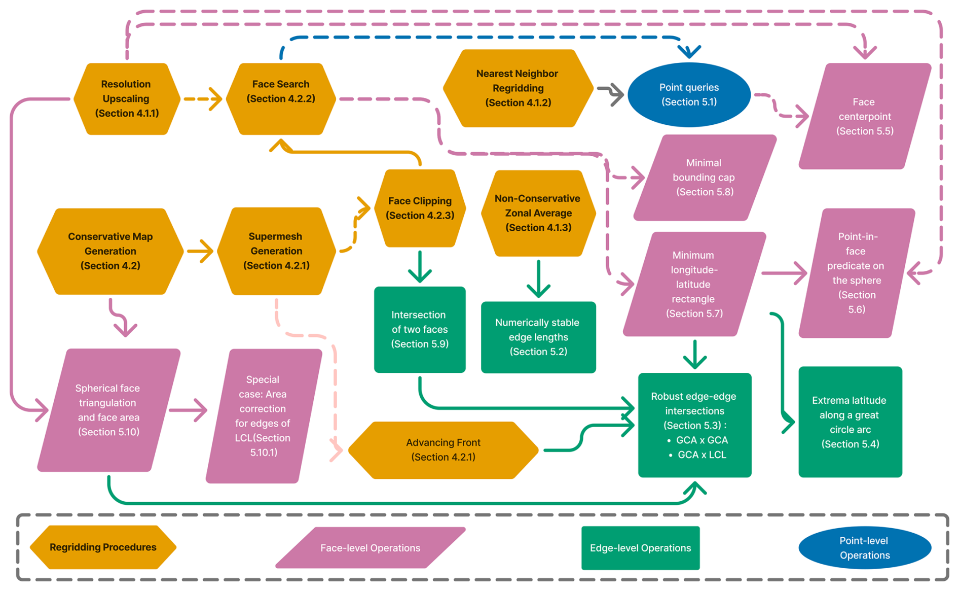
Figure 1 End-to-end workflow for the regridding and mesh-intersection procedures developed in this paper. Shapes indicate the level at which an operation is defined: circles represent point-level operations, rectangles represent edge-level operations, right-leaning parallelograms represent face-level operations, and hexagons represent multi-level regridding procedures. Within the light red blocks, bold text denotes complete, standalone steps in the regridding workflow, whereas non-bold text (e.g., the advancing-front procedure) indicates subcomponents that form part of a larger step, such as supermesh generation. Arrows indicate dependencies: A→B means that A depends on B. Solid (dashed) arrows denote required (optional) dependencies.

4.1 Non-conservative map generation

4.1.1 Resolution upscaling

Resolution upscaling refers to the transfer of data from a finer grid to a coarser grid, as discussed in Sect. 3.4. In some cases, the fine grid is generated by subdividing a coarser grid, making each coarse cell the parent of several fine cells and storing this parent-child relationship directly in the data structure, as in S2 Geometry and HEALPix. In such cases, upscaling is straightforward because the set of fine-grid faces contained in each coarse face is known from the grid hierarchy. If a conservative scheme is desired, the elements of the linear map along each row are simply determined by the fractional area contribution of the child cell to its parent (Sect. 5.10). However, non-conservative methods, e.g., simply averaging the data values from all child nodes found in a parent region, are also common in practice.

When this hierarchical information is not available, upscaling requires determining which fine-grid faces lie inside each coarse-grid face. A common strategy is to compute the face centerpoints for all source (fine) faces using Sect. 5.5, then apply the point-in-face predicate from Sect. 5.6 to test whether each fine-grid centerpoint lies within a coarse-grid cell. To accelerate this process and avoid testing against all coarse faces, spatial indexing methods from Sect. 5.1 can be used to pre-filter candidate coarse cells before performing the more expensive containment checks.

4.1.2 Nearest-neighbor regridding

Nearest-neighbor regridding assigns each target face the value of the nearest source face, based on the centerpoints defined in Sect. 5.5. This produces a local, monotone, and widely used non-conservative mapping suitable for categorical variables, masks, and quick-look diagnostics. To perform geometric nearest-neighbor search procedures, one can use the methods described in Sect. 5.1; Sect. 4.2.2 shows how the same search tools also serve as a filtering step for overlap detection in conservative workflows. The resulting sparse matrix representation of the nearest neighbor operator is purely binary (consisting of only 1 and 0 s) with exactly one 1 per row.

4.1.3 Non-conservative zonal averaging

Zonal averaging can be viewed as a special case of regridding, with the target grid consisting of LCLs or bands. Non-conservative zonal averaging replaces area weighting with a purely geometric length weighting along a chosen LCL. For a prescribed latitude ϕ₀, each face intersected by the parallel contributes to the zonal average in proportion to the length of the segment cut out by that parallel. This procedure requires only the intersection of each face with a constant-latitude line and its associated segment length calculation, using the techniques introduced in Sect. 5.2 and 5.3. No face areas or overlap polygons are used.

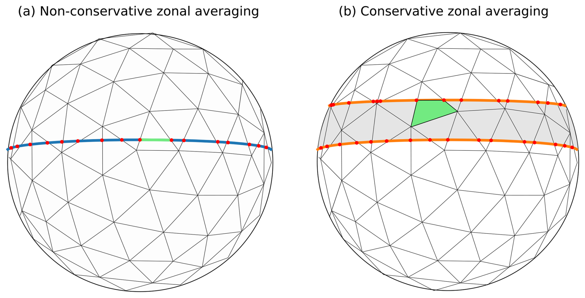
Figure 2 Comparison between (a) non-conservative and (b) conservative zonal averaging on an unstructured spherical mesh. In the non-conservative case, the weight contributed by each face is the length of the constant-latitude segment lying inside the face (green segment). In the conservative case, the weight is the spherical area of the overlap between the face and the zonal band (green polygon). The red points mark face-parallel intersection nodes, and the shaded regions in panel (b) illustrate the finite-width zonal band used for conservative averaging.

4.2 Conservative map generation

4.2.1 Supermesh generation

Two approaches are commonly employed for generating supermeshes: global advancing-front arrangement and a local tree-based search-and-clip strategy.

General computational-geometry workflows based on global advancing-front mesh arrangements insert all source and target edges into a single arrangement structure, eliminating the need for an explicit search procedure. As detailed in Sect. 5.9, each edge is inserted on the sphere, while the arrangement algorithm detects and processes edge-edge intersections using the intersection kernels from Sect. 5.3, creates any new intersection vertices, and updates the arrangement graph. Once this global arrangement is built, geometric queries such as point-in-face tests (Sect. 5.6), retrieval of intersecting faces, and extraction of clipped overlap polygons (Sect. 5.9) reduce to direct lookups from the arrangement data structure. Thus, the advancing-front method automatically resolves the face-pair discovery step.

Tree-based search-and-clip methods provide an alternative approach that can avoid explicit construction of the global supermesh. These methods identify only those face pairs that may overlap, using bounding volumes from Sect. 5.7 and Sect. 5.8, along with the face search from Sect. 4.2.2 and face clipping from Sect. 4.2.3. The resulting approach computes exactly the overlap region needed for conservative regridding while retaining scalability. State-of-the-art implementations of this strategy appear in TempestRemap and YAC.

4.2.2 Face search

Face search identifies pairs of faces from two meshes that may overlap. By iterating over the faces of one mesh and querying the other, face search produces a set of candidate source-target face pairs that may overlap and so builds the supermesh through iteration. Three techniques are commonly employed for face search: nearest-neighbor queries based on face centerpoints, minimum bounding caps, and minimum longitude-latitude rectangles combined with interval trees. These filtering techniques reduce the number of face pairs that must be processed by the exact clipping routines.

If nearest-neighbor queries are used, face centerpoints must first be computed using one of the techniques described in Sect. 5.5. Methods from Sect. 5.1 can then be applied to guarantee all overlaps are found by conditioning the queries on the sum of the maximum radius of the bounding circle around that center point from the source and target meshes. However, such an operation could also provide a large number of false positives if grid cells are distorted.

Bounding spherical caps attached to each grid face are used by YAC to perform candidate face filtering, as described in Sect. 5.8. YAC distributes work across MPI processes using an internal spatial domain decomposition constructed as a binary tree over all grid vertices via recursive great-circle splits, analogous to a spherical k–d tree. This approach avoids ambiguity and yields a consistent and well-balanced spatial partitioning. For each process, the grid faces associated with its subdomain are equipped with bounding spherical caps (Sect. 5.8), which are organized in a similar tree structure. First, all subdomains whose spatial extent overlaps the bounding spherical cap of the query face are identified. Second, within each selected subdomain, potentially overlapping source-face caps are retrieved from the local tree. Both stages are performed analogously to k–d tree range queries. For each candidate pair, overlap is assessed by checking whether the great-circle distance between the cap centers does not exceed the sum of their angular radii. The numerically stable great circle arc distance formula is introduced in Sect. 5.2. Face pairs passing this filter are subsequently processed by the exact face-clipping routine introduced in Sect. 4.2.3, which produces the geometric overlap information required for conservative weight generation. The resulting overlap areas are sufficient for first-order schemes, while higher-order schemes require additional geometric moments such as barycenters, as discussed in later sections. The worst-case computational complexity of this method is O(N_tN_s), where N_t and N_s denote the number of target and source faces, respectively. However, in practice, performance improvements come from spatial filtering and a balanced search tree indexing source circles, reducing the expected cost to O(N_tlog N_s+M), with M representing the total number of actual intersections (Hanke et al., 2016). Benchmark results on realistic production grids from Hanke et al. (2016) demonstrate that this method is more than twice as efficient as the bucket-based approaches currently used in the community.

A novel contribution of the current paper is the formal documentation of the bounding-rectangle (see Sect. 5.7) sweep-line algorithm used for spherical regridding. While this method has already been implemented in TempestRemap, it has not previously been described in the literature. The algorithm combines bounding rectangles with a sweep-line procedure and k–d trees, achieving $O\left(\right(N_{\mathrm{t}}+N_{\mathrm{s}}\left)\log \right(N_{\mathrm{t}}+N_{\mathrm{s}}\left)\right)$ complexity (Shamos and Hoey, 1976; Souvaine, 2008). In practice, the planar sweep-line algorithm is directly adapted to the sphere. To simplify calculations, the domain boundary is assumed to be aligned so that its left edge lies at zero longitude. The algorithm proceeds as follows:

• Calculate the bounding rectangles for all grid faces on both the source and target grids (as in Sect. 5.7).

• Initialize two interval trees, one for each of the source and target grids, to store the latitude intervals of active bounding rectangles during the longitude sweep. Bounding rectangles that cross the 0° meridian, i.e., those whose left boundary has a larger longitude value than the right boundary, are active at the start of the sweep and are therefore inserted into the corresponding interval tree during initialization. For each stored latitude interval, also record the associated grid face index.

• Construct a sorted array of left and right rectangle edges, ordered by increasing longitude and combining edges from both source and target grids. For each entry, store the latitude bounds of the rectangle, whether the edge belongs to the source or target grid, the index of the corresponding face, and whether the edge is a left or right boundary.

• Traverse the sorted array of rectangle edges. At each step, examine one edge e belonging to face c. If e is a left edge, insert the latitude interval of c into the interval tree corresponding to its grid. If e is a right edge, remove the latitude interval of c from the corresponding interval tree. When a left edge from the source grid is processed, check for overlaps between its latitude range and the active ranges in the target grid interval tree. Similarly, when a left edge from the target grid is processed, query the source interval tree. If an overlap is detected, the pair of faces $(c,c^{\prime })$ are marked as candidates, where c^′ is the face associated with the overlapping latitude range. If c contains the 0° meridian in its interior, then faces c^′ must be excluded if their left edges have longitude ≥0 but are positioned to the left of the right edge of c, since such pairs will already have been recorded when the left edge of c^′ was processed. After this filtering, valid pairs $(c,c^{\prime })$ are passed to the exact intersection routine in Sect. 5.9. Each overlapping pair is processed exactly once.

This bounding-rectangle approach is amenable to parallel execution, since source and target grids can be partitioned across multiple processors. Practical implementations handle overlaps across subdomain boundaries using standard techniques such as ghost regions or replicated search structures.

4.2.3 Face clipping

Once candidate face pairs are identified by one of the above searches, exact overlap polygons can be obtained by performing the face-face intersection and spherical clipping described in Sect. 5.9. This step produces the overlap polygons that form the cells of the supermesh. To get the overlap areas $J_{ij}^{\mathrm{ov}}$, a triangulation and area calculation procedure is usually needed (Sect. 5.10.1).

4.2.4 Conservative zonal average

The conservative zonal average is a special case of conservative regridding. To perform a conservative zonal average, we first define a subdivision of the latitude domain into bands $B_i=[{\mathit{\varphi }}_i,{\mathit{\varphi }}_{i+\mathrm{1}}]\times [\mathrm{0},\mathrm{2}\mathit{\pi }]$ for $i=\mathrm{0},\mathrm{\dots },N-\mathrm{1}$. Each band B_i is treated as a target grid cell. The constant-latitude boundaries ϕ=ϕ_i form a non-GCA, so care must be taken to compute overlap areas with the corrections described in Sect. 5.10.1. A critical consideration in zonal averaging is the precise geometric treatment of constant-latitude boundaries, as emphasized in Sect. 5.3. The accurate and efficient determination of intersection points, particularly involving constant-latitude lines, can be facilitated by the AccuX algorithm described in detail by Chen et al. (2026). Integrating these refined intersection and area-adjustment techniques into the general area-weighted regridding methodology thus provides a straightforward approach to achieving accurate and conservative zonal averages.

5 Low-level geometry on the sphere

We now describe the low-level algorithmic kernels that underlie the high-level operations described in the previous section, with the aim of providing sufficient detail to enable any regridding package developer to reproduce these operations.

5.1 Node-level: Point-based proximity queries

Point-based proximity queries include operations such as nearest-neighbor search, k-nearest neighbors, and fixed-radius search, which are used to identify candidate nodes or other mesh entities associated with a given query point. In practice, higher-level entities such as faces are often represented by point surrogates (e.g., face centroids) for the purpose of these queries. Such proximity searches form an essential component of many spatial indexing and tree-based algorithms. These tasks rely on data structures that balance query speed, memory usage, and implementation complexity.

A common strategy for performing efficient point-based proximity queries is to organize points into bounding-volume hierarchies, which integrate naturally into a variety of search structures (e.g., k–d trees or ball trees). This approach groups points into regions enclosed by simple bounding shapes, such as spheres, axis-aligned boxes, oriented boxes, geodesic rectangles, or spherical caps. These structures guarantee O(log N) expected query time with O(N) storage, although the constants depend strongly on how tightly the bounding volumes fit the data. Simpler shapes are cheaper to construct and maintain but allow more false positives, while tighter shapes prune more aggressively at higher preprocessing cost.

A standard approach is to embed spherical nodes into ℝ³ and construct a k–d tree (TempestRemap). Despite relying on Euclidean chord distances, nearest-neighbor correctness is preserved because chord distance and great-circle distance induce identical neighbor orderings. Balanced k–d trees have O(Nlog N) build time, O(log N) average query time, and linear storage, though axis-aligned splits may yield suboptimal pruning for spherical distributions.

Ball trees avoid Euclidean embedding altogether. Each node encloses its points within a spherical radius, and all computations use exact great-circle distances. This can improve pruning behavior for certain point sets. UXarray, for example, employs BallTree queries with the haversine metric on latitude-longitude coordinates.

Other metric trees, such as cover trees, also guarantee logarithmic query complexity with linear storage and support exact great-circle distances, though in practice they are often slower than k–d or ball trees in low dimensions. YAC employs a spherical variant of a binary space partitioning tree, where each split is defined by a great-circle plane through the origin.

Hash-grids are a novel approach for partitioning the domain into uniform bins, giving O(1) expected query time for small search radii but degrading toward linear complexity as the radius grows. However, this favorable behavior relies on a roughly uniform point density across bins. Sparse hash tables are typically used to retain O(N) storage in global settings. The GriSPy library provides a Python implementation of fixed-radius nearest-neighbor search based on this approach. In their paper (Chalela et al., 2021), the authors compare its performance with cKDTree in SciPy (Virtanen et al., 2020) and BallTree in scikit-learn. They find that for moderate-sized datasets (up to about 10⁷ points), tree-based methods are faster, while beyond roughly 10⁷ points, GriSPy becomes more efficient. For very large datasets (≳ 10⁸ points), its scaling is more favorable, as the query time grows more slowly with N compared to tree-based structures. Although grid construction introduces an initial cost, the grid can be reused for repeated queries, making the overhead negligible. Overall, hash-grid methods are particularly suitable for large, static datasets that require many nearest-neighbor queries on the same data, but are not currently implemented in any presently-available regridding package.

In practice, k–d trees and ball trees offer broadly similar asymptotic performance, with actual efficiency determined by implementation quality and hardware optimization. Both sklearn.neighbors.BallTree and sklearn.neighbors.KDTree are benchmarked in Sect. S5 for reference. Figures S7 and S8 show that KDTree construction is moderately slower, with build times typically within a factor of ∼ 1.5–2 of BallTree at large node counts. In contrast, KDTree queries are consistently faster by approximately one order of magnitude (about 10×) across all tested configurations. Smaller leaf sizes further accelerate queries, and the resulting increase in build time becomes negligible at large node counts.

5.2 Edge-level: Numerically stable edge lengths

For a GCA on the unit sphere, the length of the arc is given by the central angle Δσ between its endpoints x₁ and x₂. This angle is simply the angle between the two unit vectors drawn from the sphere’s center to the endpoints. In practice, Δσ can be computed using several equivalent trigonometric forms, for example,

$$\begin{array}{}\text{(9)}& \begin{array}{rl}& \mathrm{\Delta }{\mathit{\sigma }}_{\mathrm{asin}}=\arcsin \left(\Vert {\mathit{x}}_{\mathrm{1}}\times {\mathit{x}}_{\mathrm{2}}\Vert \right),\\ & \mathrm{\Delta }{\mathit{\sigma }}_{\mathrm{acos}}=\arccos \left({\mathit{x}}_{\mathrm{1}}\cdot {\mathit{x}}_{\mathrm{2}}\right),\\ & \mathrm{\Delta }{\mathit{\sigma }}_{\mathrm{atan}}=\mathrm{atan}\mathrm{2}\left(\Vert {\mathit{x}}_{\mathrm{1}}\times {\mathit{x}}_{\mathrm{2}}{\Vert }_{\mathrm{2}},{\mathit{x}}_{\mathrm{1}}\cdot {\mathit{x}}_{\mathrm{2}}\right).\end{array}\end{array}$$

Shewchuk (2013) analyzes the accuracy and failure modes of cosine-, sine-, and tangent-based formulas when they are used within geometric predicates and constructions. Knyazev and Argentati (2002) provides an overview of the sine and cosine accuracy behavior over small and large angles and proposes an algorithm to switch between them to maintain a high accuracy. Kahan (2006) considers these issues from a numerical analysis perspective, highlighting the limitations of both the sine and cosine formulas and recommending a more robust alternative. While Kahan's formula was originally expressed in terms of arctan, we express it here in terms of the standard library function atan2 and simplify to the following expression (using the fact that x₁ and x₂ are both unit vectors):

$$\begin{array}{}\text{(10)}& \mathrm{\Delta }{\mathit{\sigma }}_{\mathrm{Kahan}}=\mathrm{2}\mathrm{atan}\mathrm{2}\left({∥{\mathit{x}}_{\mathrm{1}}-{\mathit{x}}_{\mathrm{2}}∥}_{\mathrm{2}},{∥{\mathit{x}}_{\mathrm{1}}+{\mathit{x}}_{\mathrm{2}}∥}_{\mathrm{2}}\right).\end{array}$$

Kahan's formulation mitigates precision loss in near-degenerate configurations. In Sect. S5, we benchmark the relative errors of several trigonometric formulations. Kahan’s method achieves relative errors on the order of a small multiple of the machine epsilon of the floating-point system u (approximately 10⁻¹⁵ in double precision), with no measurable computational overhead. In contrast, alternative formulations exhibit substantial degradation in ill-conditioned configurations, with errors increasing by several orders of magnitude (ranging from approximately 10⁻¹¹ up to 10⁻³ in double precision, depending on the baseline angle). We therefore recommend this approach for edge-length computations.

For the LCL case, if we let the endpoints ${\mathit{x}}_{\mathrm{1}}=(x_{\mathrm{1}},y_{\mathrm{1}},z_{\mathrm{0}})$ and ${\mathit{x}}_{\mathrm{2}}=(x_{\mathrm{2}},y_{\mathrm{2}},z_{\mathrm{0}})$ lie on the unit sphere in the plane z=z₀, then the longitude span Δλ can be obtained from Kahan's angle formula applied on a constant z-plane, which simplifies to:

$$\begin{array}{rl}\mathrm{\Delta }\mathit{\lambda }& =\mathrm{2}\mathrm{atan}\mathrm{2}\left(\sqrt{(x_{\mathrm{1}}-x_{\mathrm{2}}{)}^{\mathrm{2}}+(y_{\mathrm{1}}-y_{\mathrm{2}}{)}^{\mathrm{2}}},\right.\\ & \left.\sqrt{(x_{\mathrm{1}}+x_{\mathrm{2}}{)}^{\mathrm{2}}+(y_{\mathrm{1}}+y_{\mathrm{2}}{)}^{\mathrm{2}}}\right).\end{array}$$

The longitude span then translates into edge length via

$$\begin{array}{}\text{(11)}& \begin{array}{rl}& r=\sqrt{\mathrm{1}-z_{\mathrm{0}}^{\mathrm{2}}}=\sqrt{x_{\mathrm{1}}^{\mathrm{2}}+y_{\mathrm{1}}^{\mathrm{2}}}=\sqrt{x_{\mathrm{2}}^{\mathrm{2}}+y_{\mathrm{2}}^{\mathrm{2}}},\\ & \mathrm{\Delta }{s}_{z_{\mathrm{0}}}=r\mathrm{\Delta }\mathit{\lambda }=\sqrt{\mathrm{1}-z_{\mathrm{0}}^{\mathrm{2}}}\mathrm{\Delta }\mathit{\lambda }.\end{array}\end{array}$$

This formulation is valid for $\left|\mathrm{\Delta }\mathit{\lambda }\right|\le \mathit{\pi }$; if $(x_{\mathrm{1}},y_{\mathrm{1}})=-(x_{\mathrm{2}},y_{\mathrm{2}})$ then Δλ=π.

5.3 Edge-level: Robust edge-edge intersections

The intersection of grid lines is one of the most important geometry subproblems for regridding. Since LCLs cannot intersect one another, there are only two canonical cases: the intersection of (1) two great circle arcs, or (2) a great circle arc and a LCL.

5.3.1 Case 1: GCA-GCA intersection

The intersection points v_± of great circle arcs $({\mathit{x}}_{\mathrm{1}}^{\mathrm{1}},{\mathit{x}}_{\mathrm{2}}^{\mathrm{1}})$ and $({\mathit{x}}_{\mathrm{1}}^{\mathrm{2}},{\mathit{x}}_{\mathrm{2}}^{\mathrm{2}})$ are given by

$$\begin{array}{}\text{(12)}& \stackrel{\mathrm{̃}}{\mathit{v}}=({\mathit{x}}_{\mathrm{1}}^{\mathrm{1}}\times {\mathit{x}}_{\mathrm{2}}^{\mathrm{1}})\times ({\mathit{x}}_{\mathrm{1}}^{\mathrm{2}}\times {\mathit{x}}_{\mathrm{2}}^{\mathrm{2}}),{\mathit{v}}_{\pm }=\pm {\displaystyle \frac{\stackrel{\mathrm{̃}}{\mathit{v}}}{\Vert \stackrel{\mathrm{̃}}{\mathit{v}}\Vert }}.\end{array}$$

However, direct evaluation of these formulae in floating-point arithmetic can introduce round-off error, so the resulting great-circle plane normals may deviate slightly from the true perpendicular to the arc's plane. A widely used remedy is to evaluate each cross-product entry with Kahan's 2 × 2 determinant, often referred to as the difference of products algorithm (Higham, 2002; Jeannerod et al., 2013). This algorithm relies on fused multiply-add (FMA) instructions that were first implemented for the IBM RISC System/6000 architecture (Hokenek et al., 1990; Montoye et al., 1990). The underlying FMA kernels and their use in accurate discriminant evaluation are described in Kahan (2006, 2004), and Jeannerod et al. (2013) derives tight error bounds for this difference of products algorithm. Such implementations of FMA-based cross-product can be found in UXarray, as well as in YAC and, through code integration, in CDO, where they substantially reduce intersection error on geodesic grids.

Error-free transformations (EFTs) can be used here to further improve the accuracy of the great-circle plane normal vector computations and the resulting intersection point. We introduce a novel and accurate cross-product computation, obtained by chaining EFT primitives (Chen et al., 2026; Ogita et al., 2005) into a compensated cross product, AccuCross (described as Algorithm A1 in Appendix A). This kernel is subsequently used in the more accurate intersection calculation, AccuXGCA, and presented as Algorithm A2 in Appendix A, which consists of two successive calls to AccuCross followed by an EFT-based normalization that incorporates the accurate square root AccuSqrt from Rump (2023).

We also provide a detailed analytical error analysis of AccuCross and AccuXGCA in Sect. S1 in the Supplement. For AccuCross, the final relative error is bounded by O(u²), as shown in Eq. (S2).

For AccuXGCA, the analysis distinguishes two asymptotic regimes based on the magnitude of the subexpression $|\stackrel{\mathrm{̃}}{\mathit{v}}{|}^{\mathrm{2}}$. In both regimes, the leading-order term of the relative error remains O(u). In contrast, the direct floating-point implementation exhibits an error bound of $O\left(\sqrt{u}\right)$, indicating a loss of approximately half of the working precision.

These analytical bounds are confirmed by empirical accuracy assessments in Sect. S5.2, where we compare against two float64 implementations: (i) direct evaluation and (ii) evaluation using Kahan’s 2 × 2 determinant with FMA. The test consists of 200 000 randomly generated samples concentrated near ill-conditioned configurations.

Both the analytical and empirical results show that for nondegenerate inputs, AccuXGCA achieves errors near machine precision, and for all cases it effectively matches the accuracy of evaluating the same expressions at approximately twice the working precision and then rounding back to the target precision, without measurable performance overhead.

5.3.2 Case 2: GCA-LCL intersection

Intersecting a GCA with a LCL poses additional numerical challenges, especially in near-tangent scenarios. Among current geoscience libraries, only YAC – and by extension, CDO and UXarray – explicitly handle this computation. YAC computes this intersection using a formulation combining FMA operations to reduce rounding errors. A comprehensive review by Chen et al. (2026), including detailed benchmarks, evaluates the numerical properties of YAC's approach and proposes a more numerically robust alternative, given by Eq. (13), where the unnormalized normal vector n of the plane containing the GCA and its horizontal projection n_xy are defined as

$$\mathit{n}={\mathit{x}}_{\mathrm{1}}\times {\mathit{x}}_{\mathrm{2}}=(n_x,n_y,n_z{)}^{\mathsf{T}},{\mathit{n}}_{xy}=(n_x,n_y{)}^{\mathsf{T}}.$$

The segment intersects the parallel z=z₀ provided $\Vert {\mathit{n}}_{xy}{\Vert }_{\mathrm{2}}^{\mathrm{2}}\ge \Vert \mathit{n}{\Vert }_{\mathrm{2}}^{\mathrm{2}}{z}_{\mathrm{0}}^{\mathrm{2}}$, with equality indicating tangency. The two antipodal intersection points are then given by

$$\begin{array}{}\text{(13)}& {\mathbf{P}}_{\pm }=\left[\begin{array}{c}-\frac{z_{\mathrm{0}}{n}_x{n}_z\pm s{n}_y}{\Vert {\mathit{n}}_{xy}{\Vert }_{\mathrm{2}}^{\mathrm{2}}}\\ -\frac{z_{\mathrm{0}}{n}_y{n}_z\mp s{n}_x}{\Vert {\mathit{n}}_{xy}{\Vert }_{\mathrm{2}}^{\mathrm{2}}}\\ z_{\mathrm{0}}\end{array}\right],s=\sqrt{\Vert {\mathit{n}}_{xy}{\Vert }_{\mathrm{2}}^{\mathrm{2}}-\Vert \mathit{n}{\Vert }_{\mathrm{2}}^{\mathrm{2}}{z}_{\mathrm{0}}^{\mathrm{2}}}.\end{array}$$

The direct implementation of Eq. (13) is already incorporated in UXarray. When evaluated with the EFT-based AccuX algorithm of Chen et al. (2026), the intersection calculations are improved to near machine precision. Importantly, this higher accuracy is achieved with essentially the same runtime as the direct method when batch-processed on a parallel system.

Our AccuSphGeom package provides SIMD-accelerated implementations of AccuX and AccuXGCA with batch-processing APIs.

5.4 Edge-level: Extrema latitude along a great circle arc

Planar intuition dictates that extrema of longitude and latitude lie at polygon vertices, and many packages adopt this shortcut by constructing bounding boxes solely from vertex coordinates. On the sphere, however, the maximum latitude of a GCA may occur along the arc, and neglecting this case can misrepresent bounding boxes and compromise downstream geometric operations. Many existing geoscience packages, such as ESMF and its MBMesh variant with MOAB's AABB methods, continue to rely exclusively on vertex extrema and are therefore susceptible to this approximation error.

In this work, we present a formula for the extremal latitude along a GCA. It was first implemented in TempestRemap and is documented here for the first time. Following the parameterization of a GCA introduced in Sect. 2 and defined in Eq. (3), let $a\in [\mathrm{0},\mathrm{1}]$ denote the interpolation parameter. defining z(a) as the z-coordinate of the corresponding point along the arc, we we find from Eq. (3) that

$$z\left(a\right)={\displaystyle \frac{(\mathrm{1}-a)z_{\mathrm{1}}+a{z}_{\mathrm{2}}}{\parallel (\mathrm{1}-a){\mathit{x}}_{\mathrm{1}}+a{\mathit{x}}_{\mathrm{2}}{\parallel }_{\mathrm{2}}}}.$$

The maximum latitude along the arc occurs either at the endpoints ($a=\mathrm{0},\mathrm{1}$) or at an interior point where $\partial z/\partial a=\mathrm{0}$, which leads to

$$a={\displaystyle \frac{z_{\mathrm{1}}({\mathit{x}}_{\mathrm{1}}\cdot {\mathit{x}}_{\mathrm{2}})-z_{\mathrm{2}}}{(z_{\mathrm{1}}+z_{\mathrm{2}})({\mathit{x}}_{\mathrm{1}}\cdot {\mathit{x}}_{\mathrm{2}}-\mathrm{1})}}.$$

Only if $a\in (\mathrm{0},\mathrm{1})$ does the extremum lie within the arc. In that case, the latitude of the extremal point ϕ_max is

$$\begin{array}{}\text{(14)}& {\mathit{\varphi }}_{\max }=\arcsin \left(z_{\max }\right)=\arcsin \left[{\displaystyle \frac{\mathrm{2}{z}_{\mathrm{1}}{z}_{\mathrm{2}}({\mathit{x}}_{\mathrm{1}}\cdot {\mathit{x}}_{\mathrm{2}})-z_{\mathrm{1}}^{\mathrm{2}}-z_{\mathrm{2}}^{\mathrm{2}}}{(z_{\mathrm{1}}+z_{\mathrm{2}})({\mathit{x}}_{\mathrm{1}}\cdot {\mathit{x}}_{\mathrm{2}}-\mathrm{1})}}\right].\end{array}$$

5.5 Face-level: Face centerpoint

Face centerpoints are useful for sampling of fields or for use in nearest-neighbor operations. On latitude-longitude meshes, the centerpoint of each face is usually taken to be the arithmetic mean of the latitude and longitude bounds, performed in latitude-longitude space. However, on unstructured grids, the specific definition used for the “centerpoint” often varies across models and software packages. In practice, the particular choice of centerpoint usually has minimal effect on subsequent applications (e.g., through point queries), but there is value in documenting these different choices. Four approaches are commonly employed for the centerpoint:

• Nodal Average. The simplest approach for obtaining a centerpoint uses the average of the Cartesian coordinates of the vertices of the face, projected to the surface of the sphere. While this approach may be desirable for its simplicity, it is only sensible to employ it for simple polygons with roughly equally spaced vertices. For instance, splitting an edge into two via vertex insertion will move the centroid towards that edge despite no change in the shape of the face. Despite its shortcomings, this approach is currently used in UXarray and TempestRemap.

• Centroid. Letting M⊂𝕊² denote a face, its spherical area is $A={\int }_M\mathrm{d}A$ and its first moment is $\mathbf{M}={\int }_M\mathit{x}\mathrm{d}A$. The true three-dimensional centroid is $\mathit{c}=\mathbf{M}/A$, which lies on the interior of the unit sphere. The centroid is then defined by mapping c back to the sphere, obtaining $\widehat{\mathit{c}}=\mathbf{M}/\Vert \mathbf{M}{\Vert }_{\mathrm{2}}$.

Let ${\mathit{x}}_{\mathrm{1}},{\mathit{x}}_{\mathrm{2}},{\mathit{x}}_{\mathrm{3}}\in {\mathbb{R}}^{\mathrm{3}}$ be unit vectors to the vertices of a spherical triangle with area A. Combining the three-dimensional centroid formulas of Brock (1975) with the stable interior angle expression in Eq. (10), we define for any oriented edge (a,b) the following functions:

$$\begin{array}{}\text{(15)}& \widehat{\mathit{n}}(\mathit{a},\mathit{b})={\displaystyle \frac{\mathit{a}\times \mathit{b}}{\Vert \mathit{a}\times \mathit{b}{\Vert }_{\mathrm{2}}}},\text{and}\mathit{\alpha }(\mathit{a},\mathit{b})=\mathrm{2}\mathrm{atan}\mathrm{2}\left(\Vert \mathit{a}-\mathit{b}{\Vert }_{\mathrm{2}},\Vert \mathit{a}+\mathit{b}{\Vert }_{\mathrm{2}}\right).\end{array}$$

Then the centroid is

$$\begin{array}{}\text{(16)}& \begin{array}{rl}\mathit{c}& ={\displaystyle \frac{\mathrm{1}}{\mathrm{2}A}}\left[\widehat{\mathit{n}}\right({\mathit{x}}_{\mathrm{1}},{\mathit{x}}_{\mathrm{2}}\left)\mathit{\alpha }\right({\mathit{x}}_{\mathrm{1}},{\mathit{x}}_{\mathrm{2}})+\widehat{\mathit{n}}({\mathit{x}}_{\mathrm{2}},{\mathit{x}}_{\mathrm{3}}\left)\mathit{\alpha }\right({\mathit{x}}_{\mathrm{2}},{\mathit{x}}_{\mathrm{3}})\\ & +\widehat{\mathit{n}}({\mathit{x}}_{\mathrm{3}},{\mathit{x}}_{\mathrm{1}})\mathit{\alpha }({\mathit{x}}_{\mathrm{3}},{\mathit{x}}_{\mathrm{1}})].\end{array}\end{array}$$

For a general face on the unit sphere without self-intersection, let each constituent spherical triangle have true centroid c_i and spherical area A_i. Also let the face boundary be given by m vertices in counterclockwise order ${\mathit{v}}_{\mathrm{1}},{\mathit{v}}_{\mathrm{2}},\mathrm{\dots },{\mathit{v}}_m$ with wraparound ${\mathit{v}}_{m+\mathrm{1}}\equiv {\mathit{v}}_{\mathrm{1}}$. Interior edges cancel in any triangulation by antisymmetry of the oriented edge contributions in Eq. (16). Combined with $\mathbf{M}={\sum }_i{A}_i{\mathit{c}}_i$, the total first moment depends only on the boundary walk

$$\begin{array}{}\text{(17)}& \mathbf{M}={\displaystyle \frac{\mathrm{1}}{\mathrm{2}}}\sum _{k=\mathrm{1}}^m\widehat{\mathit{n}}({\mathit{v}}_k,{\mathit{v}}_{k+\mathrm{1}})\mathit{\alpha }({\mathit{v}}_k,{\mathit{v}}_{k+\mathrm{1}}).\end{array}$$

Thus, the centroid of the face can be obtained by $\mathit{c}=\mathbf{M}/A$ and $\widehat{\mathit{c}}=\mathbf{M}/\Vert \mathbf{M}\Vert$.

Equivalently, Eq. (17) can be obtained by applying Stokes' theorem on the unit sphere, which relates the surface first moment to a boundary integral that collapses to an edge sum for geodesic polygonal boundaries (Alexandrov, 2002; Jones, 2002, Chap. 13, Prob. 13–12).

Note that Eq. (17) is valid only for faces whose boundary consists entirely of great-circle arcs. If a boundary edge lies on a LCL, Eq. (17) requires a correction analogous to the area adjustment in Sect. 5.10.1. We decompose the moment into a great-circle contribution and a correction strip,

$$\begin{array}{}\text{(18)}& \mathbf{M}=\sum _{k=\mathrm{1}}^m\widehat{\mathit{n}}({\mathit{v}}_k,{\mathit{v}}_{k+\mathrm{1}})\mathit{\alpha }({\mathit{v}}_k,{\mathit{v}}_{k+\mathrm{1}})+{\mathbf{M}}_{\mathrm{corr}}({\mathit{\varphi }}_{\mathrm{0}},\mathrm{\Delta }\mathit{\lambda }),\end{array}$$

where (ϕ₀,Δλ) describe the constant-latitude edge.

For a single edge along ϕ=ϕ₀ with endpoints at longitudes λ₁=0 and λ₂=Δλ, the correction region is the strip between the parallel ϕ=ϕ₀ and the great-circle arc joining its endpoints. Denoting by $\stackrel{\mathrm{̃}}{\mathit{\varphi }}\left(\mathit{\lambda }\right)$ the latitude of this arc at longitude λ, the corresponding first moment is provided below

$$\begin{array}{}\text{(19)}& \begin{array}{rl}{\mathbf{M}}_{\mathrm{corr}}({\mathit{\varphi }}_{\mathrm{0}},\mathrm{\Delta }\mathit{\lambda })& =\underset{\mathrm{0}}{\overset{\mathrm{\Delta }\mathit{\lambda }}{\int }}\underset{{\mathit{\varphi }}_{\mathrm{0}}}{\overset{\stackrel{\mathrm{̃}}{\mathit{\varphi }}\left(\mathit{\lambda }\right)}{\int }}\mathit{x}(\mathit{\varphi },\mathit{\lambda })\cos \mathit{\varphi }\mathrm{d}\mathit{\varphi }\mathrm{d}\mathit{\lambda }\\ & =\underset{\mathrm{0}}{\overset{\mathrm{\Delta }\mathit{\lambda }}{\int }}{\mathbf{M}}_{\mathrm{inner}}\left(\mathit{\lambda }\right)\mathrm{d}\mathit{\lambda },\end{array}\end{array}$$

Summing M_corr over all constant-latitude edges and adding the great-circle boundary contributions yields the first moment for any spherical polygon with mixed great-circle and constant-latitude segments. In Sect. S2 we derive an exact integral representation for the inner moment M_inner(λ), reducing the correction term to a single one-dimensional integral in λ (see Eq. S5). While this reduced integral does not admit a simple closed-form antiderivative, it can be evaluated efficiently using numerical quadrature.

For a more accurate floating-point implementation, all cross and dot products in this expression should employ the adapted EFT-fused cross products introduced in this work (Algorithm A1), together with the adapted EFT-fused and composable dot product and normalization schemes proposed by Chen et al. (2026).

• Intersection of Geodesic Diagonals or Bimedians. For spherical quadrilaterals, geodesic diagonals connect opposing vertices of each face, while bimedians connect the centerpoints of each edge. The intersection of those lines can then be used as a polygonal centerpoint. This approach echoes the planar convention of using diagonal intersections (Willmott et al., 1985). For small, nearly convex cells, this construction is close to both the area centroid and the mid-latitude/mid-longitude center, consistent with the local planarity of small regions on the sphere (Snyder, 1987).

• Center of the Minimum Bounding Circle. The minimum bounding circle is the smallest circle on the sphere that includes all vertices of the spherical polygon (discussed further in section Sect. 5.8). Welzl's algorithm, which applies in Cartesian geometry, can be readily extended to spherical geometry for this application (Flemming, 2024a). This approach is implemented in UXarray as an alternative centerpoint calculation and may be desirable because of its relationship with the minimum bounding circle and insensitivity to vertex density.

5.6 Face-level: Point-in-face predicate on the sphere

Point-in-face tests determine whether a query point lies inside, outside, or on the boundary of a face, but rely purely on edge-level geometry. Such predicates are among the most frequently invoked geometric tests in spherical regridding, for example when determining whether a given cell includes the pole point, or whether a particular point should contribute to a face in a non-conservative resolution upscaling method.

As emphasized by Schirra (1997), the robustness of point-query tests is governed by the accuracy of their geometric building blocks. In particular, when a query point lies near the boundary of a face, the computation is highly sensitive to the accuracy of the edge geometry – especially the intersection points produced in Sect. 5.3. Any round-off introduced at this stage propagates directly into the sign evaluations that underpin point-in-face logic; hence the high-accuracy kernels mentioned in Sect. 5.3 are an essential prerequisite for robust implementations.

The most widely used on-the-fly method for point-in-face is ray casting: a great-circle ray is emitted from the query point x_Q in a fixed direction towards a target point known to be outside the face, and the algorithm counts how many times this ray intersects the polygon edges. An odd number of crossings indicates that the point is inside, and an even number indicates that it is outside (Bevis and Chatelain, 1989). If a face is constrained to a single hemisphere (Sect. 2.3), then the antipodal point of the sample point suffices as the target.

Note that this method does not require explicitly computing the intersection points between the ray and each edge – simply knowing whether or not they intersect is sufficient. In more general computational geometry packages, these crossings are typically detected using orientation predicates such as Orient3D (Shewchuk, 1997), which avoid the need for explicit geometric intersection computations. Because they rely only on the sign of a scalar triple product, orientation predicates are more efficient and more numerically stable. The predicate $\mathrm{Orient}\mathrm{3}\mathrm{D}(\mathit{A},\mathit{B},\mathit{O},\mathit{Q})$ returns the sign of the oriented volume $\left(\left(\mathit{A}-\mathit{O})\times (\mathit{B}-\mathit{O})\right)\cdot (\mathit{Q}-\mathit{O}\right)$, indicating whether the point Q lies on the positive or negative side of the oriented plane defined by A, B, and the origin O, with zero indicating coplanarity.

Let $\mathit{A},\mathit{B},\mathit{C},\mathit{D}\in {\mathbb{S}}^{\mathrm{2}}$ denote the endpoints of two minor arcs AB and CD. Each oriented arc induces an oriented great-circle plane through the origin O, partitioning the sphere into a positive and a negative open hemisphere. Accordingly, the sign of $\mathrm{Orient}\mathrm{3}\mathrm{D}(\mathit{A},\mathit{B},\mathit{O},\mathit{X})$ determines on which side of the plane ABO a point X lies, and similarly $\mathrm{Orient}\mathrm{3}\mathrm{D}(\mathit{C},\mathit{D},\mathit{O},\mathit{X})$ with respect to the plane CDO. The two great circles defined by AB and CD intersect at exactly two antipodal points. If the two minor arcs intersect, the intersection must occur at one of these two points, as illustrated in Fig. 3. These two possibilities correspond to the same endpoint sign pattern up to a global sign flip. This yields a symmetric crossing criterion: the arcs AB and CD intersect if and only if the following orientation relations hold:

$$\begin{array}{}\text{(20)}& \begin{array}{rl}& \mathrm{Orient}\mathrm{3}\mathrm{D}(\mathit{C},\mathit{D},\mathit{O},\mathit{A})=\mathrm{Orient}\mathrm{3}\mathrm{D}(\mathit{A},\mathit{B},\mathit{O},\mathit{D})=\\ & -\mathrm{Orient}\mathrm{3}\mathrm{D}(\mathit{A},\mathit{B},\mathit{O},\mathit{C})=-\mathrm{Orient}\mathrm{3}\mathrm{D}(\mathit{C},\mathit{D},\mathit{O},\mathit{B}).\end{array}\end{array}$$

Equivalently, the signs associated with endpoints A and D agree, the signs associated with B and C agree, and these two groups have opposite sign. This predicate-based intersection test has been implemented in the S2 Geometry library (S2 Geometry Developers, 2025), which additionally applies early-exit filters to efficiently reject certain clearly non-intersecting cases before evaluating all predicates.

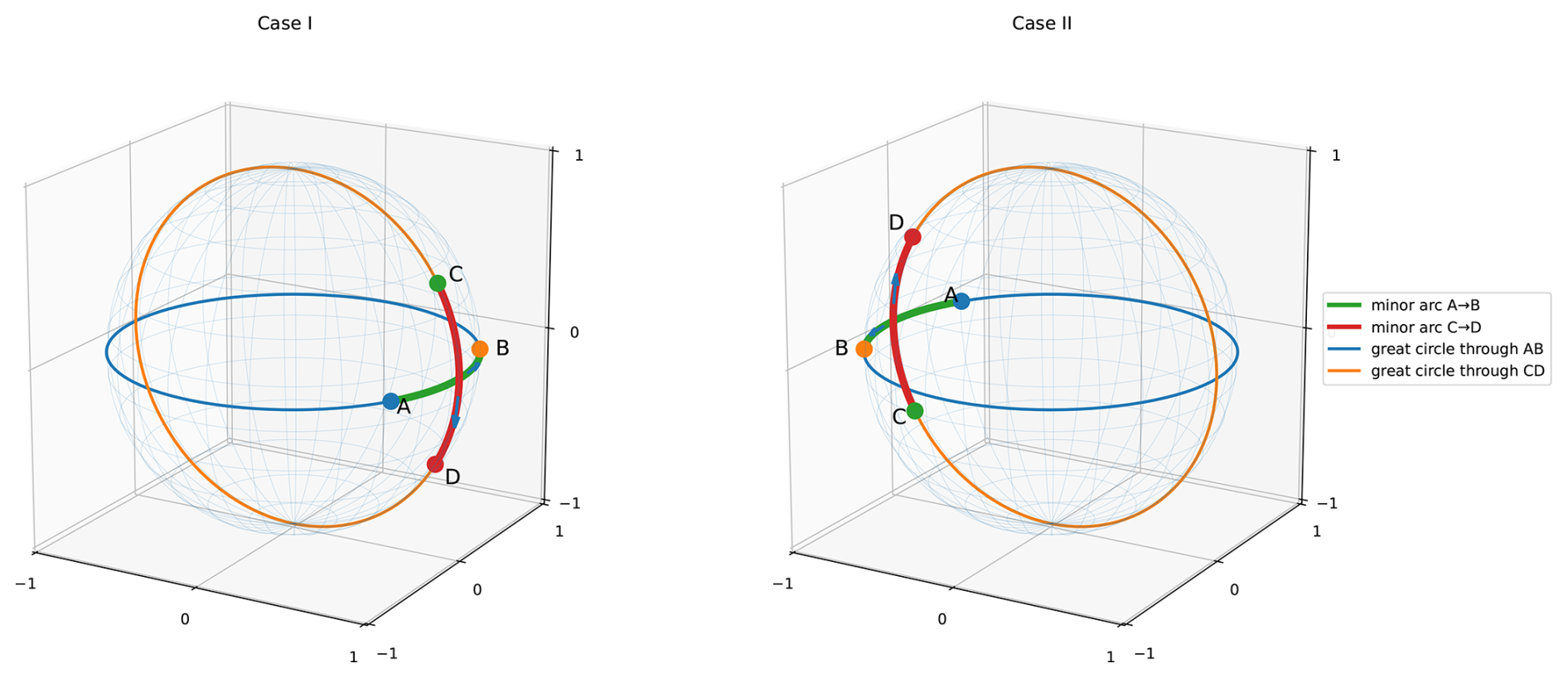
Figure 3 The two possible arc intersection cases (left and right). In the configuration on the left, the orientation predicates evaluate to $\mathrm{Orient}\mathrm{3}\mathrm{D}(\mathit{A},\mathit{B},\mathit{O},\mathit{C})=+\mathrm{1}$, $\mathrm{Orient}\mathrm{3}\mathrm{D}(\mathit{A},\mathit{B},\mathit{O},\mathit{D})=-\mathrm{1}$, $\mathrm{Orient}\mathrm{3}\mathrm{D}(\mathit{C},\mathit{D},\mathit{O},\mathit{A})=-\mathrm{1}$, and $\mathrm{Orient}\mathrm{3}\mathrm{D}(\mathit{C},\mathit{D},\mathit{O},\mathit{B})=+\mathrm{1}$. For the configuration on the right, all signs are reversed: $\mathrm{Orient}\mathrm{3}\mathrm{D}(\mathit{A},\mathit{B},\mathit{O},\mathit{C})=-\mathrm{1}$, $\mathrm{Orient}\mathrm{3}\mathrm{D}(\mathit{A},\mathit{B},\mathit{O},\mathit{D})=+\mathrm{1}$, $\mathrm{Orient}\mathrm{3}\mathrm{D}(\mathit{C},\mathit{D},\mathit{O},\mathit{A})=+\mathrm{1}$, and $\mathrm{Orient}\mathrm{3}\mathrm{D}(\mathit{C},\mathit{D},\mathit{O},\mathit{B})=-\mathrm{1}$.

By contrast, most geoscientific packages implement ray casting via explicit intersection-point computations. Both orientation-based methods and explicit intersection-point approaches must address degeneracies, such as rays passing exactly through a vertex or becoming collinear with an edge, which are discussed later in this subsection.

Again, if each spherical face occupies less than a complete hemisphere, the spherical point-in-polygon problem reduces to the planar version, as proven in Li and Sun (2026). Once degeneracies are addressed, the core ray-casting procedure proceeds as follows:

1. For a given face, consider the query point x_Q whose containment status is to be determined.

2. Select the antipodal point of the query point, denoted x_OUT. Since each face spans less than a hemisphere (see Sect. 2), the face cannot contain both x_Q and x_OUT simultaneously.

3. Connect x_Q and x_OUT with a great-circle arc interval, chosen according to the implementation. Count the number of intersections between this arc and the edges of the face. If the count is odd, x_Q lies inside the face; if even, it lies outside.

In floating-point arithmetic, the 3D orientation predicate $\mathrm{Orient}\mathrm{3}\mathrm{D}(\mathit{A},\mathit{B},\mathit{O},\mathit{Q})$ can be evaluated reliably in most cases without requiring exact arithmetic. When all points are provided explicitly as input, and the origin is fixed at $\mathit{O}=[\mathrm{0},\mathrm{0},\mathrm{0}]$, the predicate simplifies to computing the scalar triple product $(\mathit{A}\times \mathit{B})\cdot \mathit{Q}$. This determinant can be evaluated in standard double precision along with a certified upper bound on its round-off error.

Let $\mathit{A}=[a_x,a_y,a_z]$, $\mathit{B}=[b_x,b_y,b_z]$, and $\mathit{Q}=[q_x,q_y,q_z]$ denote input points with floating-point coordinates. Following the analysis of Shewchuk (1997), the error in computing $(\mathit{A}\times \mathit{B})\cdot \mathit{Q}$ is bounded in terms of the permanent P:

$$\begin{array}{}\text{(21)}& \begin{array}{rl}P& =\left|a_x\right|\left(\right|b_y{q}_z|+|b_z{q}_y\left|\right)+\left|a_y\right|\left(\right|b_z{q}_x|+|b_x{q}_z\left|\right)\\ & +\left|a_z\right|\left(\right|b_x{q}_y|+|b_y{q}_x\left|\right).\end{array}\end{array}$$

The absolute round-off error in evaluating the determinant E_det is then bounded by:

$$\begin{array}{}\text{(22)}& \left|E_{\text{det}}\right|\le (\mathrm{7}+\mathrm{56}\mathit{\epsilon })\mathit{\epsilon }P,\end{array}$$

where ε denotes the unit roundoff for the working floating-point format; for IEEE double precision, $\mathit{\epsilon }={\mathrm{2}}^{-\mathrm{53}}$ (IEEE, 2008). This error bound yields a floating-point filter for the orientation predicate: the scalar triple product is computed in floating point, and its magnitude is compared against the bound (7+56ε)εP. If the computed value exceeds this bound, the sign is guaranteed to be correct; otherwise, the computation escalates to higher precision.

The bound itself may be applied in two modes: a static filter assumes that all coordinates are bounded in magnitude by a known constant M, yielding the worst-case estimate P≤6M³; for inputs on the unit sphere, M=1, leading to the global bound $\left|E_{\text{det}}\right|\le \mathrm{6}(\mathrm{7}+\mathrm{56}\mathit{\epsilon })\mathit{\epsilon }$. In contrast, a semi-static filter computes P directly from the actual coordinate values, yielding tighter bounds and avoiding unnecessary escalation while preserving robustness (Shewchuk, 1997; Attene, 2020).

As shown by Shewchuk (1997), for double-precision inputs the initial floating-point evaluation succeeds in nearly all non-degenerate configurations. Escalation to exact arithmetic is only required near true degeneracies. This approach, arithmetic filtering with exact fallback, underlies the robust predicate kernels used in computational geometry libraries such as CGAL, ensuring correctness while maintaining high performance (Attene, 2020).

When predicates depend on intermediate constructions (e.g., applying Orient3D to points obtained from intersection calculations), standard filtering may fail or require frequent escalation and recalculation of the construction. To improve performance while remaining fully robust, Attene (2020) introduces indirect predicates, which algebraically rewrite the predicate in terms of the original input primitives, bypassing explicit intermediate constructions. These methods combine semi-static filtering, dynamic interval filtering when necessary, and finally exact expansion arithmetic. Because the input data type is known, it is possible to determine in advance the precision required to evaluate a given determinant exactly. If the determinant is evaluated at this guaranteed precision and still yields zero, the configuration is known to be exactly degenerate. Such degeneracies can be handled in several ways, for example by switching to an alternate ray direction that avoids a small neighborhood around all vertices, or by applying explicit degeneracy-handling rules such as those described in Hormann and Agathos (2001) to prevent double counting. Simulation of Simplicity (SoS) (Edelsbrunner and Mücke, 1990) handles exact degeneracies by symbolically perturbing the input by an infinitesimal amount, allowing degenerate configurations to be treated as if they were in general position while leaving all nondegenerate relationships unchanged. The S2 Geometry library adopts this framework through its RobustCrossing and VertexCrossing routines (S2 Geometry Developers, 2025), which rely on indirect predicates and Simulation of Simplicity to robustly handle the degeneracies described above. Finally, the EFT kernels introduced in Sect. 5.3 can be applied in practice to further improve performance while maintaining accuracy by refining the precision of intermediate coordinates and reducing the number of cases that require escalation to higher-precision determinant evaluation.

Another commonly used and closely related on-the-fly technique for point-in-face testing is based on traveling the winding number, which measures how many times the face winds around the query point P_Q; a point is outside the face only if this value is zero and inside otherwise (Hormann and Agathos, 2001). It can be computed using the incremental-angle algorithm of Weiler (1994), though this approach is computationally expensive due to its reliance on trigonometric and square-root evaluations. As shown in Hormann and Agathos (2001), the incremental-angle formulation can be rewritten as a ray-crossing test, demonstrating that the winding-number and even-odd rules are equivalent in principle. As with ray-casting, winding-number evaluation relies on orientation predicates to determine the relative position of the query point with respect to each edge. The winding-number method is topologically invariant and naturally accommodates arbitrary face configurations, including self-intersections and faces with holes. However, for the class of faces defined in Sect. 2, which are uniform and free of self-intersections, as is typical in geoscientific meshes, the winding-number test reduces directly to the ray-casting even-odd rule.

If one maintains the data structure from the global advancing-front arrangement described in Sects. 3.2 and 4.2.1, the face overlay and point-location information are resolved automatically. As noted in CGAL's documentation (Wein et al., 2024), arrangement-based and on-the-fly methods represent complementary trade-offs: arrangement-based methods incur substantial preprocessing cost but enable fast point-location queries thereafter, whereas on-the-fly methods require no preprocessing but may be slower per query and must explicitly handle degeneracies.

We provide a C$++$ implementation of the point-in-face algorithm, including Simulation of Simplicity (SoS) handling, in the AccuSphGeom package.

5.7 Face-level: Minimum longitude-latitude rectangle

Bounding boxes in longitude-latitude coordinates provide an efficient geometric filter for candidate face-face intersections on the sphere, particularly in combination with interval trees. If faces only consist of lines of constant latitude and longitude then such rectangles are easy to construct, but if faces also consist of GCAs then the problem is non-trivial because of the curvature of the edges. Some additional care is needed to ensure the spherical geometry is handled correctly: for instance, longitudes 0 and 360° denote the same meridian, yet a naïve min/max calculation would treat them as maximally distant; additionally, near the poles, all longitudes converge to a single point, so longitudinal differences no longer reflect meaningful spatial separation. Only a few libraries, such as TempestRemap and its MPI-parallel variant mbtempest and UXarray, correctly construct spherical bounding rectangles.

A valid minimum longitude-latitude rectangle can be constructed in three main steps:

1. Determine the maximum latitude of each face using the procedure described in Sect. 5.4.

2. Apply the pole-in-face test from Sect. 5.6. If the north (south) pole lies within the face, the bounding rectangle spans all longitudes, and only the minimum (maximum) latitude defines its vertical extent.

3. Otherwise, compute the minimal longitude interval that bounds the face boundary under the chosen periodic longitude convention. If this interval does not cross the periodic longitude cut, it is represented as a single half-open interval. If it crosses the periodic cut, the interval is split into two half-open intervals on either side of the cut, both associated with the same face identifier. This representation is used when inserting bounding rectangles into the interval-tree structures required by Sect. 4.2.2.

In contrast with the strategy above, ESMF employs a hybrid strategy combining bounding spheres with axis-aligned bounding boxes (AABBs). An AABB is the smallest Cartesian box that encloses all vertex coordinates, obtained from their component-wise minima and maxima. However, because ESMF only considers the vertex positions and ignores the curvature of the spherical surface, it may miss the true extrema in latitude. A bounding sphere is then computed, centered at the cell centroid, with radius equal to the maximum distance from the centroid to any AABB corner. This guarantees no overlaps are missed but admits more false positives than TempestRemap's tighter gnomonic-projection boxes, increasing cost at high resolution. Despite this overhead, ESMF achieves comparable remapping accuracy to TempestRemap in terms of global conservation and field interpolation error, particularly when using its second-order conservative option, although its performance is more sensitive to grid uniformity and convexity assumptions (Mahadevan et al., 2022).

Our AccuSphGeom package provides a C$++$ vectorized implementation of the longitude-latitude bounds computations, including pole-region handling.

5.8 Face-level: Minimal bounding cap (spherical circle)

As introduced in Sect. 5.5, the minimal bounding circle is the smallest spherical bounding cap enclosing all face vertices, defined by a center and angular radius. When a face is composed exclusively of GCAs, spherical convexity guarantees that a cap containing all vertices also contains the entire face interior. This property follows from classical results on geodesic convexity on the sphere (Naszódi, 2018; Fricke, 2006; Flemming, 2024a). In this setting, representing a face by its minimal bounding cap provides a compact and robust bound that naturally accommodates anti-meridian crossings and faces containing a pole, and this approach is adopted in YAC.

On the plane, the most widely used algorithm to compute the smallest enclosing circle for a set of points is Welzl's algorithm (Welzl, 1991). This recursive algorithm has an average-case time complexity of O(n). One can adapt Welzl's approach to the sphere by using great-circle distances instead of Euclidean distances, and this has been done by YAC and UXarray. However, this substitution is heuristic: Welzl's correctness proof is Euclidean, so merely replacing the distance with a great‐circle metric does not guarantee the returned spherical bounding cap is truly minimal, especially for large hemispherical point sets. Recently, Flemming (2024a) presented a linear-time algorithm on the sphere that extends Welzl's procedure: it maintains the current minimal cap as points are added and automatically checks whether the set so far still fits in a hemisphere. If the points are hemisphere-bounded, the algorithm finds the exact smallest enclosing cap in linear time. If not, one must resort to more complex methods for the full-sphere case. An implementation of Flemming's spherical algorithm is available in open-source code (Flemming, 2024b), making it practical for geoscience libraries to adopt.

The correctness proofs for Welzl's algorithm and its spherical extension rely on a property specific to geodesic distance: if two points lie inside a spherical cap, then the shorter GCA between them lies entirely inside that cap. Since the cap boundary intersects any great circle in at most two points, the cap interior corresponds to a single connected interval along that circle. This property does not extend to faces with LCL edges selected by a “shortest-in-longitude” convention, for which the chosen arc need not coincide with the portion of the latitude circle contained within the cap; in particular, when the cap center lies in the angular region opposite an LCL edge, the farthest point from the center may occur along the LCL, at the point whose longitude differs by 180° from that of the center. As a result, an edge may exit the cap even when all vertices are contained. This additional point along the LCL should then be included as an additional vertex when computing the radius of the bounding cap.

5.9 Face-level: Intersection of two faces

Face overlay, which is also referred to as face clipping or face intersection, identifies overlapping regions between two faces, creating new faces that represent these intersections (Martínez et al., 2009). This task has been extensively studied in planar geometry, where a variety of efficient algorithms exist (Foley et al., 1990). Among them, the Sutherland–Hodgman algorithm (Sutherland and Hodgman, 1974) is notable for its simplicity and efficiency, iteratively clipping a face against each edge of a convex or rectangular window. However, Sutherland-Hodgman assumes planar clipping, so applying it on the sphere requires custom great-circle intersection and inside-outside tests. Other algorithms address these limitations: the Weiler–Atherton method (Weiler and Atherton, 1977) supports general faces with holes but requires complex data structures; Vatti's algorithm (Vatti, 1992) is more flexible but complex, leveraging a sweep-line technique; and the Greiner–Hormann algorithm (Greiner and Hormann, 1998), although simpler, handles degeneracies through perturbation. More recently, Martínez et al. (2009) recast plane-sweep clipping so that every new edge intersection is immediately split, reducing the event queue to simple left/right endpoints and yielding higher throughput than Vatti on large planar faces.

Extending planar clipping algorithms to spherical geometries introduces additional complexities, especially when face edges include both GCAs and constant-latitude lines. As discussed in Sect. 3, spherical face clipping can be achieved through mesh arrangements on spherical surfaces. The framework of Cazals and Loriot (2009), originally developed for arrangements of circles on parametric surfaces, can be adapted to arrangements of arc intervals on the sphere rather than full circles. In this context, planar intersection detection techniques – most notably the Bentley–Ottmann sweep-line algorithm (Bentley and Ottmann, 1979) – are extended to spherical surfaces. A half-edge data structure supports efficient handling of intersections among spherical arc segments, with clipped faces generated directly during the arrangement construction. In CGAL, this method is implemented within the 2D Arrangements package, which provides arrangements embedded on the sphere (Wein et al., 2024). Although CGAL's kernel can represent general circles in 3D (de Castro et al., 2024; Castro et al., 2009), the spherical arrangement code explicitly supports only GCAs. Exact arithmetic is employed throughout to guarantee robustness of the overlay construction (Wein et al., 2024; de Castro et al., 2024; Castro et al., 2009).

Grid faces from traditional geoscientific models typically have uniform shape, do not self-intersect, have no internal holes, and span significantly less than 180°. Given these conditions, simpler clipping methods generally suffice. Consequently, TempestRemap and UXarray directly adopt the planar Sutherland–Hodgman algorithm, assuming purely great-circle face edges. Extending this slightly further, YAC supports clipping between longitude-latitude grids (containing constant-latitude edges) and great-circle face grids by employing a specialized spherical edge-intersection routine. YAC triangulates the clipping face into spherical triangles and then applies Sutherland–Hodgman clipping with signed area accumulation. Although YAC handles these two specific face types effectively, it does not yet support faces composed of mixed edge types.

For highly irregular grids such as watershed-derived faces, significant gaps remain. Mainstream GIS libraries such as GEOS (GEOS contributors, 2025) do not natively support spherical polygon clipping and instead interpret latitude-longitude coordinates as planar, which is acceptable for small regions but breaks down for global-scale shapes or polygons spanning hemispheres. Watershed boundaries derived from DEMs (for example via TauDEM, Tarboton, 2016, 1997 or HydroSHEDS, Lehner et al., 2021) are typically produced as complex planar polygons in geographic coordinates. These tools focus on basin delineation rather than spherical overlay, so any spherical clipping or triangulation, such as intersecting watershed faces with a model grid or computing their spherical areas, must be handled by downstream GIS or climate-modeling tools. Climate remapping frameworks can process many of these polygons at a functional level, but numerical robustness remains limited, particularly in floating-point-sensitive cases such as near-degenerate edge intersections.

Computational geometry frameworks can achieve robust clipping using exact arithmetic, as in CGAL's 2D Arrangements, but typically at the cost of performance. S2 Geometry, as detailed before in Sect. 3.4, utilizes snap rounding to avoid precision error. This approach is well-suited to GIS applications. However, compared to an EFT-based direct intersection scheme, S2's snap-rounded, lattice-based representation sacrifices exact spherical geometry and strict area conservation in favor of topological robustness, which makes it unsuitable for high-accuracy conservative remapping where arc shapes, intersection points, and cell areas must be preserved to near machine precision. Moreover, S2's hierarchical, topology-centric data structures and reliance on integer arithmetic hinder effective vectorization on modern CPU and GPU architectures.

5.10 Face-level: Spherical face triangulation and face area

The area of a spherical face is typically computed by first subdividing the face into spherical triangles and then summing their individual areas. For convex or mildly concave faces, two triangulation strategies are commonly used in geoscience software: the centerpoint approach and the vertex fan approach. The centerpoint approach, used in more recent versions of TempestRemap, computes a face centerpoint (see Sect. 5.5) and forms triangles using the centerpoint together with each consecutive edge of the face. This approach is illustrated in Fig. 4. The vertex fan approach, implemented in YAC and ESMF, instead fixes a single vertex and forms triangles between that vertex and each consecutive edge of the face. This latter approach may produce more elongated triangles than the centerpoint approach, but doesn't require an additional centerpoint calculation. The vertex fan approach is illustrated in Fig. 5.

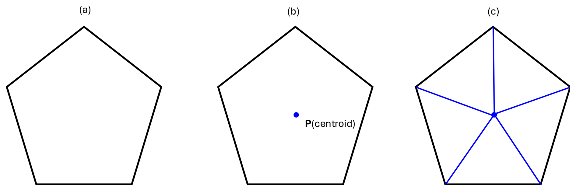
Figure 4 Starting with the face shown in (a), we first compute its centroid as illustrated in (b). Using this centroid, we then form a fan triangulation by connecting the centroid to each pair of consecutive vertices of the face, as shown in (c).

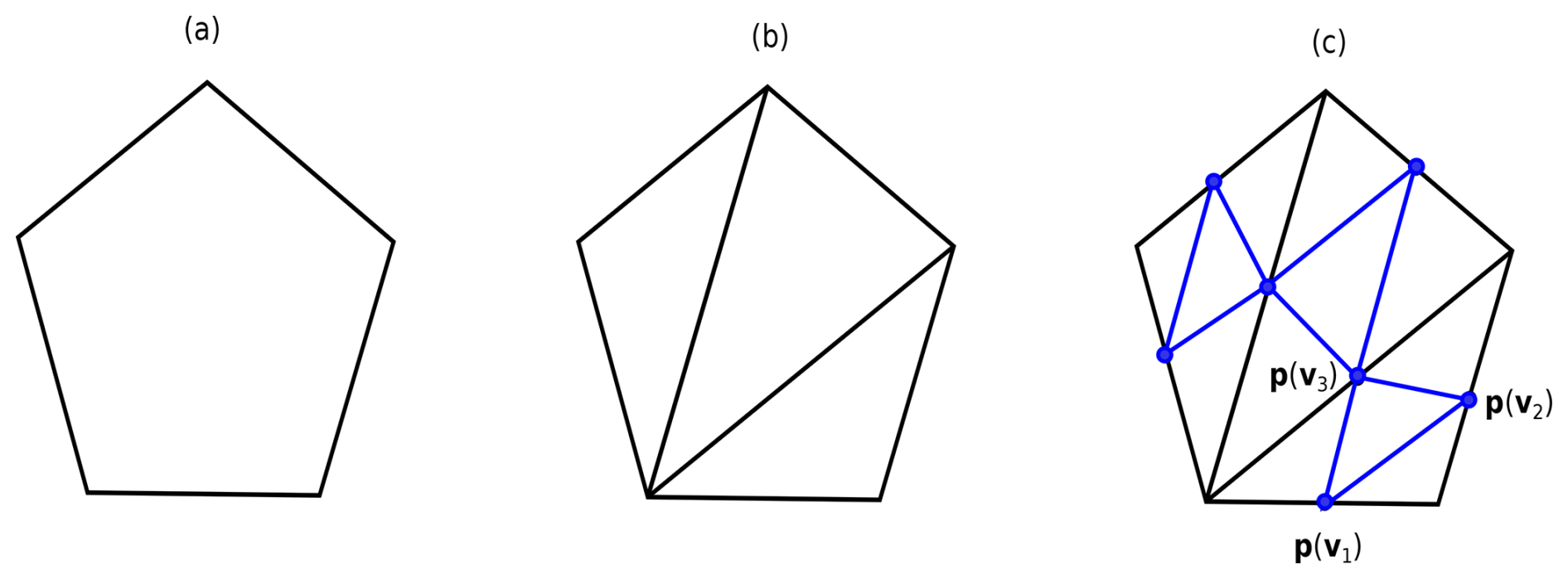
Figure 5 Starting with the face in (a), we divide it into sub-triangular faces as in (b). Given a sub-triangle in (b), we subdivide it into another four triangles by connecting the points p(v₁), p(v₂), and p(v₃).

Once the face has been decomposed into spherical triangles, their areas are computed. It is common to use formulae based on spherical excess E, which is equivalent to the area of a spherical triangle on the unit sphere. By definition, E is the sum of angles of a spherical triangle minus π (Girard's theorem; Girard, 1629), but this formula is not used in practice since it requires one to take the difference of two nearly equal quantities, leading to large cancellation errors. Instead, both ESMF and YAC use the algebraic L'Huilier formula (L’Huilier, 1784), which improves numerical stability for nearly degenerate or high aspect ratio triangles (Hanke et al., 2016).

A related formula for the spherical excess, discovered in the writing of this paper and due to Eriksson (1990), provides superior numerical performance but is not widely used. Let ${\mathit{x}}_{\mathrm{1}},{\mathit{x}}_{\mathrm{2}},{\mathit{x}}_{\mathrm{3}}\in {\mathbb{R}}^{\mathrm{3}}$ be unit vectors from the sphere center to the triangle vertices. Then the spherical excess E can be computed via a numerically stable atan2 call:

$$\begin{array}{}\text{(23)}& \begin{array}{rl}E& =\mathrm{2}\mathrm{atan}\mathrm{2}\left(|{\mathit{x}}_{\mathrm{1}}\cdot ({\mathit{x}}_{\mathrm{2}}\times {\mathit{x}}_{\mathrm{3}}\left)\right|,\mathrm{1}+{\mathit{x}}_{\mathrm{2}}\cdot {\mathit{x}}_{\mathrm{3}}+{\mathit{x}}_{\mathrm{3}}\cdot {\mathit{x}}_{\mathrm{1}}\right.\\ & \left.+{\mathit{x}}_{\mathrm{1}}\cdot {\mathit{x}}_{\mathrm{2}}\right)\end{array}\end{array}$$

which yields improved accuracy and requires fewer trigonometric evaluations than classical formulations. Although this expression is used internally in the spherical geometry utilities of Atlas (Deconinck et al., 2017), conservative and grid-box-average remapping operators are not yet supported. As a result, this formulation has not been benchmarked, analyzed, or exercised in the context of spherical polygon area evaluation or conservative weight construction within Atlas.

Quadrature-based methods are more complicated but can be more accurate than the L'Huilier formula because they avoid ill-conditioned trigonometric combinations. Quadrature-based methods can be improved by imposing a suitable bound on the face size and edge length, and splitting faces when the bound is exceeded. This approach is described in Sect. S3, and is used in TempestRemap. Anchored Radially Projected Integration on Spherical Triangles (ARPIST) (Li and Jiao, 2023) attains accurate and numerically stable integration by a radial-projection framework whose anchoring step mitigates the cancellation that can arise in direct Gaussian quadrature. One downside of quadrature-based methods is that because areas are computed over the interior of the face, numerical errors may result in the global mesh area deviating from 4π.

To assess the relative performance of these face-area formulations, we benchmark in Sect. S5 the improved Gaussian quadrature in ARPIST, the direct quadrature in TempestRemap, the L’Huilier-based implementation in YAC, and the closed-form expression in Eq. (23) derived from Eriksson (1990). As noted in Li and Jiao (2023) and confirmed by our results, the L’Huilier formulation is sensitive to triangles with extremely small edges or sharp angles, leading to numerical instability at high resolution. In such cases, its relative error can grow several orders of magnitude beyond the machine epsilon u (reaching approximately 10⁻⁵ in double precision).

Quadrature-based methods achieve relative errors on the order of 10³u (approximately 10⁻¹² in double precision), with accuracy improving as the number of quadrature points increases, at the cost of additional computation. In contrast, the Eriksson formulation maintains relative errors on the order of a small multiple of u (approximately 10⁻¹³ in double precision) across all tested resolutions.

Overall, the Eriksson formulation provides the best balance of accuracy and efficiency: as a closed-form geometric expression, it avoids the resolution-dependent cost of quadrature while maintaining near machine-precision accuracy. We therefore recommend it for general use. Augmenting it with error-free transformation (EFT) operators from Chen et al. (2026) may further improve accuracy without sacrificing performance; we leave this to future work.

For irregular or concave polygonal faces not typical of structured climate grids, such as watershed-derived faces, general spherical Delaunay triangulation methods can be applied in place of the simplified triangulation methods discussed above. In planar geometry, the widely-used Triangle library by Jonathan Shewchuk (Shewchuk, 1996) provides a robust option, producing high-quality triangulations (often Delaunay) through adaptive-precision arithmetic to ensure numerical robustness (Shewchuk, 1997). Extending planar triangulation methods to spherical geometry is commonly done by projecting small spherical regions onto tangent planes, applying planar triangulation there, and mapping the resulting mesh back onto the sphere. Alternatively, CGAL provides spherical Delaunay triangulations as described by Caroli et al. (2010). They note that floating-point number types cannot represent points lying exactly on the sphere, which undermines the orientation-based predicates required for Delaunay triangulation. To bridge this gap between theory and practice, Caroli et al. (2010) use a regular triangulation of weighted points: each 3D point is projected onto the sphere and assigned a weight based on its projection distance. They show that if the projected points remain sufficiently close to the sphere and sufficiently separated (for double precision, at least 2⁻²⁵r apart), then the regular triangulation of the weighted projected points coincides with the Delaunay triangulation of the original 3D points. If r is, for example, the radius of the Earth, roughly 6300 km, then this separation requirement is on the order of one meter.

For these highly irregular spherical faces, recent work by Chern and Ishida (2024) proposes an alternative approach that avoids triangulation entirely. Their method generalizes the planar Green’s theorem area formula to spherical polygons and remains robust for nearly degenerate edges and curves. Unlike classical Gauss-Bonnet-based formulations that rely on angle measurements, the prequantization-based construction applies to a broader class of degenerate spherical curves and polygons. This approach is very recent, and evaluating it in terms of performance, accuracy, and robustness for geoscience applications would make for interesting and valuable future work.

Special case: Area correction for edges of LCL

The area calculation discussed in the previous section only applies to spherical triangles composed of GCAs. If one edge of that triangle is instead an LCL, then an area adjustment is necessary to account for the slight differences in face area induced by the difference. In this section we provide a formula to account for that adjustment. The detailed derivation is provided in Sect. S4.

Without loss of generality, we can rotate the edge about the z axis so that x₁ and x₂ lie on the parallel ϕ=ϕ₀ with λ₁=0 and λ₂=Δλ:

$$\begin{array}{rl}& {\mathit{x}}_{\mathrm{1}}=(\cos {\mathit{\varphi }}_{\mathrm{0}},\mathrm{0},\sin {\mathit{\varphi }}_{\mathrm{0}}),\\ & {\mathit{x}}_{\mathrm{2}}=(\cos {\mathit{\varphi }}_{\mathrm{0}}\cos \mathrm{\Delta }\mathit{\lambda },\cos {\mathit{\varphi }}_{\mathrm{0}}\sin \mathrm{\Delta }\mathit{\lambda },\sin {\mathit{\varphi }}_{\mathrm{0}}).\end{array}$$

We consider the region bounded by the parallel ϕ=ϕ₀ and the GCA joining x₁ and x₂. In spherical geometry, the area of this region is given by:

$$\begin{array}{}\text{(24)}& A_{\mathrm{corr}}=\mathrm{2}\mathrm{atan}\mathrm{2}\left(\sin {\mathit{\varphi }}_{\mathrm{0}}\tan \left({\displaystyle \frac{\mathrm{\Delta }\mathit{\lambda }}{\mathrm{2}}}\right),\mathrm{1}\right)-\sin {\mathit{\varphi }}_{\mathrm{0}}\mathrm{\Delta }\mathit{\lambda },\end{array}$$

and in Cartesian geometry, in terms of the endpoints of this region, this function reads

$$\begin{array}{}\text{(25)}& \begin{array}{rl}{A}_{\mathrm{corr}}& =\mathrm{2}\mathrm{atan}\mathrm{2}\left(z(x_{\mathrm{1}}{y}_{\mathrm{2}}-x_{\mathrm{2}}{y}_{\mathrm{1}}),x_{\mathrm{1}}^{\mathrm{2}}+y_{\mathrm{1}}^{\mathrm{2}}+x_{\mathrm{1}}{x}_{\mathrm{2}}+y_{\mathrm{1}}{y}_{\mathrm{2}}\right)\\ & -z\mathrm{atan}\mathrm{2}\left(x_{\mathrm{1}}{y}_{\mathrm{2}}-x_{\mathrm{2}}{y}_{\mathrm{1}},x_{\mathrm{1}}{x}_{\mathrm{2}}+y_{\mathrm{1}}{y}_{\mathrm{2}}\right).\end{array}\end{array}$$

YAC also accounts for the mismatch between a GCA and an LCL edge, but adopts a different geometric construction. It forms a spherical triangle with vertices x₁, x₂, and the nearest pole. The resulting area discrepancy is the area correction, which is defined as $A_{\mathrm{corr}}=|A_{\mathrm{△}}^{\mathrm{GCA}}-A_{\mathrm{△}}^{\mathrm{LCL}}|,$ where $A_{\mathrm{△}}^{\mathrm{GCA}}$ denotes the area of this pole-endpoint triangle when all three edges are treated as great circle arcs, and $A_{\mathrm{△}}^{\mathrm{LCL}}$ denotes the area of the same triangle when only the edge between x₁ and x₂ is replaced by a line of constant latitude. When $A_{\mathrm{△}}^{\mathrm{GCA}}$ is evaluated using the accurate Eriksson formula (see Eq. 23), the resulting expression reduces to the closed-form LCL-GCA area difference given in Eq. (25).

6 Conclusions

This work presents a comprehensive overview of regridding algorithms from both a computational geometry and geoscientific modeling perspective. We begin by formalizing the geometric definitions essential to regridding, including accurate treatment of nodes, edges, and faces as used in climate modeling grids. Building on this foundation, we examine key geometric operations – including intersection detection and calculation, bounding region computation, face clipping, and area calculation – and review how these are handled across existing methods and software implementations.

These geometric primitives underpin the full regridding workflow, which we outline in detail. Particular attention is given to how prominent Earth system couplers and regridding tools – such as ESMF, YAC, TempestRemap, and its MPI-parallel variant mbtempest – implement these steps on the sphere. The discussion highlights the importance of precise geometric treatment, especially for edge cases like constant-latitude lines, which are increasingly relevant for high-accuracy and conservation-critical applications.

We aim to document the current state of implementation of these operations in geoscientific software and clarify how they relate to established methods in computational geometry. This resonates with recent calls in the community for more rigorous and reproducible handling of spherical geometry in regridding pipelines. While prior studies have benchmarked a range of regridding libraries, we note the absence of a direct comparison between YAC and TempestRemap/mbtempest – arguably the most geometry-aware and scalable regridding packages available today.

We therefore advocate for future benchmarking efforts that evaluate these (and other) tools side by side, in terms of both numerical accuracy and computational performance, especially in parallel settings. Such comparative studies will be instrumental for guiding the development and selection of robust, efficient, and physically consistent regridding strategies in next-generation Earth system models.

Appendix A: Algorithms

Algorithm A1 High-accuracy compensated cross product (AccuCross)

1:

Input: value/error pairs with ${\mathit{v}}_{\mathrm{1}},{\mathit{e}}_{v_{\mathrm{1}}},{\mathit{v}}_{\mathrm{2}},{\mathit{e}}_{v_{\mathrm{2}}}\in {\mathbb{F}}^{\mathrm{3}}$

2:

if ${\mathit{e}}_{v_{\mathrm{1}}}=\mathbf{0}$ and ${\mathit{e}}_{v_{\mathrm{2}}}=\mathbf{0}$ then

3:

$[{\widehat{v}}_{\mathrm{3}x},e_{{\widehat{v}}_{\mathrm{3}x}}]\leftarrow \mathtt{\text{AccuDOP}}\left({\mathit{v}}_{\mathrm{1}}\right[\mathrm{1}],{\mathit{v}}_{\mathrm{2}}[\mathrm{2}],{\mathit{v}}_{\mathrm{1}}[\mathrm{2}],{\mathit{v}}_{\mathrm{2}}[\mathrm{1}\left]\right)$

4:

$[{\widehat{v}}_{\mathrm{3}y},e_{{\widehat{v}}_{\mathrm{3}y}}]\leftarrow \mathtt{\text{AccuDOP}}\left({\mathit{v}}_{\mathrm{1}}\right[\mathrm{2}],{\mathit{v}}_{\mathrm{2}}[\mathrm{0}],{\mathit{v}}_{\mathrm{1}}[\mathrm{0}],{\mathit{v}}_{\mathrm{2}}[\mathrm{2}\left]\right)$

5:

$[{\widehat{v}}_{\mathrm{3}z},e_{{\widehat{v}}_{\mathrm{3}z}}]\leftarrow \mathtt{\text{AccuDOP}}\left({\mathit{v}}_{\mathrm{1}}\right[\mathrm{0}],{\mathit{v}}_{\mathrm{2}}[\mathrm{1}],{\mathit{v}}_{\mathrm{1}}[\mathrm{1}],{\mathit{v}}_{\mathrm{2}}[\mathrm{0}\left]\right)$

6:

else

7:

$[{\widehat{v}}_{\mathrm{3}x},e_{{\widehat{v}}_{\mathrm{3}x}}]\leftarrow \mathtt{\text{CompDotC}}\left(\begin{array}{l}[-e_{v_{\mathrm{1}}}[\mathrm{2}],e_{v_{\mathrm{1}}}[\mathrm{1}],v_{\mathrm{1}}[\mathrm{1}],-v_{\mathrm{1}}[\mathrm{2}],-e_{v_{\mathrm{1}}}[\mathrm{2}],v_{\mathrm{1}}[\mathrm{1}],e_{v_{\mathrm{1}}}[\mathrm{1}],-v_{\mathrm{1}}[\mathrm{2}\left]\right],\\ \left[e_{v_{\mathrm{2}}}\right[\mathrm{1}],e_{v_{\mathrm{2}}}[\mathrm{2}],e_{v_{\mathrm{2}}}[\mathrm{2}],e_{v_{\mathrm{2}}}[\mathrm{1}],v_{\mathrm{2}}[\mathrm{1}],v_{\mathrm{2}}[\mathrm{2}],v_{\mathrm{2}}[\mathrm{2}],v_{\mathrm{2}}[\mathrm{1}\left]\right]\end{array}\right)$

8:

$[{\widehat{v}}_{\mathrm{3}y},e_{{\widehat{v}}_{\mathrm{3}y}}]\leftarrow \mathtt{\text{CompDotC}}\left(\begin{array}{l}\left[e_{v_{\mathrm{1}}}\right[\mathrm{2}],-e_{v_{\mathrm{1}}}[\mathrm{0}],-v_{\mathrm{1}}[\mathrm{0}],v_{\mathrm{1}}[\mathrm{2}],e_{v_{\mathrm{1}}}[\mathrm{2}],v_{\mathrm{1}}[\mathrm{2}],-e_{v_{\mathrm{1}}}[\mathrm{0}],-v_{\mathrm{1}}[\mathrm{0}\left]\right],\\ \left[e_{v_{\mathrm{2}}}\right[\mathrm{0}],e_{v_{\mathrm{2}}}[\mathrm{2}],e_{v_{\mathrm{2}}}[\mathrm{2}],e_{v_{\mathrm{2}}}[\mathrm{0}],v_{\mathrm{2}}[\mathrm{0}],v_{\mathrm{2}}[\mathrm{2}],v_{\mathrm{2}}[\mathrm{2}],v_{\mathrm{2}}[\mathrm{0}\left]\right]\end{array}\right)$

9:

$[{\widehat{v}}_{\mathrm{3}z},e_{{\widehat{v}}_{\mathrm{3}z}}]\leftarrow \mathtt{\text{CompDotC}}\left(\begin{array}{l}[-e_{v_{\mathrm{1}}}[\mathrm{1}],e_{v_{\mathrm{1}}}[\mathrm{0}],v_{\mathrm{1}}[\mathrm{0}],-v_{\mathrm{1}}[\mathrm{1}],-e_{v_{\mathrm{1}}}[\mathrm{1}],v_{\mathrm{1}}[\mathrm{0}],e_{v_{\mathrm{1}}}[\mathrm{0}],-v_{\mathrm{1}}[\mathrm{1}\left]\right],\\ \left[e_{v_{\mathrm{2}}}\right[\mathrm{0}],e_{v_{\mathrm{2}}}[\mathrm{1}],e_{v_{\mathrm{2}}}[\mathrm{1}],e_{v_{\mathrm{2}}}[\mathrm{0}],v_{\mathrm{2}}[\mathrm{0}],v_{\mathrm{2}}[\mathrm{1}],v_{\mathrm{2}}[\mathrm{1}],v_{\mathrm{2}}[\mathrm{0}\left]\right]\end{array}\right)$

10:

end if

11:

Return: $({\mathit{v}}_{\mathrm{3}},{\mathit{e}}_{v_{\mathrm{3}}})$ with ${\mathit{v}}_{\mathrm{3}}=[{\widehat{v}}_{\mathrm{3}x},{\widehat{v}}_{\mathrm{3}y},{\widehat{v}}_{\mathrm{3}z}]$ and ${\mathit{e}}_{v_{\mathrm{3}}}=[e_{{\widehat{v}}_{\mathrm{3}x}},e_{{\widehat{v}}_{\mathrm{3}y}},e_{{\widehat{v}}_{\mathrm{3}z}}]$

Algorithm A2 Accurate great-circle intersection (AccuXGCA)

1:

Input: endpoints ${\mathit{x}}_{\mathrm{1}}^{\mathrm{1}},{\mathit{x}}_{\mathrm{2}}^{\mathrm{1}}$ and ${\mathit{x}}_{\mathrm{1}}^{\mathrm{2}},{\mathit{x}}_{\mathrm{2}}^{\mathrm{2}}\in {\mathbb{F}}^{\mathrm{3}}$

2:

$[{\mathit{n}}^{\mathrm{1}},e_{n^{\mathrm{1}}}]\leftarrow \mathtt{\text{AccuCross}}({\mathit{x}}_{\mathrm{1}}^{\mathrm{1}},\mathbf{0},{\mathit{x}}_{\mathrm{2}}^{\mathrm{1}},\mathbf{0})$

3:

$[{\mathit{n}}^{\mathrm{2}},e_{n^{\mathrm{2}}}]\leftarrow \mathtt{\text{AccuCross}}({\mathit{x}}_{\mathrm{1}}^{\mathrm{2}},\mathbf{0},{\mathit{x}}_{\mathrm{2}}^{\mathrm{2}},\mathbf{0})$

4:

$[\stackrel{\mathrm{̃}}{\mathit{v}},e_{\stackrel{\mathrm{̃}}{v}}]\leftarrow \mathtt{\text{AccuCross}}({\mathit{n}}^{\mathrm{1}},e_{n^{\mathrm{1}}},{\mathit{n}}^{\mathrm{2}},e_{n^{\mathrm{2}}})$

5:

$[N_{\mathrm{1}},n_{\mathrm{1}}]\leftarrow \mathtt{\text{SumOfSquaresC}}(\stackrel{\mathrm{̃}}{\mathit{v}},e_{\stackrel{\mathrm{̃}}{v}})$

6:

$[N_{\mathrm{2}},n_{\mathrm{2}}]\leftarrow \mathtt{\text{AccuSqrt}}(N_{\mathrm{1}},n_{\mathrm{1}})$

7:

$\mathit{v}\leftarrow \pm \frac{\stackrel{\mathrm{̃}}{\mathit{v}}}{N_{\mathrm{2}}}$

8:

Return: v

A key feature of AccuCross is its ability to incorporate compensated error terms for each input vector. This functionality allows the algorithm to address cases where the input data already contains known rounding errors, thereby ensuring robust performance. Such error handling is particularly important when the cross product is used as an intermediate step in more complex computations, where error accumulation could otherwise degrade overall accuracy.

One can also utilize the faithfully rounded Euclidean norm algorithm normNearest introduced in Rump (2023) and leave out the compensated term $e_{\stackrel{\mathrm{̃}}{v}}$ in AccuXGCA or extend the normNearest to accept compensated inputs through the same chaining strategy proposed in Chen et al. (2026). We will not pursue further exploration of such ideas here. Given the straightforward nature of these chained EFT operations, we omit extensive benchmarks here. However, future studies might provide detailed performance evaluations and analyses.