The new plant functional diversity model JeDi-BACH (version 1.0) in the ICON Earth System Model (version 1.0)

While it is clear that vegetation takes part in shaping terrestrial climate through various interactions with the atmosphere, it is not so obvious what role plant functional diversity plays here. So far a tool for investigating this question in land-atmosphere simulations was missing. The new tool JeDi-BACH (version 1.0), described here, closes this gap by combining the Jena Diversity Model (JeDi) with the land component JSBACHv4 of the ICON Earth System Model (version 1.0). In practice, the low-diversity plant parametrization of JSBACH employing plant functional types (PFTs) was replaced by the trait based high-diversity vegetation description of JeDi. The key novelty introduced by the implementation of JeDi into JSBACH is that the composition of terrestrial ecosystems emerges dynamically from environmental filtering based on functional trade-offs. Thereby, in contrast to the PFT approach, a richer set of plant strategies adapted to the ruling environmental conditions is obtained without a priori knowledge of the vegetation distribution. Besides documentation of this new implementation of JeDi, the paper also presents results from first exploratory simulations with interactive land-atmosphere coupling. We find a systematic dependence of simulated terrestrial climate on potential diversity in our experiments. Moreover, when investigating the reaction to changes in trait parameters, we find that at low diversity, simulated local climate varies with the particular composition of vegetation, while at high diversity simulated terrestrial climate proves to be rather insensitive due to a dynamic re-organization of the plant community structure. Apparently, the many more dynamic degrees of freedom of the highly diverse vegetation in JeDi-BACH make this model behave very differently (less tunable) than conventional land components based on only a few PFTs. Besides fundamental research on the relation between diversity and climate, JeDi-BACH may be useful for the investigation of non-analogue climates (e.g., paleoclimate) where we lack knowledge on the structure and distribution of vegetation.

1 Introduction

That climate has an effect on biodiversity is already obvious from noting that biodiversity varies with different climate zones. There are clear indications that climate change already has (Habibullah et al., 2022) and will further alter biodiversity (Wiens and Zelinka, 2024). However, the indirect influence of biodiversity on climate via carbon cycling and vegetation-climate interactions is also expected to exist (Begon et al., 1999, p. 917; Díaz et al., 2007). While it seems hard to address this latter question experimentally, it may be tackled by using Earth system models (ESMs) to simulate biodiversity and climate in mutual interaction. But today's ESMs mostly employ a representation of vegetation by only a handful of plant functional types (PFTs), so that by construction diversity is rather low in these models. During the last decades, a new generation of vegetation models based on plant traits was developed, better capable of representing the diversity of vegetation (Westoby and Wright, 2006). The present paper describes the implementation of such a high diversity vegetation model into an ESM, thereby providing a first tool to study the mutual interactions between plant functional diversity and climate.

The review by Berzaghi et al. (2020) distinguishes three main approaches employed to improve the representation of biodiversity in these new trait based models: The first two are only modest modifications of the PFT concept, taking advantage of the huge amount of collected plant trait data recently compiled in internationally accessible data bases (Schneider et al., 2019), in particular in the TRY data base of plant traits (Kattge et al., 2020). One strategy is to prescribe the parameter values of the PFTs from static global maps inheriting observed correlations between trait values. Another strategy is to make the parameters values of the PFTs flexible by accounting for statistical correlations among traits or between traits and environmental resources (temperature, moisture, nutrients, ...) thereby equipping the PFTs with some “plasticity”. For references to implementations of these approaches, see Berzaghi et al. (2020, Table 1). While these approaches indeed realize a globally much wider diversity, locally, i.e. in a single model grid cell, the diversity is still poor because of the prescribed handful number of PFTs. This limitation is overcome by the third type of trait based models. These are radically different by combining the idea of plant growth strategies (PGSs) – understood as artificially generated combinations of traits of a “universal” plant – with the idea of environmental filtering by which during simulation certain trait combinations die away while others successfully survive under the ruling environmental conditions. In this way, diversity is represented by the number of PGSs. This new modelling concept was first introduced and cast into a simulation model by Kleidon and Mooney (2000), being the prototype for the now different versions of the Jena Diversity Model (JeDi). In a series of studies (Kleidon et al., 2009; Reu et al., 2011; Pavlick et al., 2013), using further developed JeDi model versions, it could be demonstrated that the observed global distribution of species richness can even quantitatively be understood as arising from climate constraints and plant functional trade-offs. Other implementations of this concept are the models aDGVM2 (Scheiter et al., 2013) using a genetic algorithm to generate the trait combinations of the PGSs, the models LPJmL-FIT (Sakschewski et al., 2015, 2016) and TFS (Fyllas et al., 2014) where the JeDi concept was combined with a gap-model description of forest growth, and the model CAETÊ (Rius et al., 2023), specifically designed to investigate the behaviour of Amazonian forests.

All these next-generation dynamic global vegetation models (DGVMs) are designed as standalone land components, i.e., they involve not only descriptions of vegetation processes but also of the land physics (heat storage, soil hydrology, radiation balance, ...). In addition they need prescribed meteorological fields to perform simulations with them, i.e. they are suitable to investigate the effect of climate on the development of a highly diverse vegetation, but are not suitable for the converse task, to see how a biologically diverse vegetation affects climate. For this purpose, we developed the JeDi-BACH model, whose description and presentation of first exploratory simulations is the content of the present paper.

JeDi-BACH is an implementation of the concepts of JeDi into the land component JSBACHv4 (Schneck et al., 2022) of ICON-ESM version 1.0 (Jungclaus et al., 2022). More precisely, we replaced the PFT-based description of vegetation in JSBACH by the PGS-based description of JeDi, while keeping the existing physics components of JSBACH. Since within ICON-ESM, JSBACH is already interactively coupled with the atmosphere model ICON-A (Giorgetta et al., 2018), we thereby automatically gained the capability to simulate globally a highly diverse vegetation (locally hundreds of PGSs) in mutual interaction with atmospheric processes at a sub-daily resolution. Our implementation of JeDi follows except for a few modifications to the detailed JeDi-DGVM model description in Pavlick et al. (2013).

This paper has two main parts: the model description of JeDi-BACH in Sect. 2, and in the subsequent sections a description of the first land-atmosphere simulation experiments with this new model to explore its behaviour. The simulations address only aspects of the model that arise from qualitatively new features. By showing how the model behaves in simulations, the peculiarity of this new model setup becomes clearer than a mere documentation of the implemented concepts and formulas could do, thereby also illustrating more convincingly why this new implementation is scientifically of interest. Because of this illustrative character, no attempt has been made to tune the model to get quantitatively realistic results.

The model description part covers a review of the modelling concepts underlying JeDi, how they are integrated into JSBACH, and where adaptions to the existing JSBACH code were necessary. The second part starts with a description of the model setup developed to perform such simulations where sea surface temperatures are prescribed (Sect. 3). Two sets of global simulations have been performed. In the first set of experiments (Sect. 4), we investigate how terrestrial climate depends on the level of plant functional diversity. These simulations provide for the first time indications that climate is not only affected by diversity, but may also depend in a systematic way on diversity – the new model thus indeed serves its purpose as a tool to investigate climate-diversity interactions. In the second set of simulations (Sect. 5), we investigate for a high diversity world how terrestrial climate depends on the values of some of the new parameters of JeDi-BACH. It turns out that the parameter changes have worldwide almost everywhere no effect on climate. Investigating the reasons behind this robustness, we find that ecosystem composition always re-adjusts towards a particularly wet and cool state found at high diversity already in the first set of experiments. Concerning experimentation with this new model the interesting consequence is that terrestrial climate is not tunable by means of JeDi model parameters. The last section serves to summarize and critically discuss the presented material.

2 Model description

JeDi-BACH is the first plant functional trade-off-based dynamic vegetation model embedded into an Earth System Model (ESM), namely into the ICON model (ICON-ESM) (Jungclaus et al., 2022). JeDi-BACH is a hybrid model that combines the JeDi modeling approach (Kleidon and Mooney, 2000) with the land component JSBACH4 (Schneck et al., 2022) of ICON-ESM. More precisely, JeDi-BACH inherits all land physics from JSBACH, while those plant-related processes specific to JeDi have been replaced. This concerns in particular carbon allocation to plant organs, leaf phenology, autotrophic respiration, and the calculation of surface characteristics of vegetation (albedo, surface roughness). An overview of the modified components in JeDi-BACH is listed in Table B2 in the Appendix.

JSBACH has been developed jointly by the Max-Planck Institute for Meteorology and the Max Planck Institute for Biogeochemistry. The latest model version, JSBACH4, is an adaptation of JSBACH3 (Reick et al., 2021) for the new generation Earth System Model ICON-ESM. From the viewpoint of the atmospheric component ICON-A (Giorgetta et al., 2018), JSBACH4 provides the necessary land surface boundary conditions such as temperature, surface roughness, albedo, and exchange fluxes like evapotranspiration, while JSBACH4 receives at every model time step the atmospheric information on e.g. radiation and precipitation to simulate land processes like soil heat transport, hydrological fluxes across soil and vegetation, as well as photosynthesis, carbon allocation and land cover change.

Existing implementations based on the JeDi concept (Kleidon and Mooney, 2000; Pavlick et al., 2013) or parts of it (Rius et al., 2023) are designed as full land models, including the land physics interacting with vegetation (e.g., soil hydrology), externally driven by meteorological data. So alternatively, one could have tried to replace the whole land component of an Earth System Model with such an existing implementation. But then one had not only to adapt the model infra-structure concerning, e.g., input/output handling, time step control, and parallelization, but also various model aspects had to be made compatible, e.g., concerning the validity of model description for sub-daily time step length and assurance of energy conservation. Most of these problems have been circumvented by implementing into JSBACH4 only those vegetation descriptions that are specific to the JeDi approach. By the resulting setup, one can in principle run JeDi in the full Earth System configuration of ICON-ESM, including besides atmospheric dynamics also that of the global oceans and the global carbon cycle. But currently, we are only interested in the role of biodiversity for the interaction between vegetation and atmosphere at time scales up to decades. Therefore, we have so far not linked the JeDi litter production to the JSBACH soil carbon model (heterotrophic respiration), which would be needed to run ICON-ESM with a full carbon cycle, and we have also not linked the JeDi description of vegetation with the JSBACH submodel for changes in the geographical distribution of bare land (deserts), processes happening at even longer time scales.

In the following, we distinguish between “JeDi,” “JeDi-DGVM,” and “JeDi-BACH.” By “JeDi” we denote the concepts and corpus of formulas underlying the particular description of vegetation as developed by Kleidon and Mooney (2000), while by “JeDi-DGVM” we refer to existing implementations of “JeDi” as Dynamic Global Vegetation Model (DGVM), in particular the implementations described in Kleidon and Mooney (2000), Pavlick et al. (2013), and Rius et al. (2023), but if not further specified we refer to the implementation of Pavlick et al. (2013), whose source code served as a kind of reference for our model development. “JeDi-BACH” is the name we choose for our new implementation of JeDi into JSBACH4.

The model description in this section has quite some overlap with the description of JeDi-DGVM in Pavlick et al. (2013, Appendix A), from which part of the mathematical notation is also adapted. However, our description aims at a more complete explanation of the underlying ideas and concepts rather than presenting only the formulas. In addition, there are important differences between our implementation and the various JeDi-DGVMs: some of them were necessary to link JeDi concepts to those of JSBACH, while others were introduced to improve process representations. Explanations for acronyms and symbols are given in Table .

2.1 The modeling concepts of JeDi

The concepts underlying JeDi have already been described in Kleidon and Mooney (2000) and Pavlick et al. (2013). But to better follow the subsequent description of model details and also the presentation of the simulations setup and experiments in the next sections of this study, it is useful to present them in a slightly different way.

In JeDi, biodiversity is represented by a multitude of plant growth strategies (PGSs). Loosely, each PGS can be understood as a group of functionally similar plant species. More precisely, for survival, each PGS has its own strategy to cope with the surrounding environmental conditions. For instance, vegetation in arid regions develop traits to cope with water scarcity, e.g., they grow tissues to store water. In temperate regions, trees improve the multi-annual carbon balance between carbon investment in leaf growth, leaf maintenance costs, and resulting photosynthetic carbon gain by developing thin, fast-growing leaves that are shed in winter. This thus makes a deciduous growth strategy. In contrast, in boreal regions, due to the shorter period for photosynthesis, an evergreen growth strategy characterized by investment in carbon-expensive leaves maintained for several years is more advantageous (Kikuzawa and Lechowicz, 2011). Instead of designing different forms of survival strategies as structurally different entities, JeDi is based on the idea of a universal plant that unfolds into a spectrum of different PGSs by the particular values of its various trait parameters. This universal plant has three primary features: (i) The universal plant has a fixed set of six functional organs: the storage, leaves, stem, coarse root, fine root, and seed pools (see Fig.2.2). Each organ has its particular function for the plant and participates in a certain set of functional trade-offs (see Table B1). (ii) The universal plant is equipped with 15 plant trait parameters whose values quantify the trade-offs and thereby define a PGS. (iii) A PGS may survive or not under the ruling environmental conditions.

In contrast to a representation of functional diversity by Plant Functional Types (PFTs) – as is common in traditional DGVMs (Pitman, 2003; Prentice and Cowling, 2013) – the concept of a universal plant allows to represent ecosystems as a spectrum of PGSs whose functional capabilities may be only marginally different. Such strategies with only slightly varying trait values contribute similarly to ecosystem structure and may be considered functionally redundant (Biggs et al., 2020). Thus, JeDi is suited to study the role of functional redundancy, which is known to be critical to ecosystem stability (Walker, 1992; Cardinale et al., 2012).

Forests and grasslands substantially differ in their surface properties (e.g, albedo) and influence climate differently (Bonan, 2008; Loranty et al., 2014). Accordingly, it is important to have this distinction be represented in a coupled vegetation-atmosphere model like JeDi-BACH. The JeDi concept of a universal plant allows for distinguishing explicitly between grass-like and tree-like growth strategies. In contrast to earlier implementations, JeDi-BACH takes advantage of this opportunity. Trees and grasses differ by their growth form, more precisely by the presence of a stem and other woody tissues. Therefore, in JeDi-BACH, grasses are considered a special case of the universal plant that misses woody tissues. In previous JeDi-DGVMs, all strategies invested carbon in the growth of woody tissues, so that strategies with only small investment into woody tissues (stems, coarse roots) could be interpreted to represent grass-like growth strategies. In this way, growth form is understood as a continuous trait. But in fact growth form is a discrete trait and JeDi-BACH accounts for this by distinguishing clearly between growth strategies investing carbon into woody tissues and strategies without such investment.

2.1.1 Plant functional trait parameters and functional trade-off relationships

In ecology, a functional trait is a morphological, ecological, or phenological property of a plant (Violle et al., 2007). Functional traits are relevant for growth, reproduction, and survival. In JeDi, each plant growth strategy is represented by a set of 15 plant trait parameters. Some trait parameters have a directly measurable counterpart that can be obtained from trait databases while some other trait parameters are model-specific. Table 1 summarizes the trait parameters used in JeDi-BACH. These 15 trait parameters describe three aspects of plant behaviour: how plants respond to environmental changes, their life history strategy, and whether they have a fast or slow growth strategy. Additional illustrations on the trade-offs of each trait parameter are given in Table B3.

Table 1 Description of the 15 trait parameters. C is short for carbon. Exemplary trade-off relationships of each trait are further explained in Table B3.

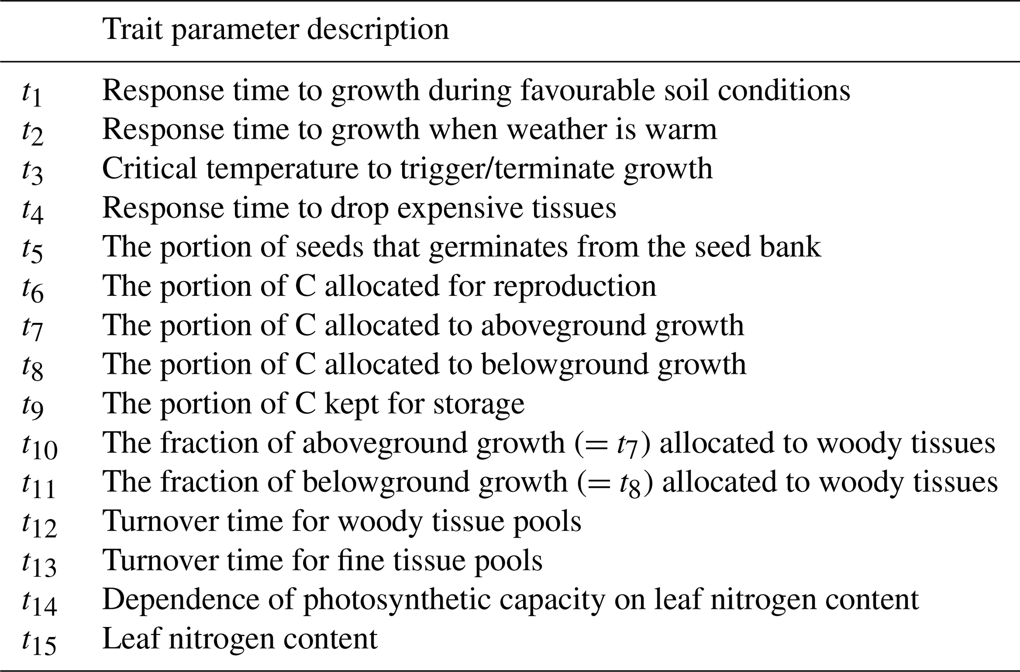
First, to mimic how plant growth responds to its environment, three aspects, determined by the four trait parameters t₁ to t₄, control the timing of growth: the length of the growing period, how fast a plant responds to environmental fluctuation, and when a plant starts shedding expensive tissues. A similar environment-dependent control is introduced for germination (trait parameters t₁ to t₃ and t₅). Second, to imitate life history strategies, a trade-off among growth, reproduction, and allocation to storage assuring survival is introduced. For this, allocation traits are key, namely the relative above- to below-ground growth and the relative allocation between woody and fine tissues (trait parameters t₅ to t₁₁). Last, a fast- or a slow-growth strategy is determined by the turnover time for woody and fine tissues (trait parameters t₁₂ and t₁₃). Related to this, a trade-off between a high assimilation rate (due to a high leaf nitrogen concentration) and the high respiratory costs for maintaining such high nitrogen concentrations is introduced (trait parameters t₁₄ and t₁₅). Note that technically, grasses are characterized by setting $t_{\mathrm{10}}=t_{\mathrm{11}}=\mathrm{0}$ so that there is no allocation to woody tissues.

2.1.2 Environmental filtering

The hypothesis of “Everything is everywhere, but the environment selects”, brought up by Becking (1934) (see De Wit and Bouvier, 2006; O'Malley, 2007), is widely used to link the biogeographic distribution of plants to environmental attributes. This “environmental filtering” hypothesizes that the environmental conditions will “naturally” select (filter out) a few surviving species from many – whichever species manages to survive the local environment can stay.

To illustrate this concept, imagine two types of trees with different allocation strategies: one invests more carbon in leaves than in roots; the other invests more in roots than in leaves. Imagine further that they grow in the same rainforest where it is warm year-round with plenty of rainfall. The tree with a more extensive canopy can grow faster than the tree with deep roots, as the former harvests more sunlight; because there is plenty of soil water available, having only shallow roots is sufficient to survive. However, if a long-lasting drought occurs, the high-canopy tree cannot survive beyond a certain aridity threshold while the deep-root tree might be able to persist because there might still be water available in deeper soil during drought stress. Hence, if the environment is such that despite high annual rainfall, precipitation varies strongly, the tree with shallow roots may not survive and may thus be filtered out.

To achieve environmental filtering, JeDi invokes a two-step approach:

•  

  Step 1 Trait generation: A large set of growth strategies is randomly generated from the 15-dimensional trait space, so all PGSs have different functional capabilities. For this number of randomly generated PGSs, we will use the term “potential diversity.”

•  

  Step 2 Environmental filtering: Initially, all strategies are allowed to grow everywhere over land, but only those that are able to maintain themselves in the given environment based on their inherent functional capabilities defined by the values of the trait parameters survive during the ongoing simulation. For this number of surviving PGSs we will use the term “actual diversity.”

Last, the modeling concept of JeDi can be briefly summarized as follows. All plant growth strategies have the same set of functional trade-off relationships and thus the same functional “ability.” Depending on the values of its plant trait parameters, each strategy has a specific functional “capability.” By sampling the 15-dimensional trait space randomly, JeDi creates a spectrum of plant growth strategies (potential diversity). Via environmental filtering, only a subset of PGSs survives (actual diversity). In comparison to the modelling of functional diversity by PFTs, JeDi thereby obtains a richer set of plant trait variation with more ecophysiological realism and less constraints on diversity.

2.1.3 Generation of random trait values

JeDi creates a spectrum of PGSs via random sampling in the 15-dimensional trait space spanned by the trait parameter values listed in Table B3. It is indeed challenging to explore such a high-dimensional space sufficiently to obtain a representative set of PGSs. For instance, already more than 32 000 combinations are needed to simulate all possible strategies if only two values are sampled for each dimension. This amount of strategies is not feasible due to limitations in computational resources. To nevertheless explore the multi-dimensional space even with a low number of strategies, the Latin-hypercube sampling (LHS) method is used (Stein, 1987) that assures a uniform sampling despite low coverage.

To apply LHS we let the values t₁ to t₁₅ range between 0 and 1. We first sample a chosen number of PGSs (typically up to a few thousand) in the 15-dimensional space by LHS. For some trait parameters, it is sufficient to have values between 0 and 1 (e.g., for t₅ representing a fraction), but for others, e.g., representing a temperature or time scale, they need later on to be converted to a physically meaningful range; these conversions are listed below as part of the model equations.

As mentioned above, we distinguish between grass-like and tree-like strategies in JeDi-BACH, where grasses are strategies without woody tissues. For grass-like strategies, the trait parameters that determine the growth of woody tissue must be zero. So, to obtain grass PGSs, we do the same random sampling as for woody PGSs but set $t_{\mathrm{10}}=t_{\mathrm{11}}=\mathrm{0}$. The proportion between the number of grass and tree PGSs must be chosen manually. For the simulations presented below, we choose 40 % of the total PGSs to be grass-like but the larger fraction of 60 % for tree-like PGSs because they need to survive much more specific combinations of parameter values than grasses.

2.1.4 Aggregation to ecosystem-scale

Like other DGVMs, the JeDi implementations also employ a mesh of grid cells to simulate the behaviour of vegetation in different geographical regions. Specific to JeDi-BACH is that the interaction between vegetation and the atmosphere is fully simulated. These interactions happen at the level of whole grid cells, i.e. the atmosphere doesn't “see” the contribution of the individual PGSs in a grid cell to albedo, roughness, and the various exchange fluxes, but only their combined contributions. This interaction may thus be conceived as happening at the ecosystem level, which is insofar realistic, as the interaction between the free atmosphere and the land surface is mediated by the boundary layer, where air parcels with different thermodynamic properties get heavily mixed. Nevertheless, some PGSs perform better than others under the ruling environmental conditions, their contributions should contribute more to the interaction.

To estimate the contribution of an individual strategy, “biomass-ratio theory” (Grime, 1998) is employed to aggregate terrestrial fluxes and functional properties to values at ecosystem level, as introduced in the context of JeDi by Pavlick et al. (2013). In the review of Grime (1998), experimental evidence is summarized that the dominant species are usually taller, more expansive in morphology, and have larger biomass. These large-extent dominant species thereby make a large total contribution to ecosystem properties like productivity. Based on this evidence, Grime hypothesized that the relative importance of individual species to the community is closely proportional to the relative contribution of that species to the total plant biomass of the community. Other studies support this theory as a reasonable approximation for measuring functional diversity in a plant community (Laliberté and Legendre, 2010; Díaz and Cabido, 2001). Thus, JeDi scales the contribution of a strategy to a grid-cell wide quantity by its relative contribution to the total biomass in the gridcell (compare Eq. 49).

It is worth noting that biomass scaling serves in particular as a broadly realistic measure of the competition between tree- and grass-type species that is otherwise not represented in JeDi. Trees benefit from their high canopy to intercept light at a higher level in a natural environment than grasses so that trees win the competition for light. Trees also have higher resistance to wildfires due to their woody structure. Because of the typically higher biomass of trees, biomass scaling thereby gives trees potentially more weight compared to grasses and thus reflects these competitional advantages of trees. Nevertheless, trees do not always have an advantage over grasses. In the early stage of succession, trees have a disadvantage over grasses because trees grow slowly and need to spend considerable energy on constructing and maintaining woody tissues. Hence, grasses can under certain conditions outcompete trees even though grass biomass is smaller. Therefore the structural advantage of trees to grow woody tissues may be over-estimated by biomass ratio theory. For instance, savanna ecosystems are known to be shaped by fire disturbances that affect woody vegetation differently than grasses. Currently, JeDi-BACH does not take over the fire disturbance scheme from JSBACH. Therefore, biomass ratio theory may predict an overly large share of tree biomass in these regions.

2.2 Six plant functional organs and their carbon dynamics

The dynamics of the six organs of the universal plant is modeled by the changes in their biomass content. Accordingly, each tree PGS has its own six carbon pools for storage, seed, leaves, stem, coarse root, and fine root, while a grass PGSs has two less (the two woody pools stem and coarse root are missing). Figure 1 illustrates the carbon pool structure of a tree-like strategy. The dynamics of plant growth and resource distribution among the six pools define the functional capabilities of a PGS. A PGS is alive as long as it maintains a positive carbon storage. When a strategy has a negative carbon balance, it eventually goes extinct as it runs out of storage carbon which it needs to keep functioning. The dynamics of the six pools is described in Eqs. (1)–(6) where the biomass of a specific organ is denoted by C_organ. As a whole they describe the growth of a PGS. Numerically the equations are solved at a daily time step by an Euler discretization. Details of the different terms appearing in these equations are described in subsequent sections.

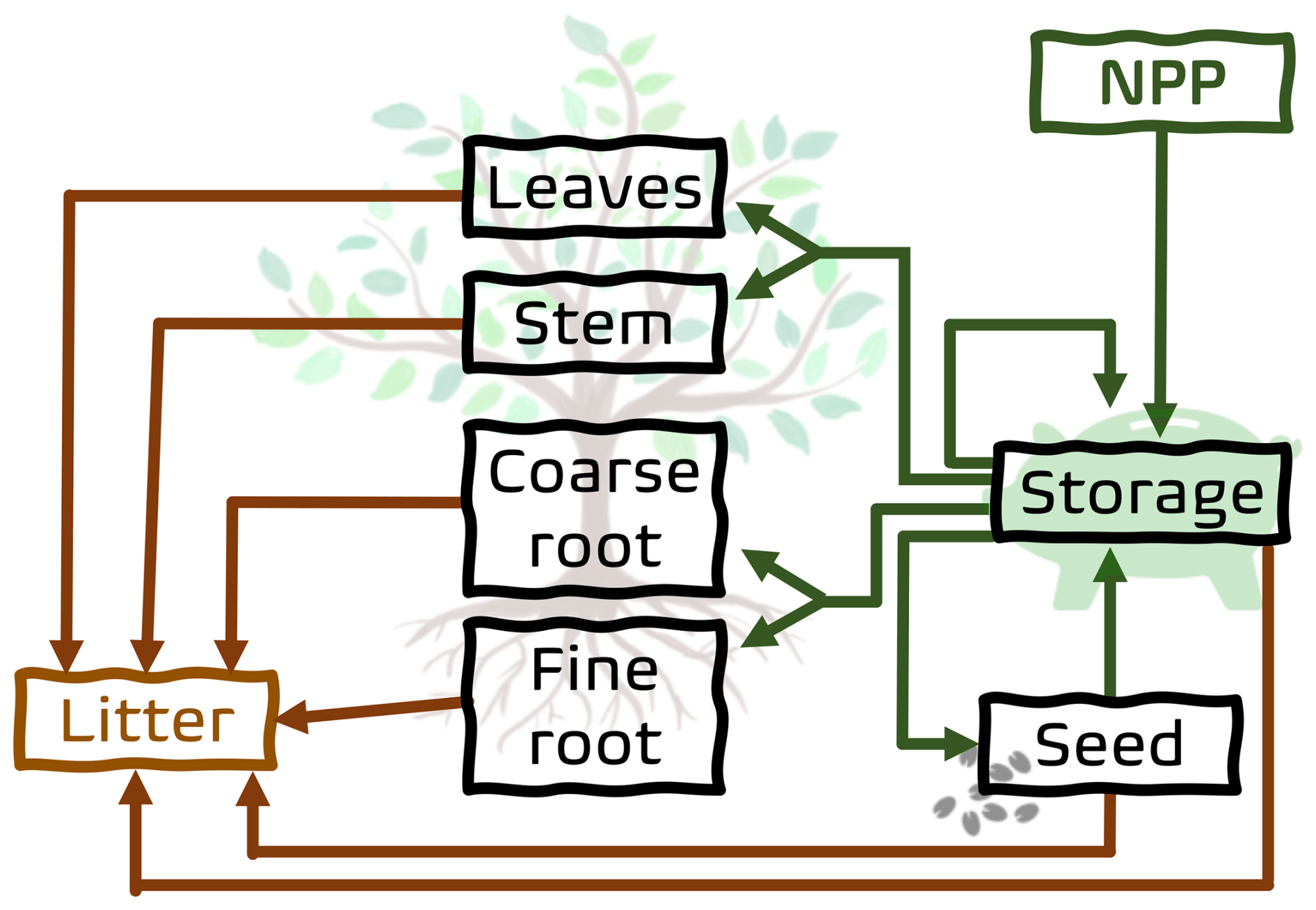
Figure 1 Structure of the carbon pool model of JeDi-BACH. Arrows indicate the carbon fluxes between the pools.

A plant grows by allocation of carbon gained through photosynthesis. JeDi has a separate storage pool to collect these photosynthesized sugars before they are distributed to grow other plant organs (compare Fig. 1). The dynamics of this pool is described by

$$\begin{array}{}\text{(1)}& \begin{array}{rl}{\displaystyle \frac{\mathrm{d}{\mathrm{C}}_{\mathrm{storage}}}{\mathrm{d}t}}& =\text{GPP}-R_{\text{m}}-{\mathrm{C}}_{\mathrm{storage}}\sum _{\begin{array}{c}\text{organ}\\ \ne \text{storage}\end{array}}{A}_{\text{organ}}\\ & -{\displaystyle \frac{{\mathrm{C}}_{\mathrm{storage}}}{{\mathit{\tau }}_{\text{storage}}}}+\text{GERM}.\end{array}\end{array}$$

Here the influx of photosynthesized sugars, called gross primary productivity (GPP), shows up as the first right-hand side term. Most of GPP is spent on maintaining existing tissues. This loss flux, called maintenance respiration R_m, is subtracted from GPP in Eq. (1). The difference NPP = GPP−R_m is called net primary production and can conceptually be considered as the net influx to the carbon model driving its dynamics (see Fig. 1). The next right-hand side term represents the loss of sugars to the other plant organs needed for their growth. The fraction of storage carbon distributed to the different organs is determined by the “allocation fractions” A_organ appearing under the sum over the organs. These allocation fractions determine the relative growth of the organs (“allometry”) and thus may be very different for different growth strategies. Accordingly, their values are directly obtained from the randomly chosen parameter values (see next section). The fourth right-hand side term describes the aging of storage cells by assuming that they die at a rate determined by a mean lifetime τ_storage.

The last right-hand side term GERM that adds to the storage pool in Eq. (1) is related to the germination of seeds. Their carbon dynamics is described by

$$\begin{array}{}\text{(2)}& {\displaystyle \frac{\mathrm{d}{\mathrm{C}}_{\mathrm{seed}}}{\mathrm{d}t}}={\mathrm{C}}_{\mathrm{storage}}{A}_{\text{seed}}(\mathrm{1}-k_{\text{RES}})-{\displaystyle \frac{{\mathrm{C}}_{\mathrm{seed}}}{{\mathit{\tau }}_{\text{seed}}}}-\text{GERM}.\end{array}$$

The GERM flux is subtracted here because the seeds must pay the carbon costs for sprouting of new plants.

The other two right-hand side terms in Eq. (2) are structurally identical to the two right-hand side terms in the dynamic equations for the pools of all the other plant organs:

$$\begin{array}{}\text{(3)}& {\displaystyle \frac{\mathrm{d}{\mathrm{C}}_{\mathrm{leaves}}}{\mathrm{d}t}}={\mathrm{C}}_{\mathrm{storage}}{A}_{\text{leaves}}(\mathrm{1}-k_{\text{RES,leaves}})-{\displaystyle \frac{{\mathrm{C}}_{\mathrm{leaves}}}{{\mathit{\tau }}_{\text{leaves}}}},\text{(4)}& {\displaystyle \frac{\mathrm{d}{\mathrm{C}}_{\mathrm{stem}}}{\mathrm{d}t}}={\mathrm{C}}_{\mathrm{storage}}{A}_{\text{stem}}(\mathrm{1}-k_{\text{RES,stem}})-{\displaystyle \frac{{\mathrm{C}}_{\mathrm{stem}}}{{\mathit{\tau }}_{\text{stem}}}},\text{(5)}& {\displaystyle \frac{\mathrm{d}{\mathrm{C}}_{\mathrm{csroot}}}{\mathrm{d}t}}={\mathrm{C}}_{\mathrm{storage}}{A}_{\text{csroot}}(\mathrm{1}-k_{\text{RES,csroot}})-{\displaystyle \frac{{\mathrm{C}}_{\mathrm{csroot}}}{{\mathit{\tau }}_{\text{csroot}}}},\text{(6)}& {\displaystyle \frac{\mathrm{d}{\mathrm{C}}_{\mathrm{fnroot}}}{\mathrm{d}t}}={\mathrm{C}}_{\mathrm{storage}}{A}_{\text{fnroot}}(\mathrm{1}-k_{\text{RES,fnroot}})-{\displaystyle \frac{{\mathrm{C}}_{\mathrm{fnroot}}}{{\mathit{\tau }}_{\text{fnroot}}}}.\end{array}$$

For growth all these organ pools receive carbon from the storage pool, but not the full amount C_storageA_organ that is deducted from the storage pool, but this amount is reduced by the construction costs C_storageA_organk_RES,organ needed for the buildup of cells (“growth respiration”); the values k_RES,organ determining the fraction of the available carbon needed for construction are fixed parameters. The terms $C/\mathit{\tau }$ describe a constant natural mortality by aging, but in the case of leaves and fine roots also senescence by shortening the turnover time during periods unsuitable for growth (see below).

2.3 Carbon allometry

The allometry of a plant, i.e. the relative size of its organs, depends in particular on how carbon resources are distributed between them. As resources are limited, the growth of each plant organ relative to the whole plant is thus critical for determining their fitness and survival. Concerning carbon, this distribution is determined in JeDi-BACH by the allocation fractions A_organ (compare Eqs. 1–6), which are obtained from the random trait parameter values t₆–t₁₁ (see Table B3) for the various organs by

$$\begin{array}{}\text{(7)}& \begin{array}{rl}& A_{\text{seed}}=F_{\text{grow}}{F}_{\text{seed}}{\displaystyle \frac{t_{\mathrm{6}}}{t_{\text{total}},}}\\ & A_{\text{stem}}=F_{\text{grow}}{\displaystyle \frac{t_{\mathrm{7}}}{t_{\text{total}}}}\cdot t_{\mathrm{10}},\\ & A_{\text{leaves}}=F_{\text{grow}}{\displaystyle \frac{t_{\mathrm{7}}}{t_{\text{total}}}}\cdot \left(\mathrm{1}-t_{\mathrm{10}}\right),\\ & A_{\text{csroot}}=F_{\text{grow}}{\displaystyle \frac{t_{\mathrm{8}}}{t_{\text{total}}}}\cdot t_{\mathrm{11}},\\ & A_{\text{fnroot}}=F_{\text{grow}}{\displaystyle \frac{t_{\mathrm{8}}}{t_{\text{total}}}}\cdot \left(\mathrm{1}-t_{\mathrm{11}}\right),\end{array}\end{array}$$

where

$$\begin{array}{}\text{(8)}& t_{\text{total}}:=t_{\mathrm{6}}+t_{\mathrm{7}}+t_{\mathrm{8}}+t_{\mathrm{9}}.\end{array}$$

Here F_grow and F_seed are “on-off” functions having values of either zero or one that determine the timing of plant growth and reproduction (see Eqs. 14 and 15 below).

By these equations, the amount of carbon distributed from the storage pool to the other organs is calculated in two steps (compare also Fig. 1). First, controlled by the trait parameters t₆–t₉, the carbon available for growth is split into fractions for seed ($t_{\mathrm{6}}/t_{\text{total}}$), the groups of above- and below-ground organs ($t_{\mathrm{7}}/t_{\text{total}}$, $t_{\mathrm{8}}/t_{\text{total}}$), and for the carbon remaining in the storage pool ($t_{\mathrm{9}}/t_{\text{total}}$), where t_total, defined in Eq. (8), denotes the sum of these four parameters so that

$$\begin{array}{}\text{(9)}& \sum _{i=\mathrm{6}}^{\mathrm{9}}{\displaystyle \frac{t_i}{t_{\text{total}}}}=\mathrm{1};\end{array}$$

this guaranties that not more carbon than available is distributed. Note that t₉ appears only in the definition (Eq. 8) of t_total and therefore determines the fraction of carbon that is not available for growth remains in the storage pool. In a second step, controlled by the trait parameter t₁₀ and t₁₁, the carbon available for above- and below-ground growth is further distributed to woody and non-woody organs. For example, t₁₀ determines the fraction of the available above-ground carbon put into the leaves organ (non-woody) while the rest 1−t₁₀ is put into the above-ground stem organ (woody). In addition, t₁₀ and t₁₁ determine whether a plant has a tree-like or a grass-like strategy by setting $t_{\mathrm{10}}=t_{\mathrm{11}}=\mathrm{0}$ for grasses. Last, this transfer of carbon from the storage pool to the organs is suppressed outside the growth period because during this time F_grow=0 (see Sect. 2.4.2).

2.4 Phenology

It is known from observations that the phenology, i.e. the seasonal timing of several key plant biological events, is tightly linked to the surrounding environment, such as the local climatic conditions and water availability (Lieth, 1974). For instance, leaf buds develop during spring when the weather gets warmer. During autumn, deciduous trees shed their leaves to reduce the loss of energy otherwise needed to maintain non-productive tissues during winter. The timing of these events varies substantially across different vegetation types and climate regions. As an example, consider the timing of the growth period. This is related to a trade-off: an early start of growth gives early access to resources but puts species at risk because weather is not always stably favorable to growth in early spring. Later during the year the environment becomes more stable so that for a later start of growth, the risk for a plant to fail is reduced. However, a late start comes with the disadvantage of a shorter growth period and less opportunity to assimilate carbon. Hence, depending on the ruling environment, different species may have developed different strategies to survive concerning phenology.

The phenological events considered in JeDi-BACH are the timing for the start and end of the growth period, the date of seed germination, and the on- and offset of senescence. These events are related to two environmental variables: the near-surface temperature and the relative soil moisture. During the year, phenological events happen typically only once or twice. But those environmental variables may fluctuate heavily from day to day so that these events cannot be triggered directly by them but by some time-mean behaviour. This is e.g. well known for many temperate species (Murray et al., 1989), where the budburst date is related to a temperature sum over the previous weeks. In JeDi-BACH we therefore determine phenological events from low pass filtered variables. Hence, before we describe the calculation of the various phenological events, we first introduce this concept of pseudo variables.

2.4.1 Pseudo variables

To determine the timing of phenological events, we use in JeDi-BACH the environmental variables that trigger them not directly but their low-pass filtered values, which we call “pseudo variables”. This technique, adapted from Reick et al. (2021), is similar to the method used by Pavlick et al. (2013) in JeDi-DGVM, but makes the low-pass filtering independent of the model time step.

The pseudo variable ${\stackrel{\mathrm{‾}}{X}}^n$ at time n is defined by

$$\begin{array}{}\text{(10)}& {\stackrel{\mathrm{‾}}{X}}^n={\displaystyle \frac{\mathrm{1}}{\mathcal{N}}}\sum _{n^{\prime }=-\mathrm{\infty }}^n{X}^n{e}^{-\left(n-n^{\prime }\right)\frac{\mathrm{\Delta }t}{\mathit{\tau }}},\mathcal{N}:=\sum _{n^{\prime }=-\mathrm{\infty }}^n{e}^{-\left(n-n^{\prime }\right)\frac{\mathrm{\Delta }t}{\mathit{\tau }}},\end{array}$$

where Xⁿ is the original environmental variable at time n that one aims to smoothe, τ characterizes the time length of memory of the low pass filter, and Δt is the length of the time step in the original data, typically the time step of the atmospheric model to which JeDi-BACH is coupled. The so defined pseudo variable stores the time-filtered behavior of the corresponding state variable by performing the averaging such that in each time step the most recent past is given the biggest weight, while the older the information, the less it is taken into account. The normalization 𝒩 is chosen such that the long time mean of the pseudo variable ${\stackrel{\mathrm{‾}}{X}}^n$ is equal to the long time mean of the original variable Xⁿ.

It can be shown that the recursion (Eq. 10) is solved by

$$\begin{array}{}\text{(11)}& {\stackrel{\mathrm{‾}}{X}}^{n+\mathrm{1}}={\displaystyle \frac{X^n}{\mathcal{N}}}+{\stackrel{\mathrm{‾}}{X}}^n{e}^{-\frac{\mathrm{\Delta }t}{\mathit{\tau }}},\mathcal{N}={\displaystyle \frac{\mathrm{1}}{\mathrm{1}-e^{-\frac{\mathrm{\Delta }t}{\mathit{\tau }}}}}.\end{array}$$

This is how ${\stackrel{\mathrm{‾}}{X}}^n$ is actually calculated in JeDi-BACH (the formula used in Pavlick et al., 2013, Eq. A.10, is obtained by setting $\mathit{\tau }=\mathcal{N}-\mathrm{1}$).

The so calculated pseudo variable ${\stackrel{\mathrm{‾}}{X}}^n$ mimics how plants store past environmental information. Accordingly, a PGS with a small value of τ (meaning a short memory) characterizes a responsive species that stores only recent environmental information. It reacts quickly once the environment is favorable. Likewise, a large value of τ (meaning a long memory) characterizes a conservative species that stores information about the recent past for a long time: this strategy responds slowly to changes in the environment.

2.4.2 Timing of plant growth

Carbon allocation happens only during the growth period. This is modelled by means of the on/off variable F_grow that allows or stops allocation (compare Eq. 7). The present section describes how F_grow is calculated.

In JeDi-BACH, the timing of plant growth depends on ambient temperature and the relative soil wetness. Three pseudo environmental variables are used to determine the timing (compare Eq. 11):

$$\begin{array}{}\text{(12)}& \begin{array}{rl}{\displaystyle }{\stackrel{\mathrm{‾}}{W}}_{\text{grow}}^{n+\mathrm{1}}& {\displaystyle }=W^n\left(\mathrm{1}-e^{-\frac{\mathrm{\Delta }t}{{\mathit{\tau }}_W}}\right)+{\stackrel{\mathrm{‾}}{W}}_{\text{grow}}^n\cdot e^{-\frac{\mathrm{\Delta }t}{{\mathit{\tau }}_W}},{\mathit{\tau }}_W={\mathrm{10}}^{\mathrm{1.1}{t}_{\mathrm{1}}+\mathrm{0.9}}\text{d},\\ {\displaystyle }{\stackrel{\mathrm{‾}}{T}}_{\text{grow}}^{n+\mathrm{1}}& {\displaystyle }=T^n\left(\mathrm{1}-e^{-\frac{\mathrm{\Delta }t}{{\mathit{\tau }}_T}}\right)+{\stackrel{\mathrm{‾}}{T}}_{\text{grow}}^n\cdot e^{-\frac{\mathrm{\Delta }t}{{\mathit{\tau }}_T}},{\mathit{\tau }}_T={\mathrm{10}}^{\mathrm{1.1}{t}_{\mathrm{2}}+\mathrm{0.9}}\text{d},\\ {\displaystyle }{\stackrel{\mathrm{‾}}{\mathrm{\Delta }T}}_{\mathrm{30}\text{d}}^{n+\mathrm{1}}& {\displaystyle }=\mathrm{\Delta }{T}^n\left(\mathrm{1}-e^{-\frac{\mathrm{\Delta }t}{{\mathit{\tau }}_T}}\right)+{\stackrel{\mathrm{‾}}{\mathrm{\Delta }T}}_{\mathrm{30}\mathrm{d}}^n\cdot e^{-\frac{\mathrm{\Delta }t}{\mathit{\tau }}},\mathit{\tau }=\mathrm{30}\text{d}.\end{array}\end{array}$$

Here Wⁿ is the relative soil moisture within the root zone at time step n, Tⁿ is the near-surface air temperature at that time step, and $\mathrm{\Delta }{T}^n=T^n-T^{n-\mathrm{1}}$ is the stepwise difference in temperatures. ${\stackrel{\mathrm{‾}}{W}}_{\text{grow}}^n$, ${\stackrel{\mathrm{‾}}{T}}_{\text{grow}}^n$, and ${\stackrel{\mathrm{‾}}{\mathrm{\Delta }T}}_{\mathrm{30}\mathrm{d}}^n$ are the pseudo soil wetness, pseudo surface air temperature, and pseudo daily temperature change, averaged over periods τ_W, τ_T, and τ. While equivalents of ${\stackrel{\mathrm{‾}}{W}}_{\text{grow}}^n$ and ${\stackrel{\mathrm{‾}}{T}}_{\text{grow}}^n$ also exist in other JeDi implementations, ${\stackrel{\mathrm{‾}}{\mathrm{\Delta }T}}_{\mathrm{30}\mathrm{d}}$ is newly introduced in JeDi-BACH to improve the timing of the end of the growth period particularly in mid-to high-latitude ecoregions (see further remarks in Appendix C1). Note that the memory times τ_W and τ_T are different for different PGSs – they are determined by the randomly chosen trait parameters values t₁ and t₂ –, while τ is a global model parameter. The way τ_W and τ_T are calculated from t₁ and t₂ (see Eq. 11) assures that the memory times range between one week ($t_{\mathrm{1}}=t_{\mathrm{2}}=\mathrm{0}$) and a few months ($t_{\mathrm{1}}=t_{\mathrm{2}}=\mathrm{1}$).

The timing of growth depends in addition on the random trait variable t₃ that determines the temperatures for the potential start and end of the growth period, called T_start and T_end. These are obtained by scaling of t₃ to temperature ranges [$-\mathrm{5},\mathrm{15}$] ° C, and [10, 15] ° C by setting

$$\begin{array}{}\text{(13)}& \begin{array}{rl}{\displaystyle }{T}_{\text{start}}& {\displaystyle }=-\mathrm{5}+\mathrm{20}{t}_{\mathrm{3}},\\ {\displaystyle }{T}_{\text{end}}& {\displaystyle }=\mathrm{10}+\mathrm{5}{t}_{\mathrm{3}}.\end{array}\end{array}$$

Next one introduces the auxiliary on/off switch F_T by:

$$\begin{array}{}\text{(14)}& F_T=\left\{\begin{array}{ll}\mathrm{1}& \text{if}{\stackrel{\mathrm{‾}}{T}}_{\text{grow}}>T_{\text{start}}\text{and}{\stackrel{\mathrm{‾}}{\mathrm{\Delta }T}}_{\mathrm{30}\mathrm{d}}\ge \mathrm{0}\\ \mathrm{0}& \text{if}{\stackrel{\mathrm{‾}}{T}}_{\text{grow}}<T_{\text{end}}\text{and}{\stackrel{\mathrm{‾}}{\mathrm{\Delta }T}}_{\mathrm{30}\mathrm{d}}<\mathrm{0}\\ \text{unchanged}& \text{otherwise }\end{array}\right..\end{array}$$

This switch encodes not only whether the environment is within a strategy's thermal adaptation range defined by T_start and T_end, but by considering the sign of ${\stackrel{\mathrm{‾}}{\mathrm{\Delta }T}}_{\mathrm{30}\mathrm{d}}$ also whether the environment is warming or cooling. Finally, combing F_T with the ruling soil moisture conditions encoded in ${\stackrel{\mathrm{‾}}{W}}_{\text{grow}}$, the switch F_grow controlling growth is given by

$$\begin{array}{}\text{(15)}& F_{\text{grow}}=\left\{\begin{array}{ll}\mathrm{1}& \text{if}{\stackrel{\mathrm{‾}}{W}}_{\text{grow}}\ge \mathit{\alpha }\text{and}{F}_T=\mathrm{1}\\ \mathrm{0}& \text{otherwise},\end{array}\right..\end{array}$$

where α is the threshold (α=0.4) for soil wetness that determines the potential start of the growth period. Thereby the growth period starts (F_grow=1) when the relative soil wetness ${\stackrel{\mathrm{‾}}{W}}_{\text{grow}}$ is greater than 0.4 and the ambient temperature is favourable, otherwise the growth period ends (F_grow=0).

2.4.3 Timing of germination and seed production

The dynamics of the seed pool C_seed (see Eq. 2) are determined by two time-dependent fluxes, the carbon input from the production of seedlings (first right hand side term) and the carbon loss by germination GERM.

In JeDi it is assumed that seed production happens only during the growth period and if in addition the daily carbon balance is positive. This behaviour is encoded in Eq. (7) for the allocation fraction A_seed, which controls the input term in Eq. (2): A_seed is non-zero only when F_grow=1 and if in addition F_seed is non-zero. F_seed is the on-off switch defined by

$$\begin{array}{}\text{(16)}& F_{\text{seed}}=\left\{\begin{array}{ll}\mathrm{1}& \text{if NPP}>\mathrm{0}\\ \mathrm{0}& \text{otherwise},\end{array}\right.\end{array}$$

so that seeds are only produced at days with positive net primary productivity (NPP).

For the loss flux GERM it is assumed that germination of seedlings happens only when both temperature and topsoil moisture are favorable. This behaviour is encoded in the on-off switch F_germ, defined as follows. Let ${\stackrel{\mathrm{‾}}{W}}_{\mathrm{5}\text{cm}}$ denote the relative soil moisture in the top 5 cm of the soil. Then

$$\begin{array}{}\text{(17)}& {\stackrel{\mathrm{‾}}{W}}_{\mathrm{5}\text{cm}}^{n+\mathrm{1}}=W_{\mathrm{5}\text{cm}}\left(\mathrm{1}-e^{-\frac{\mathrm{\Delta }t}{{\mathit{\tau }}_W}}\right)+{\stackrel{\mathrm{‾}}{W_{\mathrm{5}\text{cm}}}}^n\cdot e^{-\frac{\mathrm{\Delta }t}{{\mathit{\tau }}_W}}\end{array}$$

is the corresponding pseudo variable, where τ_W is the characteristic memory time for pseudo soil moisture (compare τ_W in Eq. (12). The switch for germination is then defined by

$$\begin{array}{}\text{(18)}& F_{\text{germ}}=\left\{\begin{array}{ll}\mathrm{1}& \text{if}{\stackrel{\mathrm{‾}}{W}}_{\mathrm{5}\text{cm}}\ge \mathrm{0.5}\text{and}{F}_T=\mathrm{1}\\ \mathrm{0}& \text{otherwise}.\end{array}\right.\end{array}$$

This switch gives 1 when the top 5 cm of the soil are filled more than half, and if in addition temperatures are favorable for growth, as expressed by the temperature switch F_T=1 (compare Eq. 14). With this germination switch, the germination flux appearing in the seed equation (Eq. 2) is set to

$$\begin{array}{}\text{(19)}& \text{GERM}=F_{\text{germ}}{\mathit{\gamma }}_{\text{germ}}{\mathrm{C}}_{\mathrm{seed}},{\mathit{\gamma }}_{\text{germ}}={\mathrm{10}}^{\mathrm{3}{t}_{\mathrm{5}}-\mathrm{3}},\end{array}$$

so that when germination happens (F_germ=1), the amount of carbon invested into germination is determined by the available seed carbon C_seed and the “germination fraction” γ_germ. Its value is constructed from the random trait parameter value t₅ such that it ranges between 10⁻³ to 1. A small value of γ_germ defines a conservative PGS that germinates only a small amount of its seeds; a large value of γ_germ characterizes a PGS which invests heavily into reproduction.

2.4.4 Senescence and turnover

Plant productivity is considerably reduced outside the growth period and during periods of harsh environmental conditions. For instance, plants quickly deplete their storage carbon (e.g., starch or sugars) during persisting droughts or extreme cold events when maintenance costs are higher than photosynthetic production. Once production is constrained over a prolonged period, such negative carbon flow can eventually lead to the death of a plant. To survive these harsh periods, plants abandon some of their fine tissues to reduce maintenance costs. This shedding of fine tissues due to senescence is modelled in JeDi-BACH by enhancing the respective turnover times for leaves τ_leaves and for fine roots τ_fnroots in the carbon equations (Eqs. 3 and 6) beyond their background value reflecting permanent aging. Their permanent natural aging rate $\mathrm{1}/{\mathit{\tau }}_{\mathrm{leaves},\mathrm{0}}$ is calculated from the random trait parameter value t₁₃ by setting leaf longevity τ_leaves,0 to

$$\begin{array}{}\text{(20)}& {\mathit{\tau }}_{\mathrm{leaves},\mathrm{0}}={\displaystyle \frac{\mathrm{365}}{\mathrm{12}}}{\mathrm{10}}^{\mathrm{2}{t}_{\mathrm{13}}}\text{d}\end{array}$$

so that it ranges between 1 and 100 months. Once a PGS experiences environmental conditions unsuitable for growth the turnover rates $\mathrm{1}/{\mathit{\tau }}_{\text{leaves}}$ and $\mathrm{1}/{\mathit{\tau }}_{\text{fnroot}}$ of leaves and fine-roots are enhanced by adding to the permanent background rate the globally prescribed senescence rate $\mathrm{1}/{\mathit{\kappa }}_{\text{SEN}}$:

$$\begin{array}{}\text{(21)}& {\mathit{\tau }}_{\text{fnroot}}={\mathit{\tau }}_{\text{leaves}}={\left({\displaystyle \frac{\mathrm{1}}{{\mathit{\tau }}_{\mathrm{leaves},\mathrm{0}}}}+F_{\text{stress}}\cdot {\displaystyle \frac{\mathrm{1}}{{\mathit{\kappa }}_{\text{SEN}}}}\right)}^{-\mathrm{1}}.\end{array}$$

Here F_stress is an “on-off” switch indicating good/bad environmental conditions that are detected by checking the sign of net primary productivity NPP and of the associated pseudo variable $\stackrel{\mathrm{‾}}{\text{NPP}}$:

$$\begin{array}{}\text{(22)}& F_{\text{stress}}=\left\{\begin{array}{ll}\mathrm{1}& \text{if}\stackrel{\mathrm{‾}}{\text{NPP}}<\mathrm{0}\text{and NPP}<\mathrm{0}\\ \mathrm{0}& \text{otherwise},\end{array}\right.\end{array}$$

where

$$\begin{array}{}\text{(23)}& {\displaystyle }{\stackrel{\mathrm{‾}}{\text{NPP}}}^{n+\mathrm{1}}& {\displaystyle }={\text{NPP}}^n\left(\mathrm{1}-e^{-\frac{\mathrm{\Delta }t}{{\mathit{\tau }}_{\text{NPP}}}}\right)+{\stackrel{\mathrm{‾}}{\text{NPP}}}^n\cdot e^{-\frac{\mathrm{\Delta }t}{{\mathit{\tau }}_{\text{NPP}}}},\text{(24)}& {\displaystyle }{\mathit{\tau }}_{\text{NPP}}& {\displaystyle }={\mathrm{10}}^{\mathrm{1.1}{t}_{\mathrm{4}}+\mathrm{0.9}}\text{d}.\end{array}$$

Here τ_NPP is the characteristic memory time of $\stackrel{\mathrm{‾}}{\text{NPP}}$ constructed from the random trait parameter value t₄ so that memory time ranges from weeks to months.

To briefly wrap up, senescence is enhanced when both $\stackrel{\mathrm{‾}}{\text{NPP}}$ and NPP are negative. Once triggered, the expensive tissues (leaves, fine roots) deteriorate substantially faster than at natural aging rate. In this way, plants increase their chance for survival by reducing their maintenance costs to avoid a persistent negative carbon balance.

Coming now to the turnover of the other tissues, the stems and coarse roots are given the same turnover time by setting (compare Eqs. 4 and 5)

$$\begin{array}{}\text{(25)}& {\mathit{\tau }}_{\text{stem}}={\mathit{\tau }}_{\text{csroot}}=\mathrm{365}\left(\mathrm{79}{t}_{\mathrm{12}}+\mathrm{1}\right)\text{d}.\end{array}$$

Note that these turnover times are obtained from the random trait parameter value t₁₂ such that they range from one to eighty years. While the turnover times of these woody tissues are determined by a random trait, the turnover times of the seed and storage organs are given fixed values, namely τ_seed=3 year and τ_storage=1 year (compare Table ).

2.5 Leaf properties: Photosynthesis, Nitrogen, and Lifespan

Leaves intercept sunlight for photosynthesis and assimilate carbon for growth. The amount of photosynthetic production depends on several leaf traits like leaf size, but also on the ambient environmental conditions such as light, moisture, and temperature. In the carbon balance equations, photosynthesis shows up as gross primary production, denoted as GPP (see Eq. 1). The present section explains how GPP is obtained in JeDi-BACH and which random traits are involved.

2.5.1 JSBACH Photosynthesis module and leaf area index

GPP is calculated in JeDi-BACH by employing the photosynthesis module of JSBACH. Only two variables are needed from JeDi to employ the JSBACH photosynthesis module in JeDi-BACH. One of them is a measure of plant water stress, whose calculation is explained in the separate Sect. 2.6 below. The other is the leaf area index LAI. This section explains how the LAI is calculated and how then GPP is obtained from the JSBACH photosynthesis module.

The JSBACH photosynthesis module consists of two parts: a canopy radiation model to calculate the radiation absorbed by the leaves for photosynthesis, and two photosynthesis models, that of Farquhar et al. (1980) for the C₃ photosynthetic pathway and that of Collatz et al. (1992) for the C₄ photosynthetic pathway. In practice, we use the C₃ photosynthesis module for all tree-type PGSs. For grass-type PGSs, a fraction of them is assigned to be handled by the C₃ module, while for the remaining grass-type PGSs we use the C₄ module. The specific C₃ $/$ C₄ fraction is prescribed during model initialization. In contrast to the empirical photosynthesis model used in the JeDi-DGVMs of Kleidon and Mooney (2000, Eq. 9) and Pavlick et al. (2013, Eq. A.15), the Farquhar and the Collatz models are explicit representations of the enzyme kinetics underlying photosynthetic productivity, depending in particular on ambient temperature, and for the C₃ model also on the ambient CO₂ concentration. Via the parameters for maximum carboxylation rate (Farquhar) and PEPCase specificity (Collatz) productivity depends in these models implicitly on the nitrogen content of leaves, that had to be made explicit to be consistent with JeDi (see Sect. 2.5.2 below). The canopy radiation model providing the radiation input to the photosynthesis models is based on a two-stream approximation of the radiation balance in the canopy (Sellers, 1987), in contrast to Lambert-Beer's law employed in the different JeDi-DGVMs (see Kleidon and Mooney, 2000, Eq. 8; Pavlick et al., 2013, Eq. A.16; Rius et al., 2023, Eqs. SM17, SM 18). Calculations are performed every time step taking as input from the atmosphere model the down-welling diffuse and direct radiation while accounting for the position of the sun at that time step. In JeDi-BACH, the tree-like strategies are assumed to perform C₃ photosynthesis, so for them, the Farquhar model is used, while for the grass-like strategies, the Collatz model for C₄ plants is employed. More details on the JSBACH photosynthesis module are found in Reick et al. (2021).

To obtain GPP for a particular PGS, JeDi-BACH needs to pass its LAI to the JSBACH photosynthesis module. The LAI of a canopy is defined as the one-sided leaf area per unit ground area. It is calculated from the leaf biomass C_leaves by

$$\begin{array}{}\text{(26)}& \text{LAI}=\text{SLA}\cdot {\mathrm{C}}_{\mathrm{leaves}},\end{array}$$

where SLA denotes the specific leaf area, defined as leaf area per mole leaf carbon. The SLA value is a PGS-specific parameter obtained in JeDi from the random trait parameter t₁₃: From the works of Wright et al. (2004) and Reich et al. (1997) on the leaf economic spectrum it is known that the SLA is closely related to leaf longevity τ_leaves,0 by

$$\begin{array}{}\text{(27)}& \text{SLA}=\mathrm{0.323}{\left({\displaystyle \frac{\mathrm{365}\text{d}}{{\mathit{\tau }}_{{\mathrm{leaves}}_{\mathrm{0}}}}}\right)}^{\mathrm{0.46}}{\displaystyle \frac{{\mathrm{m}}^{\mathrm{2}}\mathrm{leaf}}{\mathrm{mol}\mathrm{C}}},\end{array}$$

where the dependence of ${\mathit{\tau }}_{{\mathrm{leaves}}_{\mathrm{0}}}$ on t₁₃ was already introduced by Eq. (20) above. Using LAI together with the water stress factor α_stress (see Sect. 2.6) when calling the photosynthesis module of JSBACH, it returns the photosynthetic assimilation rate A_stressed in the presence of water stress. From this GPP is obtained by

$$\begin{array}{}\text{(28)}& \text{GPP}=\text{LAI}\cdot A_{\text{stressed}}.\end{array}$$

In order to obtain GPP in this way a slight modification of the calculations in the JSBACH photosynthesis module got necessary. While in reality the LAI is limited by plant hydraulics and mechanical stability to values up to typically 12 (Larcher, 1996, Table 2.18), such constraints are missing in the carbon allocation for leaves in JeDi. Therefore, as also known from other implementations of JeDi, some PGSs may develop an unrealistically large area index up to 30–50. The reason for such behaviour is that in JeDi, the allocation fractions to different organs, randomly chosen during initialization for each PGS, are static. Consequently, carbon investment into leaves continues even when, due to self-shading, further increases in LAI enhance productivity only marginally (which occurs from about LAI =6 onward). This can lead to some PGSs having unrealistically large LAI values due to their specific allocation parameters. Additionally, their carbon investment becomes uneconomic because the additional respiration costs (which grow linearly with allocated leaf carbon) are not compensated by increased productivity. To prevent growing such unproductive tissues in JeDi-BACH we introduced an additional parameter fapar_max that limits the “fraction of absorbed photosynthetically active radiation” (fapar) in the canopy to fapar_max=0.9. Thereby the photon flux passed from the canopy radiation calculations to the photosynthesis routines gets capped at 90 %, which limits productivity and thereby reduces the risk of uneconomic overinvestment into the growth of unproductive leaf tissues. Indeed, a better way to prevent unrealistically large LAI values would be to replace the linear JeDi allometry of Eq. (7) by a nonlinear model that limits carbon allocation to the various organs more realistically (see e.g. Niklas and Enquist, 2002). But this would be a severe structural change of JeDi, and since our main concern with this first version of JeDi-BACH is the interaction with climate, we decided for this simpler although less justified approach by introducing fapar_max.

2.5.2 Leaf traits and the photosynthesis-nitrogen relationship

Plants develop a competitive strategy to cope with limitations in different regions, and nitrogen is one of the mineral nutrients most limiting to plant growth (Vitousek and Howarth, 1991). The enzyme that synthesizes carbon in leaves (called Rubisco) is rich in nitrogen, which explains the observed strong relationship between nitrogen content and the photosynthetic capacity of a leaf (Field and Mooney, 1986; Reich et al., 1997, 1998, 2008). Leaves with higher nitrogen content (per leaf area) tend to have higher photosynthetic capacities and high stomatal conductance. This allows plants to gain carbon rapidly but at the cost of high rates of water loss and high maintenance costs. Conversely, plants with low photosynthetic capacities tend to have low stomatal conductance to conserve water. By a cross-continent analysis of various plant traits, Wright et al. (2004) found a trade-off between traits that maximize photosynthetic rate and traits that maximize leaf longevity. This relationship is denoted by the authors as the “leaf economics spectrum”. Leaf longevity is found to be correlated to leaf thickness. Leaves with a shorter lifespan tend to be thinner and are thus cheaper in terms of construction costs. Conversely, long-lived leaves are constructional expensive, so they are often thick, dense, and structurally more robust to withstand harsh environments (Reich et al., 1997; Wright et al., 2004). These observed correlations are used to construct leaf traits and trade-offs in JeDi-BACH.

Three leaf traits are used in JeDi-BACH: leaf longevity, specific leaf area, and leaf nitrogen content. How leaf longevity τ_leaves,0 is obtained from the random trait parameter t₁₄ and how SLA is obtained from τ_leaves,0 has already been specified in Eqs. (20) and (27). It remains to be explained how leaf nitrogen content appears as a trait in JeDi-BACH.

A key parameter of the Farquhar photosynthesis model implemented in JSBACH is the maximum assimilation rate $V_{\text{max}}^{\mathrm{25}}$ per leaf area at reference temperature 25° C which determines the availability of the RuBisCo enzyme in the Calvin cycle of C₃ photosynthesis. $V_{\text{max}}^{\mathrm{25}}$ correlates strongly with the nitrogen content of the leaves (Field and Mooney, 1986; Reich et al., 1997). To account for this dependence on leaf nitrogen content [N], we set, following Kattge et al. (2009, Eq. 1),

$$\begin{array}{}\text{(29)}& V_{\text{max}}^{\mathrm{25}}=i_v+s_v*\left[\mathrm{N}\right].\end{array}$$

Here i_v=4.19 mol C m⁻² leaf and $s_v=\mathrm{280}*t_{\mathrm{14}}+\mathrm{130.2}$ mol C mol N⁻¹ s⁻¹ are parameters that we obtained by a linear regression of the data from Table 2 in that study. To complete the calculation of $V_{\text{max}}^{\mathrm{25}}$ we determine the leaf nitrogen content from the random trait parameter t₁₅ by setting

$$\begin{array}{}\text{(30)}& \left[\mathrm{N}\right]=\mathrm{0.0457}+\mathrm{0.211}*t_{\mathrm{15}}{\text{mol\hspace{0.17em}N\hspace{0.17em}m}}^{-\mathrm{2}}\text{leaf}.\end{array}$$

The numbers in this formula were chosen such that thereby [N] covers the range of the more than 700 observational data from a broad range of C₃ species in Kattge et al. (2009). Besides $V_{\text{max}}^{\mathrm{25}}$ the other main parameter of the Farquhar photosynthesis model is the electron transport capacity J_max. As in JSBACH, also in JeDi-BACH one uses the (undocumented) approximate relation (compare Kattge and Knorr, 2007)

$$\begin{array}{}\text{(31)}& J_{\text{max}}=\mathrm{1.9}{V}_{\text{max}}^{\mathrm{25}},\end{array}$$

where the chosen factor 1.9 falls within the range of values found for broadleaved and coniferous trees in the literature (Kattge and Knorr, 2007; Wullschleger, 1993; Walker et al., 2014).

For the Collatz model of C₄ photosynthesis there is a similar key parameter, namely the PEPCase specificity (for simplicity also called $V_{\text{max}}^{\mathrm{25}}$ in JSBACH) that measures the availability of the PEPCase enzyme by which C₄ plants achieve the high intra-cell CO₂ concentrations making them so productive. Also, the PEPCase specificity should depend on the leaf nitrogen content (Collatz et al., 1992), but because of lack of data, in the current implementation of JeDi-BACH, this nitrogen nexus is ignored so that for the C₄-photosynthesis of grass-like strategies, all parameters are taken over from JSBACH.

2.6 Rooting strategies and water stress

As already noted in the previous section, to link JeDi with the photosynthesis module of JSBACH, one must provide besides the LAI also some measure of water stress. More precisely, the water stress status must be provided in the form of the water stress factor α_stress ranging from 0 (extreme water stress) to 1 (absence of water stress). Different to the other JeDi-models (Kleidon and Mooney, 2000; Pavlick et al., 2013; Rius et al., 2023), this section explains how the new calculation of α_stress works in JeDi-BACH.

Roots serve several critical functions related to the survival of plants. They anchor plants in the ground and, depending on the size of the roots, supply them with soil water and nutrients, both essential for photosynthesis and growth. Roots function like pipes connecting the water from the soil level with the atmosphere. Soil water diffuses into roots following the gradient of the hydraulic potential and moves through the xylem to the canopy. There, depending on the size of the leaves, the water is transpired to the atmosphere via stomata at the leaf surfaces. Besides the soil water accessible by roots, thus also the ambient atmospheric conditions affect plant productivity. When the ambient atmosphere is saturated, the water vapor gradient between the leaf surfaces and the surrounding air vanishes. This suppresses transpiration and plants react by opening their stomata wider to improve the access to atmospheric CO₂ without risk to loose additional water (e.g. Cunningham, 2004). But if these conditions last longer, the suppression of transpiration creates stress for the plants because they need the xylem water to keep flowing to thrive. In particular, with a slowing down of the water flux across the plants, the provision of nutrients deteriorates and the accumulation of photosynthesates from the ongoing photosynthesis may lead to its down regulation (Paul and Foyer, 2001), possibly explaining the down grading of photosynthesis at low vapor pressure deficit in Amazonia (Chen et al., 2022). Hence not only the sizes of roots and leaves, but the whole soil-plant-atmosphere continuum is of importance for the presence or absence of water stress. Accordingly, JeDi-BACH calculates the water stress factor α_stress jointly from the (relative) size of roots and leaves, the soil-water availability in the root zone, and the water vapour status of the ambient atmosphere. But before presenting how all these aspects are combined into a single expression for α_stress, first the close link between root size and soil water availability is discussed in the next subsection.

2.6.1 Pipe model and rooting depth

As seen from Eqs. (5) and (6), concerning carbon the root system is partitioned into two functional pools: the coarse roots C_csroot and the fine roots C_fnroot. Coarse roots are woody tissues that can penetrate deep into the soil, supporting the network of fine roots. Fine roots are hairy fine tissues that grow into tiny soil pores to suck up soil water. Fine-root tissues provide plant's with the actual ability to access soil water while the root depth, determined by the coarse roots, is the key factor determining the total amount of soil water accessible by the plants.

Inspired by the work of Shinozaki et al. (1964) (see also the recent review Lehnebach et al., 2018), the whole leaves-stems-coarse-roots-fine-roots system is treated as an assemblage of pipes connecting soil water with the atmosphere. The upper ends are the leaf stomata, while the lower ends are the fine roots. In between, stem and coarse roots form “pipes.” A schematic diagram of root pipes growing over a cross-section of soil is shown in Fig. 2 for illustration. Following the implementation of the original JeDi-DGVM (Kleidon and Mooney, 2000), the depths of the lower end, namely the root depth, is determined by the size of the coarse roots carbon pool C_csroot. The relation used is Eq. (37) below (compare Kleidon and Mooney, 2000, Eq. 8; Pavlick et al., 2013, Eq. A.11). Since so far no justification for this expression seems to be published, we present here a detailed derivation.

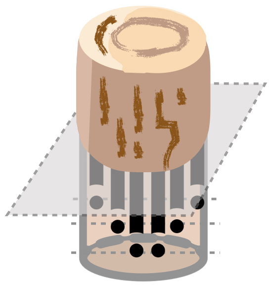
Figure 2 Sketch of the root pipes in a soil column. The black lines indicate the root pipes and the black dots indicate the pipe ends. By the assumption of a constant density of pipe ends, the number of pipes increases towards the surface.

Let a soil column of cross-sectional area A be interspersed with root pipes (the black lines in Fig. 2). JeDi assumes that water uptake by fine roots happens homogeneously throughout the soil column. In the pipe picture this amounts to assuming that the density of pipe ends ρ (“pipe ends” are shown as solid dots in Fig. 2) is constant within the soil column. Thereby, the density of root pipes increases towards a maximum at the surface. By these assumptions, the number of root pipes N_pipe at depth z is obtained by

$$\begin{array}{}\text{(32)}& N_{\text{pipe}}\left(z\right)=\underset{z}{\overset{l_{\text{r}}}{\int }}\mathit{\rho }A\mathrm{d}z=\mathit{\rho }A(l_{\mathrm{r}}-z),\end{array}$$

where l_r denotes the depth of the considered soil column that we interpret here as root depth. Assuming that all coarse-root carbon is used to construct pipes and letting c_spl denote the specific pipe length, i.e. the length of pipe grown per unit coarse-root carbon, the total length L_pipe of all pipes in the considered soil column built by the available coarse root carbon C_csroot is

$$\begin{array}{}\text{(33)}& L_{\text{pipe}}\left(l_{\text{r}}\right)=c_{\text{spl}}\cdot {\mathrm{C}}_{\mathrm{csroot}}\cdot A.\end{array}$$

On the other hand, the total length of root pipes in the soil column down to a depth d can as well be obtained from the vertical distribution of the above determined number of root pipes:

$$\begin{array}{}\text{(34)}& \begin{array}{rl}{L}_{\text{pipe}}\left(d\right)& =\underset{\mathrm{0}}{\overset{d}{\int }}{N}_{\text{pipe}}\left(z\right)\mathrm{d}z=\mathit{\rho }A\left(l_{\text{r}}z-{\displaystyle \frac{\mathrm{1}}{\mathrm{2}}}{z}^{\mathrm{2}}\right){|}_{\mathrm{0}}^d\\ & =\mathit{\rho }A\left(l_{\text{r}}d-{\displaystyle \frac{\mathrm{1}}{\mathrm{2}}}{d}^{\mathrm{2}}\right).\end{array}\end{array}$$

Equating these two equations for L(d) at root depth d=l_r gives

$$\begin{array}{}\text{(35)}& L_{\text{pipe}}\left(l_{\text{r}}\right)=\mathit{\rho }A\left(l_{\text{r}}^{\mathrm{2}}-{\displaystyle \frac{\mathrm{1}}{\mathrm{2}}}{l}_{\text{r}}^{\mathrm{2}}\right)={\displaystyle \frac{\mathrm{1}}{\mathrm{2}}}{l}_{\text{r}}^{\mathrm{2}}\mathit{\rho }A=c_{\text{spl}}{\mathrm{C}}_{\mathrm{csroot}}A.\end{array}$$

Solution for rooting depth l_r reveals

$$\begin{array}{}\text{(36)}& l_{\text{r}}=\sqrt{{\displaystyle \frac{\mathrm{2}{c}_{\text{spl}}{\mathrm{C}}_{\mathrm{csroot}}}{\mathit{\rho }}}}.\end{array}$$

This can be further simplified by combining the two parameters in this formula into a single one ${\mathit{\kappa }}_{\text{rd}}=\mathrm{2}{c}_{\text{spl}}/\mathit{\rho }$, the “specific rooting depth.” The final expression for the dependence of rooting depth on coarse root carbon is

$$\begin{array}{}\text{(37)}& l_{\text{r}}=max\left[l_{\mathrm{0}},\sqrt{{\mathit{\kappa }}_{\text{rd}}{\mathrm{C}}_{\mathrm{csroot}}}\right],\end{array}$$

where in addition a minimal rooting depth l₀ has been introduced, which is needed to initiate growth when the model is run from scratch. This justifies the formula used in the JeDi-DGVMs (Kleidon and Mooney, 2000; Pavlick et al., 2013) and now also in JeDi-BACH.

As described next, this link between coarse root carbon and root depth is of importance because it determines the access of a PGS to soil water. From the JSBACH soil hydrology model JeDi-BACH obtains the volumetric soil water content V(z) at soil depth z. Then down to root depth l_r the amount of water accessible by a PGS is

$$\begin{array}{}\text{(38)}& W_{\text{root}}\left(l_{\text{r}}\right)=\underset{\mathrm{0}}{\overset{l_{\text{r}}}{\int }}V\left(z\right)\mathrm{d}z.\end{array}$$

But instead of this quantity, to determine the water stress, only the relative soil wetness within the root zone W is of interest in the following. This is defined as

$$\begin{array}{}\text{(39)}& W={\displaystyle \frac{W_{\text{root}}\left(l_{\text{r}}\right)}{W_{\text{max}}}},\end{array}$$

where W_max is the maximal water holding capacity, which is prescribed in JSBACH from a global distribution of soil properties published by FAO (see Hagemann, 2002).

2.6.2 Water constraint on plant productivity

In JSBACH, water stress is accounted for by first calculating every time step in the photosynthesis module the stomatal conductance g₀ purely from carbon considerations, i.e. in absence of any considerations about the transpiration flux across the soil-plant-atmosphere system. This is achieved by assuming an optimal CO₂ gradient across the stomata. Thereby g₀ is the maximally possible stomatal conductance under ambient CO₂ and the ruling light conditions in the canopy. Next, all aspects of water stress are calculated by accounting the water stress factor α_stress to obtain a reduced stomatal conductance

$$\begin{array}{}\text{(40)}& g_{\text{stress}}={\mathit{\alpha }}_{\text{stress}}*g_{\mathrm{0}}.\end{array}$$

Handing over this “stressed” stomatal conductance to the photosynthesis module, it then calculates from this, in a kind of reverse application, the CO₂ gradient across the stomata, from which then gross primary productivity GPP in the presence of water stress is derived. For a comparison with other models of stomatal conductance see Knauer et al. (2015).

Concerning limitations on transpiration one can distinguish a “demand limited” and a “supply limited” regime (Federer, 1982; Monteith, 1986). In the demand limited regime, transpiration is limited by potential evaporation, while in the supply limited regime it is limited either by the available water in the root zone or by the transport properties of the plant's capillary system (roots, xylem). Accordingly, the demand/supply limited regimes are found at low/high potential evaporation.

In developing JeDi-DGVM, Kleidon and Mooney (2000) have transferred this concept of demand and supply from transpiration to primary productivity. We follow this idea, but use for α_stress the modified expression

$$\begin{array}{}\text{(41)}& {\mathit{\alpha }}_{\text{stress}}={\displaystyle \frac{E_{\text{pot}}}{k_{\mathit{\epsilon }}}}\left(\mathrm{1}-\exp \left(-{\displaystyle \frac{k_{\mathit{\epsilon }}\cdot W\cdot x\left(\mathit{\gamma }\right)}{E_{\text{pot}}}}\right)\right).\end{array}$$

Here E_pot is potential evaporation that drives the water flux across the plant, k_ε is a characteristic transpiration flux, W is the relative soil water content in the root zone (see Eq. 39), and the water supply factor x(γ) accounts for water stress arising from a mismatch between the size of leaves and roots (see below). To understand how α_stress behaves as a function of its various elements, it is useful to consider some particular cases. First, the situation of water stress arising from a moist ambient condition is considered; this is the case of demand limitation. In the extreme case of E_pot≈0 transpiration and thus productivity are suppressed because the water vapor gradient between the leaves' stomata and the ambient air that drives transpiration is missing. Accordingly, α_stress must be zero, which is indeed the case when letting E_pot→0 in Eq. (41). With decreasing water vapor saturation, i.e. with increasing E_pot, the water vapor gradient close to the leaves' surface increases so that transpiration rises linearly with E_pot. In accordance with this, for small E_pot one finds ${\mathit{\alpha }}_{\text{stress}}=E_{\text{pot}}/k_{\mathit{\epsilon }}$, where the parameter k_ε determines how fast water stress from demand limitation is released with increasing E_pot. In the other extreme case, when the atmosphere is rather dry so that suction forces from the atmosphere are large, water stress is caused by supply limitation. Letting in this case E_pot→∞ one sees from Eq. (41) that α_stress rises monotonously towards W⋅x(γ), i.e. water stress arises either because of root zone soil water availability W being low, or because the factor x(γ) is small. The first cause of small W is rather obvious (compare Eq. 39): in this case productivity is limited by the water available in the soil down to root depth l_r, that is determined from the size of the coarse root carbon pool (see Eq. 37). The other case of small x(γ) needs more explanation (next paragraph). Note that the structure of Eq. (41) guaranties that indeed ${\mathit{\alpha }}_{\text{stress}}\in [\mathrm{0},\mathrm{1}]$. Overall, the new expression (Eq. 41) for α_stress mimics as a function of E_pot the transition from demand limitation to supply limitation known from observations (Federer, 1982).

It remains to explain the meaning of x(γ) in Eq. (41) for α_stress. Harris (1992) found that the ability of a soil-plant system to transport water is related to the biomass ratio between roots and leaves. This means that a tree with proportionately more leaf growth than root growth favors carbon investments to enhance access to light for photosynthesis. In contrast, a strategy with proportionately more root than leaf growth favors soil moisture uptake to enhance productivity by reducing water stress. A recent study analyzing the plant root traits on a global scale reports that regions with higher water scarcity feature vegetation with a higher root-shoot ratio (Qi et al., 2019). More precisely, one can argue that it's not the ratio of biomass being relevant here but the ratio between the surfaces of fine roots and leaves. This is because water exchange happens across surfaces; nevertheless, the size of these surfaces is indeed related to the biomass of the respective organs. Accordingly, we introduce in JeDi-BACH this ratio between surfaces as a new parameter γ (called “root-shoot ratio” in the following) that we define by

$$\begin{array}{}\text{(42)}& \mathit{\gamma }={\displaystyle \frac{\text{SRA}\cdot {\mathrm{C}}_{\mathrm{fnroot}}}{\text{SLA}\cdot {\mathrm{C}}_{\mathrm{leaves}}}},\end{array}$$

where we introduced in analogy to the specific leaf area SLA the specific root area SRA as the fine root surface constructed from one unit of carbon. One can expect that a plant's transpiration flux cannot be arbitrarily enlarged by increasing the leaf surface but will be limited by the water uptake capacity of roots, i.e., by the size of the surface of fine roots. Therefore, we characterize a plant's ability to supply its leaves with water taken up by its roots by introducing the “water supply factor”

$$\begin{array}{}\text{(43)}& x\left(\mathit{\gamma }\right)=\mathrm{1}-\exp \left(-{\displaystyle \frac{\mathit{\gamma }}{{\mathit{\gamma }}_{\text{opt}}}}\right)\end{array}$$

that gets 0 for a small root-shoot ratio γ, and reaches 1 once it is much larger than some characteristic value γ_opt that characterizes the transition from insufficient to sufficient water supply. In absence of empirical data, we choose γ_opt such that about 20 % of the randomly chosen PGSs are not water limited in this way.

We now come back to the discussion of the behaviour of α_stress in the supply limited regime, i.e. in the case of high E_pot. We saw above that one reason for water stress may be a low value of x(γ). Having just made precise the meaning of x(γ), this case obviously catches the situation that the root size may not be large enough to supply all leaves with water. Hence, strategies with too small size of fine roots may suffer from water stress, while a release of water stress by the growth of more fine roots goes along with increased respiration costs.

It may be noted that this issue of water stress arising from a non-balanced size between leaves and fine roots is closely related to the allocation and senescence traits determining growth and shedding of leaf and fine root tissues. In Sect. 2.4.4 it was emphasized that in JeDi-BACH we choose the senescence rates of leaves and fine roots to be identical. In combination with the constancy of the allocation fractions to these pools one can show from the structure of Eqs. (3) and (6) that thereby the ratio between fine root carbon and leaf carbon of a PGS is constant, as is thus the water supply factor x(γ) (see Eqs. 42 and 43). As a consequence, every PGS is born with a particular value of x(γ), indirectly determined by the random traits for allocation and senescence. Thereby, in JeDi-BACH, the particular ability of roots to supply the leaves with water must also be considered a lifelong strategy of a PGS. One may interpret this as caused not only by differences in the root-shoot ratio of surfaces – as made explicit here – but also by differences in the water transport system (pipes), in particular by different morphological structures of the xylem, as known from trees (see e.g. Larcher, 1996).

2.7 Autotrophic respiration

Throughout the development of a plant, a significant amount of photosynthesized carbohydrates is spent for plant respiration to supply energy for growth and to maintain existing tissues. These investments are collectivly known as “autotrophic respiration”. The carbohydrates spent for the construction of plant tissues and their maintenance appear separately in the JeDi carbon model: maintenance respiration R_m is subtracted from gross primary productivity GPP in Eq. (1) so that the net input driving the carbon dynamics is NPP = GPP−R_m. Construction costs appear in the carbon equations for the other organs (Eqs. 3–6) as a constant, organ dependent fraction k_RES,organ deducted from investment into growth C_storageA_organ. Following Thornley and Cannell (2000), it is thereby assumed that growth respiration is proportional to the amount of tissue growth. Summed over all organs, total growth respiration is thus

$$\begin{array}{}\text{(44)}& R_{\text{g}}={\mathrm{C}}_{\mathrm{storage}}\sum _{\begin{array}{c}\text{organs}\\ \ne \text{storage}\end{array}}{A}_{\text{organ}}{k}_{{\text{RES}}_{\text{g}},\text{organ}}.\end{array}$$

Following JeDi-DGVM (see Kleidon and Mooney, 2000, Eq. 11; Pavlick et al., 2013, Eq. A.20), the other part of autotrophic respiration, namely maintenance respiration R_m, is calculated from

$$\begin{array}{}\text{(45)}& \begin{array}{rl}{R}_{\text{m}}& =k_{\text{m}}{Q}_{\mathrm{10}}^{\frac{T-\mathrm{20}\mathit{°}\text{C}}{\mathrm{10}\mathit{°}\text{C}}}\left[{\mathrm{N}}_{\mathrm{mass}}\right]\\ & (\left({\mathrm{C}}_{\mathrm{leaves}}+{\mathrm{C}}_{\mathrm{fnroot}}\right)+k_{\text{sapwood}}\left({\mathrm{C}}_{\mathrm{stem}}+{\mathrm{C}}_{\mathrm{csroot}}\right)).\end{array}\end{array}$$

Here, the maintenance respiration of leaves and fine roots is directly proportional to their nitrogen content, obtained by multiplication of the total leaf and fine root carbon with [N_mass], which is the nitrogen content per mole carbon. In contrast, for stem and coarse roots it is assumed that only part of the tissues undergo maintenance respiration, as reflected by multiplication of the carbon pool sizes with the sapwood fraction k_sapwood≪1. The rational behind this is as follows. A linear dependence of maintenance respiration on nitrogen content is well documented for leaves, stems, and roots (Thornley and Cannell, 2000; Thornley, 1970; Reich et al., 2008). One can argue that this dependence arises mostly from the non-structural tissues in these organs (Reich et al., 2008) where all the metabolic processes happen. Leaves and fine roots are dominated by non-structural carbon, but for stems and coarse roots, such carbon is only found in the transport system (xylem, phloem), which is roughly the fraction of sapwood. This is the reason why proportionality to the full pool sizes is assumed for leaves and fine roots, but only to the fraction k_sapwood for stem and coarse root pools. Finally, the proportionality constant k_m sets the size of maintenance respiration in terms of mole carbon per mole nitrogen.

Note that the “per mole carbon” value [N_mass] is obtained from the earlier introduced “per leaf area” value [N] by

$$\begin{array}{}\text{(46)}& \left[{\mathrm{N}}_{\mathrm{mass}}\right]=\left[\mathrm{N}\right]*\text{SLA},\end{array}$$

where SLA is the specific leaf area. Thereby maintenance respiration gets specific to a particular PGS, because [N_mass] depends via [N] on the random trait parameter value t₁₅ (see Eq. 30).

In addition, maintenance respiration also depends strongly on temperature. Following the classic Q₁₀ model (see, e.g., Ryan, 1991), an exponential dependence on temperature is assumed. The base value Q₁₀ is assumed to be constant, although it may vary with climate change (acclimation) (Atkin and Tjoelker, 2003). It is also known that the value of Q₁₀ is roughly similar for roots and leaves (Atkin et al., 2005, Table 1), as assumed here.

2.8 Albedo and roughness length

JeDi-BACH inherits not only all land processes originally present in JSBACH, but also their interactive coupling to the atmosphere. As part of this coupling, JSBACH delivers vegetation albedo and roughness length to the lowest layer of the atmosphere component ICON-A. But JeDi-BACH employs a different description of vegetation than JSBACH so that these two quantities must be calculated differently. This section explains how they are obtained in JeDi-BACH.

In JeDi-BACH, the albedo of vegetated surface α_veg is computed as a function of the nitrogen content of the canopy following the empirical relationship found by Hollinger et al. (2010). According to their findings (Hollinger et al., 2010, Fig. 4), canopy nitrogen concentration ranges from 0.0186 g N g C to 0.0625 g N g C (when assuming 0.48 g C per gram leaf dry matter) covering an albedo range between 0.08 and 0.221. Keeping albedo constant outside that range, we calculate albedo according to their empirical relationship

$$\begin{array}{}\text{(47)}& {\mathit{\alpha }}_{\text{veg}}=\left\{\begin{array}{ll}\mathrm{0.08}& \text{for}\left[{\mathrm{N}}_{\mathrm{mass}}\right]<\mathrm{0.0186}\text{g\hspace{0.17em}N}\text{g\hspace{0.17em}C}\\ \mathrm{0.221}& \text{for},\left[{\mathrm{N}}_{\mathrm{mass}}\right]>\mathrm{0.0625}\text{g\hspace{0.17em}N}\text{g\hspace{0.17em}C}\\ \mathrm{3.216}\frac{\text{g\hspace{0.17em}C}}{\text{g\hspace{0.17em}N}}\cdot \left[{\mathrm{N}}_{\mathrm{mass}}\right]+\mathrm{0.02}& \text{otherwise},\end{array}\right.\end{array}$$

where [N_mass] is the leaf nitrogen content in mass units obtained via Eqs. (46) and (30) from random trait parameter t₁₅.

The other variable relevant for coupling to the atmosphere is the roughness length l_rough. It characterizes the roughness of the surface, being important for the strength of boundary layer turbulence and thereby for the exchange of heat, moisture and momentum between the land surface and the atmosphere. JeDi-BACH inherits the procedure for aggregating surface roughness over different land surface types from JSBACH, including vegetated surfaces. Accordingly, JeDi-BACH must provide for every PGS an associated roughness length. But for simplicity JeDi-BACH distinguishes concerning roughness only between tree type PGSs and grass type PGSs. Adapting typical parameter values of the grass-covered and tree-covered surfaces from JSBACH (Reick et al., 2021) we have set

$$\begin{array}{}\text{(48)}& l_{\text{rough}}=\left\{\begin{array}{ll}\mathrm{0.05}& \text{for grass type PGSs}\\ \mathrm{1}& \text{for tree type PGSs.}\end{array}\right.\end{array}$$

2.9 Scaling from individual plant strategy to ecosystem-scale

Climate models discretize the Earth's surface into coarse fragmented pieces (grid boxes). Depending on the model's resolution, the size of the individual boxes ranges from a few to a few hundred kilometers. At a resolution of a few hundred kilometers, a land surface box accommodates a mixture of various land surfaces and vegetation types (called sub-grid scale heterogeneity). Each grid box interacts as a whole with the atmosphere above it. Thus, one needs some technique to aggregate, e.g., the energy and moisture fluxes from the different land surface types in a grid box into a single value that can be passed to the atmosphere. JeDi-BACH inherits the mosaic “tiling” approach from JSBACH (Reick et al., 2021). At the highest description level, in ICON a model grid box is subdivided into four tiles: sea, lake, glacier, and vegetated surface. Each tile has a corresponding cover fraction with respect to the grid box area. The land tiles (lake, glacier, vegetated) are handled by JSBACH, but for the following only the vegetated tile is of interest. In JSBACH, this vegetated tile is further split into sub-tiles covered by the different PFTs. This structure is kept in the new JeDi-BACH implementation, but these sub-tiles are now used to represent the different PGSs. Accordingly, JeDi-BACH must provide for each PGS the fraction of the vegetated surface it occupies (“cover fraction”). JSBACH then automatically integrates the properties from all the vegetated sub-tiles by weighting them according to their cover fraction, and the ICON infrastructure combines them with those from the sea, lake, and glacier tiles into a single value for the whole grid box, ready to be exchanged between the ICON land and atmosphere components (same for the exchange between ocean and atmosphere).

This leads to the question of how to obtain the individual PGS' cover fractions. Following the JeDi implementation by Pavlick et al. (2013), JeDi-BACH employs a variant of biomass-ratio theory (Grime, 1998). This “theory” (also called “hypothesis”, see the review by Ali, 2023) states that ecosystem functioning is mostly determined by the dominant contributors to biomass (Díaz et al., 2007). As in Pavlick et al. (2013) we assume that these dominant contributors are those PGSs that have the largest biomass density. Hence, the contribution of each PGS to the ecosystem functions (e.g. exchange fluxes) is weighted (“scaled”) according to its biomass density. In the context of JSBACH this weight factor is interpreted as the cover fraction needed for the exchange with the atmosphere. Applying this recipe, JeDi-BACH thus computes for the ith PGS its cover fraction r_i from the biomass density $\stackrel{\mathrm{‾}}{M_i}$ by

$$\begin{array}{}\text{(49)}& r_i={\displaystyle \frac{\stackrel{\mathrm{‾}}{M_i}}{{\sum }_{i=\mathrm{1}}^N\stackrel{\mathrm{‾}}{M_i}}}.\end{array}$$

Here $\stackrel{\mathrm{‾}}{M_i}$ is given by

$$\begin{array}{}\text{(50)}& \begin{array}{rl}{\stackrel{\mathrm{‾}}{M_i}}^{n+\mathrm{1}}& =M^n\left(\mathrm{1}-e^{-\frac{\mathrm{\Delta }t}{{\mathit{\tau }}_M}}\right)+{\stackrel{\mathrm{‾}}{M_i}}^n\cdot e^{-\frac{\mathrm{\Delta }t}{{\mathit{\tau }}_M}};\\ {\mathit{\tau }}_M& =\mathrm{10}\text{year},\end{array}\end{array}$$

where N is the total number of PGSs in a grid box, $M_i={\sum }_{\text{organs}}{\mathrm{C}}_{\mathrm{organ}}$ is the total biomass density (mol C m⁻²) of the ith PGS from its organ pools except the seed and storage pools, and $\stackrel{\mathrm{‾}}{M_i}$ is the associated pseudo variable (see Sect. 2.4.1) that is introduced to dampen changes in the cover fractions of the various PGSs. The characteristic memory time τ_M is set to 10 years. By this damping unrealistically rapid changes, in particular between grass/tree types are smoothed out so that grasses cannot colonize the previously tree-colonized area immediately after trees die. The aggregated community fluxes are calculated as

$$\begin{array}{}\text{(51)}& \mathrm{CWM}\left(f\right)=\sum _{i=\mathrm{1}}^N{f}_i\cdot r_i,\end{array}$$

where the sum runs over all PGSs in the vegetated surface, and the f_i are the values of f from the different PGSs. In this way, one, e.g., obtains the albedo of the vegetated tile directly as CWM of the albedo values of the individual PGSs. Most quantities in JSBACH (and thus also in JeDI-BACH) are calculated per square meter ground, which is particularly the case for all fluxes (e.g. transpiration). Hence, to obtain grid-box wide exchange fluxes with the atmosphere CWM(f) must be further multiplied with the area of the vegetated fraction of the grid box, but this is done automatically by the internal mechanisms of ICON. A more complicated case is roughness length, for which the overall roughness in a grid box is obtained by summing complicated functions of the individual roughnesses (Reick et al., 2021, Eq. 4.15).

These community-weighted means are also used below to diagnose various vegetation properties not related to the interaction with the atmosphere (e.g., grid-box wide plant productivity or biomass). For particular purposes, variants of the community weighted means are used, e.g., by restricting the calculation of the weights r_i only to tree PGSs only, or only to alive PGSs.

2.10 Death of plant growth strategies

An important conceptual element of JeDi is environmental filtering (see Sect. 2.1.2), i.e. during simulation some of the randomly chosen PGSs are filtered out so that they get extinct. As already noted in Sect. 2.2, the criterion for the death of a strategy is that it lacks storage carbon to maintain its functioning. Technically, this is detected by C_storage getting negative during integration of the carbon (Eqs. 1–6). When this happens, a PGS is considered extinct from the time step on.

Nevertheless, even dead PGSs don't vanish immediately; their carbon is still around so they occupy space. In principle, all carbon of a dead PGS should be considered as above and below ground litter that gets heterotrophically respired, i.e. we had to implement the link to the JSBACH soil carbon dynamics. In the present first version of JeDi-BACH, we refrained from doing so because the numerical effort in running JeDi-BACH is already so large (see Sect. 3.2) that running also the JSBACH soil carbon model with its century long internal time scales is currently beyond feasibility. Instead, we followed the same approach implemented in the other JeDi-DGVMs to track the removal of the dead PGSs. This is done by continuing to integrate the carbon equations, but with all processes keeping a plant alive set to zero: no photosynthesis (GPP =0), no maintenance respiration (R_m=0), and no growth (A_organ=0 for all organs); for simplicity, this latter aspect is realized by setting C_storage=0. In this way, the only remaining right-hand side terms in the carbon equations are those that describe mortality, so that during integration, all organ pools lose their carbon exponentially fast.

Besides realism, a technical reason for not simply throwing away the carbon of the dead PGSs is that in this way we prevent abrupt changes in surface properties that otherwise might cause numerical problems in the integration of the atmospheric dynamics. By letting their carbon fade away smoothly, their cover fractions drop via biomass scaling (Eq. 49) only smoothly, as thus do their contributions to the grid box wide roughness length and albedo. In particular, the only gradual change in albedo assures that the surface energy balance is not subject to abrupt change by the death of a PGS.

3 Model setup

JeDI-BACH has been developed as a tool to study how biodiversity interacts with climate. Previous implementations of JeDi were constructed to study the effect of climate on biodiversity. The new aspect of JeDi-BACH is that vegetation also feeds back on the state of the atmosphere. In the next sections, we present results from simulations that not only demonstrate that indeed JeDI-BACH shows an effect of biodiversity on climate, but also that the new degrees of freedom introduced with biodiversity lead to some peculiarities in model behaviour different from PFT-based DGVMs. In the present section we introduce the model setup underlying these experiments and that can be used as a standard setup in future research with this model.

3.1 Model configuration

All coupled simulations conducted in this paper follow an AMIP-type simulation setup according to the standard configuration specified for CMIP6 (Eyring et al., 2016). In such a setup the ocean dynamics model is switched off. Instead, observed sea surface temperatures (SSTs) and the sea ice concentration (SICs) are prescribed to isolate the effects from the land–atmosphere interaction. We adapted the atmospheric parameters used in a fully coupled experiment by Jungclaus et al. (2022). Land-use change, soil, and litter decomposition are excluded in JeDi-BACH. All simulations conducted in this paper focus only on the interaction between the atmosphere and natural vegetation (no croplands) without natural (fire and windbreak) and anthropogenic (land use and land cover change) disturbances. JeDi-BACH can also be run similarly to other DGVMs in a stand-alone setup with prescribed meteorological fields. Out of many inherited features, the parallel infrastructure is a critical requirement for JeDi-BACH because handling of I/O (input/output) in the model is the most consuming issue for CPU time. To conduct the simulations described in this chapter, a few adjustments to the model configuration were necessary to minimize the total simulation time needed; in particular all PGSs in a grid cell now transport the soil water from a common soil water reservoir, which has the advantage that within a single time step the soil water dynamics is calculated only once instead of repeating the calculations for each of the many PGSs separately. Accordingly, JeDi-BACH differs concerning soil water accessibility from JeDi-DGVM: At each grid cell, all strategies share the same soil water bucket so that the soil water available to one strategy will be influenced by uptake of the others.

So far, only a coarse model resolution (denoted as R2B3 ICON-ESM configuration; $\sim \mathrm{3}\mathit{°}\approx \mathrm{320}$ km) is feasible to obtain an operational experiment strategy. R2B3 is configured with an approximately isotropic horizontal grid mesh of around 320 km grid box width over the ocean and land surface and comprises 47 vertical atmospheric levels. It is important to note that the R2B3 resolution of ICON-ESM is not the standard resolution of ICON-ESM, and its climate has never been tuned nor investigated by the development team at the MPIM. The usage of this lower resolution is a compromise to speed up simulation time (see next section). By default, R2B3 inherits the atmospheric parameter values from a higher resolution version (R2B4) and accordingly some of the climate biases. For instance, an underestimate in precipitation and a seasonality of precipitation shifted by several months in Eurasian areas is observed in the ICON-ESM simulation (Jungclaus et al., 2022). Substantial precipitation reduction in Eurasian regions leads to profound dying out of vegetation (Fig. 12 in Schneck et al., 2022; see Appendix A for more details).

3.2 Computational constraints

The advantage of JeDi-BACH is to obtain a wide range of functional trait diversity emerging from physiological trade-off relationships. To do so, JeDi-BACH requires thousands of random PGSs to obtain a sufficient worldwide coverage of potential trait diversity. However, an increased number of sampled PGSs quickly makes a coupled climate simulation burdensome.

While the most up-to-date ICON-ESM simulates only a few to a dozen PFTs, JeDi-BACH must simulate hundreds of growth strategies at every model grid box. This increase by several orders of magnitude makes the computationally intensive coupled simulations even more troublesome. In addition, carbon cycle processes require a long spin-up time for the biomass carbon pools to achieve equilibrium. Performing such a spinup requires a few months in real-time and costs thousands of CPU hours. Such a challenge hinders model testing during model development in general and limits the total number of simulations that can be conducted (in a feasible time frame).

In view of these challenges, the possibility of experimentation with the new JeDi-BACH is rather limited in comparison to previous JeDi implementations using an offline setup. Nevertheless, the model setup described in the following allows despite limited resources to address the question of how many PGSs are needed to study the effects of biodiversity with JeDi-BACH (Sect. 4) and to get a first idea how strongly simulation results depend on the chosen model parameters (Sect. 5.1).

3.3 Initialization: cold start and spin-up

Depending on the aims, a simulation experiment may be started from scratch (“cold start”), or needs to be preceded by a spin-up simulation before the actual experiment can start. This is the topic of model initialization. In a spin-up simulation the model is run until all components have arrived a stationary state (“equilibrium”) and afterwards the actual experiment is then started from that stationary state. In contrast, for a “cold start” the initial state is chosen largely ad hoc by using an initial state that is technically easily realizable, in our case we use an equally filled soil water reservoir and an unvegetated Earth (no biomass carbon). To prepare for the presentation of results from first simulation experiments with JeDi-BACH in the next two sections (see also the overview Fig. 3) we describe here how these experiments were initialized. For the “diversity experiments” (next section) it is sufficient to perform a cold start, while for the “sensitivity experiments” (Sect. 5) a spin-up simulation is needed. The following description focuses on how the spin-up simulation was set up, the much simpler cold start is touched only on the fly. The spin-up procedure described here will also be useful for future simulation experiments with JeDi-BACH.

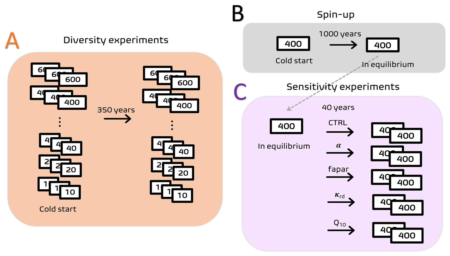
Figure 3 Experimental design used for the exploration of the behaviour of JeDi-BACH in the present study. Each box represents a separate simulation, the number indicates the the potential diversity used in this simulation. Panel (A) illustrates the setup of the “diversity experiments” described in Sect. 4. Their aim is to explore how simulation results depend on the level of potential diversity. In the “sensitivity experiments” (C), described in Sect. 5, the dependence of model results on parameter variations is analyzed (parameters indicated over the arrows; compare Tables 2 and 3). While for the diversity experiments a cold-start is performed, the sensitivity experiments are preceded by a spin-up simulation (B).

The aim of a spin-up simulation is to obtain a stationary state. Only by starting experiments from such a well defined reference state it is assured that when using different configurations in the subsequent simulation experiments, any differences in the simulation results can be attributed unequivocally to differences in these configurations. A spin-up doesn't need particular initial conditions, a cold-start will do. For JeDi-BACH a spin-up has reached a stationary state once (i) the selection of species by environmental filtering has largely come to a halt, (ii) key variables of terrestrial/global climate have reached except for fluctuations a constant value, and (iii) a drift in the size of the biomass carbon pools reached a tolerably small value.

The model set-up used for the experiments is in all cases the same: SSTs and SICs, anthropogenic aerosol optical properties, ozone, greenhouse gases, and the solar irradiance forcing are prescribed as AMIP forcing¹ (Gates et al., 1999). During the 1000 years of spin-up, the AMIP data from 1945 to 1974 is applied cyclically. For more information see Sect. 3.1.

For initially empty storage pools, many PGSs would die already early during spin-up. Therefore we initialize the PGSs with a small amount of carbon in the storage pools. In this way, the PGSs have a higher chance of surviving weather fluctuations during their early stage of development. Figure 4 shows exemplarily the convergence towards a stationary state for a 1000-year spin-up with 400 randomly sampled PGSs after a cold start. The left panel shows the percentage of the land grid boxes for which the total biomass from all six JeDi carbon pools changes per decade by less than 5 % and 10 %. Similarly, the right panel displays for the same spin-up simulation the development of the percentage of land grid boxes where the total number of surviving strategies changes per decade by less than 5 % and 10 %. The environmental filtering of strategies is initially rather vigorous and comes almost to a halt after 200 years of simulation. The biomass carbon needs longer to equilibrate: the filling of carbon pools slows down considerably after 350 years of simulation, but it needs another 250 years until the remaining small trend is smaller than the natural fluctuations in the filling and emptying of the pools – these fluctuations are the reason why the considered percentage of land grid boxes must always stay smaller than 100 %.

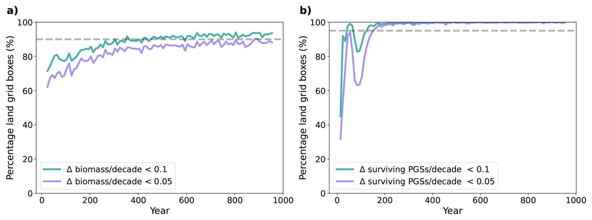
Figure 4 Example for convergence towards a stationary state during spin-up. Shown is the percentage of land grid cells where during spin-up total plant biomass (a) and total number of surviving strategies (b) changes per decade by less than 0.1 % and 0.05 %. Grey dash lines mark the 90 % level (Δ: difference). The data stem from a spinup simulation with a potential diversity of 400 randomly sampled PGSs. For more details see text.

Such a 1000-year coupled simulation with 400 PGSs using 32 nodes (equal to 768 CPUs of the supercomputer MISTRAL of German Climate Computing Centre (Deutsche Klimarechenzentrum, DKRZ)) needs at least 50 d to complete. This quickly adds up to a few months if the administrative time (i.e., queuing time until actual execution) is also considered. This lengthy process considerably challenges not only model testing during development but also future experimentation with this model. In this regard, we have future applications also developed a spin-up procedure using a combination of offline and fully coupled simulations that speeds up the whole process.

4 Dependence of ecosystem functions and climate on plant trait diversity

JeDi-BACH has been developed as a tool to study how biodiversity affects climate. That biodiversity affects climate is expected (see e.g. Begon et al., 1999, p. 917; Díaz et al., 2007) but not well explored. Hence one purpose of this chapter is to demonstrate by a sequence of simulations spanning from low to high diversity that indeed JeDi-BACH reveals indications for such an effect of biodiversity on climate. Similar sequences of experiments have been performed with other JeDi-DGVMs, but these studies focused on the effect of biodiversity on ecological functioning. Hence another purpose of this chapter is to investigate to what extent we recover these published results to gain confidence in the proper behaviour of our new JeDi variant.

4.1 Diversity experiment setup

To study the effect of diversity, we use a sequence of simulations performed in a coupled setup at seven levels of potential diversity (see definition in Sect. 2.1.2), namely with 10, 20, 40, 100, 200, 400, and 600 sampled plant growth strategies (PGSs). Each level comprises three ensemble members that were initiated with a different set of randomly sampled PGSs. By our experience, trees survive environmental filtering less often than grasses. Therefore, we constructed the sets of randomly sampled PGSs such that they contain slightly more trees (about 60 %) than grasses (about 40 %). The trait parameter values t₁, t₂, ..., t₁₅ (see Table B3) of each set are generated by Latin-hypercube sampling as described in Sect. 2.1.3. All experiments were configured with the same AMIP-type forcing as used in the coupled spin-up procedure (see Sect. 3.3). A total of about 350 simulation years was conducted for all ensemble members beginning from a “desert world” (cold start), meaning that all terrestrial grid cells grow vegetation from scratch. Due to limited computational resources, the maximum number of potential diversity was set to 600. The last 60 years of simulation results of each ensemble member are used for analysis. Antarctica, Greenland, and oceanic surfaces are excluded from the analysis.

4.2 Comparison of simulation results for different levels of potential diversity

To get a first impression of how actual diversity varies with the level of potential diversity, we compare in Fig. 5 the results from the low and high ends of our sequence of experiments. To make simulated actual diversity comparable across the different levels of potential diversity at which the experiments were performed, the plot shows actual diversity normalized by potential diversity. We call this quantity “relative diversity”:

$$\begin{array}{}\text{(52)}& \text{relative diversity}:={\displaystyle \frac{\text{actual diversity}}{\text{potential diversity}}}.\end{array}$$

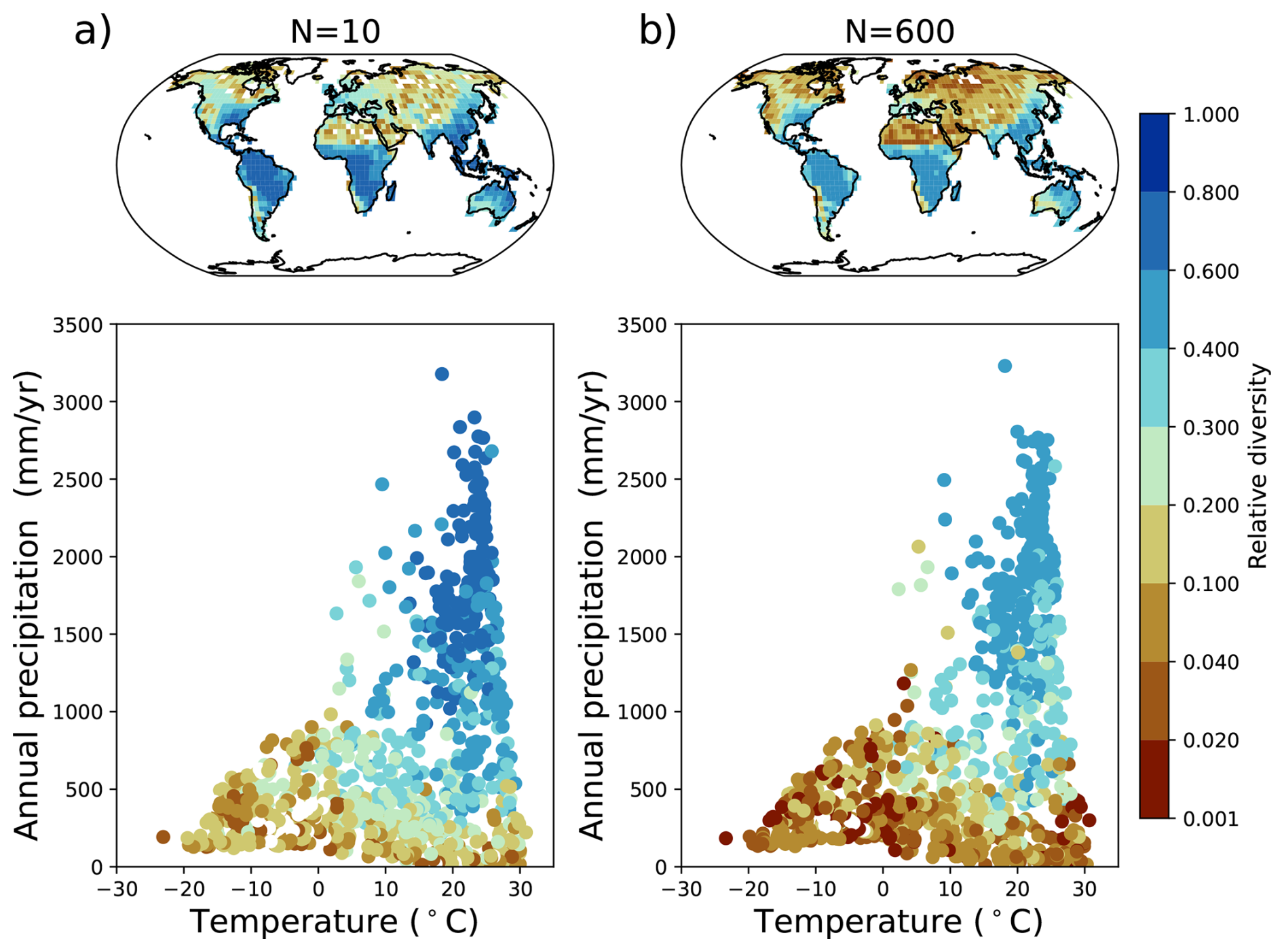
Figure 5 Ensemble mean relative diversity (see Eq. 52) for simulation experiments with a potential diversity of (a) N=10 sampled strategies and (b) N=600 sampled strategies. Results are shown in climate space, spanned by annual mean precipitation and annual mean surface temperature, where each dot represents a single grid cell. The insets show how these data are distributed geographically; at land grid cells shown in white all PGSs went extinct. The values shown are the ensemble mean of three simulations that we performed at each level of potential diversity, using for each simulation a different set of randomly sampled PGSs.

Note that relative diversity may as well be understood as the fraction of PGSs that has survived environmental filtering (“survival fraction”). To construct the plots of Fig. 5, we have calculated for each grid cell the mean of the relative diversity across the ensemble of three simulations performed for different sets of randomly generated PGSs. A high relative diversity (value ∼1) implies a hospitable environment, as in this case most of the initially sampled PGSs have survived environmental filtering.

Comparing the maps in Fig. 5, both simulations show roughly a similar global pattern: Relative diversity primarily captures the general latitudinal gradient of observed biodiversity patterns (compare e.g. Barthlott et al., 1996). In climate space, diversity declines with annual mean temperature and precipitation, where humid tropics have the highest diversity and dry or cold regions (e.g., Sahel, polar regions) have relatively low diversity. Due to substantial precipitation biases from the atmospheric model operating at a relatively coarse resolution (see Fig. A1), the current untuned version of JeDi-BACH tends to overestimate diversity in subtropical regions, where precipitation is overestimated, and underestimate diversity in the Eurasian region, where precipitation is underestimated.

Another difference between low and high diversity simulations concerns the regions that are not colonized by vegetation, which are much larger in the low diversity simulation (see e.g. the white areas in central Eurasia). This difference arises because the probability that a set of 10 PGSs randomly sampled from trait space contains strategies that survive in all kinds of climate is less probable than for a set of 600 randomly sampled PGSs (compare Sect. 3.2). Therefore, for low diversity simulations it is more likely to have larger non-vegetated areas (bare land).

Following Pavlick et al. (2013), we next investigate how relative diversity develops along the whole sequence of our diversity experiments. Calculating as for the previous figure for each grid cell the mean of relative diversity across all three ensemble members, we have visualized in Fig. 6a for each level of potential diversity the global distribution of these values in the form of a box-and-whisker plot. Obviously, the distributions stabilize with increasing potential diversity: The median values decrease from 10 to 40 sampled strategies and then become fairly stable above 100 sampled strategies. Both the median and the interquartile range become similar with increasing potential diversity. This similarity again implies that in our model world environmental filtering generally results in similar diversity patterns and gradients worldwide, independent of the total number of sampled strategies – which is indeed expected because the large-scale climate patterns should be very similar at the different diversity levels despite the interactive coupling between land and atmosphere present in our simulations (see Sect. 4.4 below). In this respect, our model behaves very similar to JeDi-DGVM simulations by Pavlick et al. (2013, Fig. 10a), except that their percentage of surviving strategies (which is the other meaning of relative diversity) converges at high diversity to only half of our value. The reason for this difference is not clear, it may be the different climates (they use observed climate, while ours is simulated). Other explanations could be differences in the implementation of land physics, or that we use an explicit representation of grass PGSs in JeDi-BACH.

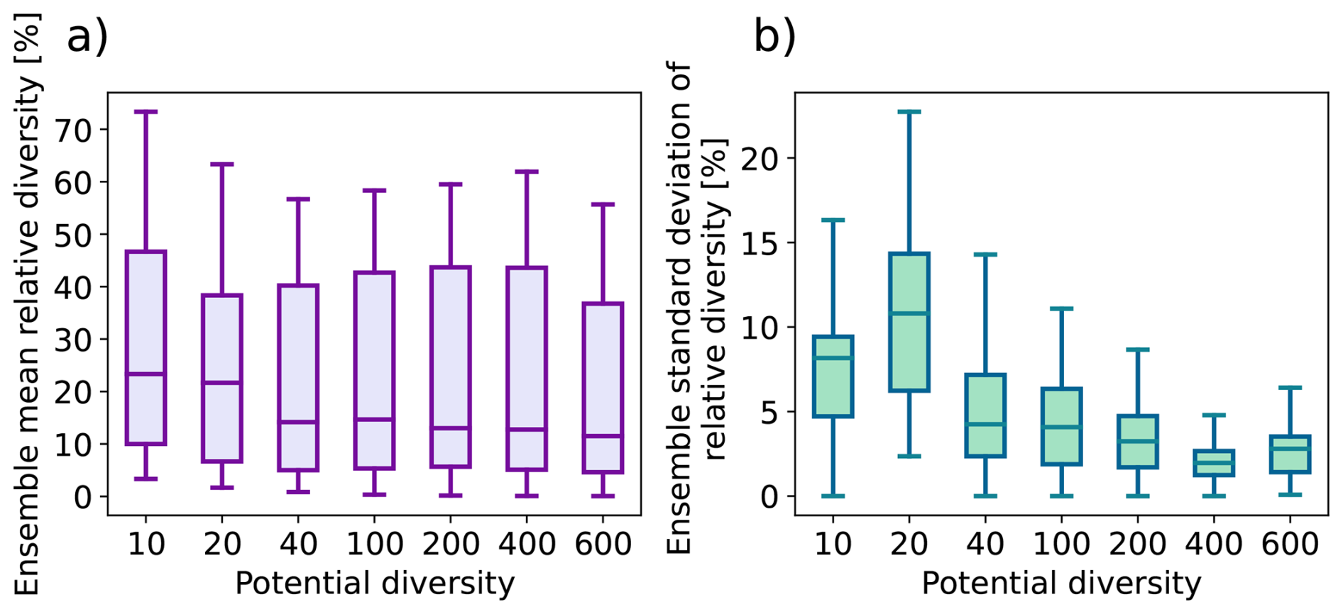
Figure 6 Box plots showing how the distribution of (a) ensemble mean and (b) ensemble standard deviation of relative diversity changes in our sequence of simulations performed for increasing potential diversity. For potential diversity 10 and 600 the box plots in (a) visualize the same set of ensemble mean values as in Fig. 5. The data underlying (b) have been obtained in the same way as for (a), except that instead of the mean, the standard deviation of the three ensemble values has been calculated for each grid cell.

Once more following Pavlick et al. (2013), we visualize in Fig. 6b the worldwide spread in the ensemble standard deviation of relative diversity. Towards high potential diversity the interquartile range substantially decreases, meaning that relative diversity gets very similar between the different ensemble members in a grid cell. The reduction in the ensemble spread also means that the fraction of PGSs surviving environmental filtering converges at almost every land grid cell so that simulation results get at high potential diversity rather independent of the initial set of randomly sampled traits. Also in this respect, our new JeDi implementation behaves very similarly to that of Pavlick et al. (2013, Fig. 10b).

4.3 Convergence towards functional similarity at high diversity

So far we found for large diversity a convergence in the fraction of surviving PGSs. In this section, we show that also community structure and functioning converge. The term “community” is used here for the collection of PGSs in a grid cell in connection with the concept of biomass scaling (Sect. 2.9). By this biomass scaling, the collection of PGSs is given a structure: in terms of biomass and share of exchange fluxes with the atmosphere some PGSs thereby get more dominant than others. The weight given to each PGS is calculated from its biomass density in relation to all other PGSs in a grid cell (see Eq. 49) and is interpreted within JSBACH as the cover fraction of a PGS. Employing this concept of weighting, we demonstrate in this section that the communities of PGSs in a grid cell get structurally and functionally very similar at high diversity.

Such a convergence is already visible at the most fundamental level of diversity of JeDi, namely at the level of individual traits. This is seen exemplarily in Fig. 7 for the trait t₃ which determines the parameter T_start, specifying the temperature at which the growth season of a PGS starts (see Eq. 13). The figure shows for the various levels of potential diversity the global distribution of the community weighted means CWM(t₃) of the alive tree PGSs (compare Eq. 51) separately for each of the three ensemble members. At low diversity these distributions look very ragged because in this case at many grid points only a single tree PGS survives meaning that CWM(t₃)=t₃ so that the distribution has non-zero values mostly at exactly the randomly sampled t₃ values (note that for every grid box, the same set of initial trait values is used). While the three distributions are very dissimilar at low diversity, they converge towards a common distribution at high diversity.

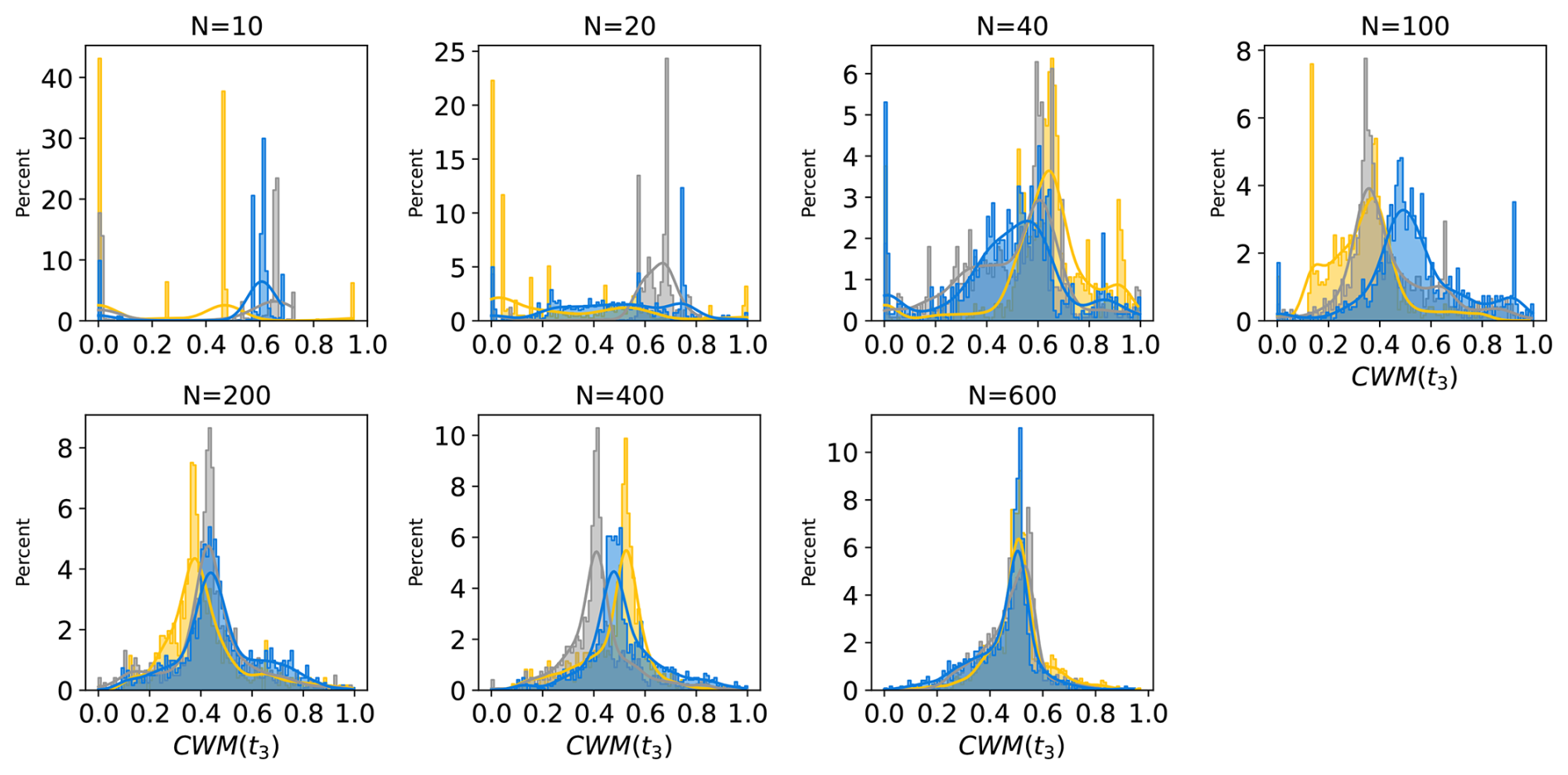
Figure 7 Convergence of the global probability distribution of the trait value t₃ of tree PGSs with increasing potential diversity N. This trait parameter t₃ specifies the temperature T_start at which the growth season starts (see Eq. 13). To obtain these distributions, we calculated for each land grid box the community-weighted mean CWM(t₃) of the tree strategies that survived environmental filtering. The distributions in the figure then depict the fraction of all land grid boxes (“density”) having a particular value CWM(t₃). The distributions are calculated separately for each of the three ensemble members (depicted by different colors). Note the convergence towards a single distribution at high potential diversity which indicates independence from the set of initially sampled t₃ values.

This convergence is not only seen for trait t₃, but for all traits. Instead of demonstrating this for each trait separately, we consider in Fig. 8 for the alive PGSs the statistics of the ensemble standard deviation across all CWM trait, but separately for trees and grasses because of the different number of relevant traits (see Sect. 2.1.1). To see how strongly these CWM trait parameters differ between the different ensemble members, we calculated for each grid cell the standard deviation of the set of three ensemble members and plotted the distribution of these values. For both grass and tree strategies, the median values and the inter-quantile ranges generally decrease with diversity. Accordingly, not only individual CWM trait values, but the whole set of trait values becomes similar with increasing diversity across all ecosystems worldwide.

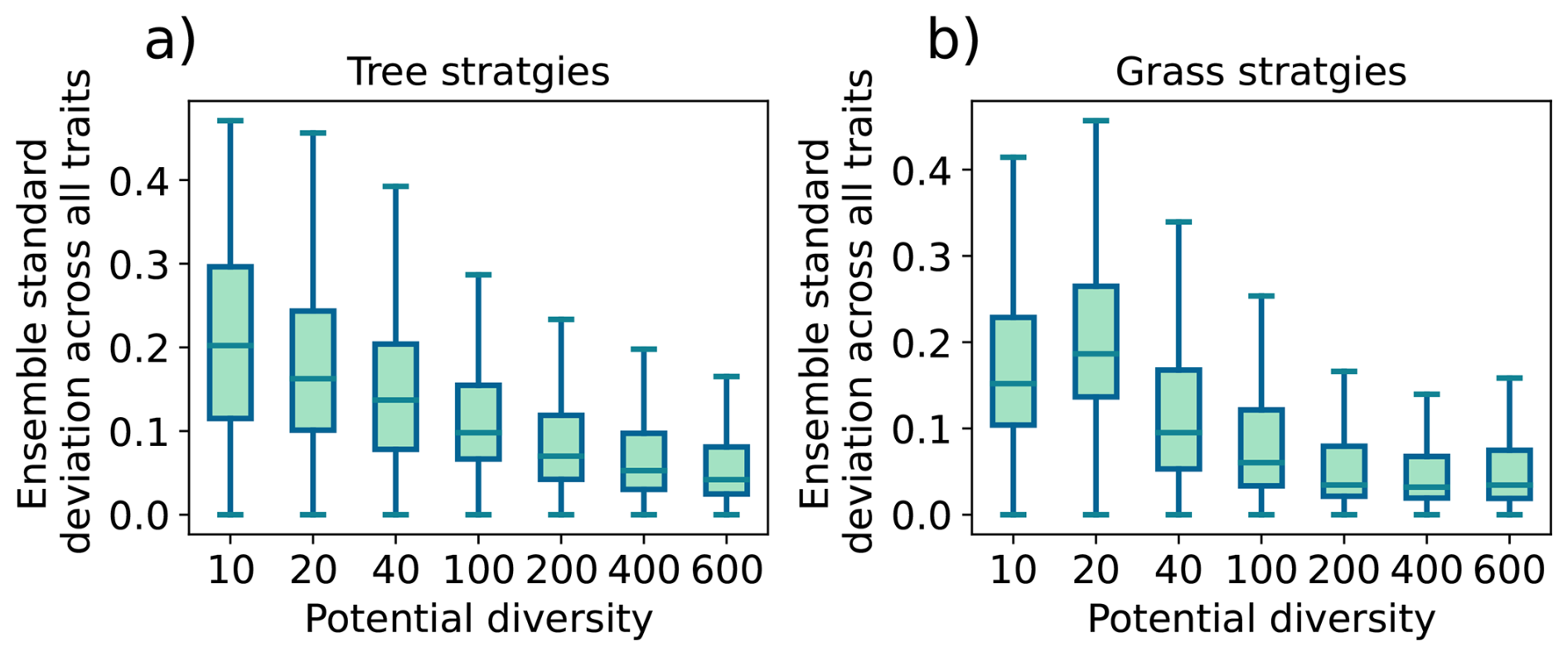
Figure 8 Convergence of the ensemble spread of the combined 15 trait values towards high diversity for (a) tree PGSs, and (b) grass PGSs. These figures have been obtained by first calculating for each trait and each vegetated grid cell their standard deviation (“SD”) across the three ensemble members, and then pooling all these SD values into a single data set. The displayed box plots of these data show how abundant these SD values are globally across all traits and all vegetated grid cells.

This convergence at the most fundamental level of biodiversity has an important consequence – we find that ecological function also converges with increasing potential diversity. We demonstrate this in Fig. 9 exemplarily for the net primary productivity (NPP), global vegetation biomass, and evapotranspiration (ET). The three upper panels demonstrate that their values get very similar towards high potential diversity. In the lower panels, it is seen that also the global distribution of the ensemble spread gets very similar at high potential diversity. For NPP, similar plots have been published by Pavlick et al. (2013) for simulations with their JeDi implementation. While in our simulations NPP decreases with increasing potential diversity, in their simulations NPP increases. Possible reasons for this different behaviour are discussed in the final discussion section below.

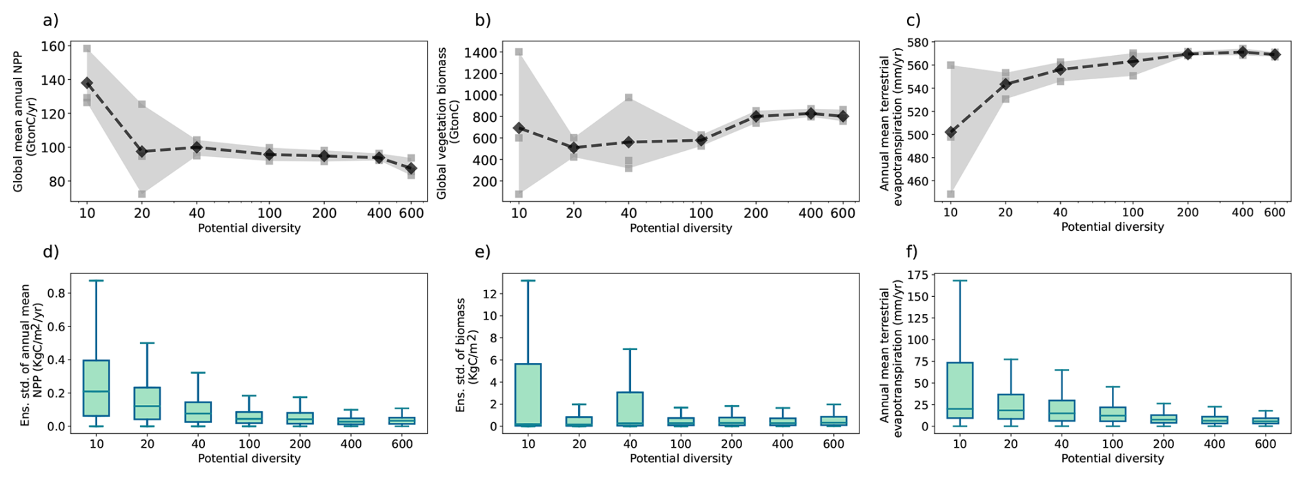
Figure 9 Independence of ecosystem functioning from the initial set of plant growth strategies at high potential diversity demonstrated exemplarily for global annual NPP, global vegetation biomass, and annual mean terrestrial evapotranspiration (ET). In panels (a), (b), and (c), we show this for their global values, plotted separately for each of the three ensemble members (grey squares) – obviously, their values converge towards high diversity, even though the underlying sets of trait values (of strategies) are different. (The black diamonds connected by a dashed line depict the mean of the three ensemble values.) A similar conclusion can be drawn from the box plots in panels (d), (e), and (f) that depict the global distribution of the “spread” between the three ensemble members – obviously, these distributions get rather similar at high diversity. The box plots are obtained by first calculating separately for each of the three ensemble members for each land grid cell a 60-year mean of the CWM of NPP, biomass, and ET. Then, the standard deviation (SD) of the three ensemble members is calculated at each land grid cell. Last, each box plot, interpreted as “spread”, collects all the SD values over land at each potential diversity.

The plots in this section demonstrate that towards high potential diversity the distribution of the randomly sampled trait values defining the set of PGSs gets increasingly irrelevant. This may be explained analogous to the explanation of the formation of niches as introduced by Hutchinson (1957) (see also Begon et al., 1999, Sect. 2.12, and Schulze et al., 2019, Sect. 20.2.3.2): Imagine that the trait parameters form a multi-dimensional trait space (trees: 15 dimensional; grasses: 13 dimensional; see Sect. 2.1.1). Each PGS represents a certain combination of trait values, i.e. each PGS is a point in this multi-dimensional space. If a plant strategy successfully survives in a particular environment, it must have developed specific trait combinations to cope with the respective environment. Hence, for a given environment, there are regions in the multi-dimensional trait space where the respective PGSs perform better in the sense of biomass production than those from other regions. There may be even islands with particularly high biomass. Now, with increasing potential diversity, i.e. with an increasing number of PGSs sampled randomly from this trait space, the probability increases that the set of sampled PGSs contains some from such high biomass islands. The PGSs from these islands will then dominate the others in terms of biomass weighting, seen as a well defined peak in the distribution of biomass weighted traits. Moreover, at sufficiently high potential diversity, any set of PGSs will contain some PGSs from this island, which explains why for different ensemble simulations, i.e. for different sets of PGSs, the distributions and also the related ecosystem functions get very similar. In principle, there could be several such islands, of which the case N=400 in Fig. 7 may be an indication. But at the even higher potential diversity N=600 all three simulations apparently have the same trait distribution, being an indication for only a single high biomass island. Accordingly, we think that the presence of only a single island of high productivity in the multi-dimensional trait space of JeDi explains the convergence of ecosystem function found in our simulations.

4.4 Convergence of terrestrial climate for high diversity

The aim underlying the development of JeDi-BACH is to obtain an instrument for the investigation of the effect of biodiversity on climate. Hence, to demonstrate that the work invested in model development has been worth its effort, we further investigate here the sequence of simulations performed for different levels of potential diversity, but focusing now on the dependence of climate on potential diversity.

In the previous section, it was seen that towards high potential diversity, the community structure resulting from environmental filtering gets rather independent of the initially chosen set of trait values. In our coupled JeDi-BACH setup, the associated convergence seen in ecological functions (compare Fig. 9) happens while vegetation operates in close interaction with the surrounding physical environment. Accordingly, one can expect that in our simulations not only regional climates converge with increasing potential diversity, but also global climate.

And indeed, this is what we see in the simulations: Terrestrial 2 m air temperature (tas) and precipitation (P) converge towards a similar climate state with increasing potential diversity (see Fig. 10a–b). Interestingly, the convergence is towards a cooler and wetter climate state, seen especially in simulations with more than 100 randomly sampled strategies. For temperature and precipitation, this behaviour may be understood as a direct consequence of the increasing evapotranspiration (Fig. 9c): this increase leads to enhanced evaporation cooling and at the same time to a wetter atmosphere that triggers additional precipitation. Moreover, this particular climate state at high diversity seems to be extreme in the sense that it is as cool as the coolest low diversity state, and as wet as the wettest high diversity state. But one should be careful not to over-interpret this result: We have not fully analyzed this, but this tendency towards a wetter and colder climate at high diversity is likely a consequence of the biomass scaling. PGSs that are more successful in the accumulation of biomass are typically also more productive and have a higher rate of transpiration. Through biomass scaling, these PGSs contribute relatively more to the grid-cell-wide evapotranspiration, so that there is a tendency to maximize evapotranspiration. While this is not implausible behavior, such behavior may not apply in general everywhere, as survival strategies that minimize transpiration may be more successful (e.g., in dry climates). So, at the moment, one should take our simulation results only as a demonstration that the model might be an interesting tool to study how biodiversity may affect climate.

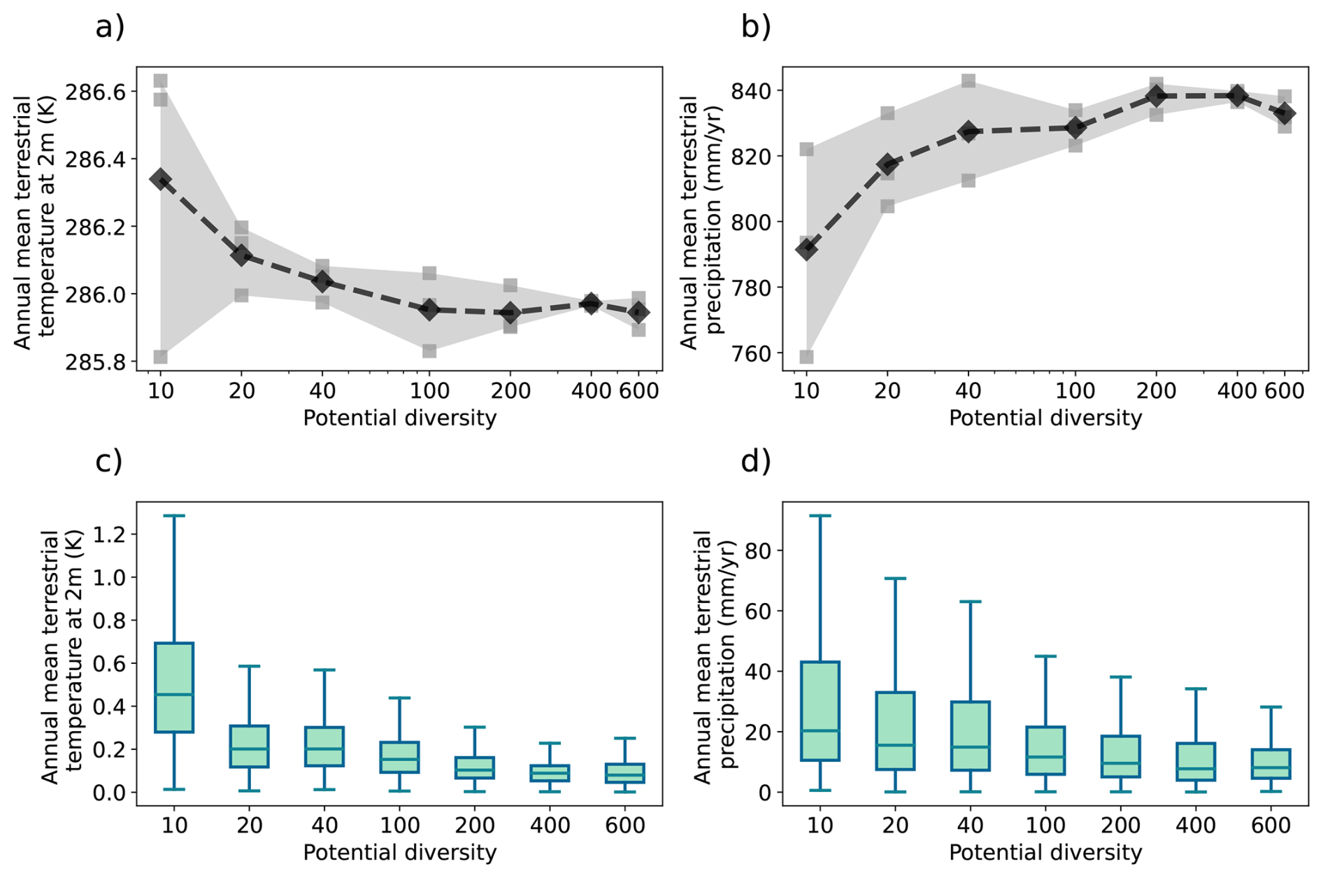
Figure 10 Convergence towards a unique terrestrial climate with increasing potential diversity independent from the initial set of plant growth strategies. This is demonstrated here exemplarily for (a) 2 m air temperature and (b) precipitation. Technically, the box plots have been prepared similarly to those in Fig. 9.

This behaviour seen in global climate variables is indeed a consequence of convergence at the regional scale: For the two climate variables considered here, this is demonstrated by the box plots in Fig. 10c–d. To obtain these plots for each grid cell their spread between the three ensemble members has been calculated as standard deviation and the plots show how this global set of spread values is distributed. Obviously, towards high potential diversity these distributions narrow down to a common distribution with small spread values, meaning that the climate gets even regionally similar between the three ensemble members.

The large variability observed in the low diversity simulations may be attributed to the large disparity in the CWM traits among ensemble members in low diversity simulations (see Fig. 8). These divergent ecosystem compositions result in distinct regional climates among the different ensemble members. Such a high sensitivity of climate to ecosystem composition observed in the low-diversity simulations is similar to the high sensitivity on the details of the representation of vegetation reported in previous PFT-based climate simulation studies (Groner et al., 2018; Verheijen et al., 2013; Betts et al., 2004; Cox et al., 2004; Huntingford et al., 2008): By our experience with this new JeDi-BACH model, we argue that because only a handful of PFTs is prescribed over land, changing land surface characteristics or plant properties may substantially modify regional climates. If so, the high sensitivity reported in PFT-based modeling studies likely stems from the poor representation of ecosystem complexity inherent to the PFT approach.

Note that by the JeDi-BACH simulations presented here – to our knowledge – for the first time a systematic effect of potential biodiversity on climate has been demonstrated. It is well known that regional climate is affected by the local type of vegetation via various interactions between vegetation and the lower atmosphere (see e.g. Shukla et al., 2019, chapter 2). But not only the type of vegetation, but also its diversity plays a role. This biodiversity-climate interaction could so far only be hypothesized because field experiments seem unsuitable (too small to have an effect on climate), and appropriate simulation models were missing. Hence, with the development of JeDi-BACH this gap has now been closed.

To conclude this chapter, it may be noted that from a technical point of view the observed convergence in ecological functions and climate means that JeDi-BACH reliably produces a robust terrestrial climate as long as a sufficient number of plant growth strategies is simulated. This means in particular that simulation results are independent of the choice of the initial set of sampled strategies. Hence, only at low potential diversity one may tune climate and ecosystem functions by a suitable choice of PGSs. The tunability of JeDi-BACH by a suitable choice of JeDi model parameters is the topic of the coming section.

5 (Un-)Tunability of climate

To best match the known state of the Earth’s climate system, tuning of model parameters is an important step during the development of a reliable climate model (Mauritsen et al., 2012). Tuning is necessary because models contain simplified process representations (called “parametrizations”) involving non-measurable parameters whose values must be adjusted by hand. In particular, terrestrial climate depends on how vegetation is represented in models (Groner et al., 2018; Brovkin et al., 2003, 2009), implying that model simulations are prone to subjective decisions hidden behind model-tuning. One essential idea underlying the JeDi-modeling approach is to use environmental filtering to obtain climate-adaptive plants so that values of parameters arising in the representation of vegetation – the trait values – need not be chosen by hand to tune the model (as in the PFT approach) but are selected by the model itself during simulation. In this way, the number of subjective parameters is largely reduced.

Nevertheless, quite a number of parameters remain that could be used for tuning. Previous JeDi-series models have demonstrated that the JeDi-modelling concept is able to capture several biogeo-physical and -chemical properties of vegetation fairly well compared to PFT-based models (Pavlick et al., 2013; Rius et al., 2023). Which parameters were used – if at all – to achieve this result has not been reported, although it would be interesting to know for future model development. The new aspect of our model JeDi-BACH is its interactive coupling with climate. In this chapter, we focus on how sensitive is terrestrial climate to vegetation parameters. For this purpose we selected a number of vegetation parameters and conducted a series of sensitivity experiments to assess how model results depend on their values. Because simulations with JeDi-BACH are rather costly, we restricted our investigation to only four parameters, namely those listed in Table 2. All chosen parameters qualify as potential tuning parameters because their values are only inadequately justifiable by observations. In addition, the selection of these parameters was guided by our expectation that their values are particularly influential concerning vegetation behaviour and may thus also have a considerable effect on climate. Finally, we choose in particular fapar and κ_rd because these are newly introduced parameters that have no counterpart in previous implementations of JeDi so that the performed sensitivity simulations serve also to test their proper functioning.

Table 2 Description of the four parameters selected for the sensitivity experiment.

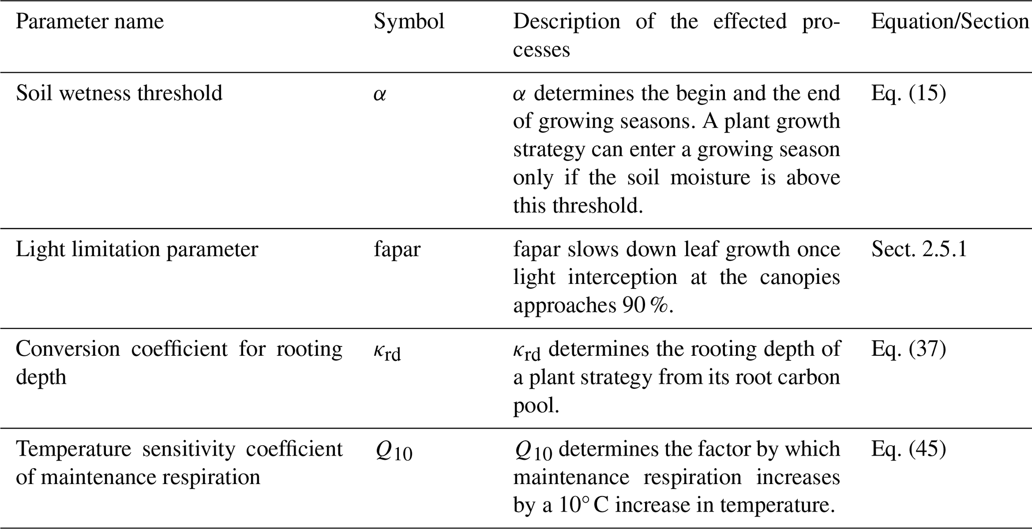
To our surprise, these simulations revealed that – at least for the chosen parameters – standard parameter tuning is meaningless due to compensation mechanism emerging from the particular way vegetation is modelled in JeDi: The active selection of new dominant strategies counteracts parameter changes. This leads to robust ecosystem functioning making conventional tuning useless. Thereby the simulation study presented in this chapter not only highlights one great advantage of JeDi-BACH in featuring more biosphere-like ecosystem behaviour that is different from the traditional PFT-based vegetation models, but also sheds light on potential future applications of this new model concerning the investigation of the potential links between biodiversity, ecosystem resilience, and interactions with climate.

5.1 Sensitivity experiment setup

To investigate the dependence of climate on parameter changes, we conducted for each of the four selected parameters (see Table 2) two simulation experiments. Table 3 summarizes the experiment design with the chosen parameter values. We thus conducted in total nine simulations, including one control (CTRL) simulation. The aim is to compare the results of the sensitivity experiments with the CTRL simulation to obtain the order of magnitude of climate change. The parameter values used in the control simulation are those already used to investigate the dependence on potential diversity in the previous section. Ideally, a separate spin-up should be performed for each of the eight sensitivity experiments. However, such a procedure is not feasible in view of the computational resources needed. Instead, all sensitivity simulations are continued from one common spin-up simulation that is initiated with 400 randomly sampled strategies. The parameter values are chosen to be substantially different from those in the control simulation to observe a significant impact. Each simulation is conducted with only one parameter changed at a time. As with previous experiments, also the experiments here are carried out in an AMIP-type setup. The simulations are forced by prescribed SSTs, SIC, greenhouse gasses, and aerosols for 1979 to 2014 following the CMIP6 AMIP protocol (Eyring et al., 2016). We use the last 15 simulation years (2000 to 2014) of all nine simulations for the analysis. Ocean surfaces, Antarctica, and Greenland are excluded from the analysis.

Table 3 Values of selected parameters used in the various sensitivity experiments.

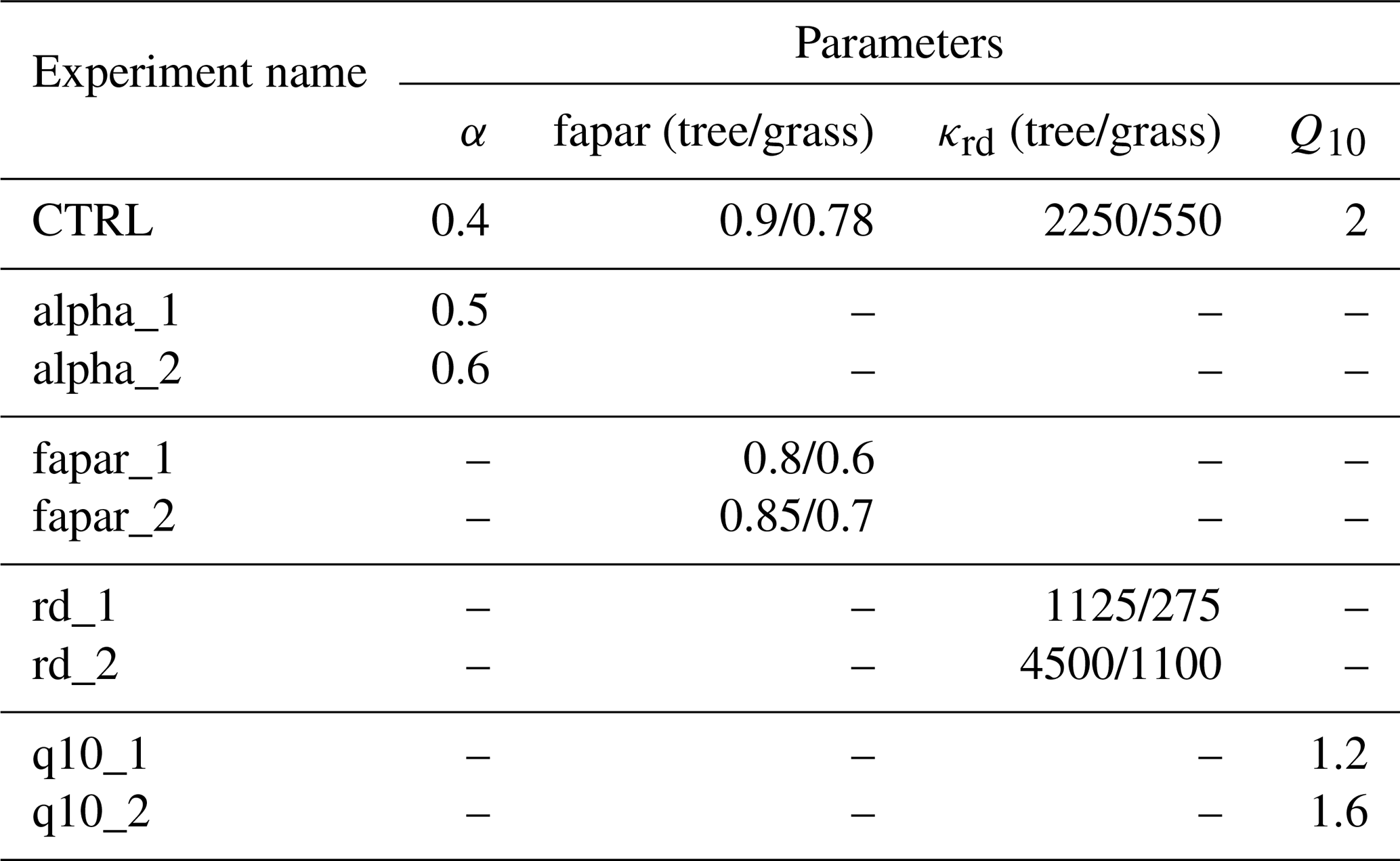
To demonstrate that indeed the chosen parameter values alter ecosystem function considerably, we list in Table 4 how strongly global annual NPP is affected by the parameter change in the different sensitivity simulations. In all cases one finds a clear signal in the relative change of NPP, being larger than 10 % for the strongest parameter change except for fapar where it reaches 6.5 %. Similar sizes are reached in other ecosystem variables (not shown) so that one should indeed expect that by the various interactions between ecosystems and atmospheric processes also climate is affected by these parameter changes. To what extend this is the case is discussed in the next section.

Table 4 Change in global net primary productivity (NPP) due to the changes in parameter values found in the different sensitivity experiments. For the chosen parameter values, see Table 3.

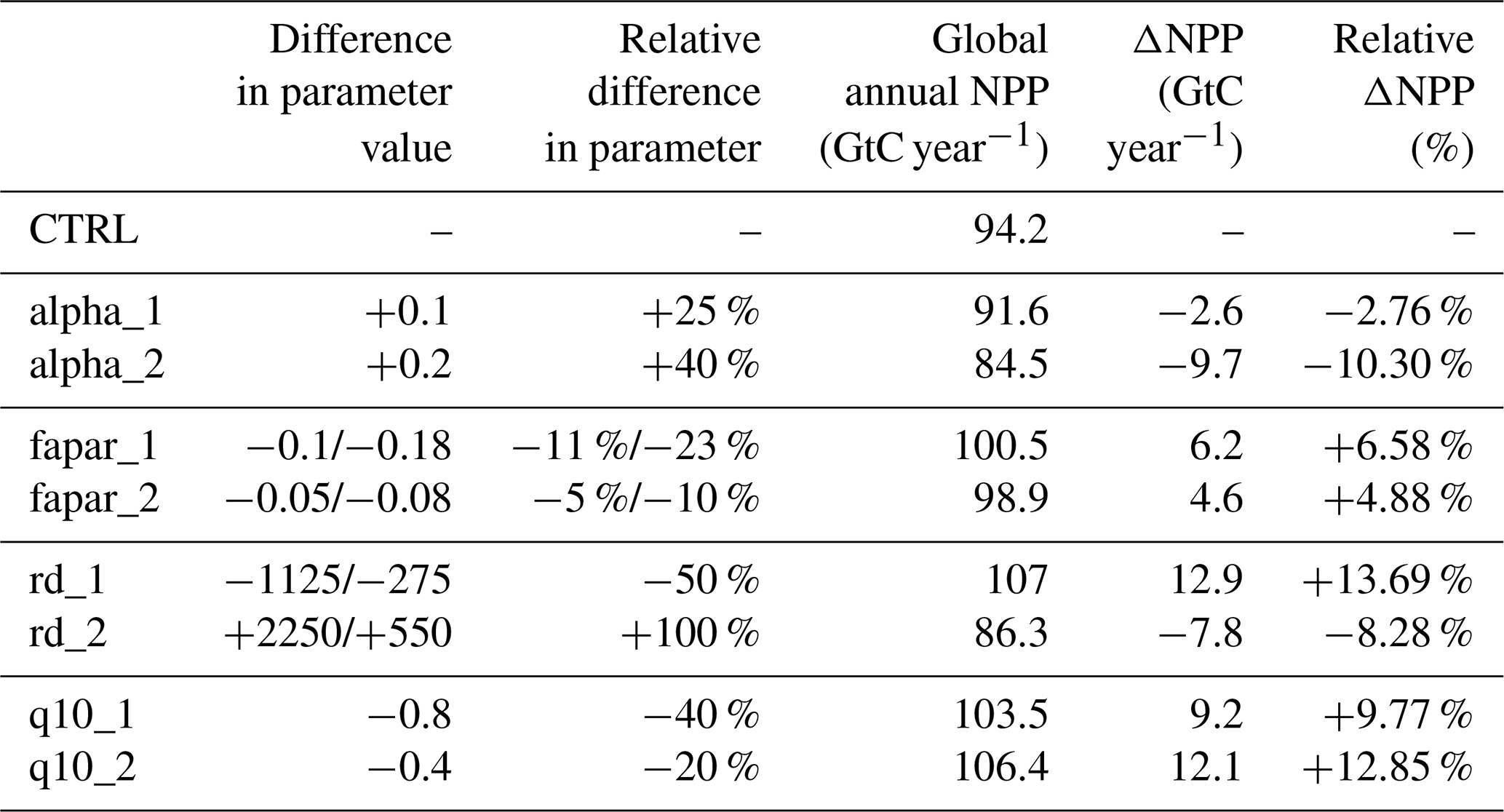
5.2 Sensitivity of terrestrial climate to changing parameters

To explore to what extent terrestrial climate is sensitive to changes in the four considered parameters, we compare here the eight sensitivity experiments (see Table 3) with the control (CTRL) simulation. As variables characterizing climate we consider in particular precipitation and temperature.

First, zonally averaged climate is considered (Fig. 11). Despite the differences in the parameter values, zonally averaged terrestrial temperature and precipitation found in the sensitivity experiments turn out to be nearly identical to that of the CTRL simulation. This is an indication that the large-scale atmospheric circulation remains generally the same regardless of parameter changes.

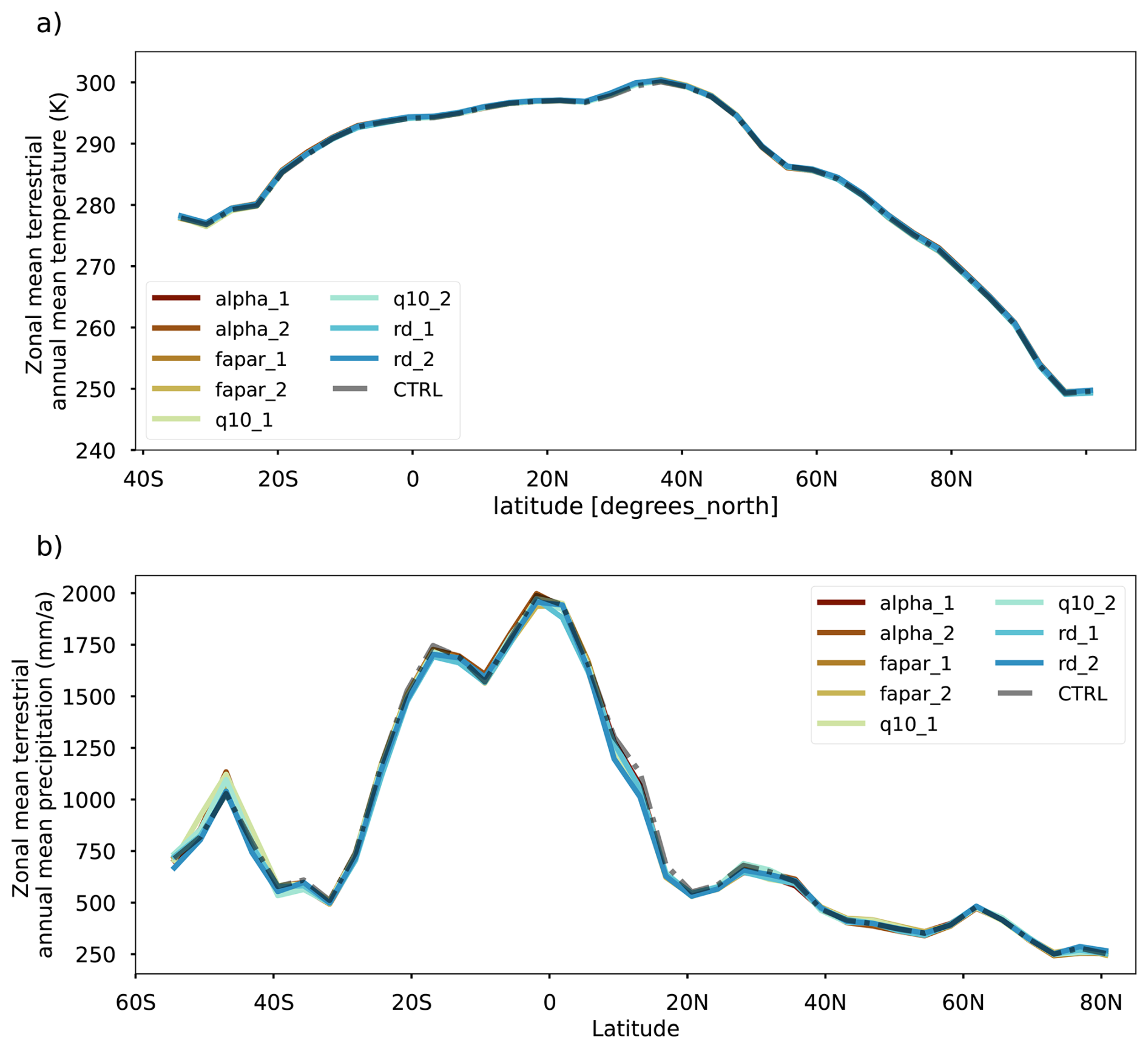
Figure 11 Comparison of the zonal mean climate over land between the control simulation and the eight sensitivity simulations (compare Table 3): (a) annual mean 2 m air temperature (K), (b) annual mean precipitation (mm year⁻¹). The values from the CTRL simulation are shown as grey dashed-dotted line.

To evaluate regional climate differences in more detail, we show in Figs. 12, 13, and 14 differences in temperature, precipitation, and evapotranspiration between the eight simulations and the CTRL simulation. The plots also show the statistical significance of the difference values according to a 5 % level in a Mann-Whitney test. Obviously, regional climate is statistically indistinguishable from the CTRL simulation in nearly all terrestrial regions. One of the few regions where climate depends on the considered parameters is the western Sahel (5 to 18° N; 15° W to 18° E). Compared to the CTRL simulation, all the sensitivity simulations depict a warmer and dryer climate there. In this region, all simulations except q10_2 show a significant increase in temperature, while two of them (alpha_2 and rd_2) show also a significant reduction in precipitation and evapotranspiration (ET) there. These two simulations (rd_2 and alpha_2) show the most intensive regional warming and drying, where annual precipitation is reduced by between 150–500 mm and air temperature increased by about 1–1.5 K. This drying and warming is consistent with a regional reduction in ET.

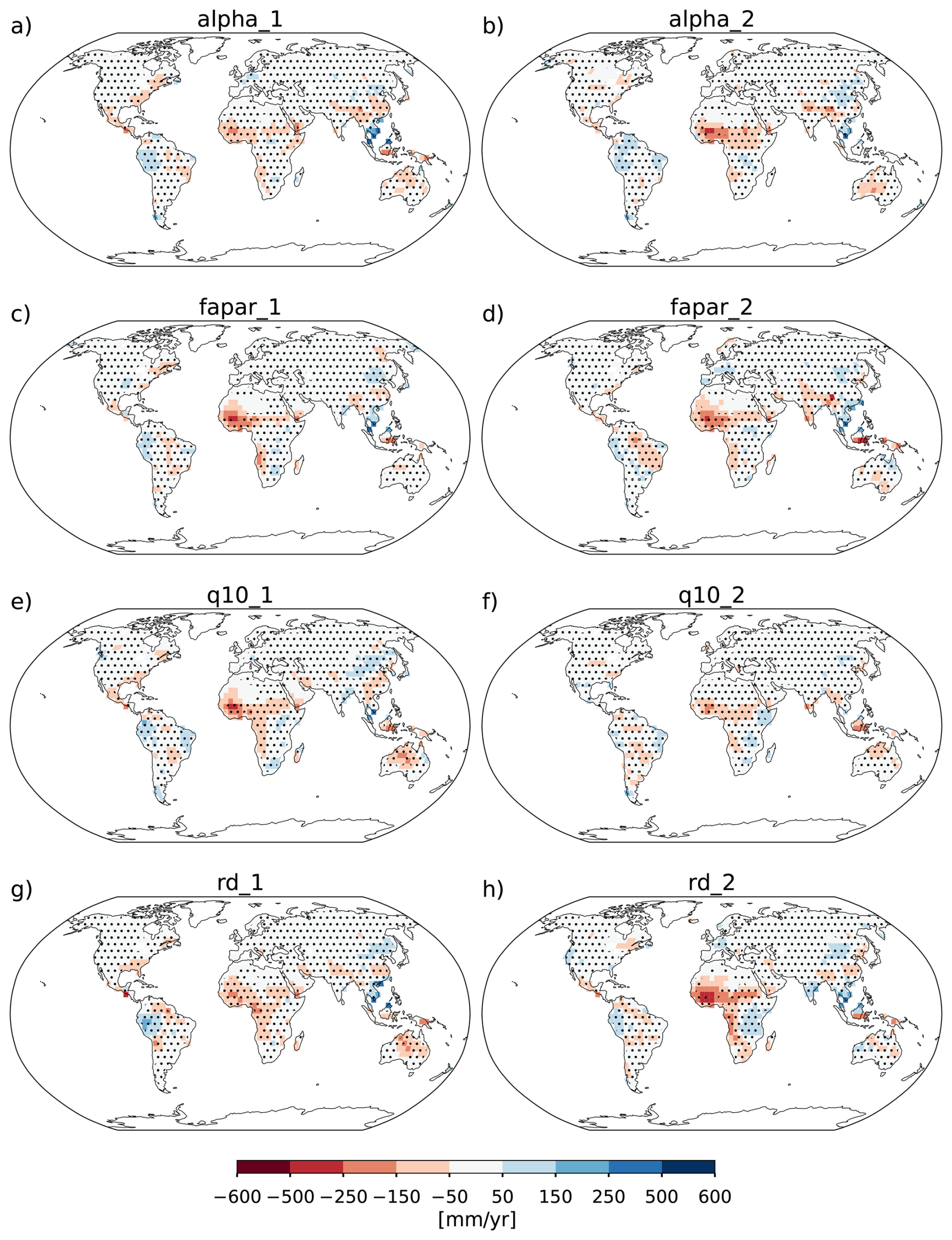
Figure 12 Difference of annual mean precipitation (mm year⁻¹) between each sensitivity simulation (see Table 3) and CTRL simulation. In grid cells marked with a dot the difference to the control simulation is statistically not significant according to a 5 % level in a Mann-Whitney test. Ocean surfaces and Antarctica are excluded from the analysis as they were prescribed with the same forcing data in all simulations.

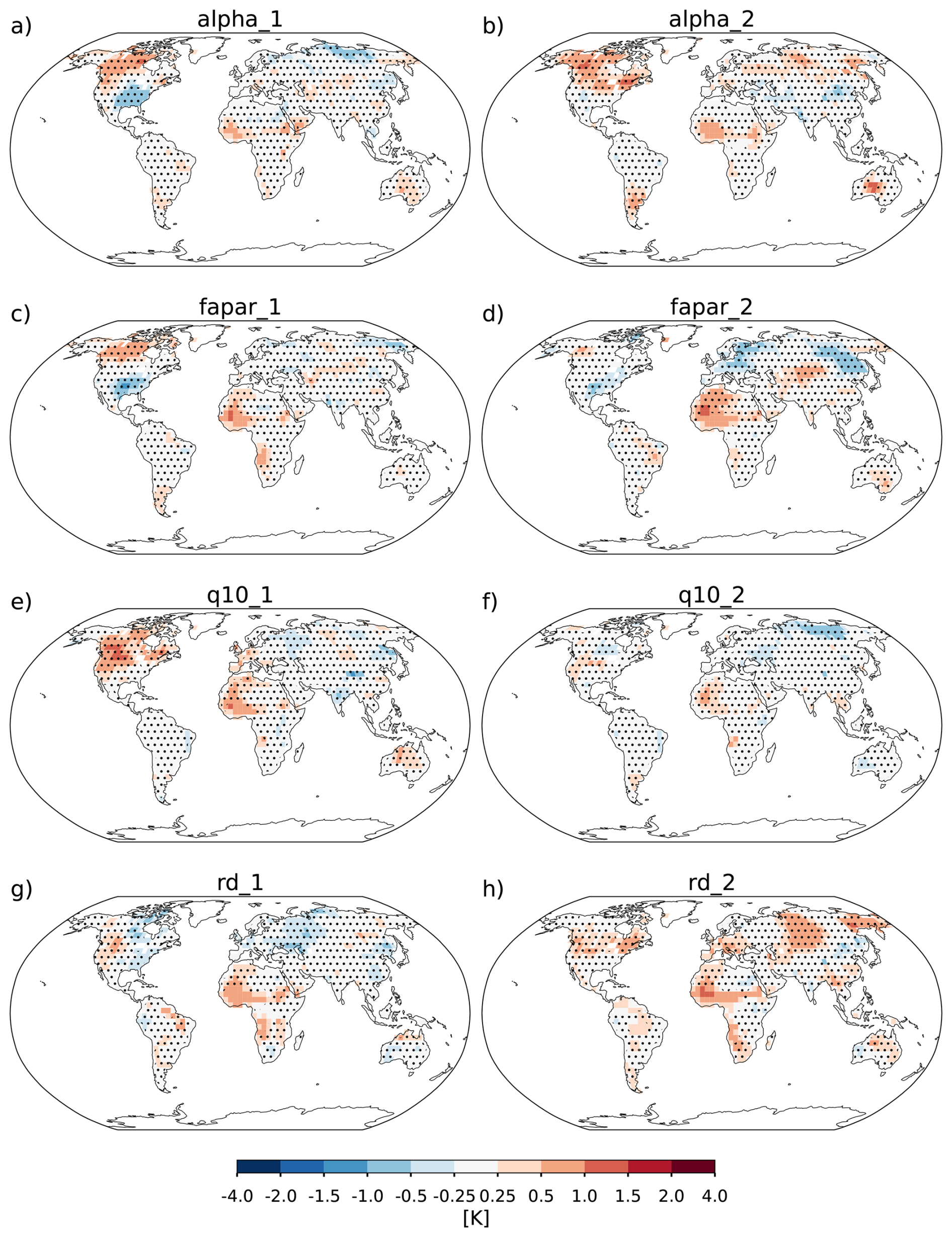
Figure 13 Difference of annual mean 2 m air temperature (K) between each sensitivity simulation (see Table 3) and CTRL simulation. In grid cells marked with a dot the difference to the control simulation is statistically not significant according to a 5 % level in a Mann-Whitney test.

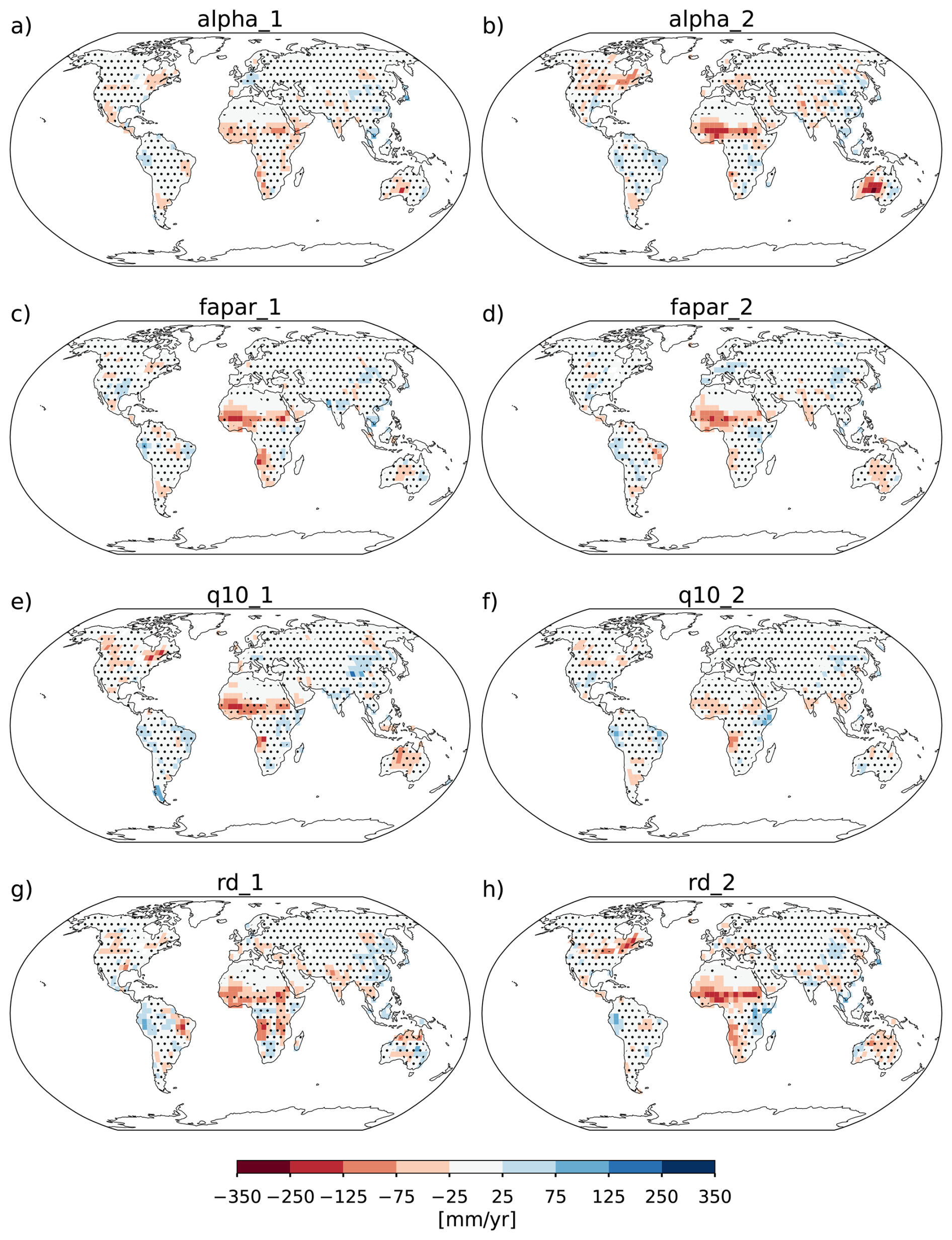
Figure 14 Difference of annual mean evapotranspiration (mm year⁻¹) between each sensitivity simulation (see Table 3) and CTRL simulation. In grid cells marked with a dot the difference to the control simulation is statistically not significant according to a 5 % level in a Mann-Whitney test.

It is well known that the western Sahel climate is dominated by the West African Monsoon: Southwesterly winds bring moisture from the Atlantic into the inner part of the western Sahel. Hence, one may suspect that the climate change in the Sahel may be related to changes in the large scale circulation pattern over North Africa. To assess this question, Fig. 15 shows exemplarily the difference in moisture transport between the alpha_2 and the CTRL simulation. One sees that the differences in moisture transport near coastal regions in western Africa are small compared to mean annual precipitation, implying that moisture transported from the Atlantic Ocean via west African monsoon circulation into North Africa is very similar in both simulations along the coast. Accordingly, the difference in the pattern of inland moisture transport seems to have an independent cause. This change in inland moisture transport points towards the southwest, meaning that transport into the inner part of western Africa is weakened (see the size of the arrows). The specific humidity also decreases (shown in red), consistent with the reduction in precipitation (Fig. 12a) and evapotranspiration (Fig. 14b). This behaviour may be explained by noting that in the alpha_2 simulation the threshold for soil moisture, determining where the growing period may start, is increased compared to the CTRL simulation. Accordingly, the growth period will typically start later so that in accordance with simulation results annual evapotranspiration is reduced. Therefore, the likely mechanism explaining the pattern seen in Fig. 15 over the western Sahel is not a change in the large scale circulation pattern, but a weakening of regional moisture cycling induced locally by a reduction in evapotranspiration.

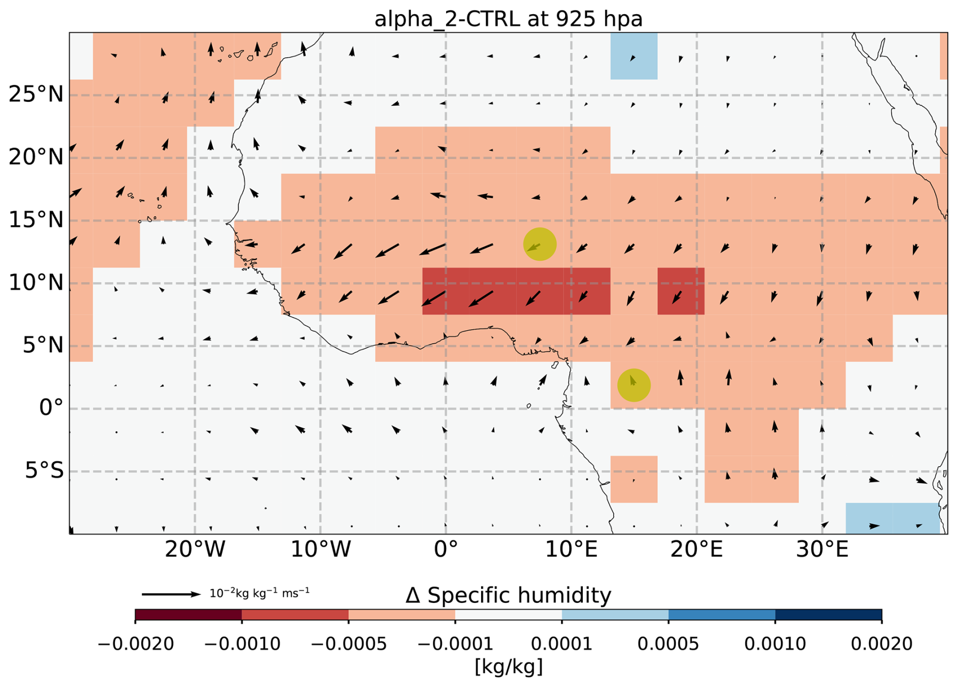
Figure 15 Difference of moisture transport at 925 hPa between the alpha_2 and CTRL simulation over the equatorial Atlantic. The difference in the specific humidity (kg kg⁻¹) is shown in color. The arrows show the difference in moisture flux, and their size indicates the magnitude of the difference. The moisture flux is calculated as the product of the wind field (m s⁻¹) and specific humidity at 925 hPa. The yellowish points mark the locations of the two selected ecosystems analyzed in Fig. 16.

Overall, the simulation results presented in this section show that for the four parameters chosen, climate is largely independent of their particular values. Because the choice of these parameters has been quite ad hoc, it has to be expected that similar results would be obtained also for other model parameters. If so, this has an important consequence for the process of model development: climate is not tunable by them. This does not mean that tuning of climate is generally impossible in a model like JeDi-BACH: The parameters chosen here to test the sensitivity of climate are insofar specific, as they control the ecosystem functioning. But there are many more parameters that control the land physics in JeDi-BACH. In the next section we will show that the likely reason for the parameter insensitivity is that the large number of PGSs in JeDi-BACH allows the ecosystem not only to flexibly adapt to environmental conditions, but also to modify them. This flexibility arises in the JeDi-component of JeDi-BACH, so that the un-tunability likely concerns only vegetation parameters, but not those of the model physics.

5.3 Shuffling in ecosystem composition as cause of climate insensitivity

In the previous section it was seen that a change in parameters had almost everywhere no effect on climate. Nevertheless, manipulating parameters does have an effect on ecosystem structure. In fact, shuffling in ecosystem composition (the exchange between dominant and subordinate strategies in an ecosystem) is the reason behind the robust climate in our sensitivity simulations. This is demonstrated in the present section by comparing ecosystem shuffling exemplarily between two locations, one in Congo where climate is unaffected by parameter change, and one in the western Sahel, one of the rare regions where climate shows an effect (see yellowish points in Fig. 15).

In JeDi-BACH, the dominance of a plant growth strategy in an ecosystem is proportional to its biomass (see Eq. 50), meaning that the “bigger” a PGS is, the more this strategy contributes to the interaction with the atmosphere. Accordingly, one can rank the dominance of strategies by their relative biomass. A shuffle in the ranking during a simulation indicates that the previously subordinate strategies (with lower rankings) outperform the previously dominant strategies (with higher rankings) so that they now occupy the upper rankings and have gained more relevance for the shaping of local climate.

The sensitivity experiments analyzed here start out from the control simulation. Therefore, a change in a parameter value is similar to a “disturbance” imposed on the ecosystems. Considering the alpha_2 simulation, where the threshold for entering a growing season becomes stricter with a higher value of α (changing α from α=0.4 to α=0.6), we show in Fig. 16 how the biomass ranking of the top 30 PGSs changes at the two considered locations (“Congo”, “Western Sahel”) as a consequence of the parameter change. The change in ranking is visualized by using grey lines to link the rank a PGS had in the CTRL simulation with the rank it assumes after the parameter change in the alpha_2 simulation. Obviously, at both locations a reordering of the ranking happens because some PGSs perform better while others perform worse with the changed parameters, leading to a re-organization of the community structure.

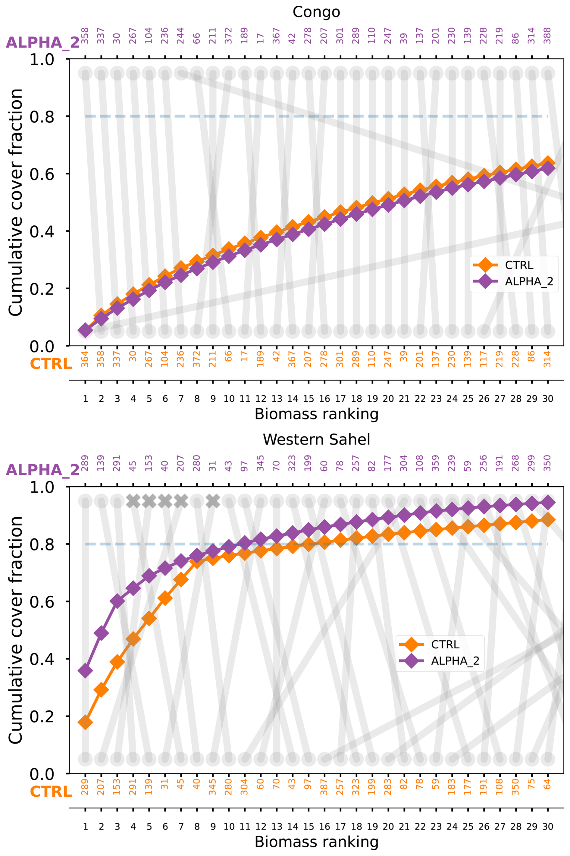
Figure 16 Change in biomass ranking from the CTRL simulation to the alpha_2 sensitivity simulation (compare Table 3) for a grid cell in Congo (top panel; 0° N, 15° E) and in the western Sahel (bottom panel; 13.125° N, 8° E) – see the location marks in Fig. 15 (yellowish points). The vertically arranged numbers on x-axes are the model-internal identifiers of the different PGSs for the CTRL simulation (bottom) and alpha_2 simulation (top). The PGSs are rank-ordered from high biomass (left) to smaller biomass (right). The grey lines linking identical PGSs show how its biomass ranking changes from the CTRL to the alpha_2 simulation. In the alpha_2 simulation of the Sahel case some of the PGSs have died upon the parameter change, in the plot these have been marked with thick crosses. The dead PGSs nevertheless show up in the ranking because the dead biomass is still around in the grid cell (see the discussion at the end of Sect. 2.10). The curves with the diamond dots show for the two simulations how much of the vegetated area in the grid cell is covered up to a particular PGS according to biomass weighting (compare Eq. 49).

Comparing the figures for the two locations, it is very obvious from the patterns of the grey lines that in the Congo case there is not much re-shuffling, while in the Western Sahel the community undergoes a strong re-organization, even some of the PGSs have died (see the thick crosses). The Congo community seems to be much more resilient: except for two strategies (#364 and #117) all others stay in the field of the 30 top ranked strategies, even their rank-order mostly remains, with only few swapping their places. Noting from the biomass curves in that figure that the contributions to biomass of the individual PGSs are rather small (the first 30 contribute only 60 % of the biomass), a failure of a few of them may not have much effect on the exchange with the atmosphere. Not so in the Sahel case: Already the first 10 PGSs make up almost 80 % of the biomass so that if one or more of them fail to cope with the new situation this must have a strong effect not only community structure but also on the interaction with the atmosphere. And this is exactly what happens in the Sahel: five of the first top ranked PGSs die out and a lot of re-ordering happens, indicating that the community at this location is much more sensitive to the parameter change than in the Congo. Note that this explanation for the sensitivity of climate to parameter change at the Sahel location is a regional one. But this is consistent with the conclusion from the analysis of the changes in moisture transport over North Africa in the previous section (compare in particular Fig. 15) indicating that climate change found there is likely not caused by changes in trans-coastal moisture import from the Atlantic, but by regional changes in Africa itself.

In summary, it is very likely that the results from the last section, namely the insensitivity of climate to parameter changes in most parts of the world and the exceptional sensitivity in the western Sahel, may both be explained by the ability or inability of the local ecosystems to compensate these changes by a re-organization of their community structure. At the Congo location the set of PGSs present in the CTRL simulation is rather redundant in the sense that a parameter disturbance leading to a deterioration in the fitness of individual PGSs can be well compensated by other PGSs. In contrast, at the Sahel location the set of PGSs present in the CTRL simulation is lacking potential for substitution of failing PGSs. This has been demonstrated here only for the alpha_2 simulation, but the question of redundancy depends only on the set of available PGSs at start of the parameter change, namely the set of alive PGSs in the CTRL simulation from which all sensitivity experiments started. This set of alive PGSs is different in different grid cells, but in each grid cell all sensitivity experiments thus inherit the same set of PGSs from the CTRL simulation so that concerning redundancy and the possibility to compensate for changes in fitness they should behave very similarly. This explains why, as seen in the previous section, in the different sensitivity experiments the regions without and with climate change are so similar. It doesn't explain why exactly in the western Sahel redundancy is so poor, this may be a peculiarity of the initial set of randomly chosen PGSs, i.e. we cannot exclude the possibility that with a different set of initial PGSs, or for a larger set of initial PGSs, also in that region climate would be insensitive to parameter changes.

6 Summary and conclusions

This paper provides a description of the implementation of the plant functional diversity model JeDi into the land component JSBACH of the Earth system model ICON-ESM. In this modified land component, called JeDi-BACH, the description of the land physics of JSBACH has been kept, while most vegetation-related processes have been replaced by those of JeDi together with a few modifications of the JeDi approach. The major advantage of JeDi-BACH is that it not only mimics more biosphere-like behaviour in the selection of adaptive strategies that are tailored to different climates (via environmental filtering and trade-off relationships), it also captures a richer set of plant trait variations without priori knowledge of the vegetation types. With this new tool, it is thus now possible to study in ICON-ESM simulations the interactions between plant functional diversity and climate. Nevertheless, one should keep in mind that environmental filtering is only one process that shapes the structure of plant communities; in addition, competition, dispersal, and natural and human disturbances also play a role. On the other hand, there are indications that at the large spatial scales considered in a global model like ours (grid cells up to 320 km wide), trait selection and trait convergence due to environmental filtering are the dominant processes (Kraft et al., 2008; Swenson and Weiser, 2010; Freschet et al., 2011; Kraft et al., 2011). And indeed, Kleidon and Mooney (2000) and Pavlick et al. (2013) demonstrated in offline simulations with JeDi that the global distribution of actual diversity (number of surviving PGSs) compares well to the observed global distribution of the diversity of vascular plants, even though JeDi invokes only environmental filtering and ignores other processes that might shape plant communities.

The behaviour of the new JeDi-BACH model has been explored in two sets of simulation experiments, all performed in an AMIP-type setup. In the first set of experiments (Sect. 4) the interaction between biodiversity and climate has been investigated by conducting a series of ensemble simulations at increasing levels of potential diversity. We found that at low potential diversity, terrestrial climate (i.e. temperature and precipitation) clearly differs between the ensemble members. This dependence on the particular combination of randomly chosen PGSs gradually vanishes with increasing potential diversity, so that for more than a few hundred strategies the results from the different ensemble members converge globally and regionally to a common terrestrial climate (see Fig. 10). Other modeling studies found simulated regional climate to be rather sensitive to the representation of vegetation (Groner et al., 2018; Alton, 2011; Verheijen et al., 2013). In the light of our simulation results, we suspect that their results are a consequence of the rather low diversity of global vegetation stemming from only a handful of PFTs in their simulations. Most interestingly, the common climate found at high diversity in our simulations is wetter and colder than the climates in most of our low diversity simulations. The simulations described in this study were performed with an untuned model. The low-resolution ICON host model exhibits strong climate biases, which are reflected in the ecophysiological variables (see Figs. S1–S5 in the Supplement). To prepare for future tuning, we conducted a second set of experiments (Sect. 5) to examine how changes in JeDi-BACH model parameters affect the simulation results.

In the second set of experiments (Sect. 5), we examined how changes in JeDi model parameters affect simulation results. To our surprise, we found that the terrestrial climate is largely unaffected by these parameter changes (see Figs. 11–14). This insensitivity is due to a reorganization of community composition in response to the parameter changes: by a re-shuffling of the ranking of the PGSs in terms of biomass the ecosystem functioning re-adjusts to the new situation (Fig. 16, case “Congo”). Nevertheless, at a few grid cells regional climate does change despite re-shuffling. Investigating one such case in some detail (Fig. 16, case “Western Sahel”) we found that the set of existing PGSs was not sufficiently redundant to replace the contributions to ecosystem functioning of the few top ranked PGSs that became extinct upon parameter change. But this is an exception. Overall, it seems that the cool and wet climate found at high potential diversity is indeed a kind of optimal state towards which the community composition tends to adjust. This adjustment happens in full interaction with the atmospheric dynamics, so we suspect that, in particular, the feedback between evapotranspiration and local precipitation is the cause for the apparent optimization, an effect that one could not have seen without the new coupling between JeDi and the atmospheric dynamics in JeDi-BACH.

Extrapolating the limited experience obtained in these sensitivity experiments, it seems that JeDi-BACH behaves differently concerning tuning than PFT-based models. At low diversity, simulation results strongly depend on the specific combination of randomly chosen PGSs, making tuning such a combination impractical. In addition, the simulated ecosystems at high diversity are “self-organizing”, hence in this case any attempt to tune climate via a change of vegetation parameters is likely useless. Such a model behaviour indicates that even if some of the plant parameters in JeDi-BACH are not entirely justified, it will not be critical as long as the parameter values fall within a plausible range. This does not mean that with JeDi-BACH terrestrial climate is untunable in general. We expect that the parameters of the physical model components can still be used to tune terrestrial climate.

The implementation described here is only a first step towards a full JeDi-based land component suitable for Earth system simulations. In the present version of JeDi-BACH the land carbon cycle is incomplete. To close it, it will be necessary to implement the transfer of litter produced by vegetation to the litter and soil pools of JSBACH. A further improvement would be to make JeDi-BACH ready for calculations at higher spatial resolution (which has a better resolved climate, Crueger et al., 2018). In the low resolution simulations presented here, the ICON-ESM climate has rather strong biases (see Appendix A). The usage of a higher resolution setup is currently limited by the large computational burden arising from the hundreds of PGSs necessary to study the system behaviour in the regime of high potential diversity where ecosystem functioning converges (compare Fig. 9). Accordingly, for higher resolution simulations one has to further optimize the numerics of JeDi-BACH, a task largely left aside when developing this first prototype of JeDi-BACH. With such optimized numerics, hopefully, the tuning of the land physics becomes less tedious. Unfortunately, this tuning has to be done in the fully coupled setup to cope with climate biases and the peculiar variability of the atmospheric component. A separate tuning of the land component driven by observed climate can only be a preliminary step.

To conclude, the JeDi modeling approach together with the coupled land-atmosphere setup of JeDi-BACH provides a new tool to investigate questions involving biodiversity-climate interactions. JeDi-BACH mimics more biosphere-like features than the previous land-atmosphere models (based on PFTs) by letting ecosystems organize dynamically on their own while simultaneously responding to and modifying the environment. A potential application may be to use it for simulations of non-analog climates such as paleoclimate. Due to limited information on paleo-vegetation, climate models typically rely on the present-day PFTs to represent paleo-vegetation. Using JeDi-BACH, global ecosystems adapted to the simulated paleoclimate would develop independently, based on the morpho-ecophysiological relationships of JeDi.

Appendix A: Remarks on the background climate

So far, only very few ICON configurations have been systematically tuned by the model developers at the Max Planck Institute for Meteorology. Particularly, the R2B3 configuration used in the present study for the reasons explained in Sect. 3.2 has not been subject to any tuning.

To demonstrate the climate biases, we show in Fig. A1a the control simulation (CTRL) described in Sect. 5.2 and the satellite estimates (shown as OBS in Fig. A1b) of Adler et al. (2018), where Fig. A1c shows the difference of the two. In Fig.A1c, the regions with the largest bias are Eurasia, sub-tropical tropical monsoon, and savanna regions. The present-day region of warm-summer humid continental Eurasia (classified as Dfb by Koeppen climate classification) has turned into a cold semi-arid climate (BSk in Koeppen regime) in the model. Eurasia receives about 200 to 500 mm year⁻¹ less annual precipitation in comparison to OBS. The southern sub-tropical African region receives 600–1000 mm year⁻¹ more precipitation than the OBS. The pattern of these biases is similar to the higher resolution simulations (R2B4) of JSBACH4 (see Schneck et al., 2022, Fig. 8).

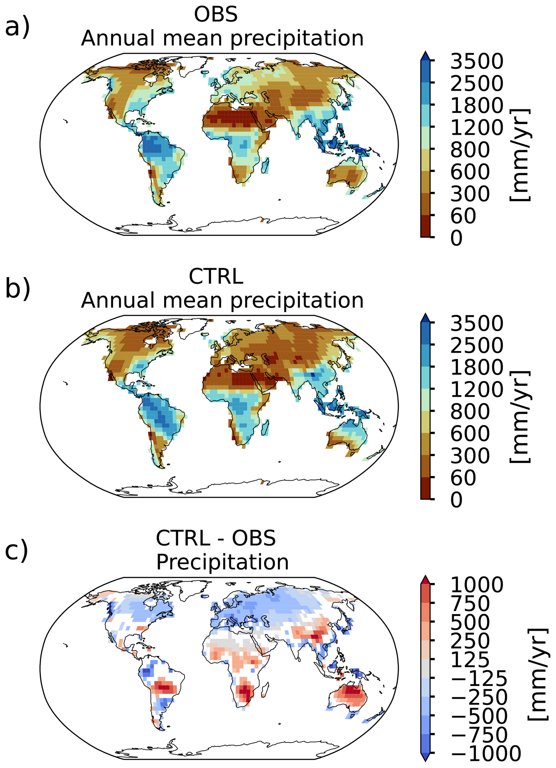
Figure A1 Comparison of ICON terrestrial climate in R2B3 configuration with the observation data (OBS). (a) The OBS annual mean precipitation (mm year⁻¹) averaged between 2000–2014 taken from the satellites estimate (Adler et al., 2018), (b) the CTRL simulation, (c) the difference between CTRL to OBS. Note that only land regions where the bias is greater than two standard deviations of the interannual variability of OBS precipitation are shown.

Appendix B: Additional tables

Table B1 Description of the corresponding functions for each organ.

(Farquhar et al., 1980)(Collatz et al., 1992)(Ryan, 1991)

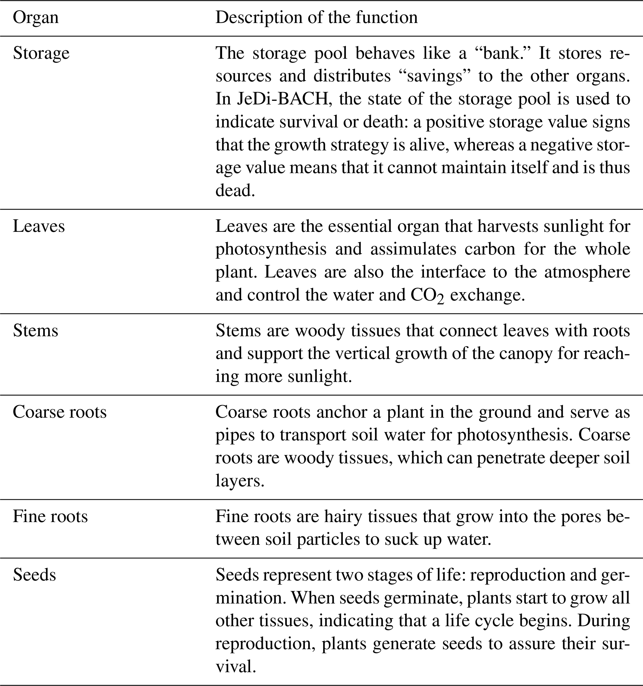
Table B2 Different components of JeDi-BACH and the corresponding original processes in JeDi-DGVM and JSBACH. A check-mark in the column “JeDi-DGVM” indicates that the respective process is newly implemented following the implementation of JeDi-DGVM and replaces a corresponding process description of JSBACH. Instead, a check-mark in the column “JSBACH” indicates that the process implementation of JSBACH is taken over into JeDi-BACH. P indicates that some parameters are modified for JeDi-BACH. M indicates that the processes are substantially modified for JeDi-BACH.

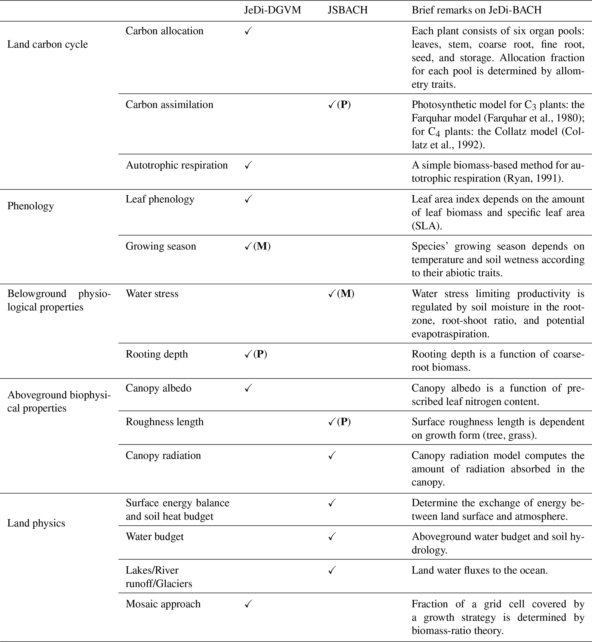
Table B3 Description of the 15 trait parameters. An illustration of each trait parameter is given as an example of a growth strategy with a large corresponding trait value compared to a species with a small trait value. C is short for carbon.

(Larcher, 1996)

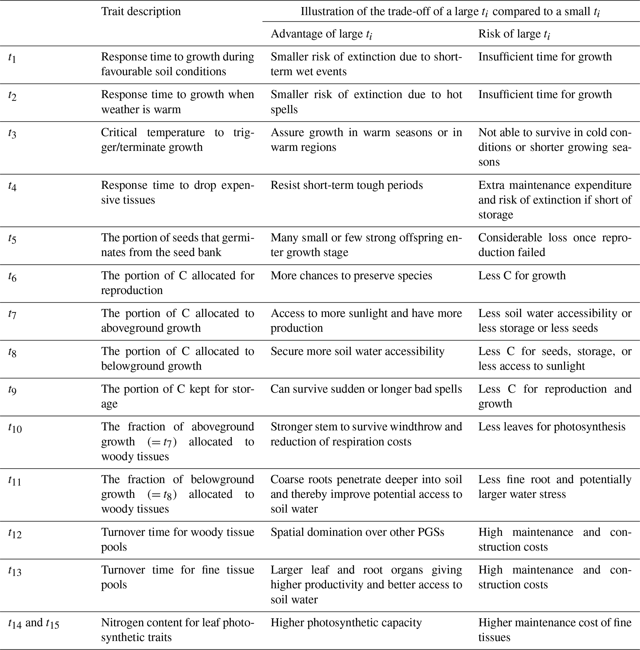
Table B4 Variables and parameters used in JeDi-BACH. Column 1 lists the symbols used in the model equations. Column 2 gives a brief description of the symbol and column 3 its units, in case of variables their range of possible values (if restricted), and for parameters their values used in the JeDi-BACH standard setup.

Appendix C: Remarks on modifications to the JeDi approach

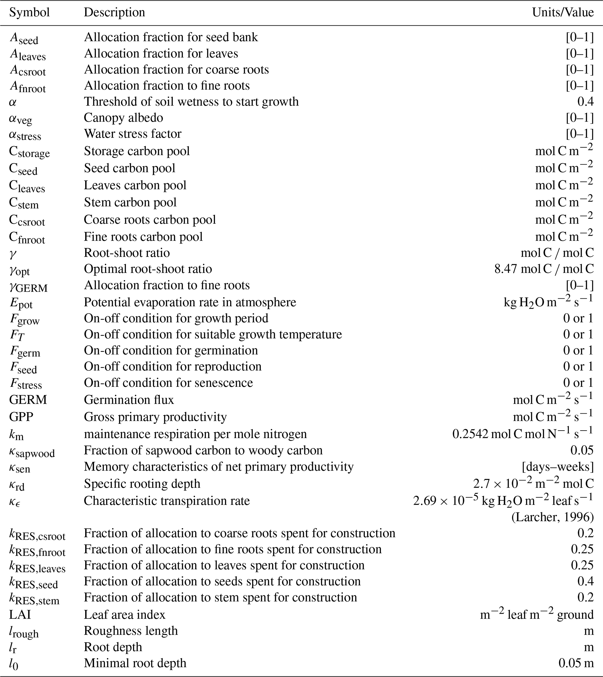
C1 Remarks on Sect. 2.4: Phenology

Concerning the modelling of phenology, JeDi-BACH deviates in two aspects from JeDi-DGVM (Pavlick et al., 2013). First, JeDi-BACH features a different set of rules to determine the ending of the growth period. In JeDi-DGVM, the same threshold temperature is used to bound the start and the end of a growth period – a choice that results in a relatively late termination of growth in mid to high latitudes. Thereby, plants continue to grow new tissues that are likely useless as productivity is reduced when days become shorter in late summer. This needlessly allocated carbon leads to less storage of carbon that plants photosynthesize in the summer/autumn to survive the winter and to regrow in spring. To remedy this, we introduced a separate threshold temperature to terminate the growth period in JeDi-BACH. This new threshold is combined with a new variable for detecting the warming/cooling trend (${\stackrel{\mathrm{‾}}{\mathrm{\Delta }T}}_{\mathrm{30}\mathrm{d}}$). With these two changes, growth ends when the weather becomes gradually colder, so that the growth period ends in those mid to high latitudes earlier than in JeDi-DGVM.

Second, enhanced senescence of non-woody tissues is made equal. As part of the original JeDi concept, strategies comprise a trait determining the relative difference in the enhancement of senescence between fine roots and leaves when they experience bad environmental conditions, detected by negative NPP. We removed this trait in JeDi-BACH so that senescence enhancement is equal for these organs, to the consequence that their senescence time scales are equal (even if not enhanced; see Eq. 21). This modification has been introduced to ensure that the relative carbon allocation to leaves and roots results in a fixed ratio between leaf and fine root carbon so that preferential allocation into leaves or fine roots are clearly different lifelong strategies. Therefore, strategies are born with a higher or lower lifelong risk of suffering from water stress (see Sect. 2.6 for more details).