ICON coupled to HAM-lite 1.0 in limited-area mode: an efficient framework for targeted kilometer-scale simulations with interactive aerosols

We present a new limited-area version of the aerosol–climate modeling system ICON coupled to HAM-lite. This new version is capable of simulating anthropogenic and natural aerosols and their climate effects in specific target regions. We demonstrate its flexibility and applicability through three case studies covering distinct aerosol regimes and processes: air pollution episodes in Central Europe, the emission and transport of sea salt aerosol in the Atlantic Arctic, and the simultaneous formation of smoke and desert dust plumes during the 2019–2020 Australian bushfire season. These case studies show the ability of the model to capture the regional-scale patterns and diurnal variability of the predominant aerosol types. They also indicate, however, systematic biases related to the simplified representation of aerosol emission, microphysics, and chemistry. The insights that we gained from these regional simulations will guide future developments of HAM-lite.

1 Introduction

Understanding atmospheric processes across scales remains a central challenge in climate science. Traditional Earth system models (ESMs) operate at horizontal resolutions of 𝒪(100 km) and need to parameterize key subgrid-scale phenomena such as gravity waves or deep convection, the dominant mechanics for the vertical distribution of radiative energy and the formation of tropical precipitation. New ESMs, also referred to as convection-permitting or storm-resolving, operate at horizontal resolutions of 𝒪(1 km) and have demonstrated significant improvements in the representation of the diurnal cycle, storm organization, and precipitation extremes (Prein et al., 2015; Schär et al., 2020). Global atmosphere-only simulations with grid spacings down to 2.5 km in the DYnamics of the Atmospheric general circulation Modeled On Non-hydrostatic Domains (DYAMOND) intercomparison confirmed that storm-resolving simulations are now possible, although still with a high computational effort (Stevens et al., 2019). The Next Generation of Earth Modeling Systems (nextGEMS) project has further shown that also decadal coupled simulations are now feasible (Segura et al., 2025).

Aerosols play a critical role in the Earth’s radiation budget and cloud microphysics, directly by absorbing and scattering solar and terrestrial radiation and indirectly by acting as cloud condensation or ice-nucleating particles (Boucher et al., 2013; Bellouin et al., 2020). The net effective radiative forcing of anthropogenic aerosols since 1750 is estimated to be about −0.3 W m⁻² $[-\mathrm{0.6},\mathrm{0.0}]$ W m⁻² for aerosol–radiation effects and −1.0 W m⁻² $[-\mathrm{1.7},-\mathrm{0.3}]$ W m⁻² for aerosol–cloud effects (Forster et al., 2021). The relatively large uncertainties of these estimates continue to be a challenge for climate projections. In most ESMs, aerosols are prescribed from climatologies or reanalyses rather than simulated interactively, limiting the ability to capture feedback mechanisms between aerosols, clouds, and atmospheric circulation. Furthermore, current ESMs with parameterized convection do not include explicit convective microphysics and therefore cannot represent the effects of aerosols on convective clouds (Prein et al., 2015; Stevens et al., 2019).

In recent years, the ICOsahedral Nonhydrostatic (ICON) ESM has been advanced to perform interactive regional to global simulations at kilometer and sub-kilometer resolution, far beyond the capabilities of previous state-of-the-art models (Giorgetta et al., 2018; Hohenegger et al., 2023). Recently, Segura et al. (2025) presented global coupled atmosphere–ocean simulations at resolutions of 5 to 10 km. Within this version of ICON, Weiss et al. (2025) developed the reduced-complexity aerosol module HAM-lite 1.0. HAM-lite is based on the well-established but more computationally demanding HAM module (Stier et al., 2005; Zhang et al., 2012; Tegen et al., 2019; Salzmann et al., 2022). Unlike HAM, which uses a full aerosol microphysical scheme, HAM-lite represents aerosols as an ensemble of log-normal modes with prescribed sizes and compositions. In that way, HAM-lite only requires one prognostic variable per mode, namely the aerosol number concentration. This significantly lowers computational costs while retaining the capability to explicitly represent aerosol–cloud interactions, including the effects of aerosols on convective clouds. The configuration of aerosol modes in HAM-lite is flexible. Here, we used the default configuration including two pure modes, one for dust and one for sea salt, and two internally mixed modes containing sulfuric and carbonaceous particles, respectively (Weiss et al., 2025).

Building on the work of Weiss et al. (2025), we developed a limited-area mode (LAM) version of the aerosol-climate model ICON coupled to HAM-lite 1.0, hereafter referred to as ICON-HAM-lite. This new version is designed for regional simulations at horizontal resolutions from 5 km to below 1 km. It supports targeted, computationally efficient simulations over specific source or receptor regions, making it particularly useful for aerosol process studies, regional climate research, and model development. It is complementary to sophisticated regional chemistry–transport models, such as ICON-ART (Schröter et al., 2018), COSMO-MUSCAT (Wolke et al., 2012), and WRF-Chem (Powers et al., 2017), by offering flexible aerosol mode configurations, substantially reduced computational costs and short run times suitable for extensive sensitivity experiments, ensemble studies, and configuration testing. At the same time, it maintains full consistency with the global ICON-HAM-lite framework, enabling seamless transitions between regional and global simulations.

We demonstrate the versatility of ICON-HAM-lite LAM through three cases that span diverse aerosol regimes and climates: (1) PM_2.5 air pollution episodes in Central Europe (March 2019), emphasizing the interplay of local emissions and long-range transport; (2) sea spray aerosol generation and transport in the Arctic Fram Strait (April 2020), highlighting marine source dynamics under marginal sea ice conditions; and (3) smoke and mineral dust emissions during the 2019–2020 Australian Black Summer bushfires (December 2019), where deep pyro-convective lofting and simultaneous transport of desert dust provide an interesting case of aerosol–radiation interactions. These examples show the capability of ICON-HAM-lite LAM to capture regional aerosol burdens, vertical distributions, and transport patterns in good agreement with observations.

In the following sections, we provide a brief overview of the aerosol module HAM-lite and a detailed description of the LAM version (Sect. 2). We then describe the different aerosol measurements used for model evaluation (Sect. 3). In Sect. 4, we compare the model simulations against in-situ and remote-sensing observations and present an initial analysis. Finally, we provide a summary of the current developments of HAM-lite and outline future directions for model improvements and further regional applications (Sect. 5).

2 Model description

The HAM-lite aerosol module is a one-moment scheme derived from the more comprehensive two-moment scheme HAM (Stier et al., 2005; Zhang et al., 2012; Tegen et al., 2019; Salzmann et al., 2022). It has been further developed and adapted in this study for simulations in limited-area mode. Its simplified structure enables efficient simulations of aerosol processes at high spatial resolution, now at both global and regional scales. A detailed model description, configuration guidance, and initial global test case has been presented by Weiss et al. (2025).

Table 1 Aerosol modes and properties used in the simulations of this study. Size ranges define the modal classification, while $\stackrel{\mathrm{‾}}{r}$ denotes the representative number-median radius of each log-normal mode. The values closely follow the configuration of Weiss et al. (2025), with matching volume fractions (α_k), densities (ρ), and hygroscopicities (κ); only minor differences exist in the modal radii. Volume fractions (α_k) are derived from AeroCom-II/ACCMIP (Heil et al., 2022), number-median radii ($\stackrel{\mathrm{‾}}{r}$) are adapted from MACv2 (Kinne, 2019), and species densities (ρ) and hygroscopicities (κ) are taken from ECHAM6.3-HAM2.3 (Tegen et al., 2019) and GISS-E2.1-MATRIX (Fanourgakis et al., 2019).

2.1 Aerosol microphysics and transport

In HAM-lite, aerosols are represented as an ensemble of internally mixed, log-normal modes with prescribed sizes and compositions (see Weiss et al., 2025). The size of a mode can fall within the nucleation, Aitken, accumulation, or coarse size range from below 0.005 µm to above 0.5 µm. And the composition of each mode can represent an arbitrary mixture of aerosol components. In this study, the default configuration includes mineral dust, sea salt, organic carbon, and black carbon, with all particles within a mode sharing the same composition (Riemer et al., 2019). Depending on the application, the relative volume fractions of these species can vary, ranging from a pure dust mode to predominantly carbonaceous mixtures with minor sulfate contributions. An example configuration of aerosol composition and modal properties used in this study is summarized in Table 1.

The size distribution of aerosols is given by J log-normal aerosol modes:

$$\begin{array}{}\text{(1)}& N\left(\ln r\right)=\sum _{j=\mathrm{1}}^J{\displaystyle \frac{N_j}{\sqrt{\mathrm{2}\mathit{\pi }}\ln {\mathit{\sigma }}_j}}\exp \left(-{\displaystyle \frac{(\ln r-\ln {\stackrel{\mathrm{‾}}{r}}_j{)}^{\mathrm{2}}}{\mathrm{2}{\ln }^{\mathrm{2}}{\mathit{\sigma }}_j}}\right),\end{array}$$

in which N_j is the number concentration, ${\stackrel{\mathrm{‾}}{r}}_j$ is the median radius, and σ_j is the geometric standard deviation of mode j (Seinfeld and Pandis, 2016).

In contrast to the HAM scheme, HAM-lite treats only the number concentrations as a prognostic variable, while the median radius (and composition) are prescribed. Consequently, particle properties, like density and hygroscopicity, can be precomputed as volume-weighted averages:

$$\begin{array}{}\text{(2)}& {\mathit{\rho }}_j=\sum _{k=\mathrm{1}}^K{\mathit{\alpha }}_{j,k}{\mathit{\rho }}_k,{\mathit{\kappa }}_j=\sum _{k=\mathrm{1}}^K{\mathit{\alpha }}_{j,k}{\mathit{\kappa }}_k,\end{array}$$

where K is the number of species, α_j,k is the volume fraction of species k in mode j, and ρ_k and κ_k are the density and hygroscopicity of species k. The wet radius and wet density are tabulated as a function of air temperature and relative humidity using growth factors from Petters and Kreidenweis (2007). The configuration of aerosol modes in HAM-lite is flexible and can be adapted to the research goals and available computational resources; additional components can be included by adding another mode. The optimal choice of prescribed aerosol properties may differ between global and regional configurations, depending on aerosol-specific transport, mixing, and aging characteristics across scales.

HAM-lite has been coupled to a new configuration of the ICON ESM designed for kilometer- and sub-kilometer-scale simulations, as described by Hohenegger et al. (2023). The aerosol modes of HAM-lite are added as prognostic tracers to the dynamical core of ICON, and the aerosol processes of HAM-lite are coupled with the atmospheric processes of ICON. The ICON model can operate in global and regional domains. In addition, it is possible to refine the resolution locally by adding nested domains, in which the nested domain feeds back to the outer domain via its boundaries.

To enable regional simulations with the ICON-HAM-lite model, we revised the handling of aerosol tracers as follows. First, we extended the tracer structures in HAM-lite by an additional dimension for the model domain or patch index, consistent with the existing ICON framework. Second, we integrated the aerosol tracers of HAM-lite into the reading routines for initial and lateral boundary conditions, allowing aerosol fields to be initialized and updated consistently with water tracers of ICON via the same data files. Third, we developed new preprocessing tools to extract the boundary conditions, anthropogenic emissions and surface properties from global, generic data sets. The boundary conditions for the aerosols can be taken from global HAM-lite simulations, the Copernicus Atmosphere Monitoring Service (CAMS; Inness et al., 2019), the MERRA-2 reanalysis from NASA (Gelaro et al., 2017), or even from idealized profiles.

2.2 Emissions

Emissions are either calculated online or prescribed according to emission inventories and associated scenarios. In the absence of explicit aerosol microphysics, emitted species are assigned directly to the prescribed modes, omitting intermediate transformation steps. These include secondary inorganic and organic aerosol formation via gas-to-particle conversion, as well as aging processes such as coagulation and condensation-driven particle growth. Their effects are nevertheless partly represented through the prescribed modal composition and size.

Anthropogenic emissions are based on commonly used inventories (e.g., Hoesly et al., 2018; Heil et al., 2022) typically reported as monthly means, while wildfire emissions are taken from satellite products (e.g., Kaiser et al., 2012) available as daily means. As newly implemented in this study, the sensible heat flux during wildfire events is incorporated using the satellite-derived fire radiative power (FRP), enabling grid cells with active fires to produce more realistic buoyancy-driven plumes of wildfire smoke. The specific emission inventories used in this study, as well as the FRP-based heat flux scaling, are described in detail in Section 2.5.1 “Model Configuration”. Sea salt emissions are calculated interactively following the parameterization by Gong (2003), which depends on surface wind speed and sea surface temperature. Similarly, dust emissions are calculated interactively using the scheme of Tegen et al. (2002), with modifications described by Cheng et al. (2008) and Heinold et al. (2016). The emissions are added to the aerosol modes of HAM-lite without any intermediate steps. To feed emissions into the modes, the mass fluxes from the emission datasets are converted into number fluxes. For mixed modes with multiple emission sources, the aerosol composition can be precomputed from the predefined emission fluxes as outlined in Weiss et al. (2025).

2.3 Removal processes

Aerosols are removed from the atmosphere by sedimentation as well as dry and wet deposition. The processes are briefly summarized here. More details can be found in the paper of Weiss et al. (2025). Gravitational sedimentation is computed throughout the vertical column using the wet particle radius. The settling velocity is based on Stokes’ law as described by Seinfeld and Pandis (2016), with non-continuum corrections following Riemer (2002). For numerical stability, the settling velocity is limited by the ratio of model layer thickness to time step. Sedimentation from the lowest model layer to the surface, which is driven by surface-dependent turbulent exchange, is treated in the dry deposition scheme.

The dry deposition flux is calculated as the product of number mixing ratio, air density, and dry deposition velocity. This velocity depends on aerodynamic and surface resistances, which vary with land surface types and are integrated over the fractional areas of different surface categories. The formulation follows the scheme of Pleim et al. (2022). The aerodynamic resistance is computed using the turbulence parameterization from ICON, which provides the friction velocity and similarity profile (Dipankar et al., 2015). The laminar sub-layer resistance incorporates empirical corrections that distinguish between vegetated and non-vegetated surfaces, with vegetation characteristics such as vegetation fraction and leaf area index provided by the land surface model JSBACH (Reick et al., 2021). Collection efficiencies due to Brownian diffusion and impaction depend on the Stokes and Schmidt numbers, with the latter incorporating a diffusion coefficient corrected for non-continuum effects following Riemer (2002). The Stokes number is formulated differently for vegetated and non-vegetated surfaces, using characteristic collector sizes specific to surface types such as coniferous and deciduous forests, grasslands, and water bodies. Similar to sedimentation, a numerical limiter is applied to the dry deposition velocity to ensure stability, based on the surface layer thickness and model time step. The resulting dry deposition flux is subtracted from the surface emission flux such that a net flux is passed to the turbulence scheme.

Wet deposition is implemented as a column-integrated process acting on cloudy model levels. A grid cell is considered cloudy when the cloud water and cloud ice mixing ratio exceed a threshold of 10⁻⁶ kg kg⁻¹ consistent with the criteria used in the cloud microphysics scheme (Baldauf et al., 2011). The wet deposition tendency combines three factors: (1) the number of aerosol particles activated at cloud base, which depends on the cloud base height and the local activation fraction; (2) the ratio of precipitating hydrometeors (rain, graupel, snow) to the total condensed water content (including cloud water and ice), representing the efficiency of precipitation formation; and (3) the ratio of surface precipitation to the column-integrated precipitating water content, representing the fraction of precipitation that reaches the surface. Together, these terms quantify the scavenging efficiency and removal of aerosols through in-cloud and below-cloud wet deposition processes.

2.4 Cloud microphysics and radiation interactions

The used ICON cloud microphysics is represented by the one-moment scheme of Baldauf et al. (2011), which computes the masses of water vapor and five hydrometeor types, including cloud water, cloud ice, rain, snow, and graupel. The number concentrations of cloud droplets and ice particles are not prognostic but are diagnosed based on aerosol and meteorological conditions. As described by Weiss et al. (2025), the aerosol module HAM-lite interacts with cloud microphysics via droplet activation and wet deposition processes. Cloud droplet activation is computed using the parameterization of Abdul-Razzak and Ghan (2000), which essentially depends on the updraft velocity and wet particle radius. The activated particles of all modes are added together to estimate the cloud droplet number concentration at cloud base, which is then assumed to remain vertically constant throughout the entire cloud column. Since a minimum cloud droplet number concentration of 30 cm⁻³ is imposed, similar to the threshold used by Goto et al. (2020). The diagnosed number concentration is used both in the autoconversion rate of cloud droplets within the microphysics scheme and in the calculation of cloud radiative properties within the radiation scheme (Seifert and Beheng, 2006; Pincus et al., 2019).

The radiative transfer in ICON is parameterized using the scheme by Pincus et al. (2019), which computes radiative fluxes across 14 shortwave and 16 longwave spectral bands. The aerosol tracers from HAM-lite are integrated into the radiative transfer calculations. Aerosol optical properties are derived at each vertical level using Mie theory following Stier et al. (2005, 2007). These properties are determined from look-up tables as functions of standard deviation, size parameter, and complex refractive index. The refractive index is computed as a volume-weighted average over all aerosol species, including water. The extinction coefficient, single scattering albedo, and asymmetry factor are computed per aerosol mode and combined to yield bulk optical properties. The extinction coefficient is computed for both longwave and shortwave radiation, whereas the single scattering albedo and the asymmetry factor are evaluated only for the shortwave bands (Bohren and Huffman, 1998; Siebesma et al., 2020). As dry size and composition in HAM-lite are prescribed, aerosol radiative properties are pre-calculated during the initialization stage of the model and tabulated as a function of relative humidity.

2.5 Simulation setup

To demonstrate the flexibility and applicability of the new regional version of ICON-HAM-lite, we perform three distinct case studies, each targeting a specific geographic region particularly relevant to one or more aerosol modes of HAM-lite. The regions are chosen to cover key aerosol regimes: (1) Central Europe for anthropogenic sulfate and carbonaceous aerosols, (2) Atlantic Arctic for sea salt aerosol, and (3) Southeast Australia for desert dust and wildfire aerosol. With these three studies, we aim to show the ability of ICON-HAM-lite to represent region-specific aerosol processes in distinct environments across the globe.

2.5.1 Model configuration

The aerosol setup in HAM-lite mirrors the configuration of Weiss et al. (2025), apart from minor adjustments in the modal radii. Mode radii are set slightly larger than in the reference configuration to represent more aged anthropogenic aerosol populations and to better capture sea-salt and desert-dust particle properties in and near their respective source regions. The aerosols are represented using four distinct modes, as summarized in Table 1. These include two pure modes, one for dust and one for sea salt, and two internally mixed modes containing organic carbon (OC), black carbon (BC), and sulfate. The carbon-dominated mixed mode represents aerosols from biomass burning and biogenic sources, including emissions from forest fires, grass fires, agricultural waste burning, and biogenic volatile organic compounds; hereafter, this mode is referred to as the carbonaceous mode. The sulfur-dominated mixed mode, hereafter referred to as the sulfuric mode, represents aerosols from volcanic sources and anthropogenic pollution, such as emissions from aviation, energy production and distribution, industry, maritime and land transport, waste treatment and disposal, as well as residential and commercial combustion. For studies with a more focused scientific objective, the composition and potentially also the size of the aerosol modes could be adjusted to better reflect regional characteristics.

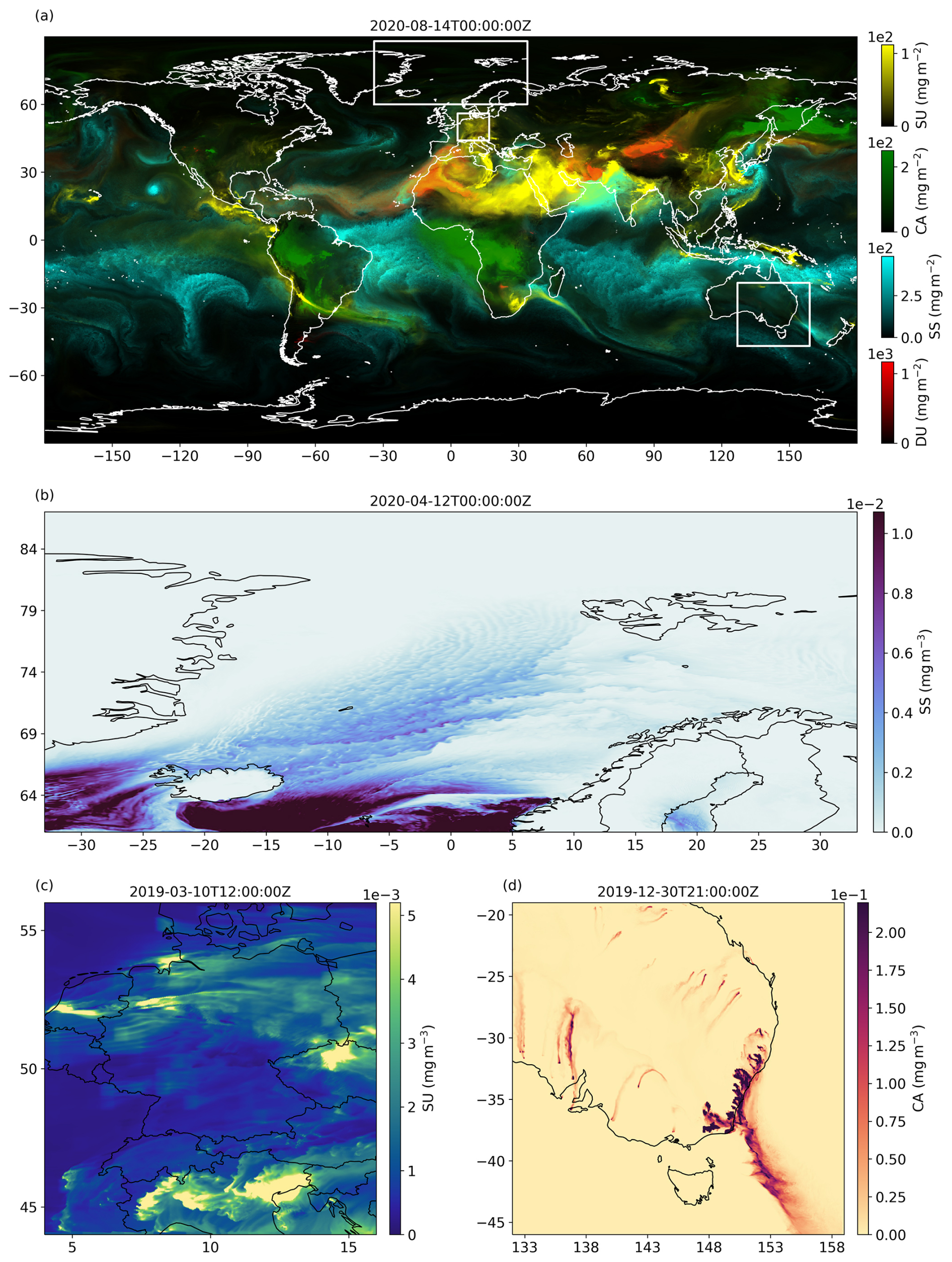
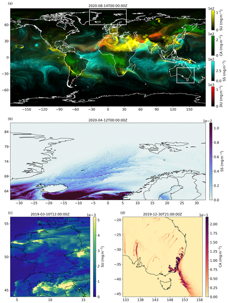
Figure 1 Scenes from a global simulation at a resolution of 5 km by Weiss et al. (2025) (a) and from the three regional simulations presented here at a resolution of 2.5 km (b–d). Panel (a) shows column burdens of dust (DU), sea salt aerosol (SS), carbonaceous aerosol (CA), and sulfuric aerosol (SU) as well as the boundaries of the three regional simulations. The panels below show snapshot surface concentrations for individual examples of (b) sea salt (SS) over the Arctic, (c) sulfuric aerosol (SU) over Germany, and (d) carbonaceous aerosol (CA) over Australia.

Table 2 Summary of the three LAM simulations presented in this study, including domain corners, modelled period, and grid information. Computing costs are given in node hours (NH) per simulated day (SD) (based on a 10 s model time step) on the DKRZ high-performance system Levante, whose compute nodes each contain AMD 7763 processors (128 cores in total) and 256 GB memory.

All simulations in this study are performed exclusively in limited-area mode with the ICON grid R2B10, which corresponds to a horizontal spacing of approximately 2.5 km. At a 2.5 km grid size, deep convection is largely resolved explicitly, while subgrid-scale processes such as cloud microphysics, turbulence, radiation, and aerosol processes, including activation and deposition, remain parameterized. In the vertical, a terrain-following hybrid sigma–z coordinate (Smooth LEvel VErtical coordinate, SLEVE) is used. The atmosphere is discretized into 90 levels with thicknesses ranging from 25 to 400 m, while the land surface is divided into five levels with thicknesses between 0.065 and 5700 m. For each case, a rectangular domain was defined, tailored to the spatial extent of the relevant aerosol phenomena. The Central Europe domain, with a focus on Germany, spans from approximately 44 to 56° N and from 3 to 17° E, covering the period of 1 to 11 March 2019. The Atlantic Arctic domain, centered around the Fram Strait and Svalbard and encompassing part of the Multidisciplinary drifting Observatory for the Study of Arctic Climate (MOSAiC; Shupe et al., 2021) expedition, extends from 60 to 88° N and from 34° W to 34° E, covering the period of 1 to 12 April 2020. The southeastern Australia model domain was selected to capture the combined impact of bushfire smoke and concurrent desert dust transport during the extreme fire event at the turn of 2019–2020. It extends from 19 to 47° S and from 127 to 159° E, and the simulation covers the period from 26 to 31 December 2019. Figure 1 shows scenes from a global simulation with ICON-HAM-lite (Fig. 1a), performed on the R2B09 grid with a horizontal spacing of approximately 5 km, along with the three regional domains presented in this study (Fig. 1b–d). The configuration of the three regional simulations is summarized in Table 2.

The anthropogenic emissions used are based on data from the Community Emissions Data System (CEDS; Hoesly et al., 2018; Feng et al., 2020; O'Rourke et al., 2021). This database provides monthly mean emissions from anthropogenic pollution sources at a spatial resolution of 0.1°, organized into different source sectors such as energy production, industrial combustion, transport, and domestic heating. Similar to Weiss et al. (2025), anthropogenic aerosol emissions are assigned to the internally mixed carbonaceous and sulfuric modes according to the prescribed modal composition, with only minor differences in the applied volume fractions provided in Table 1. The biogenic emissions are taken from the inventory of Guenther et al. (1995), which represents climatological biogenic emissions. As in the original HAM model (Stier et al., 2005; Zhang et al., 2012; Tegen et al., 2019), 15 % of biogenic monoterpene emissions are assumed to form secondary organic aerosol (SOA) directly at the surface, although it is acknowledged that SOA also forms aloft in reality. The biomass burning emissions, which contribute primarily to the carbonaceous aerosol mode, are prescribed using the daily values from the Global Fire Assimilation System (GFAS; Kaiser et al., 2012) at 0.1° resolution, which is based on fire radiative power (FRP) observations from the Moderate Resolution Imaging Spectroradiometer (MODIS) instruments aboard NASA's Terra and Aqua satellites. To represent the vertical injection of smoke, GFAS FRP is converted into an equivalent surface sensible heat flux (SHF) that is applied as a lower boundary forcing, similar to the approach of Muth et al. (2025). This conversion is implemented via a prescribed proportionality factor linking FRP to SHF. For the extreme Australian fires of 2019–2020, this proportionality factor was tuned such that the resulting SHF reached values of up to 8 kW m⁻², enabling the ICON-HAM-lite configuration to reproduce the observed pyro-convective injection of smoke (Kablick et al., 2020; Ohneiser et al., 2020), even though the limited resolution cannot capture fine-scale plume structures.

As described by Weiss et al. (2025), the physical properties of the aerosol species, such as densities and hygroscopicities, are taken from ECHAM6.3-HAM2.3 (Tegen et al., 2019) and GISS-E2.1-MATRIX (Fanourgakis et al., 2019). The number median dry radii are taken from the MACv2 aerosol climatology (Kinne, 2019), with adjustments to better match aerosol lifetimes reported by Gliß et al. (2021). The dry radii were mainly adjusted for the carbonaceous and sulfuric modes to correct for overestimated aerosol lifetimes under the initial assumptions.

2.5.2 Initial and boundary data

Atmospheric and land initial conditions, along with meteorological lateral boundaries, are obtained from analysis files produced by the Integrated Forecasting System (IFS; ECMWF, 2024) of the European Centre for Medium-Range Weather Forecasts (ECMWF), while ocean surface boundary conditions are taken from the AMIP II database (Taylor et al., 2000). All simulations are initialized with a clean atmosphere (i.e., without prior aerosol loading) and spun up for 1 to 2 d to allow for an initial adjustment of the aerosol fields. For the Central European and Atlantic Arctic case studies, aerosol lateral boundary conditions are taken from the Copernicus Atmosphere Monitoring Service (CAMS) reanalysis (Inness et al., 2019) to account for long-range aerosol transport. In contrast, no aerosol lateral boundary conditions are applied in the Australian case, since the dominant aerosol sources are located within the model domain and the focus is on local aerosol production. The CAMS reanalysis provides 6-hourly mass mixing ratios of organic carbon, black carbon, sulfate, mineral dust, and sea salt, which are converted to number concentrations and assigned to the corresponding aerosol modes of HAM-lite. For organic carbon, black carbon, and sulfate, which are represented as bulk species in CAMS, the respective median radii from HAM-lite are used for the conversion to number concentrations. For both dust and sea salt, the two smallest CAMS size bins are mapped to the corresponding HAM-lite modes. For sea salt, it is taken into account that the CAMS mass mixing ratios are reported at a relative humidity of 80 %. Following the CAMS documentation (Colette et al., 2025), the sea salt mass mixing ratios are therefore converted to dry mass by dividing by a factor of 4.3 before deriving number concentrations and assigning the particles to HAM-lite modes. The mapping is obtained by calculating the mass fraction of these CAMS bins that lies within the size range of the respective HAM-lite log-normal mode.

2.6 Computational performance

The LAM simulations with ICON-HAM-lite were carried out and analyzed on the Levante high-performance computing system at the Deutsches Klimarechenzentrum GmbH (2025). A total of 64 compute nodes were utilized, each equipped with 128 CPU cores and 256 GB working memory. The system requirements vary depending on the domain size. Therefore, to provide a basis for performance estimation, a computational unit (cu) is defined as 1 million grid cells × 1000 time steps. With a model time step of 10 s, this corresponds to 8.6 cu per simulated day for a domain with 1 million grid cells, and thus to 86 cu for a ten-day period. The values reported were averaged from 10 daily runs for each of the three case studies (see Table 2). For 1 cu, ICON-HAM-lite at R2B10 requires approximately 4 node hours. To put these performance metrics into context, the R2B10 LAM configuration in this study spans a range from about 2 cu for the German domain with roughly 0.2 million grid cells to about 14 cu for the Australian domain with roughly 1.6 million grid cells, with all cu values referring to the computational cost for one simulated day. This amounts to 8 node hours per simulated day for the German case and 56 node hours for the Australian case. In contrast, a global R2B10 simulation with roughly 84 million grid cells would require about 725 cu, corresponding to approximately 3000 node hours per simulated day. This illustrates the significant reduction in computational cost that can be achieved with the LAM version, provided the scientific focus can be limited to a regional domain.

3 Observational data for aerosol evaluation

3.1 Air quality monitoring

The ability of the model to reproduce particulate pollution over Central Europe, and Germany in particular, is evaluated by comparing the model results with ground-based observations from operational air quality monitoring networks. These observational datasets are provided by the European Environment Agency (EEA), which offers access through its download service (https://www.eea.europa.eu/en/datahub, last access: 15 June 2025) to time series of air composition at more than 5600 sites across Europe. The primary parameter analyzed in this study is fine particulate matter (PM_2.5), i.e., particles with an aerodynamic diameter of 2.5 µm or less. It is a key indicator for the assessment of air quality with regard to human health. The dataset contains hourly PM_2.5 concentration values from monitoring stations ranging from rural to urban sites, enabling spatiotemporal comparison with model simulations. This allows for a robust evaluation of the model's ability to represent observed air pollution levels and their time evolution under real-world conditions, including the four aerosol modes dust, sea salt, carbonaceous and sulfuric aerosol that together constitute PM_2.5 in HAM-lite. For comparison with the measurements, aerosol mass concentrations are calculated offline from the simulated number concentrations using the volume-mean radius and prescribed particle density of each log-normally distributed aerosol mode. Total aerosol mass is obtained by summing contributions from the four model aerosol modes, and a PM_2.5 size cut-off is applied.

3.2 Sea salt measurements

Modeled sea salt aerosol is evaluated by comparison with mass concentrations derived from in-situ chloride ion (Cl⁻) measurements collected by the European Monitoring and Evaluation Programme (EMEP) network. The data, which comprises various inorganic compounds in the gas and particle phase (e.g., ammonium, calcium, chloride, magnesium, sodium, and sulphate), can be obtained from the EBAS database (https://ebas.nilu.no, last access: 10 April 2025), maintained by the Norwegian Institute for Air Research (NILU). Sea salt mass concentrations are estimated from Cl⁻ using a conversion factor of 1.65, corresponding to its weight fraction in sea salt (Seinfeld and Pandis, 2016). Measurements from three high-latitude and coastal EMEP stations were used: Kårvatn (62.783° N, 8.883° E; 210.0 $\mathrm{m}\mathrm{a}.\mathrm{s}.\mathrm{l}.$) and Tustervatn (65.833° N, 13.917° E; 439.0 $\mathrm{m}\mathrm{a}.\mathrm{s}.\mathrm{l}.$) in Norway; as well as Irafoss in Iceland (64.083° N, 21.017° W; 66.0 $\mathrm{m}\mathrm{a}.\mathrm{s}.\mathrm{l}.$). These stations provide a reliable observational basis for evaluating the model over the North Atlantic region.

In addition to these stationary and permanent observations, in-situ aerosol measurements from the MOSAiC (Multidisciplinary drifting Observatory for the Study of Arctic Climate) drift experiment are used to evaluate modeled sea spray aerosol in the central Arctic. Conducted from October 2019 to July 2020 aboard the German research vessel (RV) Polarstern, MOSAiC offers a unique opportunity for a process-level evaluation of Arctic aerosol throughout the full Arctic year (Frickenhaus et al., 2022). Among other measurements, a comprehensive set of in-situ observations was collected that includes the bulk size-resolved chemical composition and mass concentration of non-refractory sub-micron aerosol particles (e.g., sulfate, nitrate, ammonium, chloride, and organics) (see Heutte et al., 2023a, b for further details on measurement procedures and data processing).

3.3 Space-based lidar observations

Lidar observations from the Cloud–Aerosol Lidar with Orthogonal Polarization (CALIOP; Winker et al., 2013) instrument aboard NASA’s Cloud–Aerosol Lidar and Infrared Pathfinder Satellite Observations (CALIPSO) satellite are used to retrieve vertical profiles of the extinction coefficient at 532 nm. In this study, the level-2 version 4 aerosol profile product (05kmAPro), averaged over 5 km horizontal segments along the near-nadir ground track, is used to evaluate the atmospheric layering and plume heights of the modeled dust and bushfire aerosol in the Australian case. Although CALIOP often fails to detect thin aerosol layers in the upper troposphere and lower stratosphere (e.g., Watson-Parris et al., 2019), the significant aerosol enhancements resulting from the Australian wildfires are clearly captured. These extinction profiles, despite sampling and detection biases in individual profiles, provide valuable constraints for model evaluation. The modeled extinction coefficients are calculated offline from the number mixing ratios using a mass-specific extinction coefficient of 0.5 and 1.0 m² g⁻¹ for desert dust and carbonaceous aerosol, respectively (Ansmann et al., 2012; Reid et al., 2005; Laskin et al., 2015), with particle properties summarized in Table 1.

4 Results and discussion

Here, we analyze the simulations outlined in Sect. 2 to demonstrate the potential and flexibility of the new limited-area configuration of ICON-HAM-lite. Rather than providing a comprehensive evaluation, we focus on showing its capabilities through the three distinct case studies, which span diverse aerosol regimes and processes, highlighting the broad range of applications supported by this model.

4.1 PM_2.5 pollution over Germany

PM_2.5 is a core target parameter for both health risk assessments and air quality regulations, but also plays a complex and significant role in the Earth’s climate. Dominant sources in Germany are primary emissions from road traffic, industry, domestic heating, agriculture, and construction. In addition, long-range transport and secondary aerosol formation can contribute substantially to PM_2.5 concentrations, particularly during springtime pollution episodes. Consequently, air quality in Germany can be strongly influenced by emissions from neighboring countries and meteorological conditions, which can trap pollutants or enhance long-range transport impacts (e.g., Renner and Wolke, 2010; Pültz et al., 2023). In 2019, all German air quality monitoring stations complied with the EU annual mean limit for PM_2.5 of 25 µg m⁻³, continuing the trend of steadily decreasing concentrations since the threshold was implemented in 2015. However, more than half of the nearly 200 stations (57 %) still exceeded the WHO’s stricter annual recommendation of 10 µg m⁻³, and almost all stations (98 %) recorded more than three daily exceedances of 25 µg m⁻³, thus failing the WHO’s 24 h guideline (UBA, 2020).

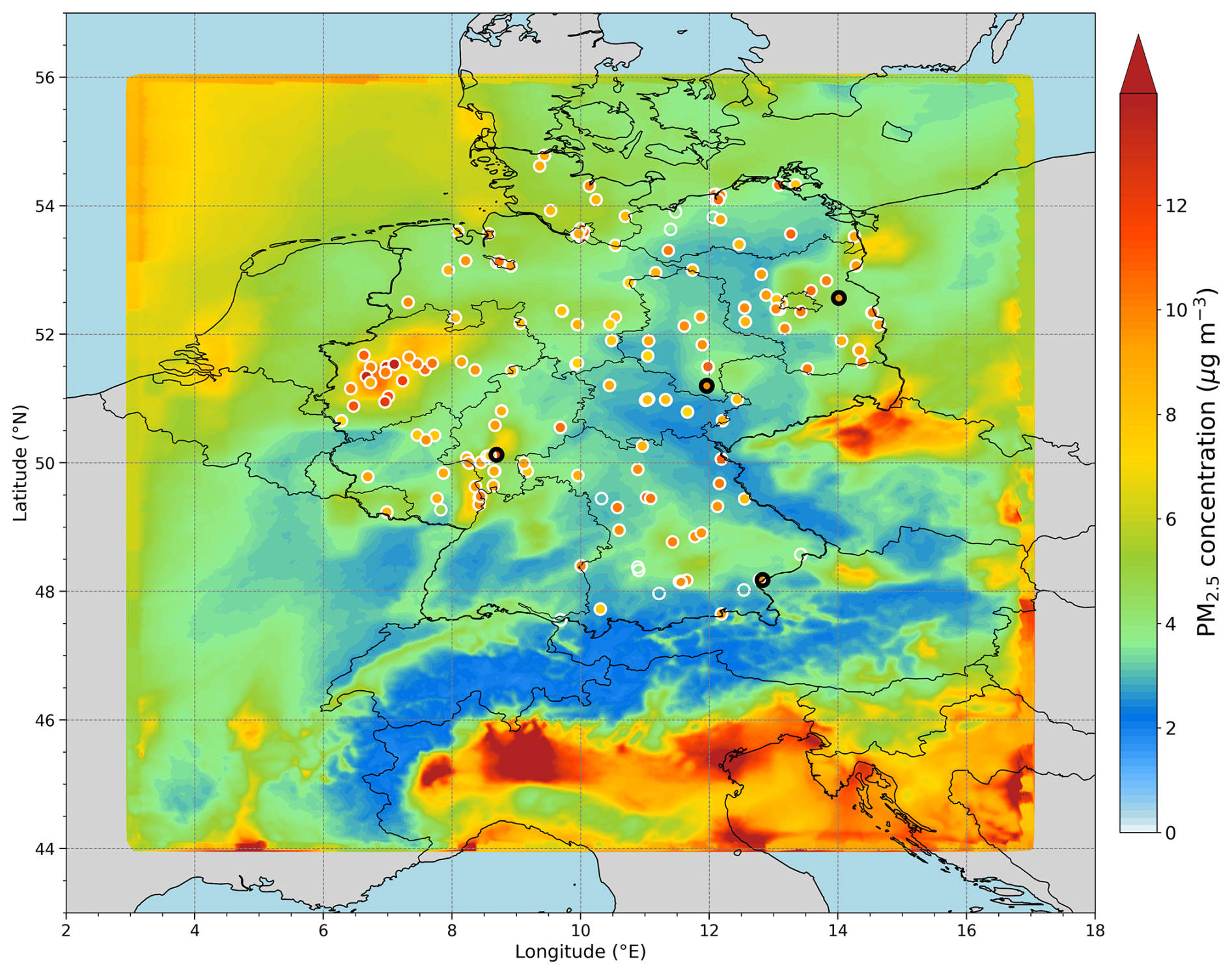
Figure 2 PM_2.5 surface concentrations averaged over 3 to 11 March 2019 including contributions from carbonaceous aerosol (CA), sulfuric aerosol (SU), mineral dust (DU), and sea salt (SS) as computed by ICON-HAM-lite. Observations from the EEA air quality monitoring network are overlaid as circles, with black markers indicating the stations included in the time-series analysis in Fig. 3.

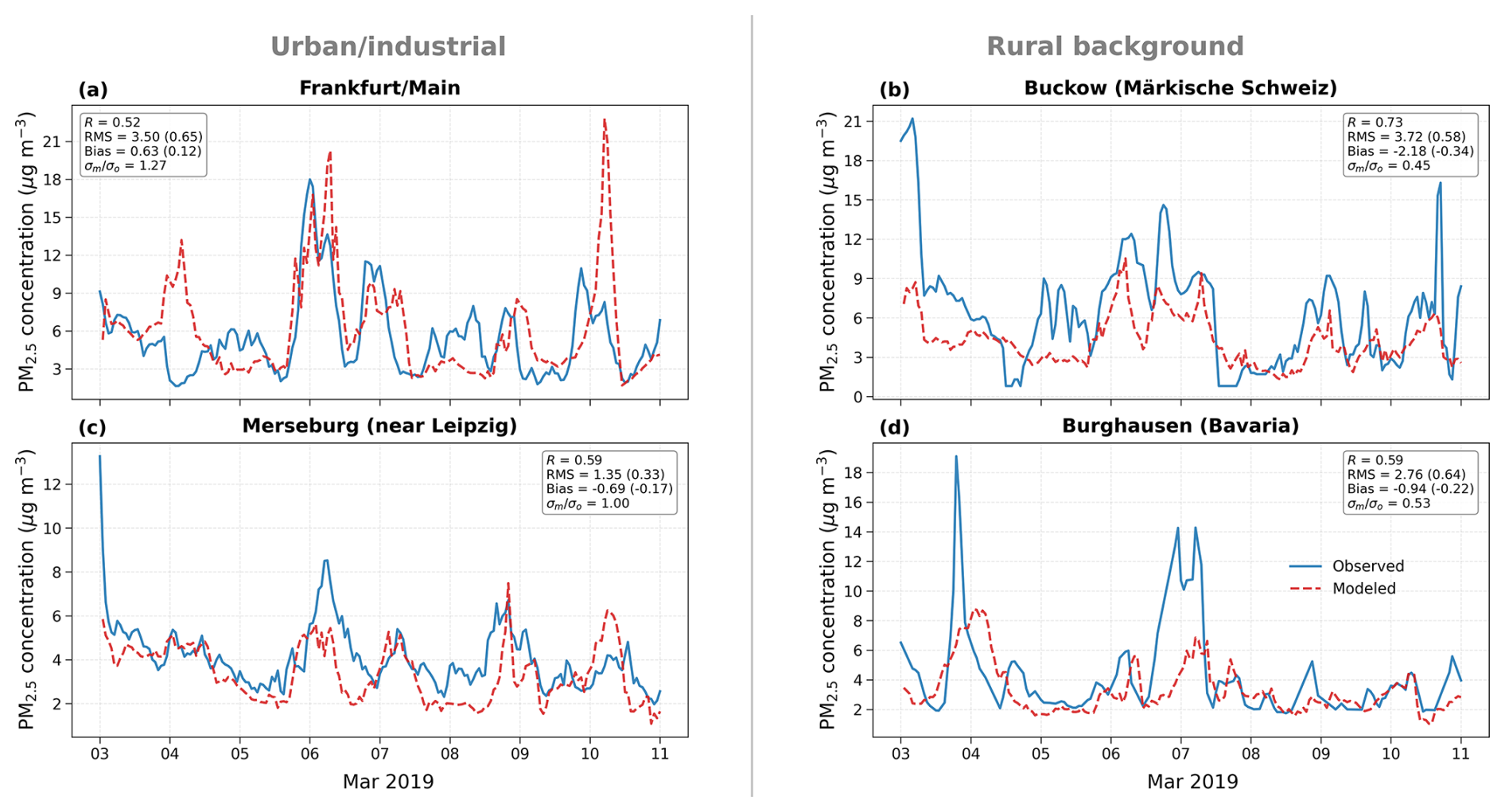
Figure 3 Hourly time series of observed and modeled PM_2.5 surface concentrations at the urban/industrial sites (a) Frankfurt/Main and (c) Merseburg near Leipzig as well as the rural background sites (b) Buckow in the Märkische Schweiz and (d) Burghausen in Bavaria from 3 to 11 March 2019 (See the map in Fig. 2 for their geographic locations.). The observations are from the EEA air quality monitoring network. The model data are taken from ICON-HAM-lite simulations and include mass contributions from carbonaceous aerosol, sulfate, dust, and sea salt. For each panel the correlation coefficient R, the root mean square error RMS (normalized RMS in parenthesis), the absolute bias (normalized bias), and the ratio between simulated and observed standard deviation (${\mathit{\sigma }}_{\mathrm{m}}/{\mathit{\sigma }}_{\mathrm{o}}$) are given.

Figure 2 shows the spatial distribution of modeled mean PM_2.5 concentrations over Central Europe for the period from 3 to 10 March 2019, as simulated by the ICON-HAM-lite model. In HAM-lite, PM_2.5 represents the total mass concentration of four aerosol modes: dust, sea salt, carbonaceous, and sulfuric. For the comparison to measurements, the modal number concentrations are integrated over their size distributions and truncated at a 2.5 µm diameter cutoff. Observations from the European Environmental Agency (EEA) air quality monitoring network for Germany are superimposed on the map as circles. The modeled PM_2.5 concentrations exhibit pronounced regional gradients. Low concentrations below 4.0 µg m⁻³ dominate rural and mountainous areas such as central, southern, and northeastern Germany, the Alps, and eastern France. High concentrations up to 25.0 µg m⁻³ occur in densely populated and industrialized regions – especially northwestern Germany, i.e. Ruhr region, Rhine–Main region, the Bohemian basin in Czech Republic, southwestern Poland, and the Po Valley in northern Italy. These hot-spots align with sources of high anthropogenic emissions and regions with limited atmospheric ventilation. The model captures the major regional features and concentration gradients reasonably well. However, it tends to underestimate PM_2.5 levels in central remote areas and in an eastern range from the Thuringian Forest to the Bavarian Forest, as well as in the Black Forest region in the southwest, likely due to the absence of processes forming secondary inorganic and organic aerosols. Secondary inorganic aerosol components such as ammonium and nitrate, which can contribute substantially to PM_2.5 during pollution episodes and long-range transport events, are not explicitly represented in the present HAM-lite configuration. Conversely, peak concentrations are frequently overestimated in urban and industrial regions, possibly due to simplified assumptions in the time profiles of the prescribed anthropogenic emissions.

To further examine the spatial context, time series of PM_2.5 concentrations are shown for two urban/industrial sites (Frankfurt am Main and Merseburg near Leipzig) and two rural background sites (Buckow in Märkische Schweiz and Burghausen in Bavaria) in Fig. 3. These plots compare hourly modeled values with observed concentrations over the same period. In the observations, rural sites show average concentrations around 6.5 µg m⁻³ (Buckow) and 4.4 µg m⁻³ (Burghausen), with peak concentrations reaching up to 21.2 µg m⁻³ (Fig. 3b an d). While mean PM_2.5 levels at urban and rural sites partly overlap, urban locations show enhanced temporal variability and more pronounced short-term pollution episodes. The average urban concentrations lie at 5.5 µg m⁻³ (Frankfurt) and 4.1 µg m⁻³ (Merseburg), and the peak concentrations are up to 18.0 and 13.3 µg m⁻³, respectively (Fig. 3a and c). The model reproduces the timing of concentration peaks relatively well in urban areas but consistently overestimates their magnitude. In rural areas, modeled values show better agreement in magnitude but tend to underestimate short-term peaks, suggesting missing processes related to secondary aerosol formation or long-range transport.

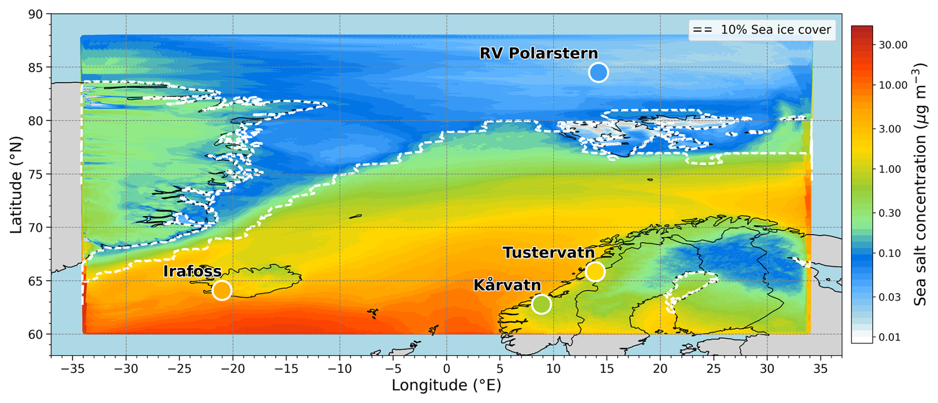
Figure 4 Surface concentration of sea salt over the Atlantic Arctic averaged over 4 to 12 April 2020 as computed by ICON-HAM-lite. Circles indicate observations from EMEP sites and the RV Polarstern during the MOSAiC expedition. The dashed white line marks the sea ice edge, defined as the boundary where sea ice concentration reaches 10 %.

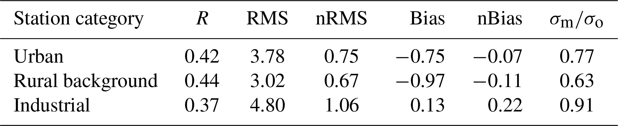
This is consistent with quantitative evaluation metrics shown in Fig. 3, which indicate moderate agreement between simulations and observations, with correlation coefficients of 0.52–0.73 and normalized RMS errors of 0.33–0.65 across the four stations. A broader statistical evaluation across all German stations is summarized in Table 3. Rural background stations show the lowest normalized RMS errors (0.67), while industrial stations exhibit the largest errors (1.06). Correlation coefficients remain moderate and relatively similar across all station categories (R = 0.37–0.44). The larger errors at industrial sites are consistent with the model tendency to overestimate short-term pollution peaks in regions with strong anthropogenic emissions, whereas the lower variability at rural background stations likely reflects missing secondary aerosol formation and long-range transport contributions.

Table 3 Mean statistical evaluation metrics for modeled versus observed PM_2.5 concentrations at German station categories shown in Fig. 2. Urban stations include traffic, industrial, and urban background sites, while background stations comprise rural and rural-regional background sites. Shown are the correlation coefficient (R), the absolute and normalized root mean square error (RMS, nRMS), the absolute and normalized bias (Bias, nBias), and the ratio between simulated and observed standard deviation (${\mathit{\sigma }}_{\mathrm{m}}/{\mathit{\sigma }}_{\mathrm{o}}$).

Together, the spatial and temporal comparisons demonstrate the model’s skill in capturing regional-scale patterns and diurnal variability of PM_2.5, while also indicating systematic biases related to the representation of emission sources and the simplification of aerosol microphysics and chemistry.

4.2 Sea salt aerosol in the Atlantic Arctic

Sea spray aerosol, which originates from open ocean water and leads and consists mainly of sea salt, is a significant but highly variable source of atmospheric particles in the Atlantic Arctic, especially during the melt season and summer months (Leck and Bigg et al., 2005; Lawler et al., 2021). When reaching a certain size, the sea spray particles can act as nuclei in cloud formation processes that influence the surface energy budget by scattering and absorbing incoming and outgoing radiation. The MOSAiC 2019–2020 expedition covered extended periods in the Atlantic sector of the Arctic Ocean. The German research vessel (RV) Polarstern drifted through the Fram Strait/Svalbard region during late summer and early autumn 2020 and provided observations relevant to the production of sea spray in open waters and marginal ice zones (Boyer et al., 2023).

Figure 4 shows the spatial distribution of surface concentrations of sea salt aerosol averaged from 4 to 12 April 2020 over the Atlantic Arctic region. The map covers the area between Greenland and Svalbard, a region strongly influenced by marine boundary layer dynamics. Observational data from European Monitoring and Evaluation Programme (EMEP) stations and the MOSAiC drift campaign aboard the RV Polarstern are overlaid as circular markers for comparison. The modeled sea salt concentrations range from below 0.03 µg m⁻³ in the inner Arctic to more than 30 µg m⁻³ over the Greenland Sea and coastal North Atlantic. Elevated concentrations are most prominent in regions of active sea spray generation, particularly in the vicinity of Iceland and along the Norwegian Sea coast. The simulation captures fine-scale emission structures, such as enhanced concentrations along the east coast of Greenland linked to Piteraq wind events, and along the sea ice edge west of Svalbard associated with cold-air outbreaks.

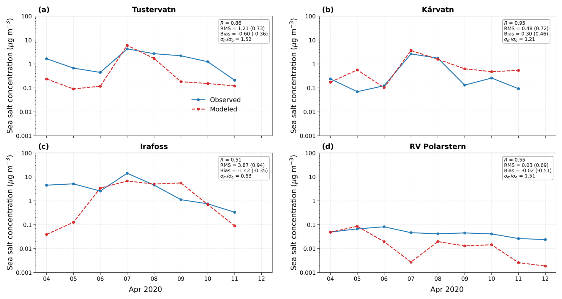
Figure 5 Daily mean sea salt concentrations at the EMEP stations (a) Tustervatn, (b) Kårvatn and (c) Irafoss, as well as on board RV Polarstern from 4 to 12 April 2020 (The location of the three stations and RV Polarstern are shown in Fig. 4). Observations are shown in blue and modeled values in red. For each panel the correlation coefficient R, the root mean square error RMS (normalized RMS in parenthesis), the absolute bias (normalized bias), and the ratio between simulated and observed standard deviation (${\mathit{\sigma }}_{\mathrm{m}}/{\mathit{\sigma }}_{\mathrm{o}}$) are given.

The comparison in the map is supported by the time series in Fig. 5, which show daily mean sea salt concentrations at the three EMEP stations and on board RV Polarstern. These time series provide additional context for the point measurements overlaid in Fig. 4, showing the day-to-day variability relative to the temporal mean in the map. At Tustervatn (Fig. 5a), observed concentrations vary between about 0.5 and 4 µg m⁻³, with a pronounced peak around 4 µg m⁻³ on 7 April. The model captures both the timing and magnitude of this event reasonably well, although the peak concentration is somewhat overestimated. Kårvatn (Fig. 5b) exhibits observed concentrations between about 0.07 and 2.0 µg m⁻³ with a peak just above 2 µg m⁻³. The model reproduces the temporal evolution of the sea salt episode very well, including the timing and magnitude of the main peak, while slightly overestimating concentrations during the later part of the period. At Irafoss (Fig. 5c), observed concentrations span roughly 0.3–12.0 µg m⁻³, with a pronounced maximum around 7 April. The model captures the occurrence of this event but underestimates the peak concentration and does not fully reproduce the subsequent decline. Along the RV Polarstern drift (Fig. 5d), observed concentrations remain relatively low, below 0.1 µg m⁻³. The model reproduces the low-concentration background conditions and some of the observed variability, although concentrations are generally underestimated during the second half of the period.

Quantitative evaluation metrics shown in Fig. 5 indicate strong temporal agreement at the Scandinavian stations, with correlation coefficients of 0.86 and 0.95 at Tustervatn and Kårvatn, respectively, while agreement is more moderate at Irafoss and along the RV Polarstern drift (R = 0.51 and 0.55). Normalized RMS errors remain below unity at all stations (0.69–0.94), indicating generally good agreement between simulated and observed concentrations. The remaining discrepancies are primarily related to the magnitude of individual peak events and the representation of low background concentrations.

The comparison with the available measurements shows that ICON–HAM-lite successfully reproduces the key spatial patterns and temporal variability of sea salt aerosol concentrations in this climatically important region, although biases in concentration magnitude remain.

4.3 Australian bushfire smoke and desert dust

The austral summer of 2019–2020, known as Australia’s Black Summer, saw unprecedented wildfires in southeastern Australia, burning nearly twice the area of any previous record (Boer et al., 2020). The activity of wildfires peaked around 29 December to 4 January, during which time deep pyro-convective towers lofted smoke aerosols up to 14–16 km into the lower stratosphere (Kablick et al., 2020; Ohneiser et al., 2020). According to Peterson et al. (2021), a remarkable amount of 0.3–1.1 Tg of smoke was injected in these 4 d, which was then rapidly advected eastward across the southern mid- and high latitudes. At the same time, intense dust emissions occurred in the interior of the continent, triggered by frontal passages and moist convection (see Fig. 6 in Peterson et al., 2021 for a synoptic overview), with mineral dust likewise lofted and transported eastwards. The coexistence of dust and bushfire aerosol makes this case particularly interesting for studying vertical transport processes and aerosol–radiation interactions.

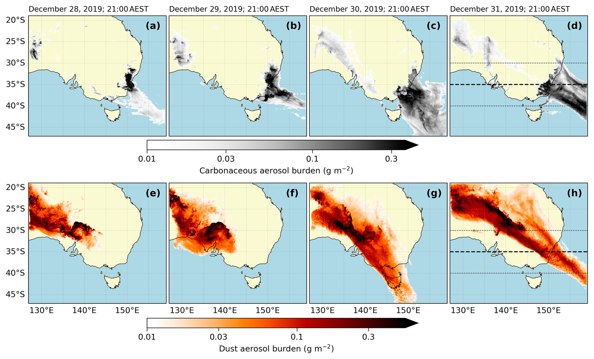
Figure 6 Maps of column burden of (a–d) carbonaceous aerosol and (e–h) dust aerosol over southeastern Australia and the southwestern Pacific Ocean on 28–31 December 2019, as computed with ICON-HAM-lite. The dashed line in panels (d) and (h) marks the center of the zonal cross-section shown in Fig. 7, while the dotted lines indicate the 10°-wide latitude band used for averaging.

Figure 6 shows column burdens of desert dust and carbonaceous aerosols over southeastern Australia from 28 to 31 December 2019. The maps illustrate the intense plumes of desert dust and bushfire smoke over southeastern Australia and adjacent oceanic regions. The simulations include the effect of fire radiative heat release on surface temperature, which induces strong buoyant updrafts and enables pyro-convective lofting of smoke emissions from the surface into higher atmospheric layers, in some cases up to the lower stratosphere. Fire radiative power (FRP) from NASA's MODIS observations, as provided by the GFASv1.2 dataset, is used to represent the spatial and temporal variability of fire activity and the corresponding intensifications of the sensible heat flux on the ground.

The smoke is lofted rapidly and dispersed over long distances, with prominent eastward advection over the Tasman Sea and into the South Pacific. Figure 6a–d, shows the wide spread of carbonaceous aerosol, which is consistent with satellite observations during this period (cf. Peterson et al., 2021; Nguyen et al., 2021). In regions with intense bushfire activity, carbonaceous aerosol burden can locally exceed 15.0 g m⁻², while values within the broader fire plume reach up to 0.3 g m⁻². Desert dust, mainly originating from central Australia, is also advected southeastward, interacting with the smoke plumes and contributing to the complex aerosol mixture. Maximum dust burdens of locally 7 g m⁻² are reached in the source areas and up to 0.3 mg m⁻² along the transport path (Fig. 6e–h).

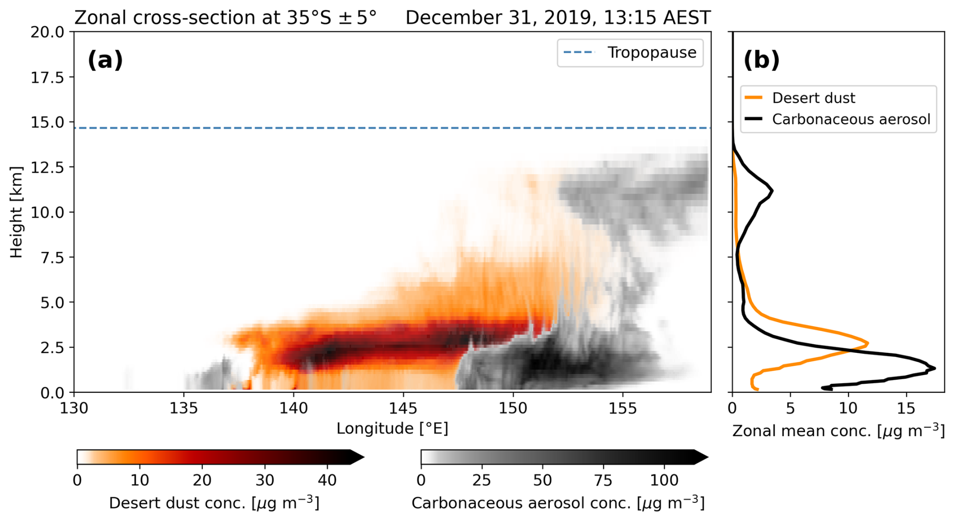
Figure 7 Panel (a) shows the zonal cross-section of aerosol concentrations averaged over the 5°-wide latitude band 35° ± 5° latitude on 31 December 2019, showing the vertical and longitudinal distribution of desert dust (colored shading) and carbonaceous aerosol from bushfires (grayscale). The horizontal dashed line denotes the approximate tropopause height. Panel (b) shows corresponding zonal mean vertical profiles.

To illustrate the vertical distribution and long-range transport of aerosols in more detail, Fig. 7a shows a zonal cross-section of aerosol concentrations averaged over a 10°-wide latitude band centered at 35° S on 31 December 2019. The figure distinguishes between desert dust (colored shading) and carbonaceous aerosol (grayscale shading), originating primarily from the intense bushfire activity in southeastern Australia. Figure 7b shows the corresponding zonal mean vertical profiles.

Carbonaceous aerosols are clearly dominant, with near-surface concentrations reaching up to about 110.0 µg m⁻³ in proximity to the wildfire source regions. Elevated smoke layers are also evident above 10 km and extend toward the modeled tropopause at approximately 14 km (indicated by the dashed blue line). These high-altitude plumes are consistent with pyro-convective events that loft smoke and associated aerosol particles into the upper troposphere and lower stratosphere. This vertical transport mechanism plays a key role in extending the atmospheric lifetime of carbonaceous aerosols and enhancing their radiative impact, as particles at these altitudes are subject to reduced removal processes (Peterson et al., 2018; Khaykin et al., 2020; Mueller et al., 2025).

In contrast, desert dust shows a more localized and lower-altitude distribution. Dust concentrations reach more than 40 µg m⁻³ but are largely confined to the lower troposphere, typically below 6 km. This reflects the difference in emission sources and injection mechanisms between the two aerosol types: while dust is lifted by mechanical processes such as turbulent winds and frontal activity, wildfire smoke is buoyantly injected through intense thermal updrafts known as pyro-convection. Nevertheless, a fraction of dust is also lofted to the transport heights of the smoke in this case.

The zonal mean profiles in Fig. 7b highlight these differences. The carbonaceous aerosol profile shows a broad, bimodal shape with peaks near the surface and at upper tropospheric levels, whereas the dust profile peaks at an altitude of about 2.5 km. These vertical gradients have implications for both short- and longwave radiative forcing in this region and throughout the Southern Hemisphere (Heinold et al., 2022; Senf et al. , 2023). While further analysis is beyond the scope of this study, the ICON-HAM-lite LAM model is ideally suited to investigate these effects in future work. In particular, the impacts of the pyro-convective parameterization through the FRP-scaled surface sensible heat flux, as well as the role of complex aerosol–radiative interactions in shaping the observed aerosol layering, will be analyzed in detail in a follow-up study.

To evaluate the aerosol layering, Fig. 8 shows extinction coefficient profiles at 532 nm from ICON-HAM-lite together with observations from the CALIOP instrument aboard NASA's CALIPSO satellite. Two CALIPSO overpasses from 31 December 2019 at 03:21 and 14:04 UTC that intersect the model domain are selected as shown in the inset map of Fig. 8. For each track, the profile with the maximum extinction above 5 km altitude is identified to focus on the evaluation of aerosols in the upper troposphere and lower stratosphere (UTLS). This profile is then averaged with adjacent profiles within a 5 km radius along the track to reduce noise and better represent the regional vertical structure.

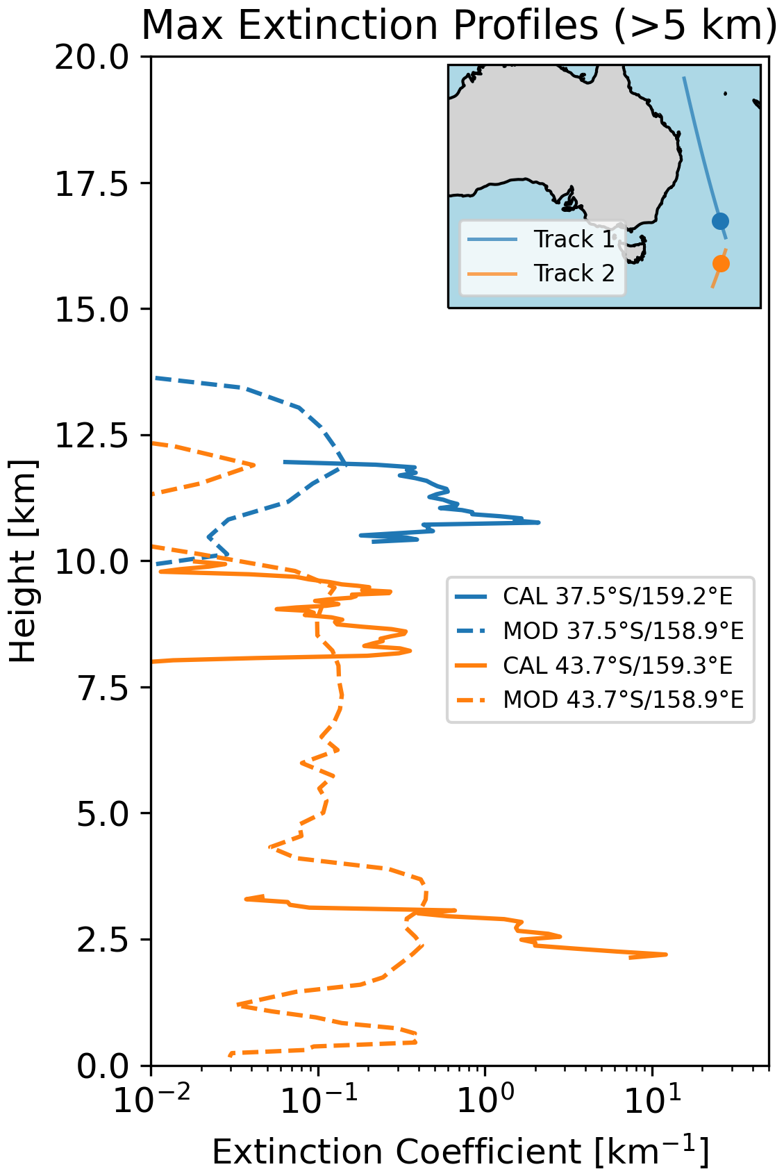
Figure 8 Comparison of vertical profiles of the aerosol extinction coefficient at 532 nm from CALIOP (solid lines) and ICON-HAM-lite (dashed lines) for two CALIPSO tracks over Southeast Australia on 31 December 2019. The CALIOP profiles are averages of the maximum extinction profile above 5 km and adjacent profiles within a 5 km radius along the track, to highlight upper-layer aerosol and reduce noise. The CALIPSO tracks are shown in the inset map, with filled circles marking the positions of the maximum profiles. Track 1 (blue) corresponds to the overpass at 03:21 UTC, and track 2 (orange) corresponds to the overpass at 14:04 UTC.

The profile from the northern CALIPSO track, i.e. track 1 in the inset of Fig. 8, shows elevated aerosol extinction between approximately 10–12.5 km altitude, with a peak near 11 km reaching values of up to  2 km⁻¹. This suggests lofted smoke layers near the upper troposphere, likely due to pyro-convection, as discussed above. The model reproduces the plume height well but shows somewhat higher extinction values and slightly broader vertical structure. In the southern track, i.e. track 2 in the inset of Fig. 8, CALIOP shows a pronounced extinction maximum of about 12 km⁻¹ at 2.5 km altitude, along with additional extinction signals above 8 km. This indicates the presence of both boundary-layer smoke and lofted aerosols, including desert dust. Again, the model captures the vertical extent reasonably well but likely underestimates the magnitude of the extinction coefficient. While the modeled profiles show reasonable agreement with observed vertical layering, CALIOP profiles are notably more fragmented. This likely reflects known limitations in CALIOP's ability to detect thin aerosol layers in the upper troposphere and lower stratosphere and to distinguish between aerosol and cloud features (e.g., Watson-Parris et al., 2019). Nevertheless, the agreement in plume height provides confidence in the model representation of smoke injection and transport processes.

Overall, these results underscore again the importance of accurately representing aerosol vertical distribution in atmospheric models, particularly for extreme biomass burning events with injection heights, which can reach stratospheric levels (Heinold et al., 2022). The ICON-HAM-lite LAM version offers a considerable advantage in this context, as it enables explicit calculation of pyro-convective injection instead of relying on uncertain parameterizations. Furthermore, it allows systematic experiments with different sources of uncertainty, which would be prohibitively expensive in a global model configuration.

5 Conclusions and outlook

In this study, we have introduced and evaluated a new limited-area version of the aerosol–climate model system consisting of ICON coupled to HAM-lite. By improving the treatment of aerosol tracers in the model and using pre-processing tools for initial and lateral boundary conditions, ICON-HAM-lite is now capable of interactive aerosol simulations over user-defined regions with minimal computational effort. Three illustrative case studies – Central European PM_2.5 pollution (March 2019), Arctic Fram Strait sea spray production (April 2020), and the 2019–2020 Australian bushfire event – demonstrate that the model can realistically reproduce regional aerosol burdens, vertical distributions, and transport patterns. The results were obtained with a fraction of the computational time required for more complex regional aerosol–chemistry–transport models, albeit with a deliberately reduced emphasis on detailed aerosol microphysical and chemical processes, in order to prioritize the explicit representation of key physical processes related to cloud formation and aerosol–cloud interactions, particularly those associated with convection. Processes like moist convection, gravity waves, and topographic disturbances are therefore captured explicitly.

The simulation for Central Europe reproduced major PM_2.5 hot-spots and diurnal variability, albeit with systematic biases in peak magnitudes linked to simplified secondary aerosol formation. It should be noted that while we largely used the aerosol configuration from the global simulation by Weiss et al. (2025), the compositions and sizes of the aerosol modes could be adjusted in future science-oriented studies, further improving the agreement with observed regional conditions. In the Atlantic Arctic, the model successfully resolved small-scale sea salt emission patterns and summertime concentration gradients in good agreement with EMEP and MOSAiC observations. For the Australian bushfire event, the deep pyro-convective lofting and long-range transport of smoke aerosol could be represented well by including scaled FRP-driven sensible heat fluxes. The simultaneous transport of desert dust in this case adds to the complexity of aerosol layering and potential radiative interactions (not investigated here).

These results confirm that the limited-area version provides a flexible, cost-effective framework for process-level aerosol studies in regions of interest, especially for natural primary aerosols. However, the model is not designed to compete with comprehensive regional air-quality systems in terms of chemical or aerosol microphysical complexity, but to address a different set of scientific questions. By operating at convection-permitting resolution, the limited-area version resolves clouds and convective dynamics explicitly and enables a consistent coupling of aerosols to cloud microphysics without the use of convection parameterization. Due to its physical consistency with the global ICON-HAM-lite configuration, the limited-area setup directly complements the existing global model version, enabling efficient sensitivity experiments and ensemble simulations over selected regions while retaining the option to apply the same configuration at global scale. At grid spacings on the order of 1 km, this approach supports physically coherent simulations of aerosol transport in convection-resolving environments and provides a robust foundation for advancing regional aerosol modeling toward explicitly resolved aerosol–cloud interactions that remain beyond the reach of global models and full chemistry–transport systems at comparable resolution, at least to date.

Looking ahead, several avenues of development can further enhance the utility of the limited-area (and global) version of ICON-HAM-lite. For example, the inclusion of an additional prognostic aerosol mode, e.g., for nitrate or secondary organic aerosol, would improve fidelity in pollution-dominated regimes. In addition, leveraging the low computational costs, one could perform a large ensemble of perturbation experiments targeting emission uncertainties, sensitivities to boundary conditions, and process parameterizations. Furthermore, targeted comparisons with simulations using sophisticated aerosol–chemistry–transport models over identical domains can be used to identify strengths and limitations of the simplifications and assumptions in HAM-lite. The high resolution of the model simulations aligns with the spatial scales of various in situ and remote sensing observations, such as imagery from ESA’s new EarthCARE (Earth Clouds, Aerosols and Radiation Explorer; Wehr et al., 2023) satellite, which improves both the model evaluation and the interpretation of the observational data (Schutgens et al., 2016). Scientifically, follow-up studies will particularly exploit the online coupling of aerosol, radiation, and clouds in the model to quantify region-specific aerosol–cloud–radiation interactions under convective and mixed-phase conditions. Future case studies may include wildfire smoke–dust mixtures in regions such as West Africa, as well as low-level mixed-phase clouds in the polar regions of Arctic and Antarctic.

In summary, the limited-area version of ICON-HAM-lite achieves a pragmatic balance between computational efficiency and physical representativeness, opening new opportunities for focused regional aerosol–climate research and rapid hypothesis testing. By making interactive aerosol simulations possible at kilometer scales, this framework will contribute to improve our understanding of aerosol processes and will enable the effective design of observational campaigns.