DeepMIP-Eocene-p2: Experimental design for Phase 2 of the early Eocene component of the CMIP7/PMIP7 Deep-time Model Intercomparison Project (DeepMIP-Eocene)

Warm, high-CO₂ climates of Earth's past provide an opportunity to evaluate climate models under extreme forcing, and to explore mechanisms that lead to such warmth. One such time period is the early Eocene (∼56–41 million years ago), when global mean surface temperatures were ∼15 °C higher than preindustrial, and CO₂ concentrations were ∼1500 ppmv. In this paper we present the experimental design for Phase 2 of the Eocene component of the Deep-time Model Intercomparison project (DeepMIP-Eocene-p2). The aim is to provide a framework for modelling groups to carry out a common set of simulations, thereby facilitating exploration of inter-model dependencies. The focus is on the early Eocene Climatic Optimum (EECO, ∼53.3–49.1 million years ago). Relative to Phase 1 of DeepMIP-Eocene, we provide a new paleogeography (topography, bathymetry) derived from several recent independent reconstructions that focused on different regions, a new vegetation distribution derived by merging paleobotanical data with vegetation model simulations, and a new CO₂ specification derived from recent re-evaluations of proxy data. The core set of simulations consists of a preindustrial control, an abrupt increase to 4× preindustrial CO₂ concentration from this preindustrial control, a standard control EECO simulation at 5× preindustrial CO₂ concentration, and an EECO simulation with preindustrial CO₂ concentration. In addition to these core simulations, we suggest a suite of optional sensitivity studies, which allow the impact of various factors to be explored, such as topography/bathymetry, greenhouse gases, land-surface parameters, astronomical and solar forcings, and internal model parameters. The updated boundary conditions and guidance on initialisation and spinup in Phase 2 will allow more robust model-data comparisons, more accurate insights into mechanisms influencing early Eocene climate, and increased relevance for informing future climate change projections.

1 Introduction

The study of paleoclimates, and in particular the study of paleoclimates using climate models, generally has two main motivations. First, to study the past climate of our Earth from a purely “blue-skies” curiosity-driven desire to better understand the planet that we live on, in particular the forcings and mechanisms/feedbacks that determine past climate change – because, as George Mallory reportedly said in regard to climbing Mount Everest, “it is there” (Rak, 2021). Second, to leverage information from Earth's past climates in order to better understand and predict future climates, so to inform political decisions regarding climate-related policy and to enable society to better adapt to future climate change. The Deep-time Modelling Intercomparison Project (DeepMIP) is driven by these two motivations, and is dedicated to conceiving, designing, carrying out, analysing, and disseminating, an international effort to improve our understanding of deep-time climates. “Deep-time” is here defined as any time period older than the Pliocene period, i.e. older than 5.3 million years ago. The objectives of DeepMIP are:

• to foster closer links between the palaeoclimate modelling and data communities,

• to design experiments for the MIP, through discussion with both model and data communities,

• to carry out such simulations with a wide range of models,

• to create, collate, and synthesise datasets where appropriate to enable meaningful model-data comparisons,

• to analyse the results with the aims of evaluating the models, understanding the reasons behind the model-model and model-data differences, and, where possible, providing suggestions for model improvements; and

• to carry out the above in such a way as to facilitate contribution to the Intergovernmental Panel on Climate Change (IPCC).

DeepMIP is a part of the Paleoclimate Modelling Intercomparison Project (PMIP), which itself is a part of the Coupled Model Intercomparison Project (CMIP), which is a project of the World Climate Research Program (WCRP). Together with the Pliocene Model Intercomparision Project (PlioMIP) effort (Haywood et al., 2024), DeepMIP-Eocene (Lunt et al., 2021) and DeepMIP-Miocene (Burls et al., 2021) extend PMIP efforts back beyond the Quaternary, to sample the full range of paleoclimate states that are comparable, at least in terms of CO₂ concentration, with the projected Shared Socioeconomic Pathways (SSPs; Meinshausen et al., 2020).

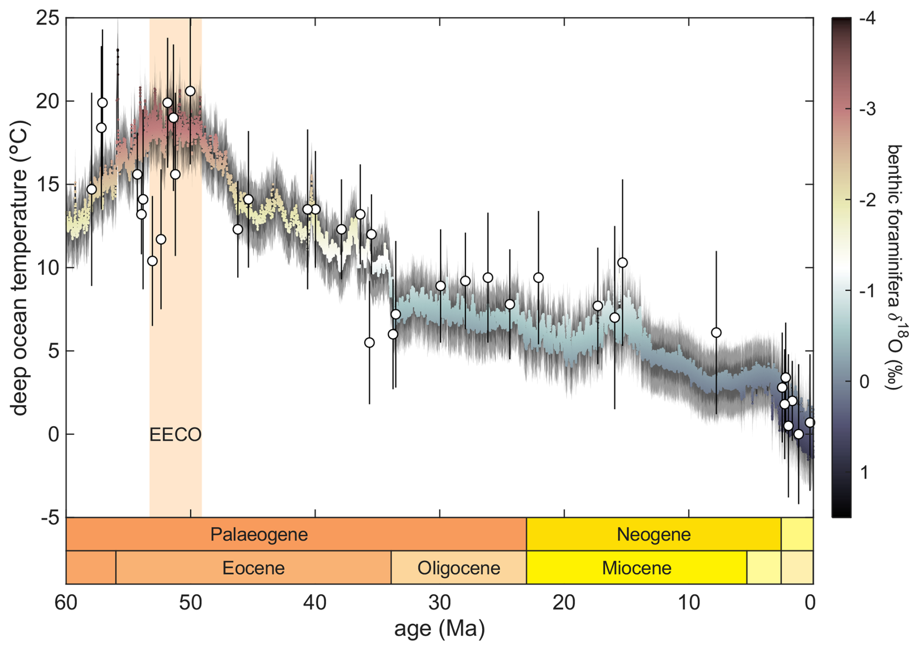
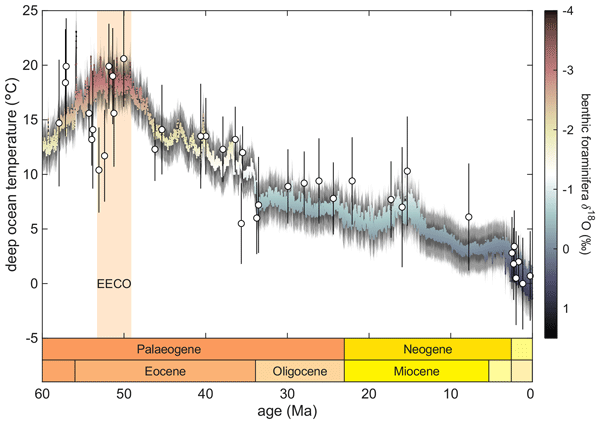
Figure 1 Deep ocean temperature through the Cenozoic, derived from: (i) the composite benthic foraminifera δ¹⁸O record (Westerhold et al., 2020), converted to temperature following Evans et al. (2024) including a pH correction; coloured line, and (ii) the clumped isotopic composition of benthic foraminifera (Meckler et al., 2022), using the calibration of Meinicke et al. (2020) and updated to the I-CDES scale (Meinicke et al., 2021); white circles. The early Eocene Climatic Optimum (EECO; ∼53.3–49.1 million years ago as defined by Hollis et al., 2019) is highlighted, which is the focus of DeepMIP-Eocene Phase 2. The colour scale of the δ¹⁸O-derived deep ocean temperature record transitions from red to blue at the approximate value associated with the Eocene–Oligocene Transition, marking the onset of major Antarctic ice growth.

Here, in preparation for CMIP7/PMIP7 (Dunne et al., 2025), we focus on the Eocene component of DeepMIP: DeepMIP-Eocene. The Eocene (56.0 to 33.9 million years ago), is a geological epoch that is characterised by a substantially warmer climate than modern (Fig. 1). Within the Eocene, much previous focus in DeepMIP has been on the early Eocene Climatic Optimum (EECO); ∼53.3–49.1 million years ago (Hollis et al., 2019). Proxies indicate global mean near-surface temperatures about 10–17 °C higher than preindustrial (Inglis et al., 2020a; Evans et al., 2024), CO₂ concentrations of ∼1500 ppmv (Anagnostou et al., 2020, see also Sect. 2.2.1), and no ice sheets. Proxies also indicate wetter high latitudes than modern (Cramwinckel et al., 2023; West et al., 2020), and a vegetation consistent with a generally warmer and wetter climate than modern, including a poleward expansion of temperate and warm-temperate forests in regions today covered by tundra shrub and boreal forests (Thompson et al., 2025). In the context of the Phanerozoic (last 540 million years), the paleogeography at this time was relatively similar to today, with distinct Atlantic, Indian, and Pacific oceans, and with the modern continents recognisable in terms of their relative positioning (see Fig. 3). However, the paleogeography differed from the modern in several respects, including an open Panama Seaway, constricted Tasman seaway and Drake passage, an open Tethys seaway, India disconnected from southeast Asia, and changes to the heights and configurations of multiple mountain ranges (Herold et al., 2014, and references therein). Despite these differences in paleogeography, the climate of the early Eocene has been compared to possible future climates under very high emissions scenarios (Burke et al., 2018; Arias et al., 2021), and has been used to constrain Equilibrium Climate Sensitivity (ECS, e.g. Forster et al., 2021; Inglis et al., 2020a). As such, the EECO provides a window to a substantially warmer world than today. It provides an opportunity to evaluate models, to use models to inform the interpretation of proxy records, and to provide mechanistic understanding of climate feedbacks in a warm world.

The first phase of DeepMIP-Eocene was based around a model experimental design in which paleogeography, CO₂, and vegetation boundary conditions were prescribed (Lunt et al., 2017), informed to a large extent by the work of Herold et al. (2014). Eight modelling groups submitted simulations to the first phase, the results from which are available in the DeepMIP model dataset (Steinig et al., 2024) and have been discussed in multiple studies, which are summarised very briefly here. Lunt et al. (2021) presented an overview of the large-scale temperatures, partitioning the modelled global mean surface temperature (GMST) and temperature gradients to different mechanisms through an energy-balance analysis, finding that a subset of the models showed results that were consistent with the proxies in terms of GMST, temperature gradient, and CO₂, and finding that non-CO₂ boundary conditions contributed between 3–5 °C to Eocene warmth. Kelemen et al. (2023) found that these non-CO₂ boundary conditions also played a key role in the meridional heat transport, leading to more heat transported to the South Pole by the ocean, and more heat transported northwards in the northern mid-latitudes by transient atmospheric eddies. Goudsmit-Harzevoort et al. (2023) found a strong 1–1 coupling between deep ocean and surface air temperature change across the ensemble, and found a best fit with deep ocean temperature proxies at 6× preindustrial CO₂ concentration. Evans et al. (2024) supported this finding, indicating that changes in deep ocean temperatures in general correlate well with changes in surface temperature. Cramwinckel et al. (2023) explored the large-scale modelled hydrology, finding a thermodynamically-dominated hydrological response leading to wettening in the mid and high latitudes, drier conditions in the subtropics, and wettening in the deep tropics, and finding that those models with the weakest meridional temperature gradients were in best agreement with precipitation proxies. Regional precipitation patterns and model-data comparisons were explored in Africa by Williams et al. (2022) and in Australia by Reichgelt et al. (2022). Both these studies estimated the CO₂ concentration for which the model simulations best agreed with the proxy vegetation data; Reichgelt et al. (2022) found best agreement at 6×, in contrast to Williams et al. (2022) who found best agreement at much lower values (as low as 1×); this apparent discrepancy is yet to be explored in detail. Abhik et al. (2024) showed that the modelled early Eocene Asian wet season was weaker than present day in the ensemble, and attributed this to the reduced Tibetan Plateau, and that this dominated over the response to the CO₂ forcing. Furthermore, by carrying out additional paleogeographic sensitivity studies, Zhang et al. (2022b) showed that the East Asian precipitation was determined to a large extent by the Southeast Mountains. Meijer et al. (2024) showed that proxies indicate monsoonal precipitation in the Asian continental interior during the early Eocene, but that this is not reproduced to such an extent in the DeepMIP-Eocene model results. Zhang et al. (2022a) found that all the models were dominated by strong deepwater formation in the Southern Ocean, at locations determined by Southern Ocean gateway geometry, but that one model also showed strong deepwater formation in the North Pacific, and that two models also showed deepwater formation in the North Atlantic. In the Pacific, there was a northward migration of the subtropical gyre, as evidenced in DeepMIP-Eocene models and the sedimentary record (Zhang et al., 2025). The lack of direct evidence of sea ice in the Eocene, coupled with the presence of subtropical taxa (e.g. Willard et al., 2019) and extensive temperature forest (e.g. West et al., 2020) in the Eocene Arctic, means that model simulations with extensive EECO sea ice are problematic to reconcile with the proxy record. In this context, Niezgodzki et al. (2022) investigated modelled sea ice during the Eocene, finding that the CO₂ threshold for formation of Arctic ice was very model dependent, and that implementation of river run-off and ocean basin connections were important for determining these model differences.

Although these studies arising from Phase 1 of DeepMIP-Eocene have considerably advanced our understanding of Eocene climate, there are some aspects of the experimental design which mean that uncertainties remain. For example, the paleogeography and vegetation boundary conditions which were prescribed in the Phase 1 model simulations have been superseded by more recent reconstructions (see Sect. 2.2.2), and the standard CO₂ concentration of 840 ppmv is low compared with recent proxy reconstructions (see Sect. 2.2.1). Also, the recommended initial condition for the ocean temperature had an unrealistic vertical profile, and as a result several models may have been relatively far from full equilibrium by the end of their simulations, which could potentially add additional model-model discrepancies. In addition, models themselves have improved since Phase 1, and computing power has increased, meaning that more advanced models could be used. It is therefore timely to define a new set of recommended boundary conditions to allow a Phase 2 of DeepMIP-Eocene.

In this paper we describe boundary conditions and experimental protocols for DeepMIP-Eocene Phase 2 (DeepMIP-Eocene-p2). Section 2.1 describes the choice of time period and core simulations, Sect. 2.2 describes the boundary conditions, Sect. 2.3 includes suggestions for sensitivity studies, Sect. 2.4 describes the initialisation and stabilisation protocols, and Sect. 2.5 describes the format for model outputs. The paper concludes with a summary (Sect. 3).

2 Experimental design

2.1 Choice of time periods, overview of experimental design, and simulation list

In the experimental design for DeepMIP-Eocene Phase 1 (Lunt et al., 2017), three periods within the Paleocene/Eocene were explicitly identified for study – the Paleocene-Eocene Thermal Maximum (PETM), the latest Paleocene or pre-PETM, and the EECO. These corresponded to the same three periods for which data compilations were presented in Hollis et al. (2019) and Inglis et al. (2020a), which were defined as representing 56, 57–56, and 53.3–49.1 Ma, respectively. However, model simulations for these periods differed solely in their prescribed CO₂ concentration, and the paleogeography used was originally designed to be most appropriate for 55 Ma. Subsequent analyses of model results, and model-data comparisons, tended to focus on the EECO. In Phase 2 we decide to continue this focus on the EECO, 53.3–49.1 Ma.

The paleogeography and vegetation boundary conditions for Phase 2 have been updated from Phase 1, as described in detail in Sect. 2.2.2 and 2.2.3 respectively, and we provide the appropriate boundary conditions as NetCDF files on Zenodo (Lunt, 2025b).

The CO₂ boundary condition is discussed in more detail in Sect. 2.2.1; in summary, we follow Phase 1 in suggesting sensitivity simulations at multiple CO₂ concentrations (see Sect. 2.3), but increase the “standard” CO₂ from 3× preindustrial CO₂ concentration (henceforth 3×PI) to 5× preindustrial CO₂ concentration (henceforth 5×PI), to be more in line with recent CO₂ proxies.

Thompson et al. (2025)Herold et al. (2014)

Table 1 Summary of simulations associated with DeepMIP-Eocene Phase 2, including two mandatory relevant simulations from CMIP7 (piControl and abrupt-4xCO2), the mandatory two standard simulations (deepmip-eocene-p2-5xCO2 and deepmip-eocene-p2-1xCO2), and some of the suggested sensitivity studies. Mandatory simulations are in bold.

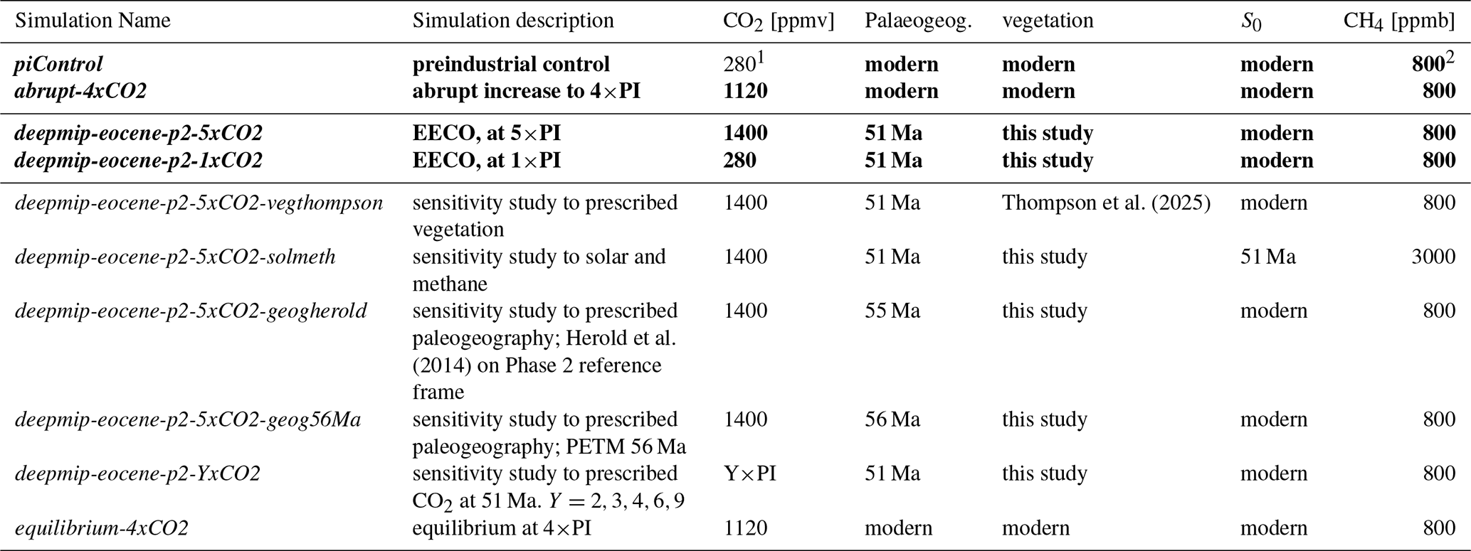
¹ If a value different from 280 ppmv is used for piControl, then all other CO₂ values in the table should be changed accordingly, as a ratio. Note that Meinshausen et al. (2017) suggests 284.3 ppmv for CMIP6 piControl simulations. ² If a value different from 800 ppbv is used for piControl, then all other CH₄ values in the table should be changed accordingly, as a ratio. Note that Meinshausen et al. (2017) suggests 808.2 ppbv for CMIP6 piControl simulations.

The primary EECO boundary conditions described in Sect. 2.2 define the standard DeepMIP-Eocene Phase 2 simulation (deepmip-eocene-p2-5xCO2, Table 1). In addition, the analysis of the DeepMIP-Eocene Phase 1 ensemble benefitted greatly from the existence of a preindustrial control (simulation piControl, Table 1) and an Eocene simulation at 1×PI (simulation deepmip-eocene-p2-1xCO2, Table 1), which allowed anomalies relative to preindustrial and the contribution of non-CO₂ forcings to be readily identified. As such, we retain these simulations in Phase 2, and make the 1×PI Eocene simulation mandatory.

Assessment of the relevance of the simulations for constraining ECS, for example through emergent constraints, was hampered by the absence of an instantaneous modern 4×PI simulation for many models. As such, we make this simulation mandatory in Phase 2 (abrupt-4xCO2, Table 1), allowing the ECS of every model to be calculated robustly and consistently across the model ensemble. The standard length of this ECS-determining simulation is relatively short at 150 years, and will likely already exist for some models as it is a core simulation in the “DECK” of CMIP7 (Dunne et al., 2025), and as such it should not represent a substantial computational burden. Some models may use different internal model parameters in their standard modern and Eocene configurations (e.g. differences in background vertical diffusivity). In this case, it should be clearly documented which version of the model the abrupt-4xCO2 simulation, and the associated preindustrial control, are carried out with (or, ideally, both versions should be used).

Other aspects to be explored in sensitivity studies, depending on the resources available, include paleogeography, vegetation, and the prescribed solar luminosity and methane (see Sect. 2.3).

A list of all the mandatory simulations (in bold), and suggested sensitivity studies, is given in Table 1.

2.2 Boundary conditions for Eocene simulation deepmip-eocene-p2-5xCO2

Here we define the boundary conditions for the standard DeepMIP-Eocene Phase 2 simulation (deepmip-eocene-p2-5xCO2), including CO₂ (Sect. 2.2.1), paleogeography (Sect. 2.2.2), and vegetation (Sect. 2.2.3). Other boundary conditions, which are unchanged since Phase 1, are described briefly in Sect. 2.2.4, with references given to the more detailed explanations in Lunt et al. (2017).

2.2.1 CO₂ boundary condition

For atmospheric CO₂, we make use of the “smoothed” CO₂ of Hönisch et al. (2023), which is a community-endorsed CO₂ record based on multiple proxies. This compilation is considerably updated and expanded from the boron isotope-based record of Anagnostou et al. (2016) that was available at the time of Phase 1. Averaged over the period of the EECO (53.3–49.1 Ma), the Hönisch et al. (2023) record has a value of 1380 ppmv (4.9×PI; dashed horizontal black line, Fig. 2). As such, we define the DeepMIP-Eocene Phase 2 CO₂ as 5×PI, i.e. 1400 ppmv (solid horizontal red line, Fig. 2). This is substantially higher than the 3×PI that was the standard in DeepMIP-Eocene Phase 1 (dashed horizontal magenta line, Fig. 2). The value of 5×PI is also supported by the compilation of Rae et al. (2021), which is based on boron isotopes, taking account of changes in the boron isotopic concentration of seawater over time, and alkenone carbon isotopes. The loess-smoothed version of Rae et al. (2021) (their Fig. 6), linearly interpolated to a 0.1 Myr timescale, and then averaged over the EECO (dashed horizontal blue line, Fig. 2), is 1462 ppmv for the EECO, which is about 5.2×PI (although we note that there is substantial overlap in the underlying data that informs the Hönisch et al. (2023) and Rae et al. (2021) records over the period of the EECO, so the similarity between them is not unexpected). A value of 5×PI is further supported by the fact that the simulations with the best agreement with temperature proxies (GMST and meridional temperature gradient) in Phase 1 were all in the range 4×PI to 6×PI (Lunt et al., 2021).

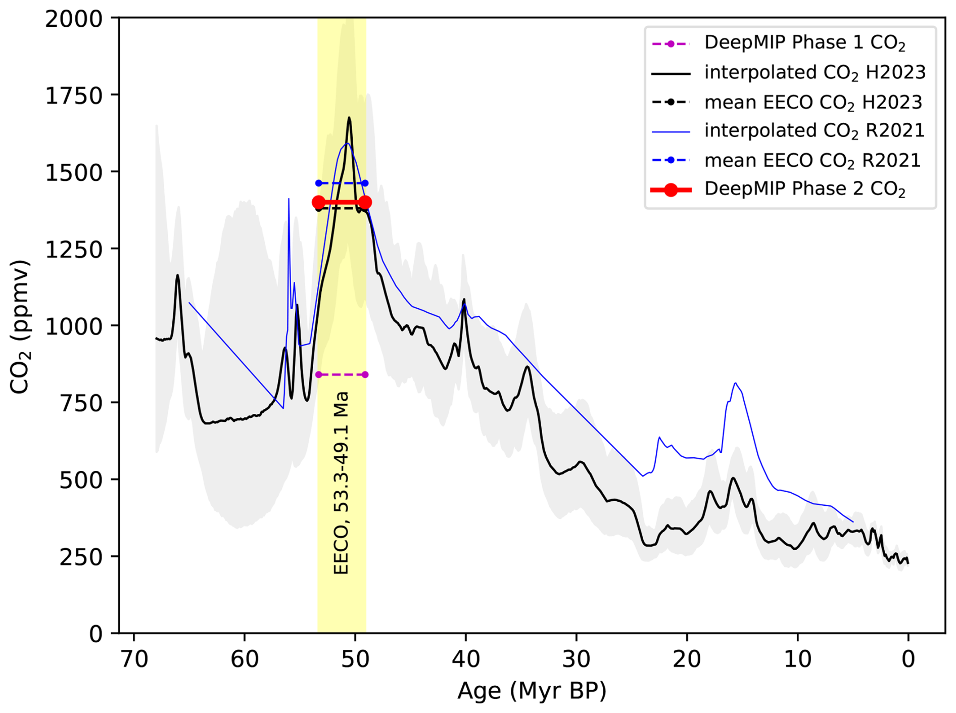
Figure 2 Construction of the standard DeepMIP-Eocene Phase 2 CO₂ concentration. Black solid line shows the Hönisch et al. (2023) (H2023) CO₂ record, with grey shading showing the 95 % confidence interval. Blue solid line shows the Rae et al. (2021) (R2021) CO₂ record. Black and blue dashed lines shows the respective means of the H2023 and R2021 records over the EECO period, 53.3 to 49.1 Ma. Red solid line shows the DeepMIP-Eocene Phase 2 CO₂ of 1400 ppmv (5×PI). Magenta dashed line shows the standard CO₂ concentration in DeepMIP-Eocene Phase 1 (3×PI).

We note that CO₂ of 5×PI under Eocene conditions may lead to crashes or “runaway” warming (i.e. an unphysical non-linear increase in global mean temperature) for some models (Lunt et al., 2021; Zhu et al., 2024). In this case, we encourage the modelling groups to apply the highest CO₂ their model can use in order to have a stable simulation (typically assessed by the surface and/or deep ocean temperature trends, and top-of-model net radiation; see Sect. 2.4). In addition, we encourage the modelling groups to report the CO₂ and temperature levels at which the model crashes frequently or “runs away”.

2.2.2 Paleogeography boundary conditions

The paleogeography (including land-sea mask) used in DeepMIP-Eocene Phase 1 was that of Herold et al. (2014), shown in Fig. 3a. This paleogeographic reconstruction was an update of Markwick (2007), designed to be appropriate for 55 Ma, and relied on the global plate tectonic model of Müller et al. (2008) placed in the mantle (specifically, hotspot) frame of O'Neill et al. (2005). Files were also provided for the same paleogeography, but placed in the paleomagnetic reference frame of Torsvik et al. (2012), and an independent second paleogeography was provided by Getech Plc.

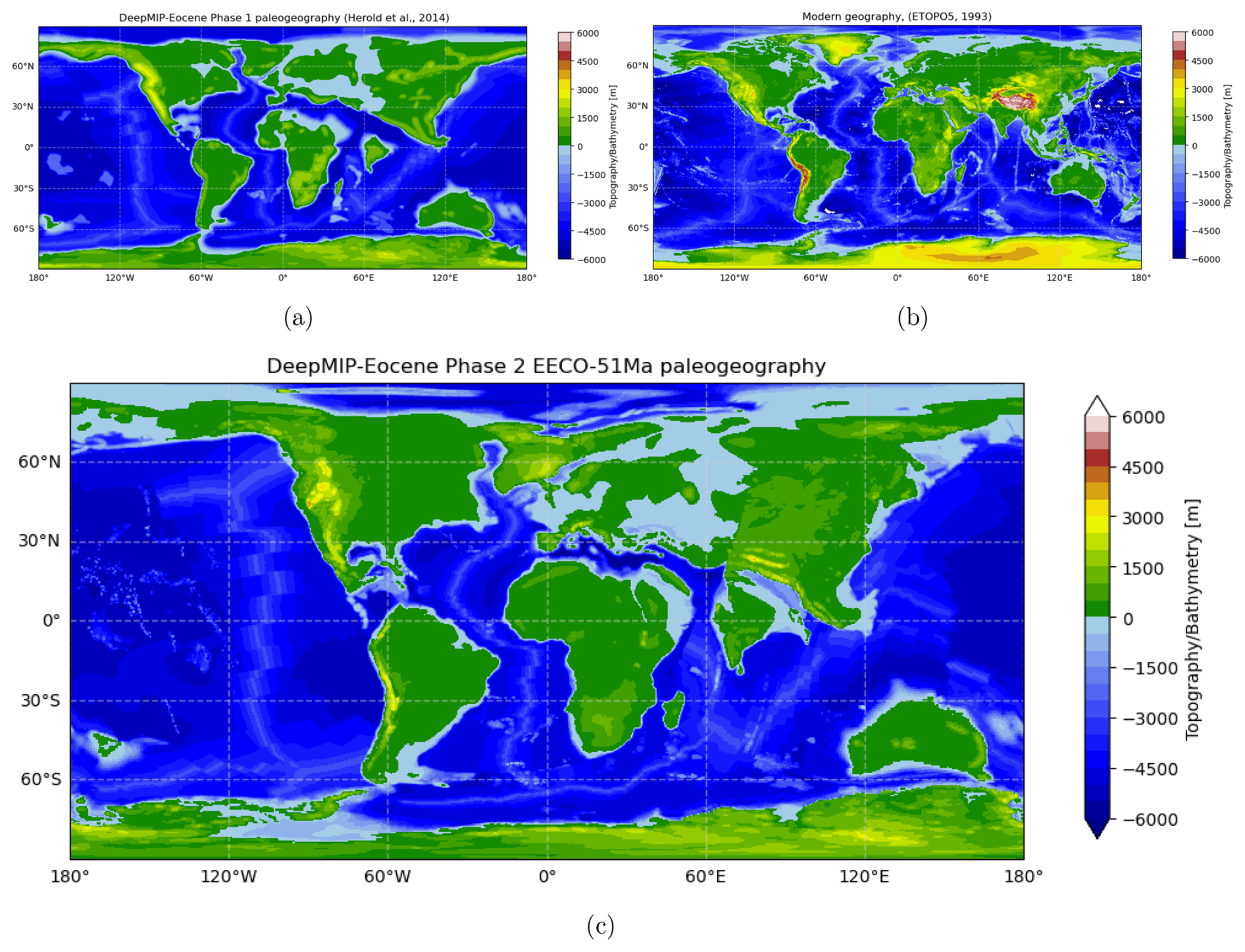
Figure 3 (a) The 55 Ma Herold et al. (2014) paleogeography used in DeepMIP-Eocene Phase 1. (b) The modern geography from ETOPO5 (National Geophysical Data Center, 1993). (c) The 51 Ma DeepMIP-Eocene Phase 2 paleogeography.

For Phase 2, we provide a fully updated paleogeography that builds on recent advances and updates in paleogeographic reconstruction of the Eocene. Since 2014, several studies published new paleogeographic reconstructions for the early Eocene, including Scotese and Wright (2018), He et al. (2019), Straume et al. (2020) with minor updates in Straume et al. (2024), and Aminov et al. (2023). Although these reconstructions are global, the authors often focused on specific regions that were reconstructed in more detail, while other regions were left unchanged from earlier work or simply retained their present-day topography (see Fig. A1). Given the different methods and underlying data used to construct them, it is problematic to assess which reconstruction is “best”. Here, we take a pragmatic approach and integrate the most detailed paleogeographic reconstructions per continent in a new paleogeography for the early Eocene (∼51 Ma).

As a basis, we use the global plate model of Zahirovic et al. (2022) placed in a paleomagnetic reference frame (anchored plate ID = 701701). This plate reconstruction is the current default model in the widely used GPlates software (Müller et al., 2018) and is the same as that being used in DeepMIP-Miocene Phase 2 (Burls et al., 2026). The paleomagnetic reference frame is from Merdith et al. (2021), based on the approach outlined in Tetley et al. (2019). We account for differences in the underlying plate tectonic model of each paleogeography reconstruction used here by rotating them, prior to their incorporation, into the Zahirovic et al. (2022) plate model (and associated reference frame) at 51 Ma, corresponding to the EECO.

We have integrated different regional reconstructions as follows. We incorporate global paleobathymetry at 51 Ma using the method described in Wright et al. (2020) applied to the Zahirovic et al. (2022) plate model (including paleo-oceanic age grid) to ensure self-consistency. For Antarctica, we adopt the “maximum” topographic reconstruction for 34 Ma (Eocene–Oligocene boundary) from Paxman et al. (2019), which provides an update of the ANTscape reconstruction for 34 Ma (Wilson et al., 2012) used in Herold et al. (2014). We retain the reconstruction of Australia and Zealandia from Herold et al. (2014) and preserve the reconstruction of the southern hemisphere gateways of Phase 1, as in Herold et al. (2014). This means that both the Drake Passage and Tasman Gateways are open but shallow, preventing any deepwater throughflow. For South America and the Caribbean region, we rely on the reconstruction of Aminov et al. (2023) for 50 Ma, except for the Andes, where we use the detailed reconstruction from Boschman (2021). We include an updated version of the 50 Ma reconstruction of Aminov et al. (2023) for India and eastern Asia, that includes a more realistic position of the Burma terrane and extent of Greater India based on the India-Asia collision scenario of Westerweel et al. (2025). The reconstruction of the Tibetan region, with its three narrow mountain ranges and intermontane valleys, corresponds to the early Eocene paleo-elevation model of Spicer et al. (2025). For Africa and North America, we integrate the recently published reconstruction of Montheil et al. (2026), which builds upon the work of Poblete et al. (2021) and Aminov et al. (2023). The African topography reflects the middle Eocene (48-41 Ma) and is based on the paleo-facies maps of Couvreur et al. (2021). For North America, Montheil et al. (2026) modified the earlier early-middle Eocene reconstructions that included a long, ∼4 km-high plateau in the North American Cordillera, producing a more realistic topography. Finally, we adopt the reconstruction of Straume et al. (2020, 2024) for the western Tethyan region, western Eurasia and the Arctic (including Greenland). These authors provided a detailed study of the northern hemisphere gateways: in this reconstruction, there is no connection between the Arctic and Pacific Oceans, or between the Arctic and Labrador Sea. The Arctic Ocean is connected to the Neo-Tethys through the West Siberian Seaway (Straume et al., 2024). We include a shallow connection between the Arctic and Atlantic Oceans through the Barents Sea, Norwegian Sea, and North Sea. This represents a maximum connectivity scenario for ∼50–48 Ma with water exchange between the northeast Atlantic and Arctic, supported by the widespread occurrence of the Azolla fern in the Arctic and Nordic seas (Brinkhuis et al., 2006).

As in Phase 1, the land-sea mask is defined as the zero contour of the paleogeography. As all the paleogeographic reconstructions used here have modified the paleo-coastlines after sea level corrections, we do not make an additional explicit sea level correction during our merging process. One exception here is for the Paxman et al. (2019) Antarctica paleotopography, which is reconstructed relative to modern-day sea level – here we incorporate a sea level adjustment based on Wright et al. (2020). We made minor adjustments to regions where two paleogeographic reconstructions were merged, to avoid artefacts such as sudden jumps in topography or bathymetry. We also smoothed one region of very high isolated topography in the Straume et al. (2024) reconstruction east of Greenland. In addition, we removed most interior lakes/seas and very small islands to minimize the manual adjustments needed after re-gridding the map to model resolution.

The resulting DeepMIP-Eocene Phase 2 paleogeography is shown in Fig. 3c, and provided as a NetCDF file on Zenodo (Lunt, 2025b). The map is provided at a relatively high resolution of 0.25°×0.25° (compared to 1°×1° in Phase 1), to allow high resolution atmosphere-only simulations to be carried out (see Sect. 2.3.4), and to allow sub-gridscale topography to be calculated (see below).

Besides the switch to a paleomagnetic reference frame, the main difference between the Phase 2 paleogeography and that of Herold et al. (2014) is that the continental interiors are generally lower in the Phase 2 topography. This is because Herold et al. (2014) built upon the reconstruction of Markwick (2007), whose reconstruction approach generated some anomalously high plateaus in continental interiors. This becomes evident from the fact that the Herold et al. (2014) Eocene topography is substantially higher (in places > 1 km) than modern in the Rockies, India, southern Africa, and much of southeast Asia (see Fig. A1). Another important difference is the reduced width of the Neo-Tethys Ocean. This follows from the change of the reconstruction age from 55 to 51 Ma, during which Africa, and particularly India, have moved farther north relative to Eurasia. There are also changes in the extent of shallow seas, with a reduction in northern Afro-Arabia in Phase 2 compared with Phase 1, and an increase north of India. Correct representation of these shelves could be particularly important for models which incorporate biogeochemistry. There is a more detailed representation of small-scale island features, in particular in the Tethys, which could be important for correctly representing flow through gateways in models with high resolution in the ocean.

For some lower-resolution models, some ocean gateways may not be fully resolved, resulting in them being closed or shallow when they should be open or deep, or vice-versa. Some groups may need to manually adjust gateways accordingly. In this regard, groups should particularly ensure that the Tasman, Drake, Tethys, and Panama gateways are all open, and that there is a connection between the Atlantic and the Arctic oceans. Note that the Tasman, Drake, and Arctic gateways are all relatively narrow and shallow, but are open in this reconstruction.

In addition to the absolute paleogeography, some climate models may require sub-gridscale topography to be prescribed, in particular for gravity-wave drag parameterisations. If this is the case, then modelling groups should implement subgridscale fields as they see fit. A typical approach previously used in Phase 1 is to correlate subgridscale parameters with absolute heights for the modern (outside of Antarctica), and then apply the resulting functions to the absolute Eocene topography to generate the required Eocene sub-gridscale fields. See Sect. 4.2.1 of Lunt et al. (2017) for more details. An alternative approach is to calculate subgridscale topographies directly from the Eocene paleogeography, but care must be taken that the resulting Eocene subgridscale topographies are consistent with those of the preindustrial simulation.

We leave it to individual groups to decide how best to implement any necessary river-runoff routing field, as the format and requirements for such a field are very model-specific. A typical approach is to derive the routing field from the paleogeographic reconstruction (sometimes after interpolation to the model resolution), for example by following the path of steepest descent from each gridcell, until the coast is reached. Of key importance is that the approach taken, and resulting routing field, is documented by each group. We also note that Herold et al. (2014) provided an Eocene runoff routing field in their Supplementary Information, which could be adapted to the new paleogeography in Phase 2, although care should be taken doing this given the differences in topography and land-sea mask compared with the Phase 2 paleogeography.

Diapycnal mixing in the interior of the ocean is primarily driven by internal tides. The magnitude and distribution of the strength of tidal mixing is related to ocean geometry, and would therefore have been different to modern in the Eocene ocean (Green and Huber, 2013). Models often use prescribed values for mixing parameters and mixing parameterisations, and Ladant et al. (2024) have shown that using Eocene-specific tidal mixing can influence ocean circulation, and could potentially be important for correctly representing associated biogeochemical processes. Groups wishing to implement Eocene-specific tidal mixing in their simulations can use the energy dissipation field provided in the Supplementary Information of Herold et al. (2014) (interpolated to the new paleogeography, again taking care given the differences in topography and land-sea mask compared with the Phase 2 paleogeography), which was based on the work of Green and Huber (2013).

In order to facilitate future model-data comparisons, we provide the paleo locations of the sites in the DeepMIP-Eocene proxy database (Hollis et al., 2019; Inglis et al., 2020a) in the new reference frame as an Excel file on Zenodo (Lunt, 2025b). In addition we provide a utility for rotating fields between reference frames (see Code Availability section). The GPlates web service may also be used for retrieving paleo locations consistently with the Phase 2 paleogeography, e.g. to find the paleo location at 51 Ma of a modern site at longitude 32.2° E, 48.9° N, access: https://gws.gplates.org/reconstruct/reconstruct_points/?lons=32.2&lats=48.9&time=51&model=ZAHIROVIC2022&anchor_plate_id=701701 (last access: 3 July 2026).

2.2.3 Vegetation boundary conditions

The vegetation in DeepMIP-Eocene Phase 1 was that of Herold et al. (2014). This was produced by running the BIOME4 vegetation model (Kaplan et al., 2003) forced by a pre-DeepMIP Eocene CESM simulation, with the results expressed using the megabiome classification of Harrison and Prentice (2003) (Fig. 4a).

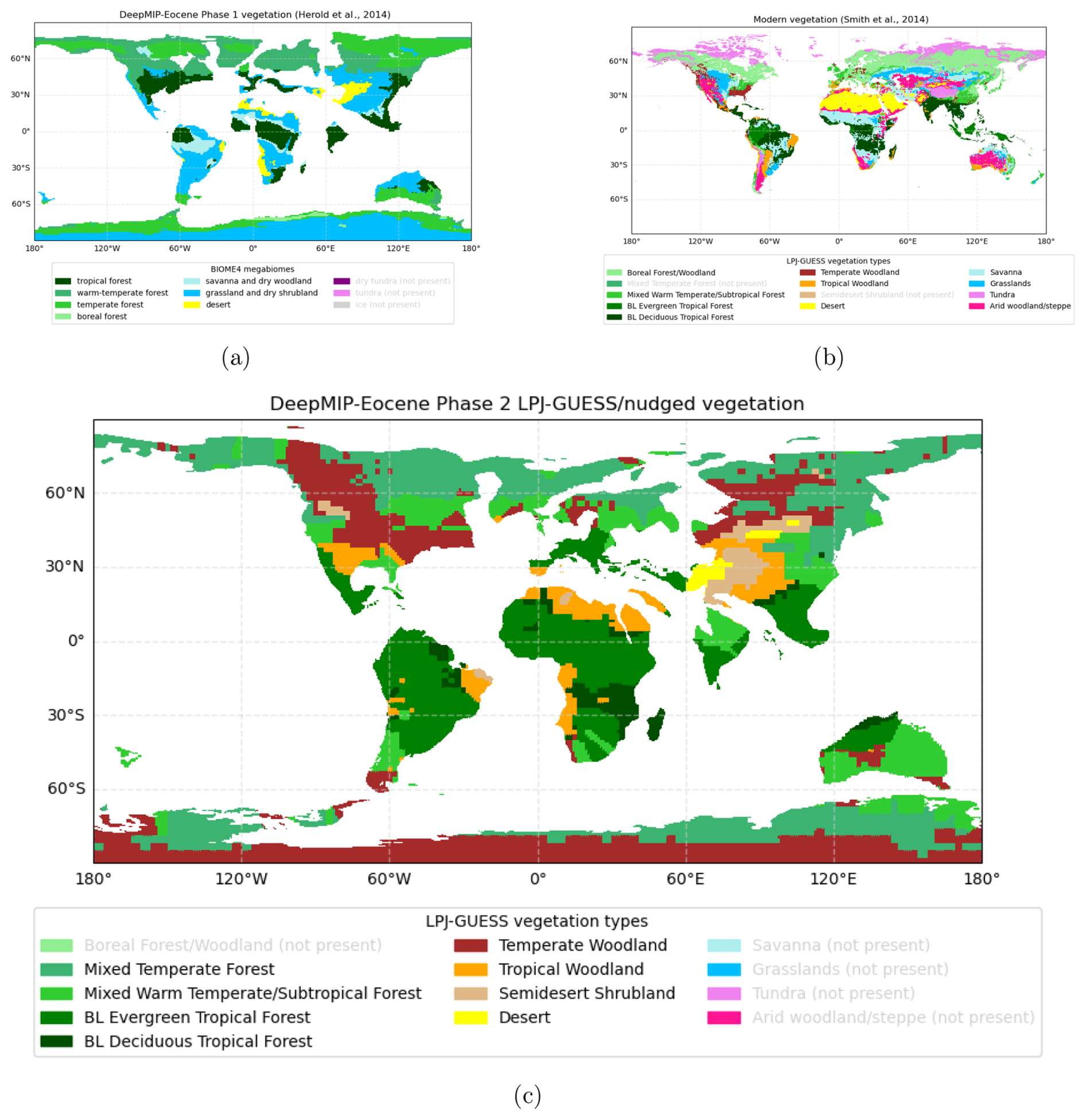
Figure 4 (a) The Herold et al. (2014) vegetation used in DeepMIP-Eocene Phase 1. (b) The modern vegetation of Smith et al. (2014), using LPJ-GUESS biomes which have had minor classification adjustments compared to Smith et al. (2014) in order to increase consistency with the Eocene biomes. (c) DeepMIP-Eocene Phase 2 vegetation, which is derived from the LPJ-GUESS model when forced by the CESM1.2 and GFDL 6×PI simulations from Phase 1 of DeepMIP-Eocene, and nudged towards the vegetation proxy data of Thompson et al. (2025). Note that boreal forests, savannah, grasslands, and tundra vegetation types are not present in the Eocene LPJ-GUESS-based reconstruction in (c), but are included in the legend for comparison with the modern vegetation reconstruction in (b). Figure A2c shows the nudged vegetation in (c) prior to being regridded to the DeepMIP-Eocene Phase 2 reference frame and land-sea mask.

For Phase 2, we make use of work of Brugger et al. (2026), who ran the LPJ-GUESS vegetation model (Smith et al., 2014) forced by all of the DeepMIP-Eocene Phase 1 climate model simulations. To better represent Eocene vegetation, plant functional types were adjusted in these simulations by adding shrub plant functional types based on Allen et al. (2020) and deactivating grass plant functional types. Qualitative comparison (Brugger et al., 2026) of these results with a proxy paleoflora dataset of the Eocene (Thompson et al., 2025) indicates best agreement between the model simulations and data for vegetation associated with the CESM1.2 simulation at 6×PI over most of the globe (see Fig. A2a), but a best fit with vegetation associated with the GFDL simulation at 6×PI over Antarctica (see Fig. A2b). Therefore, we choose this hybrid CESM1.2/GFDL-forced LPJ-GUESS vegetation distribution as the starting point for the boundary condition for DeepMIP-Eocene Phase 2.

To produce the final data-model hybrid vegetation boundary condition, we integrated the palaeobotanical data-based reconstruction published in Thompson et al. (2025) with the CESM1.2/GFDL-forced LPJ-GUESS model-based vegetation simulation (Brugger et al., 2026). Following the qualitative approach established within the PlioMIP framework (Salzmann et al., 2008), manual adjustments were made for regions where palaeobotanical data showed substantial discrepancies with the model simulations. These adjustments include extending warm-temperate forest cover in East Asia, replacing boreal forest with temperate forests in West Siberia, and increasing the extent of dry woodlands in northern hemisphere subtropical regions (see Fig. A2c). However, we note that there is geographical bias in the quantity of paleobotanical data, with for example relatively dense coverage in western North America and southeast Asia, but no coverage in the region of the modern Amazon (Fig. A2). The hybrid vegetation was then regridded to the new Phase 2 land-sea mask – the final result of this process is shown in Fig. 4c.

We note that the CO₂ of 6×PI in the underlying LPJ-GUESS vegetation model simulations is inconsistent with the 5×PI recommended in the DeepMIP-Eocene Phase 2 climate model simulations and based on CO₂ proxies. However, 5×PI simulations are not available from the last phase of DeepMIP-Eocene, and in any case, biases in the climate sensitivity of the climate models could result in an inconsistency between actual Eocene CO₂ and the CO₂ that results in the best modelled fit to the vegetation data.

Similarly as for Phase 1, it is important that groups take care to implement this vegetation in a manner as consistent as possible with their preindustrial control simulation. This may mean converting the LPJ-GUESS vegetation types into the model's intrinsic vegetation types, or converting the LPJ-GUESS vegetation types into land surface parameters such as albedo, roughness length etc. In either case, a modern map of vegetation, using the LPJ-GUESS vegetation types, is provided as a NetCDF file on Zenodo (Lunt, 2025b) to aid this process, and shown in Fig. 4b. Values of several land-surface parameters for typical vegetation types are available on the PRISM webpages: https://geology.er.usgs.gov/egpsc/prism/prism_1_23/ancillary/Biome_Megabiome_Lookup.html (last access: 3 July 2026).

2.2.4 Other boundary conditions

The recommendation for all other boundary conditions remains unchanged from Phase 1 (refer to Lunt et al., 2017). Using the section numbering from Lunt et al. (2017), detailed recommendations are given therein for soils and lakes (Sect. 4.2.2), non-CO₂ greenhouse gases (Sect. 4.2.3), aerosols (Sect. 4.2.4), and solar luminosity and astronomical (orbital) parameters (Sect. 4.2.5). In brief, soil parameters are globally homogeneous typical modern values, there are no lakes or ice sheets, non-CO₂ greenhouse gas concentrations are kept as preindustrial, several options are provided for aerosols, and solar luminosity and astronomical configurations are kept as modern. Due to the uncertainties in many of these aspects, suggested sensitivity studies are highlighted below.

2.3 Suggested sensitivity studies

Groups are encouraged to carry out any sensitivity studies in which they are interested, and that best advance their scientific understanding. Sometimes, it can be useful to have more than one group carry out a particular sensitivity study, to test model dependence. We therefore suggest some sensitivity studies that may be of particular interest, and provide NetCDF files on Zenodo (Lunt, 2025b) as appropriate. The names of the sensitivity simulations are summarised in Table 1.

2.3.1 Sensitivity studies to greenhouse gases and solar luminosity; simulations deepmip-eocene-p2-YxCO2, deepmip-eocene-p2-5xCO2-solmeth, equilibrium-4xCO2

As described in Sect. 2.1, one of the mandatory experiments in DeepMP Phase 2 is a sensitivity study with 1×PI, to identify the impact of CO₂ versus non-CO₂ forcings on Eocene climate (simulation deepmip-eocene-p2-1xCO2, see Table 1). In addition, we encourage EECO sensitivity studies at other CO₂ concentrations (simulations deepmip-eocene-p2-YxCO2, see Table 1), including 4×PI (also allowing comparison with an extended/equilibrated version of the CMIP abrupt-4xCO2 experiment; equilibrium-4xCO2, see Table 1), 3×PI (also allowing comparison with the most common Eocene simulation from Phase 1), and 6×PI (close to the top-end estimate of EECO CO₂ from Hönisch et al., 2023 and Rae et al., 2021). These sensitivity simulations with various CO₂ levels could also be used to examine the potential nonlinearity in the sensitivity of Eocene temperatures to CO₂ (Zhu et al., 2019; Caballero and Huber, 2013). We also encourage abrupt CO₂ changes to estimate the ECS of the Eocene configuration (in particular an abrupt quadrupling from 1×PI to 4×PI for comparison with the modern abrupt-4xCO2 experiment).

Given that there is evidence that there were more wetlands in the Eocene compared with modern (Wilton et al., 2019), and that there were perturbations to the CH₄ cycle during the PETM (Inglis et al., 2020b), it is probable that CH₄ concentrations during the EECO were higher than modern. For DeepMIP-Eocene Phase 1, Lunt et al. (2017) justified keeping non-CO₂ greenhouse gases as preindustrial and solar luminosity as modern, by arguing that their respective forcings broadly cancelled out. However, this neglects the substantial uncertainty in Eocene CH₄ (and other non-CO₂ greenhouse gas) forcing, and neglects that even if these two forcings balance in the global annual mean, seasonal and spatial residuals in the climate response will still remain (Lunt et al., 2008). We therefore encourage sensitivity studies in which changes in solar luminosity and CH₄ are separately represented (simulation deepmip-eocene-p2-5xCO2-solmeth, see Table 1). For solar luminosity we recommend the value of 1355 W m⁻² for 51 Ma (Gough, 1981). For CH₄, a value of 3000 ppb for the early Eocene is consistent with the modelling work of Beerling et al. (2011). This was the value calculated in Lunt et al. (2017) to roughly cancel the solar luminosity change, see their Sect. 4.2.3. However, Beerling et al. (2011) also quotes a range between 2580–3614 ppb, so other values may be preferred.

2.3.2 Sensitivity studies to paleogeography; simulations deepmip-eocene-p2-5xCO2-geogherold and deepmip-eocene-p2-5xCO2-geog56Ma

Some groups may wish to explore the difference between the Phase 1 paleogeography of Herold et al. (2014) and the new Phase 2 paleogeography (simulation deepmip-eocene-p2-5xCO2-geogherold; Table 1). We therefore provide the Herold et al. (2014) paleogeography on the new Phase 2 reference frame (at 55 Ma for consistency with the original Herold et al. (2014) reconstruction) as a NetCDF file on Zenodo (Lunt, 2025b) (Fig. 5a), because the reference frame has been shown to influence atmospheric and ocean circulation (Baatsen et al., 2018; Zhang et al., 2024).

Some groups may wish to simulate the PETM (56 Ma) as opposed to the EECO (51 Ma) (simulation deepmip-eocene-p2-5xCO2-geog56Ma; Table 1). As such, we provide a version of the Phase 2 paleogeography that has been rotated back to 56 Ma, consistently with the Phase 2 plate model and reference frame, and including topography specific to 56 Ma in South America (Boschman, 2021) and the North Atlantic region (Straume et al., 2024), as a NetCDF file on Zenodo (Lunt, 2025b) (Fig. 5b).

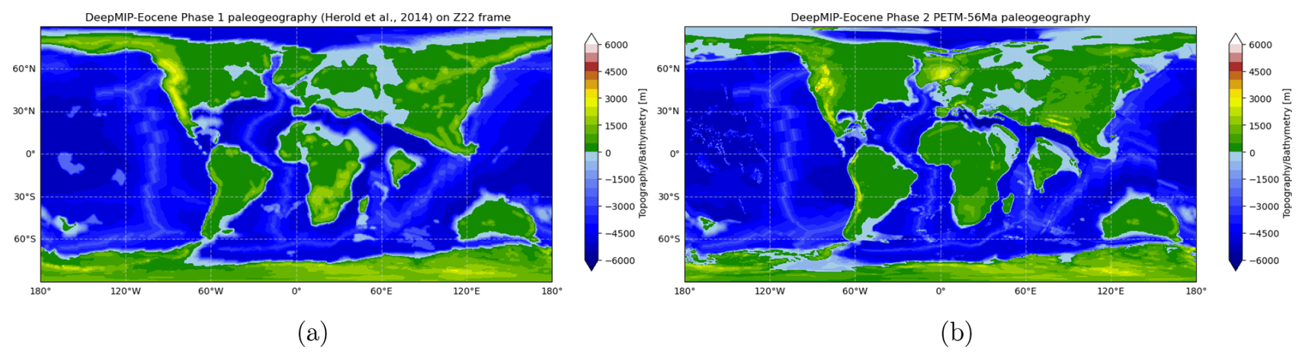
Figure 5 (a) The Herold et al. (2014) paleogeography, at 55 Ma on the Phase 2 plate model and reference frame, suggested as a sensitivity study in DeepMIP-Eocene Phase 2 (simulation deepmip-eocene-p2-5xCO2-geogherold; Table 1). For comparison with the standard DeepMIP-Eocene Phase 2 paleogeography in Fig. 3c and the original Herold et al. (2014) paleogeography in Fig. 3a. (b) 56 Ma paleogeography suggested as a sensitivity study in DeepMIP-Eocene Phase 2 (simulation deepmip-eocene-p2-5xCO2-geog56Ma; Table 1). For comparison with the standard DeepMIP-Eocene Phase 2 paleogeography in Figu. 3c.

2.3.3 Sensitivity studies to vegetation and land surface parameters; simulation deepmip-eocene-p2-5xCO2-vegthompson

An alternative Phase 2 vegetation dataset is provided by Thompson et al. (2025). In this case, a similar approach is taken as in Brugger et al. (2026), but the BIOME4 vegetation model (Kaplan et al., 2003) is used in place of the LPJ-GUESS model. Thompson et al. (2025) find that the vegetation associated with the CESM1.2 and GFDL_CM2.1 models at 6×PI best fit the vegetation proxy data, which is consistent with the findings of Brugger et al. (2026) using LPJ-GUESS. Given that the CESM1.2 model (Hurrell et al., 2013) runs at a higher horizontal and vertical resolution than the GFDL_CM2.1 model (Delworth et al., 2006) and was developed more recently, and is therefore likely to overall have a more accurate representation of physical processes, we use the CESM1.2-based vegetation as the main sensitivity study in DeepMIP-Eocene Phase 2. Again, we note that this CO₂ concentration is inconsistent with the 5×PI recommended in the DeepMIP-Eocene Phase 2 climate model simulations. We encourage groups to carry out sensitivity studies using this Thompson et al. (2025) vegetation, which is shown in Fig. 6a. However, in contrast to our LPJ-GUESS model/proxy hybrid reconstruction (and the underlying LPJ-GUESS vegetation), this BIOME4 vegetation shows widespread discrepancies in the subtropics and mid-latitudes between proxy-reconstructed forests and woodlands and modelled dry shrublands and deserts (Thompson et al., 2025). Similarly as for the LPJ-GUESS vegetation, a modern vegetation map using the BIOME4 vegetation types is provided (Fig. 6b, see Sect. 4.2.2 of Lunt et al., 2017 for more details).

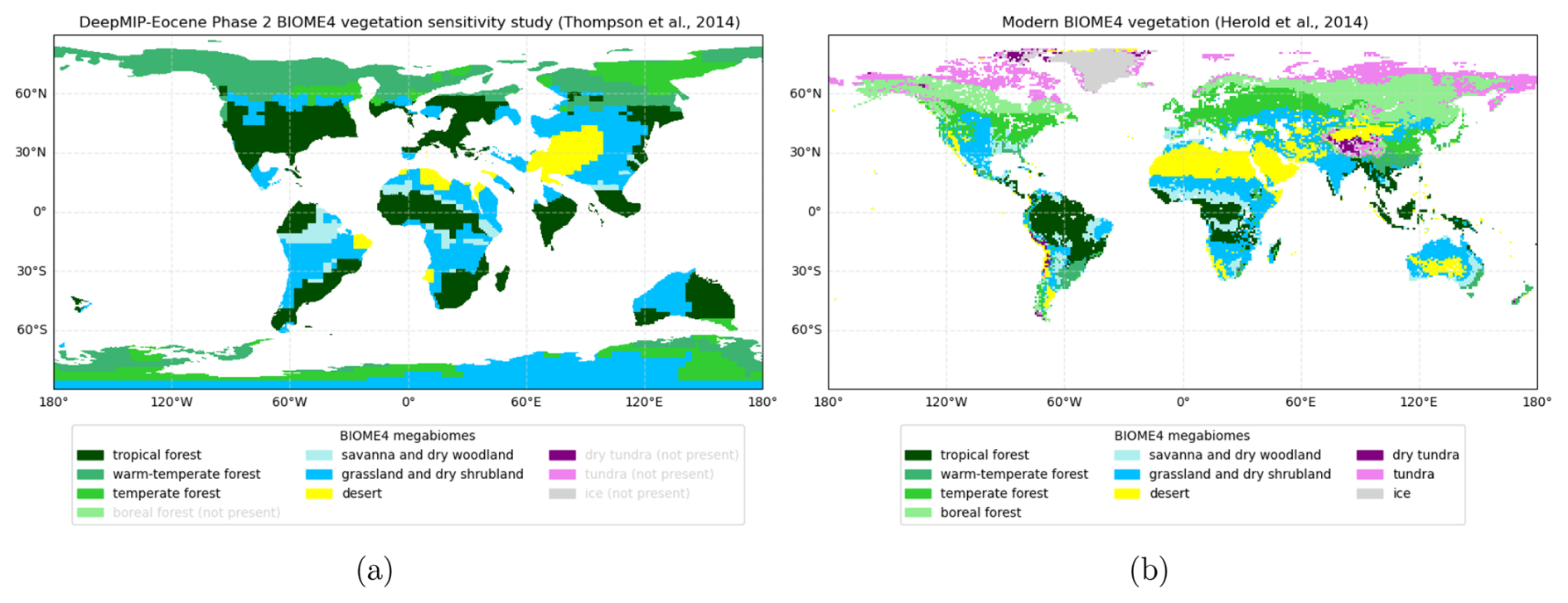
Figure 6 (a) The Thompson et al. (2025) vegetation, suggested as a sensitivity study in DeepMIP-Eocene Phase 2 (simulation deepmip-eocene-p2-5xCO2-vegthompson; Table 1), which is the output of the BIOME4 model when forced by the CESM1.2 6×PI simulations from Phase 1 of DeepMIP. For comparison with the standard DeepMIP-Eocene Phase 2 vegetation in Fig. 4c. (b) Modern vegetation using the same biome classification as BIOME4 (Herold et al., 2014).

Furthermore, we encourage sensitivity studies to lake distributions, as these have been shown to be potentially important for determining Eocene hydrology and climate, through changes in surface heat capacity and formation of low clouds (Henry and Vallis, 2022). Similarly, modified Eocene soil characteristics are likely to play a role, given their impact on warm climate simulations of the Pliocene (Pound et al., 2014). Although there are global maps of soils and lakes for the Pliocene based on proxy data (Pound et al., 2014), no such global datasets exist for the early Eocene as far as we are aware. As such, Eocene sensitivity studies are likely to be somewhat idealised, but could be modified in association with the vegetation types, as is defined for DeepMIP-Miocene (Bradshaw et al., 2025).

2.3.4 Other sensitivity studies

Groups are of course welcome to carry out sensitivity studies in addition to those in Table 1. As in Phase 1, we encourage sensitivity studies to astronomical (orbital) parameters (see Ross, 2023 and Sect. 4.3.3 in Lunt et al., 2017), and to initialisation (Sect. 4.3.7 in  Lunt et al., 2017). Other aspects that groups may wish to explore include: aerosols (Kiehl and Shields, 2013), atmospheric chemistry, including for example methane–ozone–hydroxyl interactions (Beerling et al., 2011), model resolution (Nooteboom et al., 2022), dynamic vegetation (Loptson et al., 2014), tidal mixing (Ladant et al., 2024), stable water isotopes (Zhu et al., 2020), and internal model parameters (Sagoo et al., 2013). Groups may also wish to carry out high-resolution atmosphere-only simulations to explore processes/features such as atmospheric rivers (Shields et al., 2021).

2.4 Initial conditions, integration length, and assessment of equilibrium

In Phase 1, a recommendation was given for oceanic temperature and salinity initial conditions. This was a linear decrease of temperature with depth, as a function of latitude, and a globally constant salinity of 34.7 psu (see Eq. 1 in Lunt et al., 2017). However, several groups found that the model became unstable with this initial condition, and other groups found that it resulted in very long spinup times, as the linear decrease with depth resulted in an excess of energy at intermediate depths which took a long time to dissipate. As such, in Phase 2 we are less prescriptive, and encourage groups to use their preferred method for initialisation. The key requirement is that groups clearly document their method in their respective publications.

As an example, groups may choose to initialise from spun-up oceanic states from previous Phase 1 simulations, carried out with their own or other models, and available in the DeepMIP-Eocene Phase 1 model database (Steinig et al., 2024). In this case, we encourage groups to use appropriate initial conditions according to the CO₂ concentration at which they are running (see discussion in Steinig et al., 2026), and accounting for the climate sensitivity of their model compared with the climate sensitivity of the initialising model. Also in this case we recommend that groups take account of any residual TOA imbalance in the previous simulations as a broad indicator of their degree of equilibration (see Table S1 in the Supplement of Lunt et al., 2021).

Alternatively, groups may wish to use ocean proxy data to inform the initialisation of the temperature and salinity fields. In particular, deep ocean clumped isotope data (Meckler et al., 2022) using the calibration of Meinicke et al. (2020), and a pH-adjusted transformation to temperature of the benthic oxygen isotope record (Westerhold et al., 2020; Evans et al., 2024), constrain EECO deep ocean temperature to 16.2±4.4 and 18.4±0.6 °C (1 SD), respectively (Fig. 1). We therefore suggest that simulations could be initialised with a deep ocean temperature of around 17 °C, intermediate between these two approaches (although we note that there are uncertainties in this value associated with uncertainties in the calibrations). Analysis of the phase one DeepMIP model output (Goudsmit-Harzevoort et al., 2023) demonstrated that the inter-basin deep ocean temperature offset is less than 0.5 °C, and that the temperature gradient in the deep ocean is less than 0.5 °C km⁻¹ in the majority of the simulations included in that analysis, as is also the case for the modern ocean. However, although at present there is no evidence for strong inter-basin heterogeneity in deep ocean temperature in the EECO, we note evidence for stronger (>4 °C) deep ocean heterogeneity in past warm periods such as the mid-Pliocene (Braaten et al., 2023). Overall, despite these uncertainties, we suggest that the above initialisation temperature be applied to all basins and depths below 3 km.

In any case, we strongly recommend that groups initialise temperature and salinity in a mutually consistent fashion, to avoid spurious density contrasts early in the simulation, and that groups initialise with relatively warm temperatures in the deep ocean, because doing so may potentially accelerate spin-up by enabling the activation of a meridional overturning circulation more quickly, as opposed to remaining stratified for a relatively long time due to a “cold-start”.

As in Phase 1, simulations should be carried out for as long as possible, in order to reach as close to equilibrium as possible. In Phase 1, a mean absolute TOA imbalance of less than 0.3 W m⁻² was required. Since then, de Boer et al. (2025) have shown that substantial climatological and ocean circulation changes can take place following additional spinup after a threshold of 0.3 W m⁻² has been reached. Therefore, in Phase 2 we strongly encourage groups to aim for a mean absolute TOA imbalance over the final 100 years of the simulations (i.e. the period uploaded to the DeepMIP database) of less than 0.1 W m⁻² and deep ocean temperature (at ∼3500 m) trends of less than 0.1°/century. For those models for which the TOA energy budget is not closed, the TOA imbalance should be similar to that of an equilibrated preindustrial control simulation. These reduced thresholds particularly apply to the “standard” simulations (deepmip-eocene-p2-5xCO2 and deepmip-eocene-p2-1xCO2; see Table 1). We encourage groups to report their extrapolated full-equilibrium temperature as derived from a “Gregory plot” (Gregory et al., 2004). Given that these thresholds are not necessarily sufficient to indicate an ocean circulation in quasi-equilibrium, modelling groups are encouraged to report time series of key ocean variables to enable diagnoses of ocean equilibrium (de Boer et al., 2025) (see Sect. 2.5). Groups may also choose to carry out “ocean surgery” during a simulation (Steinig et al., 2026), in which instantaneous perturbations are applied to the ocean temperature field in an attempt to accelerate the progression towards full equilibrium.

2.5 Model outputs

We strongly encourage groups to upload their simulation boundary conditions and outputs to the DeepMIP database (Steinig et al., 2024). Instructions for uploading data are given here: https://www.deepmip.org/data (last access: 3 July 2026). We encourage groups to provide means and standard deviations of the last 100 years of their simulations for multiple variables, and timeseries of the last 100 years of their simulations for selected variables. Each output variable is stored in a separate file according to the following structure:

$$\begin{array}{ll}{\displaystyle }& {\displaystyle }\mathrm{directory}=\mathtt{deepmip}-\mathtt{eocene}-\mathtt{p}\mathtt{2}/<\mathtt{Family}>/\\ {\displaystyle }& {\displaystyle }<\mathtt{Model}>/<\mathtt{Experiment}>/\\ {\displaystyle }& {\displaystyle }<\mathtt{Version}>/<\mathtt{Averaging}>\\ {\displaystyle }& {\displaystyle }\mathrm{filename}=<\mathtt{Variable}>\mathtt{\_}<\mathtt{Model}>\mathtt{\_}\\ {\displaystyle }& {\displaystyle }<\mathtt{Experiment}>\mathtt{\_}<\mathtt{Version}>.\\ {\displaystyle }& {\displaystyle }<\mathtt{Statistic}>.\mathtt{nc}\end{array}$$

where:

• <Family> and <Model> describe the model used to carry out the simulations (see Table 1 in Steinig et al., 2024, for examples from Phase 1).

• <Experiment> is listed Table 1 of this paper (also see Table 2 in Steinig et al., 2024, for examples from Phase 1).

• <Variable> represents the variable name; we encourage all groups to use CF-compliant (Eaton et al., 2023) variable names. A list of commonly-used variables from Phase 1 is given in Tables 4 (atmosphere) and 5 (ocean) of Steinig et al. (2024). In addition, studies of ocean mixing would benefit from the total vertical diffusivity coefficient (and its contributions, if relevant), the Brunt–Väisälä frequency, and the power consumed by mixing processes. Also, studies exploring the role of isopycnal mixing would benefit from outputs related to ocean eddy parameterisation, for example from the Gent and Mcwilliams (1990) scheme, if used.

• <Statistic> is either “mean” (1 or 12 timesteps for annual or monthly means), “std” (1 or 12 timesteps for annual or monthly temporal standard deviations across the meaning period), “time_series” (1200 timesteps) or omitted for the time-independent boundary conditions.

• <Averaging> can either be “climatology” or “time_series]]. “Climatology” denotes the directory for storing the (smaller) climatological mean and standard deviation (“mean” and “std” files). “time_series” denotes the directory for storing the (larger) “time_series” files to enable more granular download options.

We further strongly encourage modelling groups to upload full simulation-length time series of key oceanic variables to diagnose the equilibrium state of the ocean. These are the mean temperature in the model level that includes a depth of 3500 m, and where available also the mean ocean ideal age tracer at this level. We further encourage the reporting of key meridional overturning circulation (MOC) streamfunction maxima and minima, and suggest specifically the outputs: Atlantic MOC (AMOC): maximum between 45–68° N; Pacific MOC (PMOC): maximum between 25–58° N; Global MOC (GMOC): maximum global MOC north of 40° S; Southern Ocean MOC: absolute of minimum of the GMOC south of 60° S. All metrics should be calculated below 500 m depth to exclude the wind-driven gyres (de Boer et al., 2025). When calculating the overturning streamfunction in specific basins, care should be taken to correctly account for any open lateral boundaries.

For those models with an irregular ocean (and/or atmospheric) grid, in addition to the native grid, the results should also be interpolated to a regular lat–lon grid prior to uploading to the database. In this case, care should be taken that the global mean of relevant variables is conserved.

If the deepmip-eocene-p2-5xCO2 simulation becomes an official CMIP7 simulation (likely named eocene-5x), then we also encourage groups to submit this simulation the Earth System Grid Federation (ESGF).

3 Summary

We have provided a framework for groups to carry out consistent sets of climate model simulations of the early Eocene, facilitating model-data comparisons and exploration of sensitivities. We hope that modelling groups will soon begin to start simulations within this new framework, and have a “stretch goal” to have some simulations available in time for inclusion in IPCC AR7. In any case, we anticipate, as was the case for Phase 1, that this framework will lead on to multiple studies exploring multiple aspects of the Earth system under a high-CO₂ warm climate. Again, as in Phase 1, we anticipate that those scientists who carry out the model simulations will be able to actively contribute to many of these papers, bringing their own expertise about their models to the analysis, and recognising their hard work in configuring and carrying out their simulations. We also anticipate that the DeepMIP proxy database will be expanded and developed over this period, leading to new insights and more robust model-data comparisons.

Appendix A

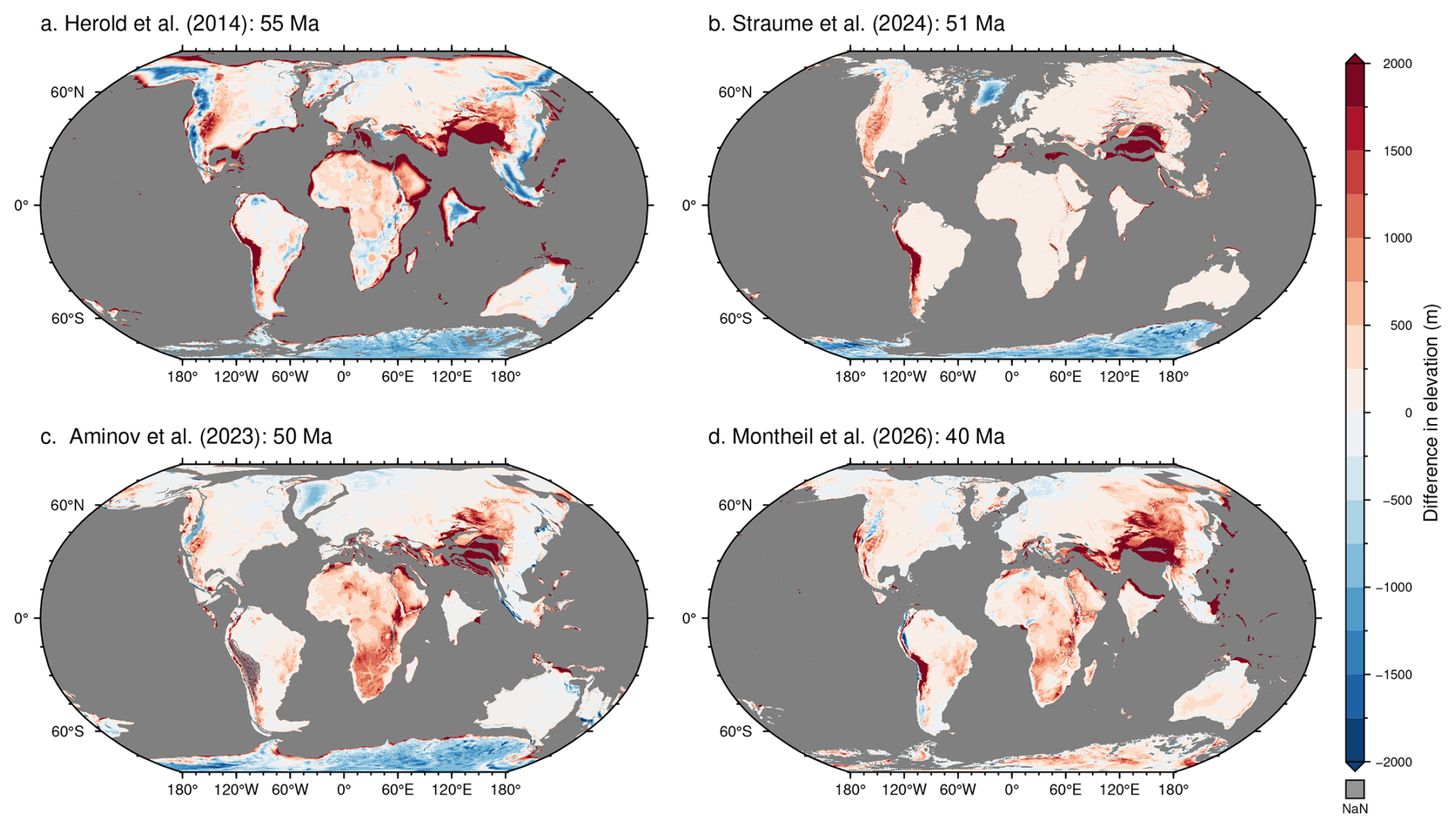
Figure A1 Difference in height between the four Eocene paleogeographies considered in this paper and the modern ETOPO5 geography (National Geophysical Data Center, 1993), ETOPO5 minus Eocene, with the modern geography rotated to the appropriate Eocene time period for each paleogeography.

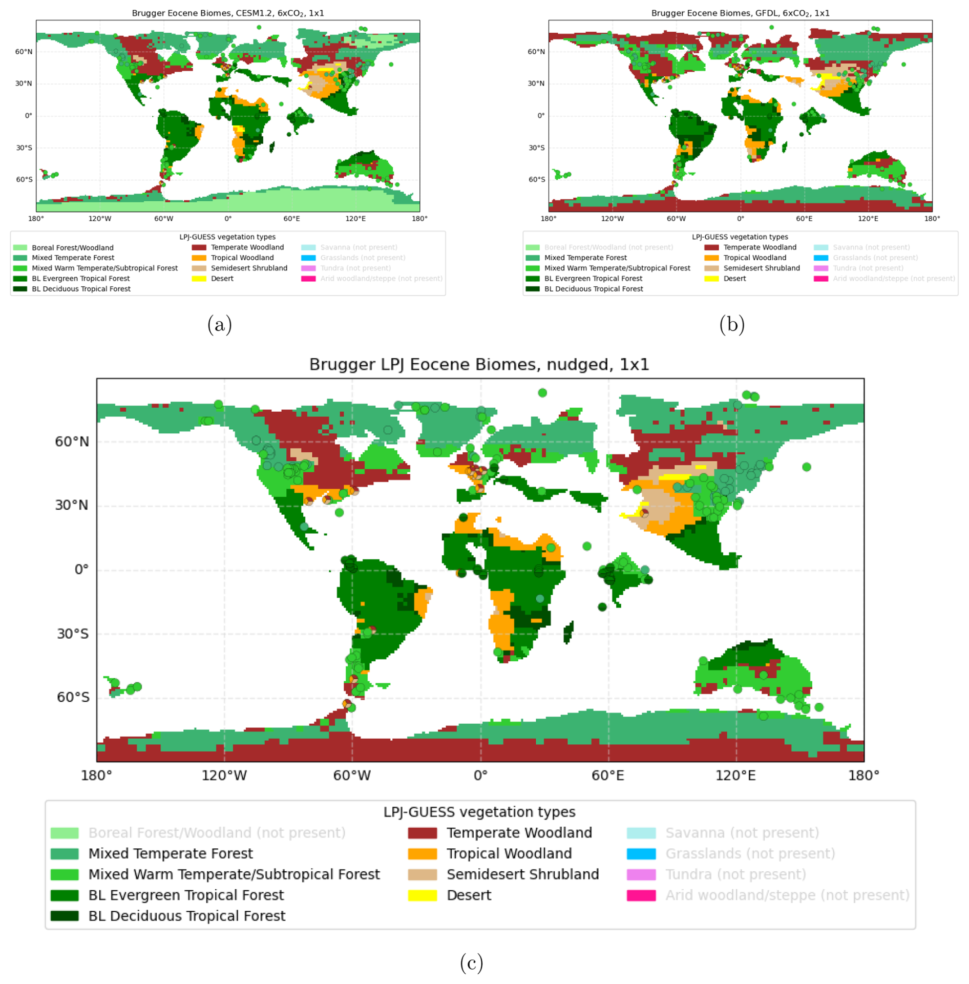
Figure A2 (a) The original vegetation from Brugger et al. (2026), with LPJ-GUESS forced by the DeepMIP Phase 1 simulations from (a) CESM1.2 at 6×PI and (b) GFDL at 6×PI. (c) The hybrid proxy-model reconstruction, which is then regridded to the DeepMIP Phase 2 reference frame, as shown in the main paper in Fig. 4c. Superimposed on all plots is the vegetation proxy data of Thompson et al. (2025).