HyperGas 1.0: a python package for analyzing hyperspectral data for greenhouse gases from retrieval to emission rate quantification

We present HyperGas, an open-source Python package for the retrieval and estimation of atmospheric greenhouse gas concentration enhancements and plume emission rates using data from hyperspectral imagers such as the PRecursore IperSpettrale della Missione Applicativa (PRISMA), the Environmental Mapping and Analysis Program (EnMAP), and the Earth Surface Mineral Dust Source Investigation (EMIT). The software is designed for compatibility with any three-dimensional hyperspectral radiance dataset. HyperGas supports multiple retrieval algorithms, including matched filter and lognormal matched filter, and offers two emission rate estimation methods: the integrated mass enhancement and cross-sectional flux approaches. The software provides a scalable batch-processing framework that supports data workflows from radiances to emission rates and an interactive graphical user interface that enables visualization of gas plumes. Built on high-level data structures such as xarray and CSV, HyperGas simplifies metadata handling and facilitates robust analysis and visualization. The package provides a robust foundation for community use and expansion. This toolkit aims to advance atmospheric monitoring capabilities and support both research and operational applications of greenhouse gas monitoring.

1 Introduction

Greenhouse gases such as carbon dioxide (CO₂) and methane (CH₄) are the primary drivers of anthropogenic climate change, contributing to global warming and altering the Earth’s energy balance (IPCC, 2023). Monitoring these gases at facility-scale is increasingly important for identifying and quantifying emission sources, supporting and verifying mitigation efforts, and informing climate policy. Spaceborne hyperspectral imagers (HSI), with their ability to capture hundreds of narrow, contiguous spectral bands, have been demonstrated to enable the detection and quantification of methane and CO₂ concentrated sources (Guanter et al., 2021; Jacob et al., 2022; Cusworth et al., 2023; Thorpe et al., 2023; Borger et al., 2025; Zhang et al., 2025). However, as no operational greenhouse gas products exist for these missions, such analyses have so far been limited to a few specialized research groups. Furthermore, the analysis requires several steps that can diverge between different analysis groups. To broaden access and facilitate wider scientific use, we introduce an open-source framework for greenhouse gas analysis from HSI data.

Hyperspectral imagers have become a powerful tool for a wide range of remote sensing applications (Qian, 2021). HSIs were originally designed to characterize Earth’s surface features such as mineral distributions. They have high spatial and spectral resolution that also enables the detection of greenhouse gases, most notably CO₂ and methane, under favorable conditions (Thorpe et al., 2023). Their fine spectral resolution (∼10 nm) allows for more accurate detection and quantification of atmospheric greenhouse gases compared to multispectral imaging (∼100 nm; e.g., Sentinel-2 and Landsat) but is still limited compared to area mappers such as Global Observing SATellite (GOSAT) and TROPOspheric Monitoring Instrument (TROPOMI) that allow the precise estimation of background gas concentrations (e.g., Jacob et al., 2022). Over the past two decades, advancements in imaging spectrometer technologies have led to a surge in the availability and quality of spaceborne HSI data. From early missions like Earth Observing-1 (EO-1)/Hyperion (Pearlman et al., 2001) to newer platforms such as GaoFen-5 (Liu et al., 2019), the PRecursore IperSpettrale della Missione Applicativa (PRISMA; Loizzo et al., 2018; Cogliati et al., 2021), the Environmental Mapping and Analysis Programme (EnMAP; Guanter et al., 2015; Storch et al., 2023), the Earth Surface Mineral Dust Source Investigation (EMIT; Green et al., 2020, 2023), and the Carbon Mapper Coalition satellites (Tanager-series; Duren et al., 2025), there has been a steady improvement in spatial, spectral, and temporal resolutions. These instruments have been applied to detect methane and CO₂ emitters around the world (Guanter et al., 2021; Thorpe et al., 2023; Han et al., 2024; Zhang et al., 2025). With upcoming missions like the Copernicus Hyperspectral Imaging Mission for the Environment (CHIME; Rast et al., 2021) and the Surface Biology and Geology mission (SBG; Cawse-Nicholson et al., 2021), researchers and analysts will soon have access to an unprecedented volume of high-resolution hyperspectral data.

Existing open-source tools, such as mag1c (Foote et al., 2020) and emit-ghg (Brodrick et al., 2026), are restricted to a single HSI or data format, while frameworks such as ddeq (Kuhlmann et al., 2024) focus mainly on source quantification rather than a complete end-to-end workflow. To address these limitations, we introduce HyperGas, an open-source Python package designed to streamline greenhouse gas analysis across different HSI datasets. Instead of proposing a new retrieval algorithm, HyperGas combines established matched-filter techniques for gas enhancement retrieval into a unified workflow. It also applies standard integrated mass enhancement (IME) and cross-sectional flux (CSF) methods for emission quantification, enabling consistent application across multiple sensors. The package supports enhancement retrieval, plume detection, masking, uncertainty handling, and emission estimation through both automated batch processing and an interactive graphical user interface. Its modular design also allows users to add additional instruments, incorporate and contribute new algorithms, as well as develop customized processing strategies. In this paper, we present the design principles behind HyperGas, demonstrate its capabilities through a number of real-world case studies involving methane and CO₂, and outline how it can serve as a foundation for reproducible, scalable greenhouse gas analysis using HSI data.

2 Software description

We have designed the HyperGas package for Level 1 (L1, radiance) to Level 4 (L4, e.g., emission rate estimates) products, including the following steps described in Sect. 2.1–2.4 (Fig. 1):

1. Data preparation (L1; Sect. 2.1)

2. Greenhouse gas retrieval (L2; Sect. 2.2)

3. Plume detection and segmentation (Defined here as L3; Sect. 2.3)

4. Emission estimation (L4; Sect. 2.4)

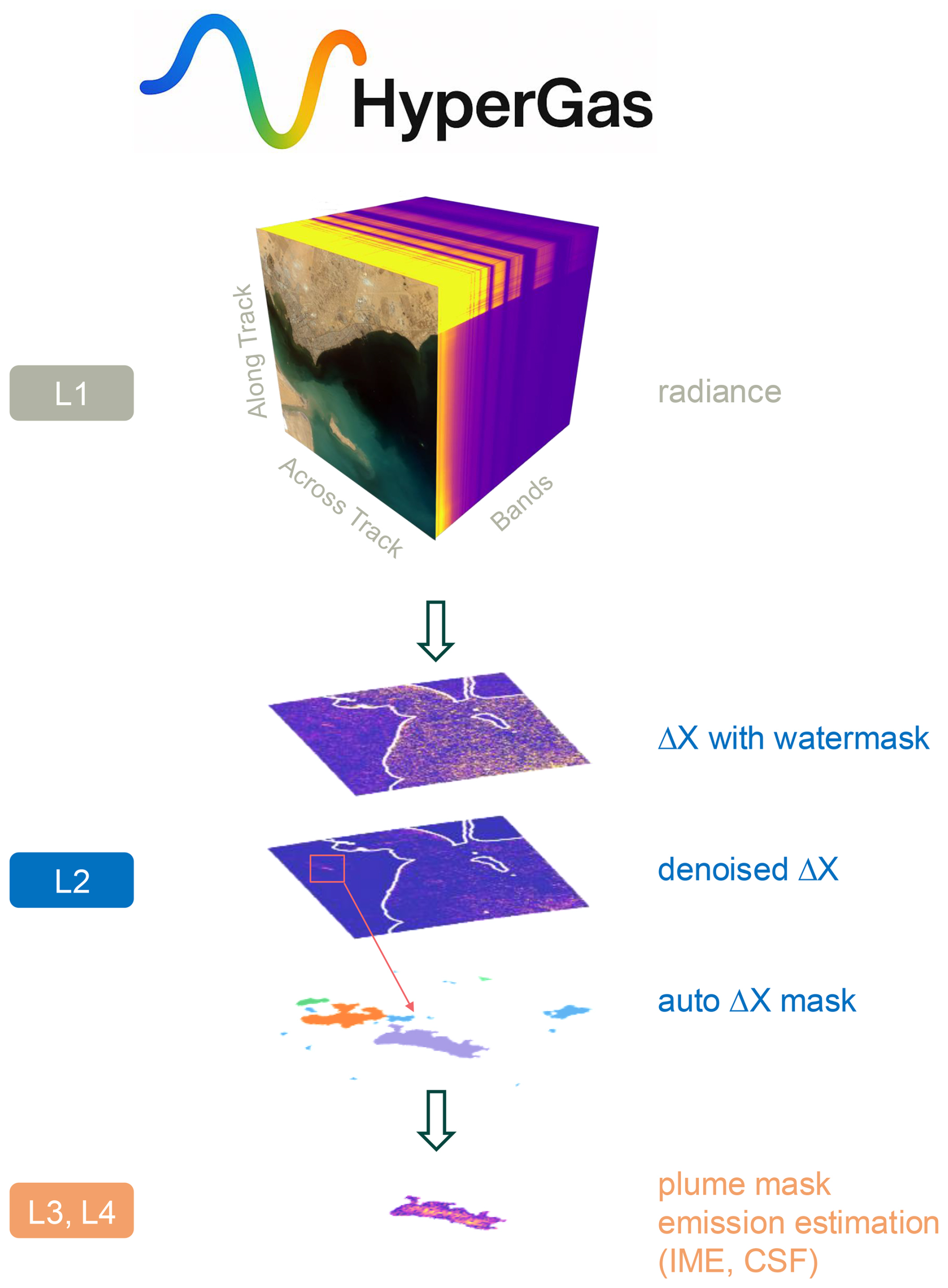
Figure 1 Workflow of the HyperGas package (L1–L4). The input consists of L1 calibrated radiance at sensor sampling. Greenhouse gas retrieval produces L2 concentration enhancements (ΔX), which are automatically denoised for plume detection and masking. The plume data (L3) is then used to estimate emissions (L4) with the integrated mass enhancement (IME) and cross-sectional flux (CSF) methods.

We describe the user interface in Sect. 2.5. The HyperGas framework supports a wide range of hyperspectral satellite data and aircraft observations, as long as they contain radiance data for retrieving greenhouse gases. For existing L2 data, the package can also be employed to only perform plume detection, segmentation, and emission estimation. Several additional data inputs are used in HyperGas. Due to the significant differences in surface albedo and thereby radiance levels over land and water (Funk et al., 2001; Foote et al., 2020), the retrieval process incorporates a water mask to separately process land and water pixels, as described in Sects. 2.1.2 and 2.2. Additionally, wind reanalysis data (Sect. 2.1.3) are essential for estimating greenhouse gas emission rates from plume imagery, as outlined in Sect. 2.4.

2.1 Data preparation

2.1.1 L1 radiance data

HyperGas v1.0 initially focuses on processing L1 radiance data from three HSIs (PRISMA, EnMAP, and EMIT) but can be expanded for other hyperspectral data products such as aircraft observations. These three instruments cover key absorption bands of methane (weak and strong absorption windows around 1700 and 2300 nm) and CO₂ (1928–2200 nm) within their relevant spectral ranges, enabling targeted gas detection (Foote et al., 2021). Table 1 provides a summary of key characteristics of the hyperspectral satellite instruments.

Table 1 Description of hyperspectral satellite instruments.

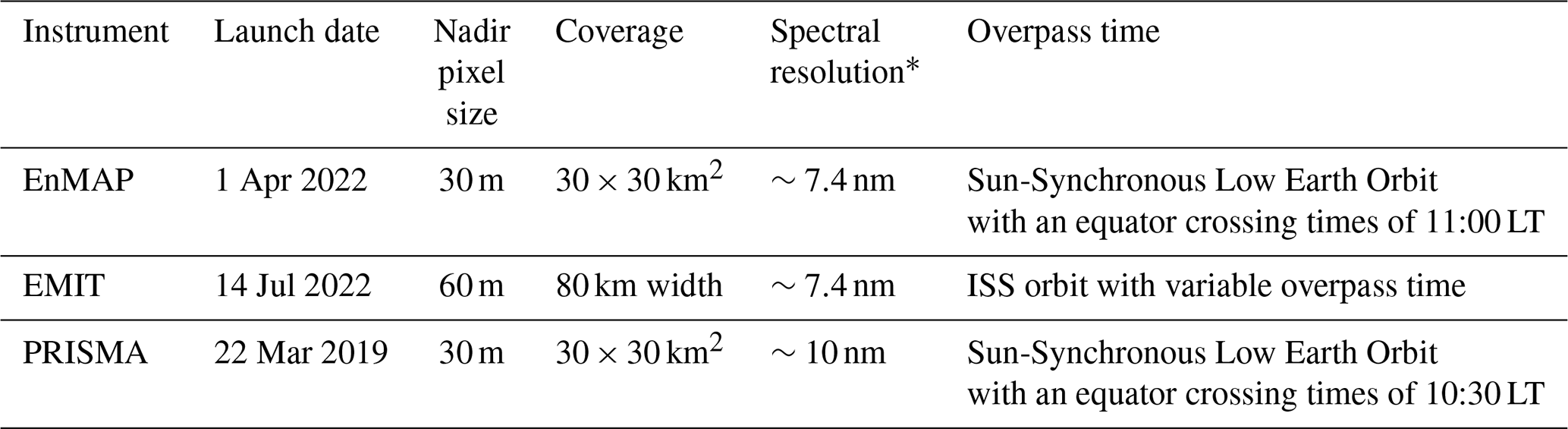
^* Typical average spectral resolution in the shortwave infrared (SWIR) range.

For PRISMA, the L1 data are obtained from the PRISMA Portal (Italian Space Agency, 2026); for EnMAP, these come from the EOWEB GeoPortal (DLR – German Aerospace Center, 2026); and for EMIT, users can download L1 data from NASA Earthdata (Green, 2022). Since no pre-treatment is applied to the L1 data, spectral calibration errors (e.g., central wavelength shifts and full-width at half-maximum variations) can propagate into retrievals due to the absorption structure of trace gases in the fitting window. Compared to PRISMA, sensors such as EnMAP have shown a smaller spectral smile, resulting in improved across-track uniformity (Roger et al., 2024; Ferrari et al., 2026). A potential mitigation strategy is to fit modeled spectra against reference spectra to correct for spectral calibration errors and improve retrieval accuracy (Guanter et al., 2021). This approach can be incorporated into HyperGas in future work. Because HSI file formats vary across different products, we have integrated multiple HSI readers into another Python package named Satpy (Raspaud et al., 2025), ensuring a standardized data loading interface that returns a three-dimensional data array (xarray.DataArray) organized as (bands, y, x), where the first dimension represents spectral bands and the remaining two represent spatial coordinates (Hoyer and Hamman, 2017). This makes it easy to support new HSI data.

PRISMA Level 1 data lacks geolocation details, such as rational polynomial coefficients (RPCs) or a geometric lookup table (LUT), which are typically used for precise image positioning, or georeferencing. Therefore, we manually correct the offset for L2–L4 products using Ground Control Points (GCPs) that are visually identified from distinct features on Earth's surface (e.g., road intersections), while RPCs and LUTs are applied for EnMAP and EMIT data, respectively.

2.1.2 Water mask

We classify pixels as land or water by using 10 m integrated data from both OpenStreetMap (OSM) and ESA WorldCover databases (Kennedy et al., 2024). ESA WorldCover data primarily encompass Canada, Alaska, and Russia, while OpenStreetMap data covers the remaining global regions. Both datasets are combined to create a global dataset. The implemented water mask identifies both coastal waters and major inland water bodies.

HyperGas also supports two other datasets available through the cartopy feature interface (Elson et al., 2024): the Global Self-consistent, Hierarchical, High-resolution Geography (GSHHG) database and the 10 m Natural Earth dataset. The water mask is used in the clustering of pixels to separately apply a retrieval for land and water pixels (Sect. 2.2.1). Figure 2 compares the water masks around the Caspian Sea as well as a K-means clustering approach that further disaggregates the scene (Sect. 2.2.1). The OSM and ESA WorldCover datasets effectively differentiate between land and water, whereas the GSHHG dataset misclassifies some sea areas as land, and the Natural Earth dataset omits inland water bodies. These differences in masking can lead to variations in retrieval results (see Sect. 2.2.1).

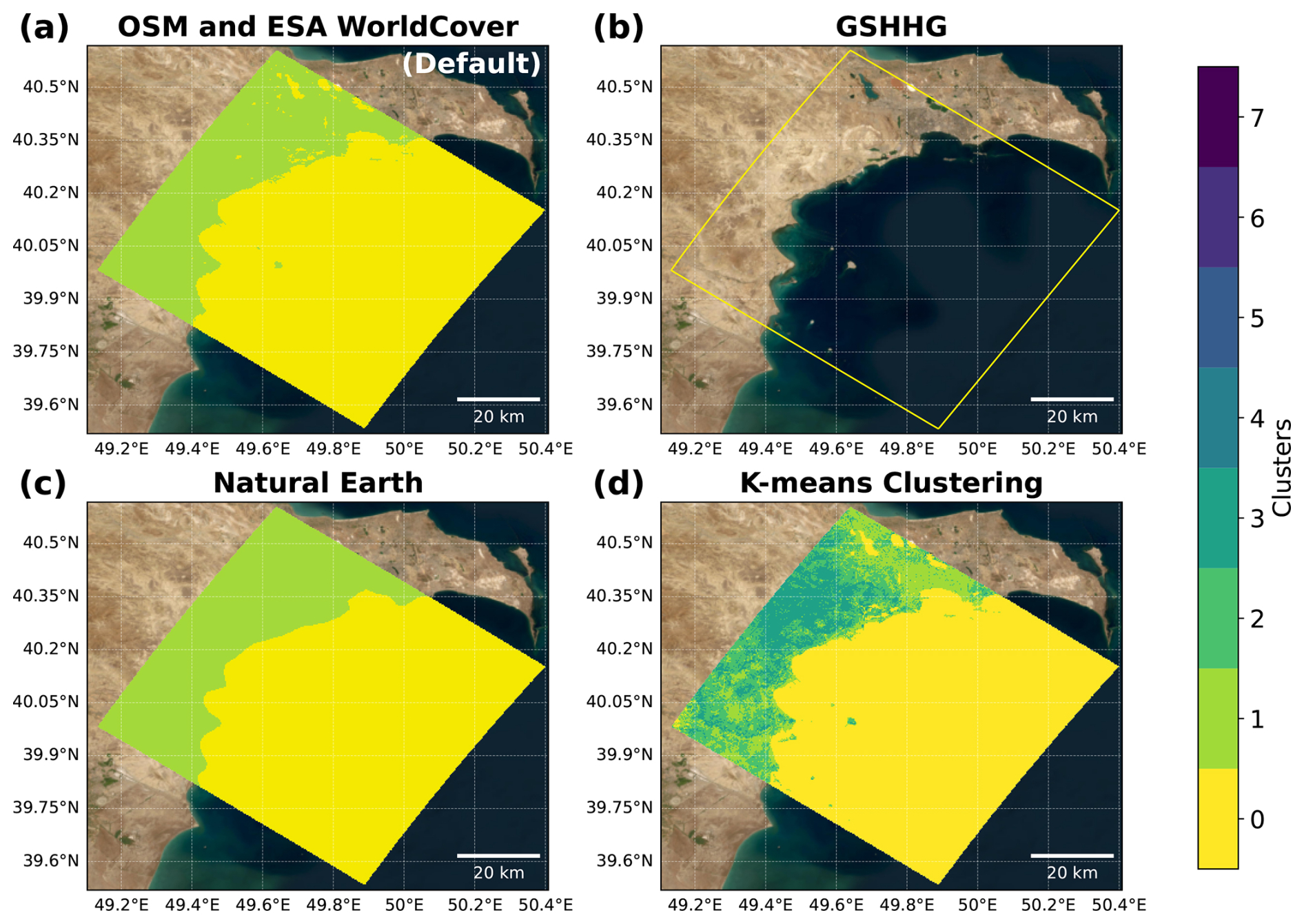
Figure 2 EMIT pixel clusters derived from (a) OpenStreetMap (OSM) and ESA WorldCover databases, (b) the Global Self-consistent, Hierarchical, High-resolution Geography database (GSHHG), (c) the Natural Earth dataset, and (d) k-means clustering. Water pixels are assigned a value of zero (yellow), while land pixels are assigned values greater than or equal to one, with specific classifications determined using the k-means clustering method. In the case of the GSHHG dataset, all pixels are classified as land but are shown as transparent with the EMIT scene outlined in yellow for comparison against the ESRI World Imagery. Source: Esri|Powered by Esri.

2.1.3 Wind data

Wind speed and direction control greenhouse gas transport in the atmosphere, thus they are important input data for plume determination and emission quantification. The default wind product used in the analysis is the European Centre for Medium-Range Weather Forecasts Reanalysis 5 (ERA5, 0.25°×0.25°) 10 m hourly wind data (Hersbach et al., 2020; Carver and Merose, 2023). The GEOS Forward Processing (GEOS-FP, 0.25° latitude × 0.3125° longitude) and Open-Meteo (Zippenfenig, 2023) 10 m wind data are also supported.

2.2 Greenhouse gas retrieval

2.2.1 Matched filter

To determine the amount of gas (e.g., methane or CO₂) above the background in the atmospheric column at a specific location, we apply a mathematical method known as the linear matched filter. This approach has been successfully applied to satellite and aircraft observations (Thompson et al., 2015; Foote et al., 2021; Thorpe et al., 2023; Roger et al., 2024). By default, we exclude water bands (1358–1453 and 1814–1961 nm) which can affect the retrieval of methane and CO₂. The modeled spectrum affected by the gas absorption (x_m) is defined according to the Beer–Lambert law:

$$\begin{array}{}\text{(1)}& {\mathit{x}}_{\mathrm{m}}={\mathit{x}}_{\mathrm{r}}{e}^{-\mathit{k}\mathrm{\Delta }X},\end{array}$$

where x_r is the reference spectrum and k is a unit absorption spectrum. The strong absorption windows of 2100–2450 nm for methane and 1930–2200 nm for CO₂ are selected for calculating the gas column enhancement (ΔX). The matched filter method treats the background spectral signature as a Gaussian distribution (𝒩) with a mean vector μ and covariance matrix Σ.

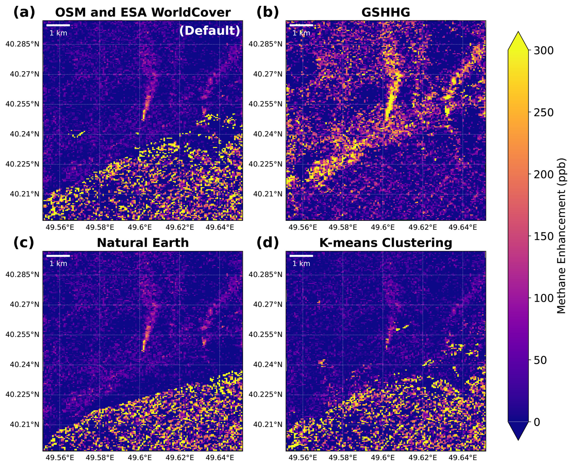
Figure 3 Retrieved methane enhancements from the EMIT observation over Azerbaijan on 21 April 2024, based on matched filter analysis applied to each pixel cluster as defined in Fig. 2.

The radiance spectrum (L) considers two scenarios: a null hypothesis H₀ representing background conditions, and an alternative hypothesis H₁ indicating the presence of enhanced gas concentrations (Thompson et al., 2015).

$$\begin{array}{}\text{(2)}& H_{\mathrm{0}}:L\sim \mathcal{N}(\mathit{\mu },\mathbf{\Sigma });H_{\mathrm{1}}:L\sim \mathcal{N}(\mathit{\mu }+\mathrm{\Delta }X\mathit{t},\mathbf{\Sigma })\end{array}$$

The target signature t is defined as the product of the background mean radiance (μ) and the negative gas absorption coefficient (k). To derive k, we apply a radiative transfer model (Gloudemans et al., 2008), incorporating the instrument's spectral response function characterized by its central wavelength and full width at half maximum (FWHM; Thompson et al., 2015). The atmosphere is divided into vertical layers with a thickness of 1 km up to an altitude of 25 km, 2.5 km between 25 and 50 km, and 5 km above 50 km altitude. We use the seasonal Air Force Geophysical Laboratory (AFGL) atmospheric constituent profiles and simulate various gas enhancement scenarios in the lowermost atmospheric layer (0–1 km) using the forward model. For methane, we evaluate enhancements from 0 to 6400 ppb in geometric progression (doubling from 100 ppb), while CO₂ enhancements range from 0 to 160 ppm (doubling from 2.5 ppm), reflecting the broader dynamic range and higher background concentration of CO₂ compared to methane. For airborne data, users can modify the configuration file to compute k in ppmm units. The k value for each band is determined through linear regression between the natural logarithm of the simulated radiance and gas enhancement values. The optimal estimate of the enhancement factor ΔX is obtained through maximum likelihood estimation:

$$\begin{array}{}\text{(3)}& \mathrm{\Delta }X={\displaystyle \frac{(\mathit{t}-\mathit{\mu }{)}^T{\mathbf{\Sigma }}^{-\mathrm{1}}(\mathit{L}-\mathit{\mu })}{(\mathit{t}-\mathit{\mu }{)}^T{\mathbf{\Sigma }}^{-\mathrm{1}}(\mathit{t}-\mathit{\mu })}}.\end{array}$$

Optical aberrations can cause variations in central wavelength and spectral resolution among detectors within the same array (Guanter et al., 2009), leading to non-uniformity across data-cube columns in the across-track direction. Therefore, the matched filter is implemented separately for each along-track column. We apply the matched filter to each cluster (Fig. 2) separately to account for differences in background signals (e.g., land versus water pixels). The algorithm is applied through the Spectral Python (SPy) package (Boggs et al., 2022), which supports the matched filter method. Figure 3 shows the retrieved methane enhancements ($\mathrm{\Delta }{X}_{{\mathrm{CH}}_{\mathrm{4}}}$) associated with methane leaks in Azerbaijan, derived using different water masks. The GSHHG mask, which treats all pixels as land, produces overestimated methane retrievals with higher noise levels (Fig. 3b). Results obtained with Natural Earth data are similar to those from the default OSM and ESA WorldCover masks, though Natural Earth fails to effectively differentiate inland/coastal water pixels (Fig. 3c).

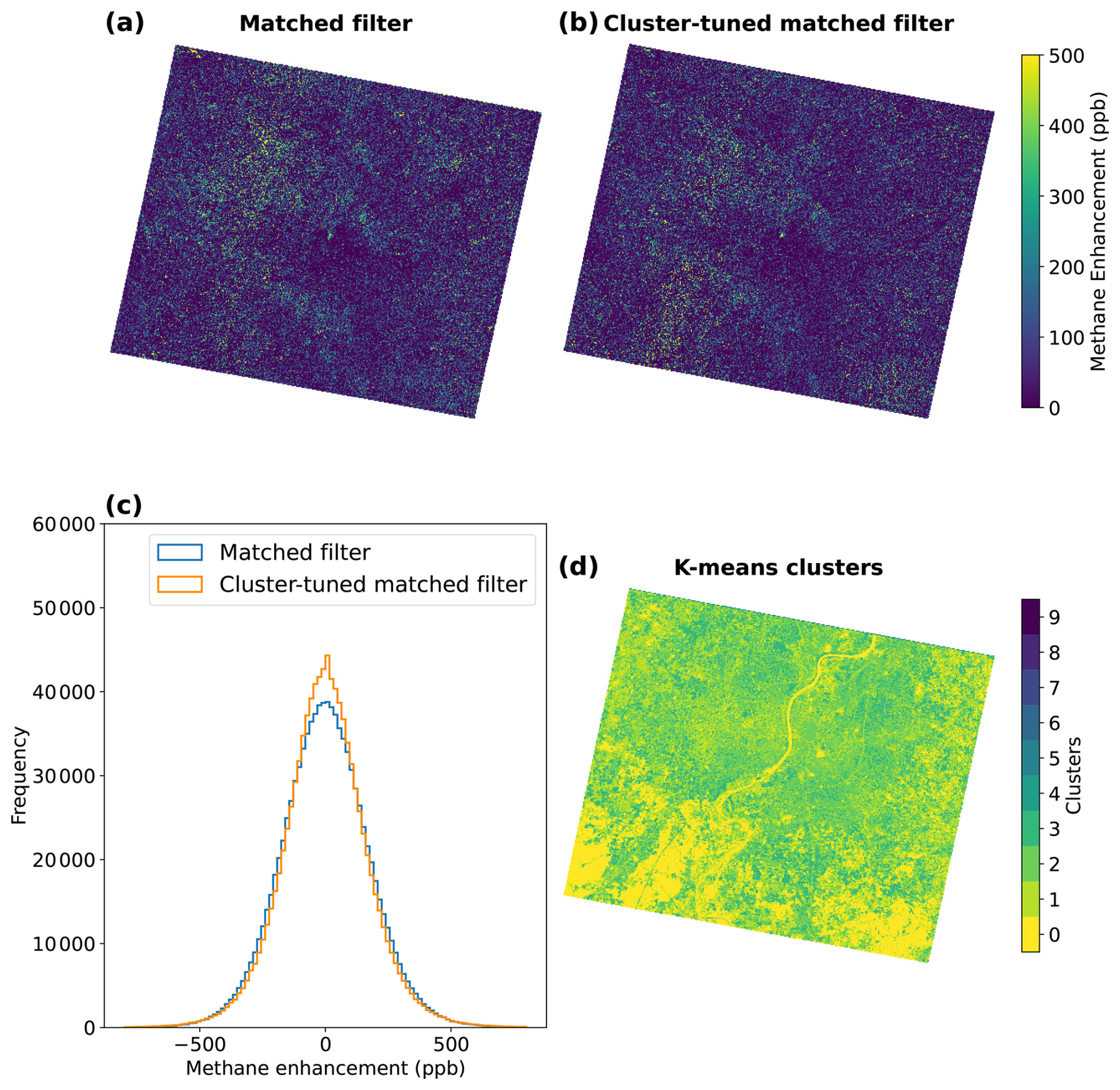
Previous studies on aircraft observations suggest that applying the matched filter to clustered pixels can reduce background noise such as the albedo effect caused by roads and building infrastructures (Funk et al., 2001; Thorpe et al., 2013). We first apply the principal component analysis (PCA) to reduce the dimension of the data space. Then we use the k-means algorithm to classify all pixels into clusters. Users can adjust the kmeans.nclusters argument to test the sensitivity (Funk et al., 2001). The k-means clustering approach tends to underestimate methane enhancements, presumably due to the reduced pixel count allocated to each cluster (Fig. 3d). We have also tested the cluster-tuned matched filter in urban areas (Fig. A1), however, the results are still noisy, making it challenging to differentiate plumes from the background. The improved retrieval performance of previous airborne imaging spectrometers is likely related to their higher spatial resolution (3–8 m) and narrower swath width (∼5 km) compared with HSIs, which also leads to longer observed plumes within a single scene. Another challenge in the cluster analysis is the cross-track variability, which includes the smile effect (Guanter et al., 2021), thereby affecting the cluster-tuned matched filter. A joint application of smile-effect correction and a cluster-tuned matched filter could improve retrieval performance and can be developed for HyperGas at a later stage. Therefore, HyperGas does not rely on the k-means method but instead applies land and water masks derived from the OSM and ESA WorldCover datasets.

2.2.2 Lognormal matched filter

One limitation of the matched filter is the linear approximation, which could lead to underestimated enhancements in large plumes (Schaum, 2021; Pei et al., 2023). Therefore, HyperGas provides the lognormal matched filter method which applies logarithms to both sides of Eq. (1):

$$\begin{array}{}\text{(4)}& \ln \left({\mathit{x}}_{\mathrm{m}}\right)=\ln \left({\mathit{x}}_{\mathrm{r}}\right)-\mathit{k}\mathrm{\Delta }X.\end{array}$$

This addresses the limitation of the first-order Taylor expansion, which assumes weak absorption that can be approximated as linear, whereas in regions of strong methane enhancement the absorption departs from this linear behavior. Then the optimal estimate of ΔX is derived as below:

$$\begin{array}{}\text{(5)}& \mathrm{\Delta }X={\displaystyle \frac{(\mathit{k}-\stackrel{\mathrm{̃}}{\mathit{\mu }}{)}^T{\stackrel{\mathrm{̃}}{\mathbf{\Sigma }}}^{-\mathrm{1}}(\stackrel{\mathrm{̃}}{\mathit{L}}-\stackrel{\mathrm{̃}}{\mathit{\mu }})}{(\mathit{k}-\stackrel{\mathrm{̃}}{\mathit{\mu }}{)}^T{\stackrel{\mathrm{̃}}{\mathbf{\Sigma }}}^{-\mathrm{1}}(\mathit{k}-\stackrel{\mathrm{̃}}{\mathit{\mu }})}},\end{array}$$

where $\stackrel{\mathrm{̃}}{\mathit{\mu }}$ is the mean log background radiance, $\stackrel{\mathrm{̃}}{\mathbf{\Sigma }}$ is the covariance matrix of the log background radiance, and $\stackrel{\mathrm{̃}}{\mathit{L}}$ is the log radiance spectrum. Figure 4 compares the results obtained using the matched filter and the lognormal matched filter. The methane enhancement differences can reach up to 50 ppb, potentially impacting subsequent emission rate quantification. Since measurement noise can produce negative radiance values in some spectral bands, the lognormal matched filter, which assumes strictly positive inputs, may amplify background noise. Therefore, HyperGas defaults to the standard matched filter and switches to the lognormal matched filter when strong methane enhancements are detected. Specifically, if more than five pixels within the plume mask exceed 1200 ppb, the data are reprocessed using the lognormal matched filter, following the sensitivity analysis in Pei et al. (2023). Because the CO₂ data are generally noisier than the methane data, HyperGas does not automatically switch to the lognormal matched filter for CO₂.

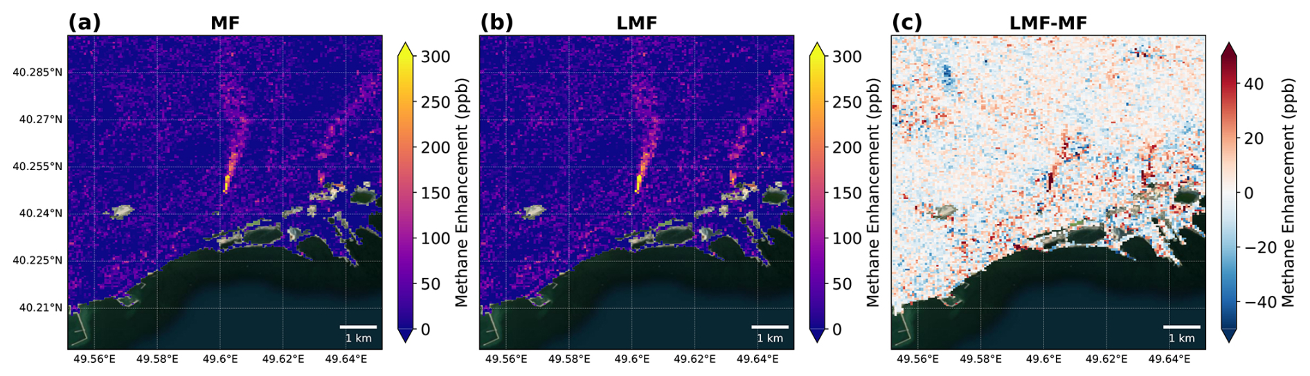
Figure 4 Retrieved methane enhancements from the EMIT observation over Azerbaijan on 21 April 2024, using (a) the matched filter method and (b) the lognormal matched filter method. Panel (c) shows the difference between the two retrievals. Water pixels are masked using the OSM and ESA WorldCover data sets. Background imagery source: Esri|Powered by Esri.

2.3 Plume detection

For plume detection, we perform the matched filter over the entire near-infrared window (1300–2500 nm, Roger et al., 2024), instead of only over the strong methane (2100–2450 nm) and CO₂ (1928–2200 nm) absorption windows, to mitigate the background noise in heterogeneous areas. This includes the additional methane absorption features around 1700 nm as well as additional background wavelengths without sensitivity to methane. Then, we apply a Chambolle total variation (TV) denoising filter (Chambolle, 2004) to reduce noise and obtain a smoother ΔX field. This technique reduces noise by minimizing the total variation of the image, which refers to the integral of the gradient magnitude, while preserving sharp features such as edges. Unlike traditional smoothing methods such as median filtering, TV denoising effectively suppresses noise while preserving meaningful structures, making it more suitable for retaining localized enhancements. Because different scenes detected by different instruments have different noise levels, we calibrate the denoisers for each scene and instrument using J-Invariance (Batson and Royer, 2019). The denoised ΔX field is only used for generating plume masks because of its differing magnitude, while the emission rate calculation relies on ΔX data retrieved from strong absorption windows without denoising. Figure 5a shows an example of the denoised $\mathrm{\Delta }{X}_{{\mathrm{CH}}_{\mathrm{4}}}$ field for the scene from Fig. 3a.

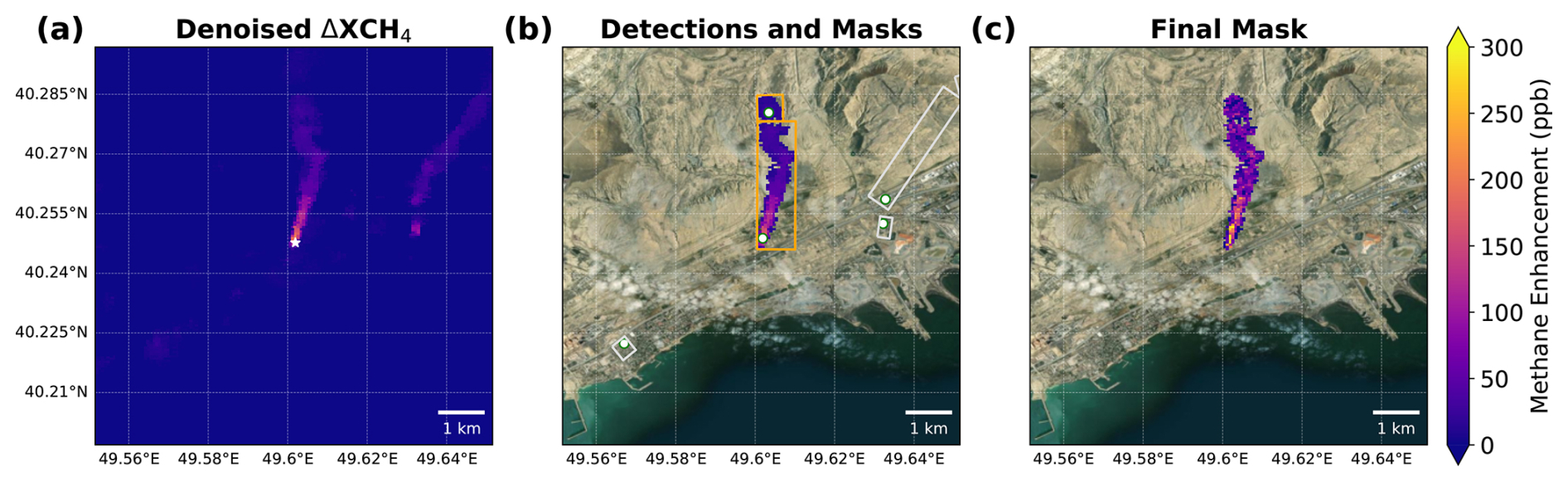
Figure 5 Plume mask creation process for the western plume from Fig. 3a. (a) The denoised methane enhancement ($\mathrm{\Delta }{X}_{{\mathrm{CH}}_{\mathrm{4}}}$) field obtained by applying the Chambolle total variation (TV) denoising filter to $\mathrm{\Delta }{X}_{{\mathrm{CH}}_{\mathrm{4}}}$ within the 1300–2500 nm window. The white star marks the manually identified source location for the western plume. (b) Initial candidate masks derived from the watershed algorithm. White dots indicate high-$\mathrm{\Delta }{X}_{{\mathrm{CH}}_{\mathrm{4}}}$ locations, and colored rectangles represent the minimum rotated rectangles (oriented bounding boxes) for each mask. Orange rectangles denote masks with azimuth differences less than 30° relative to the reference mask (containing the source marker of the western source) and are merged into a single plume. The gray rectangles are candidates excluded by the azimuth criterion. (c) The final $\mathrm{\Delta }{X}_{{\mathrm{CH}}_{\mathrm{4}}}$ plume mask for the western emission source after merging. Background imagery source: Esri|Powered by Esri.

We derive gas plume masks using a semi-supervised method that starts by applying a watershed technique to the denoised fields (Fig. 5b) with the tobac Python package. This method has been applied to track convective clouds (Heikenfeld et al., 2019), NO₂ plumes in TROPOMI observations (Zhang et al., 2023), and methane plumes in hyperspectral observations (Zhang et al., 2025). It treats pixel values as a topographic surface and separates them into different basins. We use a threshold of two standard deviations (2σ) above the mean to identify localized high-enhancement features. We then use a threshold of 3σ to further separate features that were connected using the lower threshold (Fig. 5b; Rast et al., 2021). Once features are determined, the watershed expands outward from the features until it reaches the lower threshold (2σ). We dilate these masks by 180 m and merge overlapping masks.

Emission sources are manually identified based on wind data and ESRI imagery. To determine whether multiple candidate masks belong to the same emission source, we calculate the minimum rotated rectangle (oriented bounding box) for each mask. The mask containing the manually identified source is designated as the reference, and we compute the azimuth difference between its rectangle and those of all other candidates. Only masks with azimuth differences less than 30° relative to the reference are merged together as a single plume (e.g., orange rectangles in Fig. 5b), assuming minimal wind direction changes near the source. This azimuth-based filtering helps exclude spurious detections or plumes from different sources (e.g., gray rectangles in Fig. 5b). Figure 5c demonstrates the final mask determined for the western methane emission plume in the scene.

If a plume is truncated or improperly segmented, HyperGas allows users to adjust the dilation distance and azimuth threshold to obtain a more appropriate plume mask (e.g., for the eastern plume in Fig. 5a). Non-detects are classified when no plume mask is detected near the source of interest. Users can inspect the masked plumes through the graphical user interface (Sect. 2.5.2) to evaluate correlation with additional data fields such as albedo and RGB imagery to ensure the identified plume is not an artifact (e.g., smoke).

2.4 Emission estimation

Since the matched filter assumes plume signals are sparse (i.e., present in only a small fraction of pixels), we exclude pixels within identified plume masks when computing μ and Σ, so that background statistics are estimated only from non-plume pixels and the sparsity assumption remains valid. The retrieval is then rerun to generate the final emission rate products. This two-step reprocessing approach reduces bias in background radiance estimates and typically yields higher methane emission rates.

Two widely used methods for estimating source emission rates from plume observations are the integrated mass enhancement (IME) method (Varon et al., 2018), which relates the total plume mass enhancement to the emission rate through a wind-speed-dependent parameterization, and the cross-sectional flux (CSF) method (Varon et al., 2018; Kuhlmann et al., 2024), which estimates the source rate as the product of methane enhancement and wind speed integrated across the plume width perpendicular to the wind direction. Both methods are available in HyperGas and described below, including the calibration of the required effective wind speed.

2.4.1 Estimation methods

We apply the IME method as the default method to estimate gas emission rates (Q in kg h⁻¹):

$$\begin{array}{}\text{(6)}& Q={\displaystyle \frac{\mathrm{IME}\cdot U_{\mathrm{eff},\mathrm{IME}}}{L}},\end{array}$$

where IME is the total gas mass enhancement (kg) within the plume mask, L (m) is the square root of the plume area, and U_eff,IME is the effective wind speed (m s⁻¹). The total gas mass enhancement is calculated by summing the product of the column mass enhancement (ΔΩ, kg m⁻²) and the area of each pixel (m²). The column mass enhancement ΔΩ is derived from ΔX:

$$\begin{array}{}\text{(7)}& \mathrm{\Delta }\mathrm{\Omega }={\displaystyle \frac{M_X}{M_{\mathrm{a}}}}{\mathrm{\Omega }}_{\mathrm{a}}\mathrm{\Delta }X,\end{array}$$

where M_X and M_a are the molar masses (kg mol⁻¹) of gas X and dry air ($\mathrm{28.96}\times {\mathrm{10}}^{-\mathrm{3}}$ kg mol⁻¹), and Ω_a is the column of dry air (kg m⁻²). Ω_a is defined as the ratio of surface pressure, obtained from GEOS-FP, ERA5, or Open-Meteo reanalysis data, to the acceleration of gravity.

In addition to the IME method using the full plume mask, HyperGas supports IME estimates with maximum fetch limits (IME-limit), which are particularly useful for characterizing elongated plumes (Duren et al., 2019; Thorpe et al., 2023; Duren et al., 2025).

Another method to calculate the emission rate is the CSF method. This method is especially useful if gaps in the detected plume, for example, caused by low albedo, make the estimate based on the total IME less reliable. Here, the source rate is estimated as the product of the cross-plume gas enhancement integral and a different effective wind speed (U_eff,CSF):

$$\begin{array}{}\text{(8)}& Q=U_{\mathrm{eff},\mathrm{CSF}}\underset{a}{\overset{b}{\int }}\mathrm{\Delta }\mathrm{\Omega }(x,y)\mathrm{d}y.\end{array}$$

Here, the x axis aligns with the wind direction, while the y axis is oriented perpendicular to it. The integral is evaluated between the plume boundaries [a, b], as defined by the cross section in the plume mask. The centerline is defined by fitting a weighted cubic polynomial through the plume enhancement field, where weights correspond to gas enhancements. Fitting is performed in a coordinate system rotated to align with the principal plume direction (source to enhancement-weighted centroid), with ridge regularization (α=0.1) to ensure smooth solutions. This plume-aligned cubic fit improves the quadratic method in ddeq (Kuhlmann et al., 2024) by better capturing plume curvature. Cross-sectional lines are positioned at equal arc-length intervals along the centerline. Each line is oriented perpendicular to the local centerline tangent where it intersects the plume mask. The spacing between CSF sections is set to 2.5× pixel resolution, rather than 1× pixel resolution, to reduce overlap between adjacent sections and ensure sufficient independence of sampled data.

2.4.2 Wind calibrations

For both the IME and CSF, an effective wind speed is required, which needs to be related to the model's wind speed parameters. To calibrate U_eff,IME and U_eff,CSF against the domain-averaged 10 m wind speeds (U₁₀), we have used five 3 h large-eddy simulations (LES) performed using the Weather Research and Forecasting model (WRF-LES) at 25 m spatial resolution and 30 s temporal resolution (Varon et al., 2018; Maasakkers et al., 2022). The simulation accounts for varying meteorological conditions, including a range of mixed layer depths (500–2000 m) and sensible heat fluxes (100–300 W m⁻²), representing typical conditions observed with SWIR satellite instruments. Moreover, as the LES-based wind calibrations are derived using simulations over land, specific offshore calibrations could be added in the future to improve results for plumes over water such as from offshore oil and gas platforms. To match sensor spatial resolution, the WRF-LES data are conservatively resampled to 30 m for EnMAP and PRISMA and to 60 m for EMIT. The resampling weights are based on the ratio of source cell area overlapped with the corresponding destination cell. Simulations are conducted for two source types: a point source (e.g., oil and gas leaks or underground coal mine ventilation shafts; Sadavarte et al., 2021) and a 275×275 m² area source (e.g., landfills; Maasakkers et al., 2022). Emission rates are randomly scaled from 1–30 t h⁻¹ for methane (Zhang et al., 2025) and 0.5–3 kt h⁻¹ for CO₂ (Cusworth et al., 2023). The first simulation hour is used for turbulence spin-up, and the last 2 h are used in the wind calibration.

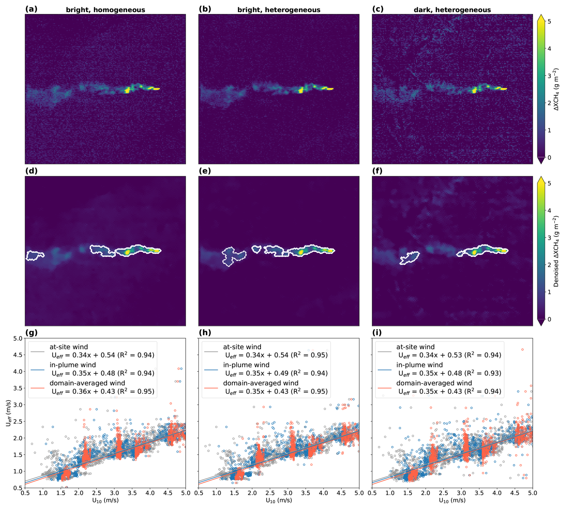
Figure 6 (a–c) Methane enhancement fields from point-source large eddy simulations over three EMIT scenes: bright and homogeneous, bright and heterogeneous, and dark and heterogeneous. (d–f) Corresponding denoised methane fields for the scenes shown in (a)–(c), with plume mask outlines shown in white. (g–i) Wind calibration results using three wind speed samplings: at-site values, in-plume estimates, and domain-averaged values.

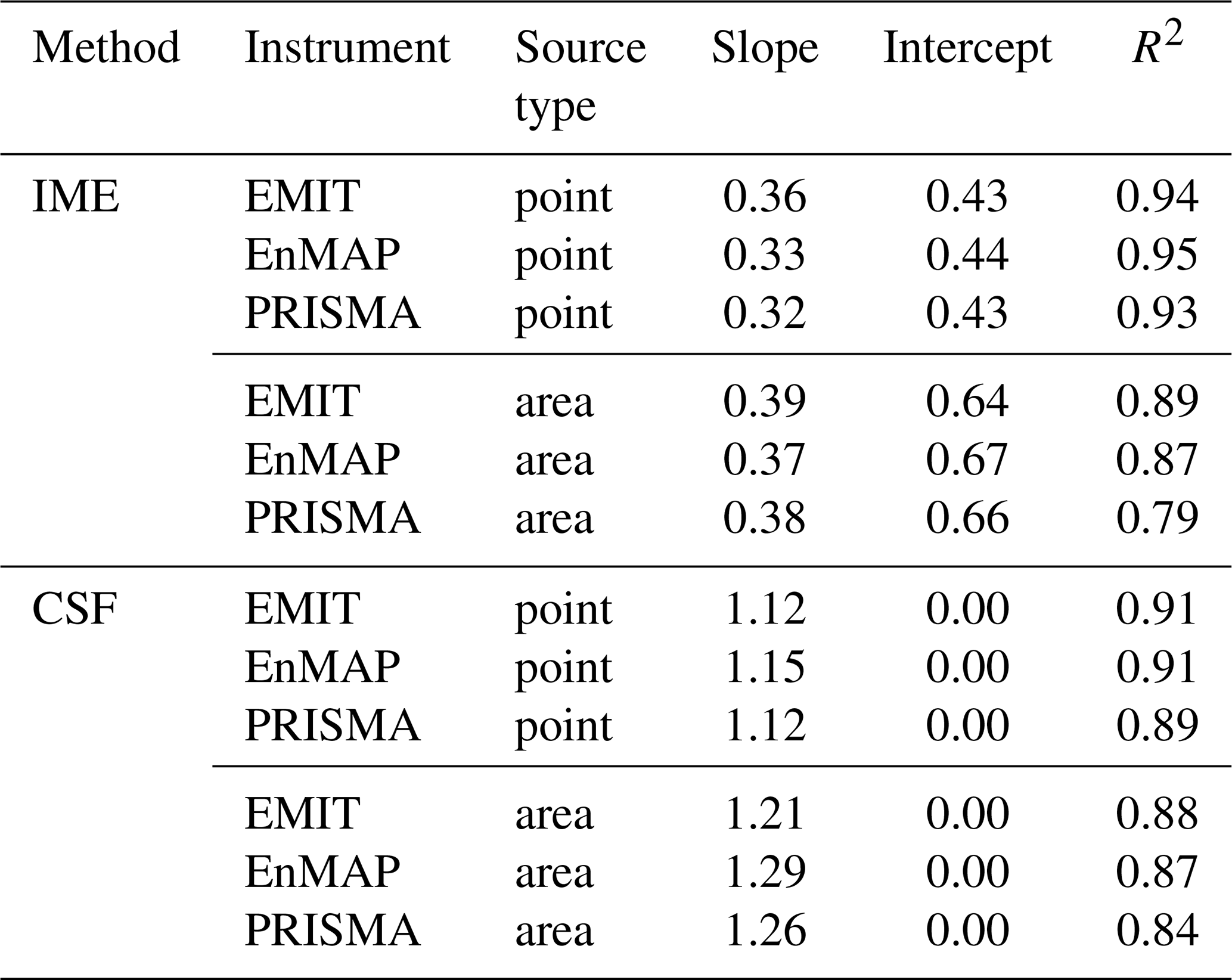
To incorporate realistic backgrounds, we overlay LES plumes onto cropped measured L2 scenes free of detected gas plumes for each imager. Backgrounds are drawn from three representative surface types: bright and homogeneous (Xinjiang, China), bright and heterogeneous (Anna Creek, Australia), and dark and heterogeneous (Madrid, Spain). For each simulated plume, U_eff,IME is computed as QL/IME, where Q is known, and L/IME is calculated from the plume mask. Despite differences in background complexity, the denoising step enables robust plume detection (Fig. 6d–f), and calibration coefficients are consistent across scenes (Fig. 6g–i). We therefore combine all 3600 cases to derive final calibration parameters for methane and CO₂ (Tables 2 and 3).

Table 2 Wind calibration settings used by default in the IME and CSF methods for methane, based on domain-averaged wind fields.

Table 3 Similar to Table 2 but for CO₂.

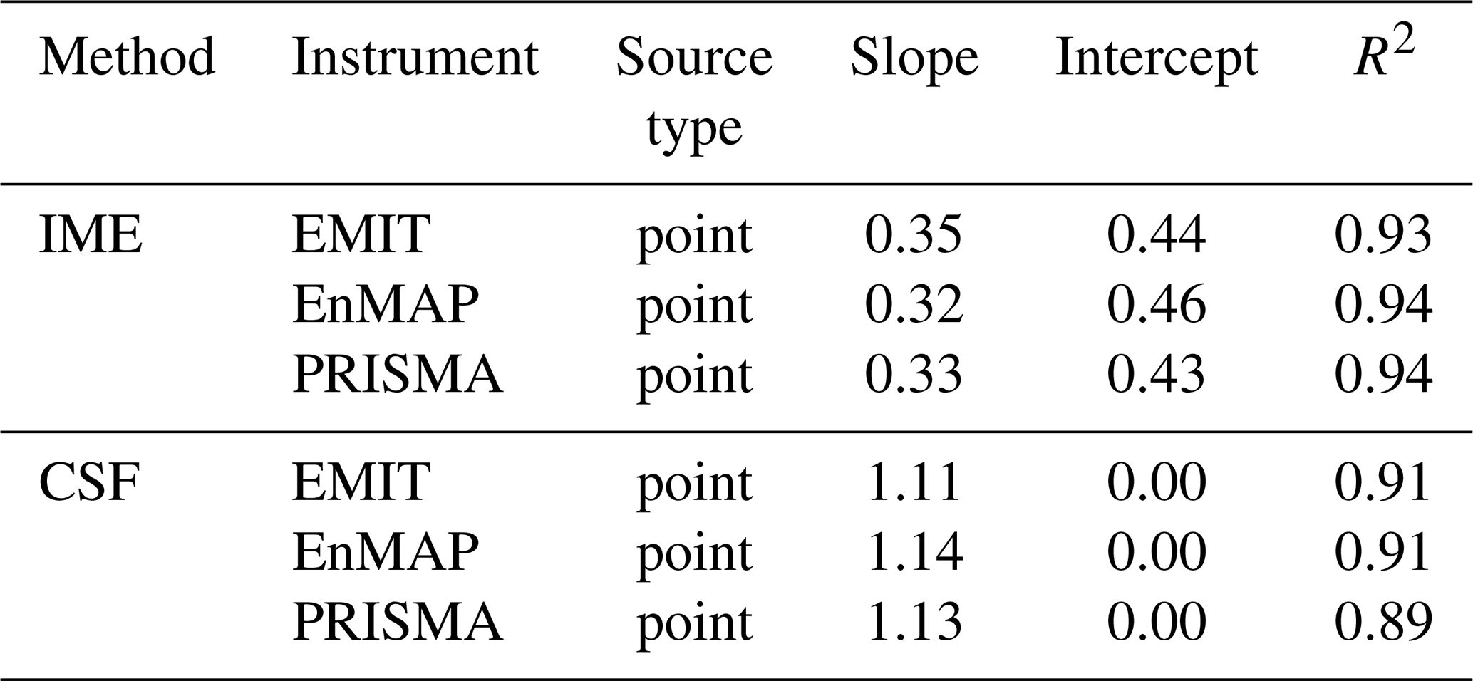
We evaluate the mean magnitude of U₁₀ from three LES-derived wind products for the wind calibration: at-site, in-plume, and 6×6 km² domain-averaged. At-site wind calibration is suitable for controlled releases with co-located wind measurements (Sherwin et al., 2023, 2024), whereas in-plume and domain-averaged products are better suited for applications relying on reanalysis wind speed data. Figure 6g–i shows that calibration results are similar across the three wind products. Accordingly, HyperGas defaults to the domain-averaged calibration for typical use cases involving reanalysis winds. While HyperGas allows users to input custom wind speeds, they must adjust the calibration settings in the configuration file to match their inputs if those products have different characteristics than the ones used here.

2.4.3 Emission uncertainty quantification

Our estimation of emission uncertainty for both the IME and CSF method accounts for four sources of uncertainty: wind speed error, retrieval random error, plume masking error, and wind calibration uncertainty (Varon et al., 2019, 2020; Maasakkers et al., 2022).

Wind speed error is quantified by applying a relative error of 50 % for wind speeds below 3 m s⁻¹ and a fixed error of 1.5 m s⁻¹ for wind speeds exceeding 3 m s⁻¹ (Varon et al., 2018; Zhang et al., 2025). To evaluate retrieval random error, we apply the same plume mask shape to non-plume areas across the scene, avoiding any overlap with the original plume location, and then calculate the standard deviation of the resulting emission rates (Varon et al., 2019; Zhang et al., 2025).

The plume masking procedure depends on two factors, the TV filter weight and watershed segmentation thresholds. For the TV filter weight, we examined two additional settings, 0.75 times and 1.5 times the default optimized value, alongside the baseline configuration. The default watershed thresholds are defined as mean + 2σ and mean + 3σ. In addition, we tested two alternative configurations, [mean + 1.5σ, mean + 2.5σ] and [mean + 2.5σ, mean + 3.5σ]. For each plume, we generated an ensemble comprising all parameter combinations and quantified the associated uncertainty as the standard deviation across the 9 ensemble members. The resulting mean relative emission uncertainties attributable to parameter selection are 8 %, 10 %, and 15 % for EMIT, EnMAP, and PRISMA, respectively.

Wind calibration error is the final source of uncertainty in our estimation. For point sources, the average U_eff fit residual is incorporated by adding it to the fitted U_eff equation, so that the fitting’s typical deviation is propagated into the uncertainty calculation. The area-source calibration method assumes a uniform methane emission distribution over a 275×275 m² region, even though actual emission patterns may be more complex (Maasakkers et al., 2022). To evaluate the uncertainty associated with this assumption, we apply the point-source calibration instead and examine the resulting variations in emission rates. The total uncertainty is defined as the square root of the sum of the squares of the individual uncertainties.

2.4.4 Plume fetch limits and controlled releases

Figure 7 shows wind calibrations for the IME and CSF methods across different plume length limits. Since Carbon Mapper applies a 2.5 km fetch limit (Duren et al., 2025), We have performed a sensitivity test using two thresholds: 1 and 2.5 km. The IME method with a 1 km plume limit has a significantly higher calibration slope compared to other configurations (Fig. 7a–c). The response of calibration slopes to decreasing fetch limits differs between the IME and CSF methods (Fig. 7d–f). This divergence reflects fundamental differences in methodology: restricting the fetch limit to 1 km reduces the number of plume pixels available for integration in the IME method, resulting in lower emission estimates when the shortened plume length cannot compensate for the reduced total gas mass enhancement. Conversely, the CSF method, which relies on cross-sectional measurements, may not sample broadly enough to produce a representative emission rate. Then, we split the final two hours of simulation data into calibration and validation subsets to assess whether applying fetch limits would improve performance during validation. However, the slopes between the true emission rates and the calibrated estimates remained approximately 1 across all fetch limits, indicating no improvement.

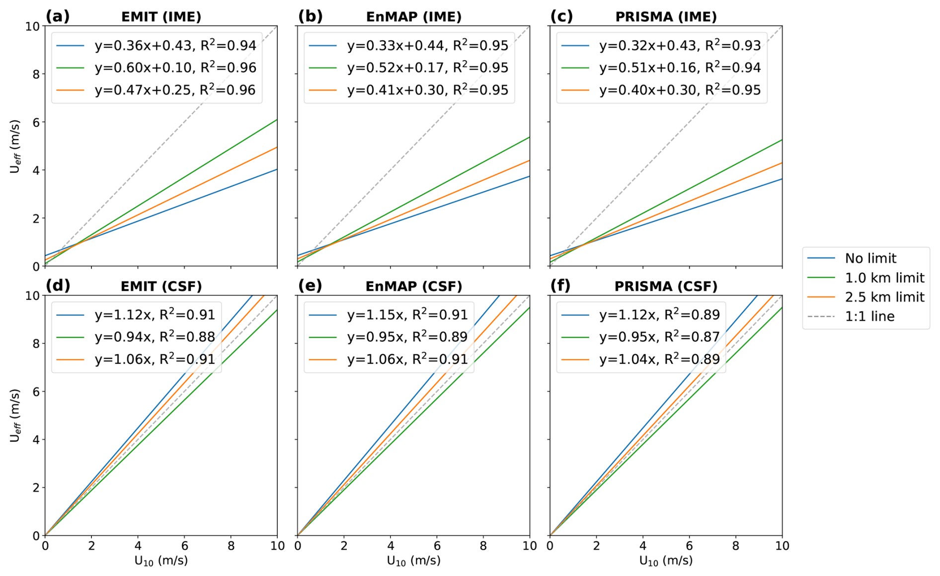
Figure 7 (a–c) Point-source IME calibrations for EMIT, EnMAP, and PRISMA. Colors indicate different fetch limits. (d–f) Same as (a)–(c), but using the CSF method.

We also validated our default IME and CSF estimates using 75 Stanford controlled releases conducted in 2024 and 2025 (Reuland et al., 2025; Brandt et al., 2026). The results show good agreement between the IME estimates and the controlled releases, with slopes ranging from 0.92 to 1.22 (Fig. 8). Since all plume lengths were under 1 km, any differences between the IME and IME fetch estimates are purely caused by different wind calibration coefficients and not by different sampling of the plumes. Figure 8 shows that the results do not differ significantly across the various IME fetch limits. HyperGas currently defaults to wind calibration without any fetch limitation.

Because short plume lengths may be insufficient for reliable CSF estimation, we perform CSF validation only for plumes with more than five CSF cross-section lines. The fitted slope between estimates and controlled release rates decreases from 1.47 to 1.16 when wind calibration is based on LES cases with emission rates below 2 t h⁻¹, while it remains unchanged for the IME method. Thus, we recommend using IME results by default and relying on CSF primarily for sensitivity analysis of the estimates. In the future, controlled release experiments involving elongated plumes may support calibration in two key ways: (1) evaluating the accuracy of different fetch limits, and (2) enabling wind calibration directly using measured U₁₀ data, which can then be applied to other cases with available wind observations.

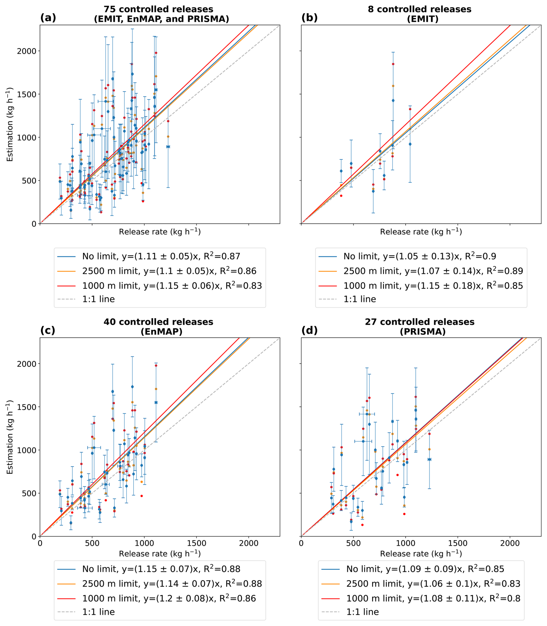
Figure 8 Quantification performance of methane‐emission estimates using the IME method under different fetch limits (none, 2500, and 1000 m) with calibrations shown in Fig. 7a–c. (a) Controlled releases observed by EMIT, EnMAP, and PRISMA. (b) EMIT only. (c) EnMAP only. (d) PRISMA only. Regression lines are fitted with Ordinary Least Squares (OLS). Estimation errors are derived from HyperGas outputs. The release‐rate errors are estimated as the standard deviation of mean emission rates released over consecutive time windows starting 1–5 min before and ending at the overpass time (i.e., [T−1 min, T], [T−2 min, T], …, [T−5 min, T]). For clarity, scatter points for the fetch-limited results are shown without error bars.

2.5 User interface

In addition to accessing functions via the Python API, HyperGas users can use Python batch processing scripts and an interactive application to efficiently process data from L1 to L4.

2.5.1 Batch processing

The general data processing workflow is outlined below:

• l2b_process.py and l2b_plot.py: generate L2 products, visualizations, and a summary HTML file that lets users compare different scenes by toggling layers.

• App: add plume markers interactively using the graphical user interface (see Sect. 2.5.2).

• l3b_process.py: produce L3 and L4 products, figures, and HTML files. This step can also be performed within the app.

• (optional) l2b_reprocess.py and l3b_reprocess.py: rerun the retrieval and emission rate estimates by excluding the plume pixels from each column of observations.

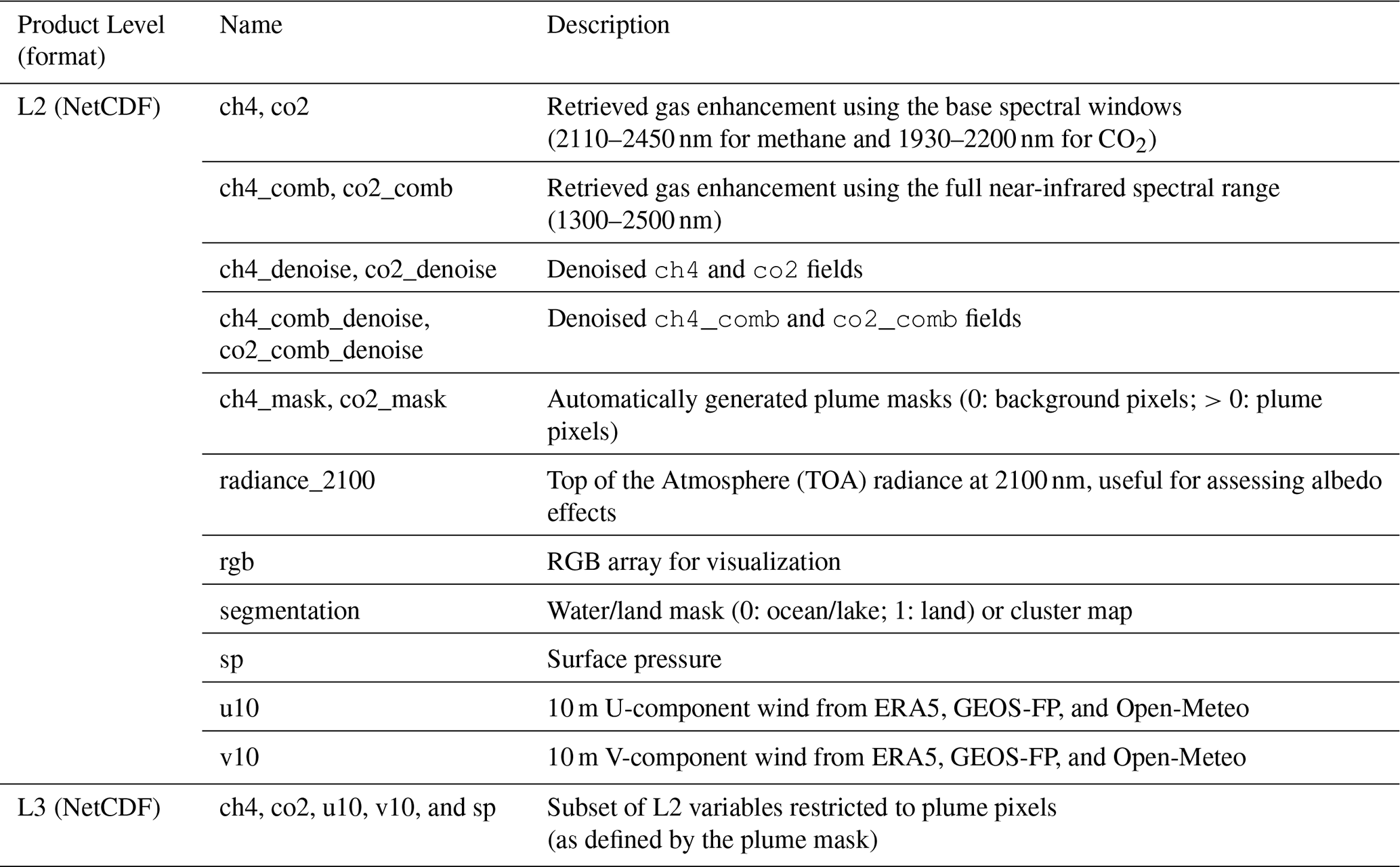
The variables included in the L2–L3 products are listed in Table B1. The L4 CSV file contains key plume-level information, including location, overpass time, wind conditions sampled from reanalysis products at the source location, emission rate and associated uncertainty, IME/CSF metrics, and additional details (For a full description, see the HyperGas User Guide: https://hypergas.readthedocs.io/, last access: 22 June 2026).

2.5.2 Interactive app

The emission rate calculation process begins with identifying plume source locations using HTML files generated by the script l2b_plot.py. This script embeds multiple L2B figures into a single HTML file, including key visualizations such as albedo, raw and denoised gas retrievals, plume masks, and wind vectors. By default, the interface displays only the denoised gas field for each observation group, allowing direct comparison of plume characteristics, especially changes in plume direction due to wind across different observation days. Users can then interactively add plume markers through a Streamlit-based web application that dynamically renders HTML content and executes embedded Python code. Because plume source locations may differ between observations, users must place markers individually for each L2B file. The selected marker positions are saved in the GeoJSON format to ensure accurate spatial referencing.

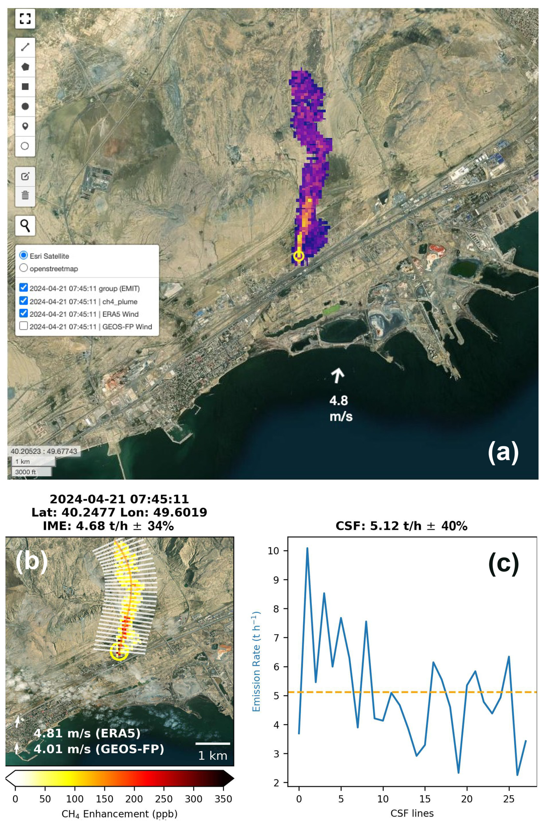
Figure 9 Example overview from the interactive application. (a) Methane plume overlaid on an ESRI basemap. Source: Esri|Powered by Esri. The emission source is marked with a yellow circle. Wind direction and speed based on ERA5 are indicated by the white arrow and text. (b) Overview of IME results. The title displays the satellite overpass time, source location, estimated emission rate, and associated uncertainty. Wind data from ERA5 and GEOS-FP are also shown. Background imagery source: Esri|Powered by Esri. (c) Emission rates along individual CSF lines, shown in white in panel (b). The mean CSF emission rate and uncertainty are shown in the title.

Once all marker files are ready, the l3b_process.py script automatically generates plume-level NetCDF files and computes emission rates for all cases. For a more streamlined and case-specific workflow, users can use the “Emission” page of the application, which provides a customizable interface for entering relevant parameters, such as site name, sector, wind speed, and surface pressure. Upon submission, the app generates a comprehensive output, displaying the final plume visualization and a corresponding L4 summary table on the same page (Fig. 9).

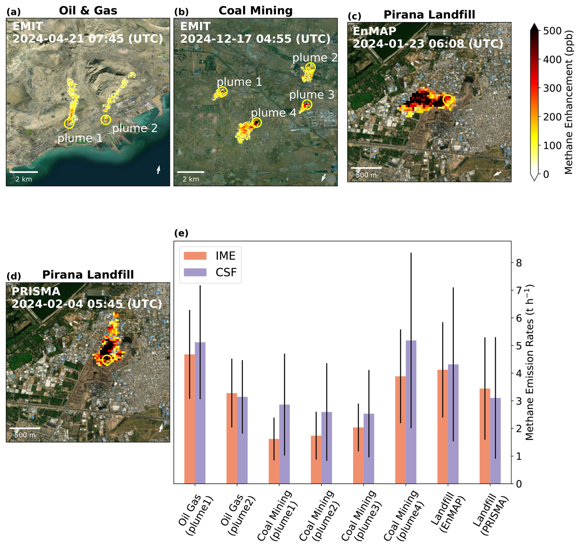
Figure 10 Methane plumes detected from various sectors using (a, b) EMIT, (c) EnMAP, and (d) PRISMA. Instrument and satellite overpass time are shown in white text at the top of each panel. Plume source locations are marked by yellow circles, with plume numbers annotated when multiple plumes are present in a single panel. ERA5 wind direction is indicated in the lower right corner of each image. (e) Methane emission estimates for the cases, derived using the IME and CSF methods. Background imagery source: Esri|Powered by Esri.

3 Applications

HyperGas currently supports the detection, retrieval, and quantification of methane and CO₂ plume emissions across various sectors. In the following sections, we present several examples of methane and CO₂ plumes observed in different contexts.

3.1 Methane emissions

Figure 10 shows methane plumes from three sectors: oil and gas operations (Baku, Azerbaijan), coal mining (Shanxi, China), and solid waste management (Pirana landfill, Gujarat, India). Figure 10a and b presents multiple plumes captured in a single observation, while Fig. 10c and d shows plumes from the same landfill site detected by both EnMAP and PRISMA. All plumes follow the ERA5 wind directions, while the source locations are either near the facilities or the deposited waste. In the case of the second oil and gas plume, the plume is truncated due to the dark surface and shows a curved shape. This required manual adjustments to the plume detection settings, specifically increasing the azimuth difference threshold from 30 to 60°.

Figure 10e compares the IME and CSF estimates for the four cases. While the average CSF estimates tend to be higher, particularly for short plumes, both methods are consistent within their respective uncertainty ranges. The agreement between EnMAP and PRISMA measurements at the Pirana landfill indicates that multiple hyperspectral satellite datasets can be effectively integrated to analyze temporal patterns in landfill methane emissions, as previously described by Zhang et al. (2025). These findings highlight the potential for hyperspectral remote sensing to contribute to global methane monitoring and mitigation efforts.

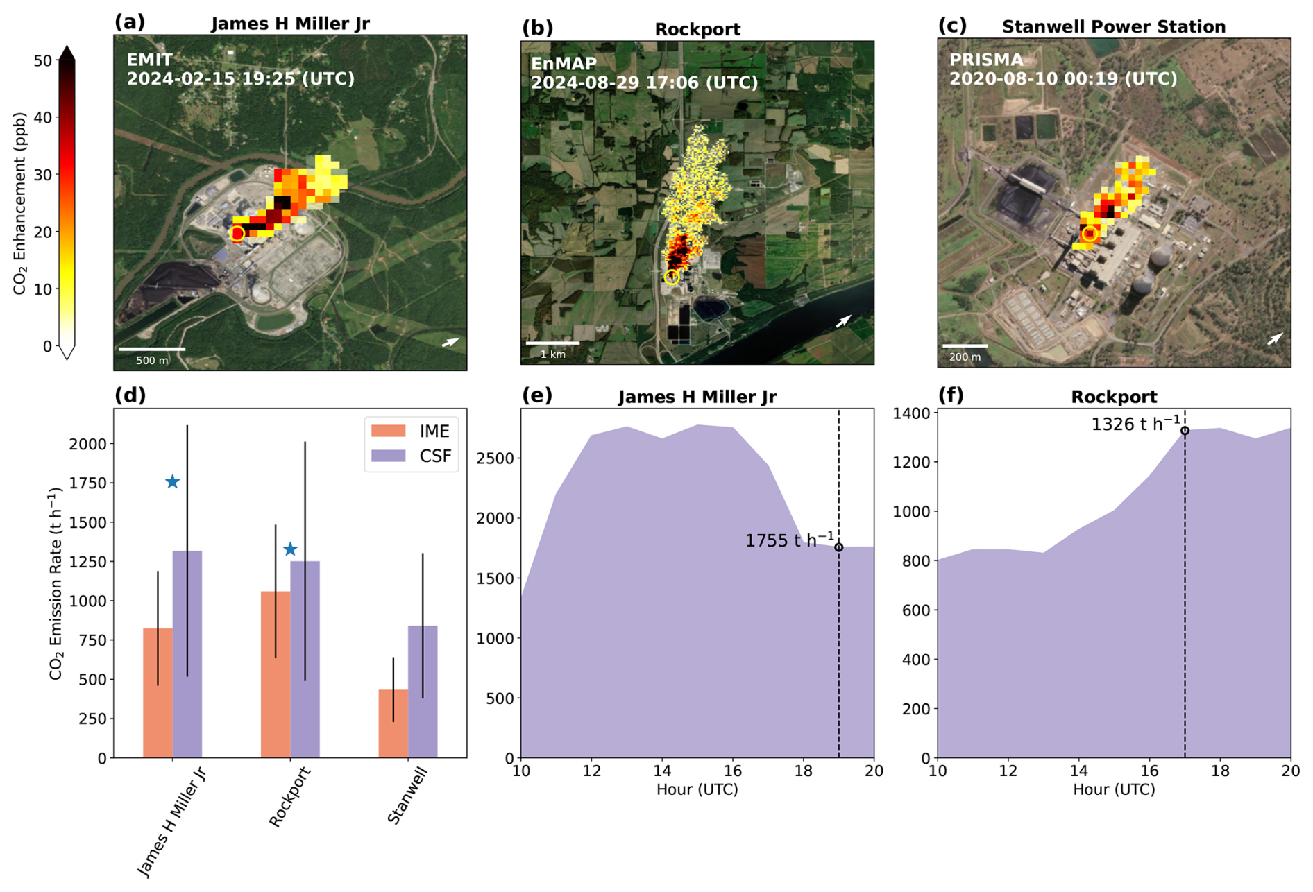
Figure 11 CO₂ plumes from power plants detected by (a) EMIT, (b) EnMAP, and (c) PRISMA. Instrument names and satellite overpass times are labeled in white text at the top of each panel. Yellow circles are identified plume source locations. Background ESRI imagery reproduced with permission as granted on Esri’s website for noncommercial scholarly use (Esri et al., 2022). Background imagery source: Esri|Powered by Esri. (d) Emission rate estimates derived using the IME and CSF methods. The blue stars are the CEMS-measured CO₂ emissions from the EPA database, interpolated at the time of the satellite overpass. (e, f) Time series of CEMS-measured CO₂ emissions from the EPA database. The dotted line indicates the satellite overpass time.

3.2 Carbon dioxide emissions

In addition to methane, HyperGas also supports quantifying CO₂ emission rates. Figure 11a–c show CO₂ plumes from three power plants: James H. Miller Jr. (AL, USA), Rockport (IN, USA), and Stanwell Power Station (Stanwell, Australia). The estimated emission rates range from 0.5 to 2 kt h⁻¹. On average, CSF estimates tend to be higher, particularly for the compact plume observed at the Stanwell Power Station and James H. Miller Jr. (Fig. 11d). For US power plants, we compare our estimates with stack-level estimates from Continuous Emission Monitoring Systems (CEMS, Fig. 11e and f; MEDUSA team D9.1, 2025). Although the CEMS reports generally fall within the uncertainty range of the CSF estimates, they tend to lie at the upper end of, or exceed, the IME results. This discrepancy may arise from plume simulations that assume surface-level sources and use only U₁₀ to represent wind speed, whereas the actual CO₂ emissions are released as hot, buoyant plumes at heights greater than 10 m. Consequently, using U₁₀ as a proxy may result in inaccurate wind speed calibrations for our observations, which could potentially affect emission estimates. As noted in the MEDUSA project (MEDUSA team D9.1, 2025), analyzed wind speeds at 100 m were on average 30 % higher than at 10 m. Future refinements could involve CO₂-specific simulations (Brunner et al., 2019) to improve this calibration by accounting for buoyant plumes released at altitude and relating the effective wind speed to a more representative reanalysis metric like the 100 m wind speed. Nevertheless, both IME and CSF estimates remain within their respective uncertainty bounds.

4 Conclusions

As hyperspectral satellite and airborne data become increasingly available, we have introduced the open-source package HyperGas, designed for retrieving atmospheric greenhouse gas enhancements, detecting, and quantifying greenhouse gas emissions. HyperGas provides modular tools and default settings to guide users through each stage of the analysis using an optimized and extendable workflow. We demonstrated how batch processing scripts and an interactive app enable both streamlined analysis and user-friendly interaction. For advanced users and developers, HyperGas offers the flexibility to implement custom algorithms at each step of the pipeline. This release enhances the standard matched filter retrieval by incorporating a lognormal matched filter and precise land/water masking. Users can further improve retrieval performance by applying their own pixel classification schemes and gas absorption coefficients, including aerosol scattering corrections (Feng et al., 2024).

We have also shown the integration of the open-source Python package tobac, originally developed for cloud tracking, to detect emission sources. Combined with a calibrated Chambolle total variation denoising (TV) filter, HyperGas generates plume masks that assist users in placing plume markers at source locations consistent with high-resolution visual imagery with the help of an interactive app.

For emission quantification, the package includes two established approaches, the integrated mass enhancement (IME) and the cross-sectional flux (CSF), along with default wind calibration settings. Users can assess uncertainties on the quantified emission rates, compare methods, and can modify the configuration for wind calibration routines. Further validation with additional methane controlled release experiments and hourly US. Environmental Protection Agency (EPA) CO₂ emission reports is recommended to determine the most appropriate method for various observational scenarios.

This initial release (HyperGas v1.0) provides robust functionality that can serve as the foundation for several additional features that can be developed in the future, including:

1. Automatic co-registration of PRISMA data (De Luca et al., 2024) to correct spatial misalignment between PRISMA imagery and actual Earth surface features.

2. Correction of smile effects (Guanter et al., 2021).

3. Support for a matched filter optimized with a sparse prior (Foote et al., 2020).

4. Integration of the Weighting Function Modified Differential Optical Absorption Spectroscopy (WFM-DOAS; Krings et al., 2011; Thorpe et al., 2014; Borchardt et al., 2021) method for gas retrievals.

5. Extension to additional trace gases, such as nitrogen dioxide (NO₂; Borger et al., 2025).

6. Addition of additional plume quantification approaches, such as the linear integrate mass enhancement method (Hakkarainen et al., 2025).

7. Support for upcoming global hyperspectral missions, including the Copernicus Hyperspectral Imaging Mission for the Environment (CHIME; Rast et al., 2021) and the Surface Biology and Geology mission (SBG; Cawse-Nicholson et al., 2021).

The main goal of HyperGas is to build a consistent and transparent system for quantifying anthropogenic emissions using hyperspectral observations. We welcome community contributions to expand its capabilities and to establish HyperGas as a foundation for ongoing methodological and scientific advancements.

Appendix A: Comparisons between matched filter and clustered matched filter

Figure A1 Retrieved methane enhancement using (a) the matched filter and (b) the cluster-tuned matched filter; (c) corresponding enhancement histograms; and (d) clusters applied in panel (b). The same scene is used in Fig. 10d.

Appendix B: HyperGas products

Table B1 HyperGas L2–L3 products table.