Evaluation of semi-implicit and explicit sedimentation approaches in the two-moment cloud microphysics scheme of ICON

In the ICOsahedral Nonhydrostatic (ICON) model, the Seifert-Beheng two-moment microphysics scheme is one approach to simulate clouds with different hydrometeor classes. In this bulk description, sedimentation is modeled by advecting the first two moments (number and mass densities) of the hydrometeor size distributions with velocities derived from fitting a generalized gamma distribution to the moments. This method implicitly relies on the diffusive properties of the numerical advection schemes to obtain results in closer agreement with the exact spectral solution. The implementation in ICON offers both a semi-implicit and largely untested explicit method for sedimentation. Currently, the semi-implicit scheme is substantially slower on graphics processing units (GPUs), which is particularly relevant considering the recent rise of GPUs in supercomputing; this raises the question of whether the explicit scheme is a viable alternative.

We provide a detailed examination of both sedimentation schemes, their differences, and underlying assumptions. Using idealized one-dimensional experiments, we identify a minor issue in the default semi-implicit scheme (flux limiter artifacts) and propose a solution. Additionally, we show that the explicit scheme exhibits less numerical diffusion, though some diffusion is crucial for accurate bulk sedimentation. Purely horizontal grid refinement leads to increased diffusion in the explicit scheme, whereas finer vertical resolutions may result in insufficient diffusion, especially for the explicit scheme. An analysis of six case studies with thunderstorms reveals that the explicit scheme gives rise to more jagged patterns in the hydrometeor profiles, although without concerning instabilities. Furthermore, some differences in hail and graupel precipitation rates can be attributed to different ways of considering the microphysical source terms (e.g., hydrometeor interactions) during the sedimentation step.

1 Introduction

Over the past two decades, a tremendous increase in computational power enabled many advances in numerical weather and climate models. Higher resolution in vertical and horizontal dimensions allows explicitly resolving deep convection, significantly improving precipitation forecasts (Lean et al., 2008; Kendon et al., 2014; Ban et al., 2015). Ensemble simulations enable probabilistic assessments (Bauer et al., 2015), and more sophisticated and thus expensive parameterizations such as multi-moment cloud microphysics can be used.

Particularly the rise of graphics processing units (GPUs) in supercomputing benefits weather and climate models due to higher memory bandwidths compared to traditional central processing units (CPUs), and the simulations' largely parallel nature (Owens et al., 2008; Leutwyler et al., 2016). However, enabling a sophisticated atmospheric model to execute well on both CPUs and GPUs from different generations and hardware manufacturers is very challenging, especially since a single source code with “high usability (...) by non-expert programmers” is strongly desirable due to typically “large developer, and even larger user communities” (Fuhrer et al., 2014). For GPU simulations with the Consortium for Small-Scale Modeling (COSMO) model, Fuhrer et al. (2018) have completely rewritten the dynamical core while porting the physical parameterizations with compiler directives. For the latter, they note, refactoring to recompute variables previously stored in memory played a crucial part, since floating point operations are much cheaper than data movement on modern architectures.

A similar approach with compiler directives was chosen for the ICOsahedral Nonhydrostatic (ICON) model (Zängl et al., 2015), where ETH Zurich, the Center for Climate Systems Modeling (C2SM), and the Swiss Federal Institute of Meteorology and Climatology (MeteoSwiss) had to invest significant resources to port ICON to GPUs for scientific research and operational weather forecasts (Project ICON-22, 2025) using the new Alps computing infrastructure (https://www.cscs.ch/computers/alps, last access: 7 May 2025) at the Swiss National Supercomputing Centre (CSCS). Still, significant challenges with code maintainability, adaptation to new architectures, and fragile workflows suggest that this approach is unsustainable in the long-term (Paredes et al., 2023).

During this combined effort, it was discovered that one specific physical parameterization, the two-moment cloud microphysics module (Seifert and Beheng, 2006) with some modifications (Segal and Khain, 2006; Blahak, 2008; Seifert, 2008; Noppel et al., 2010), performs particularly slowly on GPUs without significant refactoring. This microphysics scheme is commonly used in a variety of scientific studies, but also operationally by the German Meteorological Service (DWD) in the ICON-RUC (Rapid Update Cycle) model setup (Reinert et al., 2025) since 2024, and MeteoSwiss also considers employing it in the future. For sedimentation, which is part of the microphysics, ICON's default configuration utilizes a semi-implicit advection method based on a Crank-Nicolson discretization that also incorporates the remaining microphysical processes (source terms) with a predictor-corrector method. An alternative but largely untested explicit semi-Lagrangian method is also implemented, employing simple sequential operator splitting for sedimentation and the source terms. Such coupling may be less accurate, as hydrometeor interactions with thin cloud layers could be entirely missed for large sedimentation velocities. However, this explicit variant performs much better on GPUs, shown by runtime measurements in Table 1, which will be discussed in detail in Sect. 2.2.

Table 1 Runtimes using the two-moment sedimentation scheme as implemented in ICON version 2024.10. We report the two-moment microphysics (total average across processes) and total simulation (in brackets) runtime in seconds, as measured by ICON's built-in timing routines. The runtime for three identical simulations and their mean is shown, using the setup from Sect. 4, except for disabled output. We use a single Grace-Hopper node, consisting of four NVIDIA GH200 superchips, of the Alps supercomputer.

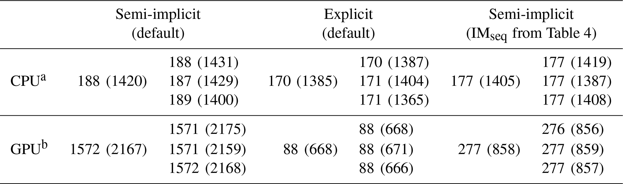
^a Total $\mathrm{4}\times \mathrm{72}=\mathrm{288}$ processes, 286 for CPU computation, 1 for I/O, 1 for prefetching
^b Total 5 processes, 4 for GPU computation, 1 for prefetching

In the future, the resolution of weather and climate models can be expected to further increase, as it improves the representation of clouds and convection (Miyamoto et al., 2013; Heinze et al., 2017; Stevens et al., 2020; Omanovic et al., 2024), and terrain-induced circulations (Schmidli et al., 2018; Heim et al., 2020; Mikkola et al., 2023), in addition to reducing the numerical discretization and coupling errors. Conversely, the two-moment bulk sedimentation description benefits from some numerical diffusion errors to suppress unphysical shockwaves introduced by the parameterization (Wacker and Seifert, 2001), and thus diffusive errors may also be relied upon for stability of the sedimentation schemes.

In light of those aspects, this paper aims to investigate whether or to what extent the explicit sedimentation scheme is a viable alternative to the semi-implicit variant. Currently, the semi-implicit sedimentation scheme is only documented for its initial implementation in the COSMO one-moment scheme (Doms et al., 2021, Sect. 5.2.4), which does not cover several modifications made for use in ICON's two-moment microphysics. The explicit scheme considered here is documented and referred to as the “boxtracking” scheme by Blahak (2020), which was meant as a first improvement over a scheme with a significantly flawed fall speed approximation in the flux calculation. Thus, we first provide a concise overview of both sedimentation methods in Sect. 2, without neglecting small but ultimately important implementation details. Using insights from those numerical descriptions, single-column experiments with pure sedimentation (Sect. 3), and case studies based on full ICON simulations (Sect. 4), we investigate and evaluate the impact of switching between the semi-implicit and explicit schemes, and further configuration options. In the conclusions (Sect. 5), we summarize our findings and give recommendations for future model setups.

2 Sedimentation schemes in ICON

2.1 Sedimentation description

We start by providing a brief overview of ICON's two-moment microphysics sedimentation description, closely following Wacker and Seifert (2001) and Seifert and Beheng (2006). In general, the hydrometeors are categorized into different classes, namely cloud droplets, rain, cloud ice, snow, graupel, and hail. Each hydrometeor class is modeled by a distinct size distribution with two free parameters, determined by the local number and mass density, i.e., the first two moments of this distribution. Thus, the two-moment description's aim is to describe all microphysical processes, including sedimentation, in terms of those two moments.

The starting point for sedimentation is the one-dimensional spectral budget equation for the number density size distribution f, modeling the pure sedimentation process in vertical direction for different hydrometeors:

$$\begin{array}{}\text{(1)}& {\displaystyle \frac{\partial }{\partial t}}f(z,t,x)=-{\displaystyle \frac{\partial }{\partial z}}\left[v\right(\mathit{\rho },x)\cdot f(z,t,x\left)\right].\end{array}$$

Specifically, ${\int }_{x_{\mathrm{1}}}^{x_{\mathrm{2}}}f(z,t,x)\mathrm{d}x$ describes the number density of particles with mass x between x₁ and x₂, and $v(\mathit{\rho },x)\le \mathrm{0}$ is the sedimentation velocity depending on particle mass x and atmospheric density ρ. Sources and sinks, e.g., hydrometeor interactions, will be introduced later in Eq. (9). Other processes such as wind-driven advection, turbulent diffusion and saturation adjustment are treated outside ICON's microphysics module in a time-split manner (Reinert et al., 2024). The moment budget equations arise from integrating Eq. (1) over the mass x. After defining the mth moment M_m and its sedimentation velocity ${\stackrel{\mathrm{‾}}{v}}_m$,

$$\begin{array}{}\text{(2)}& {\displaystyle }{M}_m& {\displaystyle }=\underset{\mathrm{0}}{\overset{\mathrm{\infty }}{\int }}f(z,t,x)\cdot x^m\mathrm{d}x\text{(3)}& {\displaystyle }{\stackrel{\mathrm{‾}}{v}}_m& {\displaystyle }={\displaystyle \frac{{\int }_{\mathrm{0}}^{\mathrm{\infty }}v(\mathit{\rho },x)\cdot f(z,t,x)\cdot x^m\mathrm{d}x}{M_m}},\end{array}$$

an advection equation for each moment M_m is obtained:

$$\begin{array}{}\text{(4)}& {\displaystyle \frac{\partial }{\partial t}}{M}_m=-{\displaystyle \frac{\partial }{\partial z}}[{\stackrel{\mathrm{‾}}{v}}_m\cdot M_m].\end{array}$$

However, evaluating ${\stackrel{\mathrm{‾}}{v}}_m$ still requires knowledge about the entire size distribution $f(z,t,x)$, rather than just the moments M₀ and M₁. To address this, f is approximated by fitting a generalized Γ-distribution to the moments:

$$\begin{array}{}\text{(5)}& f\left(x\right)\approx g\left(x\right):=A{x}^{\mathit{\nu }}\exp (-\mathit{\lambda }{x}^{\mathit{\mu }}).\end{array}$$

In the case of ice phase hydrometeors (ice crystals, snow, graupel, hail), ν and μ are fixed dimensionless shape parameters, whereas A and λ are to be determined by the two moments. For rain, μ can optionally be further parameterized by a relation to the raindrop diameter (Seifert, 2008). After defining a parameterized relation between the particle mass x and sedimentation speed, e.g., a power law for ice phase hydrometeors, combined with a scaling factor $({\mathit{\rho }}_{\mathrm{0}}/\mathit{\rho }{)}^{\mathit{\gamma }}$ to account for the dependence of the terminal fall speed on air density ρ, it is possible to evaluate the speed of the mth moment of the Γ-distribution g(x). Writing N:=M₀ and L:=M₁ for the number and mass densities, respectively, we obtain:

$$\begin{array}{}\text{(6)}& {\displaystyle }{v}_{\text{frozen}}\left(x\right)=-\mathit{\alpha }{x}^{\mathit{\beta }}{\left({\displaystyle \frac{{\mathit{\rho }}_{\mathrm{0}}}{\mathit{\rho }}}\right)}^{\mathit{\gamma }},\text{(7)}& {\displaystyle }\begin{array}{rl}{v}_m(N,L)& ={\displaystyle \frac{{\int }_{\mathrm{0}}^{\mathrm{\infty }}{v}_{\text{frozen}}\left(x\right)x^{m}g\left(x\right)\mathrm{d}x}{M_m}}\\ & =-c_m\cdot {\left({\displaystyle \frac{L}{N}}\right)}^{\mathit{\beta }}\cdot {\left({\displaystyle \frac{{\mathit{\rho }}_{\mathrm{0}}}{\mathit{\rho }}}\right)}^{\mathit{\gamma }}\end{array}\text{(8)}& {\displaystyle }{c}_m:=\mathit{\alpha }{\displaystyle \frac{\mathrm{\Gamma }\left(\frac{m+\mathit{\nu }+\mathit{\beta }+\mathrm{1}}{\mathit{\mu }}\right)}{\mathrm{\Gamma }\left(\frac{m+\mathit{\nu }+\mathrm{1}}{\mathit{\mu }}\right)}}{\left[{\displaystyle \frac{\mathrm{\Gamma }\left(\frac{\mathit{\nu }+\mathrm{1}}{\mathit{\mu }}\right)}{\mathrm{\Gamma }\left(\frac{\mathit{\nu }+\mathrm{2}}{\mathit{\mu }}\right)}}\right]}^{\mathit{\beta }}.\end{array}$$

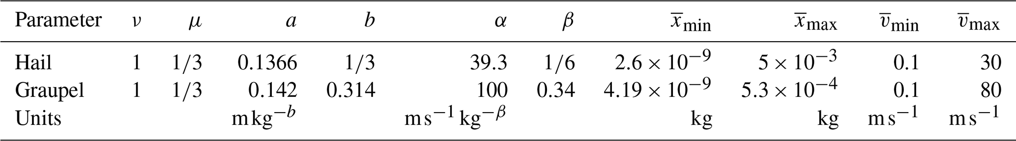
For rain, the same procedure is applied to compute the approximate velocities of the moments, but instead of a power law as in Eq. (6), an Atlas-type fall speed relation is used (Seifert et al., 2014). For simplicity, we just focus on the graupel and hail parameterizations, and provide the specific values used by ICON in Table 2.

Table 2 Default hail and graupel parameter choices, as defined in the ICON version 2024.10 source code (ICON partnership (MPI-M, DWD, DKRZ, KIT, and C2SM), 2024). The parameters a, b describe the relation to the particle diameter D(x)=ax^b. Further, for scaling the sedimentation speed depending on the atmospheric density ρ(z) using Eq. (6), the parameters γ=0.4 and ρ₀=1.225 kg m⁻³ are fixed and independent of the hydrometeor class.

Finally, when also including the source terms that encompass the remaining microphysical processes, the equation to solve for each hydrometeor class is:

$$\begin{array}{}\text{(9)}& {\displaystyle \frac{\partial }{\partial t}}\left[\begin{array}{c}N\\ L\end{array}\right]=-{\displaystyle \frac{\partial }{\partial z}}\left(\left[\begin{array}{c}{v}_{\mathrm{0}}(N,L)\cdot N\\ v_{\mathrm{1}}(N,L)\cdot L\end{array}\right]\right)+\left[\begin{array}{c}{Q}_N(N,L,\mathrm{\dots })\\ Q_L(N,L,\mathrm{\dots })\end{array}\right].\end{array}$$

Since the source terms Q_N, Q_L model all hydrometeor interactions including their formation and dissipation, they not only depend on the moments of the current hydrometeor class, but on the entire local atmospheric model state.

It is important to acknowledge the difference to the spectral formulation in Eq. (1). Whereas the spectral description can be understood as infinitely many linear advection equations, the two-moment bulk description consists of two quasilinear advection equations, coupled through non-linear velocities (and source terms). This is a fundamentally different structure, particularly, only the bulk description leads to the emergence of unrealistic shock waves (Wacker and Seifert, 2001). In practice, this can mostly be compensated by the deliberate use of diffusive numerical schemes for solving Eq. (9).

Of course, then the question of what the optimal amount of diffusion is arises. When only relying on numerical diffusion, the specific amount typically depends on the advection speed and discretization (Δz and/or Δt), and thus can vary significantly across the domain. Generally, too little diffusion will result in spurious shock waves, whereas too much diffusion produces overly smooth fields that may be unable to capture fine structures of clouds, and reduces size sorting. It should be noted that the latter may actually be desired, since size sorting is often too pronounced in two-moment schemes (Milbrandt and Yau, 2005; Mansell, 2010). To find the right balance between those effects, in theory, we would suggest deriving the optimal diffusion coefficient directly from the spectral formulation, e.g., by computing a Taylor expansion in space of the spectral solution's moments, giving rise to an ideal local diffusion coefficient that depends on the moment m and hydrometeor concentrations N, L themselves. In principle, such a coefficient could be combined with knowledge about the diffusive error terms of the numerical schemes used in sedimentation and tracer advection, allowing a tight control over diffusion across resolutions. However, the benefits of such a complex approach appear questionable, especially compared to all other approximations and uncertainties that exist in the parameterizations of cloud microphysical processes.

2.2 Semi-implicit scheme

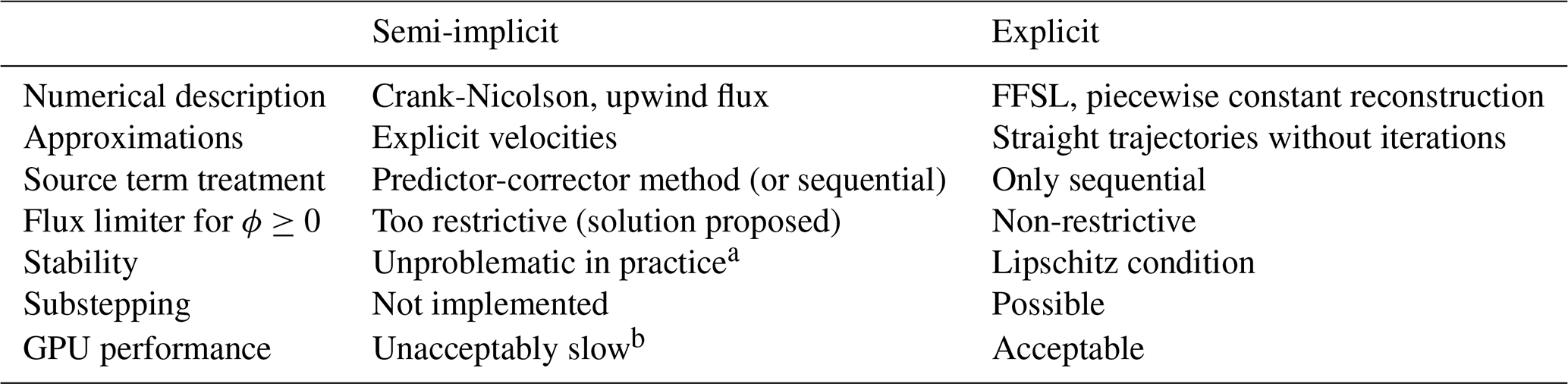
For clarity and conciseness, we will use ϕ to describe both N and L for all hydrometeor classes. Likewise, we will use the generic source term Q and velocity v; these refer to the source term and velocity function, respectively, for the respective moment and hydrometeor class. Furthermore, Table 3 provides a brief summary over both sedimentation schemes, which will be presented in great detail next.

Table 3 Brief overview over the two sedimentation schemes as implemented in ICON version 2025.04.

^a The explicit velocity approximation from Eq. (12) theoretically impacts stability.
^b In case of predictor-corrector source term treatment, otherwise only slightly slower than the explicit scheme. Table 1 lists runtimes of respective configurations.

The semi-implicit scheme is the default method to solve Eq. (9) in ICON. Originally used in the COSMO one-moment scheme (Doms et al., 2021), it was adapted and modified for the two-moment microphysics of ICON. It employs a mass-conserving Crank-Nicolson discretization with upwind flux for the advection terms, and an explicit approximation for velocities to avoid solving non-linear systems. In the default configuration, source terms are handled by a predictor-corrector method, which intertwines the sources with sedimentation. The default semi-implicit scheme's update step is given by

$$\begin{array}{}\text{(10)}& {\displaystyle }\begin{array}{rl}{\mathit{\varphi }}_k^{*}& ={\left(\mathrm{1}-{\displaystyle \frac{\mathrm{\Delta }t}{\mathrm{2}\mathrm{\Delta }{z}_k}}{\stackrel{\mathrm{̃}}{v}}_k^{(n+\mathrm{1})}\right)}^{-\mathrm{1}}\\ & \cdot \left[{\mathit{\varphi }}_k^{\left(n\right)}-{\displaystyle \frac{\mathrm{\Delta }t}{\mathrm{2}\mathrm{\Delta }{z}_k}}\left(\right(\stackrel{\mathrm{̃}}{v}\mathit{\varphi }{)}_{k-\mathrm{1}}^{(n+\mathrm{1})}+(v\mathit{\varphi }{)}_{k-\mathrm{1}}^{\left(n\right),\text{lim}}-(v\mathit{\varphi }{)}_k^{\left(n\right),\text{lim}})\right]\end{array}\text{(11)}& {\displaystyle }\begin{array}{rl}{\mathit{\varphi }}_k^{(n+\mathrm{1})}& ={\left(\mathrm{1}-{\displaystyle \frac{\mathrm{\Delta }t}{\mathrm{2}\mathrm{\Delta }{z}_k}}{\stackrel{\mathrm{̃}}{v}}_k^{(n+\mathrm{1})}\right)}^{-\mathrm{1}}\\ & \cdot [{\mathit{\varphi }}_k^{\left(n\right)}-{\displaystyle \frac{\mathrm{\Delta }t}{\mathrm{2}\mathrm{\Delta }{z}_k}}((\stackrel{\mathrm{̃}}{v}\mathit{\varphi }{)}_{k-\mathrm{1}}^{(n+\mathrm{1})}+(v\mathit{\varphi }{)}_{k-\mathrm{1}}^{\left(n\right),\text{lim}}-\left(v\mathit{\varphi }{)}_k^{\left(n\right),\text{lim}}\right)\\ & +Q_k\left({\mathit{\varphi }}_k^{*}\right)\mathrm{\Delta }t],\end{array}\end{array}$$

where the sub- and superscripts are level and time indices, respectively. Notably, ICON uses a reversed level indexing convention compared to the z axis direction, i.e., level k=1 is the uppermost level. Furthermore, ρ is assumed constant in time during a single update step, and writing $v_k^{\left(n\right)}$ for $v_m(N_k^{\left(n\right)},L_k^{\left(n\right)})$, the implicit velocity $v_k^{(n+\mathrm{1})}$ was replaced by the explicit approximation

$$\begin{array}{}\text{(12)}& {\stackrel{\mathrm{̃}}{v}}_k^{(n+\mathrm{1})}:={\displaystyle \frac{\mathrm{1}}{\mathrm{2}}}(v_k^{\left(n\right)}+v_{k-\mathrm{1}}^{\left(n\right)}).\end{array}$$

This approximation, in combination with the upwind flux, greatly reduces the computational effort since it eliminates the need to solve any (non-linear) systems of equations with iterative methods. Instead, Eq. (11) can simply be applied level by level, i.e., starting from the domain's top at k=1, simultaneously for all hydrometeor classes and moments. We should add that the velocity approximation in Eq. (12) is clearly different from the original COSMO implementation, where ${\stackrel{\mathrm{̃}}{v}}_k^{(n+\mathrm{1})}=v\left(\frac{\mathrm{1}}{\mathrm{2}}\right({\mathit{\varphi }}_k^{\left(n\right)}+{\mathit{\varphi }}_{k-\mathrm{1}}^{(n+\mathrm{1})}\left)\right)$ was used (Doms et al., 2021, p. 52); especially note how the ICON implementation only takes values from time step n. In Sect. 2.4, we will mention how an interaction of this approximation with Eq. (26) could cause an artificial shock wave, although this is almost irrelevant in practice.

For physical reasons, mass and number concentrations should also remain nonnegative during the update step. This is achieved, without violating mass conservation, by applying a flux limiter:

$$\begin{array}{}\text{(13)}& (v\mathit{\varphi }{)}_k^{\left(n\right),\text{lim1}}:=max\mathit{\{}(v\mathit{\varphi }{)}_k^{\left(n\right)},(\stackrel{\mathrm{̃}}{v}\mathit{\varphi }{)}_{k-\mathrm{1}}^{(n+\mathrm{1})}+\left(v\mathit{\varphi }{)}_{k-\mathrm{1}}^{\left(n\right),\text{lim1}}\mathit{\right\}}.\end{array}$$

This limiter enforces that the square bracket in Eq. (10) remains $\ge {\mathit{\varphi }}_k^{\left(n\right)}$, and thus ${\mathit{\varphi }}_k^{*}\ge \mathrm{0}$ as well. However, this limiter is ultimately arbitrary and too restrictive, since it does not consider the effect of time integration. Hence, we propose an improved flux limiter, which only activates when ϕ<0 would emerge during time integration. In other words, we should only enforce that the square bracket in Eq. (10) remains ≥0, as opposed to $\ge {\mathit{\varphi }}_k^{\left(n\right)}$:

$$\begin{array}{}\text{(14)}& \begin{array}{rl}& (v\mathit{\varphi }{)}_k^{\left(n\right),\text{lim2}}:=\\ & max\left\{(v\mathit{\varphi }{)}_k^{\left(n\right)},(\stackrel{\mathrm{̃}}{v}\mathit{\varphi }{)}_{k-\mathrm{1}}^{(n+\mathrm{1})}+(v\mathit{\varphi }{)}_{k-\mathrm{1}}^{\left(n\right),\text{lim2}}-{\displaystyle \frac{\mathrm{2}\mathrm{\Delta }{z}_k}{\mathrm{\Delta }t}}{\mathit{\varphi }}_k^{\left(n\right)}\right\}.\end{array}\end{array}$$

Notably, both flux limiter versions are also sufficient to guarantee ${\mathit{\varphi }}_k^{(n+\mathrm{1})}\ge \mathrm{0}$ when used in Eq. (11) where the sources are applied, since ICON's source term computation also guarantees ${\mathit{\varphi }}_k^{*}+Q_k\left({\mathit{\varphi }}_k^{*}\right)\mathrm{\Delta }t\ge \mathrm{0}$. Note that we use the generic ^lim superscript to refer to either of the two flux limiters from Eqs. (13) and (14).

Instead of the predictor-corrector method described by Eqs. (10) and (11), it is also possible to treat the source terms with sequential operator splitting, i.e., by simply integrating the source terms before applying the sedimentation step:

$$\begin{array}{ll}\text{(15)}& {\displaystyle }& {\displaystyle }{\mathit{\varphi }}^{\left(n\right)}\leftarrow {\mathit{\varphi }}^{\left(n\right)}+Q\left({\mathit{\varphi }}^{\left(n\right)}\right)\mathrm{\Delta }t{\displaystyle }& {\displaystyle }{\mathit{\varphi }}_k^{(n+\mathrm{1})}={\left(\mathrm{1}-{\displaystyle \frac{\mathrm{\Delta }t}{\mathrm{2}\mathrm{\Delta }{z}_k}}{\stackrel{\mathrm{̃}}{v}}_k^{(n+\mathrm{1})}\right)}^{-\mathrm{1}}\\ \text{(16)}& {\displaystyle }& {\displaystyle }\cdot \left[{\mathit{\varphi }}_k^{\left(n\right)}-{\displaystyle \frac{\mathrm{\Delta }t}{\mathrm{2}\mathrm{\Delta }{z}_k}}\left(\right(\stackrel{\mathrm{̃}}{v}\mathit{\varphi }{)}_{k-\mathrm{1}}^{(n+\mathrm{1})}+(v\mathit{\varphi }{)}_{k-\mathrm{1}}^{\left(n\right),\text{lim}}-(v\mathit{\varphi }{)}_k^{\left(n\right),\text{lim}})\right].\end{array}$$

In this variant, the source terms are computed in the entire domain at once, as opposed to the level-wise calculation required in the predictor-corrector configuration. In fact, this would improve the semi-implicit scheme's GPU performance significantly, but makes virtually no difference for CPUs: Currently, the source term computation has very high overhead on GPUs due to a large number of GPU kernel launches. Since this overhead remains fixed regardless of the computational domain's size, the combined overhead of the level-wise calculation exceeds that of the all-at-once approach by a factor equal to the number of levels. On GPUs, this accounts for over 85 % of the runtime difference between the default semi-implicit and explicit sedimentation schemes as shown in Table 1, since the explicit scheme only offers the sequential source term treatment (see Sect. 2.3). Still, we see no fundamental reason why all variants of the semi-implicit scheme could not reach GPU runtimes similar to the explicit scheme. This would, however, require a rather substantial rewrite of the implementation.

2.3 Explicit scheme

The explicit scheme for hydrometeor sedimentation is a rather simple, conservative first-order flux-form semi-Lagrangian (FFSL) method using straight-line trajectories and a piecewise constant reconstruction (Blahak, 2020). Furthermore, sedimentation and source terms are treated with operator splitting, i.e., simply applied sequentially, analogous to Eqs. (15) and (16) for the semi-implicit scheme. The explicit method's update step is described by

$$\begin{array}{}\text{(17)}& {\displaystyle }{\mathit{\varphi }}^{\left(n\right)}\leftarrow {\mathit{\varphi }}^{\left(n\right)}+Q\left({\mathit{\varphi }}^{\left(n\right)}\right)\mathrm{\Delta }t\text{(18)}& {\displaystyle }{\mathit{\varphi }}_k^{(n+\mathrm{1})}={\mathit{\varphi }}_k^{\left(n\right)}-{\displaystyle \frac{\mathrm{\Delta }t}{\mathrm{\Delta }{z}_k}}({\stackrel{\mathrm{‾}}{P}}_{k-\frac{\mathrm{1}}{\mathrm{2}}}^{\text{lim}}-{\stackrel{\mathrm{‾}}{P}}_{k+\frac{\mathrm{1}}{\mathrm{2}}}^{\text{lim}}),\end{array}$$

where the time-averaged fluxes $\stackrel{\mathrm{‾}}{P}$ are approximated by

$$\begin{array}{}\text{(19)}& {\displaystyle }{\stackrel{\mathrm{‾}}{P}}_{k+\frac{\mathrm{1}}{\mathrm{2}}}\approx -{\displaystyle \frac{\mathrm{1}}{\mathrm{\Delta }t}}\sum _{l=\mathrm{0}}^{k-\mathrm{1}}{\mathit{\varphi }}_{k-l}\cdot (z_{\text{up}}-z_{\text{low}})\text{(20)}& {\displaystyle }\begin{array}{rl}& z_{\text{up}}=min[z_{k+\frac{\mathrm{1}}{\mathrm{2}}-l-\mathrm{1}},z_{k+\frac{\mathrm{1}}{\mathrm{2}}}+|v_{k-l}\left|\mathrm{\Delta }t\right],\\ & z_{\text{low}}=min[z_{k+\frac{\mathrm{1}}{\mathrm{2}}-l},z_{\text{up}}]\end{array}\end{array}$$

with the flux limiter

$$\begin{array}{}\text{(21)}& {\stackrel{\mathrm{‾}}{P}}_{k+\frac{\mathrm{1}}{\mathrm{2}}}^{\text{lim}}:=max\left[{\stackrel{\mathrm{‾}}{P}}_{k+\frac{\mathrm{1}}{\mathrm{2}}},{\stackrel{\mathrm{‾}}{P}}_{k-\frac{\mathrm{1}}{\mathrm{2}}}^{\text{lim}}-{\mathit{\varphi }}_k^{\left(n\right)}{\displaystyle \frac{\mathrm{\Delta }{z}_k}{\mathrm{\Delta }t}}\right].\end{array}$$

This flux limiter simply ensures ${\mathit{\varphi }}_k^{(n+\mathrm{1})}\ge \mathrm{0}$, which can easily be seen from inserting Eq. (21) into Eq. (18), while also conserving mass. A geometric interpretation for the flux computation in Eq. (19) is helpful, illustrated by Fig. 1. For each cell k−l, a linear trajectory with slope $\mathrm{1}/v_{k-l}^{\left(n\right)}$ is assumed, i.e., the cell is notionally moved by the distance $v_{k-l}^{\left(n\right)}\mathrm{\Delta }t$ to obtain its arrival region. Then, z_up−z_low simply describes how much of the notionally moved cell has passed by the cell face at location z_k+½, as visualized in Fig. 1. Thus, ${\mathit{\varphi }}_{k-l}\cdot (z_{\text{up}}-z_{\text{low}})$ describes the integrated amount of ϕ_k−l that has passed the cell face z_k+½ under the assumption of a cell-wise constant ϕ.

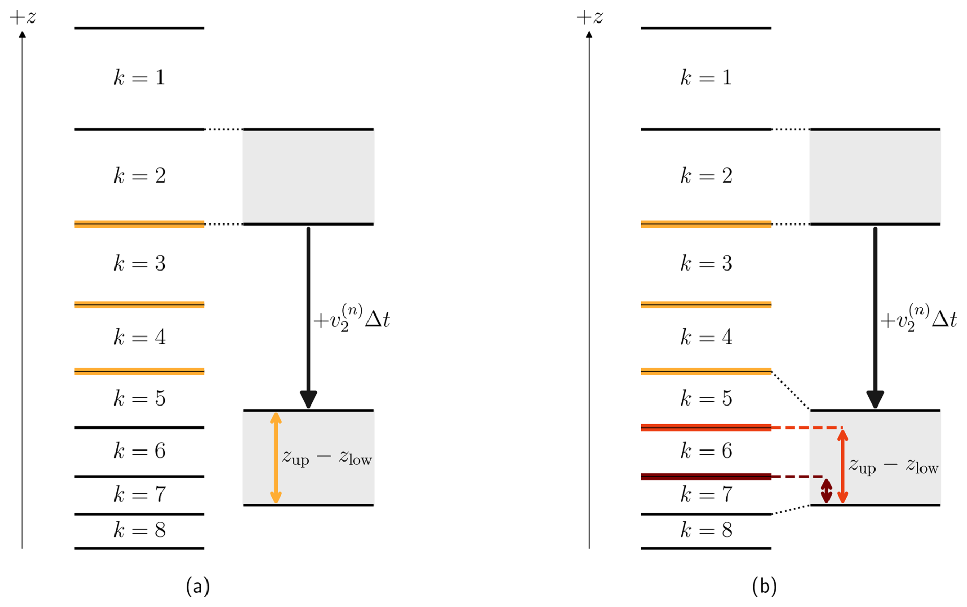
Figure 1 Visualization of the flux computation for the explicit method as described by Eq. (19). The index k, decreasing with height z, denotes levels separated by cell faces (horizontal lines). The contribution of level $k-l=\mathrm{2}$ to all fluxes ${\stackrel{\mathrm{‾}}{P}}_{k+\frac{\mathrm{1}}{\mathrm{2}}}$ is shown, i.e., when $k-l=\mathrm{2}$ is encountered in the sum in Eq. (19). The cell $k-l=\mathrm{2}$ (shaded gray) is notionally moved along its linear trajectory with slope $\mathrm{1}/v_{k-l}^{\left(n\right)}$, i.e., displaced by the distance $v_{k-l}^{\left(n\right)}\mathrm{\Delta }t$ as illustrated by the black arrow. (a) Cell faces at locations z_k+½ for $k\in \mathit{\{}\mathrm{2},\mathrm{3},\mathrm{4}\mathit{\}}$, highlighted in yellow, are fully traversed by the notionally moved cell. For those cell faces, the flux contribution from level $k-l=\mathrm{2}$ is ${\mathit{\varphi }}_{\mathrm{2}}^{\left(n\right)}\mathrm{\Delta }{z}_{\mathrm{2}}/\mathrm{\Delta }t$, i.e., $z_{\text{up}}-z_{\text{low}}=\mathrm{\Delta }{z}_{\mathrm{2}}$ per Eq. (20), as shown by the yellow arrow. As the time integration with Eq. (18) only depends on the flux difference ${\stackrel{\mathrm{‾}}{P}}_{k-\frac{\mathrm{1}}{\mathrm{2}}}-{\stackrel{\mathrm{‾}}{P}}_{k+\frac{\mathrm{1}}{\mathrm{2}}}$, the values in levels $k\in \mathit{\{}\mathrm{3},\mathrm{4}\mathit{\}}$ remain unaffected by level $k-l=\mathrm{2}$. (b) Cell faces partially traversed by the notionally moved cell $k-l=\mathrm{2}$, marked by the red and dark red lines, are also considered. Here, the weighting z_up−z_low corresponds to the distance from the moved cell's lower face, shown by the red arrows. Consequently, values from level $k-l=\mathrm{2}$ are distributed to levels $k\in \mathit{\{}\mathrm{5},\mathrm{6},\mathrm{7}\mathit{\}}$. The extent of numerical diffusion thus depends on how closely the moved cell aligns with the actual cell faces.

In contrast to typical explicit Eulerian methods, this FFSL scheme is not constrained by the Courant number $C:=\left|v\right|\mathrm{\Delta }t/\mathrm{\Delta }z$, however, a different restriction appears. Smolarkiewicz and Pudykiewicz (1992) derive a limitation on the Lipschitz number ℬ as a trajectory iteration convergence condition:

$$\begin{array}{}\text{(22)}& \mathcal{B}:=\left|{\displaystyle \frac{\partial v}{\partial z}}\right|\mathrm{\Delta }t<\mathrm{1}.\end{array}$$

This can be interpreted as preventing the trajectories from intersecting, thus controlling “topological issues (connectivity preservation) in computational flows” (Smolarkiewicz and Pudykiewicz, 1992). Although our simple FFSL scheme does not iterate on the trajectories to obtain a higher-order approximation, e.g., as outlined by Staniforth and Côté (1991), this Lipschitz condition remains highly relevant: ℬ>1 still leads to issues with the flow's connectivity and may thus introduce spurious oscillations, e.g., when fluid particles originally located in adjacent cells end up several cells apart after a single time step, leaving an empty gap in-between.

Usually, the Lipschitz condition is far more lenient than the CFL condition (C≤1) of typical explicit Eulerian methods (e.g., Skamarock, 2006). In our case however, where the velocity non-linearly depends on N and L, one can imagine a case where v=0 in one cell, and $\left|v\right|\gg \mathrm{0}$ adjacently. In other words, the Lipschitz condition may reduce to $\mathcal{B}=\left|v\right|\mathrm{\Delta }t/\mathrm{\Delta }z<\mathrm{1}$ in the worst case, which is similar to the CFL condition. Still, a Lipschitz condition violation does not necessarily lead to severe stability issues, e.g., Smolarkiewicz and Pudykiewicz (1992) only conclude that the numerical solution becomes “meaningless” for ℬ>1. For the explicit sedimentation scheme discussed here, we observe that minor vertical oscillations of the mean hydrometeor mass $L/N$ are sometimes introduced in case of C>1, even for ℬ≪1, presumably as a combined effect of how the trajectories align with cell faces (see Fig. 1), and the two moments' different sedimentation speed. Since this then leads to velocity variations, such perturbations can further grow and propagate if diffusive processes are unable to provide enough smoothing, until reaching ℬ>1 as illustrated by Fig. B1. When the Lipschitz condition is violated, we often see the emergence of rapid oscillations, however, such violations may also remain brief and not cause significant effects. If oscillations appear, they do not blow up, thanks to mass conservation and applied mean particle mass bounds, and eventually exit the domain upon reaching the ground. Furthermore, in non-idealized scenarios, smoothing effects caused by tracer advection and the source terms alleviate the problem by reducing the spatial variations of N and L, thus also of v and the Lipschitz number ℬ. Since turbulent diffusion is not applied to graupel, hail, and rain (only cloud droplets in our configuration), it does not contribute to those smoothing effects where relevant for sedimentation.

Finally, the explicit scheme also supports so-called sedimentation substepping for the rapidly sedimenting hydrometeor classes (rain, graupel, hail), where the explicit sedimentation update step described by Eq. (18) is simply applied repeatedly, i.e., N_sub times with a reduced time step $\mathrm{\Delta }t/N_{\text{sub}}$. This is controlled by an internal code switch, which is disabled by default because of reproducability problems in the current ICON version when the domain decomposition changes, i.e., when the number of processes is modified. Importantly, substepping only applies to sedimentation, such that the source term application given in Eq. (17) remains unaffected. Presently, the number of substeps is chosen to keep C≲1 based on an upper bound for hydrometeor velocities ${\stackrel{\mathrm{‾}}{v}}_{\text{max}}$, as used later in Eq. (26):

$$\begin{array}{}\text{(23)}& N_{\text{sub}}=\lceil {\stackrel{\mathrm{‾}}{v}}_{\text{max}}\mathrm{\Delta }t/\underset{k}{min}\left(\mathrm{\Delta }{z}_k\right)\rceil .\end{array}$$

We should note that ${\stackrel{\mathrm{‾}}{v}}_{\text{max}}$ is enforced prior to scaling with atmospheric density in Eq. (26), such that C≤1 is not always strictly guaranteed. Further, the aforementioned reproducability problem is caused by the computation of min_k(Δz_k), which is done over the local domain (determined by partitioning the entire simulation region according to the number of processes). Therefore, min_k(Δz_k) might vary slightly across the processes, depending on the domain decomposition. This issue is reported to the ICON developers; and to improve the reproducability of our simulations, we manually fix N_sub to the highest value encountered across the entire simulation domain.

Clearly, substepping lowers both the Courant and Lipschitz numbers, and should therefore reduce the occurrence rate of Lipschitz condition violations which in turn decreases spurious oscillations at the cost of higher computational cost and more numerical diffusion.

2.4 Number and velocity restrictions

In practice, the bulk sedimentation Eq. (9), with velocities obtained from Eq. (7) comprises some challenges, particularly when N and L are close to or exactly zero. In such cases, the mean mass $\stackrel{\mathrm{‾}}{x}=L/N$, and consequently the bulk velocities v_m(N,L), are either extremely sensitive to small changes, or not well-defined at all. Furthermore, $\stackrel{\mathrm{‾}}{x}$, and thus v_m(N,L) too, are unbounded, and we must address physical consistency issues like obtaining nonzero mass (L>0) without particles (N=0). Notably, such problematic conditions are mostly observed on the leading edge of a precipitation column, since L sediments faster than N. This is also precisely where excessive size sorting (and consequently spurious reflectivity growth) can be observed, compared to the spectral formulation. Various techniques have been tried to control this issue, e.g., by applying corrections based on the diagnosed reflectivity and/or adjusting distribution shape parameters (Milbrandt and Yau, 2005; Mansell, 2010).

Therefore, the choices made for handling edge cases with small N, L ultimately impact the numerical results quite significantly, and thus we will need provide further implementation details for ICON. First, just before each microphysics step, number concentrations are adjusted to respect lower and upper bounds for the mean particle mass:

$$\begin{array}{}\text{(24)}& {\displaystyle }& {\displaystyle }\text{clamp}(y,y_{\text{min}},y_{\text{max}}):=min(max(y,y_{\text{min}}),y_{\text{max}})\text{(25)}& {\displaystyle }& {\displaystyle }N\leftarrow \left\{\begin{array}{ll}\text{clamp}\left(N,\frac{L}{{\stackrel{\mathrm{‾}}{x}}_{\text{max}}},\frac{L}{{\stackrel{\mathrm{‾}}{x}}_{\text{min}}}\right)& \text{if }L>{\mathrm{10}}^{-\mathrm{12}}\mathrm{kg}{\mathrm{m}}^{-\mathrm{3}}\\ \mathrm{0}& \text{else}.\end{array}\right.\end{array}$$

Next, the sedimentation velocity computation from Eq. (7) is modified to respect the same mean mass limits, in addition to velocity bounds before scaling with atmospheric density. The specific values of those mass and velocity bounds are listed in Table 2 for graupel and hail. Also, a threshold q_crit, named similarly in ICON's code, is used to avoid some computations:

$$\begin{array}{}\text{(26)}& \begin{array}{rl}& v_m(N,L)\approx \\ & \left\{\begin{array}{l}-(\frac{{\mathit{\rho }}_{\mathrm{0}}}{\mathit{\rho }}{)}^{\mathit{\gamma }}\cdot \text{clamp}(c_m\cdot \left[\text{clamp}\right(\frac{L}{N},{\stackrel{\mathrm{‾}}{x}}_{\text{min}},{\stackrel{\mathrm{‾}}{x}}_{\text{max}}){]}^{\mathit{\beta }},{\stackrel{\mathrm{‾}}{v}}_{\text{min}},{\stackrel{\mathrm{‾}}{v}}_{\text{max}})\\ & \mathrm{\text{if }}L>q_{\text{crit}}:={\mathrm{10}}^{-\mathrm{9}}\mathrm{kg}{\mathrm{m}}^{-\mathrm{3}}\\ \mathrm{0}& \mathrm{\text{else}}.\end{array}\right.\end{array}\end{array}$$

In idealized single-column experiments and high Courant numbers in combination with the semi-implicit scheme, such a threshold q_crit may actually prove problematic for the velocity approximation in Eq. (12). At the leading edge of a precipitation column, where L drops below q_crit, this threshold can only propagate by two levels per time step, which results in a strong shock wave if the actual propagation speed is larger. This could be remedied by either skipping the q_crit-based case distinction in Eq. (26), or using a different approximation for ${\stackrel{\mathrm{̃}}{v}}^{(n+\mathrm{1})}$, e.g., ${\stackrel{\mathrm{̃}}{v}}_k^{(n+\mathrm{1})}=\mathrm{0.5}\cdot (v_k^{\left(n\right)}+v_{k-\mathrm{1}}^{(n+\mathrm{1})})$, which incurs slightly higher computational cost from additionally computing the velocities v⁽ⁿ⁺¹⁾. However, in practice this issue occurs extremely rarely, as it is almost impossible to uphold those problematic conditions for any significant amount of time, particularly as the three-dimensional microphysical tracer fields are also mixed and smoothed through tracer advection in-between each microphysics step.

Finally, during the source term computation, further constraints are enforced. Writing Ψ^Δt for the discrete evolution operator of the combined source terms, i.e., ${\mathrm{\Psi }}^{\mathrm{\Delta }t}\left(\mathit{\varphi }\right)=\mathit{\varphi }+Q\mathrm{\Delta }t$, the source terms can be separated into four parts:

$$\begin{array}{}\text{(27)}& \begin{array}{rl}{\mathrm{\Psi }}^{\mathrm{\Delta }t}& =\mathcal{X}\circ {\mathcal{Q}}^{\mathrm{\Delta }t}\circ \mathcal{D}\circ {\mathcal{Q}}_{\text{CCN}},\\ & \text{with}{\mathcal{Q}}^{\mathrm{\Delta }t}=\mathrm{\dots }\circ {\mathcal{Q}}_{\mathrm{3}}^{\mathrm{\Delta }t}\circ {\mathcal{Q}}_{\mathrm{2}}^{\mathrm{\Delta }t}\circ {\mathcal{Q}}_{\mathrm{1}}^{\mathrm{\Delta }t}.\end{array}\end{array}$$

First, 𝒬_CCN computes the activation of cloud condensation nuclei (CCN), after which the operator 𝒟 is applied, dealing with cases of zero particles with nonzero mass by increasing N. Specifically, if L>0 and $N<{\mathrm{10}}^{-\mathrm{3}}$ m⁻³, the number density is determined based on assumed particle size distributions, different for each hydrometeor class. Next, the discrete evolution operator 𝒬^Δt represents the actual microphysical interactions, where all processes contained within are again treated with sequential first-order Marchuk-type splitting. Finally, after the microphysical interactions 𝒬^Δt, the operator 𝒳 again enforces mean particle mass limits by modifying N, similar to Eq. (25) but without the case distinction, so that N is always set to $\text{clamp}(N,\frac{L}{{\stackrel{\mathrm{‾}}{x}}_{\text{max}}},\frac{L}{{\stackrel{\mathrm{‾}}{x}}_{\text{min}}})$ regardless of the value of L.

3 Idealized experiments

Next, we will compare and analyze the two sedimentation schemes in an idealized single-column setting and assess their performance relative to the spectral formulation. As we have pointed out, both methods are deliberately very diffusive (and thus almost by necessity first-order) to suppress shock-like features not present in the original spectral equation. We will first compare the diffusive properties in a linear advection case. Since the diffusion error scales with Δz in both methods, we will then investigate the agreement with the spectral solution for a wide range of vertical mesh resolutions, and also examine the emergence of several numerical artifacts.

3.1 Linear advection

First, we present a linear advection test case, where we simplify to only consider sedimentation of a single quantity ϕ by a prescribed velocity field:

$$\begin{array}{}\text{(28)}& {\displaystyle \frac{\partial \mathit{\varphi }}{\partial t}}=-{\displaystyle \frac{\partial }{\partial z}}\left(v\right(z\left)\mathit{\varphi }\right),v\left(z\right)=-{\left({\displaystyle \frac{{\mathit{\rho }}_{\mathrm{0}}}{\mathit{\rho }\left(z\right)}}\right)}^{\mathit{\gamma }}\cdot \mathrm{15}\mathrm{m}{\mathrm{s}}^{-\mathrm{1}}.\end{array}$$

In addition, we use ρ₀=1.225 kg m⁻³, γ=0.4, a standard atmosphere for ρ(z), and Δz=100 m. For Δt=10 s, this results in the Courant number smoothly increasing from C=1.5 at z=0 to C=4 at z≈19.4 km. Initial conditions are described by a single square wave.

Figure 2 depicts the results from this linear advection test case, showing that the semi-implicit method is significantly more diffusive than the explicit variant. In addition, the numerical solutions with a reduced time step are shown, indicating different behavior of the two methods: In the explicit case, a smaller Δt (while keeping Δz constant) increases numerical diffusion. This can be intuitively understood by Fig. 1, where we show how a cell's content is distributed during a single step; and a smaller Δt simply increases the number of steps until a fixed time is reached. In contrast, the amount of diffusion in the semi-implicit approach remains largely unaffected by Δt. This can be explained by a truncation error analysis (Appendix A), which reveals that the diffusive error scales with 𝒪(Δz v+ΔzΔt vv_z), where the subscript refers to differentiation. Since v_z is small, cf. Eq. (28), the dominant diffusive error term scales only with Δz and is independent of Δt. Furthermore, since this is a stationary case v_t=0, the entire 𝒪(Δt) error term from Eq. (A22) drops away, leaving only the diffusive error and smaller terms in $\mathcal{O}(\mathrm{\Delta }z\mathrm{\Delta }t+\mathrm{\Delta }{t}^{\mathrm{2}}+\mathrm{\Delta }{z}^{\mathrm{2}})$ or with small prefactors v_z, v_zz. This leads to the almost identical solutions for Δt=10 s and Δt=2.5 s in the semi-implicit case.

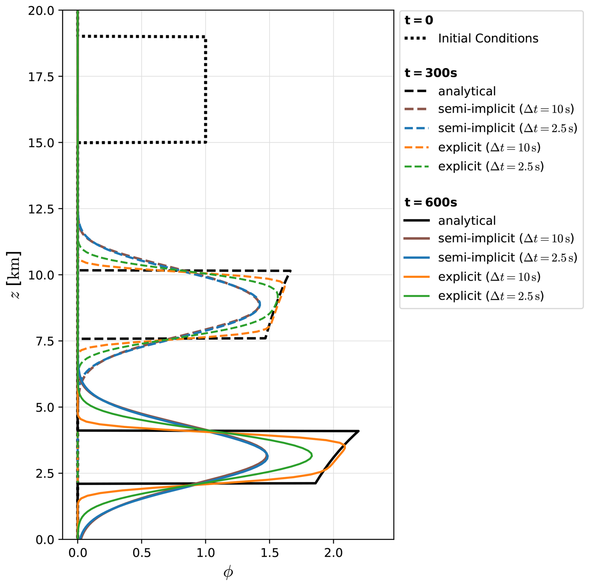
Figure 2 Linear advection, solving Eq. (28) numerically in comparison to the analytical solution. The solutions for Δz=100 m and both time steps Δt=10 s and Δt=2.5 s are shown. For the explicit scheme, the case with Δt=2.5 s would be equivalent to using Δt=10 s and four substeps, since no other physics are applied in-between the sedimentation steps in this experiment. For the semi-implicit scheme, the solutions for both time steps Δt=10 s and Δt=2.5 s overlap and are almost identical.

3.2 Sedimentation in the two-moment scheme

When considering sedimentation in the two-moment scheme, the numerical solutions of Eq. (9) should best be compared against a direct solution of the original spectral budget equation, Eq. (1). We compute such a reference by combining a bin method with analytical solutions of the linear advection equation: First, the initial conditions are decomposed into spectral components, i.e., 10 000 equally spaced mass bins, such that (at least) 99.9 % of all particles are inside the region that is covered by the bins. Following that, each bin's respective number density is advected using an analytical solution of the linear advection equation with velocities given by Eq. (6). The number distribution obtained from those advected bins is then used to determine the first two moments and reflectivity for comparison with the numerical two-moment scheme solutions.

In realistic numerical weather prediction (NWP) model setups, Δz spans approximately two orders of magnitude, e.g., from 20 m at the lowest levels to over 1 km at z≈20 km. Considering that, and anticipating future resolution increases (also in the vertical) in accordance with rising computing power, it is important to understand how the vertical mesh resolution impacts the sedimentation schemes. For investigating that, we compare numerical solutions obtained from a wide range of vertical resolutions, closely resembling a convergence study apart from comparing against the spectral solution that clearly differs from the numerical solutions in the limit $\mathrm{\Delta }z,\mathrm{\Delta }t\to \mathrm{0}$.

In more detail, we use the numerical schemes as defined in Sect. 2, except for neglecting all hydrometeor interactions, i.e., 𝒬_CCN and 𝒬^Δt from Eq. (27) are skipped. The initial conditions, consisting of three square peaks and a small nonzero background hydrometeor concentration, are chosen to be exactly representable on the vertical grid of all resolutions. The time step is selected to be sufficiently small to avoid frequent Lipschitz condition violations (to avoid introducing spurious oscillation in the explicit scheme), and is simultaneously refined with Δz, i.e., $\mathrm{\Delta }z/\mathrm{\Delta }t=\mathrm{12}$ m s⁻¹ is held constant. Further, ρ≡ρ₀ is assumed everywhere, and ICON's hail hydrometeor parameters are used as listed in Table 2. Figure 3 depicts hydrometeor profiles from this setup, showing initial conditions, a spectral reference solution, and hydrometeor profiles for three mesh resolutions and numerical configurations. The agreement between numerical and spectral solutions is evaluated using the standard L¹ norm, and drawn as a function of mesh resolution in Fig. 4.

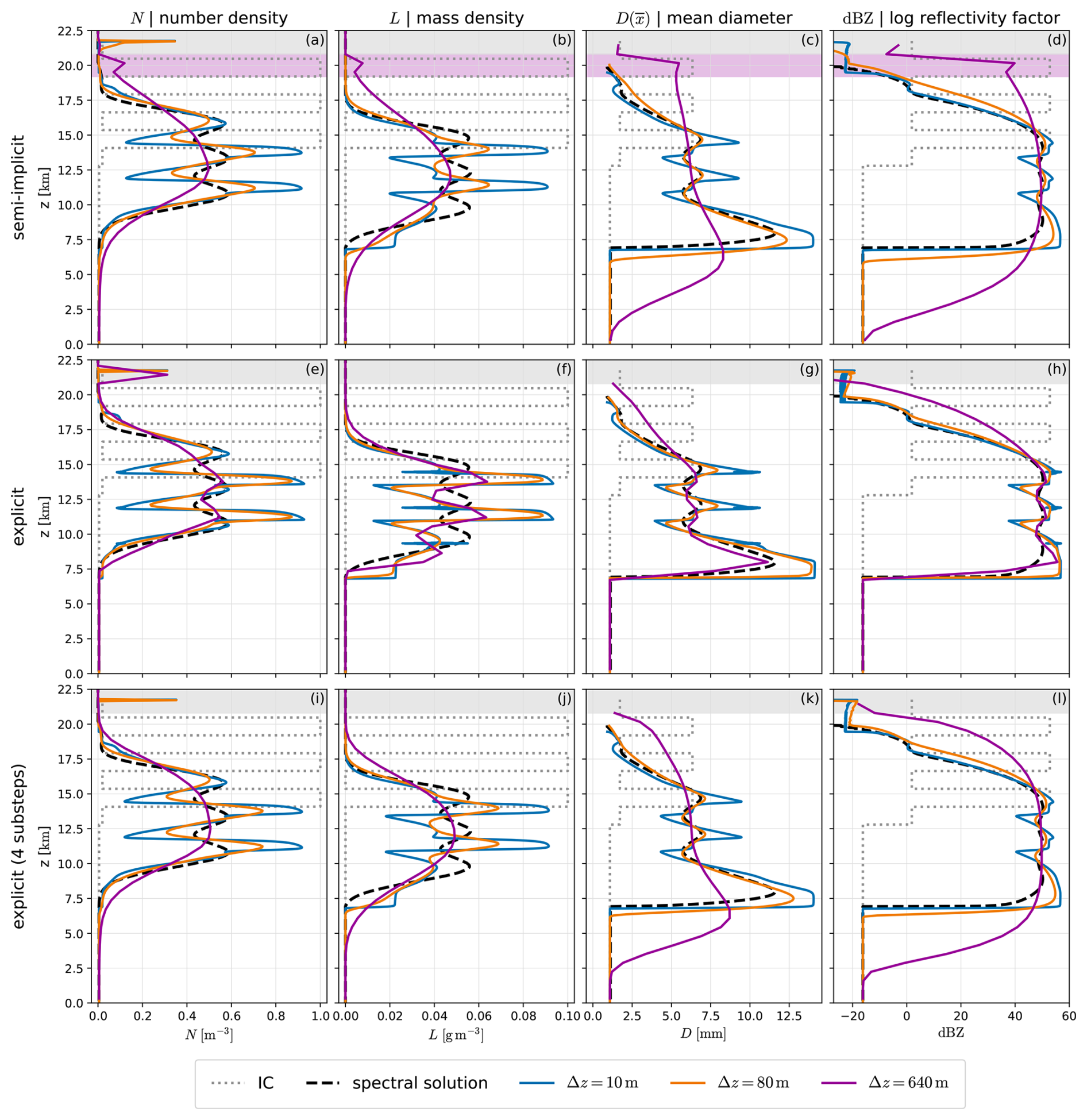
Figure 3 Hydrometeor profiles (N, L, diagnostic mean diameter, reflectivity) in a pure sedimentation case after t_end≈534 s, for three different mesh resolutions and numerical schemes, in addition to the reference spectral solution. The diameter is only drawn where $L>q_{\text{crit}}={\mathrm{10}}^{-\mathrm{9}}$ kg m⁻³. In the area shaded gray, spikes induced by the operator 𝒟, defined in Eq. (27), are visible. The region shaded purple highlights numerical artifacts caused by the flux limiter defined in Eq. (13). Setup details are provided in Sect. 3.2.

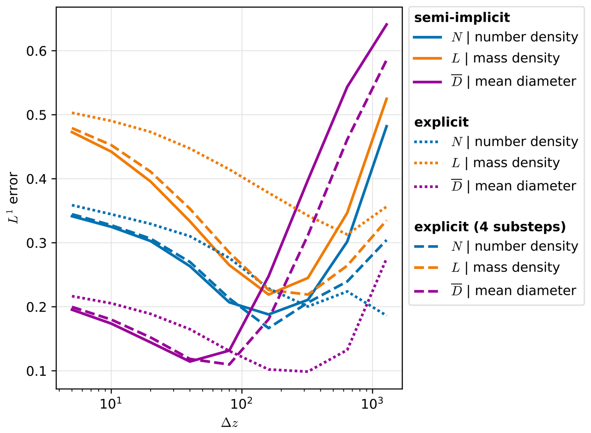
Figure 4 L¹ errors of N, L and diagnostic mean diameter are shown, computed using the numerical schemes in comparison to the spectral solution after a fixed time t_end≈534 s, for spatial resolutions $\mathrm{\Delta }z=\mathrm{5},\mathrm{10},\mathrm{20},\mathrm{40},\mathrm{\dots },\mathrm{1280}$ m. For the mean diameter, only cells where $L>{\mathrm{10}}^{-\mathrm{9}}$ kg m⁻³ in both spectral and numerical solutions are considered. Setup details are provided in Sect. 3.2.

For the semi-implicit scheme, very high resolution prevents the decay of the structure imposed by the initial conditions, and even generates new extrema. Medium resolutions, roughly of the order Δz≈100 m, minimize the discrepancy, although notably, the lowest errors in number and mass densities do not perfectly correspond to the lowest diameter errors. On the contrary, very low resolutions produce overly smooth features, again resulting in large errors. Furthermore, the excessive smoothing also spreads mass to outside the regions where most mass is located in the spectral solution, which would translate to a too early and too late onset and end, respectively, of precipitation on the ground. In those leading and trailing edges of the precipitation column, considerable diameter anomalies can also be observed in Fig. 3. Considering the reflectivities in Fig. 3, the solutions with very low resolution result in a maximum reflectivity close to the spectral solution but a too large vertical spread, whereas higher resolutions produce too high reflectivity maxima at the leading edge.

As the explicit scheme is substantially less diffusive, the mesh resolution that minimizes the discrepancy to the spectral solution is significantly shifted towards coarser resolutions of Δz≈500 m without substepping, whereas the diffusion introduced by substepping results in behavior very comparable to the semi-implicit method.

In some configurations, the profiles depicted in Fig. 3 exhibit unexpected spikes in the upper domain region, as indicated by the shaded areas. For the number density, the spikes that are shaded gray, arise from the source term's operator 𝒟, as defined in Eq. (27). This operator determines the number density based on an assumed particle size distribution when it drops below a threshold. In the configuration shown in Fig. 3 with hail, this is an exponential distribution with respect to the diameter, leading to a sharp increase of N. However, in the semi-implicit scheme, the mass density also displays a spike in the upper domain region, clearly visible in the case Δz=640 m in the region highlighted in purple. We can conclusively identify the semi-implicit scheme's restrictive flux limiter, cf. Eq. (13), as the culprit; and here, the effect is further enhanced by the explicit velocity approximation from Eq. (12) which also reduces the sedimentation speed at the highest level where L>q_crit due to the velocity cutoff by q_crit in Eq. (26). Additionally, in the locations where those flux limiter artifacts show up, even an increase of the mean diameter with height can be observed, which is clearly unphysical as size sorting should produce the opposite effect. In the analysis of case studies, which follows next, we will also investigate the presence of those flux limiter artifacts.

4 Case studies

Finally, the sedimentation schemes will be examined in full ICON simulations of six individual summer days (listed in Fig. 6) with significant convective activity. We employ a domain encompassing Switzerland, with 1 km horizontal resolution and 80 vertical levels, ranging from Δz₈₀≈20 m near the ground to Δz₁≈2 km in the domain's highest level, terminating at 22 km height, and the main model time step Δt=10 s. Simulations were performed from 00:00–22:00 UTC of six distinct days with severe thunderstorms, using COSMO analysis states for initial and lateral boundary conditions. For investigating the sedimentation schemes, we focus on severe precipitation events such as thunderstorms, particularly including graupel and hail. Therefore, we focus on analyzing the time period from 14:00–20:00 UTC, approximately when the highest density of thunderstorms and precipitation is observed (Dai, 2001; Feldmann et al., 2021).

Since the sedimentation schemes mainly differ in the source term treatment (predictor-corrector or sequential) and the extent of numerical diffusion (explicit is much less diffusive), these two differences are investigated separately by comparing both source term methods in the semi-implicit scheme, and varying the amount of numerical diffusion in the explicit scheme by applying substepping. Furthermore, we also try the semi-implicit scheme with our proposed flux limiter improvement given in Eq. (14); all five configurations are summarized in Table 4.

Table 4 The five sedimentation scheme configurations used in the full ICON simulations. We differentiate between the semi-implicit (IM) and explicit (EX) schemes, predictor-corrector (pc) and sequential (seq) source term treatment, sedimentation substepping (sub) and the flux limiter improvement (lim) from Eq. (14). The default configuration is IM_pc, and it is possible to switch to the EX_seq version via ICON's namelist parameters. All other configurations currently require small modifications to the source code, such as changing hard-coded switches.

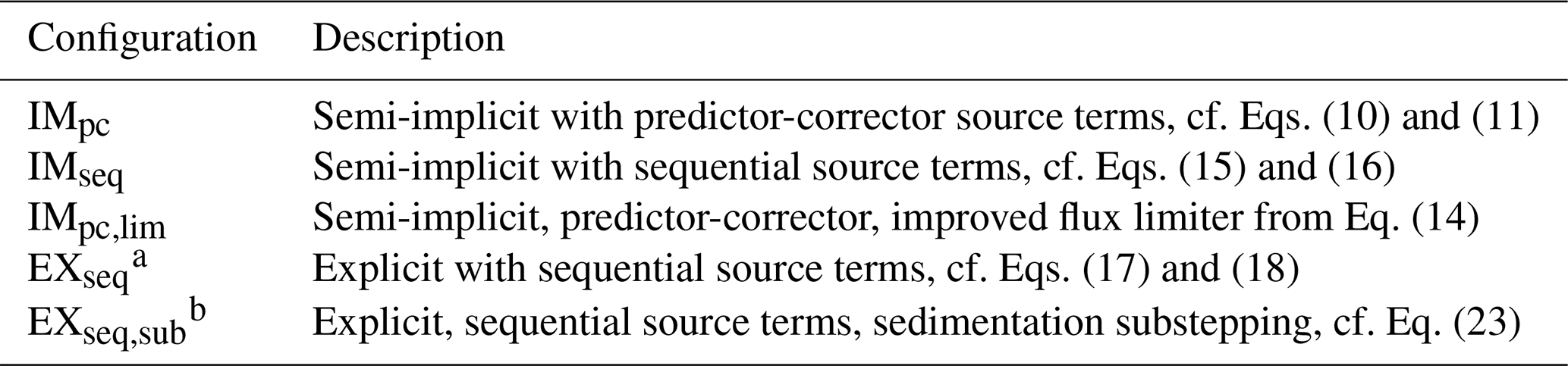
^a In this configuration, the numerical sedimentation scheme is significantly less diffusive compared to the rest.
^b The number of substeps N_sub, cf. Eq. (23), is 11 (rain), 41 (graupel), and 16 (hail) for our grid.

4.1 Precipitation and radar reflectivity

We start by providing a map view of the 20 July 2022 case in Fig. 5, where we compare precipitation and radar reflectivity of the IM_pc, IM_seq, and EX_seq configurations (the IM_pc,lim and EX_seq,sub configurations are provided in Fig. C1). On this day, several thunderstorms with large hail were observed over the Jura mountains at the France–Switzerland border, around Basel, and the Prealps from Bern to Zug (https://www.sturmarchiv.ch/index.php?title=Extremereignisse_2022#Juli, last access: 6 November 2025). Although slightly different in detail, all configurations predict storms over the Jura mountains (in the northwest in Fig. 5a–c), and in a diagonal band from the southwest to the northeast of Switzerland. In a zoom-in view of a single storm, the 1 h accumulated hail is shown in Fig. 5d–f. Both configurations with sequential source term treatment (IM_seq, EX_seq) result in higher maxima of accumulated hail compared to the predictor-corrector variant IM_pc. This is not a truncation effect of the time window, as most precipiation occurs in the window's center at around 17:00 UTC. In addition, the storm's track is slightly shifted south in the EX_seq case. Next, we show the radar reflectivity at 2 km height at time 17:00 UTC in Fig. 5g–i, and the corresponding instantaneous precipitation rate in Fig. 5j–l. Notably, all three configurations exhibit a similar U-shaped structure. Finally, for a few select grid points, we show how the precipitation rate evolves during a 15 min window in Fig. 5m–o. All configurations exhibit precipitation rates in excess of 300 mm h⁻¹, however only for a few minutes as the storm moves and eventually dissipates; e.g., on average 300 mm h⁻¹ for 5 min results in 25 mm of precipitation on the ground. However, particularly for the EX_seq configuration, the precipitation rate appears less smooth, i.e., includes small oscillations at various points, with steeper gradients and more rapid changes compared to the default implicit variant IM_pc.

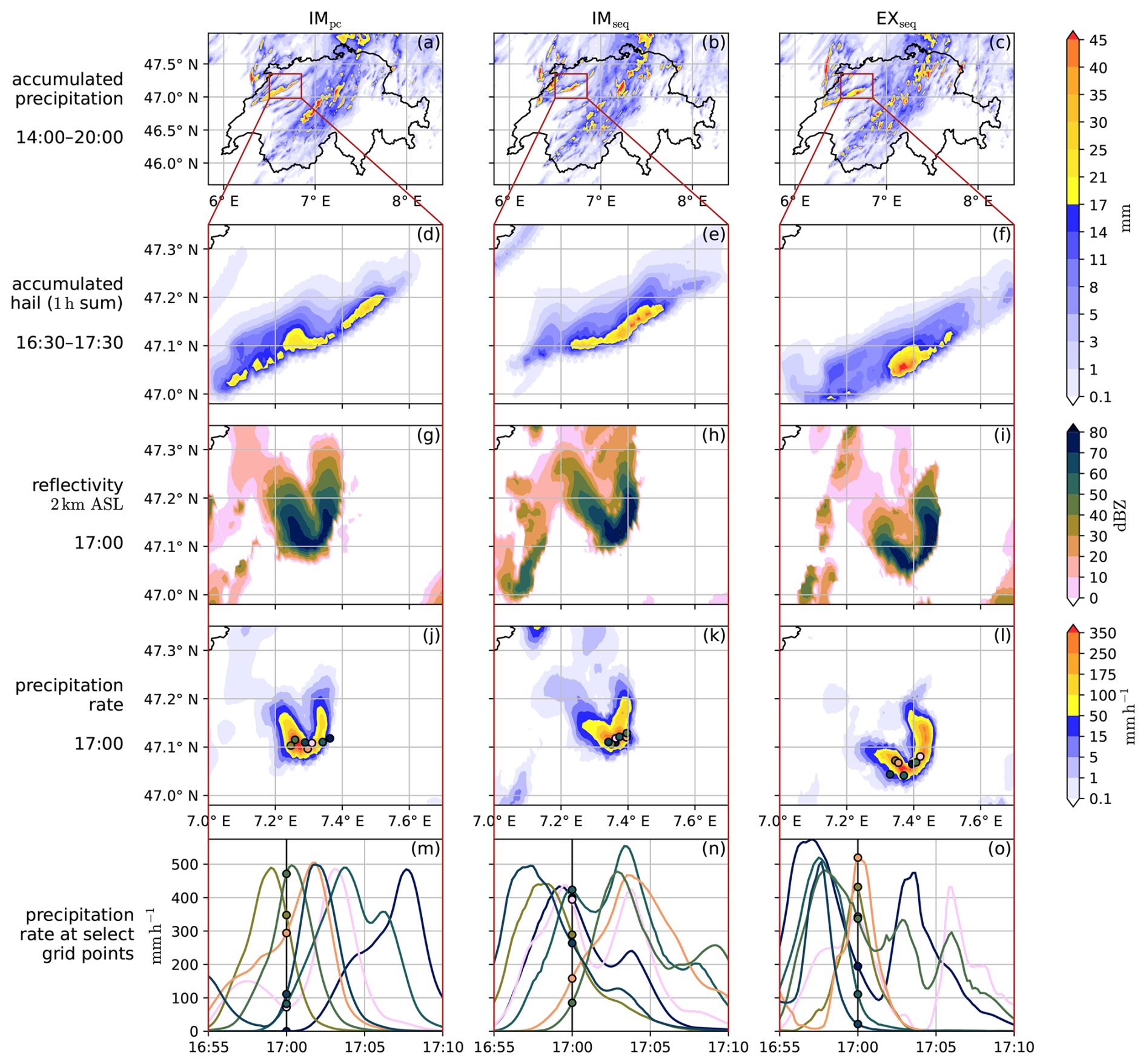
Figure 5 For the 20 July 2022 case and the IM_pc, IM_seq, and EX_seq configurations, the accumulated precipitation from 14:00–20:00 UTC over the entire simulation domain is shown in the first row (a–c). The following rows give a zoom–in view of a severe storm over the Jura mountains, specifically the 1 h accumulated hail (d–f), radar reflectivity at 2 km a.s.l. (g–i), and instantaneous precipitation rate at 17:00 UTC (j–l). The last row (m–o) displays the time evolution of precipitation rates for a few select grid points whose locations are marked in the row (j–l) above. The configurations IM_pc,lim and EX_seq,sub are shown in Fig. C1.

Notably, out of the five configurations listed in Table 4, the storm cell shown in Fig. 5d–o deviates significantly only in the configuration with the improved flux limiter IM_pc,lim (Fig. C1), where it produces less intense precipitation and hail, and lacks the U–shaped structure. We suspect this discrepancy is largely coincidental, since inspecting other storm cells reveals that different configurations occasionally exhibit similar outliers. As the flux limiter improvement is only a minor numerical adjustment, this deviation may rather originate from the inherent sensitivity of such individual convective cells after 17 h of lead time. Especially in the context of this broader meteorological forecast uncertainty, the other configurations produce remarkably similar outcomes. Still, we clearly see differences in the roughness of precipitation rates, and the accumulated hail may hint at slight shifts in the precipitation (rate) distribution, and/or the ratio between hydrometeor classes.

4.2 Precipitation rate roughness

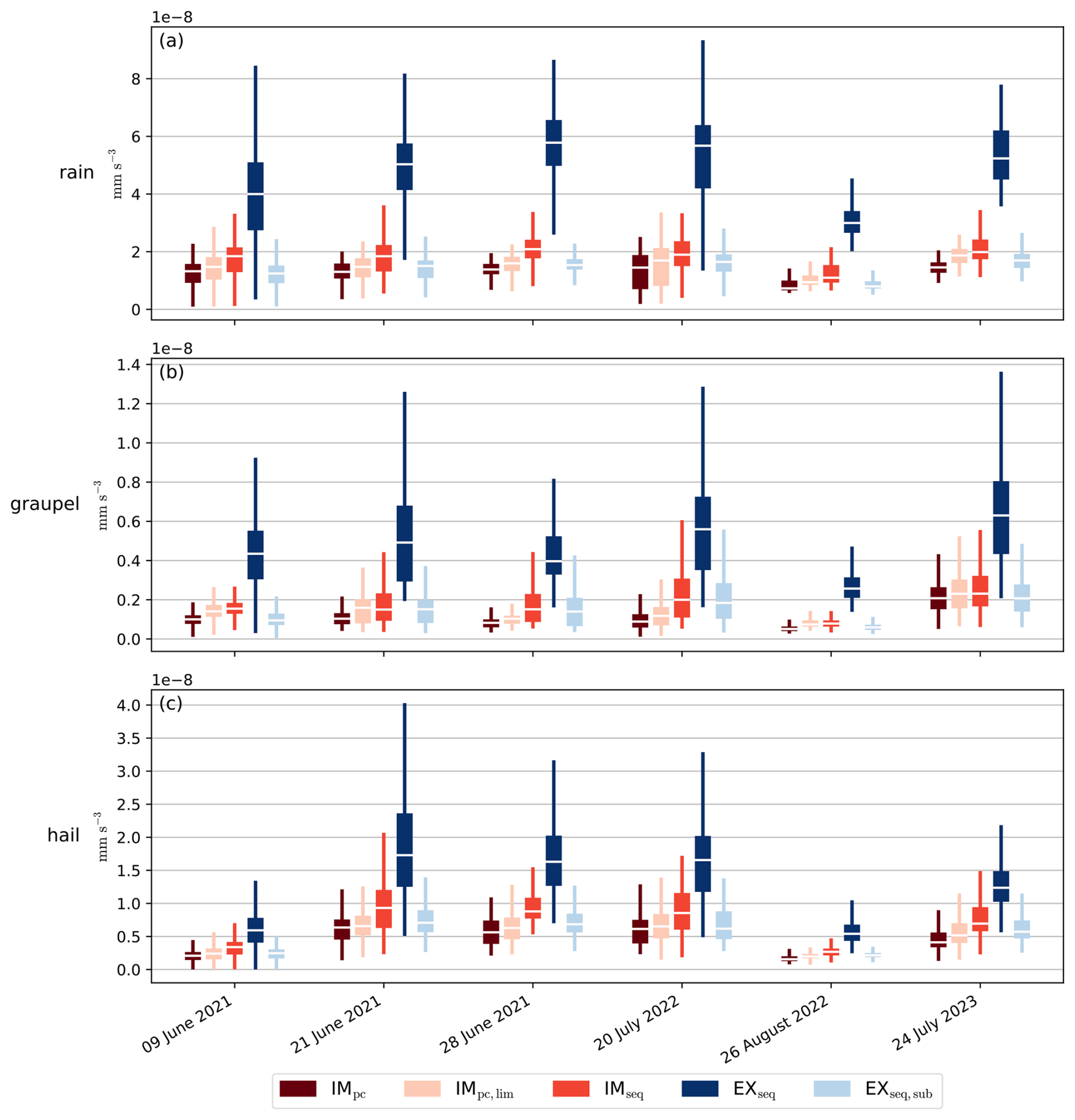
Due to the varying amounts of numerical diffusion in the sedimentation schemes, the vertical hydrometeor profiles are expected to vary in smoothness, possibly amplified by instability-like oscillations from Lipschitz condition violations in the explicit scheme. As the downward movement of the three-dimensional hydrometeor fields effectively transforms the vertical structure into a temporal signal on the ground, we will simply investigate the precipitation rates. Specifically, we define the mean precipitation rate roughness R(t_n) at some time t_n as the spatial mean of absolute temporal second derivatives of instantaneous precipitation rates r_i, using a finite difference approximation:

$$\begin{array}{}\text{(29)}& R\left(t_n\right):={\displaystyle \frac{\mathrm{1}}{N_{\text{cells}}}}\sum _{i=\mathrm{1}}^{N_{\text{cells}}}\left|{\displaystyle \frac{r_i^{(n-\mathrm{1})}-\mathrm{2}{r}_i^{\left(n\right)}+r_i^{(n+\mathrm{1})}}{\mathrm{\Delta }{t}^{\mathrm{2}}}}\right|.\end{array}$$

Figure 6 shows this mean roughness for all six cases, split into rain, graupel, and hail classes. In all cases, the mean roughness of both rain and graupel is more than twice as high using the default explicit scheme in comparison to the other configurations; for hail the behavior is similar, just slightly less pronounced. Considering the semi-implicit versions, the roughness seems to increase very little when switching from predictor-corrector to sequential source term treatment, thus confirming that the large roughness increase of the default explicit scheme is not caused by the source terms. Furthermore, the explicit variant with substepping closely resembles the semi-implicit methods, as expected due to the relaxed Lipschitz condition and more numerical diffusion compared to the default case. Also, the improved flux limiter for the semi-implicit scheme performs very similarly to the default case, possibly with a very slight roughness increase. This would not be surprising, as the improved flux limiter no longer tends to artificially delay (and thus smooth) the trailing edge of precipitation columns, i.e., could allow for more rapid ends of precipitation events.

Figure 6 Mean precipitation rate roughness R(t_n) from Eq. (29), over the time period 14:00–20:00 UTC. The corresponding time series are provided by Fig. C2.

4.3 Precipitation rate extrema

If the explicit scheme's less smooth instantaneous precipitation rates were caused by the frequent presence of severe shocks or spurious oscillations, it would be reasonable to expect a correspondingly increased occurrence of extreme precipitation events. Thus, we determine three high percentiles (99th, 99.9th, 99.99th) of the instantaneous precipitation rates in the reference default semi-implicit sedimentation scheme, and then compare how often the other configurations' precipitation rates exceed those thresholds across the domain from 14:00–20:00 UTC, separately for hail, graupel, rain and combined precipitation rates in all six cases.

Figure 7 displays those precipitation rate statistics, in addition to the (relative) mean rates. The default explicit scheme EX_seq shows increased mean hail rates in all six cases while reducing the mean graupel rate in five out of six. Interestingly, all other configurations that also apply the source terms sequentially (IM_seq, EX_seq,sub) exhibit the very same behavior, while the IM_pc,lim configuration shows no clear deviations from the reference. This clearly indicates that those shifts are caused by the source term treatment as opposed to numerical diffusion differences or spurious oscillations and shocks. For mean rain and combined precipitation rates, all configurations perform relatively similar. Analogous observations can be made for extreme hail and graupel rate events, which occur more and less frequently, respectively, when using the sequential source term treatment. In the 99.9th and 99.99th percentiles, we can further observe slightly higher values in configurations with sequential source term treatment, while the flux limiter improvement shows no effect again. In summary, all clear trends in the precipitation rate distribution actually result from the different source term treatment rather than instabilities, shocks or reduced numerical diffusion.

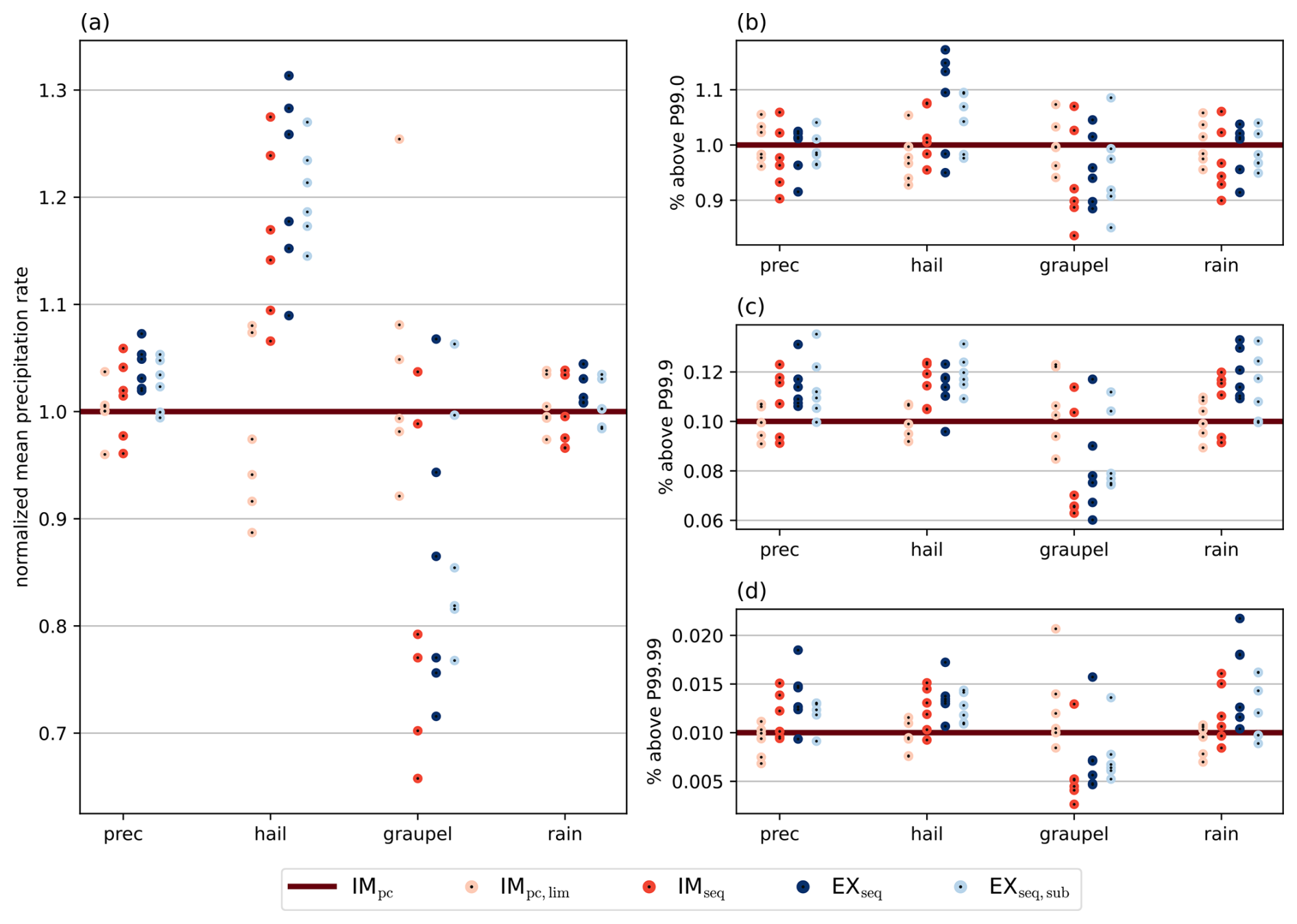
Figure 7 Precipitation rate statistics from 14:00–20:00 UTC for all six cases and the five microphysics configurations from Table 4, using the default semi-implicit scheme as reference. (a) Mean precipitation rates across the space–time domain, normalized by the reference. (b–d) How often the (b) 99th, (c) 99.9th, (d) 99.99th percentiles of the reference are exceeded across the space–time domain.

Determining why such clear shift from graupel to hail occurs when employing the sequential source term treatment is challenging to explain, especially as there are many pathways to obtain such results. In the sequential treatment, the source terms are integrated with the explicit Euler method, as shown in Eqs. (15) and (17), just before the sedimentation step. Inside the source term computation, the individual microphysical processes are again split sequentially, cf. Eq. (27), also introducing significant splitting errors as discussed by Barrett et al. (2019). Given the fast nature of those microphysical processes, mechanisms creating or growing hail hydrometeors may overshoot, potentially exacerbated by the explicit Euler integration. For example, overshoots in the graupel–hail conversion in wet growth regime would directly lead to the observed effect, especially as no reverse pathway exists because melting does not reduce the hail's bulk density which would warrant such a process (Blahak, 2008). Similarly, the specific ordering of riming processes may amplify hail production, since hail riming is applied before graupel riming.

In contrast, the predictor-corrector treatment integrates source terms within the Crank-Nicolson sedimentation step, as shown in Eq. (11). In this context, the method can be understood as the approximation $\mathrm{0.5}\cdot \left(Q\right({\mathit{\varphi }}_k^{\left(n\right)})+Q({\mathit{\varphi }}_k^{(n+\mathrm{1})}\left)\right)\approx Q\left({\mathit{\varphi }}_k^{*}\right)$ for the time-averaged source term. As ${\mathit{\varphi }}_k^{*}$, given by Eq. (10), already encompasses the source term update of all upstream levels and sedimentation, $Q\left({\mathit{\varphi }}_k^{*}\right)$ can also be considered a semi-implicit approximation, at least with respect to the upstream levels' contributions. Conversely, in the limit of zero velocity (v→0), the predictor-corrector and sequential variants are even identical. For fast sedimentation velocities, the share of those implicitly considered contributions thus rises, which may slightly weaken or reduce overshoots of some processes, e.g., the graupel–hail conversion. However, like in the sequential treatment, the individual microphysical processes inside the source term computation are still split sequentially, introducing aforementioned splitting errors. For fast hydrometeors, which repeatedly encounter the source terms (the “implicit contributions”) in a single time step, those errors may be smaller or manifest differently compared to the sequential splitting of source terms and sedimentation.

For high sedimentation speeds, particularly C≫1, the sequential source term treatment suffers from another issue, as it is theoretically possible that some rapidly sedimenting particles fall through thin layers without capturing any interactions, if their positions never actually line up at any time point t⁽ⁿ⁾. Conversely, when positions do line up, interactions may be locally overestimated, since the rapidly falling particles do not actually spend the entire time step in the interaction layer as assumed in the source term computation. Such layer alignment effects may average out or even induce vertical oscillations, depending on the level of diffusion. In contrast, such problems cannot arise with the predictor-corrector method. In practice, however, we are only able to reproduce such missing hydrometeor interactions in idealized experiments with the default explicit scheme, since the extensive numerical diffusion of all other configurations inevitably leads to some interaction. Furthermore, we find that whether a specific process is appropriately captured, or under- or overestimated also heavily depends on its timescale, the sedimentation speed and geometry of the interacting layers, which is also influenced by numerical diffusion. Since many parameters were tuned using the default semi-implicit predictor-corrector configuration for achieving better overall skill scores, we suspect those parameters are also inevitably linked to the discretization and splitting errors of this specific model configuration (and resolution), with unclear sensitivities or impacts to changes in the numerical schemes.

4.4 Flux limiter artifacts

As we have shown in Sect. 3, the semi-implicit method's current flux limiter is too restrictive, artificially delaying sedimentation of a precipitation column's trailing edge. When used in a two-moment scheme, this even resulted in an unphysical mean diameter increase in those regions, i.e., produced an effect opposite the expected gravitational sorting. Next, we will examine if those flux limiter artifacts translate to the full ICON simulations or turn out to be irrelevant or masked, e.g., by the source terms' operator 𝒟 from Eq. (27).

To identify the upper edge of precipitation columns, we make use of the mass density threshold q_crit, used in Eq. (26) to determine whether non-negligible mass for sedimentation is present in a cell: Only if the mass density exceeds this threshold, a nonzero sedimentation speed is applied. In each column, the highest cell with L>q_crit is identified, if it exists, and the mean height of all those cells determined. In Fig. 8, we show the difference of those mean heights compared to the default semi-implicit scheme.

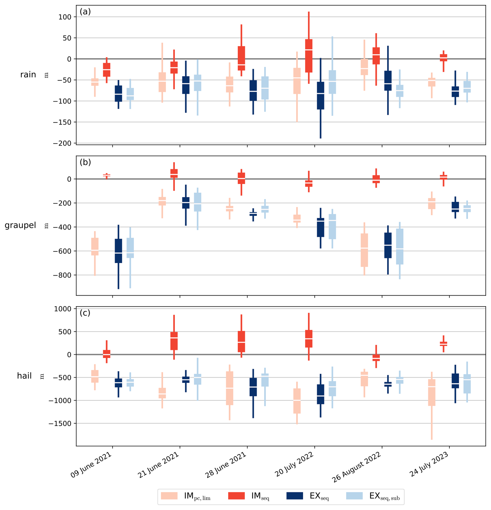
Figure 8 Difference of the mean upper q_crit threshold height (i.e., the spatial mean of the highest level's height with $L>q_{\text{crit}}={\mathrm{10}}^{-\mathrm{9}}$ kg m⁻³, over the columns where such threshold exists), to the default semi-implicit scheme IM_pc; for the time period 14:00–20:00 UTC with 10 min sampling interval. The value of q_crit is motivated by its use in Eq. (26); a similar analysis using a larger threshold is provided with Fig. C3.

For all three hydrometeor classes (rain, graupel, hail), the IM_seq configuration shows almost no difference in the q_crit threshold height compared to the default semi-implicit version, except for a slight increase for hail in some cases. Such close agreement indicates that the method to integrate the source terms does not considerably impact this threshold's height, and is expected since both configurations make use of the too restrictive flux limiter given in Eq. (13). Next, the IM_pc,lim configuration results in consistently lower q_crit threshold heights, most pronounced for hail and graupel, but also clearly visible for rain. Again, this is expected due to the improved flux limiter, which no longer artificially slows sedimentation on a precipitation columns' trailing edge. Furthermore the IM_pc,lim variant performs very similarly to both explicit configurations, which do not suffer from an excessively restrictive limiter. This further confirms that the source term method is irrelevant for this metric, and also strongly suggests that the amount of numerical diffusion is irrelevant as well here. Therefore, the improved flux limiter increases similarity between the two sedimentation schemes' behaviors by eliminating a purely numerical artifact.

5 Summary and conclusions

We provided a concise and detailed description of the numerical methods and their configuration options employed in ICON's two-moment microphysics module. Since the bulk sedimentation description does not fully capture the original spectral sedimentation equation, e.g., it erroneously produces shock waves, those numerical schemes are deliberately chosen to be very diffusive to compensate. Since the numerical diffusion is not parameterized, its amount heavily depends on the time step, vertical resolution and specific scheme in question; particularly we have shown that the semi-implicit sedimentation scheme is more diffusive than the explicit version. In an idealized setup with pure sedimentation, we observed that too much diffusion leads to reduced size sorting, whereas too little diffusion produces excessive size sorting and reduces the capacity to eliminate the spurious shocks introduced by the bulk velocity approximations.

The standard semi-implicit sedimentation scheme is coupled to the microphysical source terms with a predictor-corrector method, resulting in a partially implicit integration of the source terms which is very time-consuming on GPUs in its current form. Moreover, we never encountered any stability issues despite an explicit approximation for some velocities, which works almost surprisingly well. However, we discovered and proposed a solution to a purely numerical artifact caused by a too restrictive flux limiter, leading to artificially delayed sedimentation (and inconsistent size sorting) in trailing edges of hydrometeor columns. In contrast, the explicit scheme employs a simple sequential time-splitting for coupling to the source terms, which are just explicitly integrated before the sedimentation step. For hydrometeors with high sedimentation speeds, the splitting and discretization errors differ compared to the predictor-corrector method, although exact details vary depending on many factors such as the timescale of individual processes, sedimentation speeds, the geometry of interacting layers, and numerical diffusion.

In case studies, we have observed significantly rougher instantaneous precipitation rates for the explicit scheme, which directly translates to more jagged patterns in the three-dimensional hydrometeor profiles, likely caused by a combination of factors (reduced numerical diffusion, Lipschitz condition violations). Conversely, changes in the precipitation rate distribution, particularly a shift from graupel to hail, are induced by the different source term treatment. Although in idealized experiments with pure sedimentation, stability of the explicit scheme seems rather fragile in certain cases (oscillations may even appear without violating the Lipschitz condition using high vertical resolutions, and rarely vanish unless they reach the ground), in full model simulations those issues seem to be mitigated by additional diffusive or smoothing operations (tracer advection, source terms). Also, the most problematic high vertical resolutions are only encountered in the lowest levels, which reduces the available time for serious oscillations to develop.

In the future, NWP model resolutions are likely to increase in accordance with available computing power. If only the horizontal resolution is increased, the ensuing time step reduction will lead to more numerical diffusion in the explicit scheme, but leave the semi-implicit scheme largely unaffected. This is noteworthy, as it increases the similarity between the two sedimentation methods, thus rendering the explicit scheme more viable. Conversely, also increasing the vertical resolution results in reduced numerical diffusion for both schemes, which may become problematic for the explicit scheme due to the loss of smoothing capacity for oscillations that are either induced numerically or by the bulk parameterization. Sedimentation substepping, using just a small number of substeps, could serve as effective means to increase the explicit scheme's viability in those cases. In contrast, we do not anticipate comparable issues for the semi-implicit scheme. In all cases, the smaller time step leads to reduced splitting errors in the source terms, which could necessitate small adjustments of tuned parameters.

Given that parameter tuning of the source terms was conducted using the semi-implicit method in predictor-corrector configuration, as currently operational at DWD, GPU performance improvements of the semi-implicit scheme would still be welcome to render it feasible for GPUs. Nevertheless, we find that the explicit scheme can be safely used on GPUs currently, since the differences to the semi-implicit scheme are small in relation to other meteorological forecast uncertainties. In case more numerical diffusion is desired, applying a few substeps or the semi-implicit configuration with sequential source terms constitute suitable alternatives with only modest performance impacts.

Appendix A: Truncation error analysis for the semi-implicit scheme

We aim to derive the first-order error terms, i.e., the errors that are scaling with Δz, Δt, in addition to the mixed term ΔzΔt. For simplicity, only the linear advection equation ${\mathit{\varphi }}_t=-(v\mathit{\varphi }{)}_z$ is considered, although in the most general case where v can vary in both space and time. Although this approach neglects effects that may appear when solving (coupled) quasilinear equations such as Eq. (9), it still provides a good starting point to reason about the scheme's behavior, e.g., by analyzing the diffusive error terms. Even obtaining the truncation errors for a single quasilinear equation, i.e., where v=h(ϕ), should be straightforward; it only requires substituting chain rule-based expressions (e.g., $v_t=h^{\prime }\left(\mathit{\varphi }\right){\mathit{\varphi }}_t$) for the velocity derivatives in the truncation error as derived next.

On a uniform grid Δz_k=Δz, without source terms and flux limiter, the update step of the semi-implicit scheme can easily be obtained from Eq. (11):

$$\begin{array}{}\text{(A1)}& {\displaystyle }\begin{array}{rl}& {\mathit{\varphi }}_k^{(n+\mathrm{1})}={\left(\mathrm{1}-{\displaystyle \frac{\mathrm{\Delta }t}{\mathrm{2}\mathrm{\Delta }z}}{\stackrel{\mathrm{̃}}{v}}_k^{(n+\mathrm{1})}\right)}^{-\mathrm{1}}\\ & \cdot \left[{\mathit{\varphi }}_k^{\left(n\right)}-{\displaystyle \frac{\mathrm{\Delta }t}{\mathrm{2}\mathrm{\Delta }z}}({\stackrel{\mathrm{̃}}{v}}_{k-\mathrm{1}}^{(n+\mathrm{1})}{\mathit{\varphi }}_{k-\mathrm{1}}^{(n+\mathrm{1})}+v_{k-\mathrm{1}}^{\left(n\right)}{\mathit{\varphi }}_{k-\mathrm{1}}^{\left(n\right)}-v_k^{\left(n\right)}{\mathit{\varphi }}_k^{\left(n\right)})\right]\end{array}\text{(A2)}& {\displaystyle }{\stackrel{\mathrm{̃}}{v}}_k^{(n+\mathrm{1})}={\displaystyle \frac{\mathrm{1}}{\mathrm{2}}}(v_k^{\left(n\right)}+v_{k-\mathrm{1}}^{\left(n\right)}).\end{array}$$

Simple algebraic manipulations yield:

$$\begin{array}{}\text{(A3)}& \begin{array}{rl}{\displaystyle \frac{\mathrm{1}}{\mathrm{\Delta }t}}& ({\mathit{\varphi }}_k^{(n+\mathrm{1})}-{\mathit{\varphi }}_k^{\left(n\right)})=\\ & \begin{array}{rl}-{\displaystyle \frac{\mathrm{1}}{\mathrm{2}\mathrm{\Delta }z}}(& v_{k-\mathrm{1}}^{\left(n\right)}{\mathit{\varphi }}_{k-\mathrm{1}}^{\left(n\right)}-v_k^{\left(n\right)}{\mathit{\varphi }}_k^{\left(n\right)}+{\stackrel{\mathrm{̃}}{v}}_{k-\mathrm{1}}^{(n+\mathrm{1})}{\mathit{\varphi }}_{k-\mathrm{1}}^{(n+\mathrm{1})}\\ & -{\stackrel{\mathrm{̃}}{v}}_k^{(n+\mathrm{1})}{\mathit{\varphi }}_k^{(n+\mathrm{1})}).\end{array}\end{array}\end{array}$$

Next, we perform a Taylor series expansion of some smooth exact solution u(z,t) around the point (z_k,t_n). For better readability, we omit the arguments, i.e., simply write u for u(z_k,t_n):

$$\begin{array}{}\text{(A4)}& {\displaystyle }{\mathit{\varphi }}_k^{\left(n\right)}=u\text{(A5)}& {\displaystyle }{\mathit{\varphi }}_k^{(n+\mathrm{1})}=u+\mathrm{\Delta }t{u}_t+{\displaystyle \frac{\mathrm{\Delta }{t}^{\mathrm{2}}}{\mathrm{2}}}{u}_{tt}+\mathcal{O}\left(\mathrm{\Delta }{t}^{\mathrm{3}}\right)\text{(A6)}& {\displaystyle }{\mathit{\varphi }}_{k-\mathrm{1}}^{\left(n\right)}=u+\mathrm{\Delta }z{u}_z+{\displaystyle \frac{\mathrm{\Delta }{z}^{\mathrm{2}}}{\mathrm{2}}}{u}_{zz}+\mathcal{O}\left(\mathrm{\Delta }{z}^{\mathrm{3}}\right)\text{(A7)}& {\displaystyle }\begin{array}{rl}{\mathit{\varphi }}_{k-\mathrm{1}}^{(n+\mathrm{1})}& =u+\mathrm{\Delta }z{u}_z+\mathrm{\Delta }t{u}_t+{\displaystyle \frac{\mathrm{\Delta }{z}^{\mathrm{2}}}{\mathrm{2}}}{u}_{zz}+\mathrm{\Delta }z\mathrm{\Delta }t{u}_{zt}\\ & +{\displaystyle \frac{\mathrm{\Delta }{z}^{\mathrm{2}}\mathrm{\Delta }t}{\mathrm{2}}}{u}_{zzt}+\mathcal{O}(\mathrm{\Delta }{t}^{\mathrm{2}}+\mathrm{\Delta }{z}^{\mathrm{3}}).\end{array}\end{array}$$

The sufficiently smooth advection speed $v(z,t)<\mathrm{0}$ is similarly expanded:

$$\begin{array}{}\text{(A8)}& {\displaystyle }{v}_k^{\left(n\right)}=v\text{(A9)}& {\displaystyle }{v}_{k-\mathrm{1}}^{\left(n\right)}=v+\mathrm{\Delta }z{v}_z+{\displaystyle \frac{\mathrm{\Delta }{z}^{\mathrm{2}}}{\mathrm{2}}}{v}_{zz}+\mathcal{O}\left(\mathrm{\Delta }{z}^{\mathrm{3}}\right)\text{(A10)}& {\displaystyle }{v}_{k-\mathrm{2}}^{\left(n\right)}=v+\mathrm{2}\mathrm{\Delta }z{v}_z+{\displaystyle \frac{\mathrm{4}\mathrm{\Delta }{z}^{\mathrm{2}}}{\mathrm{2}}}{v}_{zz}+\mathcal{O}\left(\mathrm{\Delta }{z}^{\mathrm{3}}\right).\end{array}$$

For ${\stackrel{\mathrm{̃}}{v}}^{(n+\mathrm{1})}$, this results in:

$$\begin{array}{}\text{(A11)}& {\displaystyle }\begin{array}{rl}{\stackrel{\mathrm{̃}}{v}}_k^{(n+\mathrm{1})}& ={\displaystyle \frac{\mathrm{1}}{\mathrm{2}}}(v_k^{\left(n\right)}+v_{k-\mathrm{1}}^{\left(n\right)})\\ & =v+{\displaystyle \frac{\mathrm{\Delta }z}{\mathrm{2}}}{v}_z+{\displaystyle \frac{\mathrm{\Delta }{z}^{\mathrm{2}}}{\mathrm{4}}}{v}_{zz}+\mathcal{O}\left(\mathrm{\Delta }{z}^{\mathrm{3}}\right)\end{array}\text{(A12)}& {\displaystyle }\begin{array}{rl}{\stackrel{\mathrm{̃}}{v}}_{k-\mathrm{1}}^{(n+\mathrm{1})}& ={\displaystyle \frac{\mathrm{1}}{\mathrm{2}}}(v_{k-\mathrm{1}}^{\left(n\right)}+v_{k-\mathrm{2}}^{\left(n\right)})\\ & =v+{\displaystyle \frac{\mathrm{3}}{\mathrm{2}}}\mathrm{\Delta }z{v}_z+{\displaystyle \frac{\mathrm{5}}{\mathrm{4}}}\mathrm{\Delta }{z}^{\mathrm{2}}{v}_{zz}+\mathcal{O}\left(\mathrm{\Delta }{z}^{\mathrm{3}}\right).\end{array}\end{array}$$

Those expansions are now substituted into Eq. (A3). The left-hand side is

$$\begin{array}{}\text{(A13)}& \begin{array}{rl}\text{LHS}& ={\displaystyle \frac{\mathrm{1}}{\mathrm{\Delta }t}}({\mathit{\varphi }}_k^{(n+\mathrm{1})}-{\mathit{\varphi }}_k^{\left(n\right)})\\ & ={\displaystyle \frac{\mathrm{1}}{\mathrm{\Delta }t}}\left(u+\mathrm{\Delta }t{u}_t+{\displaystyle \frac{\mathrm{\Delta }{t}^{\mathrm{2}}}{\mathrm{2}}}{u}_{tt}+\mathcal{O}\left(\mathrm{\Delta }{t}^{\mathrm{3}}\right)-u\right)\\ & =u_t+{\displaystyle \frac{\mathrm{\Delta }t}{\mathrm{2}}}{u}_{tt}+\mathcal{O}\left(\mathrm{\Delta }{t}^{\mathrm{2}}\right).\end{array}\end{array}$$

On the right-hand side, we first determine all the flux terms:

$$\begin{array}{}\text{(A14)}& {\displaystyle }{v}_k^{\left(n\right)}{\mathit{\varphi }}_k^{\left(n\right)}=vu\text{(A15)}& {\displaystyle }\begin{array}{rl}{v}_{k-\mathrm{1}}^{\left(n\right)}{\mathit{\varphi }}_{k-\mathrm{1}}^{\left(n\right)}=& \left(v+\mathrm{\Delta }z{v}_z+{\displaystyle \frac{\mathrm{\Delta }{z}^{\mathrm{2}}}{\mathrm{2}}}{v}_{zz}+\mathcal{O}\left(\mathrm{\Delta }{z}^{\mathrm{3}}\right)\right)\\ & \cdot \left(u+\mathrm{\Delta }z{u}_z+{\displaystyle \frac{\mathrm{\Delta }{z}^{\mathrm{2}}}{\mathrm{2}}}{u}_{zz}+\mathcal{O}\left(\mathrm{\Delta }{z}^{\mathrm{3}}\right)\right)\\ =& vu+\mathrm{\Delta }zv{u}_z+{\displaystyle \frac{\mathrm{\Delta }{z}^{\mathrm{2}}}{\mathrm{2}}}v{u}_{zz}+\mathrm{\Delta }z{v}_{z}u\\ & +\mathrm{\Delta }{z}^{\mathrm{2}}{v}_z{u}_z+{\displaystyle \frac{\mathrm{\Delta }{z}^{\mathrm{2}}}{\mathrm{2}}}{v}_{zz}u+\mathcal{O}\left(\mathrm{\Delta }{z}^{\mathrm{3}}\right)\end{array}\text{(A16)}& {\displaystyle }\begin{array}{rl}{\stackrel{\mathrm{̃}}{v}}_k^{(n+\mathrm{1})}{\mathit{\varphi }}_k^{(n+\mathrm{1})}=& \left(v+{\displaystyle \frac{\mathrm{\Delta }z}{\mathrm{2}}}{v}_z+{\displaystyle \frac{\mathrm{\Delta }{z}^{\mathrm{2}}}{\mathrm{4}}}{v}_{zz}+\mathcal{O}\left(\mathrm{\Delta }{z}^{\mathrm{3}}\right)\right)\\ & \cdot (u+\mathrm{\Delta }t{u}_t+\mathcal{O}(\mathrm{\Delta }{t}^{\mathrm{2}}\left)\right)\\ =& vu+\mathrm{\Delta }tv{u}_t+{\displaystyle \frac{\mathrm{\Delta }z}{\mathrm{2}}}{v}_{z}u+{\displaystyle \frac{\mathrm{\Delta }z\mathrm{\Delta }t}{\mathrm{2}}}{v}_z{u}_t\\ & +{\displaystyle \frac{\mathrm{\Delta }{z}^{\mathrm{2}}}{\mathrm{4}}}{v}_{zz}u+{\displaystyle \frac{\mathrm{\Delta }{z}^{\mathrm{2}}}{\mathrm{4}}}\mathrm{\Delta }t{v}_{zz}{u}_t\\ & +\mathcal{O}(\mathrm{\Delta }{z}^{\mathrm{3}}+\mathrm{\Delta }{t}^{\mathrm{2}})\end{array}\end{array}$$

$$\begin{array}{}\text{(A17)}& {\displaystyle }\begin{array}{rl}{\stackrel{\mathrm{̃}}{v}}_{k-\mathrm{1}}^{(n+\mathrm{1})}{\mathit{\varphi }}_{k-\mathrm{1}}^{(n+\mathrm{1})}=& \left(v+{\displaystyle \frac{\mathrm{3}}{\mathrm{2}}}\mathrm{\Delta }z{v}_z+{\displaystyle \frac{\mathrm{5}}{\mathrm{4}}}\mathrm{\Delta }{z}^{\mathrm{2}}{v}_{zz}+\mathcal{O}\left(\mathrm{\Delta }{z}^{\mathrm{3}}\right)\right)\\ & \cdot (u+\mathrm{\Delta }z{u}_z+\mathrm{\Delta }t{u}_t+{\displaystyle \frac{\mathrm{\Delta }{z}^{\mathrm{2}}}{\mathrm{2}}}{u}_{zz}+\mathrm{\Delta }z\mathrm{\Delta }t{u}_{zt}\\ & +{\displaystyle \frac{\mathrm{\Delta }{z}^{\mathrm{2}}\mathrm{\Delta }t}{\mathrm{2}}}{u}_{zzt}+\mathcal{O}(\mathrm{\Delta }{t}^{\mathrm{2}}+\mathrm{\Delta }{z}^{\mathrm{3}}))\\ =& vu+\mathrm{\Delta }zv{u}_z+\mathrm{\Delta }tv{u}_t+{\displaystyle \frac{\mathrm{\Delta }{z}^{\mathrm{2}}}{\mathrm{2}}}v{u}_{zz}\\ & +\mathrm{\Delta }z\mathrm{\Delta }tv{u}_{zt}+{\displaystyle \frac{\mathrm{\Delta }{z}^{\mathrm{2}}\mathrm{\Delta }t}{\mathrm{2}}}v{u}_{zzt}+{\displaystyle \frac{\mathrm{3}}{\mathrm{2}}}\mathrm{\Delta }z{v}_{z}u\\ & +{\displaystyle \frac{\mathrm{3}}{\mathrm{2}}}\mathrm{\Delta }{z}^{\mathrm{2}}{v}_z{u}_z+{\displaystyle \frac{\mathrm{3}}{\mathrm{2}}}\mathrm{\Delta }z\mathrm{\Delta }t{v}_z{u}_t\\ & +{\displaystyle \frac{\mathrm{3}}{\mathrm{2}}}\mathrm{\Delta }{z}^{\mathrm{2}}\mathrm{\Delta }t{v}_z{u}_{zt}+{\displaystyle \frac{\mathrm{5}}{\mathrm{4}}}\mathrm{\Delta }{z}^{\mathrm{2}}{v}_{zz}u\\ & +{\displaystyle \frac{\mathrm{5}}{\mathrm{4}}}\mathrm{\Delta }{z}^{\mathrm{2}}\mathrm{\Delta }t{v}_{zz}{u}_t+\mathcal{O}(\mathrm{\Delta }{t}^{\mathrm{2}}+\mathrm{\Delta }{z}^{\mathrm{3}}).\end{array}\end{array}$$

When computing the flux differences, several terms cancel:

$$\begin{array}{}\text{(A18)}& {\displaystyle }\begin{array}{rl}{v}_{k-\mathrm{1}}^{\left(n\right)}& {\mathit{\varphi }}_{k-\mathrm{1}}^{\left(n\right)}-v_k^{\left(n\right)}{\mathit{\varphi }}_k^{\left(n\right)}=\mathrm{\Delta }zv{u}_z+\mathrm{\Delta }z{v}_{z}u+{\displaystyle \frac{\mathrm{\Delta }{z}^{\mathrm{2}}}{\mathrm{2}}}v{u}_{zz}\\ & +\mathrm{\Delta }{z}^{\mathrm{2}}{v}_z{u}_z+{\displaystyle \frac{\mathrm{\Delta }{z}^{\mathrm{2}}}{\mathrm{2}}}{v}_{zz}u+\mathcal{O}\left(\mathrm{\Delta }{z}^{\mathrm{3}}\right)\end{array}\text{(A19)}& {\displaystyle }\begin{array}{rl}{\stackrel{\mathrm{̃}}{v}}_{k-\mathrm{1}}^{(n+\mathrm{1})}& {\mathit{\varphi }}_{k-\mathrm{1}}^{(n+\mathrm{1})}-{\stackrel{\mathrm{̃}}{v}}_k^{(n+\mathrm{1})}{\mathit{\varphi }}_k^{(n+\mathrm{1})}=\mathrm{\Delta }zv{u}_z+\mathrm{\Delta }z{v}_{z}u\\ & +{\displaystyle \frac{\mathrm{\Delta }{z}^{\mathrm{2}}}{\mathrm{2}}}v{u}_{zz}+{\displaystyle \frac{\mathrm{3}}{\mathrm{2}}}\mathrm{\Delta }{z}^{\mathrm{2}}{v}_z{u}_z+\mathrm{\Delta }{z}^{\mathrm{2}}{v}_{zz}u\\ & +\mathrm{\Delta }z\mathrm{\Delta }tv{u}_{zt}+{\displaystyle \frac{\mathrm{\Delta }{z}^{\mathrm{2}}\mathrm{\Delta }t}{\mathrm{2}}}v{u}_{zzt}+\mathrm{\Delta }z\mathrm{\Delta }t{v}_z{u}_t\\ & +{\displaystyle \frac{\mathrm{3}}{\mathrm{2}}}\mathrm{\Delta }{z}^{\mathrm{2}}\mathrm{\Delta }t{v}_z{u}_{zt}+\mathrm{\Delta }{z}^{\mathrm{2}}\mathrm{\Delta }t{v}_{zz}{u}_t\\ & +\mathcal{O}(\mathrm{\Delta }{z}^{\mathrm{3}}+\mathrm{\Delta }{t}^{\mathrm{2}}).\end{array}\end{array}$$

We can now insert those expressions into the right-hand side of Eq. (A3):

$$\begin{array}{}\text{(A20)}& \begin{array}{rl}& \text{RHS}=-{\displaystyle \frac{\mathrm{1}}{\mathrm{2}\mathrm{\Delta }z}}\\ & \cdot (v_{k-\mathrm{1}}^{\left(n\right)}{\mathit{\varphi }}_{k-\mathrm{1}}^{\left(n\right)}-v_k^{\left(n\right)}{\mathit{\varphi }}_k^{\left(n\right)}+{\stackrel{\mathrm{̃}}{v}}_{k-\mathrm{1}}^{(n+\mathrm{1})}{\mathit{\varphi }}_{k-\mathrm{1}}^{(n+\mathrm{1})}-{\stackrel{\mathrm{̃}}{v}}_k^{(n+\mathrm{1})}{\mathit{\varphi }}_k^{(n+\mathrm{1})})\\ & =-(v{u}_z+v_{z}u+{\displaystyle \frac{\mathrm{1}}{\mathrm{2}}}\mathrm{\Delta }t[v_z{u}_t+v{u}_{zt}]\\ & +\mathrm{\Delta }z\left[{\displaystyle \frac{\mathrm{1}}{\mathrm{2}}}v{u}_{zz}+{\displaystyle \frac{\mathrm{5}}{\mathrm{4}}}{v}_z{u}_z+{\displaystyle \frac{\mathrm{3}}{\mathrm{4}}}{v}_{zz}u\right]\\ & +\mathrm{\Delta }z\mathrm{\Delta }t\left[{\displaystyle \frac{\mathrm{1}}{\mathrm{4}}}v{u}_{zzt}+{\displaystyle \frac{\mathrm{3}}{\mathrm{4}}}{v}_z{u}_{zt}+{\displaystyle \frac{\mathrm{1}}{\mathrm{2}}}{v}_{zz}{u}_t\right])\\ & +\mathcal{O}(\mathrm{\Delta }{t}^{\mathrm{2}}+\mathrm{\Delta }{z}^{\mathrm{2}}).\end{array}\end{array}$$

Then, the local truncation error τ is the difference between the left- and right-hand sides:

$$\begin{array}{ll}{\displaystyle }\mathit{\tau }=& {\displaystyle }\text{LHS}-\text{RHS}\\ {\displaystyle }=& {\displaystyle }[u_t+v{u}_z+v_{z}u]+{\displaystyle \frac{\mathrm{1}}{\mathrm{2}}}\mathrm{\Delta }t[u_{tt}+v_z{u}_t+v{u}_{zt}]\\ {\displaystyle }& {\displaystyle }+\mathrm{\Delta }z\left[{\displaystyle \frac{\mathrm{1}}{\mathrm{2}}}v{u}_{zz}+{\displaystyle \frac{\mathrm{5}}{\mathrm{4}}}{v}_z{u}_z+{\displaystyle \frac{\mathrm{3}}{\mathrm{4}}}{v}_{zz}u\right]\\ {\displaystyle }& {\displaystyle }+\mathrm{\Delta }z\mathrm{\Delta }t\left[{\displaystyle \frac{\mathrm{1}}{\mathrm{4}}}v{u}_{zzt}+{\displaystyle \frac{\mathrm{3}}{\mathrm{4}}}{v}_z{u}_{zt}+{\displaystyle \frac{\mathrm{1}}{\mathrm{2}}}{v}_{zz}{u}_t\right]\\ \text{(A21)}& {\displaystyle }& {\displaystyle }+\mathcal{O}(\mathrm{\Delta }{t}^{\mathrm{2}}+\mathrm{\Delta }{z}^{\mathrm{2}}).\end{array}$$

Since u is an exact solution of the linear advection equation, we can substitute $u_t+(vu{)}_z=u_t+v{u}_z+v_{z}u=\mathrm{0}$. Differentiating the advection equation in time also yields the identity $u_{tt}+v_z{u}_t+v{u}_{zt}=-(v_{t}u{)}_z$; and differentiating twice in space gives $u_{zzt}=-v_{zzz}u-\mathrm{3}{v}_{zz}{u}_z-\mathrm{3}{v}_z{u}_{zz}-v{u}_{zzz}$. We therefore get

$$\begin{array}{}\text{(A22)}& \begin{array}{rl}& \mathit{\tau }=-{\displaystyle \frac{\mathrm{\Delta }t}{\mathrm{2}}}(v_{t}u{)}_z+\mathrm{\Delta }z\left[{\displaystyle \frac{\mathrm{1}}{\mathrm{2}}}v{u}_{zz}+{\displaystyle \frac{\mathrm{5}}{\mathrm{4}}}{v}_z{u}_z+{\displaystyle \frac{\mathrm{3}}{\mathrm{4}}}{v}_{zz}u\right]\\ & -\mathrm{\Delta }z\mathrm{\Delta }t[\left({\displaystyle \frac{\mathrm{1}}{\mathrm{4}}}v{v}_{zzz}+{\displaystyle \frac{\mathrm{5}}{\mathrm{4}}}{v}_z{v}_{zz}\right)u+\left({\displaystyle \frac{\mathrm{5}}{\mathrm{4}}}v{v}_{zz}+{\displaystyle \frac{\mathrm{3}}{\mathrm{2}}}{v}_z^{\mathrm{2}}\right)u_z\\ & +{\displaystyle \frac{\mathrm{3}}{\mathrm{2}}}v{v}_z{u}_{zz}+{\displaystyle \frac{\mathrm{1}}{\mathrm{4}}}{v}^{\mathrm{2}}{u}_{zzz}]+\mathcal{O}(\mathrm{\Delta }{t}^{\mathrm{2}}+\mathrm{\Delta }{z}^{\mathrm{2}}).\end{array}\end{array}$$

Hence, this scheme is first-order accurate in both space and time, even for the simplest case with v=const. The leading diffusive error terms are

$$\begin{array}{}\text{(A23)}& \left({\displaystyle \frac{\mathrm{1}}{\mathrm{2}}}\mathrm{\Delta }zv-{\displaystyle \frac{\mathrm{3}}{\mathrm{2}}}\mathrm{\Delta }z\mathrm{\Delta }tv{v}_z+\mathcal{O}(\mathrm{\Delta }{t}^{\mathrm{2}}+\mathrm{\Delta }{z}^{\mathrm{2}})\right)\cdot u_{zz}.\end{array}$$

Appendix B: Additional figures for pure sedimentation

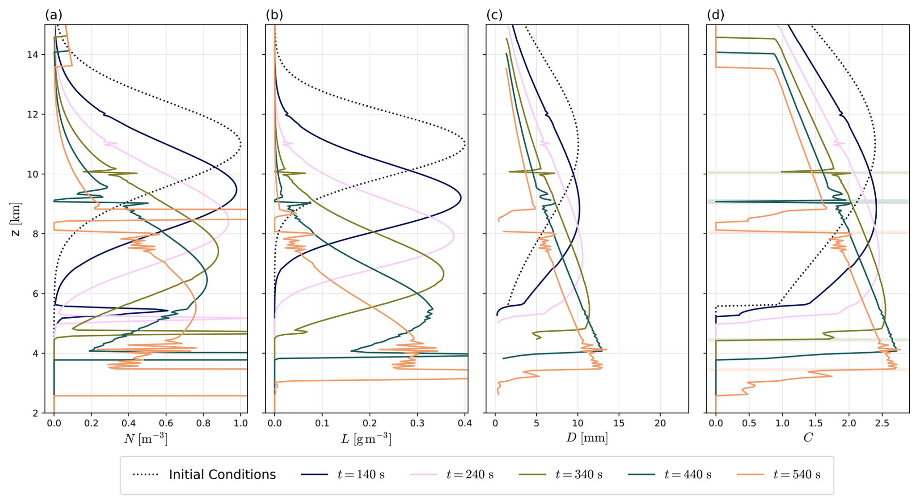
Figure B1 Hydrometeor profiles obtained using the explicit scheme (Sect. 2.3) in a single-column, pure sedimentation configuration, i.e., neglecting 𝒬_CCN and 𝒬^Δt from Eq. (27). We use the vertical resolution Δz=50 m with time step Δt=10 s, ρ≡ρ₀ is assumed everywhere, and ICON's hail hydrometeor parameters are used as listed in Table 2. We show the hydrometeor number density (a), mass density (b), and the diagnostic mean diameter (c), drawn where $L>q_{\text{crit}}={\mathrm{10}}^{-\mathrm{9}}$ kg m⁻³. In (d), the mass density's Courant number $C=\left|v_{\mathrm{1}}\right(N,L\left)\right|\mathrm{\Delta }t/\mathrm{\Delta }z$ is shown, and regions where the Lipschitz condition (ℬ<1) is violated are marked by the shading in the respective color. In the upper domain region, spurious oscillations slowly develop despite no Lipschitz condition violations, first visible at t=140 s, z=12 km, and subsequently at t=240 s, z=11 km. At t=340 s, z=10 km, ℬ>1 is reached for the first time, such that oscillations further grow and the originally single-peak profile is split in two (t=540 s). Oscillations in the lower domain region are initially induced by the operator 𝒟 from Eq. (27), since it sharply increases the number density.

Appendix C: Additional figures for case studies

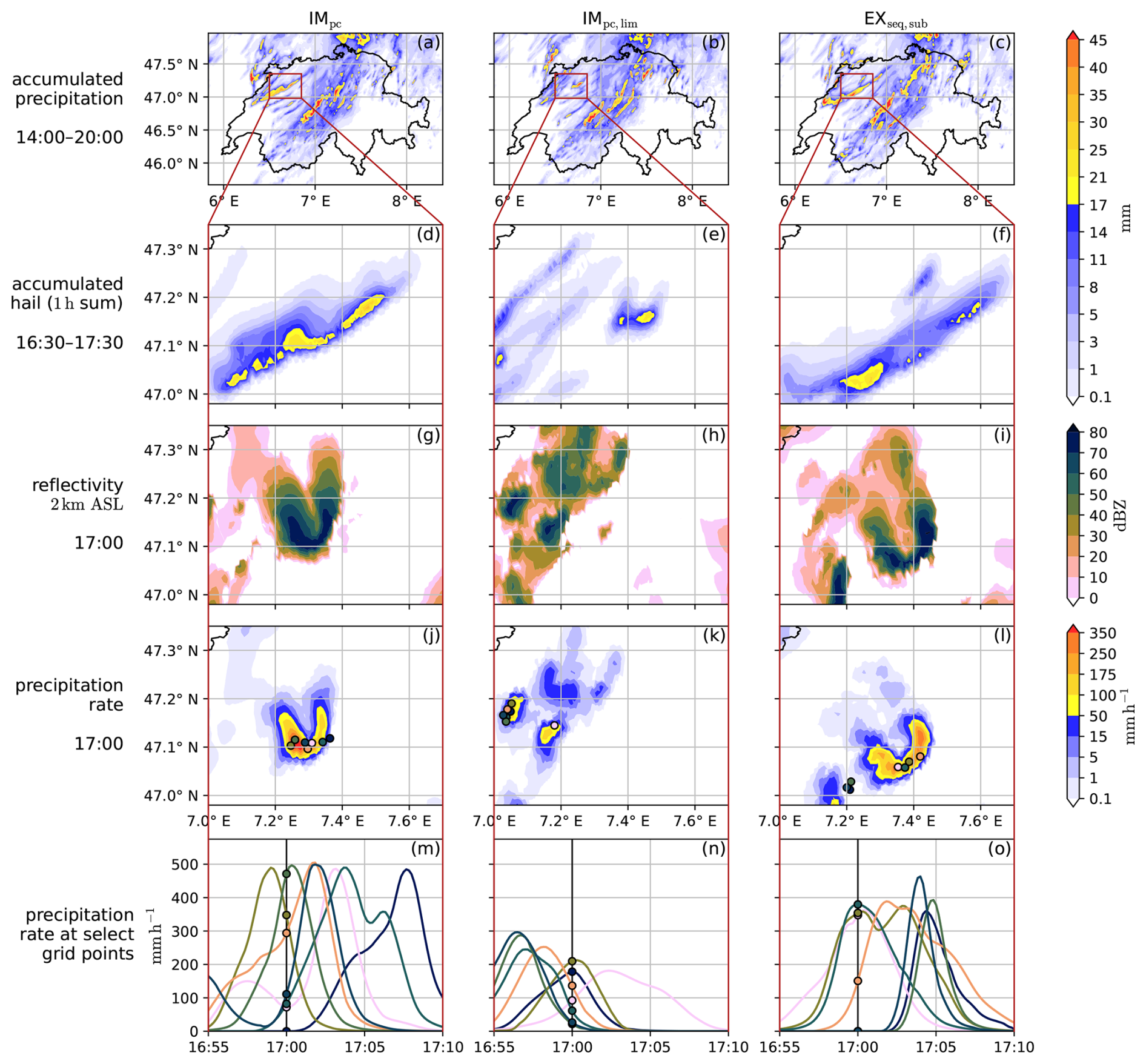
Figure C1 For the 20 July 2022 case and the IM_pc, IM_pc,lim, and EX_seq,sub configurations, the accumulated precipitation from 14:00–20:00 UTC over the entire simulation domain is shown in the first row (a–c). The following rows give a zoom–in view of a severe storm over the Jura mountains, specifically the 1 h accumulated hail (d–f), radar reflectivity at 2 km a.s.l. (g–i), and instantaneous precipitation rate at 17:00 UTC (j–l). The last row (m–o) displays the time evolution of precipitation rates for a few select grid points whose locations are marked in the row (j–l) above.

Figure C2 Time series of precipitation rate roughness, Eq. (29), for all six cases.

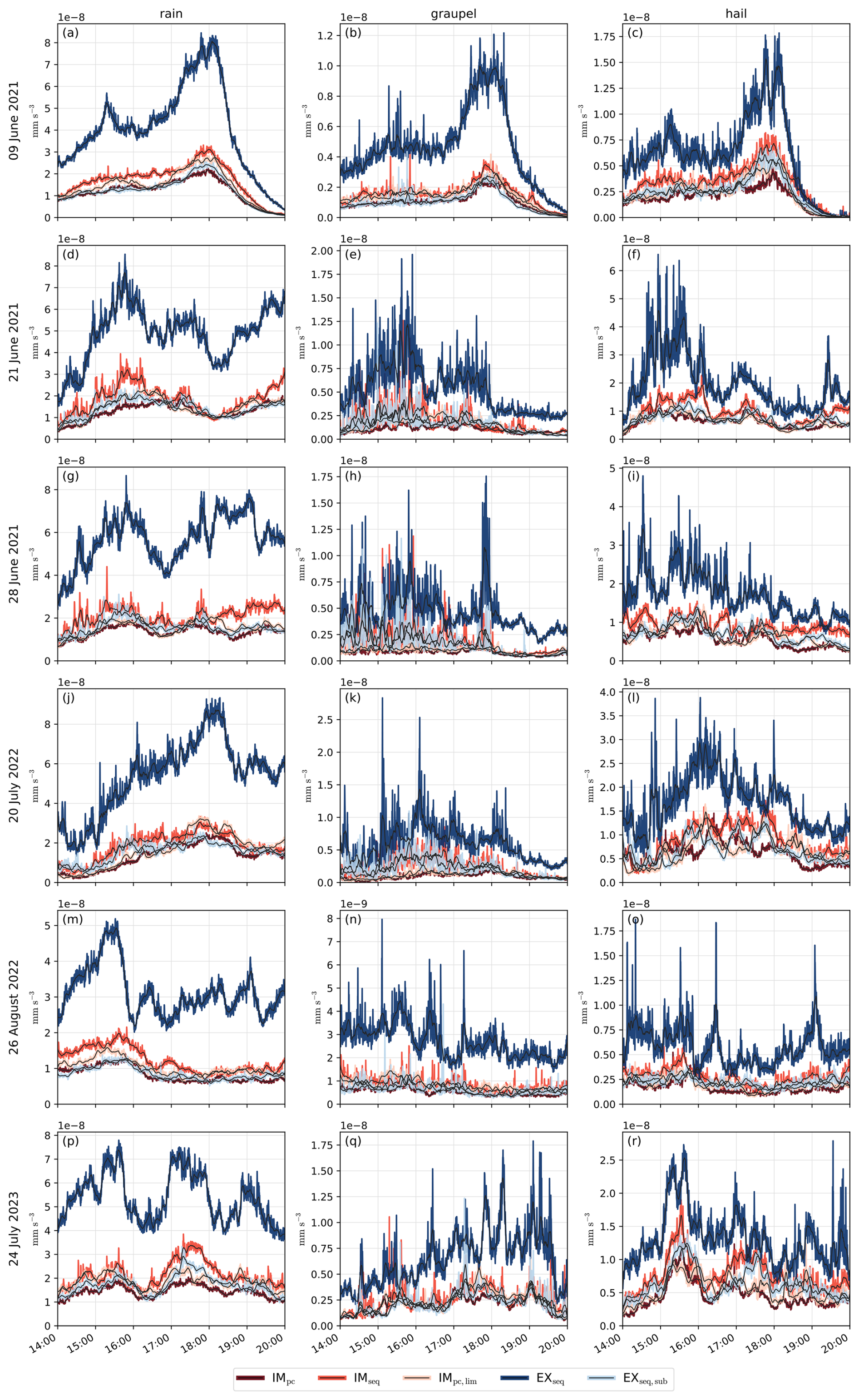
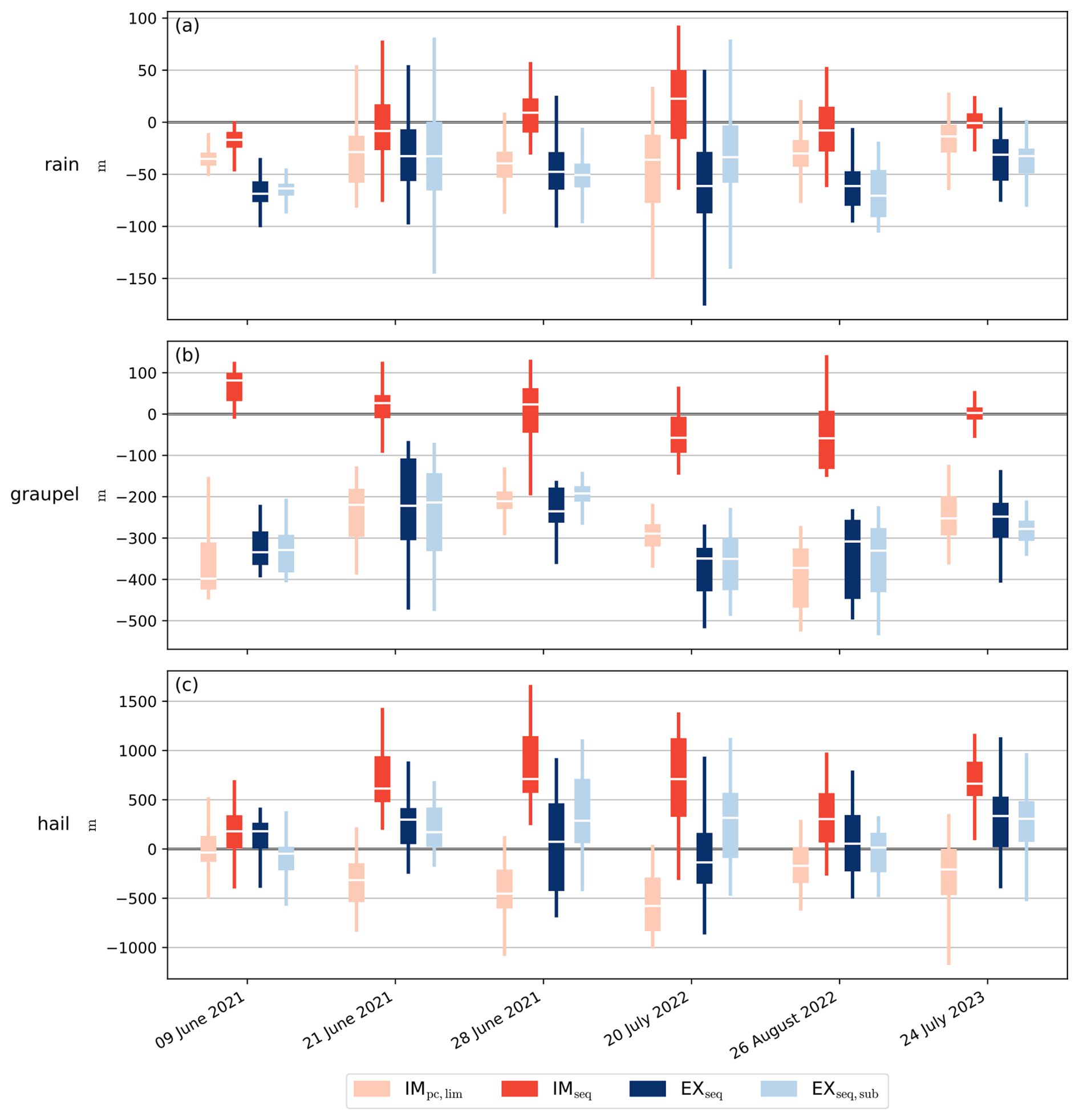
Figure C3 Difference of the mean upper q_crit threshold height (i.e., the spatial mean of the highest level's height with $L>{\mathrm{10}}^{-\mathrm{6}}$ kg m⁻³, over the columns where such threshold exists), to the default semi-implicit scheme IM_pc; for the time period 14:00–20:00 UTC with 10 min sampling interval. This is similar to Fig. 8, except for using the significantly larger threshold 10⁻⁶ kg m⁻³ instead of $q_{\text{crit}}={\mathrm{10}}^{-\mathrm{9}}$ kg m⁻³. For rain and graupel, the height difference trends are qualitatively similar to Fig. 8 but roughly half the size. For hail, the explicit configurations approximately match the IM_pc variant. In some cases, the less restrictive flux limiter IM_pc,lim slightly reduces the threshold's height, while the IM_seq configuration increases it.