A sea ice free Arctic: CMIP7 Assessment Fast Track abrupt-127k experimental protocol and motivation

Given that the Arctic could be ice-free in summer within the next ten to 20 years, accurately predicting low-ice states is of crucial importance. Paleo-evidence shows that the strong orbitally-induced high latitude insolation anomaly at 127 000 years ago (127 ky), of around +70 W m⁻² in the Arctic during spring-summer, led to warm conditions and an Arctic that was occasionally or often ice-free during summer. Building on two Coupled Model Intercomparison Projects (CMIPs): the Sea-Ice Model Intercomparison Project and the Paleoclimate Modelling Intercomparison Project, we propose an Assessment Fast Track experiment, abrupt-127k, focusing on this seasonally ice-free, or near ice-free, Arctic at 127 ky. The abrupt-127k experiment is initialised from a piControl simulation and abruptly imposes observed values for the insolation distribution and greenhouse gas forcing at 127 ky. It provides a new opportunity to evaluate models used to compute climate projections, both against paleo-evidence and each other, during a known low Arctic sea ice state. As CMIP models are not usually tuned to paleo observations, abrupt-127k represents a true “out-of-sample” test. The abrupt-127k experiment has four key scientific objectives, to: ascertain the simulated Arctic sea ice state, including the presence and characteristics of last-ice areas; evaluate the simulated climates using Arctic paleo-evidence; characterise the central Arctic surface energy budget; and analyse the ice budget including ice melt, growth, and transport. We show that a large Arctic ice response will manifest within the first 30 years of the simulation, thus a single 100-year long run is sufficient for these objectives. Modelling groups are requested to follow standard CMIP output protocol for analysis, including the use of standard “fixed-length” output. Given abrupt-127k is similar in setup to abrupt-2xCO2 and abrupt-4xCO2 CMIP7 experiments, combined analysis of these abrupt-experiments will facilitate understanding of the impacts of instantaneous radiative forcing in the Arctic.

1 Introduction

Predictions of first occurrence, extent, and characteristics of an ice-free Arctic rely on climate projections. These projections are usually derived using some combination of historical observations (Paik et al., 2023) and output from Coupled Model Intercomparison Project (CMIP) simulations under future emission scenarios (e.g. Meinshausen et al., 2011; Riahi et al., 2017). The CMIP models themselves are typically evaluated by comparing historical simulations with observations. Satellite observations commonly used include sea ice area (available since 1979) and sea ice volume (available since 2010). However, this approach to evaluating CMIP models has a major weakness when applied to Arctic sea ice: many CMIP-based future projections suggest an ice state that is outside the historical observational ranges used for model evaluation.

The earliest ice-free day could occur in the Arctic within the current decade (Heuzé and Jahn, 2024; Jahn et al., 2024). The earliest practically ice-free month, or seasonally ice-free state, is likely to occur by 2050 under all emission trajectories (Kim et al., 2023), where the term “practically ice-free” is defined as an Arctic sea ice area of less than 1 × 10⁶ km² (IPCC, 2021). Projected ice losses begin in the European Arctic, proceed to the Pacific Arctic, and end in the Central Arctic (Jahn et al., 2024). Given the Central Arctic region is expected to be the region that retains sea ice for the longest, it therefore holds particular relevance for projecting the timing of the first ice-free state (Paik et al., 2023). It would be helpful to be able to assess whether “last-ice-areas”, and whether growth and melt of sea ice under near ice-free conditions are consistently represented in CMIP models (Paik et al., 2023). Paleoclimate observations, and the simulation of past warm climates with little Arctic sea ice, can provide valuable information on the future (e.g. Bracegirdle et al., 2019), including through providing strong out-of-sample tests for CMIP, through the Paleoclimate Modelling Intercomparison Project (PMIP) (Braconnot et al., 2021; Kageyama et al., 2024).

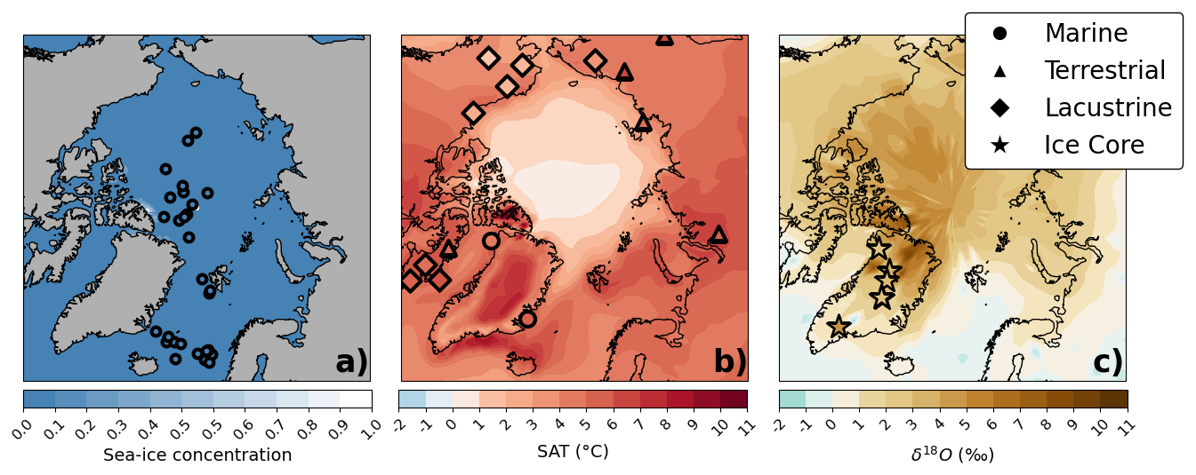
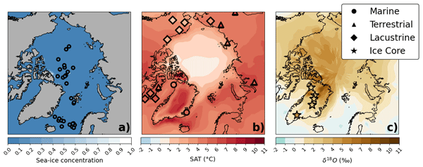
Figure 1 Three lines of evidence for a sea ice free Arctic at 127 ky. (a) Marine core evidence for the minimum sea ice concentration at 127 ky: occurrences of T. quinqueloba (Vermassen et al., 2023), with the climatological minimum-month (September) sea ice concentration from a lig127k simulation run with HadGEM3 (Guarino et al., 2020). (b) Simulated summer (an average of June to August) surface air temperature anomalies from the lig127k HadGEM3 simulation, overlaid with reconstructed summer temperature anomalies (Sime et al., 2023). (c) Ice core δ¹⁸O anomalies from seven Greenland ice core sites (stars) (Domingo et al., 2020), superimposed on simulated annual mean precipitation-weighted δ¹⁸O anomalies from a lig127k HadCM3 simulation with an ice-free summer Arctic Ocean (c.f. Malmierca-Vallet et al., 2018).

Reconstructions from marine cores, ice cores, and land-based Arctic cores indicate that the Arctic was warm and seasonally ice-free around 127 000 years ago, or 127 ky (Fig. 1; NEEM community members, 2013; Domingo et al., 2020; Kageyama et al., 2021; Vermassen et al., 2023; Sime et al., 2023). This was driven by the large summertime top-of-atmosphere (TOA) shortwave radiation anomaly in the Arctic of 60–80 W m⁻² (Fig. 3), which caused the loss of Arctic ice during summer (Guarino et al., 2020). Three independent lines of evidence support this. (1) The presence of the open-water T. quinqueloba species in Arctic marine sediment cores (Vermassen et al., 2023). (2) Summer surface air temperature anomalies from simulations and observations, indicate that model results match the observed warm 127 ky Arctic summers when the Arctic was seasonally ice-free (Guarino et al., 2020; Sime et al., 2023; Crow and Prange, 2025). (3) Greenland ice core 127 ky δ¹⁸O anomalies, which are only captured by seasonally ice-free simulations (Malmierca-Vallet et al., 2018; Domingo et al., 2020; Sime et al., 2025). Together, these independent lines of evidence strongly support the conclusion of an occasionally or often (seasonally) ice-free Arctic around 127 ky.

The presence of a warm Arctic at 127 ky, allows the CMIP community to investigate and evaluate models under low-ice conditions. CMIP priorities include: addressing current inter-model differences in Arctic sea ice thickness, ice volume, speed of the loss of ice, timing of the sea ice maximum, sea ice volume during minimum conditions, and plausibility of changes in sea ice and global mean surface temperature (Notz and SIMIP Community, 2020). Improved knowledge under greenhouse and ice-sheet conditions that are rather like those of the pre-industrial (Otto-Bliesner et al., 2017) will facilitate comparison of warm Arctic model projections, and can help ensure appropriate weighting of models, when model simulations are used in future projections (Paik et al., 2023; Selivanova et al., 2024). This is important because Arctic climate variability and the large range of model simulation results add to uncertainties in Arctic sea ice projections. The 127 ky conditions allow assessment of “last-ice-areas”, surface energy budgets, and whether growth and melt of sea ice in near ice-free conditions are different between CMIP models. This helps show whether CMIP7 models are improved compared to CMIP6/PMIP4, and so may help improve climate model skill in the Arctic.

The Sea Ice Model Intercomparison Project (SIMIP) has helped advance the analysis of modelled sea ice, including by moving the community away from an over-reliance on ice extent (Notz et al., 2016). Its focus on heat, momentum, and mass budgets has helped address key uncertainties in ice behavior. For example, Keen et al. (2021) used SIMIP recommended diagnostics and protocol in their multi-model analysis of the mass budget of Arctic sea ice. The focus on ice growth and loss processes helps diagnose reasons for the spread in Arctic sea ice extent and volume across CMIP6 models. Similarly, West and Blockley (2025) used SIMIP diagnostics to identify systematic biases in CMIP6 models, such as excessive summer melt and winter growth. Whilst CMIP models agree on the dominant influence of greenhouse gas forcing on current Arctic ice declines, these systematic biases, related to the representation of key ice melt and growth processes, may lead to underestimation of future ice decline (Notz and SIMIP Community, 2020; Kim et al., 2023). The physics of sea ice sub-models and polar amplification in the coupled climate will largely determine how CMIP models respond to the large abrupt-127k summertime TOA shortwave Arctic anomaly (Guarino et al., 2020; Diamond et al., 2021; Kageyama et al., 2021; Diamond et al., 2023; Sime et al., 2023). The use of SIMIP diagnostics for analysis of the modelled abrupt-127k sea ice changes will provide invaluable information on CMIP7 sea ice sub-model processes and parameterizations that control sea ice during warm Arctic conditions.

For the upcoming CMIP7, there will be a two-tiered timeline for producing simulations (Dunne et al., 2025). The CMIP7 Assessment Fast Track runs on a tighter schedule than the wider CMIP7 community effort and contains those simulations of particular importance for the next IPCC Assessment Report. The abrupt-127k experiment proposed here is a core contribution of PMIP to the CMIP7, and this abrupt-127k protocol paper is one of a suite associated with the CMIP7 Assessment Fast Track and the corresponding data request. The abrupt-127k protocol draws heavily on the previous CMIP6/PMIP4 lig127k protocol (Otto-Bliesner et al., 2017). We note that the lig127k experiment tests how well climate models simulate this past warm period by benchmarking their responses to known forcings against palaeoclimate evidence from across the globe, whilst the shorter abrupt-127k experiment focusses solely on the Arctic. The close relationship between the lig127k and abrupt-127k helps ensure traceability of the impact of model development cycles on the simulations. In addition to providing practical instructions for the set-up of the abrupt-127k experiment, this paper is intended to help ensure effective single- and multi-model analysis of simulations. It provides clear instructions on how model groups should analyse the sea ice response in their Assessment Fast Track abrupt-127k simulations.

There are four primary scientific objectives of abrupt-127k, which can each be potentially tackled individually by each modelling group. These are to:

• 1.

  Ascertain the simulated abrupt-127k Arctic sea ice state, including the extent of last-ice-areas and other regional low-ice changes.

• 2.

  Assess the simulated state against 127k reconstructions of summer temperatures and sea ice (see Fig. 1a and b).

• 3.

  Characterise the central Arctic abrupt-127k surface energy budget (e.g. Guarino et al., 2020; Diamond et al., 2021; Kageyama et al., 2021; Diamond et al., 2023).

• 4.

  Analyse abrupt-127k ice budgets with a focus on the common melt and growth terms (Notz et al., 2016; Keen et al., 2021; West and Blockley, 2025).

Three further objectives require analysis of Assessment Fast Track output beyond the abrupt-127k and the piControl experiments. These are to:

• 5.

  Establish how abrupt-127k results relate to other Fast Track instantaneous model adjustment experiments, particularly abrupt-2xCO2 (Kageyama et al., 2021; Otto-Bliesner et al., 2021).

• 6.

  Map results from these two “abrupt” simulations to both polar amplification and equilibrium climate sensitivities of each particular model (Guarino et al., 2020; Kageyama et al., 2024).

• 7.

  Use results of objectives 1–5 to improve weighting of individual model outputs when making projections of future Arctic sea ice-losses (e.g. Notz and SIMIP Community, 2020; Paik et al., 2023; Jahn et al., 2024; Selivanova et al., 2024).

In this manuscript we focus largely on the first four of these objectives, which can be achieved by each individual modelling group using their own model output. After providing the experiment design for abrupt-127k, i.e. the instructions to set-up and run the experiment, the manuscript provides an example to illustrate how we recommend that CMIP7 modelling groups analyse abrupt-127k output towards achieving these first four objectives. The latter (5–7) objectives may be best achieved in subsequent CMIP7 community-led multi-model analyses.

2 Experimental design for the abrupt-127k and data request

This subsection lays out the information required to set up and run the abrupt-127k experiment. We start by providing additional information on the history of abrupt-127k, and an overview of previous similar CMIP6-PMIP4 experiment results.

2.1 Background and previous CMIP6-PMIP4 simulations

The Paleoclimate Modelling Intercomparison Project has served to coordinate paleoclimate experiments and data–model comparisons for several decades, including the paleoclimate contribution to CMIP6 (Eyring et al., 2016; Kageyama et al., 2018; Braconnot et al., 2021). A Last Interglacial experiment, lig127k, was defined for CMIP6/PMIP4 (Otto-Bliesner et al., 2017), and has been run by 16 CMIP6 models (Otto-Bliesner et al., 2021). The main difference between the piControl and lig127k experiments is the large summertime TOA shortwave radiation anomaly (Otto-Bliesner et al., 2017).

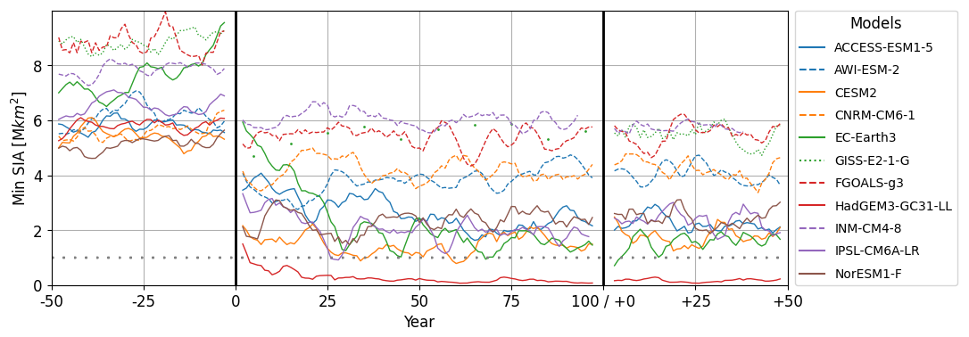
Figure 2 Multi-model evolution of Arctic sea ice area (SIA) minima. 5-year running average of minimum monthly SIA per model for the piControl (left panel), first 100 years of lig127k spin-up (centre panel), and fully spun up lig127k (right panel). Solid lines are used for model simulations with at least one practically ice-free summer during the spin up. Dotted lines indicate the model simulation does not drop below the practically ice-free threshold, of 1 × 10⁶ km² in SIA (shown with horizontal gray dotted line).

All the CMIP6 models that participated in the lig127k simulation have been shown to simulate substantial reduction in summer sea ice compared to the piControl (Otto-Bliesner et al., 2021; Kageyama et al., 2021), indeed at least three models show summer ice-free conditions during their spun-up lig127k simulation (Diamond et al., 2021; Sime et al., 2023). The duration of these experiments is most commonly around 350 years. It is useful to establish if significant Arctic sea ice changes occur over shorter duration simulations. We thus compile the first 100 years of output from these CMIP6 lig127k simulations – this is typically considered model “spin-up”. There are 16 CMIP6 models that have run lig127k, but not every model group kept their first 100 years of spin-up data. We have nonetheless obtained 11 sets of spin-up lig127k CMIP6 simulation output (Fig. 2). These first 100 years of the CMIP6 lig127k simulations show that, for the majority of the models, an immediate sea ice response to the insolation forcing occurs within the first couple of decades. Indeed all of the models suggest that a new Arctic sea ice state will be reached within the 100 years of the start (year 0, Fig. 2).

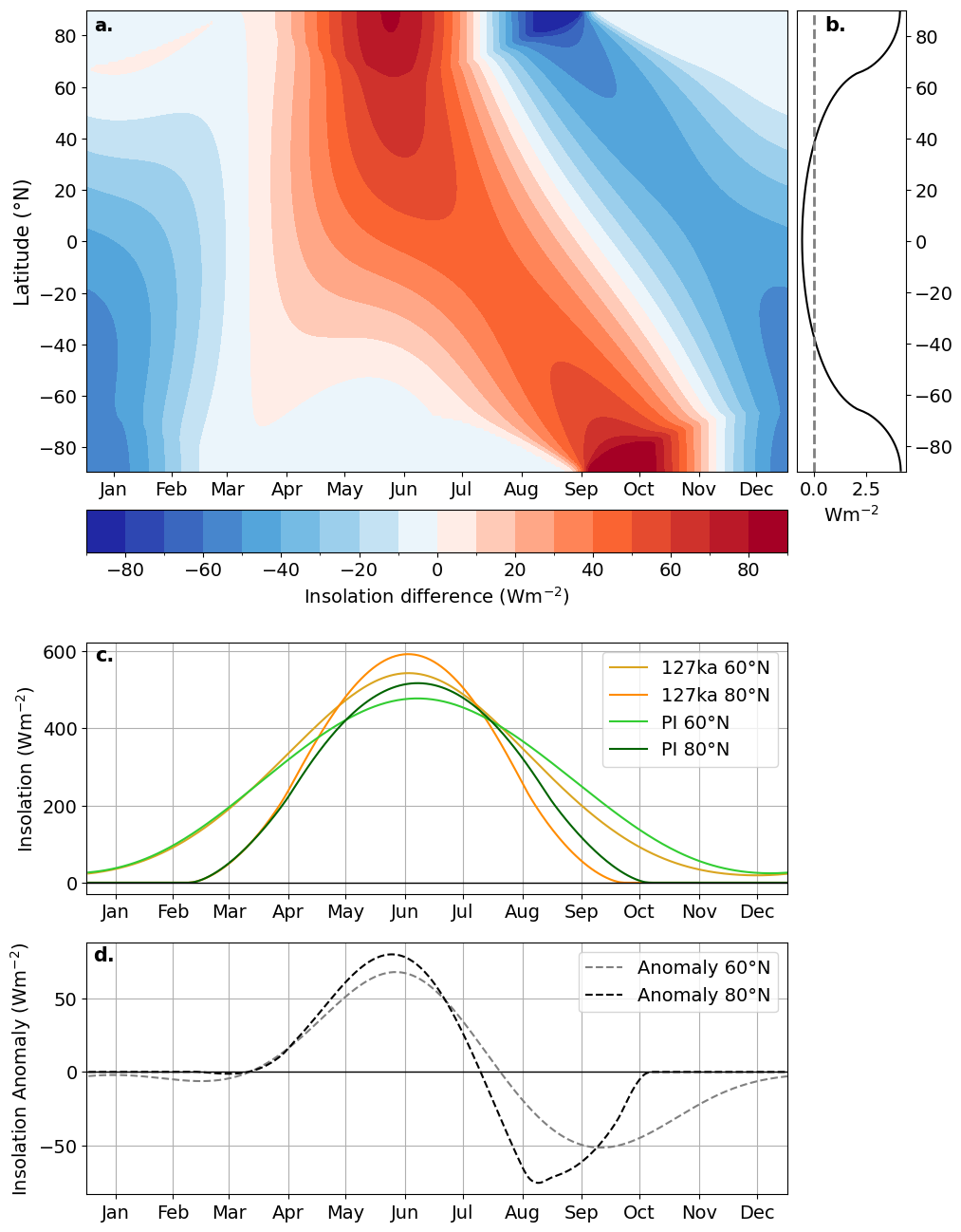
Figure 3 Characteristics of top-of-the-atmosphere (TOA) insolation anomaly between 127 ky and present. (a) Hovmöller plot of latitudinal insolation anomalies across the year. (b) Annual average of data shown in (a). (c) Seasonal cycle of TOA insolation for two latitudes in the Arctic for both 127 ky and pre-industrial. (d) Anomalies of data in (c) as 127 ky – pre-industrial.

Table 1 Experimental set-up – forcings and boundary conditions for the essential (Tier 1) and the (CMIP6) piControl abrupt-127k simulation. Note that greenhouse gas concentrations and total solar irradiation for the CMIP7 piControl (1850) are not yet published. Once available, CMIP7 values should take precedence.

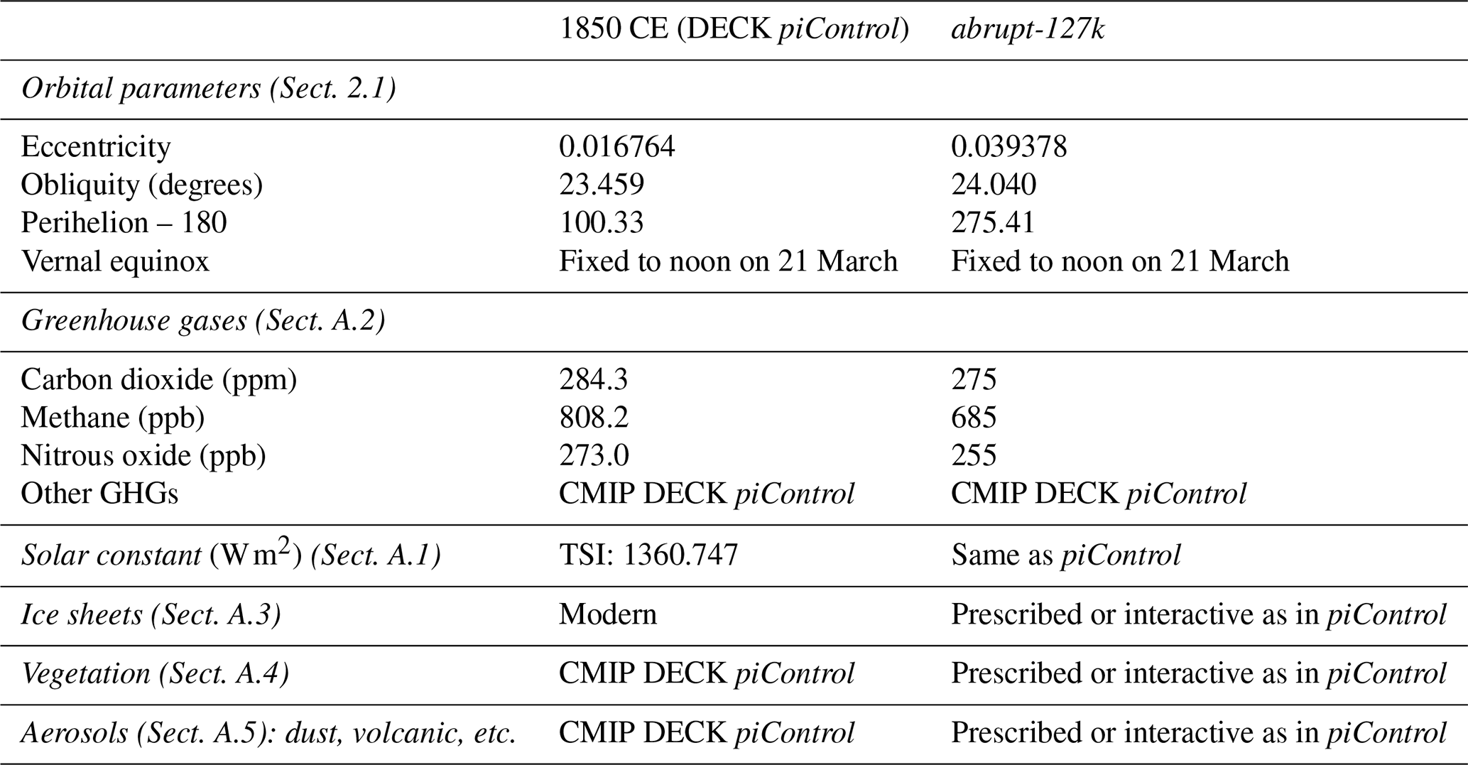
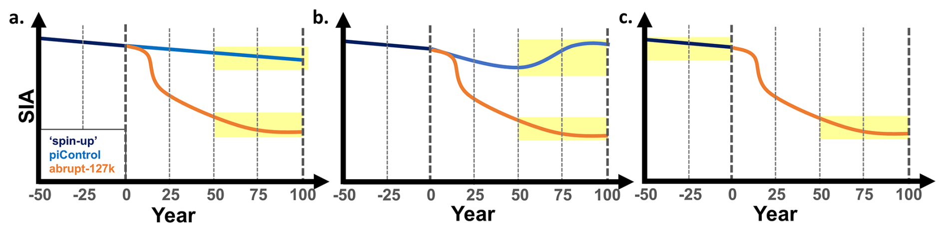
Figure 4 Recommendations for choice of years of piControl which should be used for comparison to abrupt-127k. Recommended procedure is to run both experiments on from the same branch point (same initial condition at year 0). This means that any (a) residual simulation drift and/or (b) low frequency variations can occur in both experiments. If piControl is not run on from the branch point, (c) illustrates that in this case, we recommend differencing from closest pre-branch portion of the piControl (here denoted the “spin-up” simulation and shown in navy).

2.2 Experiment protocol and data request

The abrupt-127k experiment is a single-member, relatively short simulation that requires minimal set-up and modest computational resources. It should be branched from a suitably spun-up CMIP7 DECK (Diagnostic, Evaluation and Characterization of Klima) piControl simulation (Fig. 4). Changes to insolation and greenhouse gas concentrations should follow the specification in Table 1 (see also Fig. 3). Configurations for vegetation, topography, aerosols, and land-sea mask should remain the same as for the piControl. Given the ice decline is rapid (Fig. 2), with an ice-free state reached within 10 to 50 years for some models (Fig. 2), a 100-year simulation length is the minimum required. Modelling groups are advised to perform a basic check to ensure their first year TOA output matches Fig. 3.

Because abrupt-127k (and/or abrupt-2xCO2) is branched from, and directly comparable with piControl, it is rather simple to set-up. The set-up details are based on its predecessor CMIP6 lig127k protocol (Table 1; Otto-Bliesner et al., 2017). However once CMIP7 piControl set-up details are available, this experiment should take precedence over the CMIP6 piControl. Whilst the Table 1 overview should be sufficient for set-up, for the interested reader a fuller explanation of the protocol and its rationale is provided by Otto-Bliesner et al. (2017). Or see Appendix A for further details.

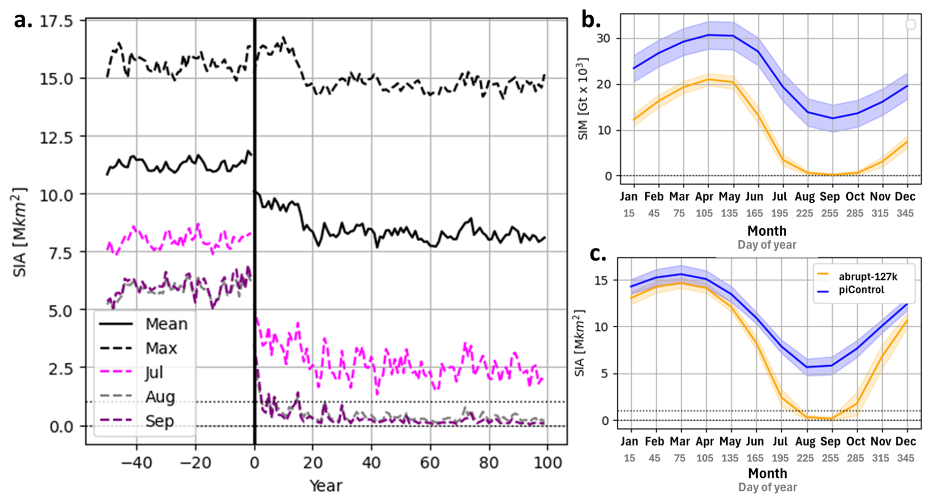
Figure 5 Timeseries and seasonal cycle of Arctic sea ice area (SIA) and sea ice mass (SIM) for the example HadGEM3 abrupt-127k simulation. (a) Timeseries of sea ice area (SIA) from years 0 to 100 of abrupt-127k. piControl (shown as years “−50–0”) and abrupt-127k (years 0–100). SIA for (pink) July, (grey) August, (purple) September each year, with annual mean SIA as a solid black line, and monthly maximum SIA each year as a dashed black line. After Diamond et al. (2021). Mean monthly value (solid line and shaded area showing twice the standard deviation), for (b) SIA, and (c) sea ice mass. We use years 51–100 of abrupt-127k (orange) and the equivalent years of piControl (blue); HadGEM3 uses a 360 d calendar, so along the x axis we show both the month and the central “day of the year” for this month in the 360 d calendar. See Appendix C for SIA and SIM definitions.

Given we recommend calculating differences between each abrupt-127k simulation with its comparable piControl simulation, the preferred spin-up and procedure for each model is to run both abrupt-127k simulation and piControl simulation from a shared start file, and analyse abrupt-127k relative to the corresponding 100 years of piControl. This spin-up and analysis procedure minimises the impact of any drift or internal variability in the piControl simulation (Fig. 4a and b). If the equivalent 100 years of the piControl simulation is unavailable, then the closest 50-year period should be used instead (Fig. 4c). Modelling groups are advised to plot a timeseries of annual Arctic SIA (Sea Ice Area) from both piControl and abrupt-127k, like Fig. 5, to assess potential model drift before undertaking any analysis.

Table 2 Essential monthly atmospheric model variables. CMIP7 Table identifier: Amon (monthly atmosphere output). All variables are included in standard CMIP7 model output.

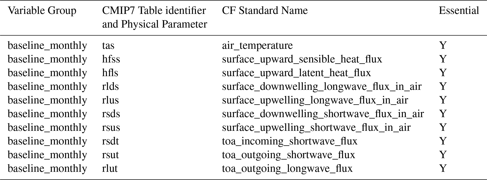
Table 3 Essential (and optional) sea ice and ocean model variables. All required variables are from monthly output. All variables should be included in abrupt-127k model output, as part of requested variable groups “baseline_monthly”, “baseline_daily”, “seaice_state_monthly_basic”, “seaice_budget_mass_monthly”, and “seaice_state_monthly_advanced”. Variables indicated with an asterisk (^∗) are calculated over the ice-covered region of the grid cell only; otherwise, variables are calculated over the whole grid-cell area.

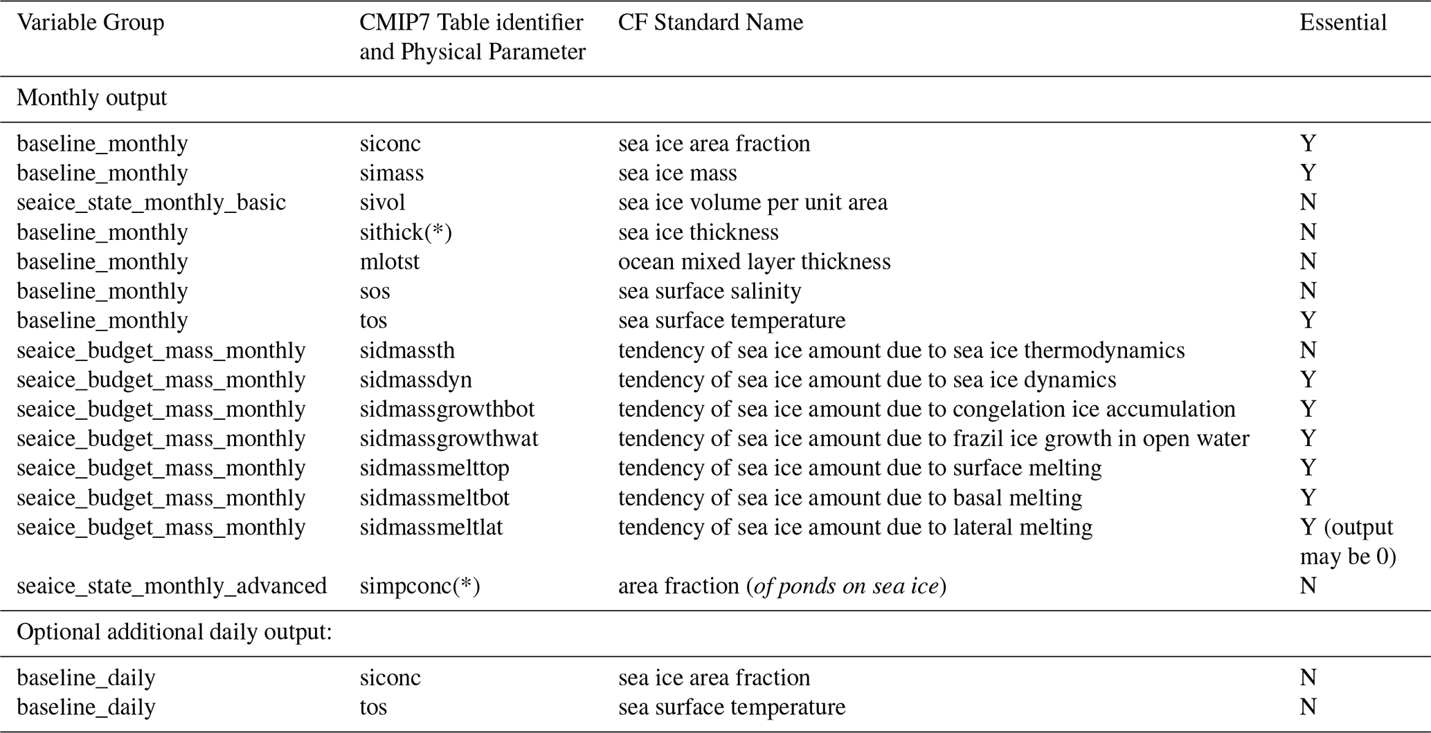
Required monthly variables for the recommended subsequent analyses are given in Tables 2 (atmospheric variables) and 3 (sea ice and ocean variables). These are primarily drawn from Fox-Kemper et al. (2025), who present the full CMIP7 ocean and sea ice data request; modelling groups who are interested in having their abrupt-127k simulation embedded in the wider PMIP framework are invited to consider this full PMIP data request. See also Juckes et al. (2025) for further information on baseline CMIP climate variables. Ice-related quantities shown (ice concentration, mass, pond-related quantities, and growth- and melt-related quantities for the sea ice budgets) are calculated over all Northern Hemisphere grid-cells. The atmospheric and oceanic quantities (surface air temperature and energy budgets) should be calculated over the central Arctic: 70–90° N, with no land mask applied, as in Kageyama et al. (2021, Figs. 8 and 9). Groups may find it useful to regrid variables using the CDO library, or equivalent, to a regular 1° latitude-longitude grid before analysis.

Following the standard CMIP7 approach, the experiment described in Table 1 is considered to be a Tier 1 experiment and is the only required experiment for this protocol. However two additional, non obligatory, Tier 2 experiments are detailed in Appendix B. If run, these two additional simulations will enable interested groups to: (i) isolate the impacts of vegetation-feedback on Arctic climate, and (ii) explore longer term, global-scale response under 127k boundary conditions, i.e. perform the PMIP lig127k experiment which would allow studies of other features of the Last Interglacial climate.

2.3 Monthly and seasonal averaging: “fixed-length” versus “fixed-angle”

There are generally two ways to define months or seasons (or any other portion of the year): (1) “fixed-length” whereby months or seasons are defined by a fixed number of days, and (2) “fixed-angle” where months or seasons are instead defined by a fixed angular segment of the Earth's orbit e.g. 30° or $\mathrm{1}/\mathrm{12}$ of a full revolution of Earth's orbit per month (Bartlein and Shafer, 2019). This is true for both present and past climate conditions. Climate models calculate TOA quantities for each day and across the years, and correctly aggregate monthly and seasonal output over a fixed number of days. This matches the fixed-length definition of time-averaging.

By convention, the vernal equinox is fixed as occurring on 21 March (Fig. 3a). Because the Earth moves fastest near perihelion (when Earth is closest to the sun) and slowest near aphelion (when Earth is farthest from the sun), the use of a fixed-angle calender would cause problems in the calculation of energy budgets (e.g. Otto-Bliesner et al., 2017; Bartlein and Shafer, 2019). This is because use of a fixed-angle calendar results in months and seasons of unequal day-lengths. Given that the abrupt-127k experiment is focused on the correct calculation of ice energy and mass budgets, abrupt-127k requires the use of standard-CMIP fixed-length output for the majority of analyses; adjusting to use a fixed-angle calendar would lead to incorrect lengths of melt, ice-free, or ice growth seasons, and associated aggregated energy-budget terms. For this reason we explicitly request that groups do not re-aggregate variables onto fixed-angle months using PaleoCalAdjust (Bartlein and Shafer, 2019), or its equivalent, for the analyses proposed here.

Advancements and delays relative to the solstices (of 6 and 7 d) and autumnal equinox (of 13 d) will affect piControl against abrupt-127k comparisons using normal fixed-length output – indeed, this is the problem that fixed-angle calendars address. By definition, the vernal equinox is however always identical for both experiments. Solstice and equinox, more generally angular, shifts will affect the calendar dates associated with ice melt or growth onset at 127k. Groups are encouraged to plot variables as a function of day-of-year or fraction-of-year, rather than by calendar date, to help minimise these issues.

Any interpolation issues aside, the lengths of the melt or growth seasons – and budgets – associated with these processes will be correct when using normal fixed-length (daily, monthly, or seasonal) data. However modelling groups may wish to provide and use daily sea ice concentration data (Table 3), as that reduces any interpolation errors in the calculation of ice-free days and associated budget terms. Daily data can also be used in the investigation of calendar-related artifacts studies, for groups interested in angular-shift effects.

3 Arctic sea ice analyses

This section details recommended analyses to achieve science objectives 1–4 for abrupt-127k. We demonstrate the approach using output from an example CMIP6 model: HadGEM3-GC3.1-LL (hereafter HadGEM3), which uses a 360 d calendar made up of twelve 30 d months. The scientific objectives of these analyses, focused on the abrupt-127k Arctic, are primarily to: (1) characterise the sea ice state; (2) evaluate against 127 ky observational evidence; (3) examine the surface energy budgets; and (4) quantify the sea ice budget in terms of melt, growth and dynamics processes.

3.1 Overview of the analyse objectives and their intended aims

Here we divide these into main objectives e.g. O1.1, and further objectives e.g. FO1.4.

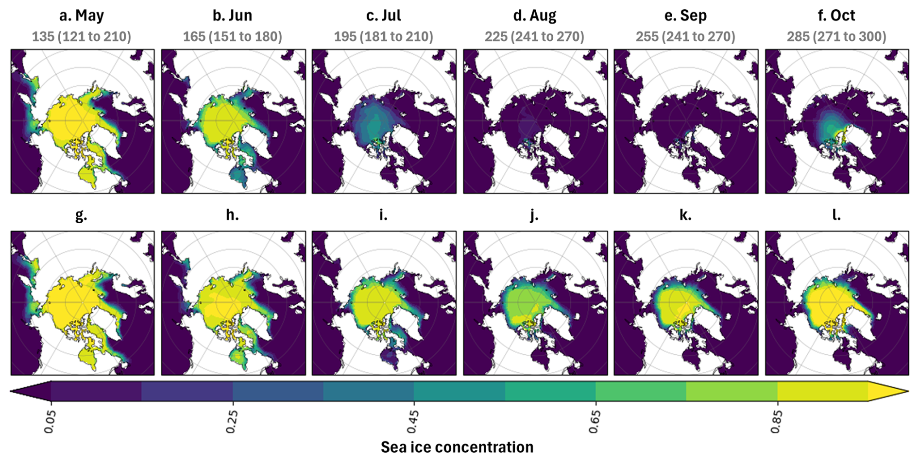
Figure 6 Maps of mean monthly sea ice concentration over years 51–100 of (a–f) abrupt-127k and (g-l) piControl simulations. Each month from May to October is shown. August and September are ice-free for abrupt-127k, but not for the piControl. HadGEM3 uses a 360 d calendar, so we show both the month, and the central “day of the year” (and range in brackets) for this month in the 360 d calendar.

3.1.1 Characterization of the abrupt-127k Arctic sea ice state

The first set of scientific objectives is to ascertain the abrupt-127k Arctic ice state, including examining the presence or absence of last-ice-areas and other expected regional low-ice changes, in the simulation. As in CMIP6, the Arctic sea ice response to abrupt-127k will likely differ between CMIP7 models (Kageyama et al., 2021; Sime et al., 2023), so it is important to characterise model-specific behavior. Key analyses include the rate of summer ice decline, determining whether the Arctic becomes seasonally ice-free, when this occurs, and whether a stable Arctic ice state is reached within the first few decades. Recommended analyses, and related objectives, are:

• O1.1 Confirm that the abrupt-127k Arctic sea ice reaches a new stable state within the first 50 simulation years (Fig. 5a).

• O1.2 Determine whether the abrupt-127k Arctic becomes seasonally ice-free, and if so, when this occurs (Fig. 5a).

• O1.3 Compare the climatological total ice area and mass between abrupt-127k and piControl (Fig. 5b and c).

• FO1.4 Investigate where in the Arctic ice remains through the summer, or where it is last lost and first regrown, as applicable (Fig. 6).

3.1.2 Assessment of Arctic abrupt-127k against 127k observations of summer temperature

The second scientific objective is to assess the simulated state against 127k observations of summer temperature and sea ice (see Fig. 1a and b):

• O2.1 Compare simulated abrupt-127k Arctic sea ice with summer surface air temperature observations (Fig. 1b; Guarino et al., 2020; Sime et al., 2023).

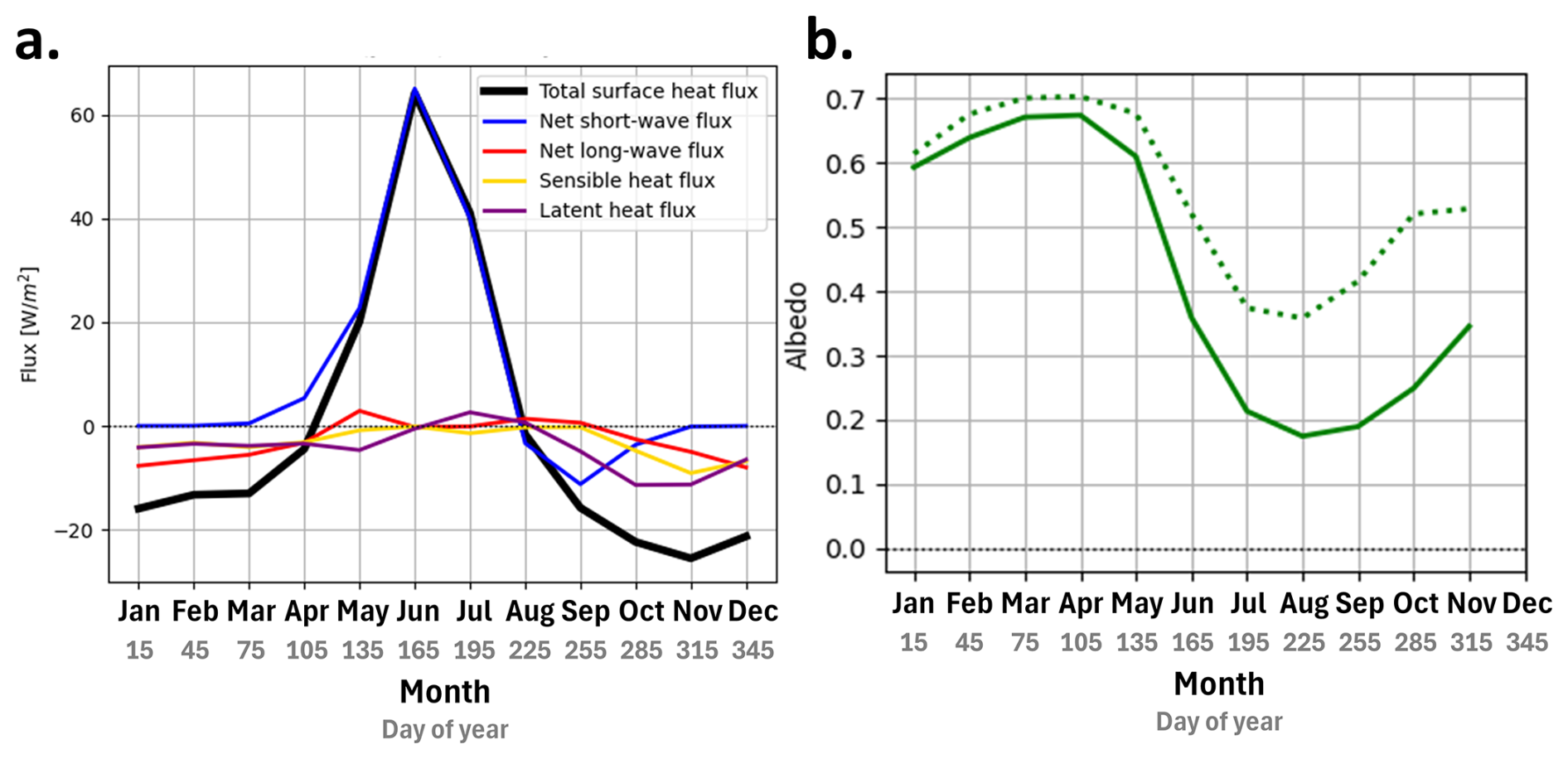
Figure 7 Arctic surface energy budget. (a) Monthly abrupt-127k – piControl anomaly of the surface energy budget, by components: net change in short-wave radiation, long-wave radiation, sensible and latent heat flux, and total heat flux (all measured positive downwards), following also Guarino et al. (2020) (Fig 3b); Diamond et al. (2021) (Fig. 5). (b) Mean Arctic albedo for abrupt-127k (solid line) and piControl (dotted line). All variables calculated as long-term mean over years 51–100 of abrupt-127k and piControl runs, over the central Arctic: 70–90° N, with no land mask applied. HadGEM3 uses a 360 d calendar, so along the x axis we show both the month and the central “day of the year” for this month in the 360 d calendar. See also Appendix C for further details on calculations.

3.1.3 Characterisation of the central Arctic abrupt-127k surface energy budget

The third scientific objective is to characterise the central Arctic abrupt-127k surface energy budget. Given the large changes in TOA forcing, recommended aims are to investigate the surface energy balance in terms of increased short-wave insolation, amplified by surface albedo feedback, resulting in Arctic warming and ice melt. Here, we focus on the Central Arctic region, defined as from 70 to 90° N (as in Diamond et al., 2021). Recommended analyses, and related objectives, are:

• O3.1 Assess the climatological changes in surface energy budget between abrupt-127k and piControl, in terms of change to surface energy components: short-wave and long-wave radiation, and latent and sensible surface heat fluxes (Fig. 7a).

• O3.2 Compare surface albedo change between abrupt-127k and piControl (Fig. 7b).

• FO3.3 Compare total downwards and net downwards short-wave radiation fluxes at the surface (Fig. A5a and b).

• FO3.4 Compare surface air temperature between abrupt-127k and piControl (Fig. A5c and d).

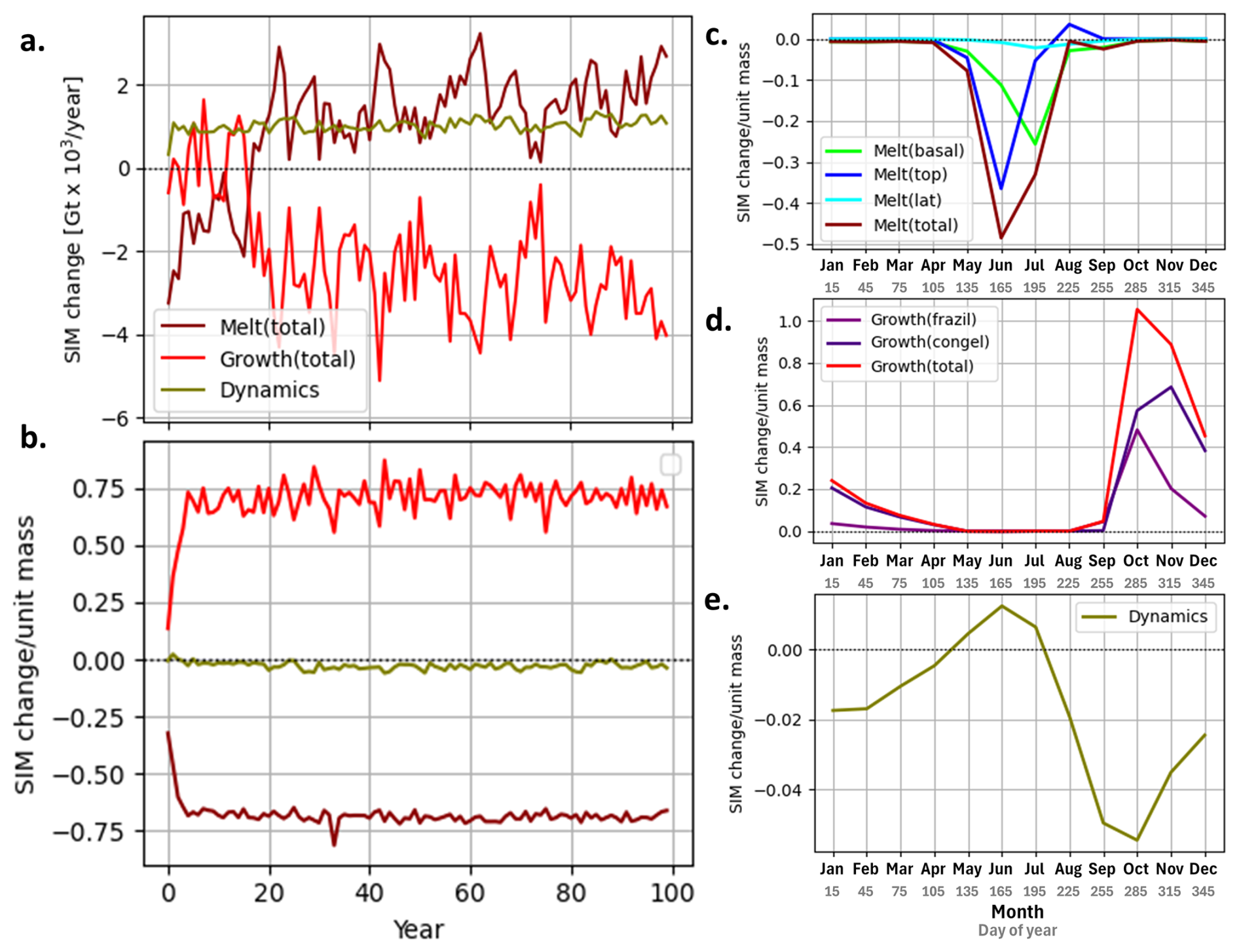
Figure 8 Melt and growth of Arctic sea ice for abrupt-127k. After Keen et al. (2021), we use a positive sign for ice increase and negative sign for ice decrease. Therefore, positive values indicate changes that increase SIM in the abrupt-127k compared to the piControl simulation (including increased ice growth and reduced ice melt), and negative values indicate changes that reduce SIM (decreased growth and increased melt). (a) Annual timeseries over all 100 years of abrupt-127k, with the mean over years 0–20 of the piControl simulation subtracted, for total growth (red) total melt (brown) and mass change due to dynamics (khaki). (b) Like (a), but with both abrupt-127k and piControl variables normalised by dividing by the SIM for each year, for each simulation. (c–e) Long-term means over years 51–100 of both the abrupt-127k and piControl simulations. These show climatologies of the abrupt-127k monthly mean (normalised by the mean monthly abrupt-127k SIM), with piControl monthly mean (normalised by the mean monthly piControl SIM) subtracted. We show both the month and the central “day of the year” for each month of HadGEM3's 360 d calendar. (c) Shows total melt (brown), estimated as the sum of top melt (blue), basal melt (green) and lateral melt (aqua), (d) shows approximate total growth (red), estimated as the sum of frazil growth (purple) and congelation growth (navy), and (e) shows change due to ice dynamics (khaki). See Appendix C4 for further details.

3.1.4 Characterization of the abrupt-127k sea ice budget

The fourth scientific objective is to quantify the ice processes. Ice changes due to thermodynamic (melt and growth), and dynamic processes on monthly and annual timescales. Specific analyses and objectives are to:

• O4.1 Investigate the total ice change with time (Fig. 8a).

• O4.2 Investigate the ice change per unit mass with time (Fig. 8b).

• O4.3 Compare the climatological differences in ice change per unit mass between abrupt-127k and piControl (Fig. 8c–e).

• FO4.4 As for O4.1-4.3, but using additional available diagnostics such as basal and top melt, and congelation and frazil growth (Figs. 8cde, A1, and A4).

• FO4.5 If a prognostic melt-pond scheme is available, compare melt pond formation and evolution between abrupt-127k and piControl (Figs. A2 and A3; Flocco et al., 2010; Hunke et al., 2013).

• FO4.6 Assessment of the clear-sky and total-sky (cloud) radiative effects is also encouraged (Tan and Storelvmo, 2019).

3.2 Handling of example model output

All quantities are calculated using outputs from HadGEM3, using the first 100 years of the spin-up period run under the lig127k protocol (Guarino et al., 2020). Time evolution figures use the full 100 years, climatological quantities use years 51–100. Hereafter this will be referred to as the HadGEM3 “abrupt-127k” simulation. For all figures, the abrupt-127k simulation is compared to the piControl simulation. Here, the abrupt-127k and piControl simulations were initialised from the same timepoint of the same simulation, so years 51–100 of both of these runs are used for the comparison (see Fig. 4). Required variables for subsequent analysis are listed in Tables 2 and 3. All variables are regridded using the CDO (Schulzweida, 2023) library to a regular 1° latitude-longitude grid before analysis, and are calculated using monthly mean data unless indicated otherwise. Ice-related quantities shown (ice concentration, mass, pond-related quantities, and growth- and melt-related quantities for the ice budgets) are calculated over Northern Hemisphere grid-cells. In line with SIMIP, we recommend using mass-related rather than volume-related quantities (Notz et al., 2016; Keen et al., 2021). Here, we show mass-related quantities, calculated by multiplying volume-related quantities by ice density (917 kg m⁻³). Appendix C provides additional methods detail that may be useful for groups undertaking recommended analyses.

3.3 Example results

This section shows the example results from HadGEM3 abrupt-127k simulation, which, under the lig127k protocol, simulated an ice-free Arctic (Guarino et al., 2020).

3.3.1 Characterization of the abrupt-127k Arctic sea ice state (O1)

We first quantify the time-evolution of SIA. Summer SIA is significantly reduced within the first 20 years of abrupt-127k for HadGEM3 (Fig. 5a; and Diamond et al., 2021). After year 10, the Arctic is seasonally ice-free in August and September every year. Furthermore, the annual and winter maximum also rapidly decrease: by year 20, SIA has approximately reached a new equilibrium state. This justifies the use of the climatologies shown hereafter (that use data from years 51–100 of HadGEM3 abrupt-127k).

Abrupt-127k shows a strong seasonal cycle in SIA and SIM (Sea Ice Area and Sea Ice Mass; Fig. 5b and c). Compared to piControl, abrupt-127k SIA is slightly reduced in the winter months and at least 2 M km² lower from June through November. The difference in SIM is less seasonal: SIM is consistently reduced year-round by 10–15 × 10³ Gt. Comparisons of the piControl and abrupt-127k SIC distributions through the summer (Fig. 6) show that the two simulations are generally consistent in May, but differences appear at the ice edge from June and expand across the whole Arctic by July. In abrupt-127k, the last remaining ice in July is over the central Arctic. By October, new ice begins to form near the north coast of Greenland, indicating a spatial shift in ice growth relative to piControl.

3.3.2 Assessment of Arctic abrupt-127k against 127k observations of summer temperature (O2)

In Fig. 1, the HadGEM3 simulation is assessed by visual comparison against three kinds of existing evidence. It is not anticipated that all groups will have the capability to diagnose changes in water isotopes (Fig. 1c), and work is ongoing to further refine the summer sea ice proxy compilation of Vermassen et al. (2023) (Fig. 1a). A more quantitative assessment against the paleo-evidence of summer temperature (Fig. 1b) using two simple measures has been performed by Guarino et al. (2020) and Sime et al. (2023). This consists of determining (i) the root-mean-square error (RMSE) of the modelled summer SAT compared to paleo-reconstructed values and (ii) the percentage match between modelled and observational paleo-summer SAT anomalies (within given uncertainties). Guarino et al. (2020) note that the ice-free HadGEM3 simulation matches 95 % of summer SAT observations. The average LIG temperature anomaly in HadGEM3, for all locations with observations, is +4.9 ± 1.2 K compared with the observational mean of +4.5 ± 1.7 K (root mean square error, 1.5 K). They also note that HadGEM3 qualitatively captures the geographical pattern of Arctic warming (and see Fig. 1b). In this framework, a measure of internal climate variability is computed as one standard deviation of summer mean SAT time series for each simulation, while conversion uncertainties are provided on the paleo-values (see also Guarino et al., 2020; Sime et al., 2023).

3.3.3 Characterisation of the central Arctic abrupt-127k surface energy budget (O3)

The abrupt-127k forcing results in increased spring and summer short-wave radiation over the Arctic at the top of the atmosphere. This propagates through the atmosphere to the Arctic surface (Fig. 7a). Relative to the piControl, the abrupt-127k simulation ice melts more rapidly from the spring and into the summer (Fig. 5b and c). This is due to the ice-albedo feedback (Diamond et al., 2021, 2023): early in the year, the small additional area of ocean exposed results in additional heat uptake and further ice melt, exposing more ocean. This means the (initially small) abrupt-127k – piControl difference in the ice area (Fig. 5b) and surface albedo (Fig. 7b) is amplified through the spring and summer. This change is closely linked to the increased uptake of short-wave radiation by the Arctic ocean surface over the summer, explaining the large abrupt-127k – piControl short-wave anomaly (Fig. 7a), which is the largest contribution to the total difference in the surface energy budget. Compared to piControl, abrupt-127k has a much larger area of ocean exposed over the summer, allowing it to take up more heat. This accumulated heat is subsequently released to the atmosphere in late summer and the autumn, contributing to elevated near-surface air temperatures (Fig. A5c and d; and Diamond et al., 2021, 2023). Note that to remain comparable with Kageyama et al. (2021, Figs. 8 and 9), we recommend calculating atmospheric- and surface energy budget- related variables (as shown in Figs. 7 and A5) over 70–90° N without a land mask. This domain includes northern high-latitude land regions such as the northern half of Greenland. This explains why the mean albedo remains above 0.15 throughout the year (Fig. 7b).

3.3.4 Characterization of the abrupt-127k sea ice budget (O4)

SIM is reduced year-round in the abrupt-127k relative to the piControl simulation (Fig. 5c), with a reduced amplitude of the seasonal cycle. This is consistent with our analysis of the ice budget, showing both reduced melt and growth during the year. Total melt, growth, and dynamics all change (Fig. 8a). Both melt and growth decrease over the first 20 years and then stabilise. The annual contribution from dynamics is very small and can be considered negligible compared to melt and growth. The signs of the abrupt-127k budget changes match those obtained for future scenario runs by Keen et al. (2021).

It is also informative to examine changes per unit mass of ice (Fig. 8b). To do this we normalise the annual ice melt, growth and dynamics terms, dividing them by the annual SIM to yield changes per unit mass. The melt and growth, per unit mass, rapidly increase and stabilise by year 10, i.e. change per unit mass stabilises more rapidly than the “total” ice change terms (Fig. 8a). The signs of these changes (normalised melt and growth increasing with time) are again consistent with future scenarios as shown in Keen et al. (2021).

Seasonal differences include increased abrupt-127k melt per unit mass from April to September (Fig. 8c); increased growth per unit mass from September to March (Fig. 8d); and ice advection slightly reducing the ice mass over most seasons (Fig. 8e). The early and increased melt per unit mass of ice is driven by increased top melt early in the year, peaking in June to July. This can be attributed to stronger spring/summer insolation, with earlier melt onset, and earlier melt-pond formation in abrupt-127k relative to piControl (Figs. A2 and A3;  Diamond et al., 2021), leading to greater ice melt earlier in the season (Fig. 5b;  Diamond et al., 2021). The earlier and greater ice melt exposes the ocean surface over a larger area, so ocean warming leads to stronger and earlier basal melt (Fig. 8c) and seasonally ice-free conditions.

Thin first-year ice grows more rapidly, compared to older, thicker ice. This explains the greater autumn and winter ice growth per unit mass in abrupt-127k (Fig. 8d). The first-year ice forms rapidly over the ice-free ocean, first through early autumn frazil growth, followed by a rapid transition to congelation growth (Keen et al., 2021). Ice dynamics play a relatively minor role (Fig. 8e), with a slight reduction in advection in abrupt-127k compared to piControl, most likely because there is less ice sufficiently close to the Fram Strait to be advected out. This is again very similar to the dynamical/volume control shown in future scenarios (Keen et al., 2021).

4 Conclusions

The evaluation of CMIP models using historical observations has a major weakness when applied to Arctic sea ice: current CMIP-based future projections suggest an ice state that is outside the observational ranges used for model evaluation. As a result, future projections of Arctic sea ice may lack sufficient constraint. Looking to the past offers a valuable, independent test for model performances under low sea ice conditions.

Evidence from marine sediment cores, ice cores, and land-based Arctic records shows that the Arctic was warm and sometimes seasonally ice-free at 127 ky (NEEM community members, 2013; Domingo et al., 2020; Kageyama et al., 2021; Vermassen et al., 2023; Sime et al., 2023). This low sea ice state was driven by the large summertime top-of-atmosphere shortwave radiation anomaly in the Arctic on the order of 60–80 W m⁻², which caused the loss of Arctic ice during summer (Guarino et al., 2020). The warm and sometimes seasonally ice-free Arctic at 127 ky allows us to propose a new CMIP7 Fast Track abrupt-127k protocol. This new protocol will help ensure the investigation and evaluation of CMIP7 models in in a well-documented, seasonally ice-free Arctic scenario.

By using SIMIP diagnostics and protocol, and through providing clear instructions on how model groups should analyse the sea ice response in these CMIP7 simulations, abrupt-127k (as a core contribution of the PMIP to CMIP7) aims to help the CMIP community examine ice growth and loss processes. This is expected to help diagnose reasons for the spread in Arctic sea ice extent and mass across CMIP models, alongside enabling assessment of “last-ice-areas”, and whether growth and melt of sea ice in near ice free conditions is different between CMIP models.

A majority of CMIP6 models show near practically ice-free summers under abrupt-127k forcing so it is reasonable to expect that CMIP7 models will show similar results. However substantive differences in the simulation of Arctic sea ice for CMIP6 highlight the potential of abrupt-127k as a diagnostic tool for assessing sea ice model performance within CMIP7 (Kageyama et al., 2021; Sime et al., 2023). There will thus be insight gained from the radiative and ice budget analyses proposed herein, particularly when paired with similar analyses for abrupt-2xCO2 and abrupt-4xCO2. In further support of this, Kageyama et al. (2021) already showed both that models have diverse energy budgets responses to abrupt-127k forcing, alongside close equivalence in the Arctic ice and climate response between lig127k and abrupt-2xCO2 forcing.

The short and computationally inexpensive design of abrupt-127k enables a broad participation of the modeling groups. Future Arctic sea ice work may further use abrupt-127k results to improve our understanding of polar amplification and equilibrium climate sensitivities of each model, and results from the evaluation of abrupt-127k simulations may also help improve weighting of individual model results when making projections of future Arctic sea ice-losses (e.g. Notz and SIMIP Community, 2020; Paik et al., 2023; Jahn et al., 2024).

Appendix A: The abrupt-127k protocol

A1 Orbital configuration, solar constant, and insolation anomalies

The orbital elements of the Earth – eccentricity, longitude of perihelion, and axial tilt – should be prescribed following Berger and Loutre (1991); Otto-Bliesner et al. (2017). These parameters control both the magnitude and the seasonal/latitudinal distribution of solar radiation received at the top of the atmosphere. Obliquity, in particular, influences the annual mean insolation at a given latitude (Berger and Loutre, 1991). In the CMIP6 DECK piControl experiments, the orbital configuration is fixed to conditions representative of 1850 CE (Table 1) (Eyring et al., 2016), a time when perihelion was aligned close to the boreal winter solstice. The exact alignment may vary depending on the internal model calendar and the assumed year length. Since the duration of the seasons is modulated by precession and eccentricity (Bartlein and Shafer, 2019), the vernal equinox must be fixed to 21 March at 12:00 UTC for both the piControl and abrupt-127k simulations (Table 1). At 127 ky, eccentricity was larger than in 1850 CE, and perihelion occurred near the boreal summer solstice. This orbital configuration leads to markedly different seasonal and latitudinal insolation patterns compared with the DECK piControl, with substantial positive anomalies during boreal summer. For example, July–August insolation at 70–90° N was enhanced by approximately 70 W m⁻² at 127 ka. The higher tilt of Earth's axis also generated a small positive annual-mean insolation anomaly at high latitudes of both hemispheres, alongside a minor annual reduction in the tropics. Overall, however, the globally integrated insolation forcing difference between 127 ky and pre-industrial times is negligible. For the abrupt-127k simulations, the solar constant remains the same as that prescribed in the DECK piControl, corresponding to the mean value across the first two solar cycles of the historical run (1850–1871).

A2 Greenhouse gases

Antarctic ice-core records provide reconstructions of the well-mixed greenhouse gases CO₂, CH₄, and N₂O during the Last Interglacial. These are measured as mole fractions in dry air, commonly expressed in parts per million (ppm) or parts per billion (ppb). For clarity, we refer to these values simply as “concentrations.” Following Otto-Bliesner et al. (2017), the abrupt-127k protocol adopts mean concentrations averaged over 127.5–126.5 ky on the AICC2012 timescale. Atmospheric CO₂ and N₂O concentrations of 275 ppm and 255 ppb, respectively, can be regarded as globally representative. For CH₄, Antarctic ice cores yield a mean value of 662 ppb that reflects high-latitude Southern Hemisphere air; a global mean of 685 ppb is therefore adopted for 127 ky.

A3 Vegetation changes

Although paleodata indicate shifts in vegetation cover during the Last Interglacial (Otto-Bliesner et al., 2017), the geographical coverage is insufficient to generate reliable global maps (Sommers et al., 2021). Furthermore, vegetation is handled with very different levels of complexity across current climate models – in terms of structure, phenology, and dynamics – making it difficult to apply paleodata constraints consistently. In line with Otto-Bliesner et al. (2017), natural vegetation in the baseline abrupt-127k runs should therefore follow the same configuration as in the DECK piControl. This means that, depending on the piControl setup, vegetation should either be fixed as prescribed, prescribed with interactive phenology, or dynamically simulated (Table 1). To assess uncertainties arising from vegetation representation, Tier 2 sensitivity simulations should also be carried out (Appendix B).

A4 Aerosols

As with vegetation, aerosol treatments in the abrupt-127k experiments should be consistent with the DECK piControl and historical simulations, following Otto-Bliesner et al. (2017). For models that include an interactive dust scheme, changes in erodibility or emission fluxes should be applied to represent altered dust sources. Where dust loadings are prescribed in DECK piControl and historical configurations, the abrupt-127k experiments should instead use three-dimensional monthly climatologies of dust mass concentrations or aerosol optical depths, obtained from data-constrained simulations that also provide the erodibility maps. Datasets of dust radiative forcing (shortwave and longwave) are likewise available. If a model does not account for dust in its DECK piControl, then dust should not be included in the abrupt-127k.

There is no constrained estimate of volcanic stratospheric aerosol loading for the Last Interglacial. Accordingly, the background volcanic stratospheric aerosol prescribed in the CMIP6 DECK piControl should be retained for the abrupt-127k. Other aerosol types used in the piControl should also be consistently included in the abrupt-127k.

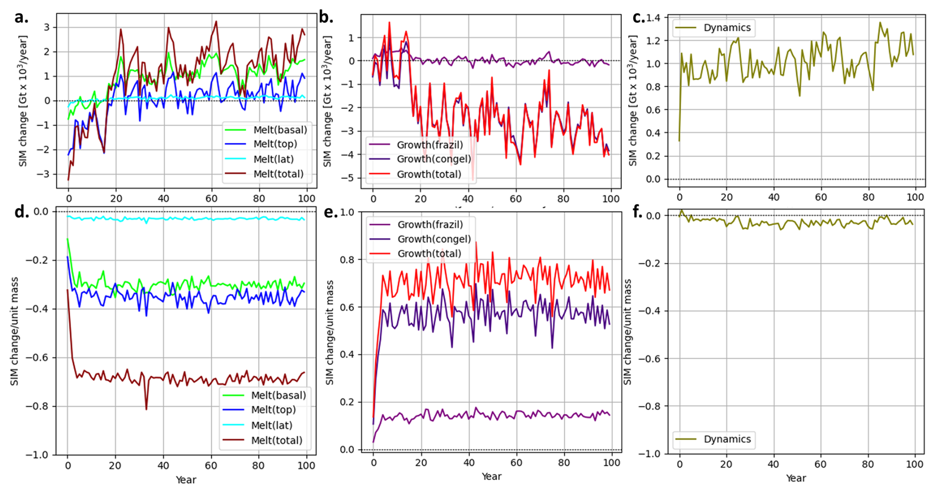
Figure A1 Timeseries as in Fig. 8 with additional diagnostics. Additional diagnostics are: (a, d) “melt” variables: basal melt, top melt and lateral melt; (b, e) “growth variables”: frazil and congelation growth; (c, f) mass change due to dynamics. Variables in (a–c) are calculated identically to Fig. 8a, and (d–f) are calculated identically to Fig 8b.

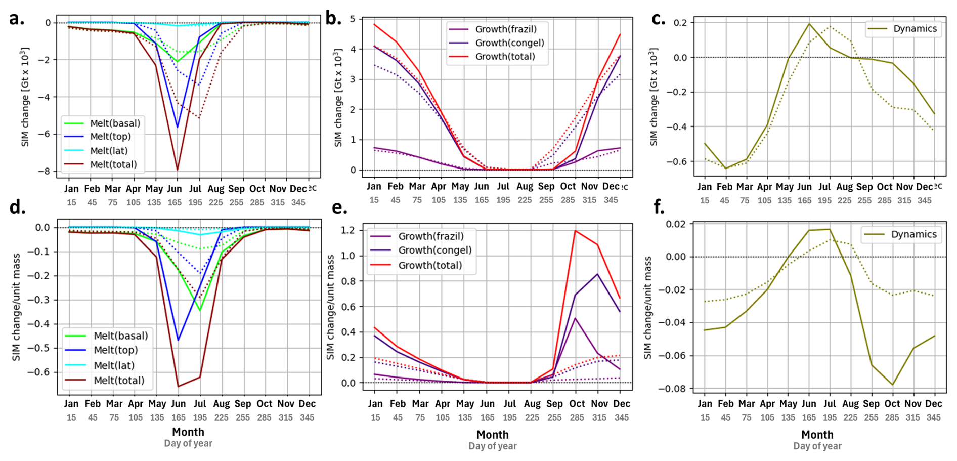
Figure A2 Monthly climatologies for abrupt-127k and piControl with additional ice budget diagnostics. HadGEM3 uses a 360 d calendar, so along the x axis we show both the month and the central “day of the year” for the month in the 360 d calendar. All panels show results calculated from monthly model output over years 51–100 for abrupt-127k (solid line) and piControl (dotted line). Variables in (a–c) are calculated without normalisation, and in (d–f) are calculated and then normalised using the monthly SIM. Additional diagnostics are: (a, d) “melt” variables: basal melt, top melt and lateral melt (b, e) “growth variables”: frazil and congelation growth (c, f) mass change due to dynamics.

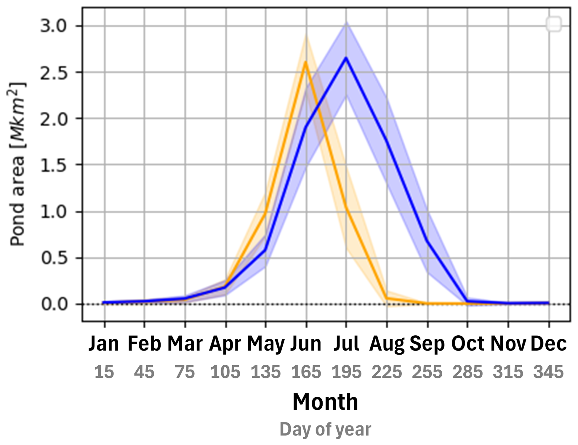
Figure A3 Monthly melt-pond climatology. Total melt-pond area, calculated using years 51–100 of both runs. Result from abrupt-127k (orange) and piControl (blue). HadGEM3 uses a 360 d calendar, so along the x axis we show both the month and the central “day of the year” for this month in the 360 d calendar.

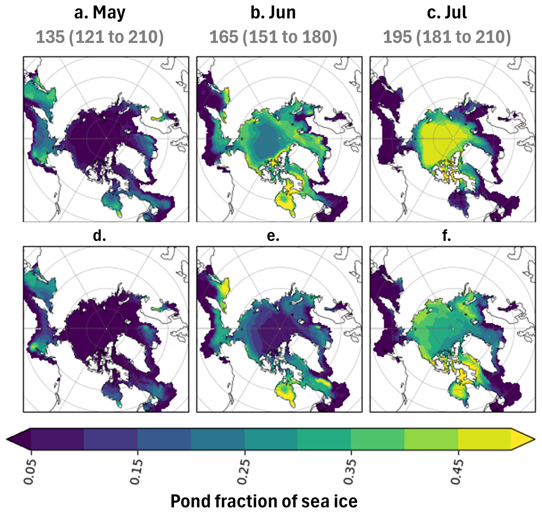
Figure A4 Mean monthly pond-covered fraction of sea ice, over years 51–100 of (a-c)  abrupt-127k and (d-f) piControl simulations. HadGEM3 uses a 360 d calendar, so along the x axis we show both the month and the central “day of the year” (day range in brackets) for this month in the 360 d calendar.

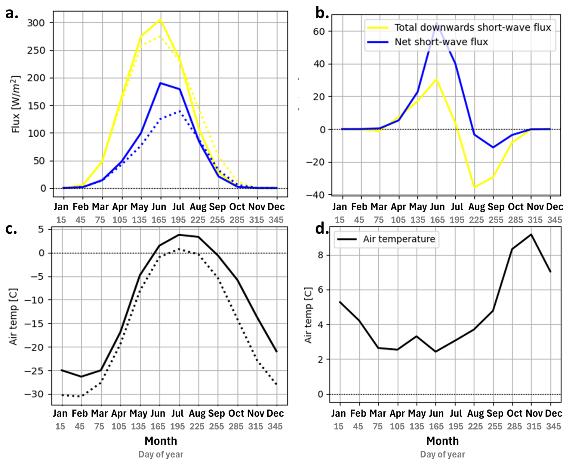
Figure A5 Short-wave radiation and surface air temperature for abrupt-127k and piControl: (a, c) Monthly abrupt-127k (solid) and piControl (dotted) climatologies and (b, d) monthly abrupt-127k – piControl anomaly for (a, b) total downwelling short-wave radiation (yellow) and net downwards short-wave radiation (blue) at the surface, and (c, d) surface air temperature. All variables calculated as long-term mean over years 51–100 of abrupt-127k and piControl runs, over the central Arctic: 70–90° N, with no land mask applied. HadGEM3 uses a 360 d calendar, so along the x axis we show both the month and the central “day of the year” for this month in the 360 d calendar.

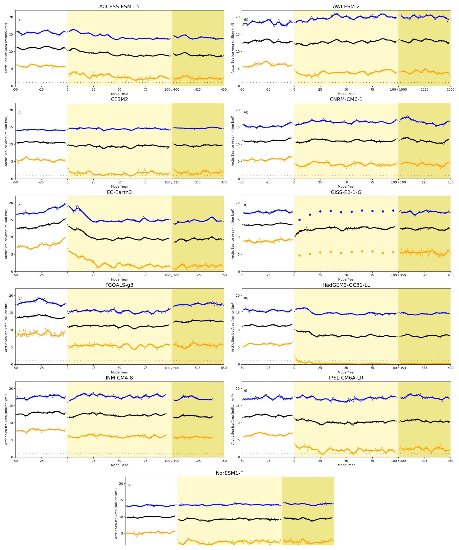
Figure A6 Multi-model evolution of sea ice area. (a–k) Per model breakdown of the data shown in Fig. 2, showing evolution of the annual monthly maximum (blue), average (black) and minimum sea ice area (orange) (after Diamond et al., 2021). Thicker lines show a 5-year running mean. Orange dotted lines represent a SIA of 1 × 10⁶ km², below which the Arctic is considered sea ice free. For (f), dots show a decadal average due to data limitations.

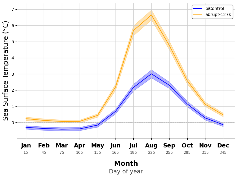
Figure A7 Seasonal cycle of Arctic (70–90° N) sea surface temperature (tos) averaged over years 51–100 for piControl and abrupt-127k.

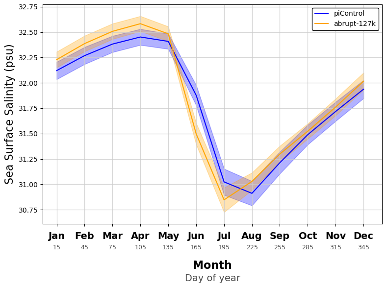
Figure A8 Seasonal cycle of Arctic sea surface salinity (sos) averaged over 70–90° N and years 51–100 for piControl and abrupt-127k.

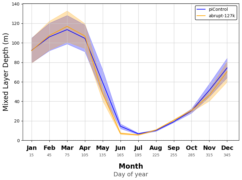
Figure A9 Seasonal cycle of Arctic mixed layer depth (mlotst) averaged over 70–90° N and years 51–100 for piControl and abrupt-127k.

Appendix B: Tier 2 experiments

Table B1 Experimental set-up – forcings and boundary conditions for the Tier 2 abrupt-127k simulations.

In addition to the Table 1, where groups have the resources required, we recommend two further abrupt-127k experiments (Table B1).

Tier 2: abrupt-127k-veg. Vegetation changes, including forest and tundra expansion in Canada and Greenland can lead to greater warming and ice loss during the Last Interglacial, compared with pre-industrial land cover (Sommers et al., 2021). For this reason we recommend, as a Tier 2 abrupt-127k experiment, that modelling groups switch between prescribed and interactive vegetation or develop Last Interglacial prescribed vegetation using an offline vegetation model, e.g. BIOME4 as in Otto-Bliesner et al. (2020), to permit the isolation and analysis of vegetation-specific feedbacks on the Arctic. Use of PaleoCalAdjust software (see also below) may be helpful in the analysis of seasonal vegetation-changes.

Tier 2: lig127k. Whilst the primary Arctic sea ice area change associated with 127k forcings occurs within 50 years (Fig. A6), further ocean–atmosphere–sea ice changes occur between 300 to 1000 years, after the imposition of the 127k forcings (Otto-Bliesner et al., 2021). Given groups may wish to compare their output to wider 127k observations, groups may also find it useful to extend their initial 100-year runs until they reach quasi-equilibrium. This would enable them to have also completed the PMIP4/7-lig127k, fully spun-up, 127k experiment. See also Otto-Bliesner et al. (2017, 2021).

The lig127k permits groups to further model responses to changes in orbital forcing, greenhouse gases, ice sheets, and feedbacks within the climate system (Otto-Bliesner et al., 2017). By benchmarking output against reconstructed temperatures, hydrology, sea ice, ice sheets, and ocean circulation during past warm climates, groups can further (i) assess model skill and structural uncertainty, (ii) improve understanding of key climate feedbacks and regional responses, and (iii) increase confidence in future climate projections under continued warming. In particular, the lig127k and other PMIP interglacials simulations provide critical insight into polar amplification, ice-sheet stability, sea-level sensitivity, and the behaviour of the coupled atmosphere–ocean–cryosphere system under climates comparable to or warmer than today (Otto-Bliesner et al., 2017).

Note that PaleoCalAdjust software has been developed to re-aggregate variables on normal CMIP “fixed-length” months onto “fixed-angle” months (Bartlein and Shafer, 2019). This may be useful for further analysis using seasonal or monthly averages from these extended lig127k simulations. If groups wish to investigate calendar adjustment, it is helpful to output the optional subset of daily sea ice variables (Table 3); this allows different monthly aggregation approaches to be tested, and also facilitates the use of the PaleoCalAdjust software.

Appendix C: Methods: A recipe for abrupt-127k output

This Appendix contains further technical details which may be useful to groups who undertake the recommended abrupt-127k analyses, alongside additional optional analyses.

C1 Overview of additional analyses

The optional additional analyses are shown in Appendix figures: Figs. A1 to A5 provide additional diagnostics and climatological insights. Figure A1 extends the timeseries analysis shown in Fig. 8 by including key ice budget diagnostics, specifically basal, top, and lateral melt, frazil and congelation growth, and mass changes due to dynamics. Figure A2 presents monthly climatologies of ice budget components and their comparison with piControl over years 51–100. Figures A3 and A4 focus on melt-pond dynamics, showing the pond-covered fraction of ice and total melt-pond area, comparing abrupt-127k and piControl simulations. Figure A5 examines surface energy balance terms.

These additional figures are less critical than the main figures and analyses in the main text. However, for studies involving other sea ice processes, particularly prognostic melt ponds, groups may find it useful to examine these additional ice budget diagnostics, including melt pond areas, using monthly (or, if possible, daily) total melt pond area. Given the strong radiation forcing at 127 ky, a larger spring melt pond area and earlier melt onset are expected for abrupt-127k (Guarino et al., 2020; Diamond et al., 2021).

C2 Further details, useful for the characterisation of the abrupt-127k sea ice state (O1)

Ice-related quantities shown (ice concentration, mass, pond-related quantities, and growth- and melt-related quantities for the sea ice budgets) are calculated using Northern Hemisphere grid-cells. We indicate the relevant sea ice variables from Table 3 in underlined italics.

Sea ice area (SIA) is the sum of sea ice concentration siconc_i (siconc) over all grid-cells, weighted by cell area a_i (areacello)

$$\begin{array}{}\text{(C1)}& \text{SIA}=\sum _i^N{\text{siconc}}_{\mathrm{i}}\times a_{\mathrm{i}}.\end{array}$$

Sea ice volume (SIV) is the area-weighted mean of the volume per unit area h_i (sivol) over all grid-cells, or equivalently if using ice thickness sithick_i (sithick) over ice-covered portion of grid-cell only:

$$\begin{array}{}\text{(C2)}& \text{SIV}=\sum _i^N{h}_{\mathrm{i}}\times a_{\mathrm{i}}=\sum _i^N{\text{sithick}}_{\mathrm{i}}\times ({\text{siconc}}_{\mathrm{i}}\times a_{\mathrm{i}})\end{array}$$

Following Keen et al. (2021) and Notz et al. (2016), we recommend using sea ice mass (SIM) instead of SIV. SIM is calculated from the ice mass per unit area in each grid-cell m_i (simass)

$$\begin{array}{}\text{(C3)}& \text{SIM}=\sum _i^N{m}_{\mathrm{i}}\times a_{\mathrm{i}}\end{array}$$

C3 Further details, useful for the Arctic abrupt-127k surface energy budget calculations (O3)

We indicate the relevant atmospheric variables from Table 2 in underlined italics.

The atmospheric quantities (surface air temperature tas and energy budgets) should be calculated over the central Arctic: 70–90° N, with no land mask applied, as in Kageyama et al. (2021). Note this does include some northern land masses, including the northern half of Greenland.

For each O3 variable, use an area-weighted average over this region (e.g. Fig. 7). `Net downwards' long-wave and short-wave fluxes shown in Figs. 7 and A5 are equal to the downwelling flux minus the upwelling flux (for long-wave, respectively rlds and rlus; for short-wave, rsds and rsus).

Total albedo can be estimated from downwelling SW_downwelling (rsds) and upwelling SW_upwelling (rsus) short-wave flux at the surface as

$$\begin{array}{}\text{(C4)}& \begin{array}{rl}\text{albedo}=& \mathrm{1}-({\text{SW}}_{\text{downwelling}}-{\text{SW}}_{\text{upwelling}})\\ & /{\text{SW}}_{\text{downwelling}}\end{array}\end{array}$$

and then an area-weighted average taken to plot the climatologies (e.g. Fig. 7b).

C4 Further details, useful for ice budget melt-growth-dynamic terms (O4)

Ice-related quantities shown (ice concentration, mass, pond-related quantities, and growth- and melt-related quantities for the sea ice budgets) are calculated over Northern Hemisphere grid-cells.

The most important quantities for basic analysis of the ice budgets are total melt, total growth, and dynamics, but the other diagnostics shown can aid interpretation of the results.

Analysis of ice mass changes in abrupt-127k due to melt, growth, and ice dynamic terms should be carried out using the sign conventions where mass increase (e.g. due to growth or convergence) is positive and mass decrease (e.g. due to melt or divergence) is negative (c.f Keen et al., 2021). Therefore, when the abrupt-127k is compared to the piControl simulation, positive values indicate changes that increase SIM (and SIV) in abrupt-127k relative to piControl, and negative values indicate changes that reduce SIM (and SIV).

Following SIMIP, the use of SIM, and mass change per month, is recommended (Notz et al., 2016; Keen et al., 2021). In this manuscript, we calculated SIM and mass change per month by multiplying SIV and volume change per month by the ice density 917 kg m⁻³: the ice density is fixed in most models, and otherwise varies very little (Keen et al., 2021).

Where required, rather than normalising results using SIA (as in Fig. 10c of Keen et al., 2021), we recommend normalising using the SIM. This is because the difference between the abrupt-127k and piControl simulations for SIM is fairly consistent year-round (see Fig. 5c), whereas there is strong seasonality in the difference in SIA due to the seasonal nature of the forcing (Figs. 3 and 5b).

The three quantities necessary for the basic ice budget analysis are: total growth, total melt, and ice change due to advection/dynamics. These can be estimated from basic model diagnostics as shown below. We estimated the change in ice thickness Δh_process,i due to a given process in each grid-cell using the dominant terms:

$$\begin{array}{}\text{(C5)}& {\displaystyle }& {\displaystyle }\mathrm{\Delta }{h}_{\text{melt},\mathrm{i}}=\mathrm{\Delta }{h}_{\text{basal\hspace{0.17em}\hspace{0.17em}melt},\mathrm{i}}+\mathrm{\Delta }{h}_{\text{top\hspace{0.17em}\hspace{0.17em}melt},\mathrm{i}}+\mathrm{\Delta }{h}_{\text{lateral\hspace{0.17em}\hspace{0.17em}melt},\mathrm{i}}\text{(C6)}& {\displaystyle }& {\displaystyle }\mathrm{\Delta }{h}_{\text{growth},\mathrm{i}}=\mathrm{\Delta }{h}_{\text{frazil},\mathrm{i}}+\mathrm{\Delta }{h}_{\text{congel},\mathrm{i}}\end{array}$$

For abrupt-127k output, we recommend using mass change Δm_process,i due to each process (underlined subscripts) _sidmassx indicate the variable from Table 3). Equivalently to above, we estimate using the dominant terms

$$\begin{array}{}\text{(C7)}& {\displaystyle }\begin{array}{rl}\mathrm{\Delta }{m}_{\text{melt},\mathrm{i}}=& \mathrm{\Delta }{m}_{\text{sidmassmeltbot},\mathrm{i}}+\mathrm{\Delta }{m}_{\text{sidmassmelttop},\mathrm{i}}\\ & +\mathrm{\Delta }{m}_{\text{sidmassmeltlat},\mathrm{i}}\end{array}\text{(C8)}& {\displaystyle }\begin{array}{rl}\mathrm{\Delta }{m}_{\text{growth},\mathrm{i}}=& \mathrm{\Delta }{m}_{\text{sidmassgrowthwat},\mathrm{i}}\\ & +\mathrm{\Delta }{m}_{\text{sidmassgrowthbot},\mathrm{i}}\end{array}\end{array}$$

We do not include other terms (e.g. contribution from sublimation and snow ice formation) in these estimates, as Keen et al. (2021) showed these are much smaller in the Arctic.

If using thickness or volume-based quantities, the total volume change ΔSIV_process due to each process per month should be calculated as the area-weighted sum of the ice thickness change for each grid-cell due to this process.

As above, we recommend using mass change rather than volume change for simplicity, e.g. for mass change due to melt ΔSIM_melt:

$$\begin{array}{}\text{(C9)}& \mathrm{\Delta }{\text{SIM}}_{\text{melt}}=\sum _i^N\mathrm{\Delta }{m}_{\text{melt},\mathrm{i}}\times a_{\mathrm{i}}\end{array}$$

Total melt-pond area MPA, and mean pond fraction of ice $\stackrel{\mathrm{‾}}{\text{mpc}}$, can also be of interest (Figs. A2 and A3). These are calculated using pond fraction of the ice simpconc_i (simpconc from Table 3)

$$\begin{array}{}\text{(C10)}& {\displaystyle }& {\displaystyle }\text{MPA}=\sum _i^N{\text{simpconc}}_{\mathrm{i}}\times ({\text{siconc}}_{\mathrm{i}}\times a_{\mathrm{i}})\text{(C11)}& {\displaystyle }& {\displaystyle }\stackrel{\mathrm{‾}}{\text{mpc}}={\displaystyle \frac{\text{MPA}}{\text{SIA}}}\end{array}$$

C5 Further details, Arctic Ocean near-surface stratification

To characterise upper-ocean adjustments in the abrupt-127k simulation, we include additional seasonal diagnostics of Arctic Ocean near-surface temperature and salinity structure (Figs. A7–A9). These diagnostics use monthly data from years 51–100 and are calculated as area-weighted averages over 70–90° N, with no land mask applied, consistent with the surface energy budget calculations described above.

We indicate the relevant ocean variables from the baseline_monthly output in underlined italics.

Sea surface temperature (SST; tos) provides a measure of the upper-ocean thermal state. Sea surface salinity (SSS; sos) reflects freshwater forcing and stratification changes. Mixed layer depth (MLD; mlotst) characterises the vertical extent of active mixing and therefore the strength of near-surface stratification.

During the melt season (May–September), abrupt-127k is characterised by substantially warmer SSTs, slightly fresher surface waters, and a consistently shallower mixed layer relative to piControl. Together, these features indicate enhanced near-surface stratification consistent with reduced sea-ice cover and increased surface heating. Outside the melt season (January–April), differences are small: abrupt-127k shows marginally higher SSS and a slightly deeper mixed layer, but anomalies remain weak.

These ocean diagnostics demonstrate that Arctic stratification changes in abrupt-127k are strongly seasonally focused and closely aligned with the simulated summer sea-ice reductions described in the main text.