Interpolating station quantile biases for tropospheric ozone MDA8 bias correction

Chemistry transport models (CTMs) consistently exhibit systematic errors in ozone concentrations, which can be partly compensated by bias correction. There are several bias correction strategies suitable for using station data, but they are likely to introduce statistical artifacts when applied at high resolution. We propose a new bias correction strategy based on parametric interpolation of quantile biases (PIQB) suitable for high resolution simulations, which is designed to avoid such artifacts. In this study, we evaluate and compare the performance of our strategy with other older strategies with a focus on ambient maximum daily 8 h average ozone concentrations (MDA8). Our experimental setup consisted of two simulations from the CTMs WRF-Chem and CAMx at horizontal resolution of 9 km within the time period of 2007–2016 and 165 ground-based stations in central Europe. Our results show that each strategy brings the simulated MDA8 closer to observations, but PIQB performs the best in terms of mitigating systematic errors while retaining the modeled fine resolution structure of spatial variability. We conclude that out of the considered strategies, PIQB is the most suitable one for bias correction at high resolution, suggesting its possible applications for correcting climate projections of ozone MDA8.

1 Introduction

Tropospheric ozone belongs among important gas-phase pollutants, having negative impacts on health of both fauna and flora (Da et al., 2022; Gu et al., 2023; Pozzer et al., 2023). Because of that, it is desired by both the scientific community and policy-makers to study the long-term evolution of its concentrations, including the interactions among air quality and the changing climate (Racherla and Adams, 2008; Doherty et al., 2017; Archibald et al., 2020). The chemical production of ozone is initiated by photochemistry, and so the dominant influence upon its concentrations is the budget of its precursors, i.e., oxides of nitrogen (NO_x) and volatile organic compounds (VOCs) as well as the amount of sunlight, temperature and humidity (Seinfeld and Pandis, 1998). That is mostly why projecting ozone concentrations into the future is burdened with uncertainty, as mitigating the anthropogenic NO_x budget may not be enough to compensate for the influence of the rising temperature and humidity (Colette et al., 2015).

To model the complex interactions among chemical species and other components of the climate system, global chemistry models can be used (e.g., Emmons et al., 2020; Sukhodolov et al., 2021). However, their relatively coarse resolution limits their performance in assessing regional ozone burdens simply due to the inability to fully represent subgrid-scale effects, such as local sources of pollution or fine orographical features. Such limitations often result in biases or other types of systematic errors when compared to station observations (Rieder et al., 2015; Revell et al., 2018; Liu et al., 2022). To obtain information at finer resolutions, regional chemistry-transport models (CTMs) nested into global models are widely used, as they are capable of taking into account the transport of many different species from their sources along with their chemical interactions within the atmosphere (Grell et al., 2005; ENVIRON, 2018). Despite including features unresolved by global models and providing outputs at resolutions of units of kilometers, CTMs are still not perfect and exhibit systematic errors as well (Mar et al., 2016; Karlický et al., 2017, 2024; Prieto Perez et al., 2025). Such model errors compared to measurements (which generally serve as the ground truth) are therefore an inherent feature of air quality simulations.

Luckily, the inevitability of errors can be at least partly compensated by postprocessing, namely by statistical procedures known as bias correction (e.g., Rieder et al., 2015; Rahmani et al., 2017; Abdelmoaty et al., 2025; Im et al., 2025), which adjust the model data to better fit the corresponding observations. In its general form, bias correction requires three inputs, which are observations, modeled data corresponding to the observations and modeled data to be corrected. Its main motivation is the application on projections through the assumption that the systematic errors arise from the model itself and are therefore identical in the projection and a historic run using input data generated by the same methodology. This assumption yields another source of uncertainty, because it depends on the definition of the systematic error, which may be assumed different across various bias correction strategies (Ugolotti et al., 2023; Staehle et al., 2024), on top of which, there is evidence from Liu et al. (2022) that biases differ with chemical environment and hence will potentially be different between a projection and a present-day simulation. Additionally, different sources of observations can be used for bias correction, and so the result and performance of such corrections may depend on the choice of reference data as well (Schnell et al., 2014; Staehle et al., 2024). In this study, we explore using ground based station measurements, as they represent the actual ground-level immissions.

As there are mostly studies applying bias correction of ozone concentrations using station data to model grids at coarse resolution (e.g., Schnell et al., 2014; Rieder et al., 2015), we aim to address their use for finer resolution climate simulations to demonstrate the possibility and to contribute to this research area. On the other hand, operational air quality forecasts use some form of bias correction on a routine basis (e.g., Neal et al., 2014). And so, regarding postprocessing of a regular model grid using station data, the task must be approached from the following perspectives: (i) the choice of statistical procedure to correct a single model time series (i.e., correcting corresponding datasets) and (ii) the strategy for extrapolating the outreach of such a procedure into the regular grid (i.e., correcting non-corresponding datasets).

To address (i), based on a recent comparison performed by Staehle et al. (2024), a procedure called quantile mapping (QM) detailed by Rieder et al. (2015) performs satisfyingly well compared to other methods (and is commonly used for other variables as well, e.g, precipitation; Abdelmoaty et al., 2025), and thus shall be considered in this study. The key principle of QM dwells in unifying each inter-quantile range (within a fixed set of quantiles) and its relative position of the modeled and observed data separately, therefore taking into account the possibility of having different biases in different parts of the modeled probability density function (PDF). This is especially crucial in the case of correcting ozone concentrations, as the statistical systematic errors may emerge naturally from the discrepancies between the modeled and observed PDFs (Karlický et al., 2024).

From the perspective of (ii), the task is to utilize the local information contained within the station sites in other parts of the model domain. In other words, we wish to somehow represent or to generalize the station measurement outside of the few model grid-cells to obtain a seamless dataset which would be directly comparable to the modeled data in each grid-box. It should not be surprising that in such a task many problems emerge. Most importantly, if done with an insufficient care, there is a risk of corrupting the simulation physics with statistical artifacts, as also demonstrated in this paper.

This study proposes a strategy of bias correction suitable for fine resolution simulations and usage of ground-based station data, which avoids introducing statistical artifacts and returns a seamless correction. Furthermore, both a qualitative and a quantitative comparison will show the differences between our proposed strategy and others found in literature, as well as the impact of the choice of a strategy upon the spatial distribution of a policy-relevant metric.

2 Data and methods

Further follows the description of three different strategies how to represent station data in the whole domain for the purposes of bias correction and the description of our experimental setup in terms of used data and methods. Each of the bias correction strategies has certain advantages as well as limitations. The strategies considered in this study are (i) statistically adjoint PDFs, (ii) direct interpolation of station data and (iii) parametric interpolation of quantile biases (PIQB).

2.1 Adjoint PDFs

The following strategy is the simplest one to implement and has been shown to be efficient in the conditions of coarse-resolution simulations (Rieder et al., 2015). From the statistical point of view, the idea is to treat all observations contained within the domain as random realizations of an experiment, which serve as the observational input for QM. Then, only those grid-cells containing stations are used as the corresponding modeled data.

Then, these two inputs form two PDFs which are compared to each other, which serves as the training process for QM. The relationship between the PDFs is then extrapolated to the PDF of the rest of the domain, i.e., the full extent of modeled data within the domain. This step assumes representativeness of the limited number of stations, as well as of the corresponding biases, for the whole domain.

The main advantage of this strategy is its computational efficiency and that there is no need for any kind of interpolation. It works very well at coarse resolutions where most model grid-cells contain at least one station and in the cases where the model correctly resolves large-scale spatial variability. However, in the cases of a thin station coverage, fine resolution or poorly resolved spatial distributions by the model, the results may contain statistical artifacts.

To explain such artifacts, let us consider an example where the observations do not cover areas with extreme values of the modeled data, which is typical for fine-resolution simulations. If the comparison of PDFs at station sites finds that the model underestimates the width of its PDF, this strategy would then stretch the domain-wide modeled PDF, making minima lower and maxima higher regardless of their physical plausibility. Similarly, any errors in the large-scale spatial variability would be even more highlighted, as the strategy does not consider the possibility of having different biases throughout the domain.

2.2 Interpolation of observations

A different approach would be to truly rely on station data and their representativeness for the nearest neighboring grid-boxes. Such a strategy has been used to generate gridded datasets of observations (at a correspondingly coarse resolution) to correct the uncertainties of global models by Schnell et al. (2014).

The interpolation of station data into a regular model grid can be conducted using a weighted average with an appropriate weighting function, such as inverse distance weighting (IDW), i.e.,

$$\begin{array}{}\text{(1)}& {\stackrel{\mathrm{̃}}{w}}_k(d_k,\mathit{\beta })={\displaystyle \frac{\mathrm{1}}{d_k^{\mathit{\beta }}}},\end{array}$$

where d_k is the distance to the kth station and β is the interpolation parameter. For a total number of stations N, these weights are then normalized to have a unit sum using the following formula

$$\begin{array}{}\text{(2)}& w_k(d,\mathit{\beta })={\displaystyle \frac{{\stackrel{\mathrm{̃}}{w}}_k(d_k,\mathit{\beta })}{\sum _{i=\mathrm{1}}^N{\stackrel{\mathrm{̃}}{w}}_i(d_i,\mathit{\beta })}}\end{array}$$

and are used to obtain the resultant interpolated observation O in an arbitrary point p as

$$\begin{array}{}\text{(3)}& O^p=\sum _{k=\mathrm{1}}^N{w}_k{O}^k.\end{array}$$

The parameter β can be optimized based on various criteria, e.g., minimizing some residual validation statistic in cross-validation (Schnell et al., 2014).

The strategy would then be to interpolate the measurements into the model grid and perform bias correction in each grid-box individually. This way, the spatial distribution of observations is reflected in the corrected simulations, which adds the information about the large-scale spatial variability from observations compared to the previous strategy.

On the other hand, while the large-scale features may be resolved well, applying this strategy onto fine resolution simulations may result in suppressing some fine resolution model features in model grid-cells neighboring to the stations. This means that an area with locally lower ozone concentrations resolved by the model surrounded by stations measuring generally higher concentrations will be lost after the interpolation.

In other words, if a large grid-box contains multiple stations, its mean climate corresponds well to the mean climate of the stations. However, in the opposite situation when multiple fine grid-boxes are supposed to be represented by one station, this strategy fails, because the model provides more information about the spatial variability within the domain.

2.3 Parametric interpolation of quantile biases

Lastly, we propose a new strategy to address the above mentioned problems, which is fairly similar to the previous one, but we perceive it as a hybrid of both the strategy of adjoint PDFs and the interpolation of observations. The key assumption is that the physics and the chemistry of the atmospheric processes in terms of spatial distribution are well represented within the simulations and that the only issue is with the overall bias and mismatch in PDF shapes, i.e., the maxima and minima may not be representative enough within the model.

We can expand the issues with bias and variability by fusing them into one which we shall call quantile bias. Consistently with the mechanism of QM, we can assume that each quantile is biased differently. Additionally, we may even assume that the spatial distribution of quantile biases is suitable for interpolation from stations.

Considering the above mentioned assumptions, let us define quantile bias $B_q^k$ of a quantile q at a station k as follows,

$$\begin{array}{}\text{(4)}& B_q^k=M_q^k-O_q^k,\end{array}$$

where $O_q^k$ and $M_q^k$ are the qth quantile of the kth station of observations and its corresponding model value respectively. We shall interpolate this quantity from stations to an arbitrary point p using a weighted average with weighting functions w_k, i.e.,

$$\begin{array}{}\text{(5)}& B_q^p=\sum _{k=\mathrm{1}}^N{w}_k{B}_q^k.\end{array}$$

By expanding $B_q^k$ in Eq. (5) by their definition in Eq. (4) and rearranging the symbols, we obtain

$$\begin{array}{}\text{(6)}& O_q^p=M_q^p+\sum _{k=\mathrm{1}}^N{w}_k\left(O_q^k-M_q^k\right),\end{array}$$

which shall serve as the interpolation formula to obtain pseudo-observations $O_q^p$ in the regular model grid.

From Eq. (6) it should be somehow apparent why we claim this strategy to be a hybrid of the two previously presented ones. On one hand, it takes into consideration the spatial variability of the observed data, but on the other hand uses the model data as a support to fill in the blank space in between the stations. This feature is depicted in Fig. 1 where the left hand side figure illustrates the definition of B_q and the middle figure compares the interpolation of observations $O_q^k$ (which only mimics the properties of observations) and the interpolation of $B_q^k$ (which considers both observed and simulated data).

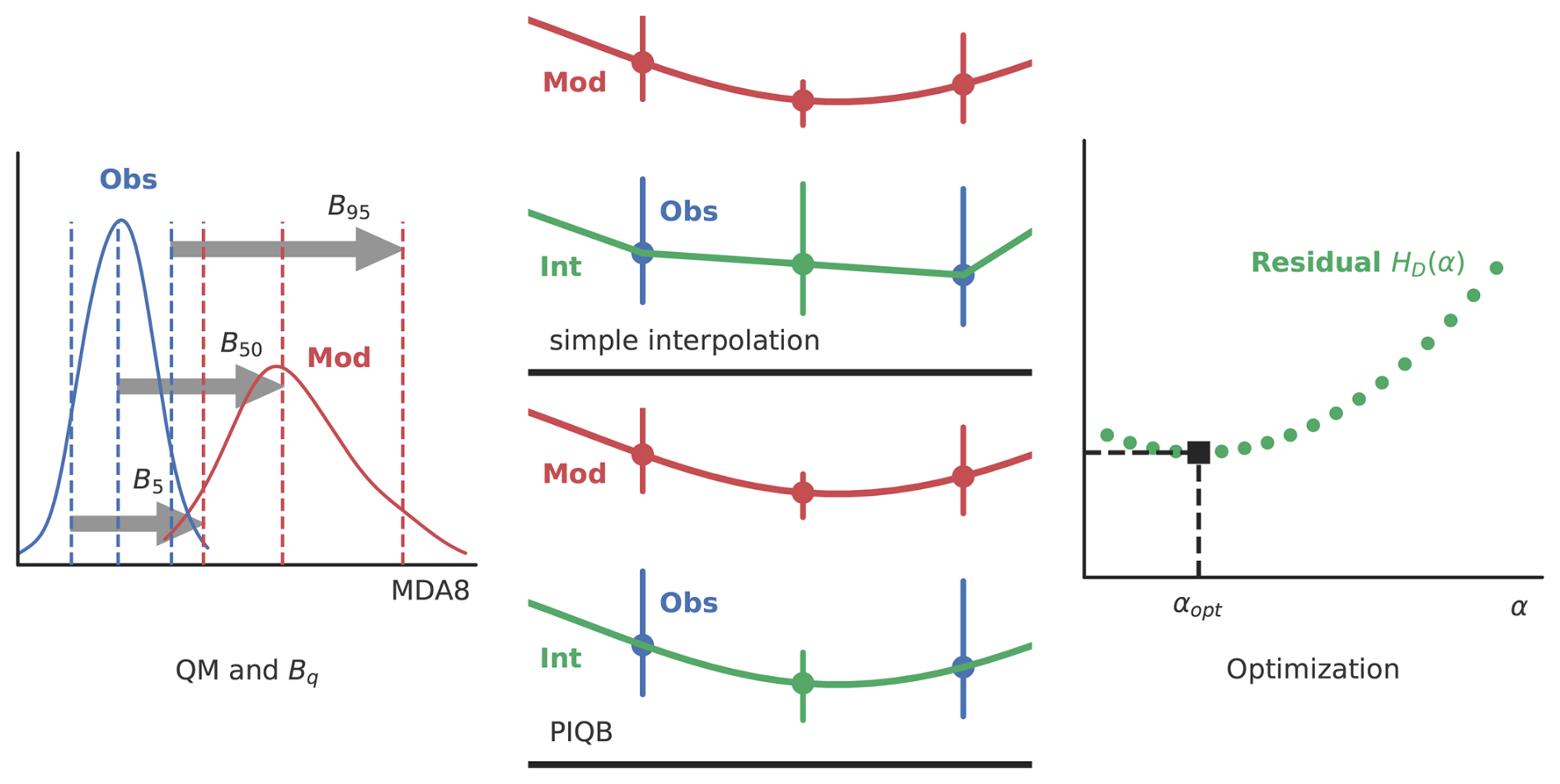
Figure 1 A methodological flowchart of interpolating bias correction strategies. An illustration of positive sign quantile biases is depicted in the left figure with the observed (Obs, blue) and modeled (Mod, red) PDFs of MDA8. In the middle figure, there is a comparison of interpolating observations (top) and quantile biases (bottom) with the observed (Obs, blue) and modeled boxplots (Mod, red) and the resultant interpolations (Int, green). Finally, the optimization process is illustrated on the right with the residual error H_D(α) (green, described further in text) as a function of the interpolation parameter and a marked optimum (black square).

A similar idea has already been tested with a certain degree of success by Rahmani et al. (2017) in terms of absolute bias interpolation. The difference is that their work was focused on the biases in forecast models and the definition of quantile biases would be complicated with the limited amount of data. For this reason, their setup was not suitable for expanding to bias correction of climate projections, simply because longer simulated periods would be necessary.

The procedure then continues in the same way as in the previous strategy, which is the correction of each grid-box individually using QM. This also implies that only the pseudo-observed quantiles needed for QM are necessary to obtain from the interpolation by Eq. (6), which significantly reduces its computational demand.

The weights w_k can once again be chosen as IDW in Eq. (1), but that is not a choice we would recommend. Although IDW is an exact interpolator, it is prone to errors (e.g., Achilleos, 2008; Gentile et al., 2012; Ohlert et al., 2023). Instead, we propose a smoother option on a similar basis, which is a gaussian weighting function, i.e.,

$$\begin{array}{}\text{(7)}& {\stackrel{\mathrm{̃}}{w}}_k(d_k,\mathit{\alpha })=e^{-\mathit{\alpha }{d}_k^{\mathrm{2}}},\end{array}$$

where α is an interpolation parameter and the weights should be once again normalized to yield unit sum in an analogy to Eq. (2). A parameter figures in both presented weighting options, which allows for an optimal setting of the interpolation. Such a process is detailed in further sections. Therefore, we shall name this overall strategy the Parametric Interpolation of Quantile Biases (PIQB).

2.4 Model data and observations

Following the description of the statistical procedures, we shall now introduce the data used in this study. Starting with model data, we consider outputs of two CTMs: (i) the Weather Research Forecasting model with online coupling to chemistry (WRF-Chem, v. 4.0.3; Grell et al., 2005) and (ii) Comprehensive Air Quality Model with Extensions (CAMx, v. 6.50; ENVIRON, 2018). CAMx was offline coupled to WRF meteorology using the wrfcamx meteorological preprocessor, i.e., without considering feedbacks on model radiation (Huszar et al., 2012). The simulations were conducted in the period of 2007–2016 with horizontal resolution of 9 km in the domain of Central Europe with a spatial extent depicted in Fig. 2, consisting of 190 × 166 grid-boxes in the meridional and zonal direction respectively. Our analysis is based exclusively on maximal diurnal averages of 8 h of ozone concentrations (MDA8), which required a preprocessing of the original hourly output. The overall setup is identical to the one used in the study by Karlický et al. (2024), to which the reader is kindly referred to for further information.

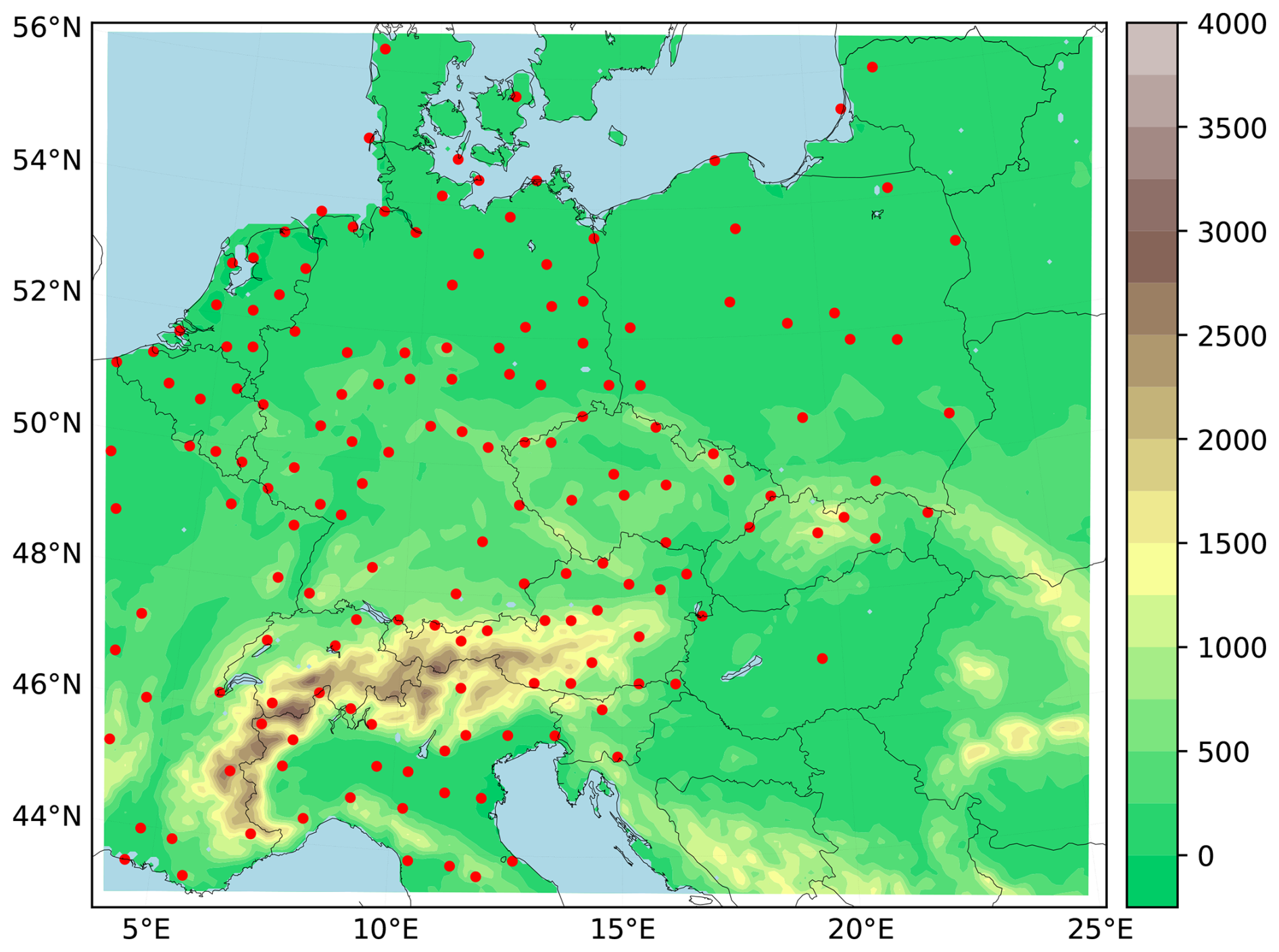
Figure 2 The model domain of Central Europe with topography. Red dots mark all of the 165 stations considered for the analyses and corrections performed in this study.

From the simulations used by Karlický et al. (2024), we consider those using meteorological boundary conditions (BCs) taken from the ERA-interim reanalysis (Dee et al., 2011) and chemical BCs taken from the global model SOlar Climate Ozone Links (SOCOL; Sukhodolov et al., 2021). This choice is motivated by the possibility of using those simulations to calibrate corrections of climate projections, as this is the main purpose of bias correction. The possibility stems from the fact showed by Karlický et al. (2024) that the meteorological BCs only influence correlation, but not the overall bias, while chemical BCs only impact biases, and so this combination would correct the systematic errors in future climate simulations which rely on global model data.

Moving to the reference data, station measurements from a sub-selection of rural background stations of the European Environmental Agency (EEA) station network were taken and the original database is freely accessible at https://eeadmz1-downloads-webapp.azurewebsites.net/ (last access: 12 December 2025). Our final selection of stations was chosen based on an algorithm described by Karlický et al. (2024): first, only those stations with measurements covering at least half of the simulation period were selected from the total available stations. Then, for each of the remaining 298 stations, a basic quality-control check was made by counting the number of measured hourly concentrations lower than the seasonal mean decreased by 2.5-times the standard deviation of the hourly data. Several stations spiked with an unprecedented number of such values (in the order of thousands within two consecutive years) and were thus removed from the list as we would not expect such rural stations to be representative for their corresponding grid-boxes within the simulations of 9 km resolution. Lastly, an iterative elimination algorithm was used on the remaining 271 stations to homogenize their density based on their relative position, removing a station with the lowest mean distance to its 2 closest neighbors in each step. This way, the final number of 165 stations remained on the list and are marked in Fig. 2 by red dots. The spatial homogeneity of the station network is important for both the objectivity of the validation of the model performance and for the prevention of overfitting statistical models.

2.5 Methods of validation

Let us now proceed to the description of the optimization and evaluation process. For the optimization, we adopted cross-validation and its purpose is two-fold, as it allows us to optimize the interpolation parameters as well as to quantify the ability of each strategy to represent the station information in the model grid. In the context of climate simulations, the general standard for the purposes of climate analyses is to consider up to four distinct 3-months long climatological seasons (studies performed by, e.g., Huszar et al., 2012; Colette et al., 2015; Im et al., 2015; Rieder et al., 2015; Mar et al., 2016; Karlický et al., 2017, 2024; Staehle et al., 2024), but we are aware that this could potentially result in sharp discontinuous jumps at the boundaries of each season after the correction. That is why here the optimal values for the parameters α and β in Eqs. (7) and (1) were chosen for each month separately, meaning that the discontinuities in the corrected time series would be on one hand more frequent, but on the other hand less notable. Furthermore, to prevent overfitting, the data were divided into twelve 3-months long overlapping moving seasons in the full extent of the 10 years always with the middle month being the target period. This way, the corrected results may have a less accurate match to the observations (i.e., some quantiles used by QM to correct the middle month may belong to a different month), but simultaneously the corrections are smoother in time, meaning that adjacent calendar months are corrected similarly to each other, thus preserving at least a part of the modeled qualitative annual cycle.

For each moving season, a brute-force 1-out cross-validation algorithm was adopted, which we shall now explain. First, a station is chosen out of the N=165 stations considered, and removed momentarily. Then, the statistical correction within the chosen moving season is performed using the remaining N−1 stations with a chosen value of the parameter α. The results are validated on that one missing station only in the middle month to obtain a residual value of a certain validation statistic which we describe further.

This process is then repeated with the fixed value of α for all of the N stations. After that, the mean value of the chosen validation statistic is taken. Repeating this procedure for different values of α will return the empirical function of the dependence of the averaged residual validation statistic on the parameter α. The optimal value for α in each month is the minimizer of such a function for that given month.

As should be apparent, a suitable validation statistic for this task should be one that considers the overall match of the observed PDF f_O(x) and its corresponding statistical reconstruction f_M(x,α). Therefore, we chose the Hellinger distance (H_D;  Jeffreys, 1946) describing the mismatch of two PDFs in the following form,

$$\begin{array}{}\text{(8)}& H_{\mathrm{D}}\left(\mathit{\alpha }\right)={\displaystyle \frac{\mathrm{1}}{\mathrm{2}}}\underset{-\mathrm{\infty }}{\overset{\mathrm{\infty }}{\int }}{\left(\sqrt{f_{\mathrm{O}}\left(x\right)}-\sqrt{f_{\mathrm{M}}(x,\mathit{\alpha })}\right)}^{\mathrm{2}}\mathrm{d}x,\end{array}$$

where, in our case, the values of x would correspond to MDA8 of ozone, and H_D(α) is the empirical function to be minimized.

The existence of a global minimum of H_D(α) using normalized gaussian weights from Eq. (7) can be shown heuristically. Let us consider the extreme cases, i.e., (i) α=0 and (ii) α→∞. In the case (i), all stations would have the same normalized weights, i.e.,

$$\begin{array}{}\text{(9)}& \begin{array}{rl}& \forall k:{\stackrel{\mathrm{̃}}{w}}_k(d_k,\mathit{\alpha }=\mathrm{0})=e^{\mathrm{0}}=\mathrm{1}\\ & \Rightarrow \forall k:w_k(d_k,\mathrm{0})={\displaystyle \frac{e^{\mathrm{0}}}{{\sum }_{i=\mathrm{1}}^N{e}^{\mathrm{0}}}}={\displaystyle \frac{\mathrm{1}}{N}},\end{array}\end{array}$$

where the implied values of w_k follow from Eq. (2).

In the case (ii), only the station with the minimal distance to the interpolation point $d_m={min}_k{d}_k$ would have a non-zero weight, which follows from the following limit:

$$\begin{array}{}\text{(10)}& \begin{array}{rl}& \forall k:w_k(d_k,\mathit{\alpha }\to \mathrm{\infty })=\underset{\mathit{\alpha }\to \mathrm{\infty }}{lim}{\displaystyle \frac{e^{-\mathit{\alpha }{d}_k^{\mathrm{2}}}}{\sum _{i=\mathrm{1}}^N{e}^{-\mathit{\alpha }{d}_i^{\mathrm{2}}}}}\\ & =\underset{\mathit{\alpha }\to \mathrm{\infty }}{lim}{\displaystyle \frac{e^{-\mathit{\alpha }(d_k^{\mathrm{2}}-d_m^{\mathrm{2}})}}{\sum _{i=\mathrm{1}}^N{e}^{-\mathit{\alpha }(d_i^{\mathrm{2}}-d_m^{\mathrm{2}})}}}=\left\{\begin{array}{ll}\mathrm{1}& \text{if}{d}_k=d_m\\ \mathrm{0}& \text{otherwise}\end{array}\right.\end{array}\end{array}$$

As should be apparent, these extreme cases are not suitable for non-trivial spatial variability of the interpolated quantity, or in the case of PIQB, station quantile biases with respect to the model. Therefore, values of α between those extreme cases consider spatial differences and should return lower values of H_D(α). Since the weights are continuous and smooth in α, the function H_D(α) should be as well. Its smooth character can in theory only be perturbed by short intermittent discontinuous oscillations caused by QM due to the movement of values through quantile boundaries when different thresholds are interpolated using close values of α, but such an effect should be negligible. Similar conclusions can be made for IDW from Eq. (1). Since the distances d were treated as euclidean distances between model grid-boxes, they were proportionally large and the optimal values of α were then expected to be roughly of the order of 10⁻³. This estimate stems from a simple calculation where, for $\mathit{\alpha }={\mathrm{10}}^{-\mathrm{3}}$, the diameter of the 1σ interval of the gaussian (coinciding with its inflection point) would be roughly 90 grid-cells, which is approximately half of the size of the domain. Greater values of α reduce this diameter.

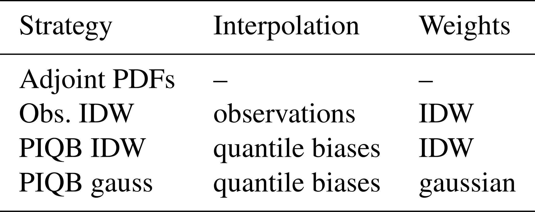
To summarize the strategies considered and cross-validated in this study, all of them are briefly described in Table 1. Please note that Adjoint PDFs does not consider any interpolation, as it functions on correcting the PDF in the entire domain as a whole. Let us further remind the reader that the cross-validation itself quantifies and compares the performance of each strategy to extrapolate data outside of the station sites through the minimal value of mean residual H_D.

Lastly, besides H_D, we shall further evaluate the performance of each strategy at station sites using several validation statistics. We shall quantify the model bias by normalized mean bias (NMB; Im et al., 2015) which describes the position of the modeled PDF relative to the observed PDF. Then, the mismatch in variability shall be quantified by a simple ratio of the modeled and observed standard deviation ${\mathit{\sigma }}_{\mathrm{M}}/{\mathit{\sigma }}_{\mathrm{O}}$. Similarly, the slope of the linear regression through the scatterplot of modeled and observed data (Slope; Karlický et al., 2017) describes the mismatch in variability with higher sensitivity to outliers, most useful for the validation of policy-relevant metrics. Finally, to compare the spatio-temporal correlation, the Pearson correlation coefficient is used. Even though the temporal component of correlation does not represent a highly relevant measure for chemistry-climate simulations, we are displaying the correlation for completeness of our analysis to demonstrate the role of spatial correlation and for consistency with previous studies (Mar et al., 2016; Karlický et al., 2017, 2024).

Table 1 The list of the four different bias correction strategies evaluated in this study highlighting the differences in interpolated quantities and weighting functions.

We shall also use the Pearson correlation coefficient to evaluate the preservation of spatial model structures after correction. This shall serve as a comparison of positive and negative anomalies from the large-scale variability of the MDA8 fields in chosen quantiles. As it cannot be simply assumed that the large-scale variability is simulated perfectly, the correlation shall be calculated using the data as they are (with a potentially dominant influence of the large-scale variability on the correlation value) as well as anomalies from the domain-wide first approximation of the MDA8 gradient in chosen quantiles (comparing the preservation of the simulated regional differences). The gradient is estimated using a multi-linear regression model with predictors of zonal and meridional indices of the domain grid-boxes, and the anomalies are generated by simply subtracting the fitted regression models from the data for each corresponding strategy (and the original simulations) separately.

3 Results and discussion

Let us now proceed to the evaluation of the performance of the CTMs, the optimization of the parameter β in Eq. (1) and α in Eq. (7) and finally the validation of the postprocessed simulations using different strategies. The validation was performed in terms of climatological seasons and focused on the qualitative shapes of the PDFs and modeled variability. As mentioned before, the analysis was performed on MDA8 of ozone, which were obtained from hourly data.

3.1 Validation of original simulations

Prior to postprocessing, a brief validation of the original simulations follows. Figure 3 shows 4 validation statistics for the original simulations performed with models WRF-Chem and CAMx. The validation shows a strong seasonal dependency of NMB for both models with higher NMB in DJF and SON and lower NMB in MAM and JJA.

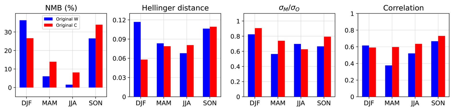
Figure 3 Seasonal validation of the original simulations using WRF-Chem (W; blue) and CAMx (C; red) against station data, from left to right: normalized mean bias (NMB), Hellinger distance, ratio of standard deviations of modeled and observed data respectively (${\mathit{\sigma }}_{\mathrm{M}}/{\mathit{\sigma }}_{\mathrm{O}}$) and Pearson correlation.

Consistently with Revell et al. (2018), the global chemistry model SOCOL overestimates tropospheric ozone concentrations in our latitudes, which may then translate into the nested domain, as reported by Karlický et al. (2024). This means that the model bias in this case most probably originates from the BCs. As stated before, ozone bias is a common problem even in other studies (e.g., Grell et al., 2005; Racherla and Adams, 2008; Mar et al., 2016; Karlický et al., 2017, 2024) and cannot be simply prevented in CTMs.

The variability of the modeled data is weaker in all seasons when compared to the observations, as seen in ${\mathit{\sigma }}_{\mathrm{M}}/{\mathit{\sigma }}_{\mathrm{O}}$. This shows that simple bias removal may not fully correct all the shortcomings of the modeled data. Consequently, despite being theoretically bound by 1, the Hellinger distance of 0.06–0.12 is still relatively high given that the simulations are supposed to approximate the atmospheric processes in a detailed way. The origin of its values can be partially seen in both NMB by shifting the modeled PDFs and the weaker variability by underestimating the widths of the PDFs, resulting in poor overlap of the modeled and observed PDFs. Additionally, the mismatch in higher moments of the PDFs may contribute as well, but they are not quantified here.

Finally, the correlation of modeled data and observations varies more notably for WRF-Chem than for CAMx, but is overall similar for both simulations. Correlation of ozone concentrations within 0.4–0.7 is well expected for CTMs of such resolutions (Grell et al., 2005; Mar et al., 2016; Karlický et al., 2017, 2024). A more detailed validation can be found in the original work of Karlický et al. (2024).

3.2 Calibration of free parameters and cross-validation

After confirming the presence of systematic errors, we proceeded with the cross-validation of each of the bias correction strategies considered using the methodology explained above. This was done to obtain the optimal values for the parameters β and α in Eqs. (1) and (7) respectively, but also to evaluate the ability of the strategies to reconstruct pseudo-observed PDFs at station sites which were omitted during calibration.

The empirical functions of the mean residual H_D were constructed with a step of $\mathrm{0.25}\times {\mathrm{10}}^{-\mathrm{3}}$ of the interpolation parameter for the range between 0.25–$\mathrm{20}\times {\mathrm{10}}^{-\mathrm{3}}$. The minima of functions corresponding to the strategies were found in each month by fitting nearby data points with a 3rd-degree polynomial and finding its minimum. Results for each of the strategies and for both simulations are shown in Fig. 4. Few important observations can instantly be made, beginning with the fact that all empirical functions are truly smooth and continuous as has been assumed, with the interpolating strategies having always exactly one minimum. The optimal values of the interpolation parameter for the gaussian weights were chosen as marked in Fig. 4. For the strategies PIQB IDW and Obs. IDW, the parameter β was optimized in the same way, but is not displayed in Fig. 4 to preserve comprehensiveness. The parameter β was ranging between 1–$\mathrm{1.5}\times {\mathrm{10}}^{-\mathrm{3}}$.

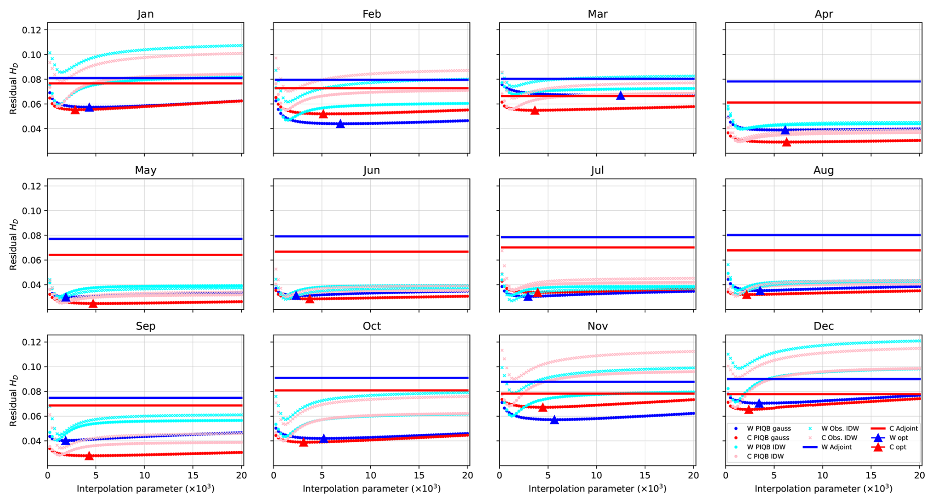
Figure 4 Empirical monthly functions of mean residual Hellinger distance H_D between the observed PDFs and their statistical reconstructions for each cross-validated station site, both WRF-Chem (W; blue) and CAMx (C; red) simulations and each of the 4 strategies: PIQB gauss (dark dots), PIQB IDW (light dots), Obs. IDW (light crosses) and Adjoint PDFs (dark lines). The optimal values of the parameter α for PIQB gauss are marked by triangles.

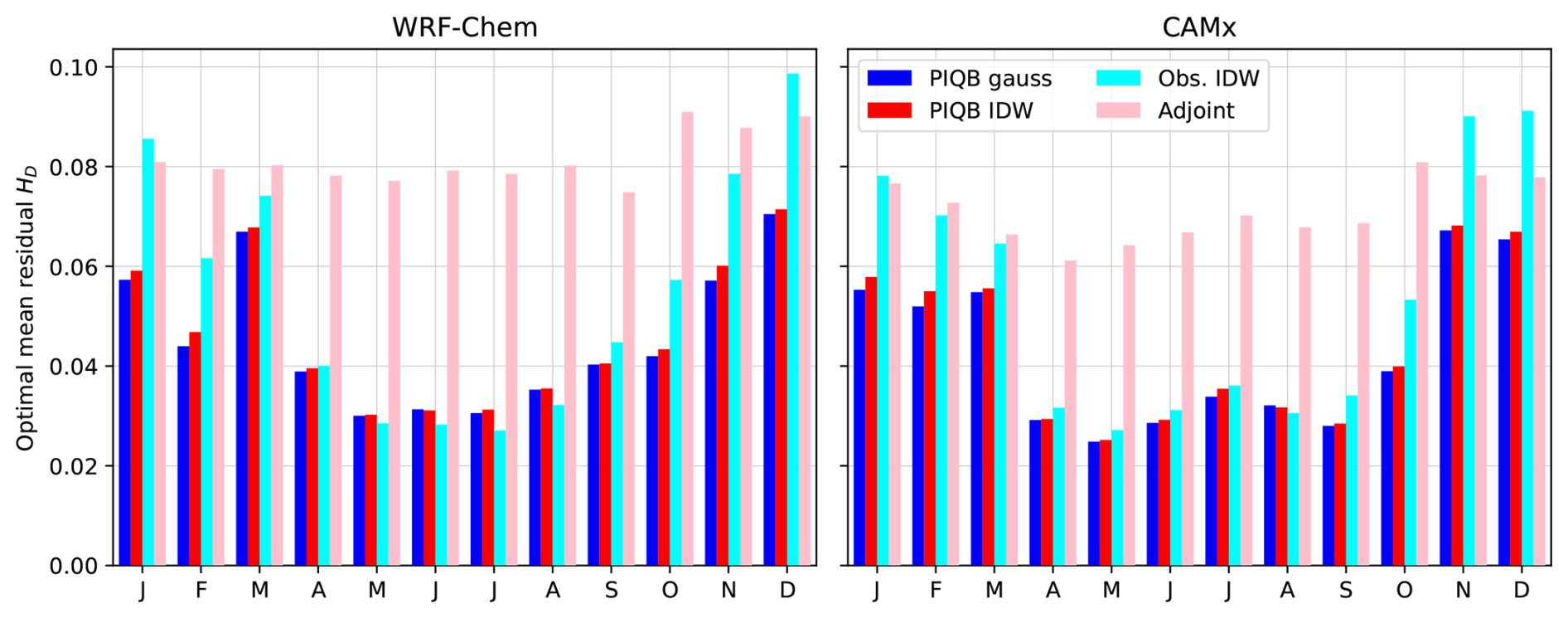
Another interesting remark is better visible in Fig. 5 where the optimal residual H_D is displayed for each month. H_D of optimized interpolating strategies exhibit an annual cycle with lower values in the warmer part of the year and the opposite in the colder part, while H_D of Adjoint PDFs does not. In this sense, it is not surprising that Adjoint PDFs performs the worst out of all of the four considered strategies with a weak annual cycle throughout the year, except for some cases in the winter period, as it forcefully increases the variability of the modeled data in the whole domain regardless of their spatial variability, which yields similar residual errors in each month. Furthermore, larger differences between interpolating strategies can be seen in the colder part of the year, while the opposite is true for the warmer part. This is because ozone concentrations correspond less to orography in summer than in winter, not only making corresponding quantities easier to interpolate, but also highlighting the importance of orographic features for a successful interpolation. All these remarks conclude that the spatial variability of the model errors plays a crucial role for bias correction. This is an important result to consider, because it shows the ability of PIQB to reliably reconstruct station PDFs at places with no stations.

Figure 5 Mean residual Hellinger distance in the empirical minima in Fig. 4 in each month for both the WRF-Chem (W; left) and CAMx (C; right) simulations and for each considered strategy, i.e., PIQB gauss (blue), PIQB IDW (red), Obs. IDW (cyan) and Adjoint PDFs (pink).

3.3 Performance of postprocessed simulations

Let us now shift our attention to the performance of the bias correction strategies listed in Table 1 using the optimal parameters for their calibration. In this section, we shall first quantitatively address the improvements to the validation statistics displayed in Fig. 3, then the preserved and resolved spatial variability of ozone MDA8 by each strategy, and lastly the ability of the strategies to capture the correct number of immission limit exceedances.

3.3.1 Statistical validation on station data

A basic seasonal validation against the data at all 165 stations is depicted in Fig. 6, as an analogy to Fig. 3 (note the different scales for NMB and Hellinger distance). Each of the bias correction strategies managed to improve NMB, Hellinger distance, the ratio of the standard deviations and correlations with measurements in each season for both simulations. The values of NMB decreased from the range of 1.5 %–36 % to −1.9 %–2.2 % and its seasonal dependency changed as well. Additionally, H_D decreased in terms of orders from 6–$\mathrm{11}\times {\mathrm{10}}^{-\mathrm{2}}$ to 2–$\mathrm{32}\times {\mathrm{10}}^{-\mathrm{4}}$, owing to the mechanism of QM which well approximates the observed PDFs. Regarding correlation with observations, it increased mostly due to the changes in spatial distributions, but also slightly due to changes in the annual cycle owing to the following mechanism.

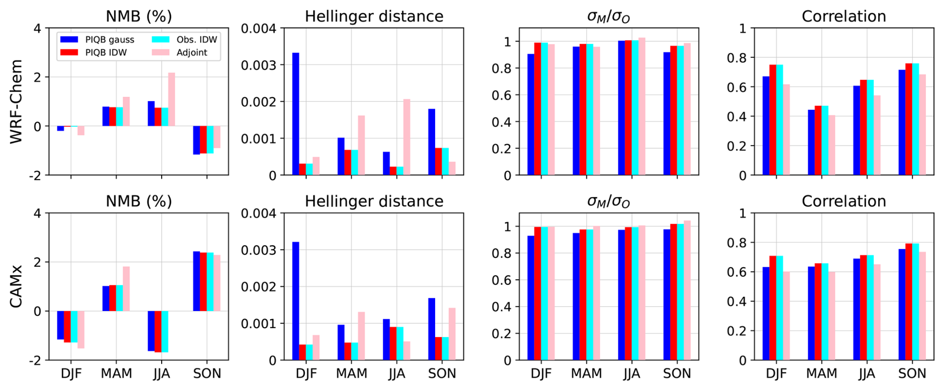
Figure 6 Seasonal validation of the postprocessed simulations using optimized strategies of bias correction against all station data: PIQB with gaussian (blue) and IDW (red) weights, Obs. IDW (cyan) and Adjoint PDFs (pink). Top row shows experiments performed on the WRF-Chem simulation, bottom row on CAMx. When comparing to Fig. 3, note the differences in scales for NMB and Hellinger distance.

As the corrections were done on 3-month long moving seasons, the corrected correlation within this seasonal scope could be either slightly increased or moderately decreased depending on the specific part of the annual cycle, as sometimes the main driver of seasonal variability corresponds to the differences between the months within the season. Further in the process, the middle month was cropped from the moving season, thus removing the relevance of the variability of individual seasons. When compared to the observations in this stage, the correlation in the monthly scope at least partly moved back in the direction of its original value before postprocessing, i.e., overall a slight increase. Lastly, when the annual cycle was re-assembled from the cropped corrected months, the seasonal correlations as depicted in Fig. 6 increased slightly due to shifts of the monthly mean values (i.e., better resolved annual cycle which then again becomes the main driver of seasonal variability). This slight increase is visible in the improvement of correlation in the case of Adjoint PDFs compared to the original simulations, because, as shall be discussed further, this strategy does not improve the spatial variability. Therefore, the improvement in the spatial correlation is generally more prominent, as seen in Obs. IDW and PIQB IDW representing strategies using an exact interpolator.

To address the qualitative comparison of the performance of each strategy, both strategies using IDW return the same validation statistic in each sub-figure of Fig. 6 despite using a different interpolation formula. This is because IDW is an exact interpolator and so the residual errors for both PIQB IDW and Obs. IDW could be practically perceived as the residual errors of QM. Therefore, if a strategy performs better than those using IDW, it is out of sheer luck. The reason for the errors to be non-zero, e.g., in the case of NMB, is once again the way the simulations were corrected – using the neighboring months as well for calibration, but only the middle month in the result to prevent overfitting. This limitation is a shared feature for each strategy.

While the validation results for PIQB IDW and Obs. IDW in Fig. 6 are theoretically indifferent to the choice of the optimal interpolation parameter, the opposite is true for PIQB gauss because it does not use an exact interpolator. It removes NMB comparably to the strategies using IDW with a slightly worse performance and similarly it still underestimates ${\mathit{\sigma }}_{\mathrm{M}}/{\mathit{\sigma }}_{\mathrm{O}}$. The residual errors of PIQB gauss have a similar seasonal dependency as PIQB IDW and Obs. IDW, suggesting that a portion of the residual errors may stem from the interpolation itself.

The strategy Adjoint PDFs is the only strategy not using interpolation, and so its seasonal dependency is different as well. This is only logical, as the error could potentially be random, because modeled and observed data from the whole domain are considered within the correction at each station and all with the same weight. This is also seen on the correlation as the differences between the increased correlation for each strategy are mainly due to different approaches to address spatial variability, and so in this sense Adjoint PDFs did not improve the correlation almost at all. Still, it performs relatively well in terms of NMB and ${\mathit{\sigma }}_{\mathrm{M}}/{\mathit{\sigma }}_{\mathrm{O}}$ compared to the other strategies.

To compare the strategies further, seemingly contradictory to the conclusions drawn from Fig. 5, PIQB gauss leaves relatively high residual errors compared to the other strategies. Naturally, this is because it does not use an exact interpolator and Fig. 6 does not provide any information about the performance outside of the station sites. In other words, Fig. 6 (showing the residual errors at places with stations) displays fundamentally different measures than Fig. 5 (showing the performances outside the station sites). Nevertheless, the errors of PIQB gauss in terms of H_D are still comparable or even lower in Fig. 6 than in Fig. 5, but the decisive figure for the performance of utilization the information from station data should be Fig. 5.

As the correction was made per months, we can compare the discrepancies of the original and corrected model data from the observations in terms of the annual cycle of MDA8. Figure A1 in the Appendix shows the annual cycles of the observations and the original simulations as well as their corrections. After the correction, all strategies perform very similarly, reducing the bias and increasing the monthly variability, thus adjusting the annual amplitudes as well. It is interesting to note that the qualitative shapes of the annual cycles did not change for either of the simulations. This can be observed on the fact that throughout all bias correction strategies, the corrected CAMx simulation still exhibits residual bias most notable in April and August, while the WRF-Chem simulation retained a sharp increase of MDA8 from February to March as well as a subtle increase from March to April. These residual errors are slight and very practical. They once again prove that the statistical procedures do not overfit, therefore suggesting a possibility to use them for correcting climate projections while retaining the qualitative character of the modeled data.

Figure A1 also visualizes the main flaws in the original simulations, which helps to understand the key relationships between the validation statistics displayed in Figs. 3 and 6. Both simulations exhibit a systematic bias in the annual cycle, as well as shortage of monthly variability (i.e., the lengths of error bars). And so joining both types of discrepancies into a common problem in the shapes of the PDFs leads us to the motivation behind minimizing H_D in the calibration phase of the bias correction.

3.3.2 Spatial distributions of MDA8

To fully understand the differences between the considered strategies of bias correction outside the station sites, one must look at the resolved spatial distributions after correction by each of them. Figure 7 shows the spatial distribution of mean summer-time MDA8 in the WRF-Chem simulation before and after correction with marked stations, while Fig. 8 shows the same for the CAMx simulation.

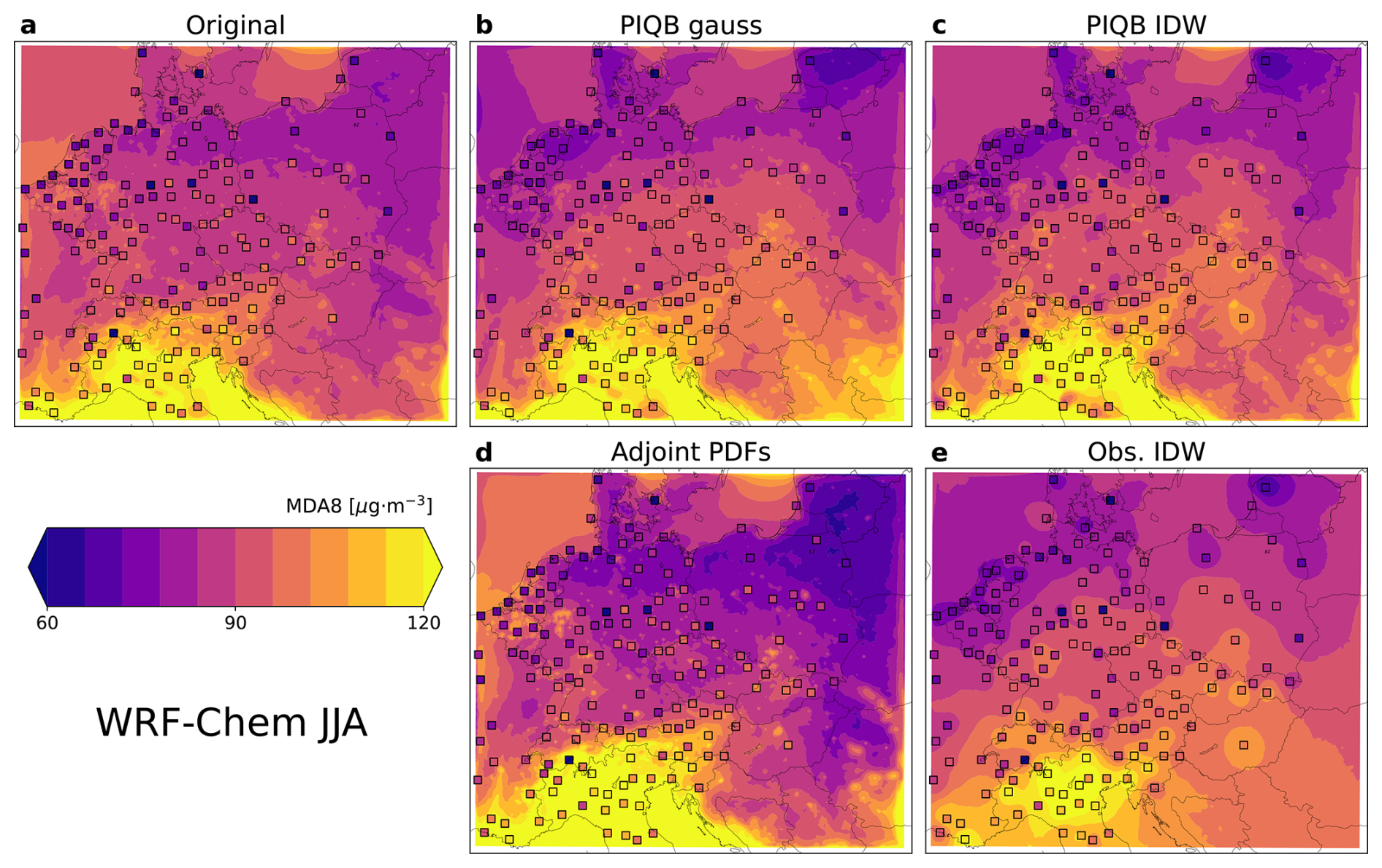
Figure 7 Mean summer-time ozone MDA8 in the model domain as simulated by the WRF-Chem simulation (a) and their corresponding corrections using the strategies of PIQB gauss (b), PIQB IDW (c), Adjoint PDFs (d) and Obs. IDW (e). Colored squares mark measured values.

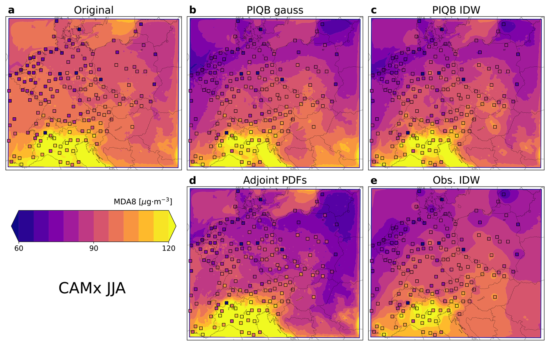
Figure 8 Same as Fig. 7, but for the CAMx simulation.

The following claims apply to both simulations and their conclusions are apparent in both Figs. 7 and 8. The original simulations do not take into account for the real observed spatial variability, showing a relatively similar meridional gradient of mean MDA8, but exactly opposite zonal gradient than the observations. Once the strategy of Adjoint PDFs is applied, this difference in gradients only becomes highlighted. That is because the Adjoint PDFs is only calibrated on the validation displayed in Fig. 3, i.e., the calibration tries to increase the variability of the model data to fit the observations, which results in a stronger, yet still incorrect, zonal gradient.

In the case of the strategy Obs. IDW, it results in fitting the observations almost perfectly, since IDW is an exact interpolator. Therefore, the zonal gradient fits better than in the case of Adjoint PDFs, showing the lowest MDA8 in the north-west corner of the domain instead of the north-east. Such a phenomenon is better visible in Figs. A2 and A3 on the median bias where Adjoint PDFs shows a gradient in the direction from the south-west to north-east, while Obs. IDW (which shows a comparison with the actual station data) exhibits a gradient from the south-east to the north-west of the domain. However, this strategy smooths out the mean MDA8 field completely, omitting for the spatial variability described by the model, most notably seen in the south-east corner of the domain with a limited number of stations. Please note that the plots of Obs. IDW in Figs. 7e and 8e look different for both simulations, despite both describing the result of interpolating measurements. That is because after the interpolation of station data (using different parameters), QM was applied. Therefore, the differences between these two figures can be attributed to the differences between the interpolation parameters β, the differences between the model simulations and the precision limits of QM.

Moving on to the interpolation of quantile biases, PIQB IDW not only corrects the zonal gradient of mean MDA8 in both Figs. 7c and 8c, but also preserves the qualitative spatial variability as modeled by the WRF-Chem and CAMx simulations, which is one of the characteristics of PIQB in general. To compare it with Obs. IDW, despite having the same residual errors in Fig. 6 and fairly similar quantile bias fields in Figs. A2 and A3, they perform very differently in terms of cross-validation in Fig. 5, which is apparent in the spatial distributions of mean MDA8 in Figs. 7 and 8 as well. The key differences between PIQB IDW and Obs. IDW are better visible in cases where the spatial distribution of mean MDA8 is less smooth, e.g., winter periods in Figs. A4 and A5, where considering the modeled spatial variability results in resolved orographical effects, such as higher concentrations in the Carpathian mountains. This also demonstrates why the residual cross-validation errors in Fig. 5 are much higher in the winter period for Obs. IDW compared to PIQB IDW or PIQB gauss.

The last strategy is PIQB gauss in Figs. 7b and 8b, which uses the same interpolation formula as PIQB IDW, i.e., interpolation of quantile biases, but a smoother weighting function, which smooths the quantile bias fields in Figs. A2 and A3. As a result, a sacrifice was made in terms of not fitting the observations perfectly, as seen in Fig. 6. In the JJA case, the mean interpolation error in the whole domain for PIQB gauss in terms of Hellinger distance within cross-validation is not reliably the lowest of the four considered strategies, but is comparable (and consistently lower in other months) to those of Obs. IDW and PIQB IDW. This is because not using an exact interpolator in this case preserves more of the model structure, which is important for orographic effects more notable in the colder parts of the year seen by the models.

To support the claims on the unresolved and added spatial variability of each strategy, Fig. 9 shows the spatial correlations of MDA8 fields in chosen quantiles (5, 50 and 95) in the simulations postprocessed by each considered strategy with the original simulations. The correlation was calculated using the raw data and the anomalies with respect to a regression model considering predictors of zonal and meridional indices of domain grid-boxes, as explained in the methodology section. Generally, the spatial correlations are relatively high, as they were calculated using the data in the whole domain, meaning that they also include the differences between land and ocean, etc. Regarding individual strategies, the correlation of the original simulation with Adjoint PDFs is essentially almost equal to 1, because it does not change the simulated spatial variability at all, as previously discussed and shown in Fig. 6. Its counterpart Obs. IDW correlates with the original simulations the lowest of all strategies, because it does not consider the model spatial variability during the correction. Lastly, PIQB IDW and PIQB gauss represent a compromise of the two strategies, showing a relatively high correlation with the original simulations, but with a generally slight setback, suggesting that PIQB changes the spatial variability at least a little.

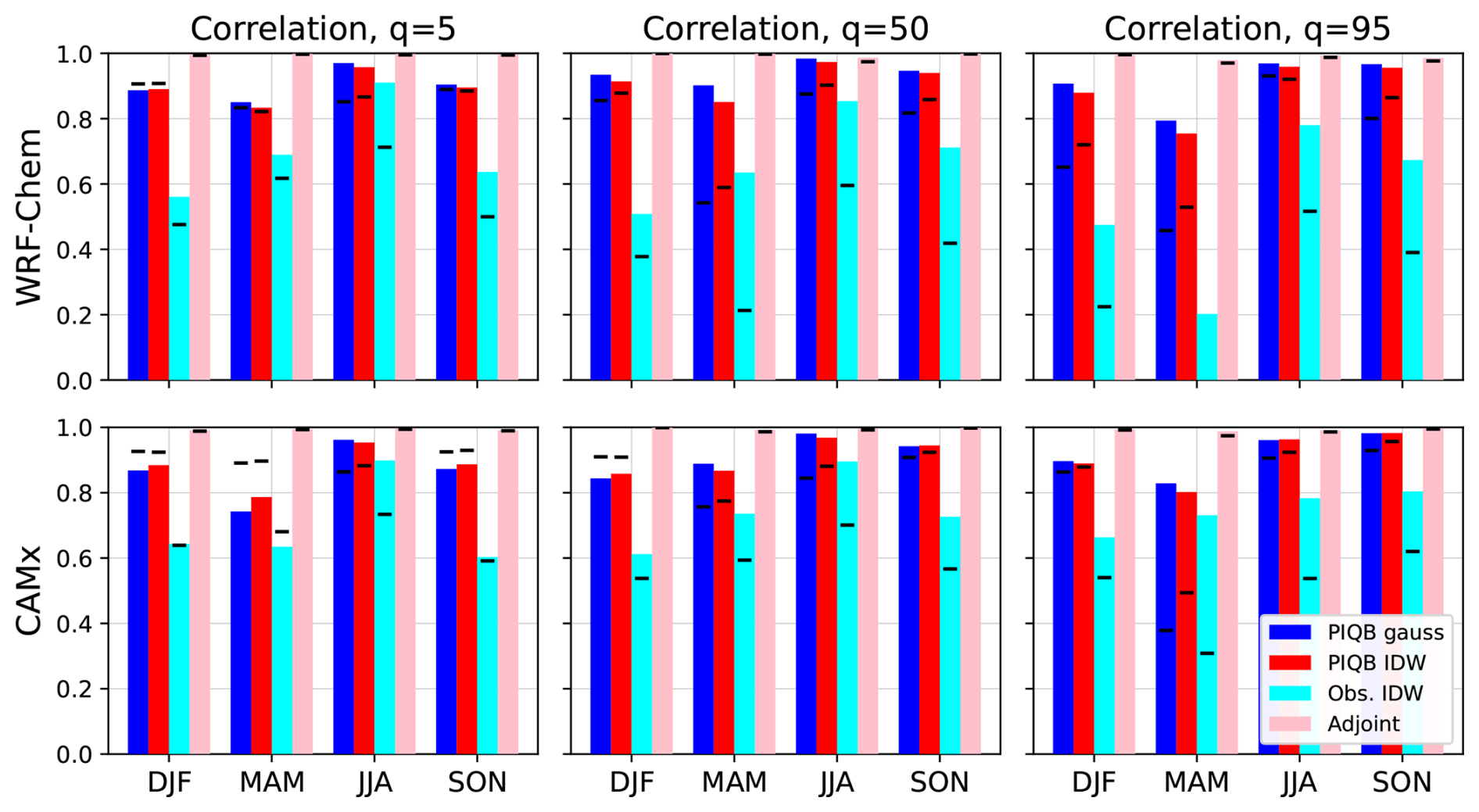
Figure 9 Seasonal spatial correlations of the original simulations using WRF-Chem (top row) and CAMx (bottom row) with their postprocessed products using strategies of PIQB gauss (blue), PIQB IDW (red), Obs. IDW (cyan) and Adjoint PDFs (pink) in terms of grid-box-wise quantiles of MDA8 of 5 (left), 50 (center) and 95 (right). The correlations of the raw data are marked by black dashes while the correlations plotted as bars were calculated using anomalies from regression models of each dataset considering predictors of indices of domain grid-boxes (representing the domain-wide large-scale gradient of MDA8). In MAM in the WRF-Chem simulation for q=95 the raw correlation of Obs. IDW with the original simulation was approximately −0.2 and is therefore not seen in the figure.

In order to differentiate between correlation originating from the fine model structures and large-scale gradients, we may focus on the differences between the bars and dashes in Fig. 9. The generally lower correlation of the raw data shows the inability of the original simulations to provide the actual large-scale variability measured by the stations, as is also seen in the gradients of quantile bias fields in Figs. A2 and A3. On the other hand, removing the large-scale gradient results most of the time in an increase of correlation of quantiles 50 and 95 for each interpolating strategy, which means that the regional relative differences are being simulated relatively well. Both PIQB gauss and PIQB IDW show higher spatial correlations than Obs. IDW because they retain more of the modeled fine structures, as demonstrated in Figs. 7 and 8, resulting in a greater match in the regional differences both before and after the subtraction of the large-scale variability. Furthermore, one may notice that the correlations of PIQB gauss are in most cases greater than those of PIQB IDW, suggesting that the gaussian weighting functions preserve more of the model structures, but such differences are generally negligible compared to the difference from Obs. IDW.

3.3.3 Immission limit exceedances

A general feature among the correction strategies is the correction of model variability and spatial distributions, which is relevant for the spatial distribution of policy-relevant metrics as well. Figure 10 shows the mean annual number of days with MDA8 exceeding 120 µg m⁻³ in the WRF-Chem simulation before and after correction, while Fig. 11 shows the same for the CAMx simulation. The immission limit of ozone does not allow for the annual number of such days to be higher than 25 on average in 3 consecutive years (EUR-Lex, 2015). As we are presenting climate simulations, this average was taken in the whole 10-year-long period for both the station and model data and the threshold exceedance is marked red.

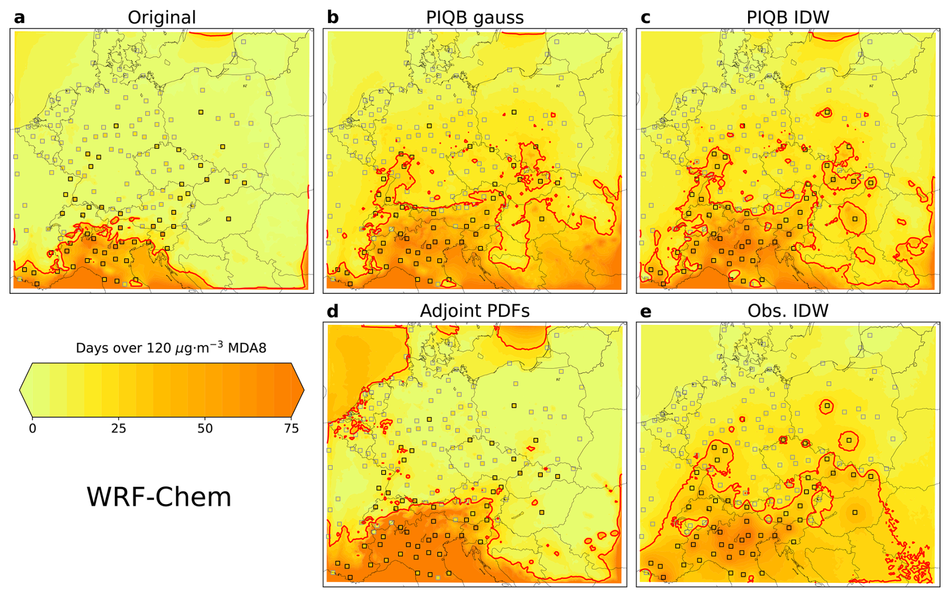
Figure 10 Mean annual number of days above 120 µg m⁻³ MDA8 of ozone on average in 2007–2016 in the WRF-Chem simulation before (a) and after correction using the strategies of PIQB gauss (b), PIQB IDW (c), Adjoint PDFs (d) and Obs. IDW (e). The station sites are marked by gray squares, those with immission limit exceedance defined by the threshold of 25 d, which took place at 53 station sites, are marked black, red contour marks the threshold as predicted by the model data.

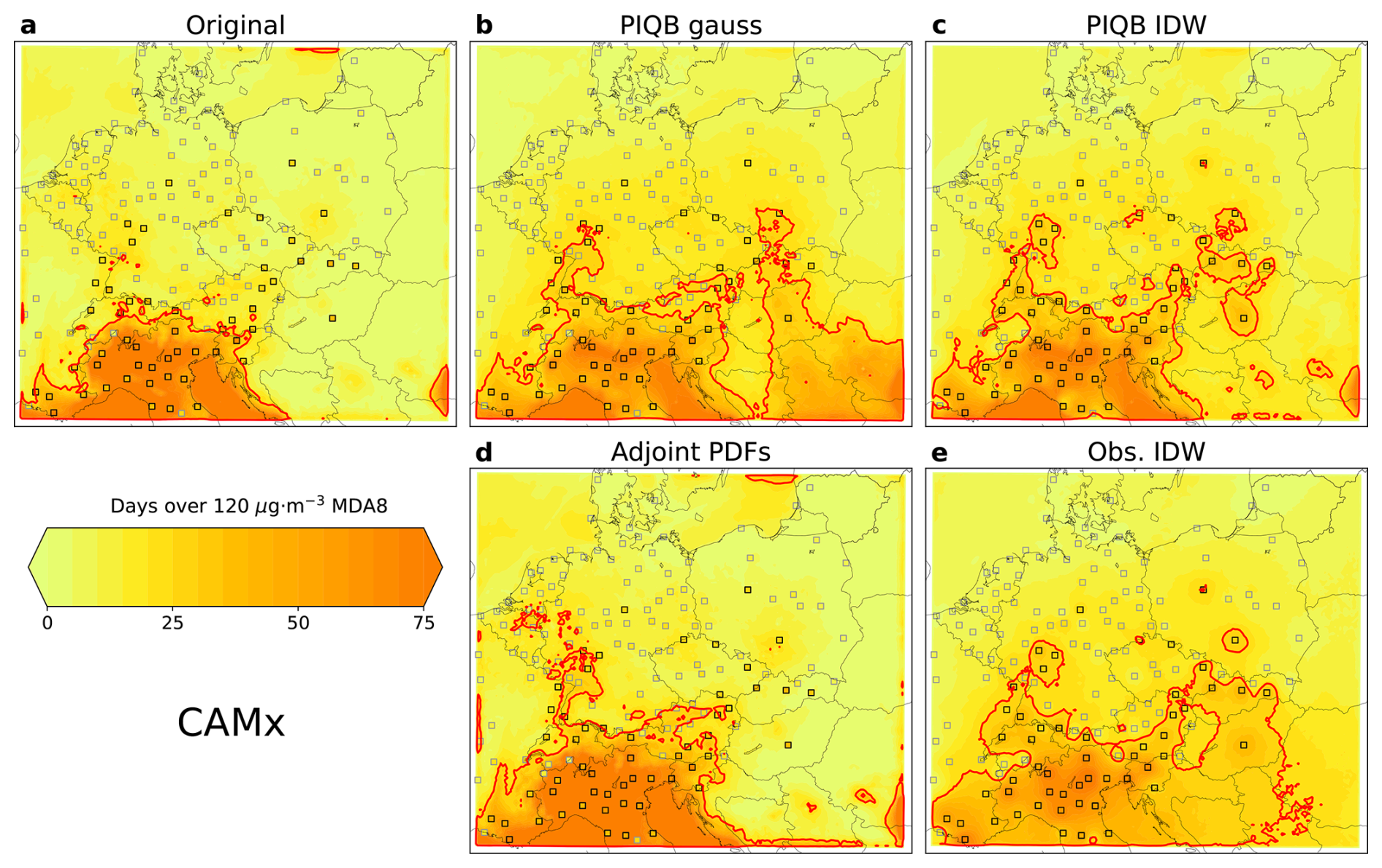
Figure 11 Same as Fig. 10, but for the CAMx simulation.

In both model cases in Figs. 10a and 11a, it is apparent that the original simulations have very limited variabilities and the area of exceeded immission limit spans only to the north of Italy, while in the case of observations, many of the stations with exceedances are located also further north and east in the center of the domain. Upon correcting the simulations using Adjoint PDFs, this area spreads further, mostly to the north and west, resulting in some exceedances even in Austria and Germany. In the case of the WRF-Chem simulation in Fig. 10d, Adjoint PDFs hints exceedances even over sea in the north-west corner of the domain, showing how this strategy does not consider the spatial distribution of observations, but only increases the variability of the model data in the whole domain.

In the case of Obs. IDW, the red contour in Figs. 10e and 11e spreads further and envelops the stations with exceedances almost perfectly. However, there are some stations in Poland and Germany which cannot be attributed to this spread directly, despite being enveloped by the contour as well. This is the result of overfitting the correction with station data, disregarding the modeled spatial variability.

This shortcoming is partly solved by switching to a different interpolation formula, i.e., to PIQB IDW. The contoured borders in Figs. 10c and 11c look more natural and it is apparent that the number of days have sharper gradients within the contoured area, hinting a better use of the model spatial variability during the correction. Nevertheless, there are some singular contoured points in the eastern part of the domain which cannot be linked directly to the southern area of exceedance.

Lastly, PIQB gauss solves this problem, connecting the singular points without overfitting the correction with station data. In terms of the ability to qualitatively resolve the spatial distribution of the immission limit exceedances, PIQB gauss shows the most plausible results for both simulations. The key difference between PIQB gauss and PIQB IDW is in the south-eastern part of the domain with a limited number of stations, where the gaussian interpolation assumes generally more days above the threshold than IDW.

To quantify the differences in the number of days exceeding the immission limit, one may treat this quantity as a variable which can be validated. Such a validation is displayed in Fig. 12 for both before and after correction. As is apparent, all strategies mitigate the bias in the number of days of exceedance, except for Adjoint PDFs in the CAMx simulation, showing how the unrealistically high mean concentrations over northern Italy in the original simulation transformed into the overestimation of exceedances in the rest of domain after correction. Furthermore, Adjoint PDFs in particular is also the only strategy resulting in an increase of B₅₀ in northern Italy as seen in Figs. A2 and A3, consequently overshooting of the total immission limit exceedances and their variability, as discussed further. On the other hand, contrary to Figs. 3 and 6, the correlations in Fig. 12 (spatial correlations) are expectedly increased by all considered strategies, most notably by both Obs. IDW and PIQB IDW as they use an exact interpolator.

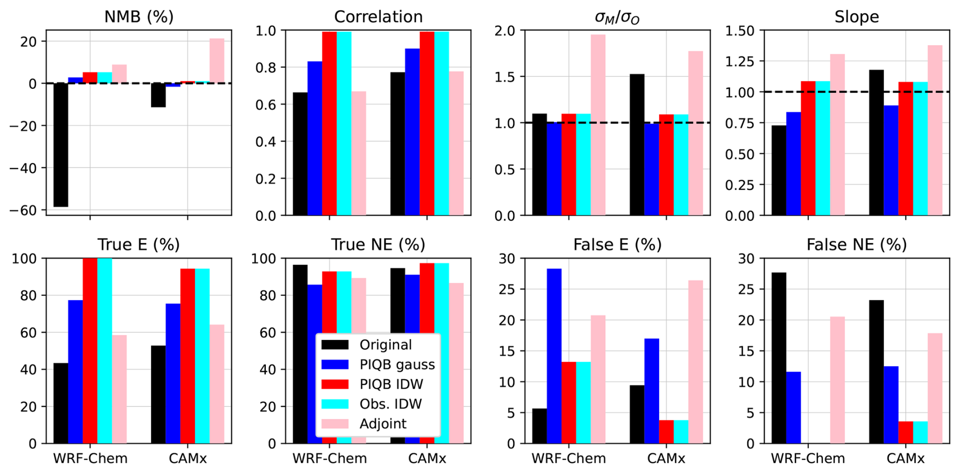
Figure 12 Validation of number of days above the 120 µg m⁻³ threshold (upper panel) using NMB, Pearson correlation, ${\mathit{\sigma }}_{\mathrm{M}}/{\mathit{\sigma }}_{\mathrm{O}}$ and the slope of linear regression in the scatterplot of observations and modeled values. Lower panel displays predictions of the immission limit exceedances in terms of the success rate of true/false predicted exceedance/non-exceedance (E/NE; i.e., elements of the confusion matrix). The black dashed line marks the ideal match. Note the differences in scales in the lower panel between True and False.

Regarding variability, the ratio of standard deviations ${\mathit{\sigma }}_{\mathrm{M}}/{\mathit{\sigma }}_{\mathrm{O}}$ gets closer to the perfect match of 1 in all cases except for Adjoint PDFs. The reason is that Adjoint PDFs forces the variability of MDA8 to be greater than the original model data in the whole domain, regardless of the station spatial distribution of MDA8. This results in an expansion of the threshold contour in the south of the domain in Figs. 10d and 11d while retaining relatively low values in the center of the domain, thus inflating the variability of immission limit exceedances. Discussing the variability further, the slope statistic of the original WRF-Chem and CAMx simulations have the exact opposite shortcoming relative to the perfect match of 1 and all strategies compensate it at least partially, except for Adjoint PDFs which results in its overestimation for similar reasons as in the case of ${\mathit{\sigma }}_{\mathrm{M}}/{\mathit{\sigma }}_{\mathrm{O}}$.

In the lower panel of Fig. 12, the success rates of predicting an immission limit exceedance (E) or non-exceedance (NE) are displayed, which is the percentage of the count of binary E/NE at station sites. It is clear that each strategy enhances the original results, increasing the true predicted E from 40 %–50 % to almost 60 %–100 %. On the other hand, predicting true NE is generally slightly worse after the corrections, which is complementarily seen in the overestimation of false E, i.e., mistakenly predicting an E at a station site without it. The overall predictions were better in terms of true NE and false E than in the case of true E and false NE, which could be due to the fact that the number of stations with a true E is 53 while without it is 112, and so the success rates were more sensitive to errors.

Regarding differences between correction strategies in Fig. 12, both Obs. IDW and PIQB IDW expectedly outperform all of the other strategies when validated on station data, as they use an exact interpolator. PIQB gauss in this sense performs worse than that, but still better than Adjoint PDFs in terms of predicting a true E. On the other hand, the true NE and false E seem to be more model dependent in terms of differences between strategies, showing worse performance of PIQB gauss compared to Adjoint PDFs for the WRF-Chem simulation, while the opposite is true for the CAMx simulation. This difference in particular can be attributed to the different spatial variabilities predicted by both models.

4 Conclusions

In this study, we presented a newly introduced strategy to use station data for bias correction of MDA8 of tropospheric ozone concentrations and compared its performance with other strategies applied on the outputs of two 10-year-long simulations made by the WRF-Chem and CAMx models. Our strategy involved the interpolation of station quantile biases into the regular model grid and we demonstrated its flexibility using two different weighting functions for spatial interpolation, i.e., IDW and gaussians.

First, we tested the ability of each strategy to interpolate station data using methods of cross-validation. The results showed that PIQB generally leaves the least minimal residual Hellinger distance, which demonstrates that it performs the best in terms of reconstructing the observed PDFs at places with no observations, while the overall better interpolation option for PIQB in the whole year was the gaussian interpolator.

Regarding residual errors after full correction at station sites, the errors and differences between strategies were substantially smaller compared to those resulting from cross-validation, while the best performing strategies were Obs. IDW and PIQB IDW. This was hardly surprising, as IDW is an exact interpolator and the corrected simulations were validated this way only at station sites. Since the simulations corrected by both strategies yield identical residual errors, one could come to a wrong conclusion that both strategies perform the same. To avoid such conclusions, either a cross-validation or maps of mean MDA8 must be analyzed.

The spatial distributions of MDA8 using different strategies showed that the strategy of Adjoint PDFs does not add any new information regarding spatial distribution of station data. In contrast to that, Obs. IDW resulted in a better agreement with stations, but omitted modeled features. In this sense, both PIQB IDW and PIQB gauss represented a middle ground between the two, resolving modeled features while preserving the spatial variability of station data.

Evaluating the performance of each strategy on a derived quantity, such as number of days with MDA8 above the 120 µg m⁻³ threshold, may be more convincing. Even in this case, both PIQB IDW and PIQB gauss mostly outperformed the other two strategies, i.e., Obs. IDW and Adjoint PDFs, in terms of resolving continuous contours of immission limit exceedances. In this sense, the success rate of both simulations to predict an immision limit exceedance improved after the correction by all of the strategies, but most dramatically by PIQB IDW, which preserved modeled features as well.

Ultimately, our findings show that PIQB performs satisfyingly well at a relatively high resolution, making it a suitable strategy to use station data for bias correction of chemistry-climate simulations. Results in this study thus suggest the possibility of using ground based station data to correct related systematic errors in climate projections of ozone MDA8 as well.

Appendix A

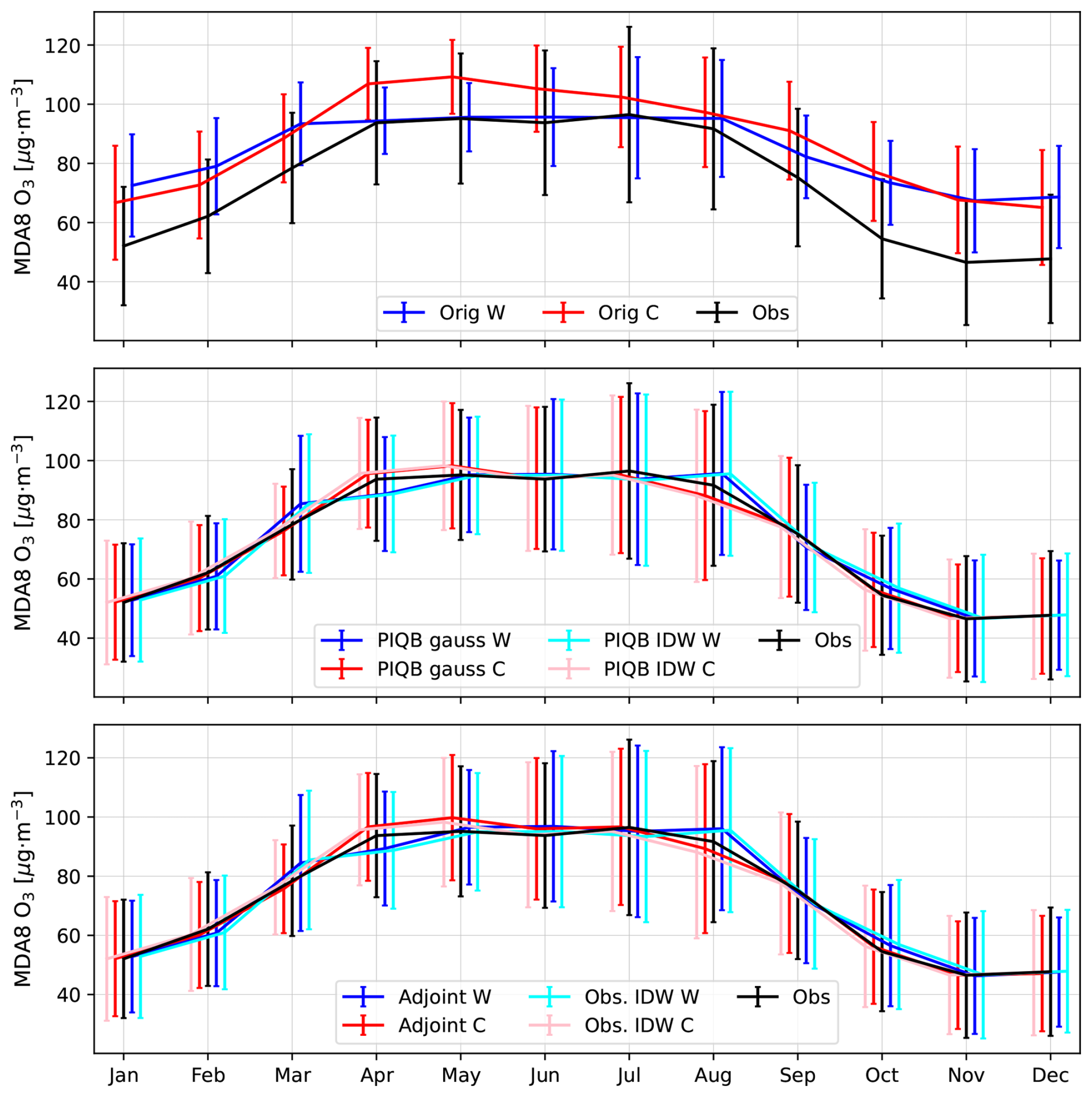
Figure A1 The mean and the standard deviations of monthly MDA8 of the observations (black) and original and processed simulations corresponding to WRF-Chem (W; blue) and CAMx (C; red). The top panel shows the original data, the middle panel shows PIQB gauss (dark) and PIQB IDW (light) and the bottom panel shows the correction by Adjoint PDFs (dark) and Obs. IDW (light).

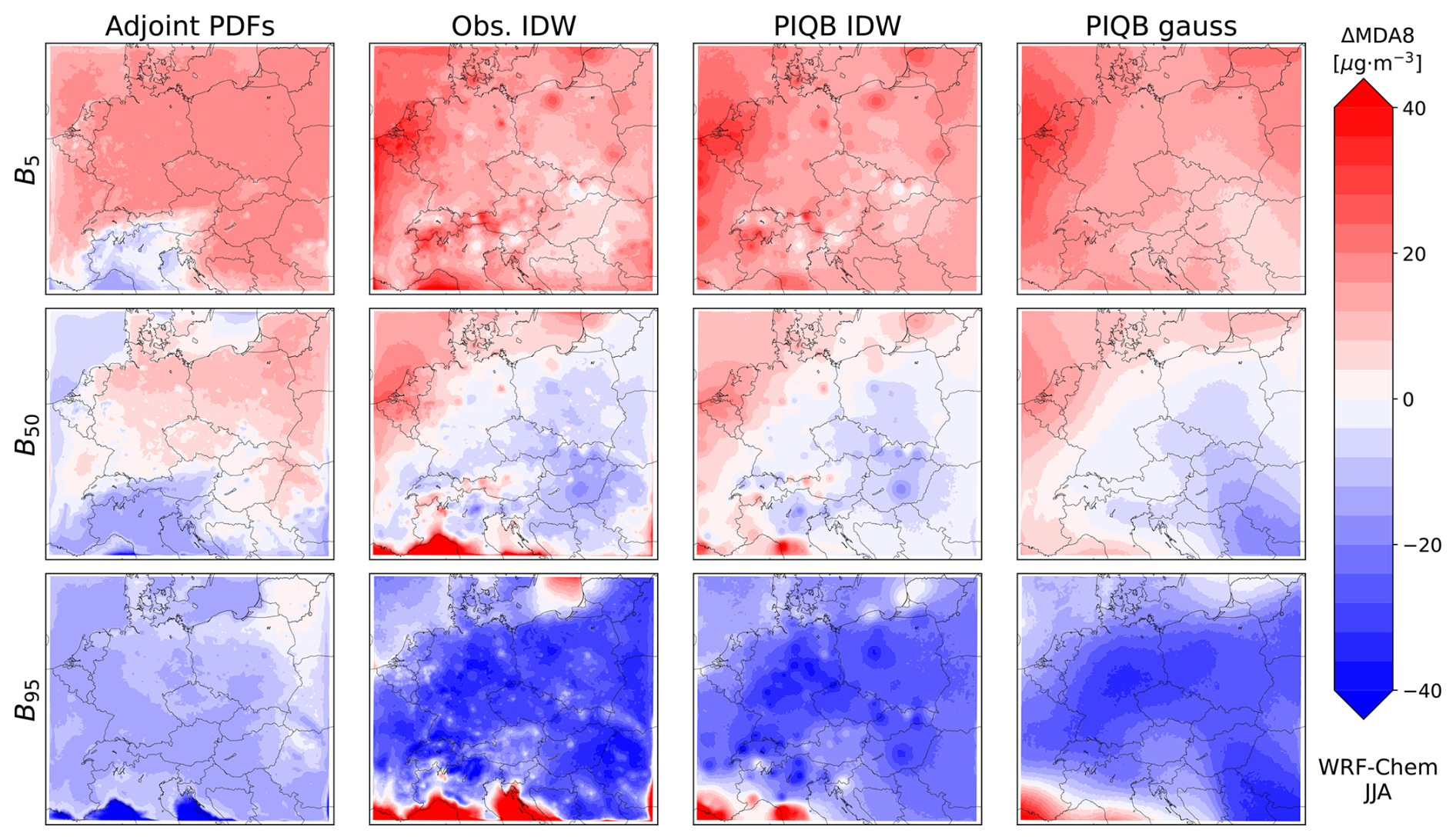
Figure A2 Summer-time quantile bias fields of MDA8 (i.e., the corrected quantiles subtracted from the original quantiles) for the WRF-Chem simulation as corrected by each considered strategy for the quantiles of 5 (top row), 50 (middle row) and 95 (bottom row). Red color marks predicted overestimation while blue color marks predicted underestimation by the corresponding strategy.

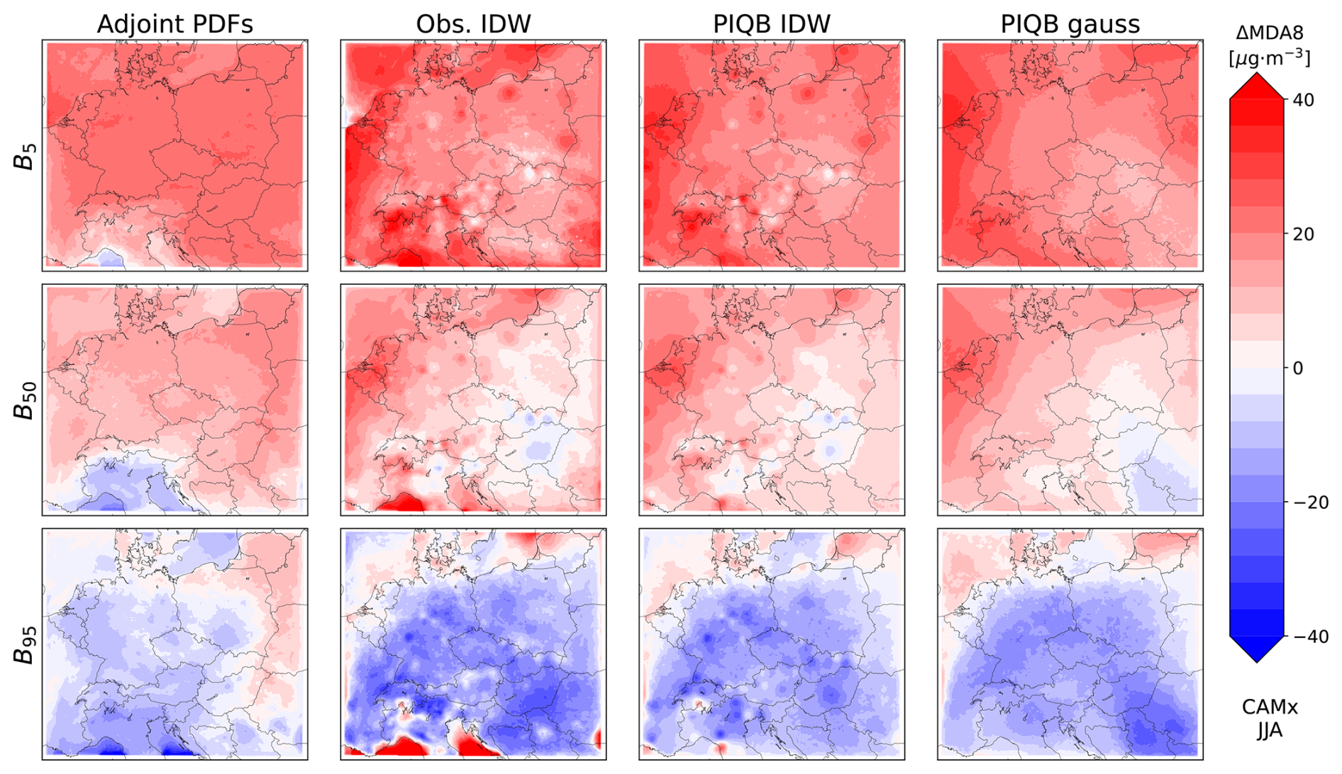
Figure A3 Same as Fig. A2, but for the CAMx simulation.

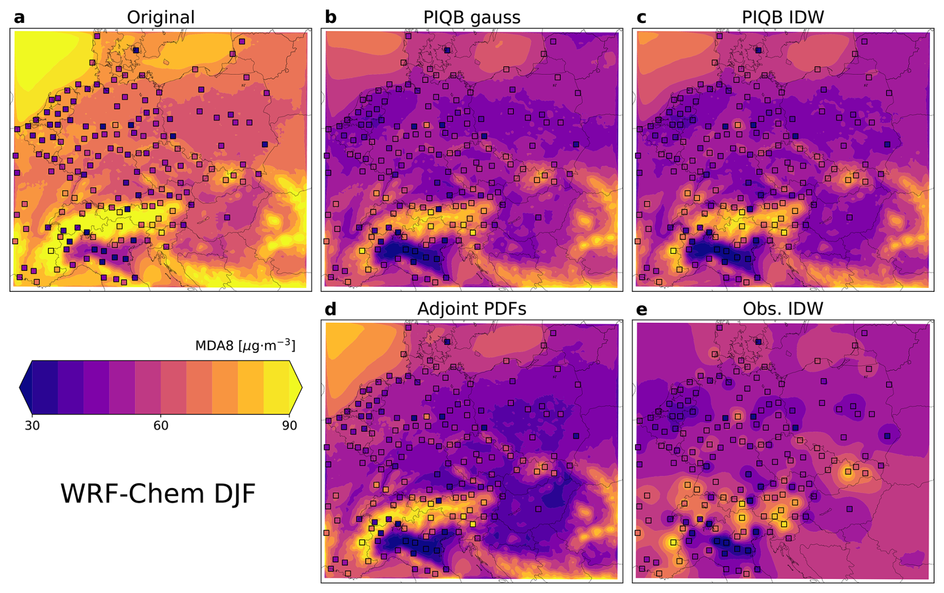
Figure A4 Mean winter-time ozone MDA8 in the model domain as simulated by the WRF-Chem simulation (a) and their corresponding corrections using the strategies of PIQB gauss (b), PIQB IDW (c), Adjoint PDFs (d) and Obs. IDW (e). Colored squares mark measured values.

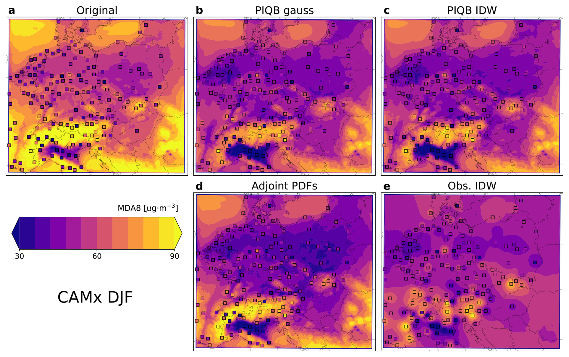
Figure A5 Same as Fig. A4, but for the CAMx simulation.