New generic coupling adapters for ice sheet and subglacial hydrology models (ISSM-preCICE Adapter 0.4, CUAS-MPI 0.1)

Adequate Earth system simulations require interactions between the atmosphere, the ocean, and the ice sheets. To this end, numerical solvers that compute the evolution of the different Earth system components are coupled. There are frameworks and libraries for coupling that handle the complex tasks of coordinating solver execution, communicating between processes, and mapping between different meshes. This allows solvers to be developed independently without compromises on numerical methods or technology. Code reuse is improved, both over large, monolithic software systems that reimplement each coupled model as well as over ad-hoc coupling scripts.

In this work, we use the preCICE coupling library to couple the Ice-sheet and Sea-level System Model (ISSM) with the subglacial hydrology model CUAS-MPI. An adapter for each model is required to pass meshes and coupled variables between the model and preCICE. We focus mainly on the technical aspects (design, development, and use of the adapters, choice of coupling library, and large-scale performance analysis), using a synthetic setup to verify functionality and correctness.

The adapters we developed are generic and reusable for use cases other than ice-hydrology coupling. Computational performance for the coupled system is measured on a high-performance computing cluster. We find that coupling with preCICE has low computational overhead and does not negatively impact scaling. A comparison between unidirectional and bidirectional coupling for the synthetic ice sheet shows that the coupling captures the anticipated feedback mechanisms between the two systems. The coupled simulations are numerically stable, despite the nonlinearities in the physical system. The generic coupling library preCICE is well suited for our use case and has advantages as well as disadvantages over Earth System Model-specific libraries.

The new framework and code enable studies of the subglacial hydrological systems of ice sheets, as well as coupling ISSM or CUAS-MPI with other codes, such as in global Earth System Models or process models.

1 Introduction

Ice sheet dynamics is a gravity-driven, lubricated flow, forced by changes at its boundaries, such as the ice-atmosphere interface, the ice–ocean interface and the conditions at the ice base. Beneath the ice sheet, a subglacial hydrological system exists that is fed by basal melting due to heat flux from the lithosphere and frictional heating. This hydrological system affects the ice sheet through changes in water pressure, while the ice sheet influences the subglacial system through changes in basal melt rates and ice sheet thickness. While the hydrological system evolves on long time scales in the center of ice sheets, at the margins, particularly in Greenland during the melt season, the evolution is accelerated considerably. Both observations (Ing et al., 2024) and modeling (de Fleurian et al., 2022) have shown the high complexity of the feedback between hydrology and ice sheet. Therefore, coupled simulations are required to study the evolution of both systems and their effect on each other. As both systems include non-linear processes, special care is required when simplifying the interactions of the system to a uniphysics problem, as also suggested by Keyes et al. (2013). This work presents a framework for simulating interactions as a multiphysics problem and applies it to an artificial setup and to Greenland.

The Ice-Sheet and Sea-level System Model (ISSM, Larour et al., 2012) is a feature-rich ice sheet model. Among its capabilities, it provides a selection of subglacial hydrology models, including the Subglacial Hydrology and Kinetic, Transient Interactions model (SHAKTI, Sommers et al., 2018), the Glacier Drainage System (GlaDS, Werder et al., 2013), and the Double-Continuum model (DoCo, de Fleurian et al., 2016). These models are fully integrated into ISSM, using the same mesh and finite-element solvers. GLaDS is also included in the ice sheet model Elmer/Ice (Gagliardini et al., 2013). Other ice sheet models, like PISM (Khrulev et al., 2025), also have their own hydrology models. While monolithic software development can be easier (e.g., a single build process and shared data structures), it also has disadvantages, including increased complexity and reduced reusability.

In this paper, we present a different, partitioned approach. Fischler et al. (2023) recently published CUAS-MPI (subsequently referred to as CUAS), a stand-alone subglacial hydrology model. ISSM and CUAS rely on different spatial and temporal discretizations, so CUAS cannot be directly integrated into ISSM. To couple the two models, we use an external independent coupling library, namely the general-purpose coupling library preCICE (Chourdakis et al., 2022). We developed adapters for both models that link them to preCICE. This approach has several advantages over directly integrating CUAS into ISSM. The models can be developed independently and make their own choices regarding discretization and numerical methods. Moreover, coupling libraries, such as preCICE, make the setup more configurable and extendable – for instance, by adding further components like an existing ocean circulation model or replacing existing components.

As a general-purpose coupling library, preCICE follows an application-agnostic coupling approach. This is in contrast to specialized Earth System Modeling (ESM) couplers, such as OASIS3-MCT (Craig et al., 2017), YAC (Hanke et al., 2016), or ESMF (ESMF Core Team, 2026). While any of these couplers could have been used in principle, using preCICE allows us to evaluate it in a context in which it has not been extensively tested yet. Specialized couplers offer coupling methods, particularly data mapping methods, which are optimized to handle 2D fields on spherical surface meshes and are, thus, well suited to model global effects on the whole Earth. preCICE, in contrast, treats meshes as clouds of scattered Cartesian points. A manuscript in review studies the viability of this approach for global models (Hocks and Uekermann, 2026). In addition, preCICE lacks conservative data mappings¹, among other specialized features. However, the missing specialization of preCICE is less important in non-global ESM scenarios, such as the setup of this paper. In addition, preCICE provides features such as implicit coupling schemes (Mehl et al., 2016, often referred to as iterative coupling in the ESM literature, e.g., in Marti et al. (2021)) and time interpolation (Rodenberg and Uekermann, 2025) that are not typically offered by ESM couplers and could provide benefits to some applications.

Beyond different feature sets, while specialization allows for more focused development, the generality of preCICE also brings the soft benefits of a potentially larger user and developer community: cross-domain knowledge transfer, more sustainable software development, and integration in widely used simulation software, e.g., OpenFOAM (Chourdakis et al., 2023) and FEniCS (Rodenberg et al., 2021), that can be used to develop new models.

Sect. 2 of this manuscript covers the software packages that are involved. First, we describe the coupling library preCICE and the existing solvers² ISSM and CUAS. Then, we present the newly developed adapters. In Sect. 3, we show the setup and results of a few basic experiments we performed to test the coupling and the computational performance. In Sect. 4, we discuss our findings and plans for future development.

2 Software

In the following, we describe all the software components necessary for the coupling of ISSM and CUAS. Figure 1 shows an overview of the coupling setup. We provide brief summaries of the three existing codes, with a focus on the technical details relevant to coupling: the preCICE coupling library, the ice-sheet model ISSM, and the subglacial hydrology model CUAS. The newly developed preCICE adapters for ISSM and CUAS are described in detail.

.

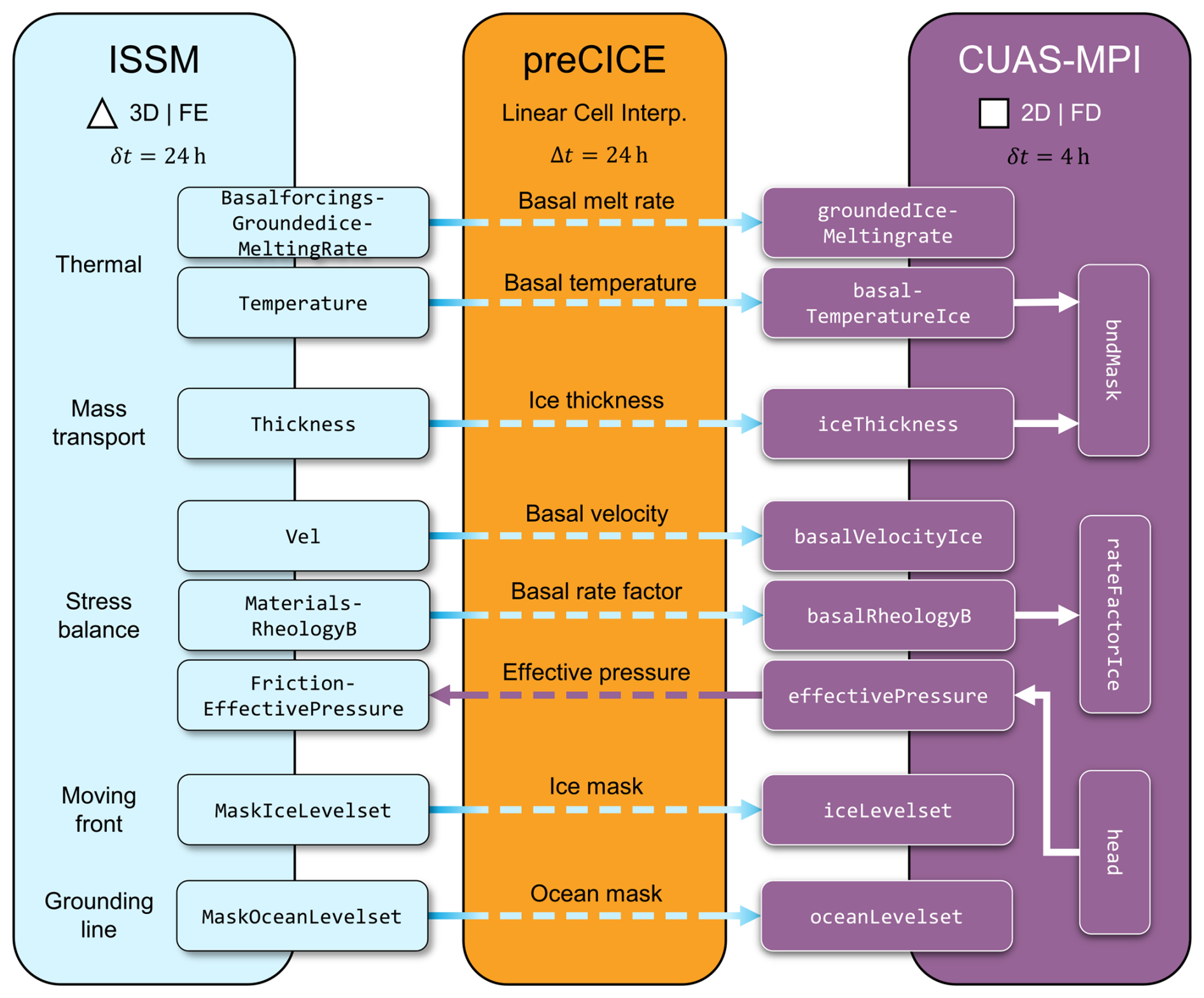
Figure 1 Overview of coupling between ISSM and CUAS-MPI. The coupling library preCICE handles communication and data mapping between the ice sheet and hydrology models. The models are free to use their own meshes (unstructured triangular or regular rectangular) and time steps. Coupled variables are listed by the name internal to the corresponding solver/adapter. ISSM uses FrictionEffectivePressure to compute sliding. CUAS uses the variables received from ISSM as a water source and to update its active mask, see Sect. 2.4 for details. The solver and coupling configuration is described in Sect. 3

2.1 preCICE

The Precise Code Interaction Coupling Environment (preCICE, Chourdakis et al., 2022) is an open source coupling library for multiphysics simulations. The library couples two or more independent parallel solvers (referred to as participants) and handles communication, data mapping, and coordination of the solvers, as described in the following paragraphs. Here, communication refers only to the exchange of coupling meshes and data between the solvers, not the internal parallelism of the solvers themselves. To start a coupled simulation, the user starts each solver as usual, and each solver calls the routines for initialization and data exchange of the preCICE library. All preCICE configuration options can be set in a common configuration file that is read by preCICE during initialization to select the respective algorithms for communication, data mapping, and time stepping. The code that connects a solver with preCICE (individual lines of code, a dedicated class, or a complete stand-alone package) is called an adapter. An adapter calls the application programming interface of preCICE, converts between the data structures of the solver and preCICE, and steers the time evolution of the solver (i.e., adapting the time step size, or storing and reloading checkpoints, if necessary).

2.1.1 Communication

The preCICE library communicates data between coupled solvers in a parallel, peer-to-peer, and point-to-point way. As back-ends, either TCP/IP or MPI can be used. Communication channels between the processes of both solvers are established using a highly scalable algorithm (Totounferoush et al., 2021).

2.1.2 Data mapping

To handle non-matching coupling meshes, preCICE offers different methods for data mapping, including projection-based methods and kernel methods (radial-basis function interpolation) (Chourdakis et al., 2022; Schneider and Uekermann, 2025). While some projection methods require mesh connectivity information, kernel methods operate solely on point clouds. Each mapping can be configured to be either conservative (the total values over the interface are conserved for extensive properties, e.g., mass, forces) or consistent (for intensive properties, e.g., temperature, pressure). preCICE supports 2D and 3D Cartesian meshes and surface and volume coupling. In the particular case of this paper, both codes use geographically projected coordinates and can thus apply 2D Cartesian meshes.

2.1.3 Coordination of participants

To orchestrate the simulation progress of all coupled solvers, preCICE offers different coupling schemes. On the one hand, preCICE distinguishes between serial and parallel coupling: In serial coupling, coupled solvers advance sequentially, one after the other. In parallel coupling, coupled solvers advance concurrently. In both cases, the coupled solvers synchronize and exchange data after each fixed time window. On the other hand, preCICE distinguishes between explicit and implicit coupling. In explicit coupling, each time window is only computed once. In implicit (or iterative) coupling, each time window is repeated, with modified exchanged values, until predefined convergence criteria are met. To this end, solvers need to go back in time, which is typically implemented by checkpointing in the adapter. Implicit coupling increases accuracy and numerical stability. The convergence behavior can be improved with fixed-point acceleration, for instance, with quasi-Newton methods (Mehl et al., 2016). Accuracy and numerical stability can further be improved by sampling time interpolants during each time window (Rodenberg and Uekermann, 2025).

2.1.4 Adapter development

Adapters for several important numerical frameworks, such as OpenFOAM (Chourdakis et al., 2023), have been developed and are maintained by the preCICE team. Others are provided by the community. The preCICE website maintains a list of all adapters and their development status (https://precice.org/adapters-overview.html, last access: 22 May 2026).

There are different ways to implement preCICE adapters (https://precice.org/couple-your-code-adapter-software-engineering.html, last access: 22 May 2026). Some are directly integrated or patched into the solver's code, for example, the CalculiX-preCICE adapter (Uekermann et al., 2017). Others are developed as stand-alone software packages, either as plugins like the OpenFOAM-preCICE adapter (Chourdakis et al., 2023) or as orchestration codes that also call the solver like the CAMRAD II-preCICE adapter (Huang et al., 2021).

2.2 ISSM

The Ice-sheet and Sea-level System Model (ISSM, Larour et al., 2012) is a well-established, feature-rich code for large-scale simulations of continental ice sheets. Mathematical ice sheet models consist of balance equations for enthalpy, mass, and momentum and their respective boundary conditions and kinematic boundary conditions for geometry evolution. Ice sheet codes are typically structured in different modules, also referred to as cores, that either solve individual balance equations or deal with the processing of data into forcing fields. A highly versatile ice sheet code, such as ISSM, offers several options for some cores. For example, the momentum balance might solve the full-Stokes equations (FS), higher-order Blatter–Pattyn approximation (HO), shallow-shelf approximation (SSA) or the shallow ice approximation (SIA), as described in the ISSM reference (Larour et al., 2012). Several glaciological processes can to date only be described empirically, for which a code may offer various parameterizations. Calving is such an example, for which ISSM offers a multitude of parameterizations. This configurability makes ISSM a code suitable for applications ranging from mountain glaciers to continental-scale ice sheets, but it also leads to a large and complex code.

Most use cases of ISSM are large problems in the order of 0.1M–10M degrees of freedom (DOF). For example, for simulating the Greenland Ice Sheet in moderate resolution (e.g., G4000 in Fischler et al., 2022 with minimal element size of approximately 4 km), the different ISSM cores compute 31.5k–944k DOF, high resolution (e.g., G250 in Fischler et al., 2022) requires 1.1M–32M DOF. Large problem sizes are computationally demanding, so the simulations must be efficient and scale appropriately. Fischler et al. (2022) investigated the performance of ISSM, showing that the code scales well and is not expected to be a significant bottleneck for the scaling of the coupled simulation.

2.2.1 Multiphysics capabilities

Ice sheets are complex systems, so even a stand-alone ice sheet simulation is already a multiphysics simulation (Fig. 3). In ISSM, the cores can be run individually, e.g., to get the stress balance solution only. However, more often, transient runs are conducted, where most cores are solved. The system of equations of ice sheets is not solved in a numerically monolithic way, but in a sequential (segregated) fashion. In ISSM, a typical sequence is: first, the enthalpy balance is solved, then the stress balance, and afterwards, the geometry is evolved. Each core immediately uses the results of the previous cores.

2.2.2 Mesh and solver

ISSM supports two and three-dimensional meshes. Figure 2 shows the mesh structure. The basic horizontal two-dimensional mesh is an unstructured triangular grid that covers the horizontal computational domain, including ice-free regions. The 2D mesh is usually static, as there is limited support for adaptive mesh refinement.

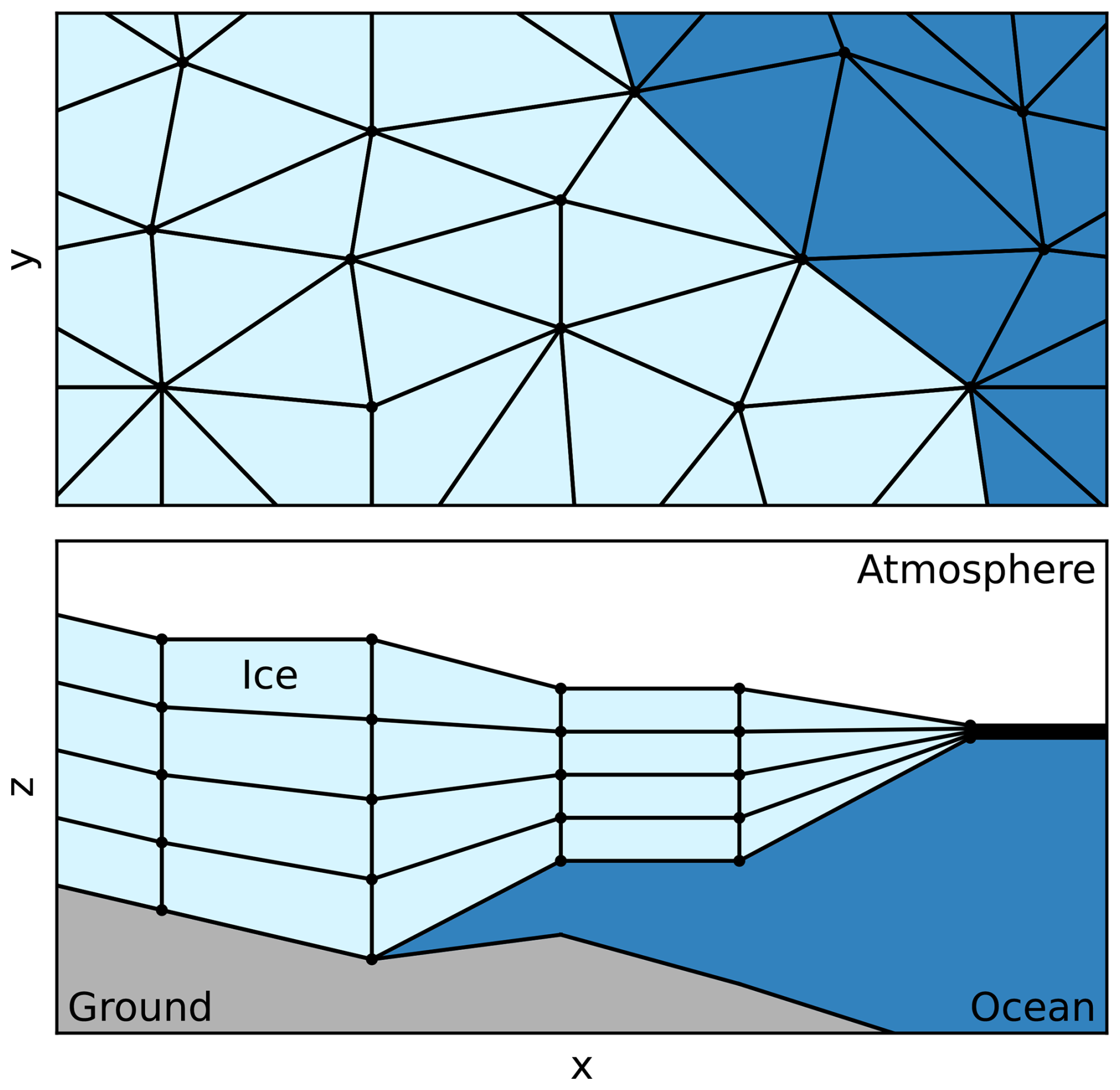
Figure 2 Schematic diagram of the ISSM mesh for 2D and 3D setups. The 2D mesh is an unstructured triangle grid covering the whole domain in the horizontal direction, even where there is no ice (top panel). Triangle elements are completely ice or completely ocean. The 3D mesh is generated by extruding the 2D mesh in multiple layers of triangle prism elements (bottom panel). The vertices in every layer have the same x and y coordinates. The z coordinate is set to match the ice's vertical extent and is updated when the ice thickness changes. In ice-free areas, the mesh collapses vertically to a minimum thickness.

For the SSA approximation, the 2D mesh is sufficient. For HO or FS, a three-dimensional mesh is required. The 3D mesh is generated by vertically extruding the 2D mesh in multiple layers. The vertices in the top layer are set at the surface of the ice. The vertices in the bottom layer are set at the base of the ice. The vertices in the layer in between are distributed between the top and bottom vertices, often with smaller spacing at the base. Therefore, the vertical (z) coordinate of the vertices changes in every time step as the thickness of the ice changes. The vertices are connected as truncated triangular prisms or tetrahedra.

ISSM uses the finite element method (FEM) to solve the partial differential equations (PDEs) for each core. The finite element type used can be configured for most cores individually. Linear P1 elements, where nodes are placed exclusively at the vertices, are the default for many cores, but higher-order elements are available.

All cores use the same mesh but generally do not have the same finite element types. The time stepping method and step size are also generally identical for every core with fixed or adaptive time steps, but a few cores, e.g., the hydrology core with the DoCo method (de Fleurian et al., 2016), subdivide the steps further. All cores use the same number of CPUs and the same domain decomposition for MPI parallelization. Fischler et al. (2022) showed that the cores that solve two-dimensional problems (e.g., mass transport, moving front) are significant bottlenecks for scaling as they compute fewer DOFs than the three-dimensional cores (e.g., thermal, stress balance).

2.2.3 Architecture

ISSM's architecture is well-suited for the development of a generic coupling adapter. Mesh and data access can be implemented based on abstract interfaces for different cores, mesh types, finite element types, etc. Variables are identified by runtime values (strings externally, mapped to enum values internally). With few exceptions, noted when describing the adapter in Sect. 2.3, the adapter does not need to include code to handle specific configurations.

2.3 The ISSM-preCICE adapter

The ISSM-preCICE adapter aims to be generic and extensible in order to support different use cases. This section explains how the features of ISSM and preCICE are handled in the implementation. The adapter is an executable that runs in place of the ISSM executable. The adapter configuration file is specified as a command-line parameter, and the command-line parameters of the ISSM executable are part of the adapter configuration file. The configuration of the adapter is done by a file in YAML format. The adapter configuration file is mostly responsible for mapping names specified in the preCICE configuration file to names expected by ISSM and defining the coupling interface. Listing 1 shows an example configuration file. The format conforms to the adapter configuration schema defined by the preECO project (https://precice.org/couple-your-code-adapter-software-engineering.html, last access: 22 May 2026). Details of the entries in the file are explained in the following sections. Each section highlights limitations and missing features.

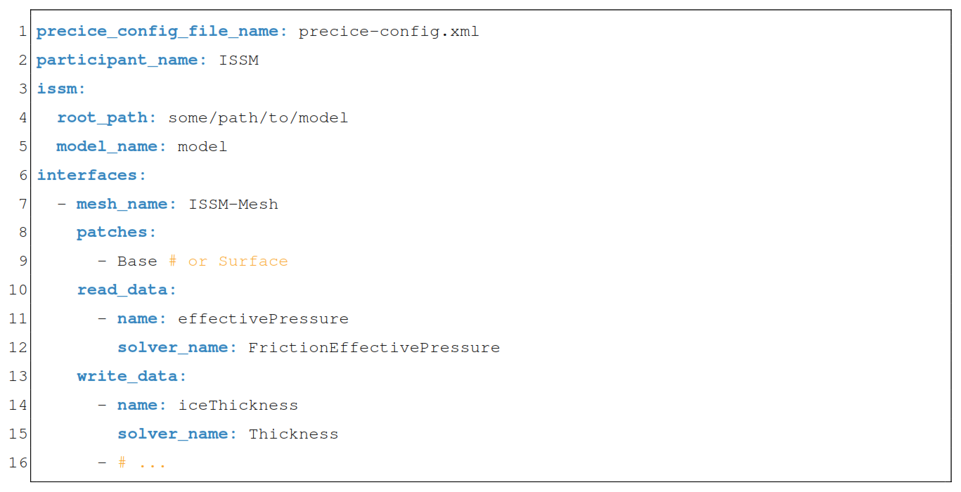
Listing 1 Example adapter configuration file in YAML format. The adapter requires information about the preCICE and ISSM configurations, the coupling mesh and the names of the variables being read or written. Variable names in the preCICE configuration file are mapped to variables known to ISSM.

2.3.1 Architecture of the adapter

Section 2.1.4 outlines the different ways to implement preCICE adapters. As shown in Fig. 3, the ISSM adapter is implemented as a coordinating wrapper application that calls ISSM (used as a library) as well as preCICE. This approach allows for independent development and a clean architectural separation between solver and adapter, allowing, e.g., easy support for multiple ISSM versions. However, this relies on a relatively stable API of ISSM and might pose maintenance challenges in the future. Additionally, due to the architectural choice of using ISSM as a library (instead of via its command-line interface), some functionalities internal to ISSM are not available. Note that so far, no changes to ISSM or its build process were necessary to support the features of the adapter.

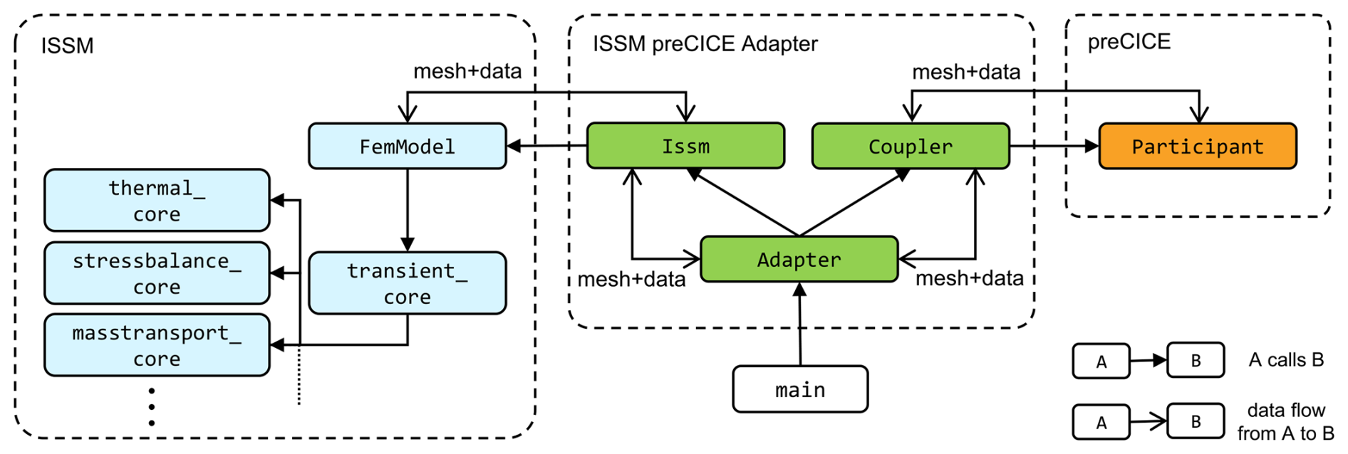
Figure 3 Structure of the ISSM-preCICE adapter. The adapter has its own time loop and calls the ISSM solver through the ISSM FemModel class. No interaction with the internals of ISSM (such as the constituent cores that make up the transient core) is necessary. The Adapter class is the entry point of the program; it coordinates the coupling and the exchange of coupled data (read and write) between ISSM and preCICE. Both ISSM and preCICE are wrapped in the adapter library to improve isolation and testability.

2.3.2 Coupling mesh

Since ISSM could potentially be coupled with many different codes, the coupling interface is configurable. The most important interfaces for coupling with the environment of the ice are the base and surface. So far, these are the only supported interfaces, see the list of limitations below for other interfaces that may be added later. In the configuration file, the user specifies which part of the mesh forms the coupling interface. The vertices of this part of the mesh are passed to preCICE. Mesh connectivity is added to support mapping schemes like linear cell interpolation (https://precice.org/configuration-mapping.html, last access: 22 May 2026) (Martin, 2022). The finite element representation of ISSM variables is evaluated at the mesh vertices before writing data to preCICE.

Some precision of high-order finite element types is lost when evaluating variables at the mesh vertices. Instead, the nodes of the finite elements could be used. For best results, this would require multiple coupling interfaces for different finite element types, and mesh connectivity would not be available. The adaptive mesh refinement feature of ISSM is not supported; the mesh must be static. Note that preCICE does provide facilities for mesh refinement (https://precice.org/couple-your-code-moving-or-changing-meshes.html, last access: 22 May 2026), but the adapter does not yet use them.

Specialized ESM couplers support masking of irrelevant areas, e.g., masking land for ocean models. As mentioned above, preCICE does not provide this feature. Additionally, preCICE does not handle non-matching domains very well. This is not a big issue for the use case discussed here, since ISSM and CUAS are interested in approximately the same domain, and both have internal mechanisms to exclude irrelevant areas and avoid wasteful computations. But it may be beneficial for, e.g., ice–ocean coupling to only couple over floating ice or coupling with a global atmosphere model.

3D (volume) coupling is a possible future extension. This would allow, e.g., to couple ISSM with itself to use different meshes for different cores to optimize precision or performance or to use an external thermal solver. However, as ice is transported by the solver, the z coordinate of the vertices changes in every time step. As the interface changes significantly over time, the coupling mesh could be reset to the new locations of the interface, just like for adaptive mesh refinement above. So far, we have not tested whether the computational overhead to update the coupling mesh and corresponding mapping matrices in preCICE is acceptable.

2.3.3 Variables

In ISSM, every state variable is identified by a unique name. These names do not follow any consistent convention, and the other coupling participant may use different names. So, it is necessary to map between names in the preCICE configuration file and ISSM names. The configuration file provides such name mappings for read and written variables.

If the ISSM setup uses a 3D mesh, the adapter can perform depth-averaging of a variable before writing it and extruding a variable (i.e., copying the variable values to the other layers of the mesh) after reading using the existing ISSM functionality.

ISSM accepts time series as input variables. For example, the user can set specific values for these variables at the beginning, middle, and end of the simulation. ISSM calls these “transient variables” and temporally interpolates between these values when necessary. However, ISSM does not allow overwriting the user-provided values of such transient variables. Therefore, the adapter requires coupled variables to be set up as non-transient, i.e., with one fixed value that is overwritten with the value read from preCICE during the simulation. This is a purely technical restriction and does not reduce modeling capabilities, since coupling also models input variables that change over time.

2.3.4 Data initialization

In ISSM, most variables are not zero as the simulation starts at some point in time in a defined state. For some variables, e.g., ice thickness, zero is not even valid at all. For non-zero initial values, preCICE requires data initialization (https://precice.org/couple-your-code-initializing-coupling-data.html, last access: 22 May 2026) by writing variables once at the beginning of the simulation. The ISSM adapter assumes that such initialization is necessary for every variable it writes.

For most variables, the adapter can simply write the initial value specified in the ISSM setup. However, users of stand-alone ISSM are not required to specify true initial values for variables that are computed by ISSM before they are used. For velocity, the initial value in the setup is merely used as an initial guess for the non-linear iteration of the stress balance core. Other variables, like rheology parameter B that is computed by the thermal core, do not need to be specified in the setup at all when the corresponding core is active.

For selected variables, the adapter can be configured to compute the true initial value. For example, to initialize velocity, the adapter would run the stress balance core once. But this is not possible for every variable, at least not in a generic way, so proper initial values must be provided by the user of the adapter even when it is not required by ISSM itself.

2.3.5 Boundary conditions

ISSM can set discrete Dirichlet boundary conditions (mainly called single point constraints in ISSM) for some cores, e.g., velocity (Vx, Vy, Vz) in the stress balance core. The adapter has limited support to set some of these constraints by coupling. In the ISSM code, the constraints are stored differently from normal variables, so generic support for all constraints that ISSM uses is currently not possible. The association between constraints and the core that they apply to has to be hard-coded for each one. For example, the adapter has no way to find out automatically that constraints on velocity are used by the stress balance core. Further complicating the implementation is that manual MPI communication is required in the adapter to synchronize constraints on ghost vertices. For variables, no such extra communication was necessary.

Constraints can currently only be coupled for P1 finite elements. Internally to ISSM, constraints are stored per finite element node, not per mesh vertex. But the coupling mesh is defined at the vertices instead of at the finite element nodes. Supporting constraints on other finite element types would require manual interpolation, whereas for normal variables, the interpolation from different finite element types is handled by ISSM automatically. Additionally, only velocity and pressure constraints of the stress balance core have been implemented so far.

2.3.6 Time stepping

ISSM performs multiple time steps per coupling window, depending on the step size set in the ISSM setup. During a coupling window, the adapter does not perform subcycling as it is defined by preCICE, i.e., it does not read or write intermediate values, only snapshots at the beginning or end. So, coupled variables are constant over one coupling window. The time interpolation features of preCICE mentioned in Sect. 2.1.3 are not currently used. This may be added in the future, but would probably require changes to the ISSM code. In the current version, the coupling window has to be set short enough to capture the dynamics of the system.

Implicit coupling is not supported. The adapter does not create the necessary checkpoints of ISSM, neither in memory nor on disk. Implicit coupling is required for numerical stability in some setups (see Sect. 2.1). Our experiments show no instability with explicit coupling. This is consistent with the internal explicit coupling of ISSM cores explained in Sect. 2.2.1. This is another possible future extension.

2.4 CUAS and the CUAS-preCICE adapter

CUAS-MPI (Fischler et al., 2023) is the MPI-parallel implementation of the Confined-Unconfined Aquifer System (CUAS) model for subglacial hydrology (Beyer et al., 2018). It employs an equivalent porous medium approach (e.g., Teutsch and Sauter, 1991), in which both distributed and channelized drainage are represented within a single porous layer. The model solves a vertically integrated groundwater equation (Fischler et al., 2023, Eq. 1) using effective quantities for storativity and transmissivity, which evolve based on parameterizations (Fischler et al., 2023, Eqs. 2–4). CUAS uses a finite difference spatial approximation on a regular rectangular grid and an implicit Euler time stepping scheme. CUAS solves for the hydraulic head that is proportional to the water pressure. The effective pressure, N (ice overburden pressure minus water pressure), is a diagnostic quantity that is computed at each time step and is used in ISSM for sliding.

We added an experimental preCICE adapter to CUAS. An adapter configuration file has not been specified yet, so the adapter is specific for coupling with ISSM. The adapter currently does not support implicit coupling schemes. It is implemented within the CUAS code base and is not a stand-alone application. This implementation approach is similar to, e.g., the CalculiX-preCICE adapter (Uekermann et al., 2017) and offers a high degree of flexibility. Additionally, the code base of CUAS is much smaller and more modern than that of ISSM, so maintenance is not significantly impacted by this choice.

Figure 4 shows an overview of the module structure and data flow. preCICE is integrated directly into the existing CUAS time step iteration, enabling subcycling and time interpolation. The CUAS-preCICE adapter consists of two parts. The Coupler class coordinates the main coupling operations of initialization, reading and writing data, and advancing the coupling window. It exchanges data with the CUAS model and solver through the SWAK4Coupling interface, which applies necessary transformations to the data based on the model physics. While some transformations are generic, e.g., deriving ice pressure used by CUAS from ice thickness provided by ISSM, others are very specific to the data that the ISSM-preCICE adapter can provide, hence the SWAK4ISSM specialization of the interface. Some of the tasks are as simple as converting rheology parameter B from ISSM to rateFactorIce (A) in CUAS using $A=B^{-\mathrm{3}}$ (assuming a Glen's flow law exponent of n=3). Others are more complex. For example, we use the ice thickness to compute the ice pressure. We further compute the pressure melting point using the ice pressure and the absolute temperature from ISSM to decide whether the ice is frozen at the bed or not, and adjust the mask (active versus inactive) in CUAS. Users can configure whether the mask is allowed to change based on the simulated temperature and the temperature threshold at which it becomes active. The transformations applied to the coupling data are implemented directly in the adapter, but the motivation is similar to preCICE Actions (https://precice.org/configuration-action.html, last access: 22 May 2026).

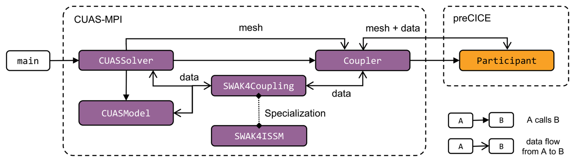
Figure 4 Structure of the CUAS-preCICE adapter. The coupling is integrated into and coordinated by the existing CUASSolver, but most of the coupling logic is isolated in added classes. The coupling data that is read and written flows through a utility class (specialized for coupling with ISSM) that handles transformations such as deriving ice pressure and transforming units.

Each time new data is available from preCICE (see Fig. 1), the CUAS-preCICE adapter needs to perform several tasks, which are briefly outlined below.

• iceThickness is translated into ice overburden pressure using ice density.

• groundedIceMeltingrate is rescaled from m s⁻¹ ice equivalent (IE) to m s⁻¹ water equivalent (WE) using ice and water density. This is then used as a time-independent (steady) forcing for CUAS during the duration of the current coupling time window.

• Use the iceThickness and the steady bed elevation field from CUAS to compute a new bndMask using the flotation condition. The bndMask contains the information where we have active hydrology (warm base, grounded ice) and where boundary conditions need to be applied (e.g. floating ice or open ocean). Here we also initialize grid points that turned from ocean into ice and thus active CUAS due to grounding line advance. Grounding line retreat is also handled.

• We use iceLevelset to disable grounded ice areas in the CUAS domain that are not part of the ISSM domain. We do not use oceanLevelset in the prototype implementation of the adapter.

• basalTemperatureIce together with iceThickness is used to decide if the base is at the pressure melting point to further constrain the bndMask in CUAS, if needed.

• The basalVelocityIce is copied over without modifications.

• Finally, rateFactorIce (A) in CUAS is computed based on basalRheologyB.

Because the effective pressure is computed directly in CUAS, the adapter can provide this field for coupling without further modifications. We use iceThickness instead of iceLevelset and oceanLevelset provided by ISSM to define the bndMask in CUAS. This ensures that the grounding line (GL) in CUAS is consistent with the local bed topography. The ISSM mesh resolution at a given location may be substantially coarser than the CUAS grid resolution. Through the preCICE coupler, we only receive interpolated level-set fields representing the GL position on the coarser ISSM mesh. Consequently, the transferred GL location may not align with the grounding line implied by the higher-resolution bed topography used in CUAS.

To enable coupled simulations, the model capabilities of CUAS, beyond the adapter, have been further enhanced. Simulations of the Greenland Ice Sheet require water not only from the basal melt computed by ISSM, but also from surface runoff. Until now, there has been only one input field and a corresponding internal storage field for the combined water from all sources, used as model forcing. We added the ability to store multiple water sources that can be changed independently (by a time series from input files or by coupling) and added up when required. Various parameters, such as water and ice density, that were compile-time constants are now configurable at runtime to match the parameters set in ISSM.

3 Experiments

This section presents experimental verification of the ISSM-preCICE adapter for coupling ISSM to CUAS. First, we demonstrate functionality using a synthetic setup, then we analyze the performance using preexisting large-scale setups of the Greenland Ice Sheet.

3.1 Functionality

We ran simulations with a synthetic setup. The simpler geometry compared to a real-life setup allows us to verify the correctness of the implementation and study the complex behavior of the coupled system in a more controlled setting.

3.1.1 Experimental setup

We use the synthetic Thule geometry developed for the CalvingMIP project (Jordan, 2024). This setup is based on analytical functions for the bed elevation and yields an ice-sheet geometry that encompasses all major components of an ice-sheet model domain (grounded ice, floating ice, and open ocean). In CalvingMIP it is used to study how different ice sheet models handle calving in a very controlled setup. Instead of fixed thermal and friction conditions as in the original definition, we enable the thermal core of ISSM with surface temperature 250 K and geothermal flux 0.05 W m⁻² to compute basal melt rates to be used by CUAS and we use the default Budd friction law $\left({\mathit{\sigma }}_{\mathrm{b}}=-C^{\mathrm{2}}{N}^{\frac{q}{p}}|{\mathit{v}}_{\mathrm{b}}{|}^{\frac{\mathrm{1}}{p}-\mathrm{1}}{\mathit{v}}_{\mathrm{b}}\right)$ with coefficient C=100, exponents p=3 and q=2, and effective pressure N supplied by CUAS. Surface mass balance was increased to 8 m yr⁻¹ IE. The goal is to have a balanced geometry with grounded and floating, fast- and slow-flowing regions to assess the effects of coupling.

The combined model (ISSM + CUAS) spin-up consists of two phases. First, we run the ISSM model for 12 000 years with a time step of 0.1 year to reach a steady state, using an effective pressure equal to the ice overburden pressure. In the second phase, CUAS and ISSM run coupled without melt runoff forcing, exchanging data every 0.1 year (equal to the ISSM time step) for 200 year. This allows CUAS to find its own steady state while keeping ISSM state consistent with the effective pressure computed by CUAS.

For the actual experiment, we add forcing in the form of seasonal and spatially varying meltwater runoff (in addition to the basal meltwater received from ISSM) to CUAS to induce a dynamic system. We ran simulations with low and high runoff. The peak forcing in summer (day 210 of the year) in areas with ice surface below 500 m is 0.2 m yr⁻¹ WE for low runoff and 2.0 m yr⁻¹ WE for high runoff. Over the year, the forcing follows the shape of a Gaussian distribution with parameters μ=210 d and σ=20 d. Spatially, forcing is maximal in areas of low ice surface elevation (h_s<500 m) and zero in areas of high ice surface elevation (h_s>1500 m). For medium ice surface elevation, forcing follows a monotone cosine curve, i.e., it increases continuously as the surface elevation decreases. The surface elevation h_s is taken at the end of the spin-up, the forcing is not dynamically updated.

The basic coupling configuration, both for spin-up and the following experiment, is shown in Fig. 1. As described above, CUAS writes the effective pressure that is used by ISSM to determine basal friction. The basal melting rate from ISSM provides a water source for CUAS. Basal temperature, ice thickness, and ice and ocean masks are used to update the active CUAS mask. The temperature threshold for activating the mask is set to 269.15 K. Ice velocity and rheology govern channel opening and closure, represented in CUAS by increasing and decreasing transmissivity, respectively. We use linear cell interpolation to map data between the two meshes. Details on how the coupled variables are used in CUAS are described in Sect. 2.4. Simulations are run over two years to assess changes from one year to the next. Data is exchanged daily to accurately capture rapid changes during summer. ISSM uses time steps of 1 d same as the coupling window, CUAS 4 h.

We compare a fully coupled (2-way) run with one in which coupling is performed only in one direction (1-way). In 2-way, ISSM and CUAS exchange all variables as per the coupling configuration described above. In 1-way, ISSM receives the updated effective pressure from CUAS, but CUAS does not receive updated ice geometry from ISSM. This is equivalent to offline coupling: first run CUAS stand-alone, then use the resulting time series as input for a stand-alone ISSM simulation. To ensure comparable aggregate forcing, CUAS receives the steady basal melt field from the end of the spin-up from an input file.

3.1.2 Results

The state at the end of the combined model initialization (spin-up) is presented in Fig. 5. The ice thickness and basal velocity are selected as the key quantities describing the ice sheet state, while effective pressure and subglacial discharge are selected to describe the state of the subglacial hydrology. The dark gray areas in Fig. 5a–d (and subsequent maps) indicate the grounded parts of the domain where basal temperatures from ISSM are below the pressure melting point, and ice sheet basal melt is zero (cold base) and hence no active hydrology exists. The ice thickness (Fig. 5a) in the warm-based area varies over several thousand meters, with low thickness in region A and along the northern and southern grounding lines, as well as the upstream end in region B. The effective pressure (Fig. 5b) is lowest at the grounding line and reaches magnitudes above 6 MPa. Basal velocities (Fig. 5c) range from 10 to about 400 m yr⁻¹ with the largest values along the long grounding lines in the north and south. Along those grounding lines, the subglacial discharge (Fig. 5d) is highest, with a similar pattern of N, v_b and D.

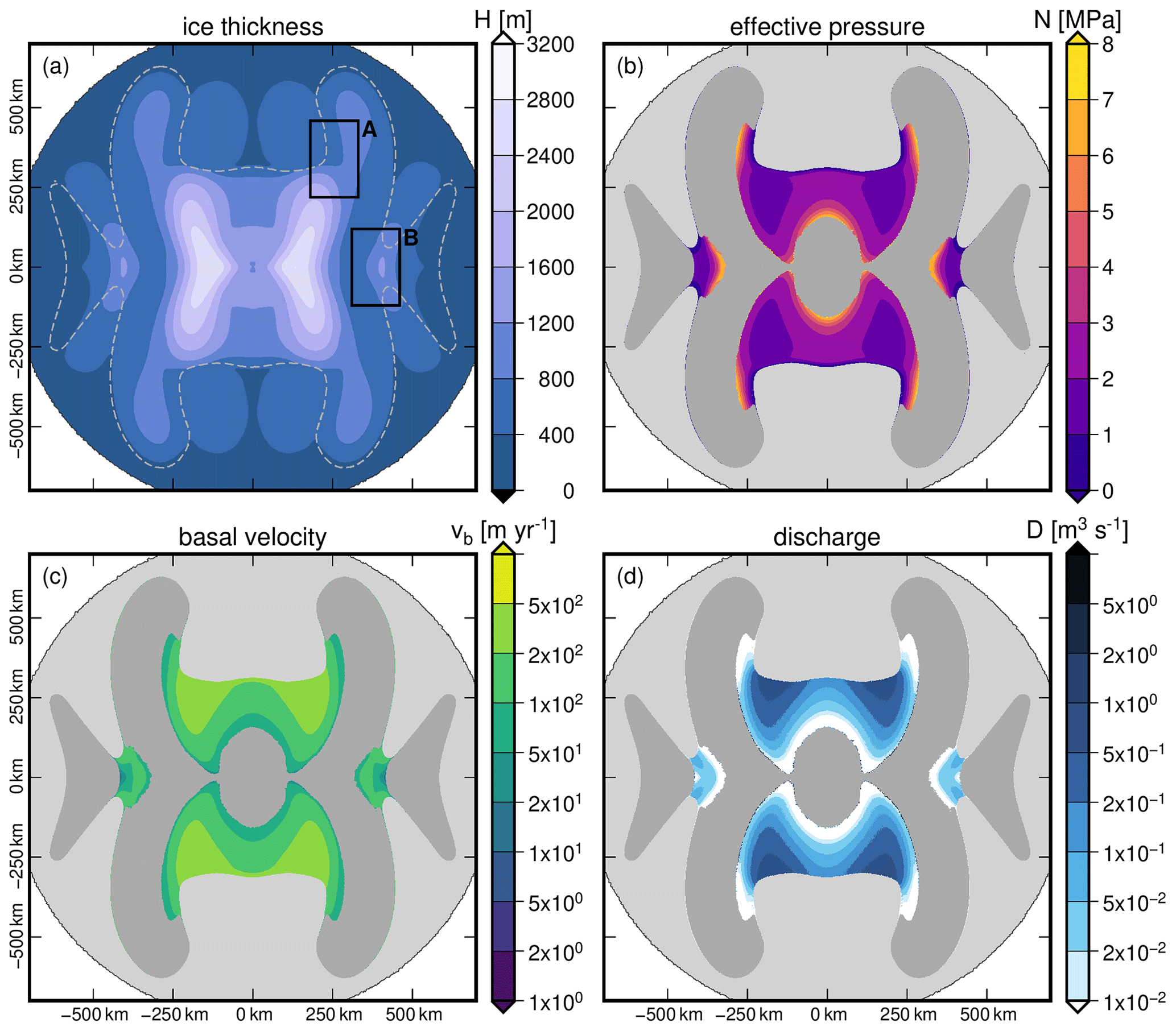
Figure 5 Model state at the end of the spin-up for the Thule domain setup. Ice-dynamical fields are shown in the left column: (a) ice thickness and (c) basal velocity. Subglacial hydrological fields are shown in the right column: (b) effective pressure and (d) subglacial discharge. Ice thickness in (a) is shown over the full plotted extent, while all other fields are shown only for the grounded ice area. The grounding line is indicated in (a) by a dashed line. In panels (b)–(d), floating ice shelves are shown in light gray, and dark gray areas indicate grounded regions that are inactive in CUAS. The maps are cropped relative to the full computational domain to focus on the grounded ice region. Rectangles (A, B) indicate regions of high activity referenced in the text.

For a further investigation of the differences in 1- and 2-way coupling, we present simulations with different magnitude in seasonal forcing. Figure 6 displays the time series of total water source, Q_tot, mean effective pressure, $\overline{N}$, mean effective transmissivity magnitude, $\stackrel{\mathrm{‾}}{\log \left(T_{\mathrm{e}}\right)}$, and basal velocity magnitude, $\stackrel{\mathrm{‾}}{\log \left(v_{\mathrm{b}}\right)}$ showing 1-way and 2-way coupling and for each full forcing (high) and only 10 % amplitude forcing (low). The imposed runoff forcing is periodic with a one-year period and attains its maximum at day 210, end of July. As model output is written every 10 d, this maximum is not sampled exactly in the second simulation year. The nearest stored time step (day 215), therefore, exhibits a slightly reduced signal amplitude. The effective pressure (Fig. 6b) has a lower difference between 1- and 2-way coupling for low runoff forcing. In both runoff cases, the 2-way coupling has higher $\stackrel{\mathrm{‾}}{N}$. The timing in $\stackrel{\mathrm{‾}}{N}$ is slightly delayed to Q_tot due to the low runoff forcing. The timing of $\stackrel{\mathrm{‾}}{\log \left(T_{\mathrm{e}}\right)}$ (Fig. 6c) in the low runoff forcing is similar to $\stackrel{\mathrm{‾}}{N}$ and $\stackrel{\mathrm{‾}}{\log \left(v_{\mathrm{b}}\right)}$ (Fig. 6d). The effect of the coupling is small for low runoff forcing in $\stackrel{\mathrm{‾}}{\log \left(T_{\mathrm{e}}\right)}$, with larger differences outside the peak runoff and higher $\stackrel{\mathrm{‾}}{\log \left(T_{\mathrm{e}}\right)}$ in 1-way. The basal velocity resembles the inverse shape of $\stackrel{\mathrm{‾}}{N}$.

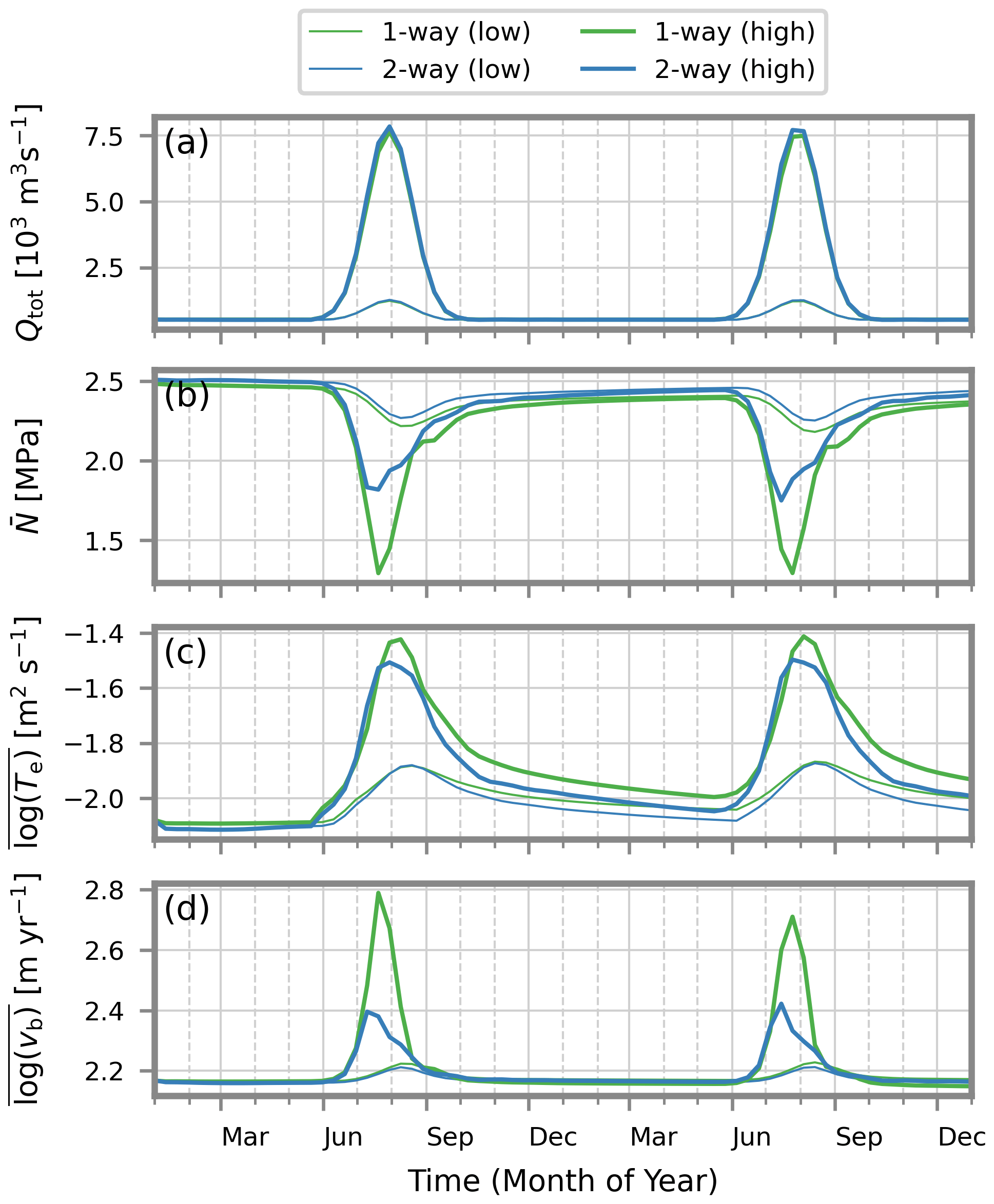
Figure 6 Time series of total water source Q_tot, mean effective pressure $\stackrel{\mathrm{‾}}{N}$, mean effective transmissivity magnitude $\stackrel{\mathrm{‾}}{\log \left(T_{\mathrm{e}}\right)}$, and mean basal velocity magnitude $\stackrel{\mathrm{‾}}{\log \left(v_{\mathrm{b}}\right)}$ for the four simulations: one-way coupling in green, two-way coupling in blue; high-amplitude forcing shown with thick lines, low-amplitude forcing with thin lines. The means are evaluated as spatial means on the time-dependent active CUAS mask.

Comparing the results for 1-way and 2-way coupling in ice thickness difference (Figs. 7a and 8a), we find distinct differences in the regions A and B: in A the 1-way case exceeds ±50 m, while the 2-way case has small differences. The pattern of ice thickness difference is similar for the 1-way and 2-way coupling, but the magnitude is significantly larger in the 1-way case. For both 1-way coupling and 2-way coupling, we find a reduction in effective pressure compared to the spin-up that does not contain seasonal runoff (Figs. 7b and 8b). In both 1-way and 2-way coupling, we have an increase in basal velocity compared to the spin-up (Figs. 7c and 8c), with an extreme increase in region A for the 1-way coupling. The discharge (Figs. 7d and 8d) is in both cases larger than in the spin-up, but the difference to the spin-up is only moderate in magnitude, except for region B in the 1-way case.

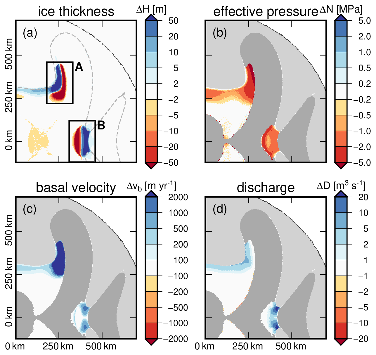
Figure 7 Results of the one-way coupled simulations using the Thule setup. Panels (a)–(d) show differences in the summer state (day 215 of year two) relative to the end of the spin-up. The panel layout is identical to Fig. 5, with ice-dynamical fields in the left column (a, c) and subglacial hydrological fields in the right column (b, d). Differences are evaluated on the common grounded domain, except for panel (a), where ice thickness differences are shown wherever ice thickness is defined. The maps show approximately one quarter of the model domain, exploiting symmetry along both horizontal axes. Rectangles (A, B) indicate regions of high activity referenced in the text.

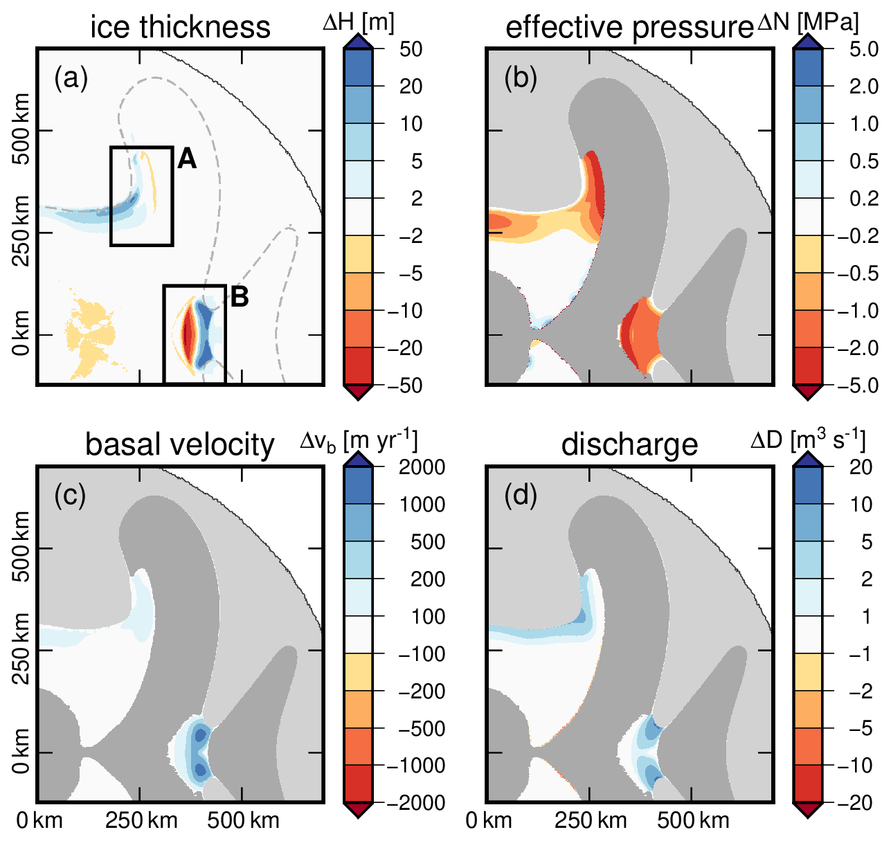
Figure 8 Result of the fully coupled (two-way) simulations using the Thule setup. Panels (a)–(d) show differences in the summer state (day 215 of year two) relative to the end of the spin-up. The panel layout is identical to Fig. 5, with ice-dynamical fields in the left column (a, c) and subglacial hydrological fields in the right column (b, d). Differences are evaluated on the common grounded domain, except for panel (a), where ice thickness differences are shown wherever ice thickness is defined. The maps show approximately one quarter of the model domain, exploiting symmetry along both horizontal axes. Rectangles (A, B) indicate regions of high activity referenced in the text.

3.2 Performance

The coupled simulation should run with minimal computational overhead and use computing resources efficiently. To demonstrate this, we use a large-scale setup of the Greenland Ice Sheet as the simple setup used in Sect. 3.1 is not complex enough to have performance characteristics that are representative of real uses cases, which usually have much more complexity. We have analyzed the performance of initialization and data mapping, as well as scaling with the number of processes.

3.2.1 Experimental setup

The setup for ISSM is mostly the same as G1000 in Fischler et al. (2022). The only modification we made for this paper is to use the default ISSM Budd friction law ${\mathit{\sigma }}_{\mathrm{b}}=-C^{\mathrm{2}}{N}^{\frac{q}{p}}|{\mathit{v}}_{\mathrm{b}}{|}^{\frac{\mathrm{1}}{p}-\mathrm{1}}{\mathit{v}}_{\text{b}}$ with coefficient C=12.94, exponents p=3 and q=2, and effective pressure N provided by CUAS. The spin-up process is the same as in Fischler et al. (2022). During the spin-up, the effective pressure is $N=N_{\mathrm{opc}}={\mathit{\rho }}_{\mathrm{ice}}gH-\max (\mathrm{0},{\mathit{\rho }}_{\mathrm{water}}g(-z_{\mathrm{b}}\left)\right)$ with z_b the height of the base above sea level as in Wolovick et al. (2023). The setup set the lower bound for effective pressure 35 % of ice overburden pressure. This parameter is likely to affect the stability of the coupled system, but investigating its effect in detail is beyond the scope of this work. The resolution of the mesh is around 0.7 km at the shear margins, 10 km at slow-moving ice in the interior, and up to 100 km at open ocean.

The CUAS setup is taken from Fischler et al. (2023). We use G600, which has a uniform grid with 600 m resolution, similar to the minimum element size of the ISSM mesh. We use daily surface runoff data (R) from the regional climate model RACMO (Noël et al., 2019) for the year 2019 in addition to the ice sheet basal melt (M) from ISSM to impose seasonality to the CUAS water source as:

$$\begin{array}{}\text{(1)}& Q(x,y,t)=M(x,y,t)+\mathrm{0.9}R(x,y,t),\end{array}$$

where we only consider 90 % of the surface runoff to enter the subglacial system. The percentage is arbitrary, but ensures strong seasonality for the coupled simulations. In the year 2019, particularly high melt was measured for the Greenland Ice Sheet (Tedesco and Fettweis, 2020; Sasgen et al., 2020). The aquifer layer thickness in CUAS was chosen equal to 1 m, with yield storativity $S_y={\mathrm{10}}^{-\mathrm{2}}$ and minimal transmissivity $T_{\min }={\mathrm{10}}^{-\mathrm{14}}$ m² s⁻¹. Subglacial channel creep opening/closure is parameterized using an ice flow rate factor of $A=\mathrm{6.8}\times {\mathrm{10}}^{-\mathrm{24}}$ Pa⁻³ s⁻¹ (Werder et al., 2013). All remaining parameters are unchanged from those reported in Fischler et al. (2023). For defining the initial active mask in CUAS, a threshold of minimum 10 m of ice thickness was chosen. The temperature threshold for activating the mask during simulation is set to 269.15 K. Similar to ISSM, the initial hydraulic head of CUAS is derived from N_opc.

The preCICE coupling configuration is the same as in Sect. 3.1 with the exception of using different mapping methods for Sect. 3.2.4 and different coupling schemes for Sect. 3.2.3. Simulations run for 730 d.

For the measurements, we are using the profiling utility integrated into preCICE (https://precice.org/tooling-performance-analysis.html, last access: 22 May 2026). The runtime of initialization is measured at the beginning. Where we report aggregate runtime of solvers or data mapping in the following sections, only the final 365 days are included. This ensures that the analysis includes a full year of seasonal changes but excludes the noisy early-coupling windows in which the states of ISSM and CUAS are not yet aligned. In real use, depending on which parameters are changed between runs, this relaxation phase could be skipped entirely by using restart files. Runtime measurements do not include writing output, as I/O execution times can swing wildly and unpredictably. Adding moderate amounts of data output to both participants should not, on average, significantly impact the analysis. Every experiment is repeated three times, and the results are averaged to reduce variance.

In parallel coupling schemes, every participant has its own exclusive resources. CPUs are assigned according to a ratio $\mathit{\alpha }=n_{\mathrm{ISSM}}/n_{\mathrm{CUAS}}$ where n_S is the number of CPUs assigned to solver S. Care is taken to assign packed CPU blocks to participants, i.e., processes used by one participant are as local to the nodes as possible, since each participant communicates more internally than with other participants.

In serial coupling schemes, we conducted experiments with both shared and exclusive resources. Shared resources are used by both solvers in turn. Exclusive resources are used by only one solver and are idle while the other solver computes. That means, except during initialization, half of the CPUs will be almost completely idle. Little energy is wasted, but the cluster resources are nonetheless reserved for the entire run. With shared resources, both solvers always use all allocated CPUs, as it is generally recommended to use all allocated cluster resources unless the region of flat or negative scaling is reached. For better comparisons, we also allocate the same number of CPUs to both solvers when using exclusive resources.

Where we give CPU or process counts below, they have the following meanings for the coupling and resource allocation schemes:

• Parallel: total number of processes allocated to both solvers, each solver using a fixed subset.

• Serial (shared): total number of processes allocated, used by both solvers in turn.

• Serial (exclusive): maximum number of processes allocated to either solver. Since the processes of the other participant are mostly idle, this results in the most relevant comparison regarding the required resources and it allows us to measure the effect of resource contention. As both solvers use the same number of processes, the number of processes given in plots is half the number of processes allocated.

All experiments are performed on the Albedo cluster of the Alfred Wegener Institute. The compute nodes of the cluster are equipped with 256 GB of RAM and two AMD Rome Epyc 7702 CPUs for a total of 128 CPU cores per node and are connected by 100 GB InfiniBand network. The solvers and dependencies are built with GCC version 12.1.0 and OpenMPI version 4.1.3.

3.2.2 Initialization

In Earth System Models, initialization time of the solvers and the coupling library is of significant concern. For this scaling analysis, we use nearest neighbor mapping exclusively. Comparison of mapping methods follows in Sect. 3.2.4.

Figure 9 shows the time required to initialize preCICE. This includes establishing connections between participants and processes, partitioning of the domain, and computation of mapping weights. We do not analyze these parts separately, as it would require too much explanation of preCICE internals, and we are primarily working from the point of view of a preCICE user. For comparison, Figs. 10 and 11 show the time required to initialize the solvers. Note that ISSM and CUAS initialize at the same time, so the actual time required is the maximum of both. While the data is quite noisy due to a low number of repetitions and high variance of I/O, general trends can be identified.

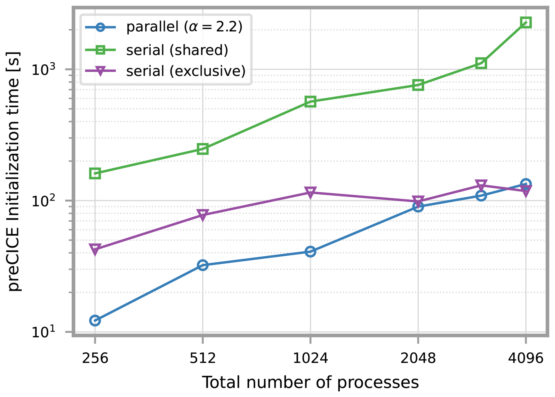
Figure 9 Time to initialize preCICE in the Greenland setup for different coupling and/or resource allocation schemes and increasing numbers of processes. For the parallel coupling scheme, CPUs are allocated to ISSM and CUAS at a ratio of $\mathit{\alpha }=n_{\mathrm{ISSM}}/n_{\mathrm{CUAS}}=\mathrm{2.2}$. The serial coupling scheme can be run with exclusive CPUs for each participant or with shared resources that are used in turn. Initialization includes partitioning of the coupling mesh and computation of nearest neighbor mapping weights for both solvers.

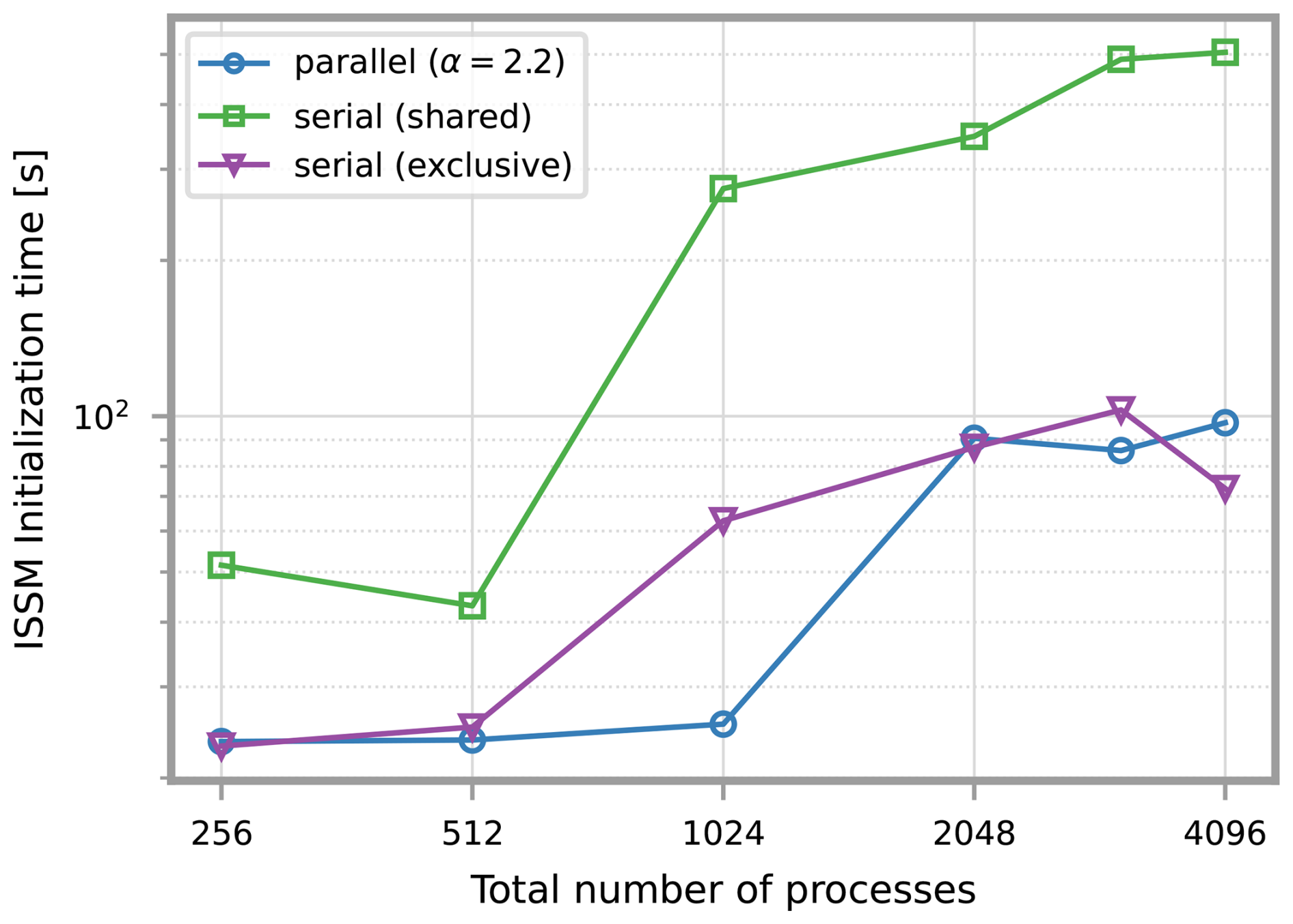
Figure 10 Time to initialize the ISSM Greenland setup for different coupling and/or resource allocation schemes and increasing numbers of processes. Initialization consists mostly of loading of input data from files.

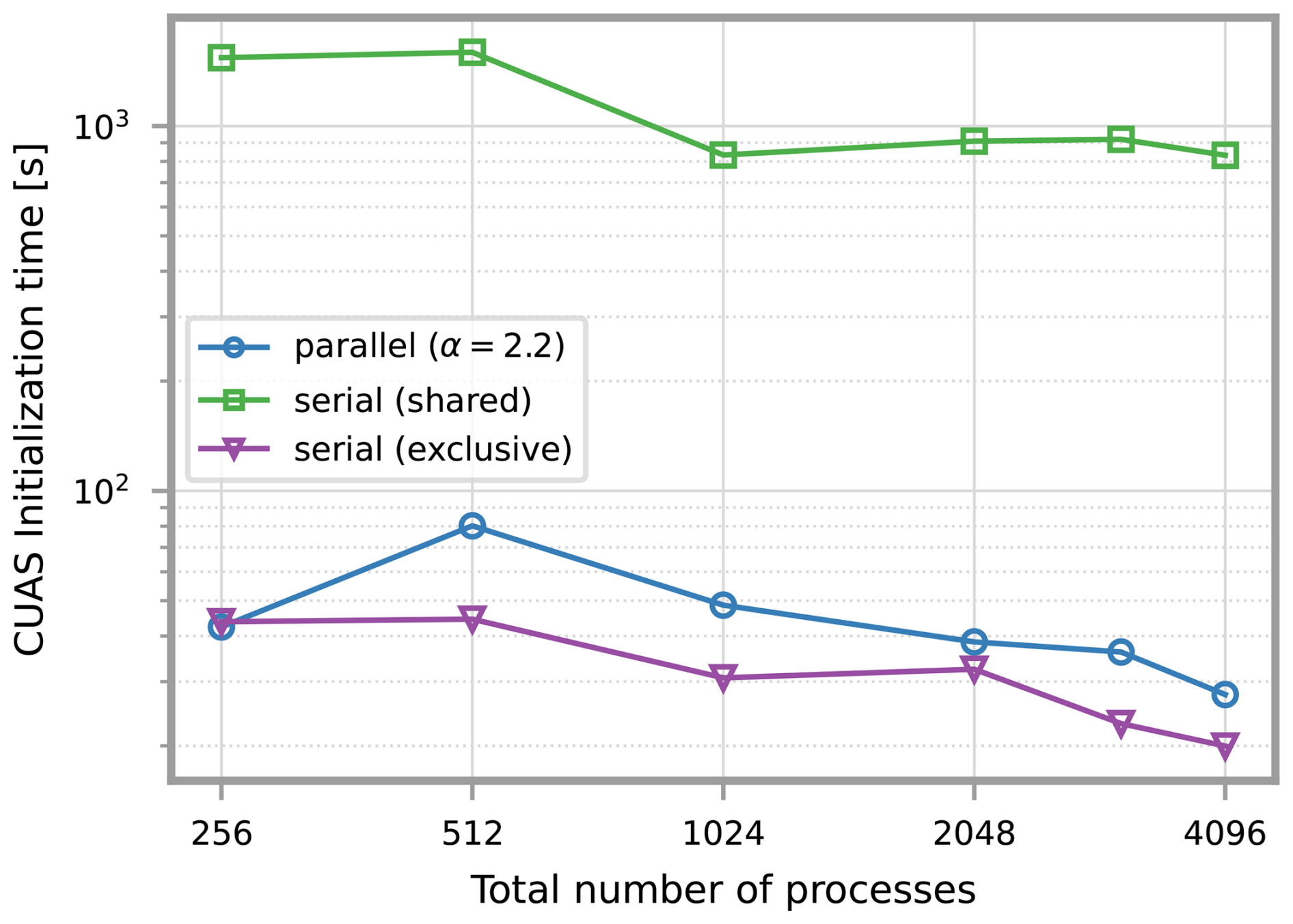
Figure 11 Time to initialize the CUAS Greenland setup for different coupling and/or resource allocation schemes and increasing numbers of processes. Initialization consists mostly of loading of input data from files.

ISSM initialization time grows linearly with the number of processes. CUAS is basically constant, trending slightly downward. Solver initialization is dominated by CUAS at low CPU counts. The larger mesh means higher data input requirements. ISSM catches up between 1024 and 2048 processes due to less optimal parallel I/O accesses.

In the range of CPU counts tested, preCICE initialization times also grow linearly with the number of processes, as more communication is necessary to partition the meshes and compute weights. Initializing the coupler and initializing the solvers requires similar time, except in the case of serial coupling with shared resources.

Sharing resources during initialization in serial coupling has a strong negative effect. Naive estimation would suggest the required time doubles for shared resources, since the same amount of work is being done by half the CPUs. However, scheduling conflicts can increase times by an order of magnitude or more. CUAS is especially badly affected, probably due to contention of I/O resources. Parallel and serial exclusive require approximately the same amount of time. The increased effort required to compute and communicate the weights of a more partitioned mesh is counterbalanced by the increased resources.

3.2.3 Simulation

For parallel coupling, we first needed to determine the optimal distribution of available CPUs among the solvers. This is the ratio of CPUs used by ISSM and CUAS where both solvers take approximately the same time for one coupling window. Figure 12 a shows the times required to compute a single coupling window with different distributions of 256 total CPUs. The best result is at α=2.2. If both participants scale equally, this would be the ideal distribution for larger numbers of CPUs as well.

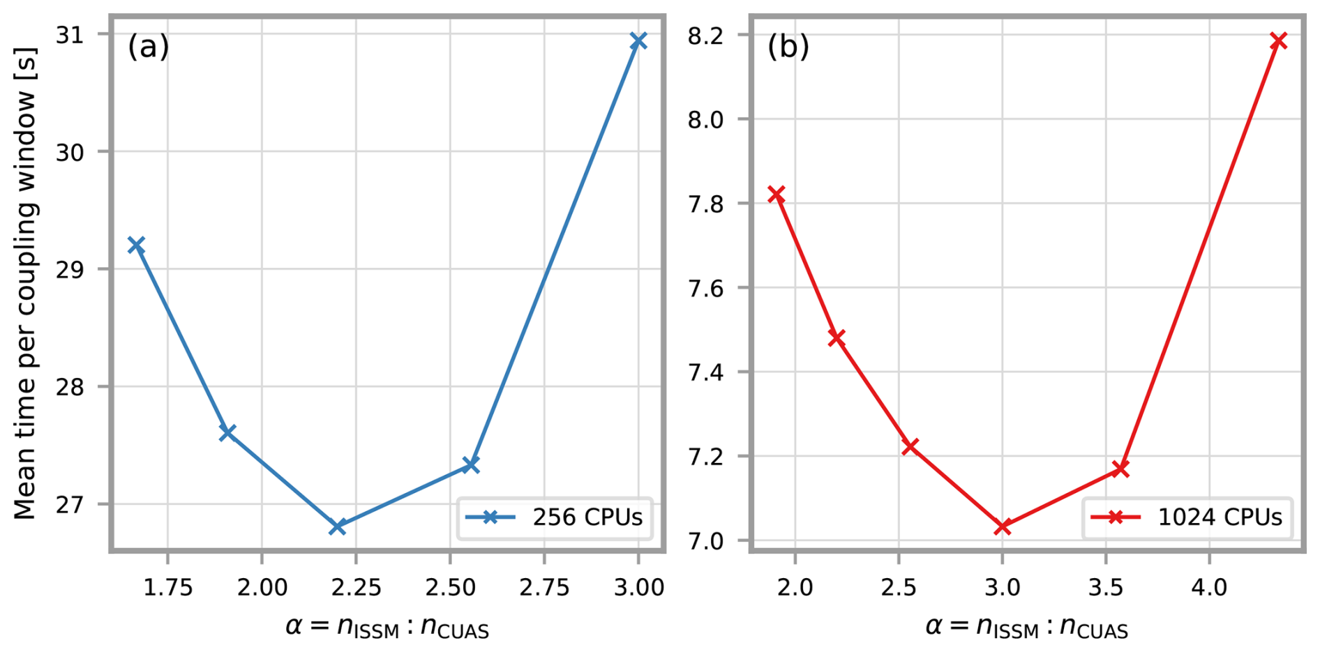
Figure 12 Average time to compute one coupling window with parallel coupling scheme in the Greenland setup for different distributions of 256 (a) and 1024 (b) total CPUs.

However, as Fig. 13 displays, ISSM does not scale as well as CUAS. This is consistent with the scaling analyses of stand-alone ISSM (Fischler et al., 2022) and CUAS (Fischler et al., 2023) as well, even though the uncoupled and coupled solvers are not directly comparable. Accordingly, with increasing numbers of processes, the duration that CUAS waits for ISSM increases as shown in Fig. 14. At 256 processes, where the distribution of α=2.2 had the best result, the wait times are close. Note that even here, the wait time is not zero, as the computational effort of each solver varies with the seasons, and both solvers wait in some coupling windows.

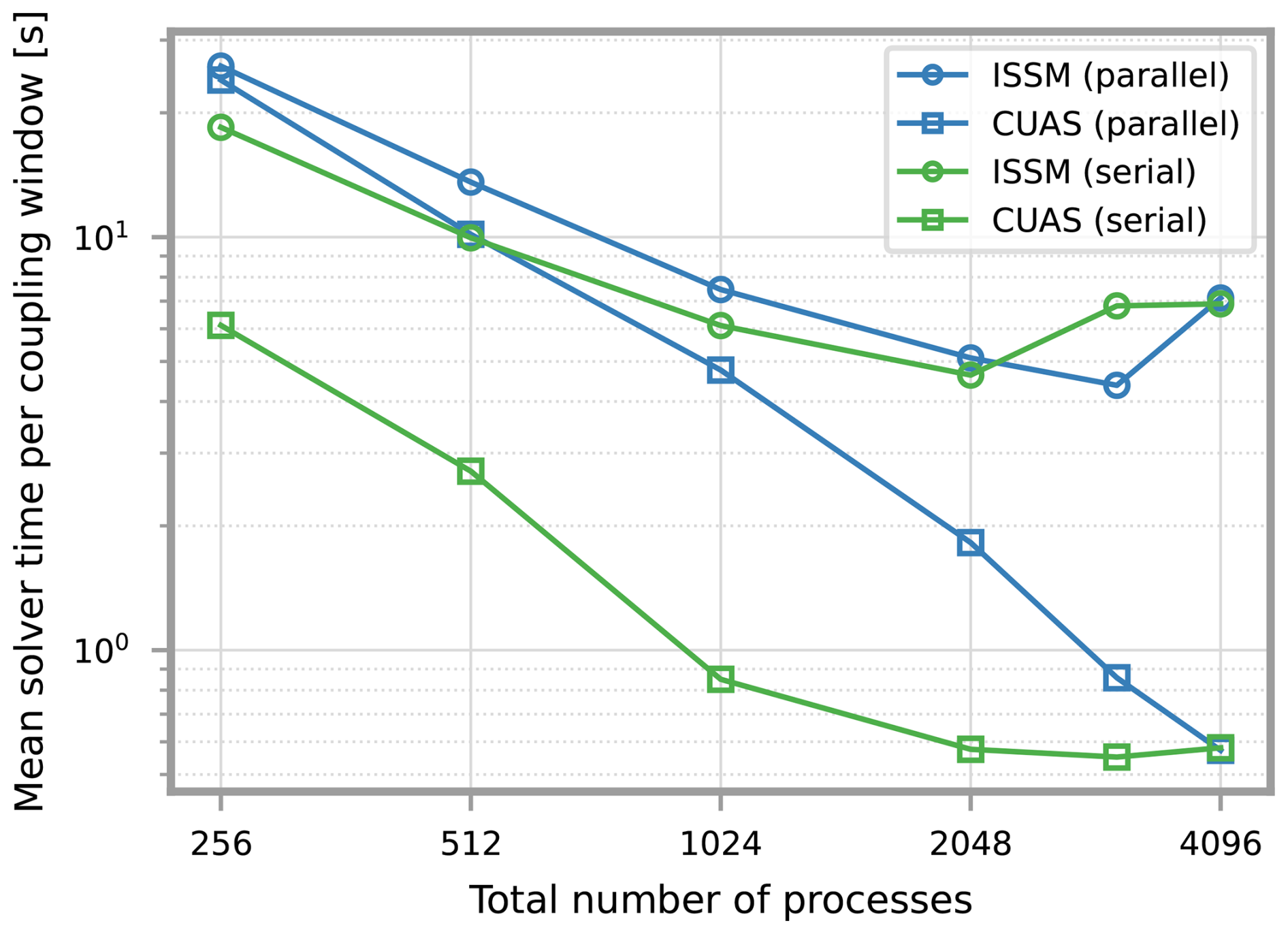
Figure 13 Average execution time required by the CUAS and ISSM solver during one coupling window for CUAS and ISSM in the Greenland setup for increasing numbers of MPI processes.

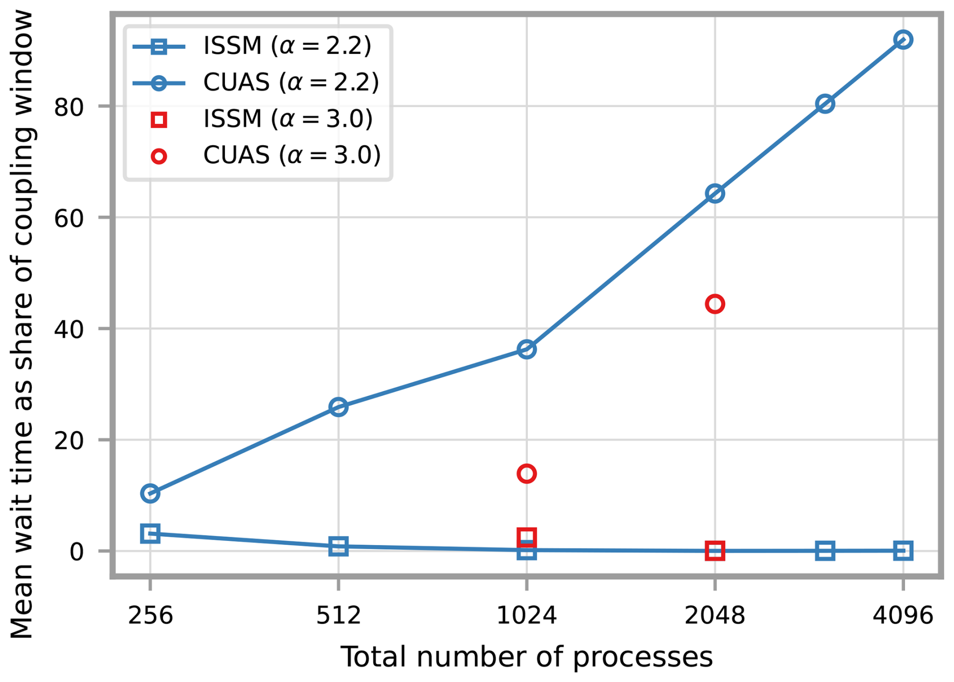
Figure 14 Average wait time relative to execution time of one coupling window for CUAS and ISSM in the Greenland setup in a parallel coupling scheme for increasing numbers of MPI processes and two different distributions of processes to participants.

These results suggest that more than 256 CPUs should be distributed differently. Figure 12b shows that for 1024 processes, the ideal distribution would be α=3.0. Figure 14 shows reduced wait times for this distribution over α=2.2. Note that when running the simulation once at any moderate distribution α and measuring the average solver runtime t_X, the equation ${\mathit{\alpha }}_{\mathrm{opt}}=t_{\mathrm{ISSM}}/t_{\mathrm{CUAS}}\cdot \mathit{\alpha }$ gives a decent approximation of the optimal distribution. For example, with α=2.2 and the measured solver times t_ISSM=7.5 s and t_CUAS=4.8 s, the estimated optimal distribution is α_opt=3.4, which is close to the minimum in Fig. 12b.

With these preparations, we ran scaling experiments of the coupled system. Figure 15 shows a comparison of average run times for a coupling window for parallel and serial coupling schemes with different resource allocations.

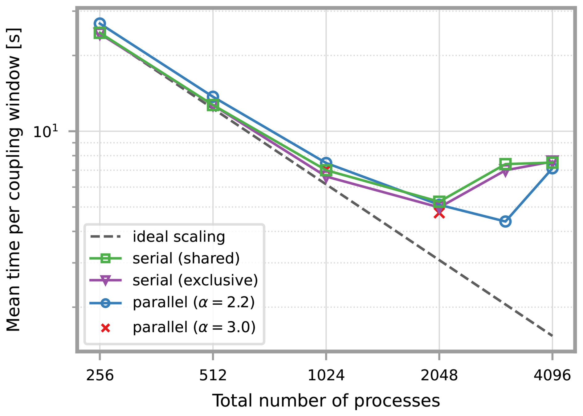
Figure 15 Average execution time for one coupling window (includes solver, communication, and data mapping) using a parallel or serial coupling scheme in the Greenland setup for increasing numbers of MPI processes. Parallel coupling is tested with different distributions of processes to participants, serial coupling with exclusive or shared resources.

In the lower range of processes, where both serial and parallel show almost ideal scaling, serial coupling is slightly faster. There is an unexpected bend in the measured times for serial coupling. The same bend is observed in the ISSM solver execution times, but not in CUAS. We were unable to identify the root cause or any difference in the simulation that could explain it, the number of solver iterations is similar between all experiments. A deeper analysis of the ISSM solver is beyond the scope of this work.

Exclusive resources for serial coupling give a small advantage over shared resources, but probably insignificant compared to the difference in initialization times discussed in Sect. 3.2.2. Scaling is basically identical. The changed distribution of CPUs in parallel coupling also gives a small advantage over the original distribution.

3.2.4 Mapping

preCICE offers a choice of different methods for mapping data between meshes. The methods differ in the order of approximation and computational cost. We ran experiments with a selection of three methods of different order:

• nearest neighbor (NN), a first order projection method

• linear cell interpolation (LCI), a second order projection method using barycentric coordinates

• partition-of-unity radial basis functions (PoU), a kernel based method designed for large scale mappings

We tested all mapping methods with a parallel coupling scheme on 1024 total CPUs, distributed 2.2:1 to ISSM and CUAS and measured the initialization time and mapping time per coupling window.

The PoU method and basis functions must be parameterized (https://precice.org/configuration-mapping.html, last access: 22 May 2026). Our setup is particularly challenging for the current, relatively recent implementation of PoU in preCICE. As described in Sect. 3.2.1, the ISSM mesh has a wide range of element sizes. However, preCICE currently permits only a single global parameter each for the basis function radius and PoU cluster size. In addition, the fields of an ice sheet model include discontinuities at the calving front and grounding line. Even with the best parameterization we found (C0 compact polynomial basis functions, radius 200 km for mapping from ISSM to CUAS, 10 km from CUAS to ISSM, default values for the other parameters), there is overshooting, e.g., negative ice thickness values all around the ice boundary as in Fig. 16. Performance measurements are included here with the hope that improvements in preCICE and/or the setup will be implemented. The other methods did not show such problems, detailed analysis of numerical errors is beyond the scope of this work but is covered in Chourdakis et al. (2022), Schneider and Uekermann (2025), and Hocks and Uekermann (2026).

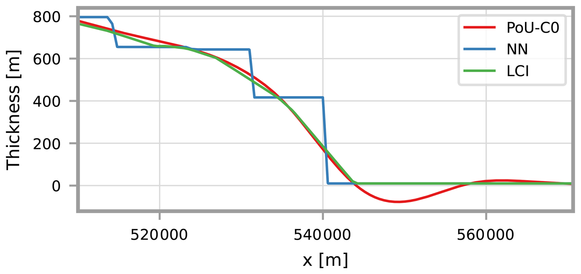
Figure 16 Results of mapping ice thickness from ISSM to CUAS mesh in the Greenland setup using different mapping methods along a horizontal section that crosses the ice boundary at $y=-\mathrm{1}\mathrm{277}\mathrm{863.4}$ m. Partition-of-unity radial basis functions (PoU-C0) overshoots and produces unphysical values at the ice boundary. Linear cell interpolation (LCI) is equivalent to the P1 finite elements used by ISSM. Nearest neighbor (NN) is constant in regions around ISSM vertices.

Figure 17 shows the total runtime required to initialize preCICE for both participants. This time includes both communication, mesh partitioning, and initializing data mappings. For all methods, initialization of preCICE is around the same order as initialization of the solvers (see Figs. 10 and 11). LCI is about twice as expensive as PoU and almost four times as expensive as NN.

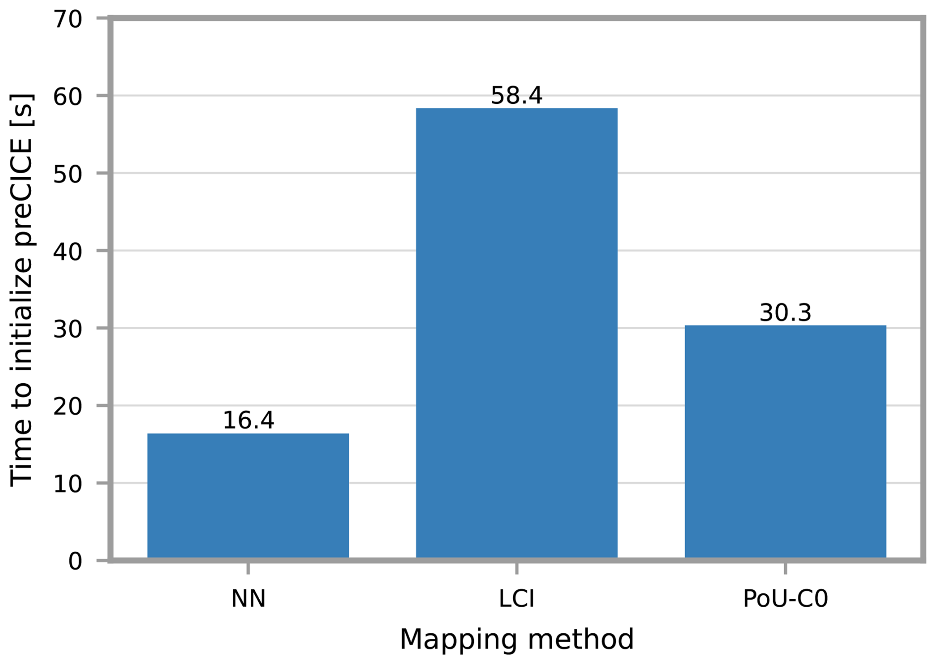
Figure 17 Time required to initialize preCICE for both coupling participants in the Greenland setup for different mapping methods: nearest neighbor (NN), linear cell interpolation (LCI) and partition-of-unity radial basis functions with C0 compact polynomial basis (PoU-C0). Both participants use the same mapping method, mapping is computed by the reading participant.

Figure 18 shows the runtime required to map the data in each coupling window. The cost difference between the mapping directions (ISSM to CUAS or CUAS to ISSM) can be attributed to the number of fields that must be mapped. NN and LCI are very close in cost, whereas PoU is significantly more expensive. However, for all mapping methods, the runtime of a coupling window (see Fig. 15) is dominated by the solvers themselves. NN was measured at approximately 9 ms from CUAS to ISSM, 25 ms from ISSM to CUAS, or ∼0.1 % and ∼0.3 % of the total time of a coupling window. LCI was measured only slightly slower, at 10 ms (∼0.1 %) and 29 ms (∼0.4 %). Note that the difference is too small to be reliably measured with this setup. The cost of PoU, on the other hand, is not as negligible, with 58 ms (∼0.7 %) and 380 ms (∼6 %). The detailed profile shows a significant imbalance in the distribution of work, probably due to the uneven mesh resolution. The slowest processes work up to four times longer than the fastest.

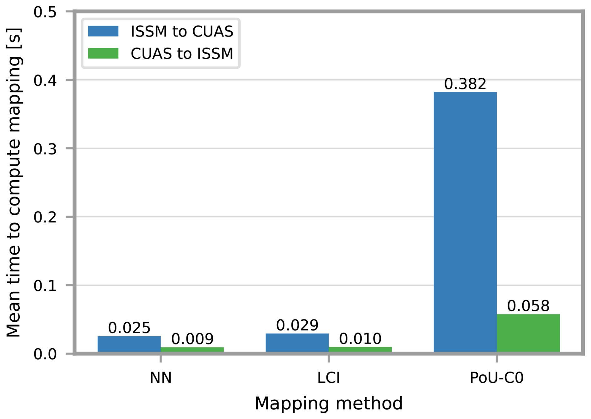
Figure 18 Time required to compute data mapping per coupling window in the Greenland setup for different mapping methods: nearest neighbor (NN), linear cell interpolation (LCI) and partition-of-unity radial basis functions with C0 compact polynomial basis (PoU-C0). Mapping is computed by the reading participant.

4 Discussion

The new coupling framework presented in this paper is a promising approach for the development of coupled ice sheet and Earth System Models. Compared to SHAKTI (Sommers et al., 2018), DoCo (de Fleurian et al., 2016), and other hydrology models directly integrated into ISSM, external coupling (with preCICE or another library, see discussion below) allows more choice of implementation and numerical treatment. Development of the models can progress independently, and neither model is restricted by the choices of the other. The effort to set up the coupling is minimal. Coupling scheme, data mapping, and coupling time window are easy to adapt and extend to additional participants.

The ISSM-preCICE adapter provides the basic features necessary for most use cases. It significantly reduces the effort required to couple other codes to ISSM, but it will almost certainly become necessary to allow the adapter to be customized more, e.g., to add logic specific to each coupling setup, such as deriving model variables as we already had to do in the CUAS adapter. Additionally, we listed some general limitations to be resolved in Sect. 2.3. For example, accuracy is lost because the coupling interface is based on the mesh vertices instead of finite element nodes, and it is not yet possible to couple the full three-dimensional volume of the ice sheet. Some features of ISSM and preCICE are not supported at this stage, among them dynamic adaptive meshes and time interpolation. It was not necessary to modify the code of ISSM to implement the adapter, but future extensions may require such changes.

The CUAS-preCICE adapter is an early prototype and does not yet follow most of the guidelines for preCICE adapters. Specific adaptations had to be made to CUAS to support the coupling with ISSM. These can be generalized to open the adapter for different use cases. In addition, the adapter needs to be cleanly integrated into the code, as CUAS-MPI itself aims for a high degree of software quality.

We have demonstrated the stability and functionality of the coupled system in Sect. 3.1. Within both 1-way and 2-way coupling, the fields for N, v_b, T_e and H are consistent, indicating that the hydrological system is well set up. Our results reveal that the differences between the physical fields in 1- and 2-way coupling are significantly larger with high seasonal forcing. The larger the runoff, the more important a multiphysics approach is. The more realistic feedback is found by using 2-way coupling, as the two systems adapt to a joint state with reasonable physical fields in both systems. The time series (Fig. 6) exemplifies that the winter state in the runoff forced case has a higher $\stackrel{\mathrm{‾}}{\log \left(T_{\mathrm{e}}\right)}$ in winter than without seasonal runoff, which is reasonable. The lower $\stackrel{\mathrm{‾}}{\log \left(T_{\mathrm{e}}\right)}$ in the 2-way coupling corresponds to lower $\stackrel{\mathrm{‾}}{N}$ in the high runoff forcing and vice versa, as N also influences the evolution of T_e. To summarize, the behavior of the ice and hydrology systems are reasonable, the simulated feedback is expected, but the drastic difference in 2-way coupling was not expected to this extent. As this paper focuses on the technical aspects of the coupling, we have not quantified the numerical accuracy of the coupled system nor fully demonstrated its ability to represent real-world cases. We have also not fully explored all preCICE features. In particular, informed choices need to be made regarding the optimal coupling scheme and the data mapping method.

Our performance experiments in Sect. 3.2 show that preCICE coupling does not negatively affect scaling during the simulation. Data mapping has negligible computational overhead, enabling coupling windows at least as short as the ISSM time step. preCICE time interpolation can be used in the future to improve temporal resolution if necessary, as shortening the ISSM time step would be expensive. Adaptive coupling windows would also be an option, but are not currently supported by preCICE.

Serial coupling is around 5 % faster than parallel coupling up to 1024 processes. There is tentative evidence that parallel coupling widens the range of CPU counts that can be used efficiently. On the other hand, an imbalance in the solver scaling limits the scaling of the coupled system. Reducing the imbalance by redistributing CPUs does not significantly improve overall execution times because it involves reassigning CPUs from well-scaling CUAS to worse-scaling ISSM. If there are many runs with the same number of CPUs and similar setups, it may be worth searching for the optimal distribution. Otherwise, an approximate solution is sufficient and probably uses fewer resources overall. It is also technically easier to allocate a distribution where every solver is assigned entire cluster nodes.

The cost of coupling and data mapping is higher during initialization than during the actual simulation. Partitioning the coupling mesh and computing the mapping weights takes about the same amount of time as initializing the solvers themselves. The required time depends on the chosen mapping method. Linear cell interpolation, a second order method, is twice as expensive as first-order nearest neighbor interpolation. The partition-of-unity method shows promising performance for second-order (or higher) mapping, particularly the initialization times, but algorithmic improvements and special handling of discontinuous fields (e.g., specially adapted meshes) are required for it to be suited for our setup.

Other researchers have reported (sometimes significantly) faster initialization times for other couplers for comparatively sized setups, for example YAC (Hanke et al., 2016; Hanke and Redler, 2019) or C-Coupler (Liu et al., 2023). As noted, we have not performed analysis of the initialization process internal to preCICE. Based on the profiles included in the supplement to this paper Abele et al. (2026) we believe that partitioning of the meshes, which in preCICE currently requires disk IO, is a contributor and could also be responsible for the slower initialization time of LCI over NN mapping.

The performance results give future users a basis for how to run the coupling efficiently. The relative solver and coupling execution times depend on too many factors (meshes, parameters, tolerances, etc.) to cover here. But estimates can be used to translate our results to other setups. Unlike the computation during simulation, initialization takes more time with added processes. Therefore, the length of the simulation, and with it the balance of initialization and simulation time, needs to be considered when choosing how to allocate resources.

preCICE has so far not been widely used in the Earth System Modeling community. While few (if any) ready-to-use adapters relevant to Earth System Modeling exist at the moment, developing such adapters is a current opportunity. Besides ESM-specific codes, models in frameworks like OpenFOAM, Elmer, or FEniCS/FEniCSx, for which preCICE adapters already exist, can be coupled with minimal effort. This makes these frameworks a good choice for the development of new models. For example, the ice sheet code Elmer/Ice could easily be coupled to CUAS-MPI using the adapters presented in this work. As mentioned in the introduction, Elmer/Ice already includes a different hydrology model, but being able to compare different approaches is highly valuable, as demonstrated by the various model intercomparison projects.

Without implementing comparable adapters for the same models, it is not possible to make a strong determination whether to prefer preCICE over a coupling library like YAC (Hanke et al., 2016) or OASIS3-MCT (Craig et al., 2017) that are specialized for Earth System Models. We found that preCICE works very well in our setup. The software is mature. Basic adapters can be developed quickly, but of course a generic adapter for a large model like ISSM still requires significant effort to build and maintain. The adapters that we presented here, as well as the other existing adapters, show that preCICE is compatible with various solver architectures. The features of preCICE (mapping methods, cartesian coordinates) are well-suited for our use case, and the library provides potentially beneficial features such as time interpolation (Rodenberg and Uekermann, 2025) that can be enabled in the future with extensions to the ISSM and CUAS adapters. The absence of features provided by ESM-specific couplers did not impede our implementation, but they remain highly relevant for other ESM applications. Further development is probably needed to satisfy the requirements of the community. Features that are required or at least desirable include spherical coordinate systems, specialized conservative mapping methods, masking, temporal accumulation such as in OASIS3-MCT (Craig et al., 2017), loading of mapping weight files, support for calendars, and others. Above, we also discussed issues in initialization performance that require further investigation and optimization. A comprehensive comparison of the numerical and computational performance of the mapping methods using identical meshes is also necessary. We think this effort is warranted due to the potentially much larger community that multidisciplinary cooperation in the development of coupling libraries and adapters brings.

5 Conclusions

In this paper, we presented the software for coupling the ice sheet model ISSM to the subglacial hydrology model CUAS-MPI. The main work has been to develop the adapters for the models for the coupling library preCICE. The ISSM adapter is generic and supports other use cases such as ice–ocean coupling, but adaptations will probably be necessary in some cases. The CUAS-MPI adapter is still a prototype and specific to coupling with ISSM. Future development will focus on generalizing the adapter and better integrating it into the CUAS-MPI code.

The coupling is easy to use, adaptable, and extensible due to the generic coupling library. We have demonstrated its functionality in a synthetic setup to verify its correctness and stability. We have also analyzed different aspects of the system's performance, including initialization times, scaling, and mapping methods. The system scales well with the number of processes, and the overhead for coupling is low. These experiments can inform the efficient use of the software in the future. Comparatively slow initialization performance is a concern that should be addressed in further development.

We were able to at least qualitatively compare preCICE to libraries specialized on Earth System Modeling. We found preCICE to be competitive in most aspects for our use case. However, in addition to the aforementioned performance issues, we have also identified some missing features that are required by other ESM applications. These are all possible future improvements for preCICE to better serve this community.

The new coupling will facilitate studies of the interaction between continental ice sheets and the hydrology systems underneath. We will also use the generic ISSM-preCICE adapter in other setups. For example, we are developing a new solver for capturing the ice sheet calving fronts that can be coupled with ISSM to improve upon its existing moving front core. The use of preCICE to integrate ISSM into a global Earth System Model will be evaluated. Finally, the adapters can be extended to lift some of the limitations described in this paper and open even more use cases.

We hope that the software we developed enables researchers to implement and test new ice sheet model capabilities more quickly. In general, researchers should consider preCICE coupling when developing new models or extending existing ones.