MIPV-NWP-PINNs V1.0: development of a multi-scale photovoltaic power forecasting framework integrating numerical weather prediction with physics-informed neural networks

Photovoltaic (PV) power generation has become a cornerstone of clean energy, for which accurate forecasting is essential to ensure safe and efficient grid integration. However, achieving reliable PV power forecasts remains challenging due to two primary sources of uncertainty: inherent errors in Numerical Weather Prediction (NWP)-derived meteorological variables, particularly solar irradiance, and the complex nonlinear conversion process from meteorological inputs to PV power output, which is influenced by both atmospheric conditions and PV module characteristics. To address this challenge, this study develops a multi-scale PV power forecasting framework that integrates NWP with deep learning techniques and evaluates its performance using PV module monitoring data from a power station in northwestern China. First, a regional high-resolution NWP system based on the Weather Research and Forecasting (WRF) model is established to generate multi-scale meteorological forecasts with lead times of 6 h, 1, 3, and 5 d. Next, a novel hybrid correction model that combines Quantile Mapping with a Temporal Pattern Attention-based Long Short-Term Memory (TPA-LSTM) network is proposed to improve the accuracy of Global Horizontal Irradiance (GHI) forecasts. This correction approach reduces the Mean Absolute Error (MAE) and Root Mean Squared Error (RMSE) by more than 23 % compared to raw NWP outputs. Building on these corrected meteorological forecasts, a Physics-Informed Neural Networks (PINNs)-iTransformer model is developed for the final PV power prediction. By incorporating physical constraints directly into its loss function, this model consistently outperforms state-of-the-art alternatives across all forecasting horizons, achieving reductions of 15.5 % in RMSE and 12.4 % in MAE. This physics-constrained framework substantially improves the accuracy and robustness of PV power forecasting across multiple time scales. The enhanced reliability directly supports secure PV grid integration and contributes to the broader transition toward low-carbon energy systems.

1 Introduction

The rapid expansion of Photovoltaic (PV) power is reshaping the global energy landscape; it is projected to become the dominant renewable energy source by 2029 and is expected to constitute 8.3 % of the total electricity supply by 2025 (IEA, 2024). In this context, Northwest China, with its abundant solar resources, has become a key region for the global PV industry's growth. The region's high solar irradiance and clear-sky index provide ideal conditions for large-scale, centralized PV plants, establishing it as the primary area for such deployments in China. However, the challenge of accurate PV forecasting is magnified in this region, which is characterized by an arid desert climate and complex meteorological dynamics. This environment is not only susceptible to frequent extreme weather, such as dust storms, but also experiences significant attenuation and variability in Global Horizontal Irradiance (GHI) due to high concentrations of anthropogenic aerosols (Nie and Mao, 2021). These uncertainties impair PV module performance and threaten power grid stability. Consequently, accurate PV power prediction is essential for ensuring the economic viability of power stations and maintaining system stability.

The first key challenge lies in the limited accuracy of NWP-derived GHI. High-precision meteorological forecasts are crucial for PV power prediction, yet many studies inflate model performance by using actual weather data as input, which does not reflect real-world forecasting scenarios (Das et al., 2018; Dai et al., 2025). While Numerical Weather Prediction (NWP) provides operational forecasts, its outputs often exhibit significant deviations from observations. Mainstream radiation transfer schemes, such as those in the Weather Research and Forecasting (WRF) model, systematically overestimate GHI, and this bias is amplified by increasing cloud cover and aerosol influence (Zempila et al., 2016; Yue et al., 2025). Although incorporating aerosol factors can mitigate this (Ruiz-Arias et al., 2014), the inherent deficiencies in representing cloud microphysics often lead to persistent biases. Given the complexity of directly modifying NWP model cores, statistical post-processing techniques have emerged as cost-effective alternatives. Kalman filtering reduced WRF-generated GHI RMSE by 17 % (Visaga et al., 2024), and nonlinear regression models have been employed for bias correction (Khan and Jama, 2024). A combined Kalman filter with model output statistics achieved up to 97 % reduction in annual GHI bias (Rincón et al., 2018). Furthermore, Artificial Neural Network (ANN)-KF hybrid models reduced raw GHI MAE by 45 % (Alvarenga et al., 2022). These studies demonstrate that statistical post-processing is a powerful tool for improving NWP forecast accuracy at a modest computational cost. Despite these advances, opportunities remain for developing more sophisticated correction algorithms to further improve forecast reliability.

The second challenge concerns the “black-box” nature and lack of physical consistency in data-driven PV power forecasting models. Converting meteorological forecasts into PV power predictions requires a subsequent modeling step, and existing methods are broadly classified into physical, data-driven, and hybrid models (Gupta et al., 2025; Li et al., 2025). Physical models, such as the five-parameter model (De Soto et al., 2006), simulate power output based on PV module characteristics but often show limited practical performance (Wang et al., 2019). Data-driven methods, including traditional machine learning (Alskaif et al., 2020; Kumar et al., 2025) and deep learning architectures such as Long Short-Term Memory (LSTM) (Guo et al., 2025; Liu et al., 2024) and Transformer (Piantadosi et al., 2024; Wu et al., 2024a), have become mainstream due to their flexibility and accuracy. However, these purely data-driven models lack physical interpretability and may yield outputs that violate fundamental physical laws, particularly when training data are sparse or noisy.

Physics-Informed Neural Networks (PINNs) offer a promising solution to address these limitations. Hybrid models that fuse physical principles with statistical learning have emerged to improve PV power forecasting, ranging from mechanism-driven hybrids to statistical-physical fusion models (de Oliveira Santos et al., 2024). A common strategy involves a “shallow” or sequential integration of physics. For instance, the Physical-Hybrid Artificial Neural Network (PHANN) couples a solar radiation model with MLP (Dolara et al., 2015; Hottel, 1976). Other works have used physical models to compute module-surface irradiance as input features for LSTM networks (Wu et al., 2024b), or to establish a baseline physics prediction that an ANN subsequently refines to capture residual dynamics (Zhang et al., 2024). However, these cascaded frameworks lack deep mechanistic integration. In contrast, PINNs embed physical laws directly into the loss function, compelling the model to adhere to physical principles during training (Raissi et al., 2019). Although PINNs have been applied to related PV tasks, such as temperature prediction (Wang et al., 2025), their direct application to PV power forecasting remains underexplored. Deeply coupling PINNs with advanced time-series models for direct PV power prediction is a significant yet largely untapped research area with substantial scientific merit.

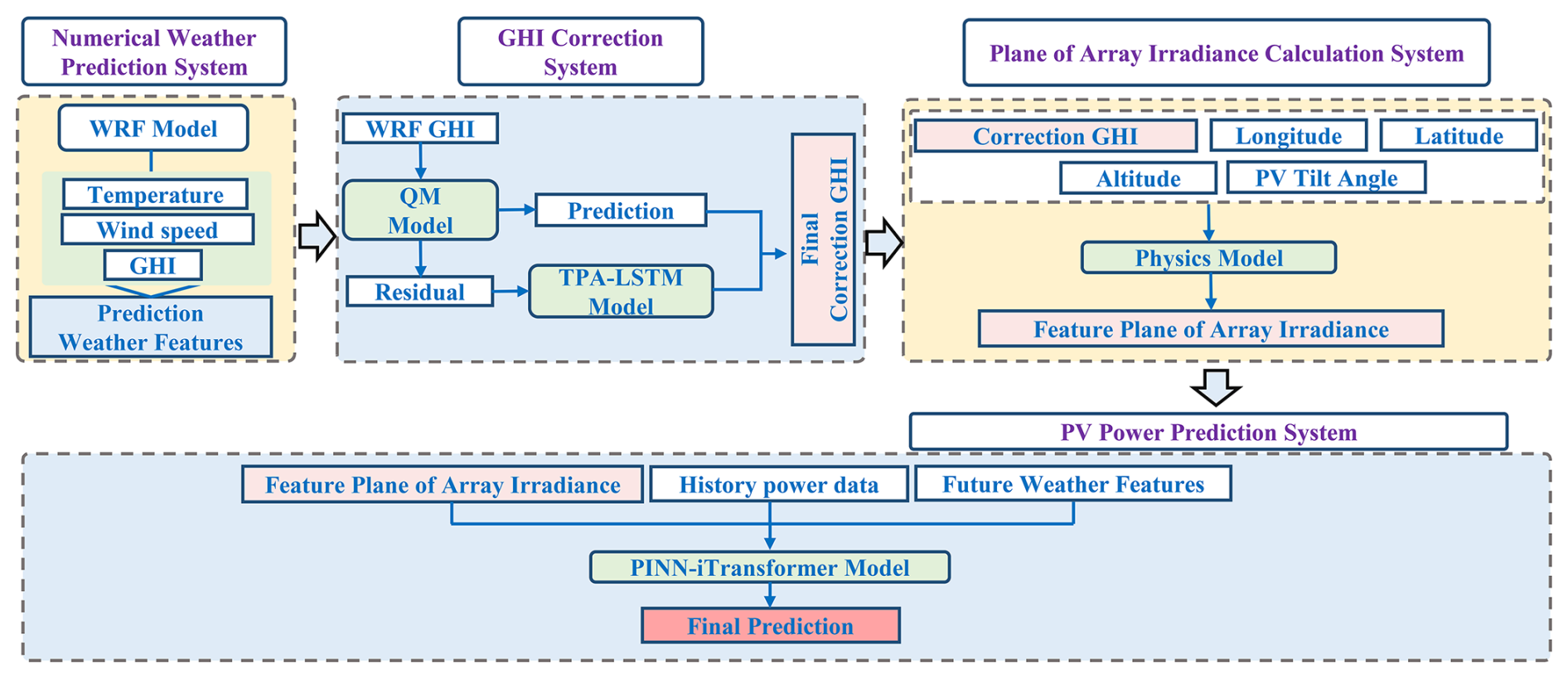
To bridge these research gaps, this study develops an NWP-driven multi-scale photovoltaic forecasting framework that fundamentally integrates physical principles with data-driven modeling through deep synergistic coupling. The framework comprises a hierarchical, multi-module forecasting chain, with its technical pipeline illustrated in Fig. 1. Firstly, we establish a WRF prediction system to generate fine-grained numerical weather forecasts. Secondly, we design a hybrid correction module employing a Quantile Mapping-Temporal Pattern Attention-Long Short-Term Memory (QM-TPA-LSTM) network to enhance the GHI accuracy. Following this, a physical model is utilized to calculate the plane-of-array irradiance (G_POA). For the final task of PV power prediction, we construct a PINNs-iTransformer model by incorporating the physical equations constraint. This “physics-constrained, data-driven” hybrid architecture excels in statistical performance and significantly improves physical consistency and interpretability. This paper is structured as follows: Sect. 1 provides an introduction to the study's core issues and scope. Section 2 presents the theoretical underpinnings and methodologies employed. Section 3 elaborates on the process of GHI correction and estimation. Section 4 details the PV power prediction, including a comparative analysis against other established models. Finally, Sect. 5 discusses the key factors and uncertainties in forecasting.

Figure 1 Flowchart of the PV power forecasting framework.

2 Data and Methods

2.1 Data Acquisition

The proposed forecasting framework was empirically evaluated using high-resolution data from a PV power station in Zhongwei, Ningxia, China (37.53° N, 105.04° E), as depicted in Fig. 2c. The system recorded key variables including ambient air temperature, GHI, wind speed, wind direction, PV module temperature, and PV power output. Data were collected from 1 June to 31 July 2020, with a temporal resolution of 120 s. This observational dataset was used to calibrate and evaluate all NWP simulations and subsequent power forecasting models. The technical specifications and related parameters of the sampling equipment are detailed in Table S1 in the Supplement. We incorporated GHI data from six additional National Solar Radiation Database (NSRDB) stations to assess the framework's spatial generalizability. The GHI data from these stations are well-established to exhibit high agreement with ground-based measurements (Sengupta et al., 2018). The geographical distribution of these six stations is illustrated in Fig. 2b.

2.2 The WRF Numerical Model

High-resolution regional meteorological forecasts were generated using the WRF model (version 4.1) (Stossmeister et al., 2019). A four-level nested domain configuration was employed with horizontal resolutions of 27, 9, 3, and 1 km for domains d01 to d04, respectively, as illustrated in Fig. 2a. This progressively refined grid setup enables downscaling large-scale weather patterns to a kilometer-scale resolution.

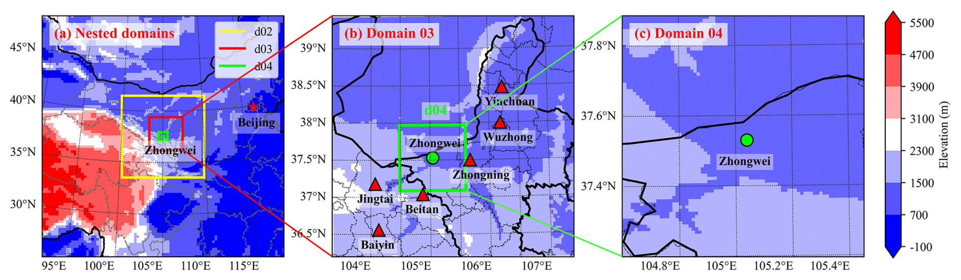
Figure 2 WRF model domain configuration and site locations. (a), Topography of the four nested WRF domains (d01–d04). (b), Map of a subregion within the d03 domain, where red markers indicate the locations of the evaluation sites. (c), A zoomed-in map of the d04 domain, with the green point marking the location of the primary observation station.

The WRF simulation period covered from 00:00 UTC on 1 June 2020, to 23:00 UTC on 31 July 2020, with hourly outputs. To emulate a realistic operational forecasting procedure, we implemented a rolling forecast scheme to create forecasts with horizons of 6, 24, 72, and 120 h. In the WRF model, the atmospheric state at the initial time is typically imbalanced. The “spin-up” period is employed to allow the model's internal physical variables (such as soil moisture and cloud microphysics) to reach thermodynamic equilibrium. If this period is not discarded, the pronounced fluctuations present at the beginning may contaminate the subsequent weather prediction results (Mallard et al., 2026). The initial 12 h of each simulation run were discarded as a spin-up period to ensure forecast accuracy. Consequently, the actual simulation duration was set to N+ 12 h to obtain a valid N-hour forecast. Specifically, estimates of 6, 24, 72, and 120 h corresponded to simulation durations of 18, 36, 84, and 132 h, respectively. Each forecast cycle was initialized and bounded by the Final Operational Global Analysis data from the National Centers for Environmental Prediction (Contributor, 2015), and data assimilation was turned off across all domains. This approach not only simulates real-world forecasting practices but also reduces initial condition errors. Table S2 presents the central physics parameterization schemes used in this study. The Dudhia scheme (Dudhia, 1989), a widely adopted model in the field, was employed for shortwave radiation.

2.3 QM-TPA-LSTM Radiation Correction Model

This study proposes QM-TPA-LSTM, a hybrid post-processing model designed to correct inherent biases in NWP forecasts. The model employs a two-stage sequential correction strategy to perform rolling corrections on the GHI output from the WRF model, as illustrated in Fig. 1. The QM method provides an initial statistical bias correction in the first stage. In the second stage, a TPA-LSTM network models and predicts the residual errors from the first stage. The final, refined GHI forecast is then obtained by aggregating the corrected GHI with the TPA-LSTM-predicted residuals.

QM is a highly reliable statistical method for climate bias correction (Sun et al., 2022). It performs corrections based on the statistical distributions of data rather than complex physical processes. For example, studies have shown that QM reduced WRF-simulated rainfall RMSE by 34 % (Charoensuk et al., 2024), effectively minimized errors in soil moisture predictions (Koujani et al., 2025), and significantly improved precipitation and temperature forecasts (Ngai et al., 2017). The fundamental principle of QM is that for a given raw WRF forecast value, its quantile in the distribution of the raw WRF training data should be identical to the quantile of the corrected value in the distribution of the observed training data (Charoensuk et al., 2024). In this study, we employ the empirical cumulative distribution function. Although the QM correction enhances forecast accuracy, the residual errors contain valuable, yet uncaptured, predictive information. The TPA-LSTM network is employed to capture these dynamics. The TPA mechanism enhances the standard LSTM by using the final hidden state as a query to compute attention weights over all previous hidden states. A context vector is then formed as a weighted sum, allowing the model to selectively focus on historically relevant features for the current prediction, thereby improving forecast accuracy (Shih et al., 2019).

2.4 Calculation of Irradiance on the PV Module Surface

Although GHI can directly influence the power conversion efficiency of PV modules and is therefore widely used in PV power forecasting, GHI does not represent the actual irradiance incident on and absorbed by the module surface. In contrast, the G_POA, which characterizes the irradiance received by the PV module surface, can more accurately capture variations in PV power generation. As shown in Fig. 3a, the instantaneous position of the sun is defined by key geometric parameters, including the solar zenith angle, solar azimuth angle, and solar elevation angle. These angles exhibit periodic, dynamic changes over time, leading to significant variations in the solar irradiance received by the PV module at different times. This variation follows a well-defined astronomical time function. Figure 3b further elucidates the physical composition of the irradiance received on the module surface. This total irradiance is a superposition of three components: the projection of Direct Normal Irradiance (DNI) onto the module plane, Diffuse Horizontal Irradiance (DHI), and ground-reflected irradiance (Mahmoudi et al., 2024; Anderson et al., 2023). Accurate calculation of G_POA requires the decomposition of GHI and the application of a radiation transposition model that incorporates the module's tilt and azimuth angles. This is a critical step toward achieving high-precision PV power forecasting. The underlying physical principles are as follows:

$$\begin{array}{}\text{(1)}& G_{\mathrm{POA}}=G_{\mathrm{b}}+G_{\mathrm{g}}+G_{\mathrm{d}}\end{array}$$

Here, G_POA represents the total solar irradiance on the PV module surface, G_b denotes the beam irradiance on the tilted plane, G_g is the isotropic ground-reflected irradiance, and G_d signifies the diffuse sky irradiance. The beam irradiance is calculated as:

$$\begin{array}{}\text{(2)}& G_{\mathrm{b}}=\mathrm{DNI}\cdot \cos {\mathit{\theta }}_{\mathrm{i}}\end{array}$$

where θ_i is the angle between the sun's rays and the normal to the photovoltaic module surface (the angle of incidence). This angle can be expressed by the following equation:

$$\begin{array}{}\text{(3)}& \begin{array}{rl}\cos {\mathit{\theta }}_{\mathrm{i}}& =\sin \mathit{\phi }\cdot \sin \mathit{\delta }\cdot \cos \mathit{\beta }-\cos \mathit{\phi }\cdot \cos \mathit{\gamma }+\cos \mathit{\phi }\cdot \cos \mathit{\delta }\\ & \cdot \cos \mathit{\omega }\cdot \cos \mathit{\beta }\end{array}\end{array}$$

Here, φ is the latitude of the module's location, δ is the solar declination angle, γ is the azimuth angle of the PV module, ω is the hour angle, and β is the tilt angle of the PV module installation.

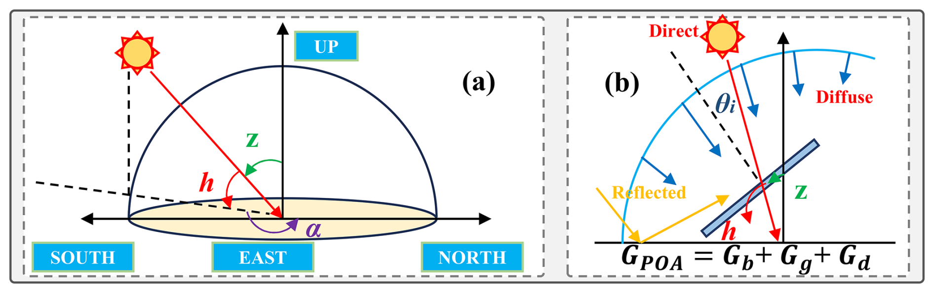
Figure 3 Solar geometry and irradiance components. (a), Schematic illustrating the solar zenith, azimuth, and altitude angles. (b), Components of solar irradiance on a tilted PV module surface.

The calculation principle for G_g is as follows:

$$\begin{array}{}\text{(4)}& G_{\mathrm{g}}=\mathrm{GHI}\cdot \mathit{\rho }\cdot {\displaystyle \frac{\left(\mathrm{1}-\cos \mathit{\beta }\right)}{\mathrm{2}}}\end{array}$$

The calculation principle for G_d is as follows:

$$\begin{array}{}\text{(5)}& G_{\mathrm{d}}=\mathrm{DHI}\cdot R_{\mathrm{d}}\end{array}$$

where R_d is the diffuse transposition factor.

Model for calculating G_POA are integrated into the pvlib-python library developed by Sandia National Laboratories (Anderson et al., 2023). In this study, we first employed the Erbs model to decompose GHI (Erbs et al., 1982). Subsequently, the classic Hay-Davies anisotropic sky model was used to calculate the diffuse irradiance received on the tilted surface of the PV module (Hay, 1979). The ground-reflected irradiance component was estimated based on a constant ground albedo of 0.2, a typical value for common vegetation or soil surfaces. We calculate the G_POA of the PV panel. A comparison between the corrected GHI and the derived G_POA is presented in Fig. S1a. While the GHI generally exhibits a strong temporal correlation with the G_POA, significant deviations reaching magnitudes of up to 200 W m⁻² (Fig. S1b). These discrepancies underscore the necessity of explicitly computing rather than utilizing GHI as a direct proxy.

2.5 PINNs-iTransformer Framework

We developed the PINNs-iTransformer model to achieve high-precision, multi-scale PV power forecasting by integrating physical mechanisms with an advanced deep learning architecture. This module utilizes iTransformer as its backbone network to capture complex temporal dependencies, while embedding constraints from a semi-empirical physical model via the PINNs framework to enhance its generalization capability and physical interpretability.

2.5.1 iTransformer Model

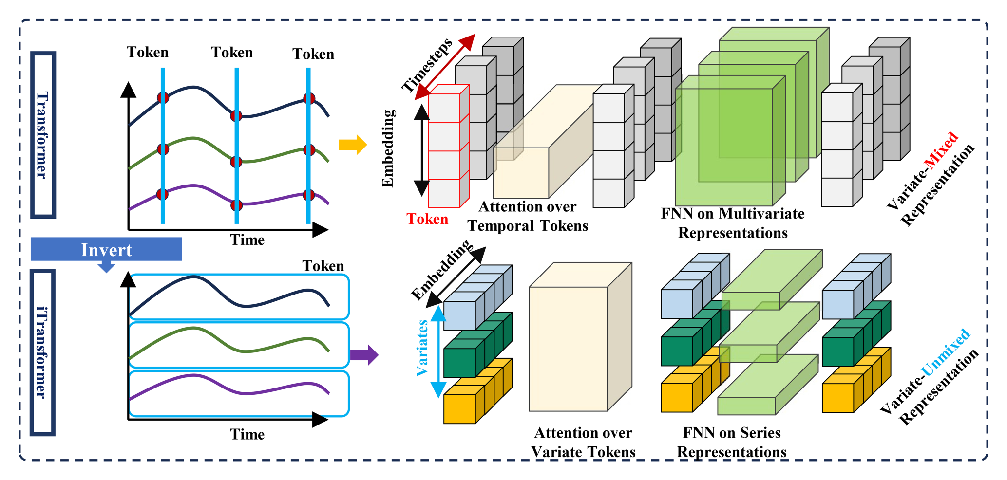
Transformer-based architectures are widely used in time series forecasting for their ability to capture complex temporal patterns (Piantadosi et al., 2024; Wu et al., 2024a). However, when processing multivariate time series, the conventional Transformer embeds data points from the same time step but different variables into a single token, which can weaken the correlations between variables. As shown in Fig. 4, iTransformer inverts the roles of the feed-forward network and the attention mechanism within the Transformer framework. Specifically, it embeds the time points of individual series into variable-tokens, which are then processed by the attention mechanism to capture inter-variable correlations (Liu et al., 2023).

Figure 4 Schematic of the modified iTransformer architecture.

2.5.2 Physics-Informed Neural Networks

• a.

  Semi-empirical Physical Model. To integrate a priori physical knowledge into our data-driven framework, we employ a semi-empirical PV power model as a physical constraint. This model class was chosen for its ability to balance model complexity and predictive utility effectively. The study employs the efficient semi-empirical model proposed by Fan et al. (2025), which estimates power output based solely on solar irradiance, ambient temperature, wind speed, and a coefficient that represents the module's thermal loss characteristics. Its advantages lie in its minimal parameter requirements and high computational efficiency while retaining a description of the core physical processes.

  $$\begin{array}{}\text{(6)}& {\displaystyle }{P}_{\mathrm{phy}}=f_{\mathrm{PV}}\left({\displaystyle \frac{G_{\mathrm{POA}}}{G_{\mathrm{STC}}}}\right)\left[\mathrm{1}+{\mathit{\alpha }}_{\mathrm{PV}}\left(T_{\mathrm{c}}-T_{\mathrm{ref}}\right)\right]P_{\mathrm{MPP}}\text{(7)}& {\displaystyle }{T}_{\mathrm{c}}=T_{\mathrm{a}}+G_{\mathrm{POA}}\exp a+b\cdot {\mathit{\omega }}_{\mathrm{s}}\end{array}$$

  Where, P_phy is the PV power output, f_PV represents the photovoltaic module efficiency coefficient, which is intrinsically linked to the module's manufacturing process. G_STC is the irradiance on the module surface under standard test conditions, α_PV is the photovoltaic module temperature loss coefficient, T_c is the module temperature, and T_ref is the module temperature under reference conditions. P_MPP signifies the module's maximum power, ω_s represents the wind speed, and T_a denotes the ambient temperature. The coefficients a, b are undetermined parameters that can be fitted from historical data using the least-squares method.

• b.

  PINNs Model. To constrain the neural network predictions toward physically consistent solutions, we introduce a physics-informed regularization term based on a first-order relaxation ODE framework. Unlike empirical curve-fitting, this ODE serves as a mathematical regulator that quantifies the deviation of the neural network's predictions from the idealized physical equilibrium state. By penalizing the rate of divergence from physical bounds, the framework enforces a relaxation mechanism, ensuring that the model's outputs remain dynamically consistent with the underlying physical laws of PV conversion.

  The governing equation takes the form:

  $$\begin{array}{}\text{(8)}& {\displaystyle \frac{\mathrm{d}\widehat{P}\left(t\right)}{\mathrm{d}t}}=-k\cdot \left(\widehat{P}\left(t\right)-P_{\mathrm{eq}}\left(t\right)\right)\end{array}$$

  where $\widehat{P}\left(t\right)$ is the predicted power output, P_eq(t) is the equilibrium power derived from the semi-empirical photovoltaic performance model (Eqs. 6 and 9), and k is a learnable relaxation coefficient. The equilibrium power P_eq represents the theoretical steady-state output determined by instantaneous meteorological conditions:

  $$\begin{array}{}\text{(9)}& P_{\mathrm{eq}}\left(t\right)=P_{\mathrm{phy}}\left(t\right)\end{array}$$

  The physical interpretation of Eq. (8) is as follows: when the predicted power deviates from the equilibrium value, the equation enforces a tendency to restore consistency. The relaxation coefficient k governs the strength of this coupling-larger values impose stricter adherence to the physical model, while smaller values allow greater flexibility for data-driven corrections. Importantly, k is treated as a learnable parameter, jointly optimized with the network weights, enabling the model to automatically determine the appropriate balance between data fitting and physical consistency.

  For numerical implementation, the ODE is discretized using a forward difference scheme, and the physical residual is defined as:

  $$\begin{array}{}\text{(10)}& R\left(t\right)={\displaystyle \frac{\mathrm{d}\widehat{P}\left(t\right)}{\mathrm{d}t}}+k\cdot \left(\widehat{P}\left(t\right)-P_{\mathrm{eq}}\left(t\right)\right)\end{array}$$

  where $\widehat{P}\left(t\right)$ and P_eq(t) denote midpoint values for improved numerical accuracy. The physics-informed loss is computed as the normalized mean squared residual over daytime periods (when P_eq(t)>0):

  $$\begin{array}{}\text{(11)}& L_{\mathrm{pinn}}={\displaystyle \frac{\mathrm{1}}{N}}{\sum }_{i=\mathrm{1}}^N(R_i{)}^{\mathrm{2}}\end{array}$$

  The total loss function combines the data-driven and physics-informed components:

  $$\begin{array}{}\text{(12)}& L=L_{\mathrm{primary}}+\mathit{\lambda }{L}_{\mathrm{pinn}}\end{array}$$

  where λ is a weighting hyperparameter that balances the contribution of data fitting and physical consistency. During model optimization, this physics-inspired regularization term compels the network to converge towards a solution space that adheres to physical laws while fitting the observational data.

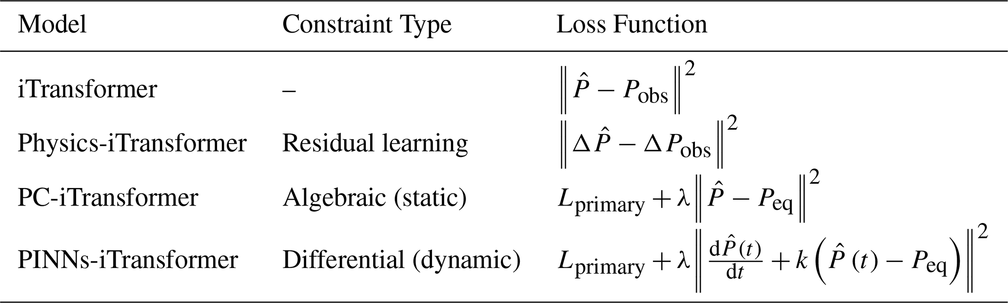
2.5.3 Comparative Model Frameworks

To rigorously evaluate the performance of the proposed PINNs-iTransformer, we benchmark it against three baseline configurations: the standard iTransformer, the Physics-iTransformer (a cascaded residual learning model), and the PC-iTransformer (a physics-constrained model). The structural and functional distinctions of the latter two physics-informed variants are detailed below:

• a.

  Physics-iTransformer (Cascaded Residual Framework). The Physics-iTransformer adopts a sequential two-stage hybrid architecture that explicitly separates the deterministic physical component from stochastic deviations. In the first stage, the theoretical PV power output P_phy is calculated by Eq. (6). In the second stage, an iTransformer is trained to predict the residual term ΔP, defined as the difference between the observed power and the physical estimate: $\mathrm{\Delta }P=P_{\mathrm{obs}}-P_{\mathrm{phy}}$. The final forecast, $\widehat{P}$ is obtained by superimposing the physics-based baseline with the data-driven residual correction: $\widehat{P}=P_{\mathrm{phy}}+\mathrm{\Delta }P$.

• b.

  PC-iTransformer (Physics-Constrained iTransformer). The PC-iTransformer preserves the core architecture of the standard iTransformer while incorporating physical consistency via a soft-constraint term in the training objective. Following the governing formulation of Fan et al. (2025), they introduce a physics-regularized loss component that penalizes deviations from the theoretical steady-state equilibrium. The overall loss is defined as:

  $$\begin{array}{}\text{(13)}& L=L_{\mathrm{primary}}+\mathit{\lambda }{L}_{\mathrm{PC}}\end{array}$$

  where λ represents the weighting coefficient for the physical constraint. The physics-constrained term is formulated as:

  $$\begin{array}{}\text{(14)}& L_{\mathrm{PC}}={∥\widehat{P}-P_{\mathrm{eq}}∥}^{\mathrm{2}}\end{array}$$

  which encourages the predicted power $\widehat{P}$ to remain close to the equilibrium power P_eq. Here, P_eq is computed from the physical relationship given in Eq. (9).

Table 1 The architectural differences, input configurations, and physical integration strategies across all compared models.

2.6 Error Evaluation Metrics

To quantify the predictive accuracy of the models, this study employs two widely recognized error metrics: the RMSE and the MAE. RMSE is particularly sensitive to large errors, effectively penalizing significant deviations or inaccuracies in peak prediction. In contrast, MAE provides a more straightforward measure of the average magnitude of prediction errors, reflecting the overall level of predictive performance (Jannah et al., 2024). The prevalence of these metrics in the field is underscored by a comprehensive review (Al-Dahidi et al., 2024; Pandžiæ and Capuder, 2024), which indicates that over half of the surveyed literature utilizes both RMSE and MAE for model evaluation.

3 Data Preprocessing and Feature Engineering

3.1 Reliability Analysis of NWP Output

Figure 5 presents a comprehensive evaluation of the WRF model against station observations, depicting scatter plots for temperature and GHI across varying lead times (6 h to 5 d) alongside GHI time-series comparisons. The WRF model exhibits high predictive skill for temperature across all lead times, demonstrating a strong correlation with observations and low error metrics. For GHI, the model accurately reproduces the diurnal cycle and overall trends and notably, effectively captures sharp declines in irradiance associated with sudden weather events, such as changes in cloud cover and precipitation (indicated by the light-red shaded area). This capability to represent the influence of key meteorological processes on solar radiation underscores the scientific merit of the WRF forecasts. Nevertheless, a persistent systematic overestimation bias is evident in the GHI forecasts, with maximum errors reaching an RMSE of 231.5 W m⁻² and an MAE of 159.3 W m⁻². As solar radiation is a direct input for photovoltaic power forecasting, this bias propagates directly into power predictions, introducing significant uncertainty. Consequently, bias correction of the model's radiation output is an essential step for subsequent applications (Lindsay et al., 2020).

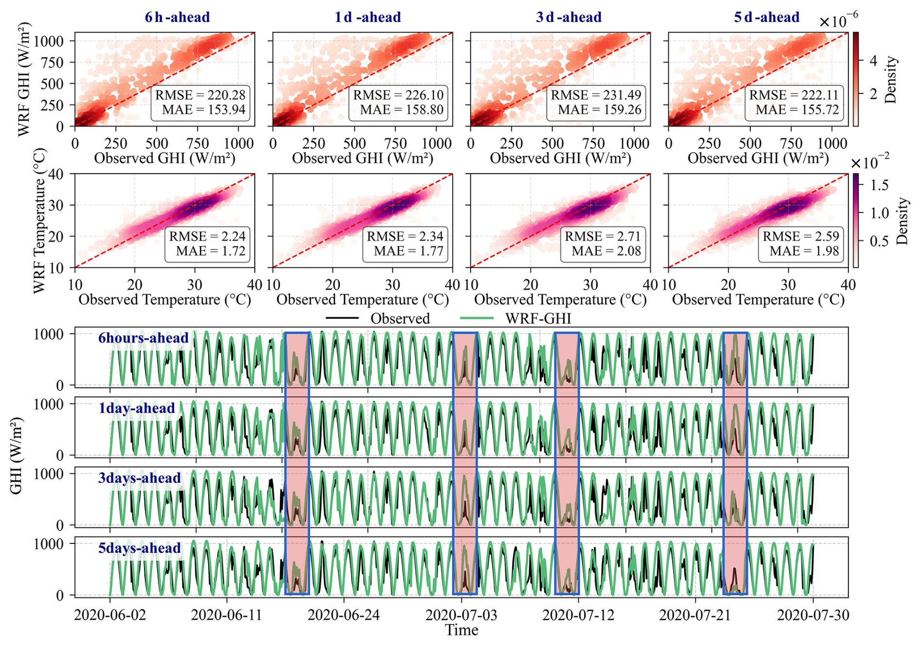
Figure 5 Comparison of WRF-simulated and observed meteorological variables at Zhongwei station (top scatter plots) and time series of observed GHI versus NWP predictions at various forecast horizons (bottom panels).

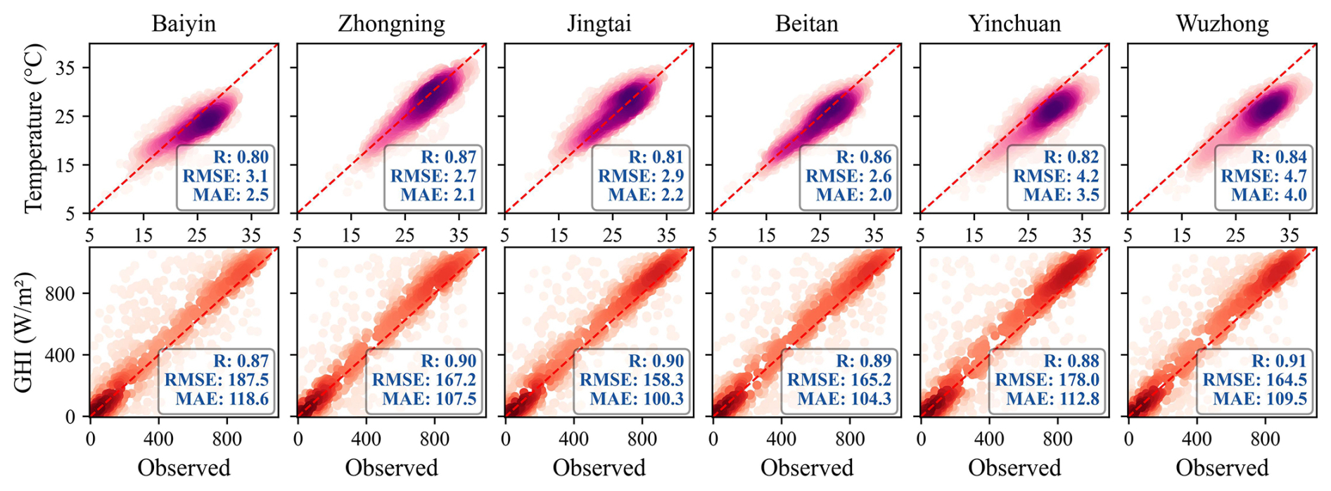
We cross-validated the WRF model's forecasts against data from six diverse reference sites (Fig. 2b) to rigorously assess its spatial generalizability. As illustrated in Fig. 6, the WRF model's performance at these external sites is highly consistent with its performance at the local observation station, with high correlation coefficients (R). While the GHI overestimation bias persisted, its magnitude was lower than at the primary Zhongwei site. A scale mismatch likely explains this reduction. The WRF simulation's 1 km × 1 km resolution at Zhongwei produces area-averaged irradiance, amplifying apparent GHI error compared to single ground-station point measurements. Conversely, the gridded NSRDB data provides better spatial representativeness and more closely matches the WRF output. This multi-site validation confirms that the WRF numerical model is reliable for short- to medium-range weather forecasting, providing robust environmental variable inputs for the subsequent PV power forecasting model.

Figure 6 Evaluation of meteorological forecasts at different sites.

3.2 GHI Correction

This study implements real-time, multi-step rolling corrections for the WRF-derived GHI, as illustrated in the forecasting scheme presented in Fig. 7. The framework leverages historical GHI observations and WRF meteorological parameters as inputs.

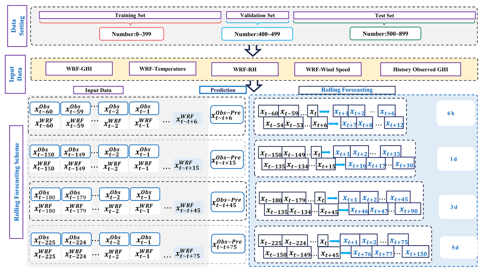
Figure 7 Schematic of the forecast output strategy. The forecast horizons are 6, 15, 45, and 75 steps, corresponding to lead times of 6 h, 1, 3, and 5 d, respectively.

During the data preprocessing phase, a dataset comprising 900 h of valid GHI observations was constructed after cleaning and filtering. This dataset covers 60 d, with 15 daytime hours selected from each day. The dataset was chronologically partitioned into three consecutive phases: a training phase (the first 400 steps), a validation phase (the subsequent 100 steps), and a test phase (the final 400 steps). It is important to note that these partitions represent temporal spans rather than static data splits; the rolling prediction mechanism described below ensures that all test-phase data are fully utilized for evaluation.

To simulate a realistic operational forecasting scenario, the forecast horizons were set to 6, 15 (one day ahead), 45 (three days ahead), and 75 (five days ahead) steps, aligning with the WRF rolling forecast mechanism. Correspondingly, the model used historical data from 60, 90, 180, and 225 steps as input, respectively. This input-output length configuration is designed to capture dynamic dependencies across different time scales.

The model's prediction process is realized through an automated, non-overlapping rolling-window mechanism, which operates as follows: (1) for a given forecast horizon of H steps, the model uses the preceding L steps of historical data to generate H-step-ahead GHI predictions; (2) after this prediction sequence is recorded, the prediction window advances forward by exactly H steps; (3) the model then generates predictions for the next H steps using the updated historical window; (4) this process iterates until the entire test phase (400 steps) is covered by consecutive, non-overlapping predictions. This rolling approach maintains strict temporal causality, ensuring that only historically available information is used for each prediction, thereby faithfully simulating operational forecasting conditions. Throughout this process, all 400 steps in the test phase are predicted and evaluated, with no data discarded. The efficacy of the GHI correction at the primary Zhongwei site is illustrated in Fig. 8. Its performance relative to benchmark models is detailed in Fig. 9, and the generalizability of the correction is demonstrated across six additional sites in Fig. 10.

Figure 8 Performance evaluation of the GHI correction model.

Figure 9 Comparison of different correction models for WRF-simulated GHI.

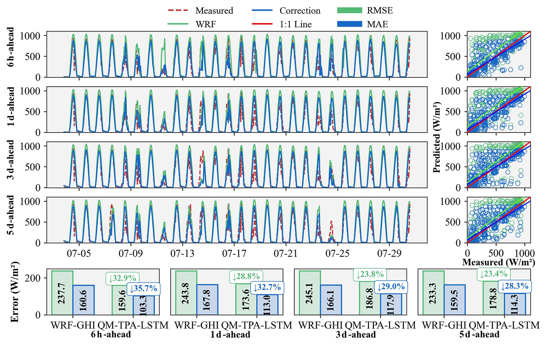
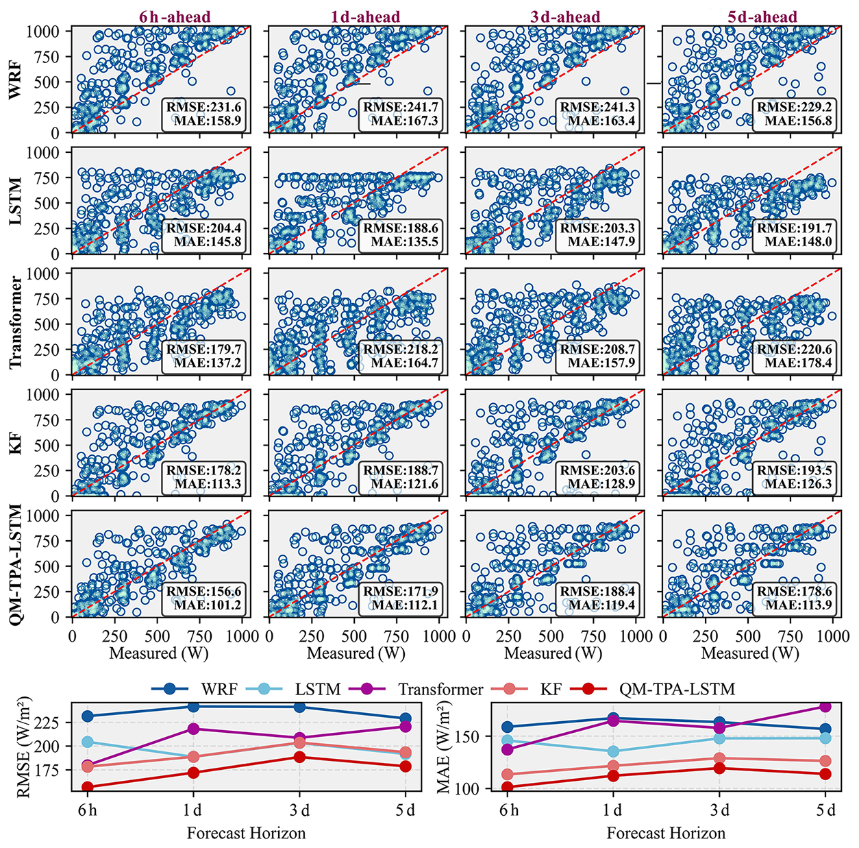
Figure 8 systematically illustrates the correction effect of the hybrid QM-TPA-LSTM model on the raw GHI forecasts at the Zhongwei site. The time-series plot (top) shows that the corrected GHI (blue) closely tracks the ground-truth measurements (red), effectively mitigating the substantial overestimation bias of the raw WRF forecast (green). The scatter plots on the right further corroborate this improvement from a statistical distribution perspective: the corrected data points (blue) converge more tightly around the 1:1 line (red), indicating a substantial improvement in the consistency between predicted and observed values. The bar charts at the bottom provide quantitative evaluations of RMSE and MAE across different forecast horizons. The results show that the corrected GHI exhibits a marked decrease in both RMSE and MAE under all conditions, with an average reduction exceeding 23 %, thereby significantly improving the quality of the GHI output.

The 6-step forecast horizon (6 h lead time) yielded optimal correction performance, with reductions in RMSE and MAE of 33 % and 36 %, respectively. However, correction performance declined as the forecast horizon was extended to 75 steps (a 5 d lead time). This degradation is attributable to: (1) the inherent difficulty of LSTM networks in maintaining effective memory over extended sequences (Hochreiter and Schmidhuber, 1997), as the 225-step historical input required for 75-step predictions approaches practical memory limits; (2) the chaotic nature of atmospheric dynamics, which causes forecast errors to accumulate nonlinearly with increasing lead time; and (3) the limited temporal coverage of the current dataset (60 d), which constrains the model's capacity to learn high-frequency meteorological fluctuations. Future work will address these limitations by expanding dataset coverage and incorporating explicit periodic encoding mechanisms.

The proposed QM-TPA-LSTM model was evaluated against three benchmarks across multiple forecast horizons: LSTM (Yang et al., 2025; Sun et al., 2022) and Transformer (Piantadosi et al., 2024; Wu et al., 2024a), as well as the KF model, which is widely used in meteorological correction (Visaga et al., 2024). As shown in Fig. 9, all models successfully corrected the raw WRF GHI output, demonstrating the efficacy of the post-processing framework. However, the classic KF model outperformed the standard LSTM and Transformer models. This suggests that, for this specific task, standard deep learning models may not necessarily surpass established statistical methods without targeted architectural design. The proposed QM-TPA-LSTM model achieved the best correction under all conditions, with the lowest RMSE and MAE values and a distribution closer to the actual values. This validates the hybrid model architecture's ability to correct both systematic and random errors in GHI forecasts.

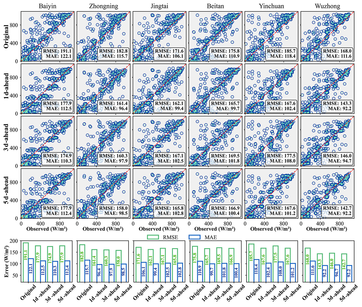
We validated the generalization of the QM-TPA-LSTM model by correcting GHI forecasts at six geographically diverse NSRDB sites. The correction results shown in Fig. 10 indicate that the model consistently reduced the error in the raw WRF forecasts across all external test sites and forecast horizons. Specifically, the model achieved maximum reductions in RMSE and MAE of 15.1 % and 17.4 %, respectively, at different sites. These results provide compelling evidence that the model can effectively enhance GHI correction accuracy, even when applied to other geographical locations and data sources (e.g., NSRDB). In conclusion, our local and multi-site validations demonstrate that the proposed hybrid framework is a generalizable and effective tool for post-processing GHI in numerical weather forecasts.

Figure 10 Evaluation of correction results using NSRDB data at multiple sites.

It should be acknowledged that the current QM-TPA-LSTM model operates as a purely statistical post-processing approach without explicitly incorporating physical variables such as aerosol optical depth, cloud fraction, or cloud optical thickness. While this statistical framework effectively reduces systematic NWP biases and captures temporal patterns in GHI errors, it lacks direct physical interpretability regarding the underlying atmospheric processes. The model learns implicit relationships between NWP outputs and observed GHI, but cannot explicitly attribute correction magnitudes to specific physical factors such as aerosol scattering or cloud attenuation. Future work could enhance physical interpretability by integrating satellite-derived aerosol and cloud products as additional input features, or by developing physics-guided correction schemes that explicitly model the radiative transfer processes affected by atmospheric constituents.

4 PV Power Forecasting and Evaluation

A comparative study was designed to validate the PINNs-iTransformer using operational data from a station in Zhongwei. The overall forecasting architecture is depicted in Fig. 11. The experimental protocol involved partitioning the dataset into training (80 %), validation (10 %), and testing (10 %) sets to prevent information leakage. We benchmarked our proposed PINNs-iTransformer against a suite of models representing distinct strategies for integrating physical principles with deep learning (iTransformer, Physics-iTransformer, PC-iTransformer). Performance was systematically evaluated across multiple forecast horizons: 6 h, 1, 3, and 5 d. Figures 12–14 demonstrate that the PINNs-iTransformer architecture consistently outperformed all competing models, confirming its superior predictive accuracy.

Figure 11 Schematic of the PV power forecasting framework.

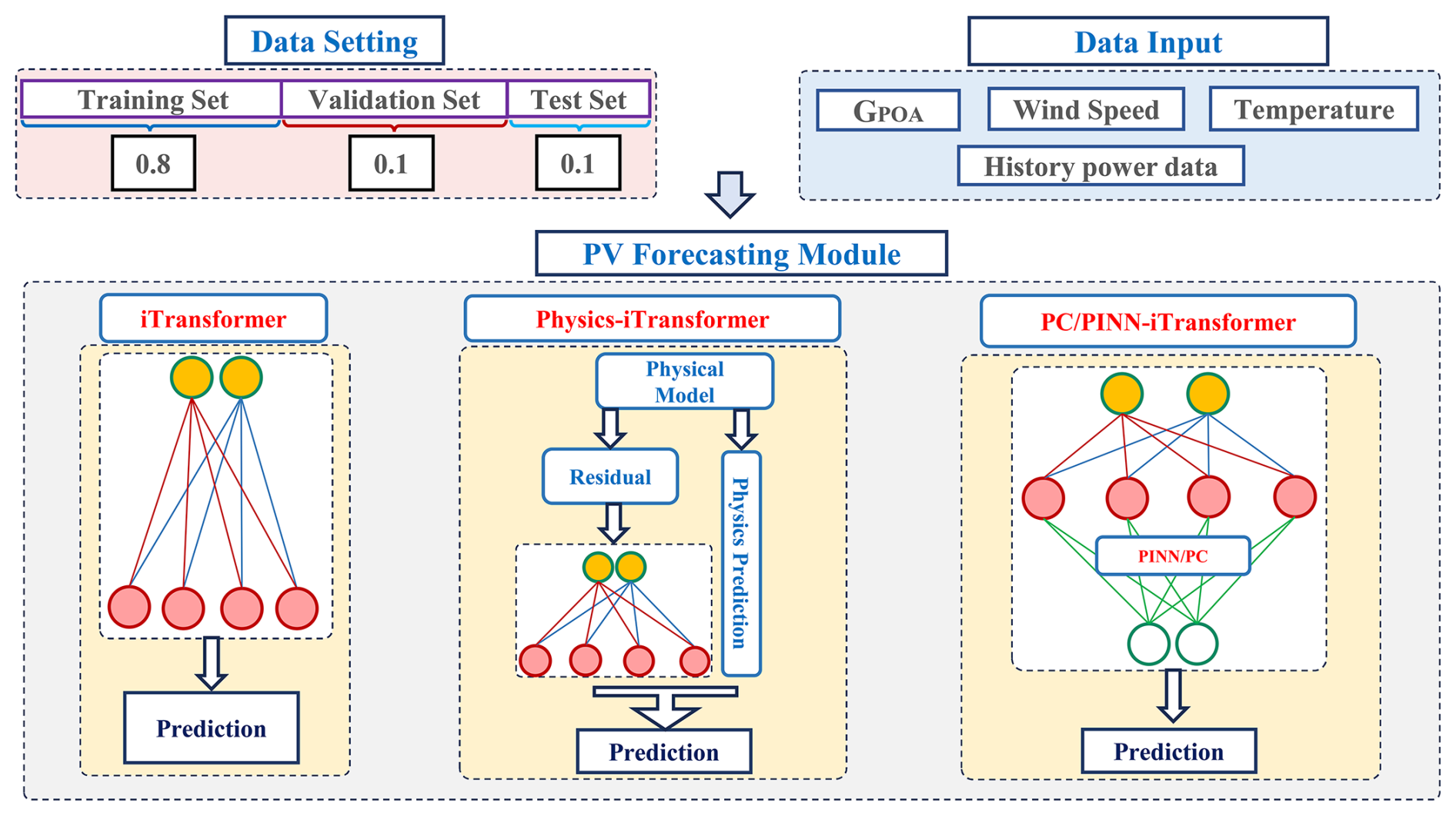
Figure 12 presents a comprehensive performance evaluation of the four primary forecasting models across multiple horizons. The analysis reveals a clear hierarchy of performance. The serial hybrid model (Physics-iTransformer) exhibited the poorest performance, with its error metrics (R, MAE, RMSE) significantly higher than those of other models. This suggests that a simple residual correction framework is prone to error accumulation and amplification. The purely data-driven iTransformer occasionally generated physically implausible negative power values, a common artifact of deep learning models lacking physical boundary constraints. In stark contrast, models incorporating physical knowledge demonstrated markedly superior reliability. Both the PC-iTransformer and our proposed PINNs-iTransformer outperformed the baseline models. Notably, the PINNs-iTransformer achieved the best overall performance, consistently yielding the highest R and the lowest MAE and RMSE across all forecast horizons. This result supports the hypothesis that integrating physical differential equations deeply into the network architecture, as the PINNs framework does, substantially enhances model generalization and predictive accuracy.

Figure 12 Time series plot of PV power predictions and error histogram evaluation.

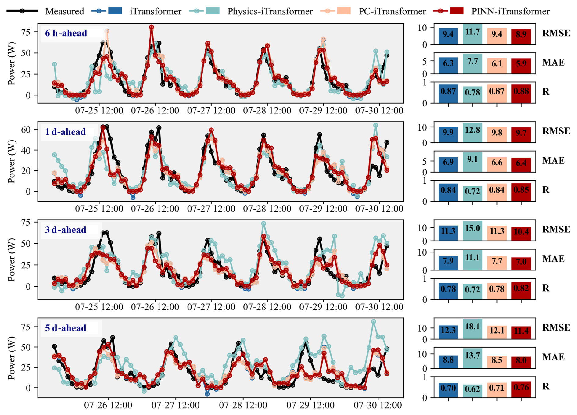
The predictive accuracy of all models degrades over longer forecast horizons, a deterioration attributable to three factors. First, cumulative error in the WRF-derived GHI propagates through the forecast, directly impairing power prediction. Second, the capacity of neural networks to maintain long-term temporal dependencies inherently diminishes across extended sequences. Finally, the limited training dataset constrains the model's ability to learn features robust enough for long-range inference, amplifying prediction errors.

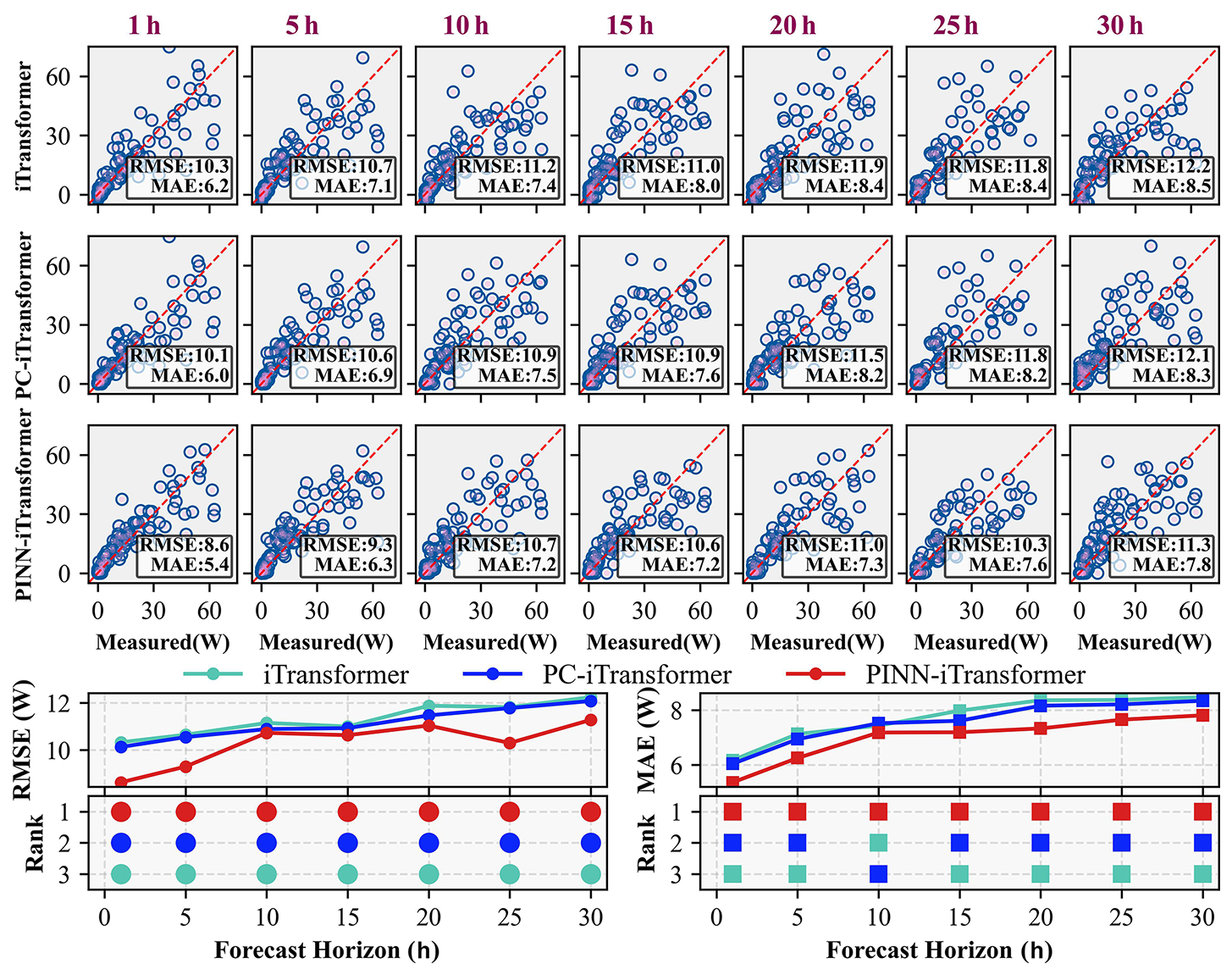
Furthermore, to better reflect real-world engineering applications and address the computational cost of WRF simulations, specifically, the resource redundancy from short rolling steps needed to avoid “spin-up” errors, we used a 5 d rolling WRF forecast to evaluate performance. As shown in Fig. 13, the PINNs-iTransformer model's predictions align more closely with the 1:1 line than the benchmarks. Across all forecast horizons, the model consistently outperforms all benchmark models, reducing RMSE and MAE by up to 15.5 % and 12.44 %, respectively. Notably, while prediction errors for all models increase with the forecast horizon, the PINNs-iTransformer maintains the lowest RMSE and MAE.

Figure 13 Multi-step PV power forecasting performance using a 5-day WRF forecast.

The proposed PINNs-iTransformer was evaluated against a diverse set of benchmarks, including LSTM (Yang et al., 2025), the frequency-domain-based TimesNet (Yu et al., 2025), a hybrid model integrating an attention mechanism, CNN-Attention-BiGRU (CA-BiGRU) (Dai et al., 2024), and the multilayer perceptron-based TSMixer (Ekambaram et al., 2023). All models were evaluated using the same multi-step forecasting tasks. The results, presented in Fig. 14, clearly demonstrate the outstanding performance of the PINNs-iTransformer. Its RMSE and MAE are significantly lower across all specified forecast horizons than those of all benchmark models.

Figure 14 Performance comparison of different models for multi-step forecasting.

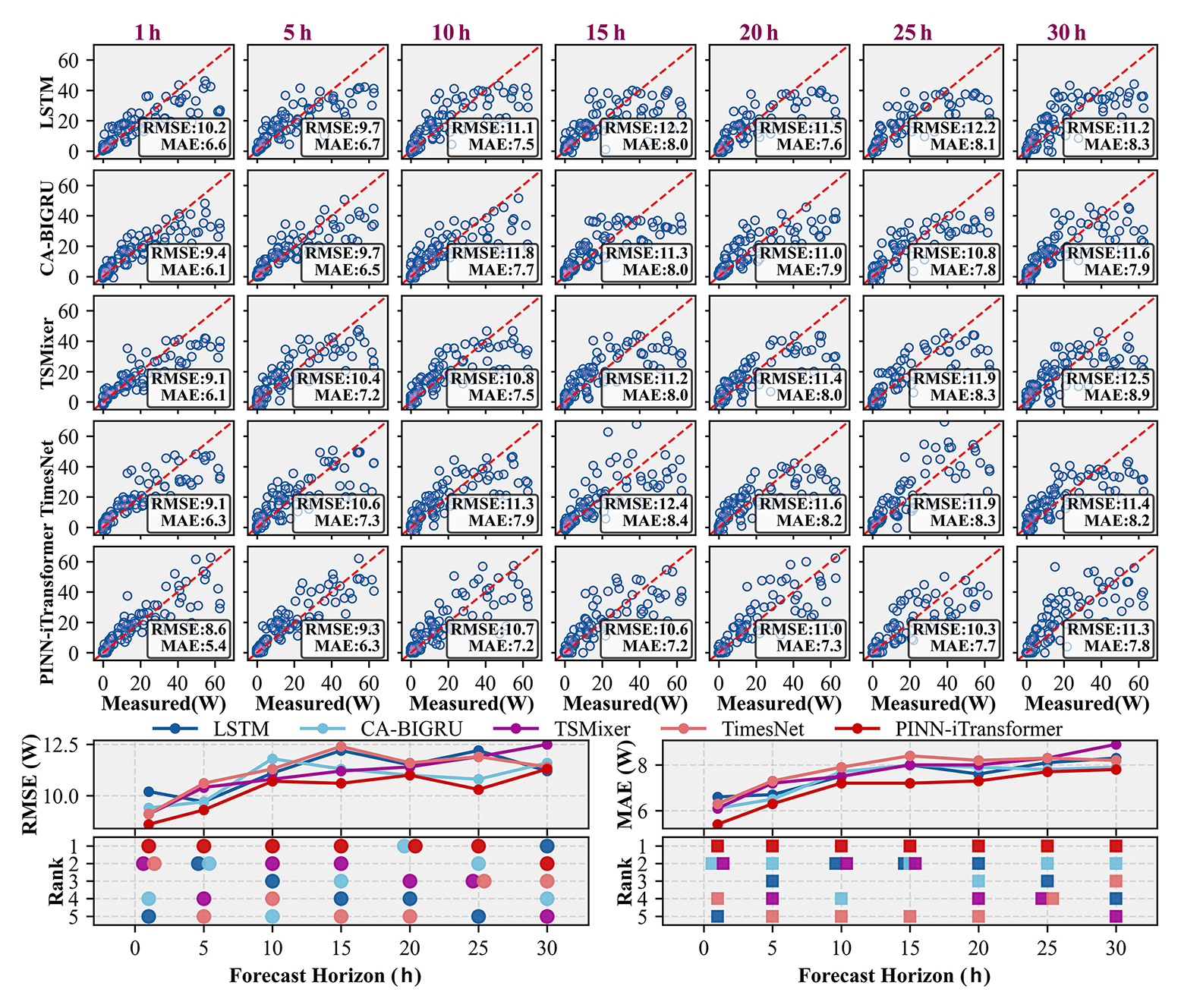
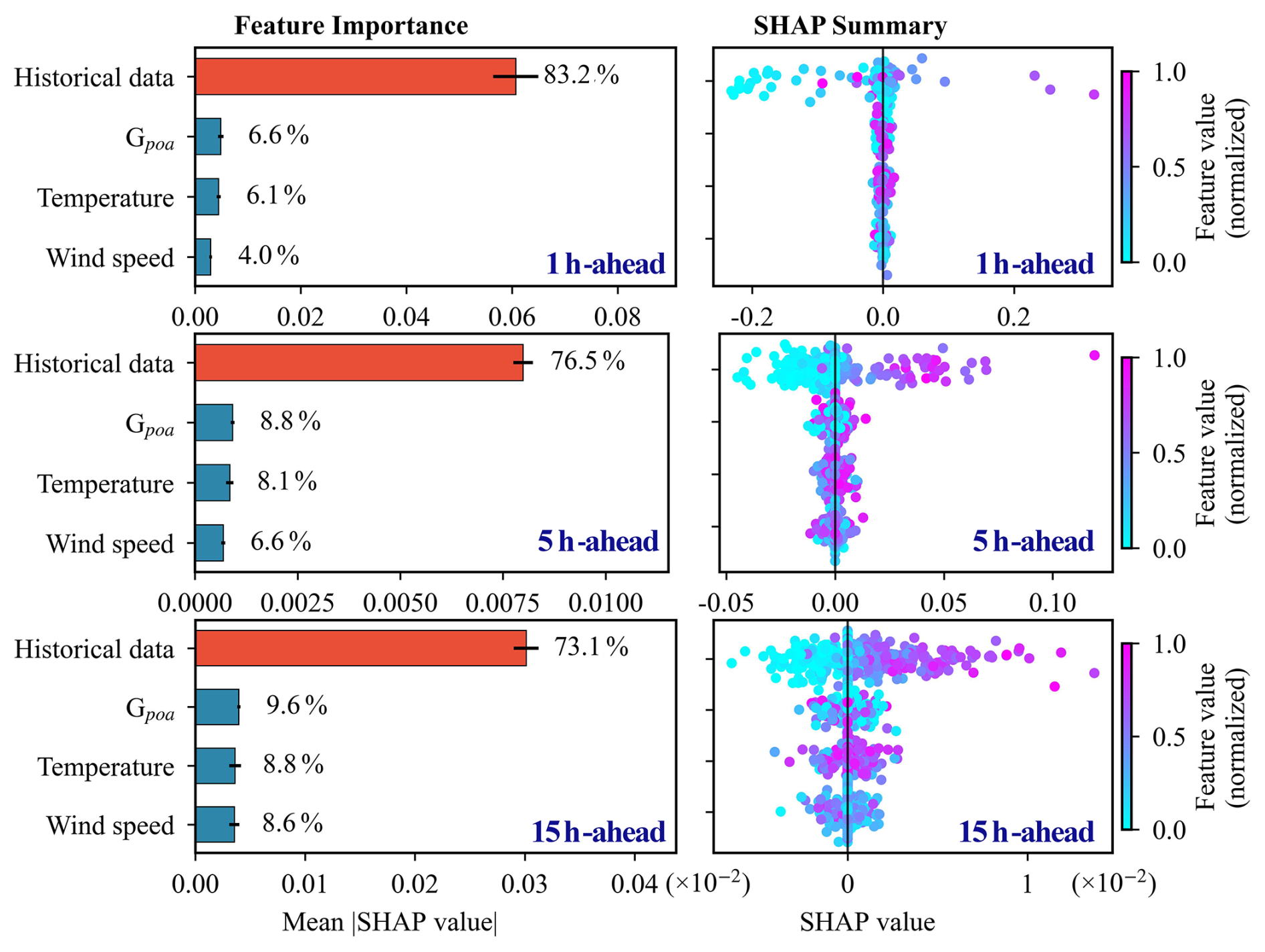
Figure 15 Left panels (top to bottom): distributions of feature importance at forecast horizons of 1, 5, and 15 h; right panels (top to bottom): SHAP beeswarm plots at forecast horizons of 1, 5, and 15 h.

Furthermore, the improved multi-scale PV power forecasting demonstrated in this study has significant implications for power system operations. As emphasized in previous reviews (Antonanzas et al., 2016; Iheanetu, 2022), forecasts at different time scales serve distinct operational purposes: day-ahead forecasts (24–120 h) support unit commitment decisions and electricity market participation; intra-day forecasts (6–24 h) facilitate energy storage scheduling and real-time balancing; and ultra-short-term forecasts (1–6 h) are critical for automatic generation control and frequency regulation. These operational benefits underscore the practical value of integrating physics-informed approaches into PV forecasting systems.

5 Analysis of key influencing factors and practical effort in forecasting

Beyond predictive metrics, we examine the model's physical consistency and robustness. This section analyzes the sensitivity of physical constraints, interprets feature dependencies, and assesses temporal transferability, followed by a discussion of operational uncertainties and limitations.

The physical loss weight serves λ as a critical hyperparameter that governs the trade-off between data-driven fidelity and adherence to theoretical constraints. To investigate the impact of the physics-informed constraint, we conducted a sensitivity analysis on the λ. Figure S2 shows the prediction error and learned coefficient k across varying λ values (10⁻⁴ to 10°). As shown in Fig. S2a–d, the model exhibits clear sensitivity to λ. For λ<0.01, both RMSE and MAE remain consistently below the baseline iTransformer (dashed lines). In this regime, the physical loss acts as a soft regularizer, embedding physical consistency without overriding data-driven features. When λ>0.05, prediction errors increase noticeably because the simplified ODE cannot fully capture real-world weather stochasticity. Excessive physical loss weighting forces the model to adhere too strictly to the simplified trend, resulting in underfitting. Figure S2e shows the evolution of the relaxation coefficient k, implemented as a learnable parameter representing the adaptive coupling strength between theoretical equilibrium (P_eq) and predicted power (P_pred). The coefficient converges to a stable range (approx. 0.9–0.96) rather than fluctuating randomly, indicating that the model successfully learns an intrinsic restoration rate reconciling the simplified physical theory with observed data patterns.

We conducted SHAP analysis across forecast horizons from 1 to 15 h to examine the physical consistency of learned representations (Fig. 15). The analysis reveals a physically coherent transition in feature reliance. At the 1 h horizon, historical power accounts for 83.2 % of the predictions, reflecting strong temporal autocorrelation. This contribution decreases to 73.1 % at 15 h, while meteorological variables show increased importance: G_POA (9.6 %), temperature (8.8 %), and wind speed (8.6 %). This pattern aligns with the expected decline in the effectiveness of persistence-based forecasting at extended horizons. Feature dependence analysis further reveals non-linear interactions consistent with PV physics, including temperature-induced efficiency losses and wind-driven convective cooling modulated by irradiance levels. Bootstrap resampling confirms high attribution stability (R² = 0.9992 across 1000 iterations), indicating that the model captures robust physical relationships.

Due to experimental constraints, direct photovoltaic power forecasting for 2025 was not feasible. To assess model transferability, we obtained solar irradiance data for July-August 2025 from six stations via the NASA POWER database (The data was obtained from the POWER Project's Hourly 2.5.25 version on 1 July–31 August 2025), performed WRF simulations, and applied the QM-TPA-LSTM correction framework. Results (Figs. S3–S9) demonstrate that QM-TPA-LSTM consistently outperforms raw WRF predictions and all benchmark models across all stations, with substantial reductions in RMSE and MAE. Despite being trained on 2020 data, the correction methodology remains effective for 2025 forecasts at geographically diverse locations, indicating robust temporal and spatial generalizability.

Several limitations define the current operational scope of the proposed framework. First, the PV power forecasting validation is conducted at a single station in a semi-arid, high-irradiance environment. While this setting provides a representative benchmark for clear-sky-dominated regions, the model's performance under high cloud-variability conditions remains to be evaluated. Second, the physics-informed architecture theoretically constrains the model to learn generalizable relationships by embedding universal PV principles (Karniadakis et al., 2021). The SHAP analysis provides supporting evidence of physical consistency; however, these theoretical and interpretability-based arguments do not substitute for empirical multi-site validation. Third, the model is optimized for short- to medium-term operational forecasting (up to 5 d) and does not account for long-term factors, such as panel degradation or climate drift, that are relevant to decadal projections. Additionally, cross-validation with independent satellite products (e.g., SolarGIS) was not performed due to data availability constraints during the measurement campaign. Future work should prioritize: (i) multi-site validation across diverse climatic zones and PV system configurations, (ii) assessment of transfer learning capabilities, and (iii) integration of additional satellite-based irradiance products for independent verification.

To apply the proposed framework to a new site in a production environment, the practical implementation is primarily divided into meteorological setup and operational inference. For the initial setup, running WRF requires a high-performance computing environment (e.g., 128-core CPU cluster), taking approximately 3 h for a 72 h forecast. Subsequent data processing, model training, and evaluation can be efficiently executed on standard consumer-grade hardware (e.g., an Intel Core i5-13600KF CPU, 16 GB RAM, and an NVIDIA RTX 2060 GPU). On such hardware, the GHI correction phase takes roughly 2 min, and the PINNs-iTransformer training takes approximately 3–5 min. Daily operational inference is computationally negligible (< 1 s). Applying this framework to a new region extends beyond routine codebase modifications, requiring a rigorous, three-step re-determination process: (1) updating WRF domain coordinates and terrain files; (2) adapting the data ingestion pipeline to accommodate local PV specifications and weather observations; and (3) thoroughly retraining the QM-TPA-LSTM and PINNs-iTransformer architectures with local datasets. This mandatory retraining is crucial to ensuring that the framework's physical consistency remains intact in any new environment.

6 Conclusion

This study proposes a physics-informed real-time forecasting framework designed to overcome key limitations – such as poor generalizability and physical inconsistency – in conventional data-driven approaches for photovoltaic (PV) power forecasting. The framework establishes an end-to-end prediction pipeline that integrates high-resolution numerical weather prediction (NWP), a novel global horizontal irradiance (GHI) bias correction model, and a physics-constrained deep learning architecture.

First, the hybrid QM-TPA-LSTM model synergistically combines statistical quantile mapping with deep temporal pattern extraction, achieving superior GHI bias correction accuracy across forecasting horizons ranging from 6 h to 5 d, outperforming existing methods, including standalone neural networks and Kalman filter (KF) models. Furthermore, the framework exhibits strong transferability, maintaining consistent performance across multiple stations and temporal validation periods.

Second, the newly developed PINNs-iTransformer architecture for power forecasting explicitly incorporates physical principles into the network design. This integration ensures physically plausible predictions, effectively guiding the learning process and substantially improving model generalization and stability. As a result, the PINNs-iTransformer consistently outperformed state-of-the-art time-series models across all evaluated forecast horizons.

While the current framework demonstrates promising performance in PV forecasting, accurate prediction remains challenging. Future work should focus on: (i) acquiring additional PV station data for multi-site validation, (ii) assessing model applicability under diverse climatic conditions, and (iii) conducting long-term forecast verification.