Development and preliminary validation of an EnKF-like image assimilation system for the Common Land Model

Accurate representation of both the location and magnitude of soil moisture anomalies in land surface model initial conditions is crucial for simulating land–atmosphere interactions. However, traditional point-based land data assimilation methods primarily adjust anomaly magnitude, with limited capability to improve spatial structure due to the single-column design of most land surface models. This study develops an assimilation approach that optimizes the spatial patterns of soil moisture. For the Common Land Model (CoLM), soil moisture fields are treated as images, and a curvelet transform is introduced as the image observation operator. Ensemble methods are used to dynamically estimate errors in the image structure, and the background field is updated in image space using a Kalman filter framework, forming an EnKF-like land surface image assimilation system. Assimilation experiments show that this system effectively exploits the multi-scale spatial information contained in observations, improving soil moisture spatial patterns while reducing magnitude errors. After assimilation, the spatial correlation of surface soil moisture with GLDAS increases from 0.4 to 0.8, and the unbiased RMSE decreases from 0.12 to 0.06 m³ m⁻³. Through vertical propagation, correlations rise from 0.35 to 0.55 at 10–40 cm and from 0.25 to  0.4 at 40–100 cm. Independent validation using in-situ stations shows correlation increases from 0.153 to 0.425 in China and from 0.142 to 0.504 in the United States. These results highlight the potential of the proposed system to improve land surface initial fields and strengthen weather and climate predictions.

1 Introduction

Soil moisture is a key variable in the Earth's climate system and modulates surface energy and water fluxes to influence land-atmosphere interactions (Seneviratne et al., 2010). At the weather scale, spatial gradients of soil moisture can initiate mesoscale circulations, thereby modulating convective development and organizing precipitation patterns (Taylor, 2015; Wanders et al., 2019). On subseasonal-to-seasonal (S2S) timescales, soil moisture exhibits long-term memory that is a vital source of predictability for S2S outlooks (Esit et al., 2021). This persistence preconditions the land–atmosphere system such that, via positive soil-moisture–temperature feedbacks, the intensity and duration of heat waves and droughts can be amplified (Miralles et al., 2014; Schumacher et al., 2022). Therefore, accurate soil moisture is important for improving weather forecasts, enhancing climate prediction skill, and issuing timely early warnings of extreme events (Rahmati et al., 2024).

Soil moisture data assimilation integrates observational datasets with land surface model (LSM) simulations to provide more accurate and model-consistent initial conditions, thereby improving the performance of LSM (Kolassa et al., 2017; Shan et al., 2024; Zhou et al., 2022). A large body of research has shown that land data assimilation, when combining satellite remote sensing and in-situ soil moisture observations, can improve the quality of LSM initial conditions and thereby enhance estimates of surface energy balance, evapotranspiration, and precipitation forecasts (Draper and Reichle, 2019; Lin et al., 2017; Zhao et al., 2025).

Soil moisture often influences the atmosphere through regionally coherent anomalies that act as a large-scale forcing on atmospheric processes (Barton et al., 2025; Cheng et al., 2021; Klein and Taylor, 2020). However, because LSMs operate as single-column systems, most land data assimilation studies are performed point by point (McLaughlin et al., 2006). Under such a point-based assimilation framework, soil moisture values and their error characteristics exhibit strong spatial heterogeneity due to the combined effects of soil texture, vegetation type, and terrain elevation (Li et al., 2022; Li et al., 2024). As a result, point-wise land data assimilation can disrupt the dominant spatial organization of soil moisture anomalies in the analysis fields, limiting the ability of land data assimilation to improve land–atmosphere interaction processes (Dan et al., 2020; Klein et al., 2015; Tong, 2018).

To improve the spatial structure of the analysis fields, Le Dimet et al. (2015) proposed the image assimilation method. Building on this concept, Shen et al. (2024) introduced image assimilation into land data assimilation by using the curvelet transform to extract large-scale spatial features from observational images as a weak constraint, and developed a new land surface image assimilation system within a variational framework. Through practical assimilation experiments using the CoLM (Common Land Model), their results demonstrated that the image-based approach can effectively enhance the spatial accuracy of the analysis fields. However, this method assumes that the large-scale spatial structures in the observations are error-free and does not account for the influence of observation errors on these structures. In practice, both satellite remote sensing data and reanalysis products inevitably contain systematic biases and random errors, and directly treating structural information at specific scales as truth may introduce observation errors into the analysis fields (Dorigo et al., 2015; Ling et al., 2021; Qin et al., 2022).

By contrast to Shen et al. (2024), which emphasized large-scale soil-moisture structure, the move toward higher-resolution prediction has elevated the need for accurate land-surface initial conditions from weather to S2S and longer-range forecasts (Duan et al., 2025; Nair et al., 2024; Xue et al., 2021). When serving the purposes of short-term weather forecasting or longer-term climate prediction, land surface assimilation may need to address structure information at different scales. Moreover, land surface assimilation aims not only to incorporate relatively accurate observational information but, more importantly, to establish analysis fields suitable for LSMs. This implies that for LSMs operating at different spatial resolutions, it is necessary to selectively enhance the accuracy of different scales based on the model's capability to simulate characteristics at various scales, thereby establishing an image assimilation system appropriate for the model. Therefore, the primary objective of this study is to develop a more universal image assimilation system by objectively incorporating multiscale information from observations.

To address the limitations noted above, this study seeks to develop a more complete image-based assimilation approach. The key innovation lies in introducing a full error estimation framework that converts both background and observation errors from the observation space to the image space. The linearity and invertibility of the curvelet transform allow the error covariance matrix in the observation space to be accurately mapped into the image space, establishing a link between errors in the observation domain and those in the spectral domain. This enables a quantitative representation of errors across different structural scales and allows the image assimilation system to more objectively adjust the confidence assigned to each scale of structural information. By further using the orthogonality of multi-scale components in curvelet analysis, an image-based land data assimilation system suitable for global LSMs is constructed following the Kalman filter framework. Using the CoLM and the newly developed assimilation system, and with GLDAS soil moisture reanalysis as reference data, this study provides an initial assessment of how the new image assimilation approach improves CoLM's soil moisture simulations, providing a useful reference for applying image assimilation methods in global LSMs.

The remainder of this paper is organized as follows. Section 2 introduces the soil moisture and precipitation datasets used in this study. Section 3 describes the construction of the EnKF-like image assimilation system and the design of the assimilation experiments. Section 4 presents the results of idealized experiments to evaluate the effectiveness of the system in improving model forecast skill. Section 5 provides a summary and discussion.

2 Data

2.1 GLDAS reanalysis data

The GLDAS, developed by the NASA Goddard Earth Sciences Data and Information Services Center (GES DISC), integrates multi-source observational data with LSMs to generate global land surface variable products (Rodell et al., 2004). GLDAS consists of three major versions: GLDAS-2.0, GLDAS-2.1, and GLDAS-2.2. It provides s simulations from several LSMs, including Noah, CLM, VIC, Mosaic, and Catchment.

Among them, GLDAS-2.1 is driven by a combination of meteorological forcing datasets, including atmospheric analysis fields from the NOAA Global Data Assimilation System (GDAS), daily precipitation data from the Global Precipitation Climatology Project (GPCP), and radiation data from the Air Force Weather Agency's (AFWA) Agricultural Meteorology modeling system (AGRMET). This version spans from 2000 to the present and is available at spatial resolutions of 1° × 1°, and 0.25° × 0.25°, with a temporal resolution of 3 h. The Noah model in GLDAS-2.1 provides four-layer soil moisture simulations corresponding to depth ranges of 0–10, 10–40, 40–100, and 100–200 cm.

In this study, we use the top three soil moisture layers from the Noah model in GLDAS-2.1, covering the period from June to August 2022. Since the spatial resolution of the CoLM used in this study is 1.4°, the GLDAS data are resampled to the model resolution using bilinear interpolation to ensure spatial consistency between datasets.

It should be noted that resampling the 0.25° GLDAS data onto the lower-resolution 1.4° model grid using bilinear interpolation may introduce a smoothing effect. In regions with highly heterogeneous land surface conditions, this interpolation may weaken local soil moisture extremes and blur small-scale spatial gradients. However, this compromise is mainly constrained by the spatial resolution of the current land surface model. To ensure consistency in spatial scale between the observation field and the model background field, resampling is a necessary preprocessing step. In future applications with higher-resolution land surface models, the impact of this smoothing effect is expected to be substantially reduced.

2.2 In-situ soil moisture observations

This study uses high-quality in situ soil moisture observations from two sources. The first is the automatic soil moisture observation network maintained by the China Meteorological Administration (CMA), and the second is the International Soil Moisture Network (ISMN).

The CMA's observation network was initiated in 2009 and has been gradually put into operational use since 2011, forming a nationwide system for routine soil moisture monitoring. The network employs Frequency Domain Reflectometry (FDR) technology and deploys high-precision sensors at standardized depth intervals (0–10, 10–20, 20–30, 30–40, 40–50, 50–60, 70–80, and 90–100 cm) to measure volumetric soil water content at high temporal resolution (Wang et al., 2018). Observations are recorded hourly and reported as 10 min averages preceding each hour. This dataset offers advantages in both temporal resolution and spatial coverage. In this study, we use 10 cm depth soil moisture observations from 2878 stations for the period June to August 2022.

ISMN initiated by the Vienna University of Technology, is the world's largest open-access in situ soil moisture database. It supports the validation of LSMs and the calibration of satellite soil moisture products (Dorigo et al., 2021). ISMN integrates soil moisture data from 71 independently operated networks across 58 countries, comprising over 2800 stations, with records dating back to 1952. All data are standardized and provided in hourly volumetric soil water content. In this study, we select 10 cm soil moisture observations from the ISMN network located in the United States for the period from June to August 2022, including 148 stations used for validation.

2.3 Precipitation data

This study uses a high-precision station–satellite merged precipitation analysis product developed by Shen et al. (Shen et al., 2014) as the precipitation observational dataset. The product is generated using the Probability Density Function–Optimal Interpolation (PDF-OI) algorithm, which merges hourly precipitation observations from over 30 000 automatic weather stations operated by the CMA with satellite-based precipitation estimates from the Climate Prediction Center Morphing technique (CMORPH) developed by NOAA's Climate Prediction Center. The resulting gridded dataset has a temporal resolution of one hour and provides high-quality precipitation fields suitable for LSM applications.

3 Methodology and experimental design

3.1 CoLM

CoLM was developed by Dai et al. (2003) based on the LSM from the National Center for Atmospheric Research (NCAR LSM) (Bonan et al., 2002), the Biosphere–Atmosphere Transfer Scheme (BATS) (Dickinson et al., 1993), and the IAP94 model from the Institute of Atmospheric Physics, Chinese Academy of Sciences (Dai and Zeng, 2007). The model is designed to simulate the exchange of energy, carbon, and water between the land surface and the atmosphere. It comprehensively incorporates biophysical, biogeochemical, ecological, and hydrological processes, enabling realistic simulation of soil temperature, soil moisture, surface heat fluxes, and other land surface variables.

At present, two major versions of CoLM have been released, CoLM2005 and CoLM2014. Compared to CoLM2005, CoLM2014 introduces several important updates across multiple modules. In runoff parameterization, CoLM2014 replaces the original BATS-based scheme with the SIMTOP runoff model derived from TOPMODEL (Niu et al., 2005). It also implements a new-generation multi-layer lake model, replacing the simpler two-layer scheme used in CoLM2005 (Dai et al., 2018).

In this study, the offline mode of CoLM2014 is employed. The model is run at a horizontal resolution of 1.4° × 1.4°, with 10 soil layers and up to 5 snow layers in the vertical dimension. Atmospheric forcing variables required by the model include downward shortwave and longwave radiation, surface air temperature, specific humidity, near-surface wind speed, surface pressure, and precipitation rate. These inputs are obtained from the near-surface reanalysis dataset provided by the European Centre for Medium-Range Weather Forecasts (ECMWF), covering the period from 1979 to 2022. Before conducting the experiments, the model is driven cyclically for 360 years using the forcing data to bring the system to equilibrium.

3.2 Multi-scale curvelet analysis method

The curvelet transform, proposed by Candès and Donoho (2000), is a signal and image processing technique designed for multi-scale geometric analysis. It was developed to overcome the limitations of wavelet transforms in representing geometric features such as edges and curves in two-dimensional or higher-dimensional signals. By decomposing two-dimensional data into basis functions at multiple scales and orientations, the curvelet transform efficiently identifies and extracts curvilinear structures and localized variations. At scale j, the curvelet basis function φ_j is constructed using a radial window function W and an angular window function V, and is defined as follows:

$$\begin{array}{}\text{(1)}& {\mathit{\phi }}_j\left(\mathit{\omega }\right)={\mathrm{2}}^{-\frac{\mathrm{3}j}{\mathrm{4}}}W\left({\mathrm{2}}^{-j}\mathrm{|}\mathit{\omega }\mathrm{|}\right)V\left({\displaystyle \frac{{\mathrm{2}}^{⌊\frac{j}{\mathrm{2}}⌋}{\mathit{\theta }}_{\mathit{\omega }}}{\mathrm{2}\mathit{\pi }}}\right)\end{array}$$

The normalization factor ${\mathrm{2}}^{-\mathrm{3}j/\mathrm{4}}$ ensures that the basis functions are properly scaled in the L² space. The radial window function W facilitates multi-scale decomposition of the signal, while the angular window function V determines directional selectivity and resolution. The scale parameter j defines the effective support of the curvelet basis functions in the frequency domain, with an approximate frequency width of 2^j and frequency length of ${\mathrm{2}}^{j/\mathrm{2}}$. Directional basis functions are then generated through rotation operations, and spatial localization is achieved via translation, ultimately forming the complete curvelet frame:

$$\begin{array}{}\text{(2)}& {\mathit{\phi }}_{j,k,l}\left(x\right)={\mathit{\phi }}_j\left({\mathbf{R}}_{{\mathit{\theta }}_{j,l}}\left(x-b_k^{(j,l)}\right)\right)\end{array}$$

where φ_j is the mother curvelet, j denotes the scale, k represents the translation parameter, l denotes the orientation, and x is the coordinate of a sample grid point in two-dimensional space. ${\mathbf{R}}_{{\mathit{\theta }}_{j,l}}$ is the rotation matrix with angle θ_j,l, and $b_k^{(j,l)}$ is the translation parameter. For a discrete two-dimensional signal f(x), the curvelet transform represents it as a linear combination of curvelet functions at different scales, orientations, and positions. The curvelet coefficients are calculated as follows:

$$\begin{array}{}\text{(3)}& c_{j,k,l}={\sum }_{x\in \mathrm{\Omega }}f\left(x\right){\mathit{\phi }}_{j,k,l}\left(x\right)\end{array}$$

where Ω denotes the set of grid points in two-dimensional space, ${\mathit{\phi }}_{j,k,l}\left(x\right)$ is the curvelet function, and $c_{j,k,l}$ is the curvelet coefficient corresponding to scale j, position k, and orientation l. The coefficients obtained from the curvelet transform can be reconstructed back to the original space through the inverse transform, which is expressed as follows:

$$\begin{array}{}\text{(4)}& f\left(x\right)={\sum }_{j=\mathrm{1}}^J{\sum }_{l=\mathrm{1}}^{L_j}{\sum }_{k=\mathrm{1}}^{K_{j,l}}{c}_{j,k,l}{\mathit{\phi }}_{j,k,l}\left(x\right)\end{array}$$

where J is the total number of scales, L_j denotes the number of orientations at scale j, and K_j,l denotes the number of positions at scale j and orientation l. Equation (4) shows that the original field can be reconstructed by summing the curvelet coefficients over all scales, orientations, and positions.

Similar to the PCA method commonly used in meteorological studies, curvelet analysis can also decompose the variable into several components with different spatial characteristics. PCA usually extracts leading modes according to the magnitude of variance contribution in time series, and these modes reflect the dominant spatial structures of the variable. In contrast, curvelet analysis uses predefined basis functions at different scales and orientations and projects the variable field at a given time onto these basis functions, thereby obtaining components with different scales and orientations. A single mode in curvelet decomposition can be interpreted as a spatial fluctuation feature within a certain orientation and scale range, and can therefore represent soil moisture variations at a specific spatial scale. In general, lower-order modes correspond to low-frequency signals and mainly reflect large-scale spatial distribution features, whereas higher-order modes correspond to higher-frequency components and describe smaller-scale spatial details. As subsequent modes are gradually introduced, curvelet analysis can resolve increasingly finer spatial structures.

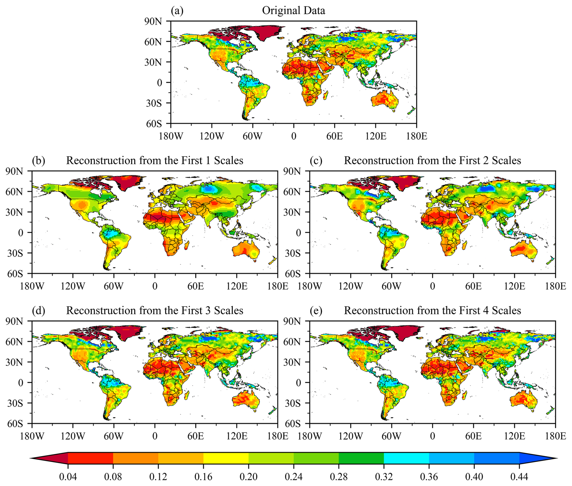
Figure 1 Spatial distribution of soil moisture from (a) the original image and reconstructed fields based on different curvelet coefficient modes: (b) the first mode, (c) the first two modes, (d) the first three modes, and (e) the first four modes on 2 June 2022.

The curvelet-derived spatial features are grouped according to the meteorological scale convention, from planetary-scale to large-scale and mesoscale features. These categories correspond, respectively to broad background patterns, regional structures, and finer variations associated with local heterogeneity. Figure 1 presents the spatial structure of global soil moisture fields reconstructed using curvelet transform modes at different scales. Figure 1a shows the original soil moisture distribution simulated by CoLM, exhibiting a clear latitudinal gradient in which soil moisture decreases from low to high latitudes over the Americas and Eurasia. When the reconstruction is performed using only the first curvelet mode (Fig. 1b), the image retains only the planetary-scale spatial features, capturing broad global patterns such as humid zones in the high latitudes of the Northern Hemisphere and arid regions in the tropics. However, much of the regional detail is lost. For example, over the Sahara Desert, the reconstruction yields only a single intensely arid center, with the influence of dryness gradually diminishing outward toward the desert margins. When the number of reconstruction modes increases to two (Fig. 1c), additional spatial features across multiple scales begin to emerge, and the internal structures of some large-scale systems become more distinctly defined. Taking the Sahara Desert again as an example, the previously unified arid center evolves into three distinct northeast–southwest-oriented moisture gradient zones, allowing for a more accurate delineation of the core arid region and its transitional boundaries. When three modes are included (Fig. 1d), the reconstructed image captures most of the key spatial structures from the original field, including the complex patterns over Central Asia, land–ocean contrasts in Australia, and the detailed structure of extreme aridity within the Sahara. Using the first four curvelet modes (Fig. 1e), the reconstructed field closely resembles the original image, not only accurately recovering large-scale patterns but also preserving mesoscale regional features. For example, the pronounced spatial heterogeneity over South America and the monsoon-influenced soil moisture gradients over East Asia are well represented. These results demonstrate that the curvelet transform effectively decomposes complex spatial fields into scale-separated structural components, providing a basis for incorporating observational spatial structure into data assimilation frameworks.

3.3 EnKF-like image assimilation

In contrast to traditional assimilation approaches that concentrate on modifying variable magnitudes, image assimilation techniques focus on recalibrating spatial characteristics across multiple scales. The core difficulty resides in disentangling variables into clearly defined spatial structural attributes. Because variable magnitudes fluctuate with meteorological systems and temporal progression, achieving objective separation of structural features relying exclusively on magnitude values presents considerable challenges. Yet when variables are transformed from observation space to spectral space, areas of structural variation map directly onto domains with elevated spectral coefficients. Accordingly, this investigation implements curvelet analysis utilizing anisotropic basis functions to transition variable fields into spectral space, wherein spectral coefficients at distinct frequencies correspond to structural constituents at separate scales. Land surface assimilation thereby becomes directly redefinable as spectral coefficient assimilation. A significant advantage of the curvelet transformation stems from its capacity for precise inverse representation through analytical expressions, securing complete reversibility during data conversion between observational and spectral domains. Following assimilation procedures in spectral space, the synthesized results can therefore be reconstructed into the original observation space while maintaining informational completeness. The orthogonal nature of the curvelet transform across scales further permits autonomous handling of individual spatial modes, successfully eliminating cross-scale interference among fluctuating components.

To distinguish the proposed framework from the conventional EnKF, which updates the full ensemble state in physical model space, we refer to it as an “EnKF-like” assimilation framework. Unlike the EnKF, this method does not estimate state-variable error covariances directly in physical space. Instead, the forecast ensemble is mapped into curvelet spectral space, where the error covariance of the spectral coefficients is dynamically estimated from the ensemble samples. Taking advantage of the approximately independent properties of the curvelet basis functions, the analysis update is then performed in spectral space using the standard Kalman filter equation. For computational simplicity, the framework does not include a full ensemble update after the analysis step; therefore, it is termed “EnKF-like”.

This study employs the EnKF method to improve assimilation of different spectral coefficients in spectral space. The EnKF estimation formula for the analysis field X^a is:

$$\begin{array}{}\text{(5)}& {\mathbf{X}}^{\mathrm{a}}={\mathbf{X}}^{\mathrm{f}}+\mathbf{K}(\mathbf{y}-\mathbf{H}({\mathbf{X}}^{\mathrm{f}}\left)\right)\end{array}$$

where X^f represents the model background field, and H is the observation operator matrix that maps the model state to observation space. The Kalman gain matrix K is obtained through:

$$\begin{array}{}\text{(6)}& \mathbf{K}={\mathbf{BH}}^{\mathrm{T}}({\mathbf{HBH}}^{\mathrm{T}}+\mathbf{R}{)}^{-\mathrm{1}}\end{array}$$

where B represents the background error covariance matrix of model states, and R is the observation error covariance matrix.

In practical assimilation applications, error estimation of spectral coefficients for both observations and background fields are the most critical component. Assimilation in spectral space requires estimating errors of spectral coefficients corresponding to different spatial modes. Using the ensemble-based error estimation approach of EnKF and the accurate decomposition capability of the curvelet transform, we can directly transform variable errors from observation space to spectral coefficient errors.

Leveraging the mathematical exactness of curvelet analysis, we can transform not only the structure of variables in physical space into spectral coefficients, but also the corresponding errors into coefficients in spectral space. In this EnKF-like assimilation framework, following the error estimation strategy of the EnKF, we first estimate the background error of soil moisture at each grid point in physical space, random perturbations with zero mean and a standard deviation corresponding to the physical-space error are added to the background soil moisture field, thereby generating an ensemble of perturbed members. Let the ith ensemble member in physical space be denoted as x_i ($i=\mathrm{1},\mathrm{2},\mathrm{\dots },N$), where N is the ensemble size. In this study, the ensemble size is set to N=50. By applying the curvelet transform operator C, these members are mapped one by one into spectral space, yielding the corresponding curvelet coefficients with errors:

$$\begin{array}{}\text{(7)}& c_i=C\left(x_i\right)\end{array}$$

The background error covariance matrix B in spectral space is dynamically estimated directly from the ensemble samples in spectral space:

$$\begin{array}{}\text{(8)}& \mathbf{B}={\displaystyle \frac{\mathrm{1}}{N-\mathrm{1}}}{\sum }_{i=\mathrm{1}}^N\left({\mathbf{c}}_i-\stackrel{\mathrm{‾}}{c}\right){\left({\mathbf{c}}_i-\stackrel{\mathrm{‾}}{c}\right)}^{\mathrm{T}}\end{array}$$

where $\stackrel{\mathrm{‾}}{c}$ denotes the ensemble mean of the curvelet coefficients, and the superscript T indicates matrix transpose. The observation error covariance matrix R is transformed in a similar manner. The standard deviations of the random perturbations are prescribed as 0.15 m³ m⁻³ for the background soil moisture field and 0.1 m³ m⁻³ for the observation field. In fact, owing to the orthogonality of different basis functions, the background error covariance B and observation error covariance R are diagonal in the spectral space. Thus, the unrealistic divergence of error impacts can be avoided, making the error localization and inflation procedure unnecessary.

After B and R are constructed, the assimilation system performs the EnKF analysis step in spectral space to compute the updated curvelet coefficients c^a. Finally, the inverse curvelet transform operator C⁻¹ is applied to map the updated curvelet coefficients back to physical space, thereby obtaining the final analyzed field:

$$\begin{array}{}\text{(9)}& x^{\mathrm{a}}=C^{-\mathrm{1}}\left(c^{\mathrm{a}}\right)\end{array}$$

Figure 2 Schematic Flowchart of the EnKF-like Image Assimilation System.

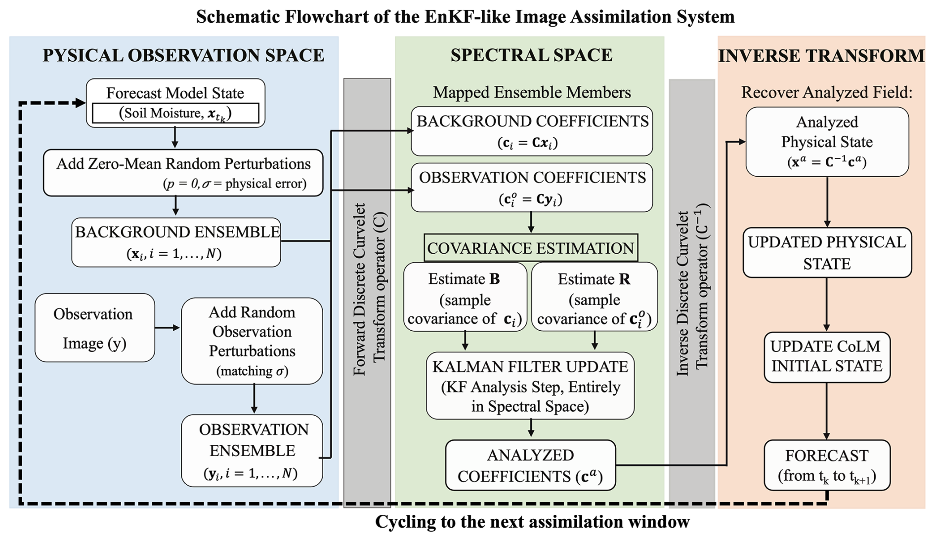
To provide a clearer illustration of the overall architecture of the curvelet-transform-based EnKF-like image assimilation system, we present a schematic flowchart in Fig. 2. As shown in Fig. 2, one assimilation cycle of the framework consists mainly of four key steps. First, in the physical space, the initial ensemble is generated by adding random perturbations to both the background field and the observation field. Second, the forward curvelet transform operator is applied to map the ensemble members from physical space to spectral space. Third, in spectral space, the background and observation error covariances are dynamically estimated from the ensemble samples, and the Kalman filter update is performed to obtain the analysis field of curvelet coefficients. Finally, the inverse curvelet transform is applied to convert the updated curvelet coefficients back to the physical space, thereby optimizing the spatial structure of the model state variables as a whole.

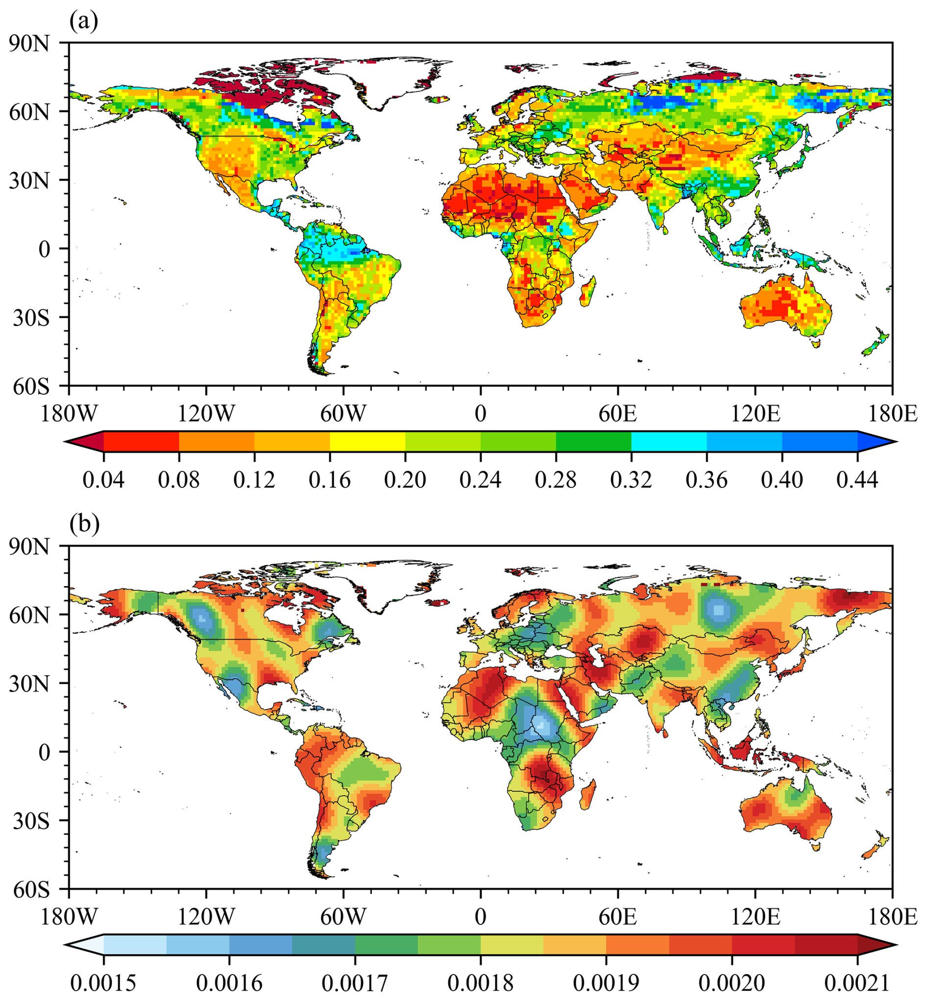
Figure 3 (a) Soil moisture background field and (b) difference between the background field and the reconstructed field after adding background error perturbations and applying first-mode curvelet inverse transformation.

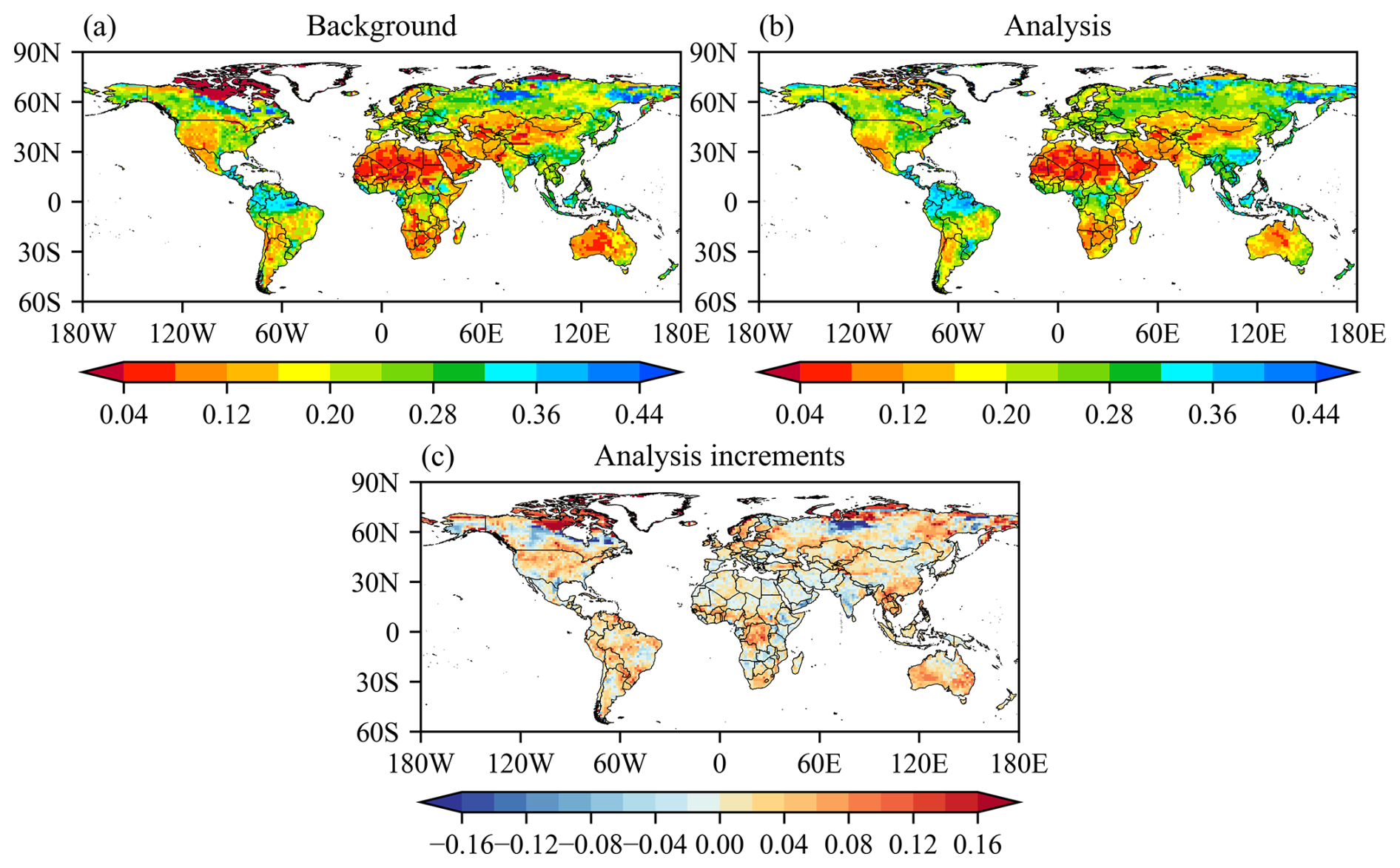
Figure 4 Spatial distribution of the instantaneous surface soil moisture at 06:00 UTC on 2 June 2022. (a) Background field; (b) Analysis field; (c) Analysis increment.

Figure 3 shows the estimated background error for the first mode based on curvelet transform. Figure 3a displays the spatial distribution of the global soil moisture background field, consistent with Fig. 1a, serving as the reference for subsequent error analysis. Figure 3b shows the difference between the original background field and the reconstructed field obtained through first-mode curvelet inverse transformation after adding error perturbations to the background field. The difference field exhibits distinct regional patterns. In transition zones with steep soil moisture gradients, such as western Sahara and northern Arabian Peninsula, Fig. 3b shows notably large errors. Eastern China, characterized by plains with relatively uniform soil moisture, displays smaller errors in Fig. 3b. This spatial pattern reflects the error structures are closely related to background field characteristics. This demonstrates that the curvelet transform, through its multiscale decomposition capability, enables background errors to preserve structural features during the transformation from physical space to spectral space.

3.4 Experiment Design

This study focuses on global simulation applications using CoLM with a spatial resolution of 1.4° × 1.4°. Regions with strong land-atmosphere coupling include the Amazon Basin, Sahel transition zone, Tibetan Plateau, and North American Great Plains (Barton et al., 2025; Koster et al., 2004; Seneviratne et al., 2010), where soil moisture variations serve as important signals for climate prediction. Among these regions, arid and semi-arid areas exhibit complex terrain and strong spatial heterogeneity in soil moisture, with surface energy and water budgets playing crucial feedback roles in the global climate system.

The assimilation period runs from 2 June to 1 August 2022, followed by a simulation period from 1 to 31 August 2022. Two experiments are designed. The first experiment employs the image assimilation method for soil moisture data assimilation (DA), conducting assimilation four times daily at 6 h intervals (00:00, 06:00, 12:00, and 18:00 UTC), assimilating only the GLDAS 0–10 cm surface soil moisture data. The second experiment serves as a control run (CTL) without data assimilation, running continuously from 2 June to 31 August 2022.

Regarding data preprocessing, considering that GLDAS soil moisture products have undergone rigorous quality control procedures, this study does not apply additional quality control to GLDAS data. For bias correction, we choose not to perform traditional bias correction because the primary purpose of image assimilation is to improve spatial structure characteristics of the background field. Bias correction processes statistically adjust the numerical distribution of observation fields, which can unavoidably affect or even distort the authentic spatial structure information contained in the observations (Shen et al., 2024; Wang and Tian, 2024; Zhou et al., 2020).

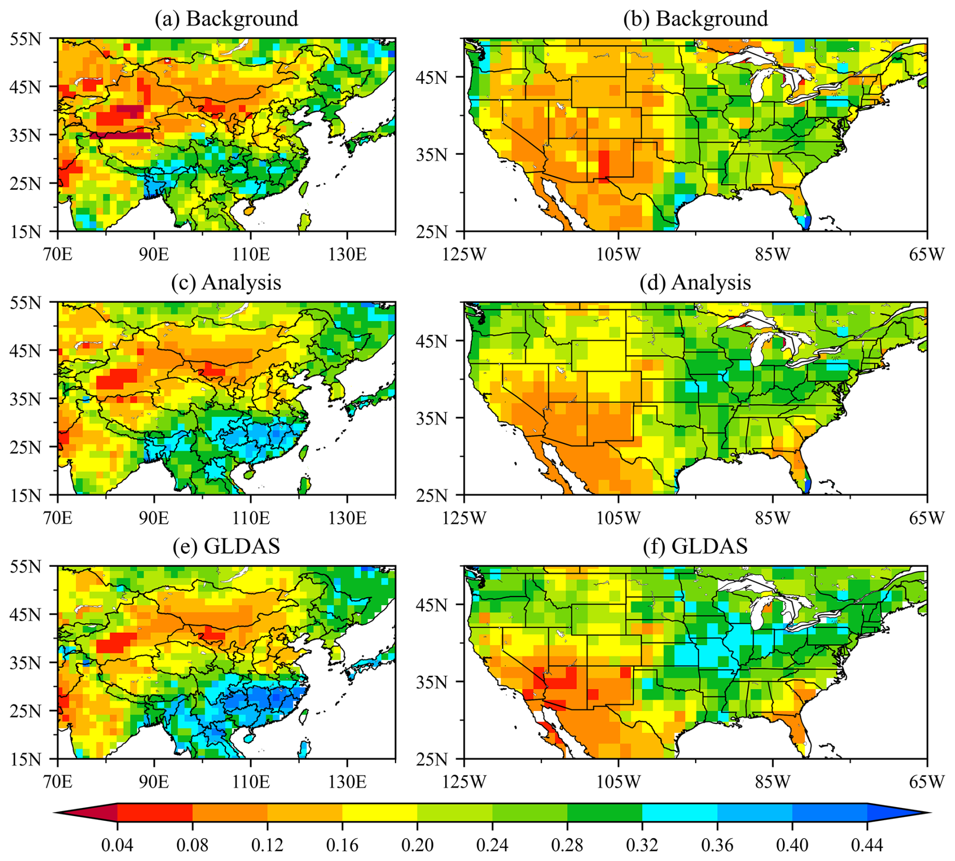
Figure 5 Spatial distribution of the instantaneous surface soil moisture over two typical terrain regions at 06:00 UTC on 2 June 2022. Panels (a) and (b) show the background field, (c) and (d) show the analysis field, and (e) and (f) show the GLDAS reanalysis data.

4 Results

4.1 Improvements in Soil Moisture Spatial Characteristics

The study first verifies the assimilation experiments to assess the effectiveness of the soil moisture image assimilation system. Figure 4 presents the spatial characteristics of the background and analysis fields for surface soil moisture at 06:00 UTC on 2 June 2022. As shown in Fig. 4a, tropical rainforest regions that include the Amazon Basin, the Congo Basin, and Southeast Asia generally exhibit values above 0.36 m³ m⁻³. Arid and semi-arid regions that comprise the Sahara Desert, the Arabian Peninsula, central Australia, and the Atacama Desert show values below 0.12 m³ m⁻³. Midlatitude temperate zones fall between 0.20 and 0.28 m³ m⁻³. This arrangement accords with global patterns of precipitation and evapotranspiration. The analysis field in Fig. 4b preserves the background structures across most areas, yet within continental interiors it introduces clear adjustments at multiple scales. The analysis increment in Fig. 4c indicates that the improvements from image assimilation arise chiefly in two types of regions. One consists of extensive plains such as the North American Great Plains, the East European Plain, and the outer margins of the West Siberian Plain. The other includes areas near major high terrain, for example the eastern slopes of the Rocky Mountains, the western flanks of the Andes, and the northern edge of the Tibetan Plateau. Because terrain effects amplify structural model errors in these transition belts, sizable assimilation increments emerge. More specifically, positive increments are concentrated over the central North American plains and the temperate grasslands of Eurasia, whereas negative increments appear in eastern Canada and along the northern boundary of the Brazilian Highlands.

To examine the fine-scale features of the image assimilation effect, Fig. 5 presents soil moisture before and after assimilation for two representative regions, the United States and China, together with GLDAS fields at the same time for comparison. As shown in the left column of Fig. 5, over China the background field indicates extensive aridity across the northwest under strong topographic influence. This dry zone connects directly to the Central Asian arid belt and lacks a clear transitional humidity gradient. Meanwhile, wetter conditions in the background concentrate near the boundary between Guangdong and Guangxi. The GLDAS data likewise display a pronounced soil moisture transition zone along the northwestern border of China and high soil moisture over the middle and lower reaches of the Yangtze River, consistent with Meiyu-season rainfall. After image assimilation, the analysis field reproduces both the northwestern transition belt and the humid Yangtze region well, and its spatial pattern agrees closely with GLDAS. In terms of magnitude, the analysis lifts the background's underestimated soil moisture in the northwestern transition zone from about 0.12 to roughly 0.20 m³ m⁻³, close to GLDAS, and it increases the Yangtze Basin maximum from 0.32 m³ m⁻³ in the background to nearly 0.40 m³ m⁻³, approaching the GLDAS value.

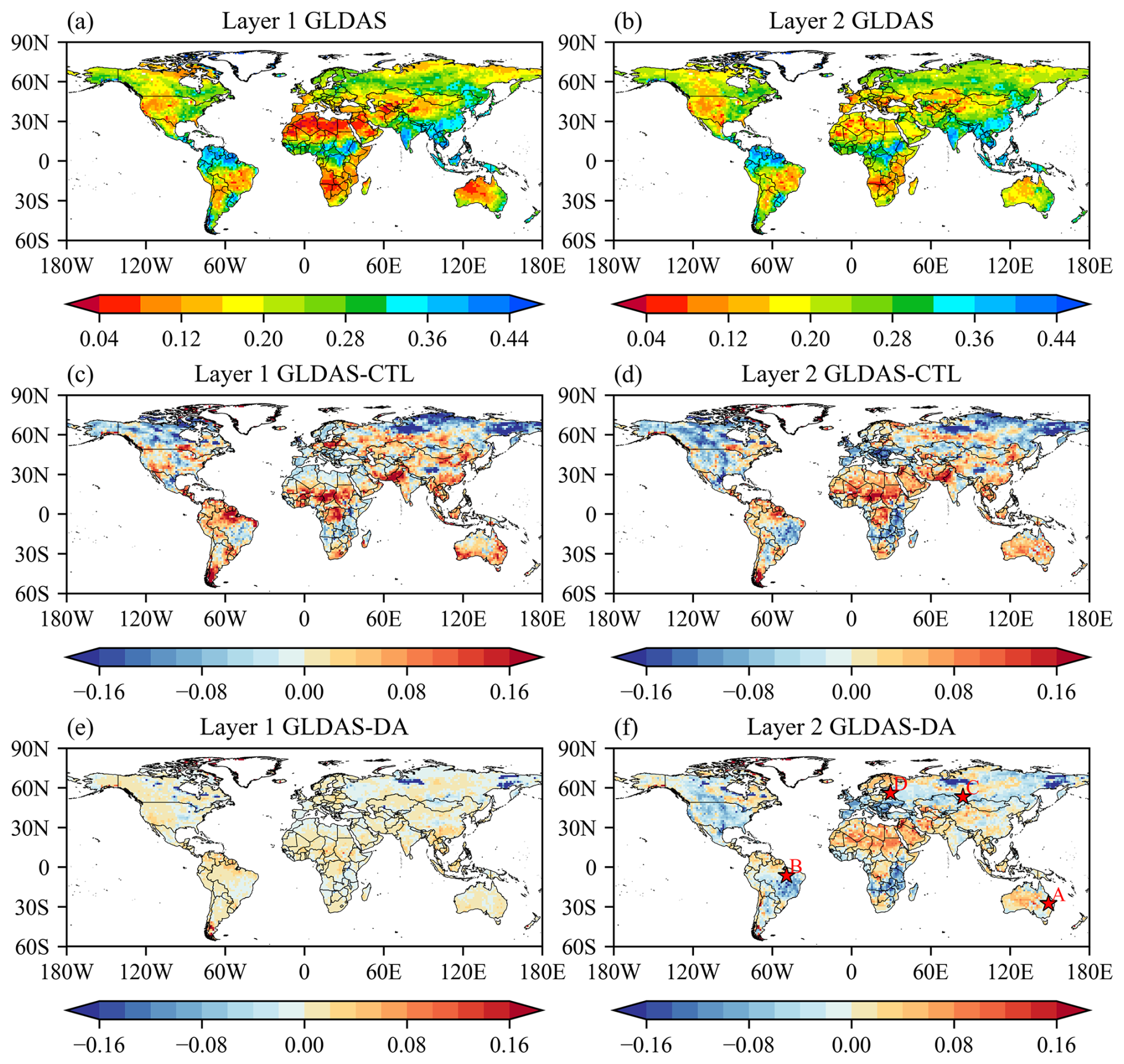
Figure 6 Spatial distribution of the instantaneous soil moisture at 00:00 UTC on 1 August 2022. Panels (a) and (b) show the GLDAS reanalysis data for the 0–10 cm surface layer and the 10–40 cm subsurface layer. Panels (c) and (d) show the differences between GLDAS and the CTL experiment for the two layers. Panels (e) and (f) show the differences between GLDAS and the image assimilation experiment. The pentagons in panel (f) mark the locations of typical vegetation types selected for further analysis.

In the United States region, the background field indicates widespread dryness across the western domain, particularly along the Cordillera mountain ranges, and relatively higher soil moisture levels appear in the central and eastern plains. The GLDAS dataset presents more detailed spatial patterns. In the west, soil moisture gradually decreases from north to south. In the east, it decreases outward from the central moist zone of the Great Plains. The analysis field reproduces these spatial features, including the north-to-south drying gradient in the west and the concentrated wet zone in the east. The spatial agreement between the analysis field and the GLDAS reference is generally consistent. In terms of magnitude, the assimilation system adjusts the underestimated soil moisture in both the northern mountainous regions in the west, where values increase from approximately 0.12 to about 0.20 m³ m⁻³, and in parts of the eastern plains, where values increase from around 0.24 m³ m⁻³ to nearly 0.32 m³ m⁻³. These adjustments reduce the discrepancies between the analysis and the GLDAS reference. The results suggest that the image-based assimilation system based on the curvelet transform improves the spatial representation of soil moisture. The analysis field better reflects multiscale spatial patterns that are consistent with independent observations.

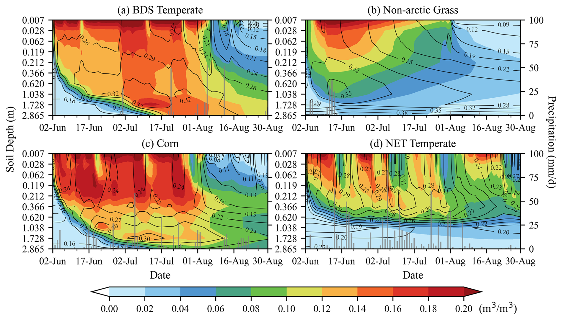
Figure 7 Temporal evolution of soil moisture differences between the image assimilation experiment and the CTL experiment (shading), along with the soil moisture profiles from the assimilation experiment (contours), for different vegetation types. Gray bars indicate precipitation. The locations correspond to the red pentagon markers in panel 6f.

4.2 Evaluation of Assimilation Performance

4.2.1 Evaluation of Assimilation Performance Using GLDAS Data

To evaluate the effects of the assimilation system during a continuous assimilation cycle and its impact on soil moisture at different depths, Fig. 6 presents the difference between the assimilated fields and GLDAS data at 00:00 UTC on 1 August 2022, following two months of continuous assimilation. Figure 6a and b show the GLDAS reanalysis data for soil moisture in the 0–10 cm surface layer and the 10–40 cm subsurface layer, respectively. In the surface layer, soil moisture exceeds 0.32 m³ m⁻³ in tropical rainforest regions, while it falls below 0.12 m³ m⁻³ in arid regions such as the Sahara Desert, the Arabian Peninsula, central Australia, and the Atacama Desert. In the subsurface layer, soil is wetter in arid regions because it is less directly affected by evapotranspiration. Figure 6c and d display the differences between the CTL experiment and the GLDAS data for the two layers. At the surface, the CTL field is systematically drier, with deficits in tropical humid regions reaching about 0.16 m³ m⁻³. In the subsurface, positive departures appear over Europe and the western United States. Figure 6e and f present the differences between the image assimilation experiment and GLDAS. Relative to CTL, the assimilation experiment reduces the discrepancies in both layers. In the surface layer, the magnitude of the negative bias decreases from 0.16 m³ m⁻³ in the CTL experiment to approximately 0.04 m³ m⁻³. In the subsurface layer, both the positive and negative bias extremes are also reduced. These results suggest that by improving the surface soil moisture field, the assimilation system contributes to better simulation of deeper soil moisture through hydrological processes in the LSM, such as gravitational drainage and capillary rise. However, large differences remain in certain regions such as Europe. These may be attributed to complex terrain, heterogeneous soil properties, or limitations in the LSM parameterizations, which require further investigation.

Although image-based assimilation directly adjusts surface soil moisture, anomalies in deep soil moisture are the dominant factor enabling soil moisture to continuously influence subsequent weather and climate variability. To further clarify the impact of image assimilation on deep soil moisture, Fig. 7 presents vertical–temporal cross sections of soil moisture differences (DA minus CTL) at model grid points corresponding to four representative vegetation types. These grid locations are marked by red pentagons in Fig. 6f and correspond to Broadleaf deciduous temperate shrub (BDS Temperate), Non-arctic grass (Non-arctic Grass), Corn (Corn), and Needleleaf evergreen temperate tree (NET Temperate). These points represent the locations where the assimilation-induced changes are most evident under each vegetation type.

Figure 7a shows the assimilation response for the BDS Temperate site. In this low-stature vegetation region, strong positive analysis increments are evident in the upper soil layer. During mid to late June, increments larger than 0.14 m³ m⁻³ are concentrated within the top 7 cm. The assimilation signal descends quickly through the profile, reaching 50 cm in roughly 5 d and 1 m by about day ten. Rainfall on 2 and 12 July accelerates this downward transfer of moisture anomalies. After assimilation ceases on 1 August, increments wane, yet the influence lingers in deeper layers for more than a month.

Figure 7b shows the Non-arctic Grass site. In contrast with BDS Temperate, the vertical response is more even and faster. The effect attains 1 m within about 5 d, then gradually weakens with depth. Once assimilation ends, a delayed signal persists between 0.62 and 1.04 m, where positive increments of 0.02 to 0.04 m³ m⁻³ remain. Figure 7c reports the Corn site. As with BDS Temperate, the signal reaches 50 cm within 5 d and 1 m by day ten. The surface perturbation then propagates downward to form a relatively uniform, high-increment zone above 36 cm, with values that stay nearly steady over time. Figure 7d summarizes the NET Temperate site. Vertical transmission is slower than in the other vegetation types, requiring around 155 d to reach 1 m. Beneath 1 m, the signal continues to penetrate and arrives near 1.73 m by late July. Even after assimilation stops, soil moisture differences continue to grow at greater depths. This delayed response suggests a strong memory effect in forest ecosystems, which may be linked to deep root water redistribution processes (Rahmati et al., 2024; Wei et al., 2006).

The more rapid propagation at the Non-arctic Grass and Corn sites is likely related to the shallower effective rooting depth of low-stature vegetation. In a Richards-equation-based matrix-flow framework, positive surface increments raise soil moisture and local hydraulic conductivity, favoring downward redistribution and percolation. After the anomaly moves below the main root zone, the constraint from root water uptake becomes weaker, and the signal can continue downward through gravity drainage and matric-potential gradients (Zeng, 2001). At the NET Temperate site, the slower but more persistent deep-layer response is consistent with the deeper rooting profile of forest ecosystems and the longer memory of soil moisture in the deeper root zone. Deep roots interact with a broader soil column through sustained water uptake, which can slow the downward transfer of assimilation increments while maintaining their influence at depth. The current CoLM2014 configuration, however, does not explicitly represent macropore preferential flow. Simulated downward propagation, particularly in forested or structurally heterogeneous soils, may therefore be smoother and slower than actual field responses when preferential flow is active (Beven and Germann, 2013; Fatichi et al., 2020).

These results indicate that although the image-based assimilation system directly adjusts surface soil moisture, its effects can gradually penetrate into deeper layers through continued model integration. The impact persists for more than a month after assimilation stops. This implies that soil moisture assimilation may not only influence short-term weather processes but also contribute to variability in near-term climate conditions. While the current results are based on offline simulations, applying the image assimilation system within a coupled land–atmosphere model would further amplify the impact of land surface assimilation through land–atmosphere feedbacks. This could allow soil moisture anomalies to persist for longer periods, thereby enhancing the predictability of short-term climate variability on extended timescales. This will be an important focus of our future work.

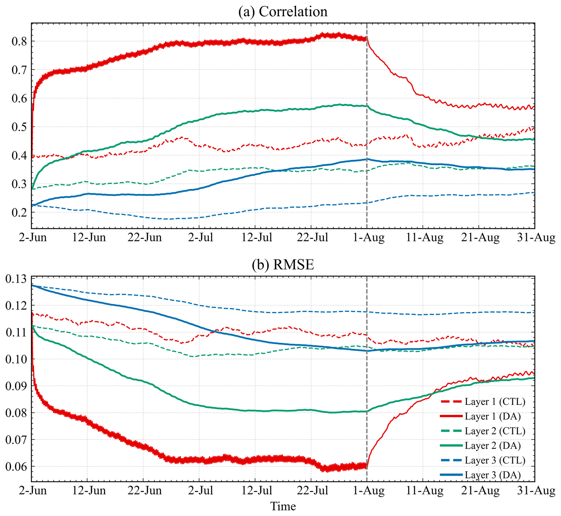
Figure 8 Three-hourly variations in SCC (a) and ubRMSE (b) between the assimilation experiment (solid lines) and CTL experiment (dashed lines) relative to GLDAS data from 2 June to 30 August 2022. Red lines represent the surface layer (0–10 cm), green lines the subsurface layer (10–40 cm), and blue lines the deep layer (40–100 cm). The vertical dashed line separates the assimilation period (left) from the forecasting period (right).

Figure 8 presents the evolution of spatial correlation coefficient (SCC) and unbiased root mean square error (ubRMSE) between the experiments (CTL and image-based assimilation) and the reference GLDAS dataset, computed every 3 h from 2 June to 30 August 2022. As shown in Fig. 8a, for surface soil moisture, the SCC rapidly increases from an initial value of approximately 0.4 to around 0.7 after the start of assimilation, indicating that the image assimilation system can quickly and effectively adjust the spatial structure of soil moisture. Throughout the assimilation period (2 June–1 August), the SCC of the assimilation experiment remains stably high between 0.75 and 0.80, significantly outperforming the CTL experiment (0.40–0.45). Similar improvements are observed for the subsurface and deep layers, although the enhancement is weaker in magnitude. For subsurface soil moisture, SCC increases from 0.35 in CTL to approximately 0.55 in the assimilation run, while for the deep layer, it increases from 0.25 to 0.35–0.40. This vertical gradient in improvement reflects the downward propagation of assimilation-induced corrections through model integration. Notably, after 2 July, while the SCC in the surface layer remains relatively stable, the SCC in the deeper layers continues to increase. During the forecast phase, the assimilation experiment still outperforms CTL, although the advantage gradually diminishes over time. The SCC of surface soil moisture decreases from 0.82 to 0.58, yet it remains consistently higher than that of the CTL experiment, suggesting that the positive impact of assimilation persists into the forecast period and provides improved initial conditions for medium-range predictions.

As shown in Fig. 8b, the temporal evolution of ubRMSE demonstrates that the image-based assimilation significantly reduces the simulation errors. For the surface layer, ubRMSE drops immediately from 0.118 to 0.095 m³ m⁻³ after the onset of assimilation and remains between 0.060 and 0.065 m³ m⁻³ during the entire assimilation window. Although improvements in the subsurface and deep layers are more modest, they show a consistent decreasing trend. The subsurface ubRMSE decreases from 0.110 to 0.080 m³ m⁻³, while the deep layer error reduces from 0.125 to 0.105 m³ m⁻³. During the forecast period, the assimilation error slightly increases but remains substantially lower than CTL. For instance, at the end of the one-month forecast, the surface ubRMSE increases to 0.095 m³ m⁻³ but still remains below the CTL level of 0.108 m³ m⁻³.

4.2.2 Evaluation of Assimilation Performance Using In-Situ Data

The preceding analysis is based on comparisons between the analysis field and reference data. Therefore, it does not constitute an independent validation but rather serves to assess the capability of the assimilation system in effectively incorporating structural information from observations. To objectively evaluate the performance of the image-based assimilation, independent in situ measurements are further employed. Considering the spatial coverage of the site data, two regions with relatively dense station distribution are selected: China (15–55° N, 70–140° E) and the continental United States (25–50° N, 125–65° W).

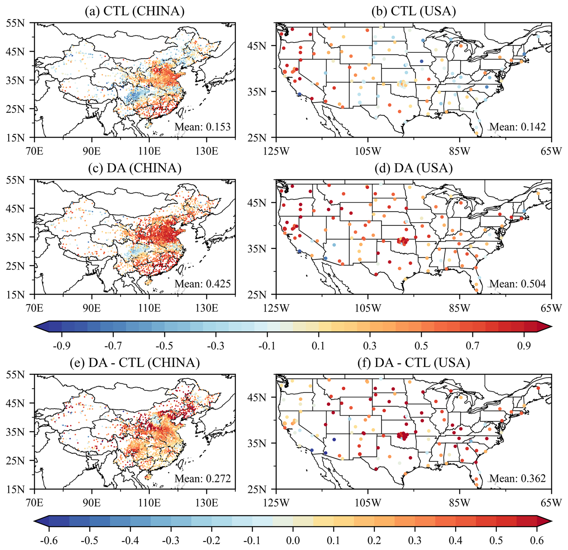
Figure 9 Spatial distribution of correlation coefficients between 10 cm soil moisture from in-situ data and model simulations during the assimilation period. Panels (a) and (b) show results from the CTL experiment over the China and United States domains. Panels (c) and (d) show results from the image assimilation experiment over the same regions. Panels (e) and (f) present the differences between the image assimilation and CTL experiments. The average correlation coefficient is provided in the lower-right corner of each panel.

Figure 9 presents the spatial distributions of correlation coefficients between simulated soil moisture and in situ observations for the CTL and assimilation experiments, as well as the corresponding differences between the two experiments across the two selected regions. In China (Fig. 9a), the CTL experiment shows the highest correlations along the southern coastal areas, with values ranging from 0.7 to 0.9. Moderate positive correlations (0.3–0.5) are found over the North China Plain and northeastern regions. In contrast, negative correlations below −0.3 are observed in the western region, particularly over the eastern Tibetan Plateau and Sichuan Basin. The regional mean correlation coefficient is 0.15. In the United States (Fig. 9b), the CTL experiment exhibits relatively strong positive correlations in the western region, with values exceeding 0.8 at some sites. However, over the central United States, most sites show weak or even negative correlations, yielding a regional average of 0.14. The image-based assimilation improves the simulation skill (Fig. 9c and d). In China, most sites exhibit positive correlations after assimilation. The North China Plain, northeastern China, and the southern region all reach values of 0.7–0.9. The western region, including the Sichuan Basin, shows clear improvement, with previously negative correlations becoming weakly negative or even positive. The regional average increases from 0.153 to 0.425. The improvement is more pronounced in the United States, where most sites shift from negative or weak correlations to moderate or strong positive correlations. In particular, many high-correlation sites (> 0.7) appear across the central United States. The regional mean correlation increases from 0.142 to 0.504. Figure 9e and f display the differences in correlation coefficients, providing a clear visualization of assimilation-induced improvements. In China, improvements are concentrated in the northern region, with increases of 0.3–0.4 over the North China Plain and northeastern China. The western region also shows improvements exceeding 0.3, with a mean increase of 0.272. In the United States, enhancements are more substantial. The central and eastern parts show widespread improvements of 0.4–0.6, and several stations experience increases greater than 0.6. The mean improvement reaches 0.362.

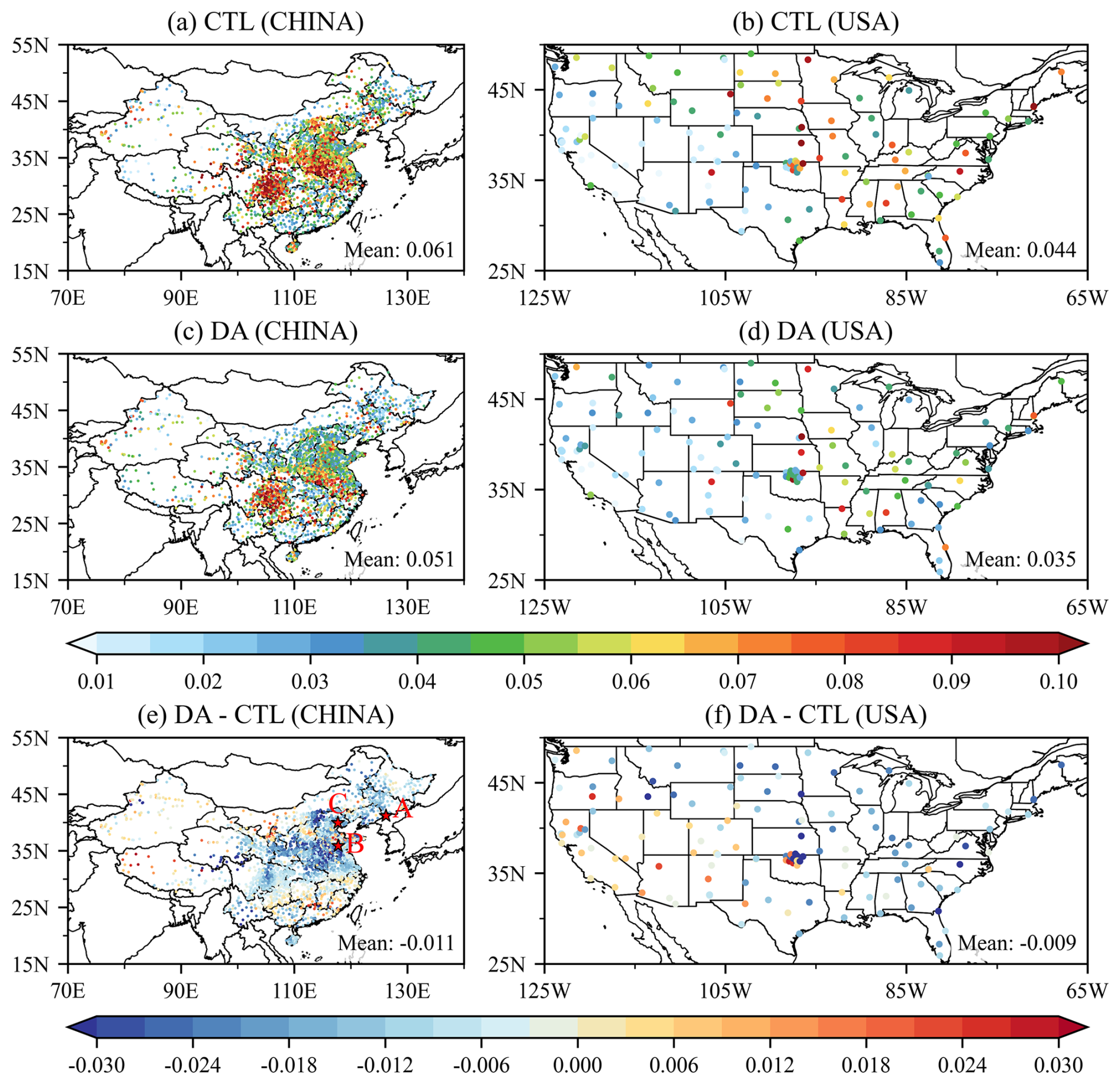
Figure 10 Spatial distribution of ubRMSE between 10 cm soil moisture from in-situ data and model simulations during the assimilation period. Panels (a) and (b) show results from the CTL experiment over the China and United States domains. Panels (c) and (d) show results from the image assimilation experiment over the same regions. Panels (e) and (f) present the differences between the image assimilation and CTL experiments. The average ubRMSE is provided in the lower-right corner of each panel. Red pentagons in panel (e) indicate the locations of typical vegetation-type stations.

Figure 10 shows the spatial distribution of ubRMSE between simulated and in situ soil moisture for the CTL and image assimilation experiments, along with the differences in ubRMSE. In the China domain (Fig. 10a), most ubRMSE values in the CTL experiment are below 0.05 m³ m⁻³, although relatively large errors exceeding 0.07 m³ m⁻³ appear in the North China Plain and Sichuan Basin. The domain-averaged ubRMSE is 0.061 m³ m⁻³. In the United States domain (Fig. 10b), the spatial distribution of ubRMSE resembles that of the correlation coefficient, with a gradual increase from west to east. Most sites show ubRMSE values below 0.04 m³ m⁻³, while only a few exceed 0.07 m³ m⁻³. The domain-averaged ubRMSE is 0.044 m³ m⁻³. The image assimilation experiment effectively reduces simulation errors (Fig. 10c and d). In the China domain, most ubRMSE values drop below 0.04 m³ m⁻³. Notably, the North China Plain and Sichuan Basin, which originally showed higher errors, experience substantial improvements. The domain-averaged ubRMSE is reduced from 0.061 to 0.051 m³ m⁻³. In the United States domain, the ubRMSE also decreases, with more stations showing values below 0.03 m³ m⁻³. The domain average decreases from 0.044 to 0.035 m³ m⁻³. These results indicate that the image assimilation system improves not only the correlation between model simulations and observations, but also reduces simulation errors. The enhanced correlation and decreased ubRMSE provide consistent evidence of the effectiveness of the image assimilation system.

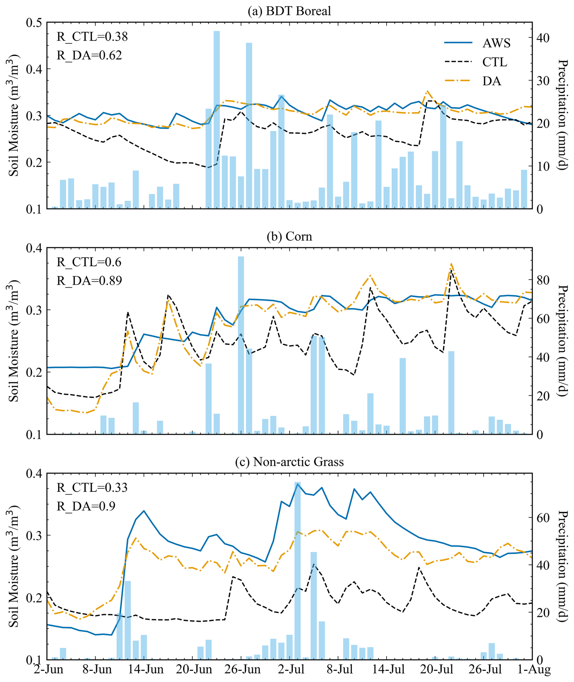
Figure 11 Time series of 10 cm soil moisture at representative in-situ stations during the assimilation period (2 June to 1 August 2022). Station locations are indicated by red pentagons in Fig. 10e. Black lines represent the CTL experiment, yellow lines indicate the image assimilation experiment, blue lines show in-situ observations at 10 cm depth, and blue bars represent precipitation. Correlation coefficients between each experiment and the in-situ observations are provided in the top-left corner of each panel.

Figure 11 presents the time series of 10 cm soil moisture at three representative in-situ stations from 2 June to 1 August 2022. These sites are located within different vegetation types, as marked by the red pentagons in Fig. 10e. The first station, located in a Broadleaf deciduous boreal tree (BDT Boreal) region, shows a correlation coefficient of 0.38 between the CTL experiment and observations, indicating limited agreement. During several rain events from late June into early July, the CTL experiment fails to reproduce the observed temporal swings in soil moisture, whereas the image assimilation experiment lifts the correlation to 0.62. Through the rainy period, assimilated soil moisture remains close to 0.3 m³ m⁻³ and aligns with the measurements, while the CTL simulation underestimates the moisture state. At the Corn site the gains are stronger. The correlation rises from 0.60 under CTL to 0.89 with assimilation, and the seasonal trajectory is captured, with soil moisture climbing from about 0.15 m³ m⁻³ in early June to roughly 0.32 m³ m⁻³ by late July. There are brief spikes on 11 June and 13 July that likely reflect inconsistencies in external forcing inconsistencies. For the Non-arctic Grass site the improvement is likewise substantial. The correlation coefficient increases from 0.33 in CTL to 0.90 with assimilation. The CTL simulation remains within a narrow range of 0.17–0.25 m³ m⁻³ at the site. In contrast, the image assimilation experiment captures both the magnitude and timing of soil moisture variability. Peak conditions in mid-June and early July are well represented, followed by a gradual drying, consistent with the rapid wetting and recovery behavior typical of grassland systems under precipitation forcing.

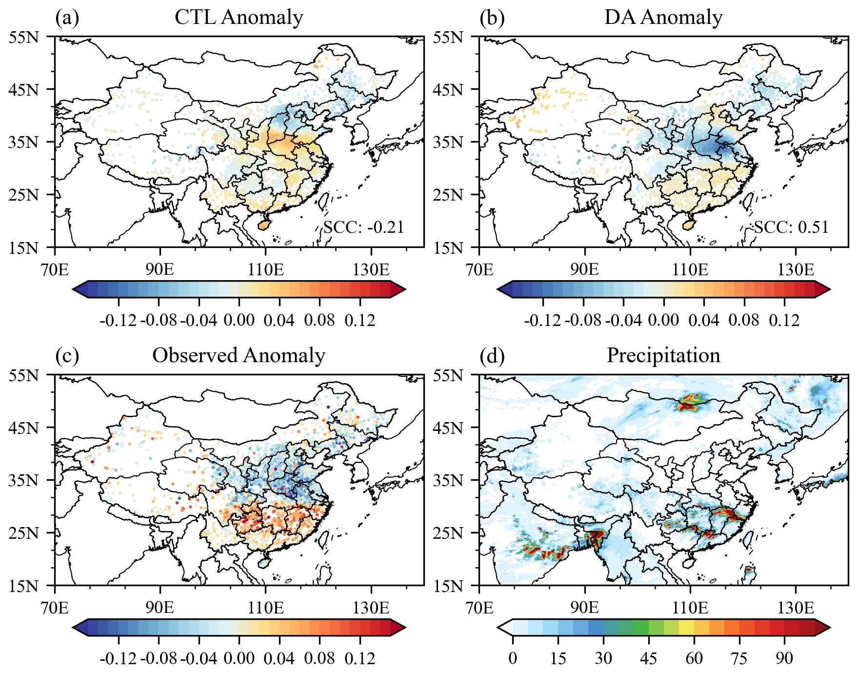
Figure 12 Spatial distribution of soil moisture anomalies on 18 June 2022, from (a) the CTL experiment, (b) the image assimilation experiment, and (c) in-situ observations. Panel (d) shows precipitation on the same date.

Figure 12 shows the spatial distribution of soil moisture anomalies on 18 June 2022, with anomalies defined as the difference between the daily values and the mean values over the assimilation period. On this day, intense precipitation events occurred over parts of southern China. A bilinear interpolation method was applied to interpolate the gridded model simulations to the locations of in-situ stations to enable a spatially consistent comparison with observations. Over northern China, particularly the North China Plain, in-situ observations indicate a clear pattern of negative anomalies, suggesting that soil moisture was lower than the mean state during the assimilation period. This condition is associated with persistent drought in the region, which is further supported by the precipitation data (Fig. 12d), showing reduced rainfall over this area. The image assimilation experiment (Fig. 12b) successfully captured this negative anomaly pattern, whereas the CTL experiment (Fig. 12a) produced positive anomalies. In contrast, over southern China, the CTL experiment shows localized positive anomalies (e.g., in Jiangxi Province), with slightly negative anomalies in surrounding regions. The image assimilation experiment exhibits a generally weak positive anomaly pattern. According to the precipitation observations, rainfall over southern China was relatively high on this day, consistent with the positive soil moisture anomalies recorded by the in-situ stations. Quantitative evaluation indicates that the spatial correlation coefficient between model simulations and in-situ observations increased from −0.21 in the CTL experiment to 0.51 in the image assimilation experiment, demonstrating improved representation of soil moisture anomalies.

5 Discussion and Conclusions

Due to the strong continuity of the atmosphere and the suppressing effect of the planetary boundary layer, the influence of soil moisture on the atmosphere typically requires coherent anomalies over a certain spatial scale. Only then can land–atmosphere interactions induce meaningful responses in the free atmosphere and lead to changes in mid-to-upper-level synoptic systems. This implies that the ability of LSMs to reproduce the spatial structures of soil moisture anomalies in the initial conditions is particularly critical for both weather and climate forecasting. However, because of the single-column architecture of land surface models, conventional land data assimilation methods generally emphasize point-wise corrections of soil moisture while neglecting improvements to its spatial structure.

To develop a more general image-based assimilation approach that aligns with land surface model characteristics, this study builds on previous work and proposes an EnKF-like image assimilation method based on the curvelet transform. By defining the curvelet transform as the operator linking the physical space and the spectral domain, the entire assimilation process is carried out in spectral space. The new assimilation system uses ensemble methods to dynamically estimate both background and observation error covariance. By assimilating curvelet coefficients in spectral space, the system achieves an optimal match between the analysis field and the structural features of the observational image, allowing simultaneous optimization of both spatial structure and magnitude in soil moisture analysis fields.

Evaluation results show that the proposed image assimilation method effectively improves the spatial representation of the soil moisture analysis fields. For surface soil moisture, the spatial correlation with GLDAS increases from 0.4 in the background to 0.8 after assimilation, while the error is reduced, with ubRMSE decreasing from 0.12 to 0.06 m³ m⁻³. Under the constraints of the model's dynamical and thermal processes, the spatial structure of deeper soil layers is also improved. The spatial correlation increases from 0.35 to 0.55 in the 10–40 cm layer, with errors reduced by 27 %, and from 0.25 to 0.4 in the 40–100 cm layer.

Independent validation with in-situ observations further confirms the effectiveness of the method. In China, the mean correlation between soil moisture and in-situ observations increases from 0.153 to 0.425, and ubRMSE decreases from 0.061 to 0.051 m³ m⁻³. Improvements are even more pronounced in the United States, where correlation increases from 0.142 to 0.504 and ubRMSE decreases from 0.044 to 0.035 m³ m⁻³. These quantitative assessments collectively demonstrate the effectiveness of the EnKF-like image assimilation method. It should be noted that the in-situ validation is affected by a point-to-grid scale mismatch. A single station may not fully represent the mean soil moisture condition of a 1.4° grid cell, particularly in heterogeneous or sparsely instrumented regions such as western China. Therefore, the correlation and ubRMSE values should be interpreted as indicators of temporal consistency with independent observations rather than exact point-scale accuracy. In particular, ubRMSE may include both retrieval/model errors and representativeness errors associated with spatial scaling.

Bias correction represents another source of uncertainty. A spatially uniform bias may have a limited impact on image-based assimilation because it does not substantially alter spatial patterns. Conversely, regionally varying systematic biases in observations can be incorrectly incorporated as spatial structures during assimilation, thus degrade assimilation performance. But because estimating such regional bias characteristics requires long-term observational records, and because this study focuses on evaluating the ability of image assimilation to capture and reconstruct spatial structures, systematic bias correction is not considered here. Future work will assess the impact of bias correction using long-term observational datasets.

Recent studies have increasingly demonstrated the potential of satellite data assimilation to improve high-resolution land surface and hydrological modeling by better constraining soil moisture, vegetation dynamics, and surface–groundwater interactions (Pinnington et al., 2021; Montaldo et al., 2022; Zafarmomen et al., 2024). Image assimilation may offer greater advantages in high-resolution land surface modeling applications. Owing to the exactness of the curvelet transform, the small-scale spatial heterogeneity associated with high-resolution modeling can be represented by curvelet modes. The ensemble-based error estimation approach can also translate representativeness errors into uncertainties of curvelet coefficients at the corresponding scales. Therefore, through the curvelet transform, image assimilation can identify and extract dominant physical signals in spectral space and apply targeted assimilation adjustments, thereby helping to preserve the accuracy of small-scale soil moisture features in high-resolution analysis fields.

Although the above analysis demonstrates the potential advantages of image assimilation in preserving spatial structures, a direct comparison with point-based assimilation methods would further clarify its relative strengths and limitations. However, a mature point-based assimilation system specifically applicable to CoLM is not yet available, making it difficult to objectively compare the performance differences between image-based and point-based assimilation at this stage. From a methodological perspective, the two are highly complementary. Image assimilation offers clear advantages in capturing spatial patterns and maintaining structural continuity, whereas point-based assimilation is more effective for assimilating high-accuracy in-situ observations and handling localized extreme anomalies. Therefore, future work will focus on developing hybrid assimilation strategies that apply scale-appropriate techniques at different spatial scales, fully leveraging the strengths of each method. For example, one potential implementation would be to use image assimilation to efficiently adjust the spatial structure of soil moisture in the background field, while also identifying regions with coherent change patterns. Conventional high-accuracy point-based assimilation could then be applied within these specific regions. This strategy would allow observational data to precisely constrain local states and anomalies without disrupting the large-scale structural continuity maintained by image assimilation, and may therefore provide a promising pathway for future hybrid assimilation.