BORIS-2 – a benthic ecosystem model based on allometry

We present a model describing the population dynamics of benthic biota, feeding from a common resource that is supplied by a flux of sinking organic carbon arriving on the seafloor. By using allometric relationships for the physiological processes of growth, mortality and respiration, and for food limitation, the model represents the population dynamics of organisms ranging in size from bacteria (10⁻¹⁴ g wet weight C) to large metazoans (10³ gwwt C). The effect of temperature on physiological rates is also included. The only forcing information required is the ambient temperature and the rate of supply of sinking organic carbon. The model can be used for, and tuned to, specific locations. However, a parameter set is provided that is generally applicable. The ability of the model to simultaneously reproduce biomass size distributions at five contrasting sites is demonstrated for this parameter set. Other examples of use are also shown, using the model to explore global patterns of benthic biomass, and responding to a change in food supply.

1 Introduction

The surface ocean, or epipelagic, ecosystem has received considerable attention from modellers for a variety of reasons, spanning from the magnitude of biogeochemical fluxes (e.g. Burd, 2024) and fundamental questions of ecosystem structure (e.g. Woodson et al., 2018) and biodiversity (e.g. O'Dor et al., 2009) to more societal issues such as fisheries management (e.g. Karp et al., 2023) and climate modelling (Kwiatkowski et al., 2020). However, the seafloor, or benthic, ecosystem has received much less attention, particularly in the deeper regions away from the continental shelves. This is despite the regions deeper than 1000 m constituting over half of the earth's surface area (Ramirez-Llodra et al., 2010; Harris et al., 2014).

The benthic ecosystem of the deep ocean (aside from hydrothermal vents) is almost entirely dependent on external input for food, with the majority in the form of organic material sinking down from the waters above. This means that the benthic ecosystem is susceptible to changes in production of this organic material that may occur several kilometres above it (Ruhl et al., 2008), such as in response to climate change (Yool et al., 2017). Benthic ecosystems are also subject to direct pressures such as trawling, dredging, oil and gas activities, and seabed mining. To understand and to predict the future for benthic ecosystems we therefore need models that adequately capture their response to such drivers, across the full ecosystem and over appropriate timescales.

Building models that capture the key interactions within an ecosystem is of value for three reasons: construction of a model forces us to identify the key processes and to articulate our understanding of them in a precise manner; the behaviour of the model allows us to identify gaps and uncertainties in that knowledge; and by linking the model to forecasts for how environmental drivers may change it allows us to make predictions for the fate of the ecosystem across different scenarios. One modelling strategy is to represent an ecosystem as different functional groups, particularly those linked to particular fluxes of interest into and out of the sediment e.g. deposit feeders and aerobic/anaerobic bacteria (e.g. Butenschön et al., 2016; Ehrnsten et al., 2018). This approach is valuable, for example, in studying the biogeochemistry of shelf systems where the interactions between sediment, overlying water and benthic ecosystem may need to be captured because the feedback on the overlying water column may be significant given the shallow depths. Shelf systems also benefit from a greater array of data to constrain a model as they are more accessible for sampling than deeper waters. More generally, a paucity of data to constrain a model or limited understanding of causal relationships are common hindrances, particularly for deep-sea ecosystems because of the remote and challenging nature of the environment being studied. For situations where the ecosystem can be approximated as unchanging in time, statistical methods have been used (e.g. Reiss et al., 2014), particularly for modelling distributions of groups or individual species, but also for distributions of biomass (Wei et al., 2010; Jones et al., 2014). For deep-sea ecosystems where data are sparser, an inverse approach has been used to estimate fluxes between functional and size category components of the ecosystem at equilibrium (Soetaert and van Oevelen, 2009; Durden et al., 2017; de Jonge et al., 2020), with the size classes mirroring those represented by typical benthic sampling techniques. However, behaviour such as switch-feeding (e.g. alternating between suspension feeding and predation) in deep-sea fauna (Durden et al., 2015; Iken et al., 2001) complicates the use of discrete functional groups based on feeding types (Durden et al., 2017).

Another approach, is to represent the community purely as a collection of different size classes of organisms (Kelly-Gerreyn et al., 2014; Blanchard et al., 2011; Laguionie Marchais et al., 2020) rather than as functional groups or species. As described below, this offers considerable simplification in model structure and parameterisation. Furthermore, by using allometric relations to base the model on the representation of rates, rather than stocks, this approach also allows the response of ecosystems with time to be tracked.

Considerable attention has been given to observations showing relationships which appear to scale in a consistent way with body size, both at a population (e.g. abundance – White et al., 2007) and an individual (e.g. physiological rates – Gillooly et al., 2001) level. This phenomenon has been widely observed, on land (e.g. Nagy, 1987), in the air (e.g. Niven and Scharlemann, 2005) and in the sea (e.g. Molony and Field, 1989) including the deep ocean (Durden et al., 2019; McClain et al., 2012; Mahaut et al., 1995). That such behaviour has been observed across many habitats and orders of magnitude in size of organism unsurprisingly led to a search for a “Universal” law explaining such behaviour. Metabolic rate controls ecological processes at individual and ecosystem levels by determining resource uptake and allocation. The Metabolic Theory of Ecology (MTE; West et al., 1997; Brown et al., 2004) asserts that, to first order, this rate is controlled by the size of organism and the ambient temperature. This provides a potential explanation for the existence of a power-law relationship between physiological rates and body size. However, there remains a discussion over the taxonomic or functional scale at which other features or processes might disrupt any universal scaling (Seibel and Drazen, 2007), the precise value of the scaling (Isaac and Carbone, 2010; Brey, 2010; Glazier, 2022) and the extent to which such an approach applies to systems that are not in equilibrium (McCarthy et al., 2019).

Notwithstanding these caveats, an allometric approach still has considerable value when applied at broad ecosystem scales. To support use of an allometric approach, we give just a few examples for three key processes: growth, respiration and mortality. Motivated by predictions of MTE, Ernest et al. (2003) successfully tested the predicted scaling exponent of −0.25 for growth rate, for organisms spanning 10⁻¹⁴–10⁸ g in size. More specific to this study, with a focus on macrobenthos, Cusson and Bourget (2005) brought together empirical relations from previous studies (their Table 8) that demonstrate similar evidence of scaling of growth rate with size. For respiration, Mahaut et al. (1995) found a power-law scaling with size for deep-sea organisms, spanning seven orders of magnitude. This was for a single location, however, so not suitable for testing a temperature dependence. For mortality, McCoy and Gillooly (2008, 2009) brought together estimates of natural mortality spanning 22 orders of magnitude including plants, fish, birds, mammals and invertebrates, finding that a power-law scaling with size plus an exponential dependence on temperature captures the dominant pattern. A restriction of their data purely to invertebrates found a similar result (McCoy and Gillooly, 2009), still spanning 11 orders of magnitude in size. Again, focussed on marine benthic organisms, McClain et al. (2012) analysed data for growth, respiration and turnover (which can be a proxy for mortality) and demonstrated a clear power-law scaling with size, with additional support for an exponential relationship with temperature. There are, therefore, reasonable grounds for adopting an allometric approach.

Kelly-Gerreyn et al. (2014) constructed a dynamic model for benthic organisms based on allometry such that physiological rates vary with body size (Benthic Organisms Resolved in Size – hereafter “BORIS-1”). BORIS-1 was capable of reproducing the size distribution of organisms at three sites contrasting in depth between 150m and 1600m. This model assumed that all organisms were detritivores, eating from a common pool of detritus supplied by organic material sinking to the seafloor, the particulate organic carbon (POC) flux. BORIS-1 demonstrated that an allometric model with a small number of physiological processes (ingestion, assimilation and respiration/mortality) that are common to all organisms but scale with body size can capture the size-distribution of biomass seen in observations. However, the model has several limitations. The first is that it only represents a limited range of sizes ($\mathrm{8.9}\times {\mathrm{10}}^{-\mathrm{7}}$ to $\mathrm{2.9}\times {\mathrm{10}}^{-\mathrm{2}}$ g wet weight). It was therefore necessary to assume a specific fraction of POC flux that was consumed and respired by organisms not represented by the model, and hence not available to the modelled organisms. The omitted organisms included both smallest (e.g. bacteria) and largest (e.g. large sea cucumbers) size ranges. The physiological rates were also not dependent on temperature even though there is evidence that physiological rates typically increase as the environment warms (e.g. Gillooly et al., 2001). Additionally, the mortality rate had a dependency on the POC flux in BORIS-1. This resulted in estimates of longevity that unrealistically varied across several orders of magnitude for the same organism at different locations.

This paper presents an expanded and updated version of BORIS-1 that addresses these limitations. The resulting model, BORIS-2, spans the full range of organism sizes, includes the physiological role of temperature, and is parameterised using a larger dataset that includes observations from a greater range of sites with contrasting environmental conditions, including the abyssal ocean. A single parameter set that allows the model to capture the ecosystem structure across these sites is given and examples are demonstrated for how the model may be used to study both local and global questions. It is worth stressing that the aim of BORIS-2 is to capture broad ecosystem behaviour, i.e. macroecology, across the full range of body sizes, not to capture the dynamics of specific species.

2 BORIS-2 model description

BORIS-2 represents benthic organisms spanning in size from bacteria to large metazoans (Fig. 1). It does so by dividing benthic organisms into size classes and using an allometric approach. The size classes are defined on the basis of individual wet weight body mass (units: grams wet weight – g wwt). From the smallest to the largest, each size class spans twice the range of the former. More specifically, the mean body mass of organisms within a size class spans from $\mathrm{1.3}\times {\mathrm{10}}^{-\mathrm{14}}$ g wwt (13 fg) for the smallest to 3.6×10³ g wwt (3.6 kg) for the largest. The lower limit of the smallest class is $\mathrm{0.88}\times {\mathrm{10}}^{-\mathrm{14}}$ g wwt (9 fg) and the upper limit of the largest is 5.1×10³ g wwt (5.1 kg). The size classes are chosen to be consistent with those used for size-spectra biomass data (e.g. Laguionie Marchais et al., 2020) and BORIS-1 (Kelly-Gerreyn et al., 2014). The smallest size class is based on the smallest observed bacteria (Luef et al., 2015), using a conversion from g C to g wwt of 11.5 (Brey, 2010). The largest size class is chosen to be broadly representative of benthic habitats. It is consistent with a detailed assessment of invertebrates for a well-studied abyssal site, the Porcupine Abyssal Plain (one of the sites described in Sect. 2.5). These upper and lower biomass limits, together with the factor of two scaling used between biomass size classes, sets the number of model size classes to 59. For application of BORIS-2 to specific locations where larger organisms are known, the upper size limit is easily changed. The BORIS-2 size range currently spans over 18 orders of magnitude.

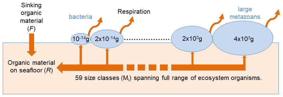
Figure 1 Schematic of BORIS-2. Within each size class (M_i) the total biomass (B_i) is controlled by growth, using organic material on the seafloor, and losses to respiration and mortality. Organic material (R) accumulates on the seafloor from the deposition of sinking particulate organic carbon (F) and mortality of benthic organisms. Growth, respiration and mortality are all assumed to scale as a power-law with M_i and as an exponential function of ambient temperature (see Sect. 2). Numbers denote median mass (units: g wet weight) for each size class and example organisms of smallest and largest size classes are given in blue.

2.1 Ecological interactions

BORIS-2 comprises a set of differential equations describing the time-varying behaviour of N=59 size classes ingesting a common resource, R, that represents the stock of detrital food available to the benthic community (i.e., in / on the seafloor or in the benthic boundary layer). The model does not capture any direct predation or cannibalism, and instead represents a community of detritivorous heterotrophs. This decision is based on the different nature of benthic and pelagic ecosystems. Total biomass in a size range increases with body mass in benthic ecosystems (e.g. Benoist, 2020; Kelly-Gerreyn et al., 2014). In the pelagic ocean, biomass is roughly equal across different sizes (Hatton et al., 2021). The greater accumulation of biomass in larger organisms in the benthic system is consistent with a greater transfer efficiency arising from a reduced role of predation and a greater role of feeding from a common detrital resource. We effectively assume that the dominant influence on benthic ecosystems is having neighbours competing for your food, rather than eating you. This assumption is discussed in more detail in Sect. 4.1.

The total biomass represented by all organisms per square metre in each size class i of nominate mass M_i (units: grams wet weight – g wwt) is represented as B_i (units: g wwt m⁻²) which varies with time, t (units: d), according to the equation

$$\begin{array}{}\text{(1)}& {\displaystyle \frac{\mathrm{d}{B}_i}{\mathrm{d}t}}=\stackrel{\mathrm{gross}\mathrm{growth}}{\overbrace{g_i\cdot f\left(R,B_i\right)\cdot B_i}}-\stackrel{\mathrm{respiration}}{\overbrace{r_i\cdot B_i}}-\stackrel{\mathrm{mortality}}{\overbrace{m_i\cdot B_{-}}}\end{array}$$

where g_i is the maximum specific growth rate and r_i and m_i are the specific rates of respiration and mortality, respectively. All of g_i, r_i and m_i have units of 1 d⁻¹. The function f(R,B_i) represents how growth is limited by increasing population size and/or decreasing resource availability (see Sect. 2.2). The associated equation controlling the amount of resource, R (units: g wwt m⁻²), is

$$\begin{array}{}\text{(2)}& {\displaystyle \frac{\mathrm{d}R}{\mathrm{d}t}}=F-\sum _{i=\mathrm{1}}^N\left[\stackrel{\mathrm{gross}\mathrm{growth}}{\overbrace{g_i\cdot f\left(R,B_i\right)\cdot B_i}}-\stackrel{\mathrm{mortality}}{\overbrace{m_i\cdot B_{-}}}\right]\end{array}$$

where F is the POC flux to the seafloor through gravitational sinking of detritus (g wwt m⁻² d⁻¹). Note that at equilibrium the rate of supply of organic material, F, equals the respiration by the whole ecosystem, $\sum _{i=\mathrm{1}}^N{r}_i\cdot B_i$. It is assumed that the long-term burial of organic material in sediment is negligible compared to POC and total respiration fluxes. (Section 4.1 discusses how this assumption might be relaxed.) A linear mortality term, m_i⋅B_i, is used in BORIS-2. (The reason for using this rather than the quadratic ${\mathit{\mu }}_i\cdot B_i^{\mathrm{2}}$ parameterisation used in BORIS-1 is given in the Appendix.)

2.2 Growth limitation: food scarcity and interference

The growth limitation function, f(R,B_i), reflects the impact on growth arising from competition for limited resources. This function is chosen to capture two effects. First, low availability of food, R, should lead to a reduced rate of intake and growth. Second, any increase in the number of organisms (for which B_i is a proxy) looking for food should reduce the likelihood of any individual finding it, a phenomenon known as interference (e.g. DeAngelis et al., 1975). More specifically, we assume the parameterisation

$$\begin{array}{}\text{(3)}& f\left(R,B_i\right)=\mathrm{1}/\left(\mathrm{1}+a_i{B}_i/R\right).\end{array}$$

The parameter a_i is present to account for how interference may scale with size. For example, larger organisms can search a given area more quickly than a smaller one, in general, either because motility generally increases with size or more simply because they occupy a greater area. Note that a_i is unitless. The function f(R,B_i) varies between 0 and 1, with a value of zero entirely ceasing growth and a value of one leading to growth at the maximum rate, g_i. To demonstrate that the function has the required properties, first consider the case where food is very abundant such that R≫a_iB_i. Then $f(R,B_i)\sim \mathrm{1}$ and there is no limitation of growth. If resource is scarce such that R<a_iB_i, then $f(R,B_i)\sim R/\left(a_i{B}_i\right)$ which is always a value less than one but increases and decreases linearly with both resource, R, and abundance of organisms, represented by B_i. Note that for simplicity we currently only incorporate competition for resources within a size class. This is the simplest assumption given that different size classes seek food at different spatial scales. What is a meal for a bacterium is unlikely to be a meal for a holothurian. It would, however, be straightforward to include competition from other size classes simply by using a sum over those classes in the denominator. The form of the interference parameter, a_i, is discussed in the next section (Sect. 2.3). Figure 2 and Sect. 2.4 show further how the function f(R,B_i) varies, in particular demonstrating that it affects all size classes equally i.e. that it does not lead to some size classes being food limited while others are growing near maximum rates.

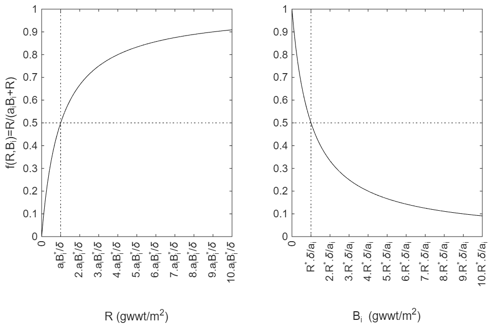
Figure 2 Plots showing how the growth limitation function, $f(R,B_i)=\mathrm{1}/(\mathrm{1}+a_i\cdot B_i/R)$ varies as either R (left panel) or B_i (right panel) is varied. R^* and $B_i^{*}$ denote values at steady state (vertical dotted line), where additionally $\mathit{\delta }\cdot R^{*}=a_i\cdot B_i^{*}$. Note that because of the scaling behaviour of a_i, a_i⋅B_iis the same for all i at any site.

2.3 Allometric and temperature influences

In BORIS-2 allometry is used to describe four physiological or physiologically affected processes across the range of body sizes. The physiological processes are growth (g_i), respiration (m_i) and mortality (r_i). The physiologically affected process is growth limitation, controlled by parameter a_i. All of these are assumed to be determined by size (body mass) and environmental temperature.

The effect of temperature is assumed to be identical for all four processes and represented by a function, θ(T), which is taken to be

$$\begin{array}{}\text{(4)}& \mathit{\theta }\left(T\right)=\exp [-E\cdot \mathit{\tau }/k]\end{array}$$

with

$$\begin{array}{}\text{(5)}& \mathit{\tau }=\mathrm{1}/\left(T+T_{\mathrm{abs}}\right)-\mathrm{1}/\left(T_{\mathrm{ref}}+T_{\mathrm{abs}}\right)\end{array}$$

where T is temperature (units: °C), T_ref (units: °C) is a reference temperature, T_abs=273.15 K converts T and T_ref to units of Kelvin (K), and k is Boltzmann's constant ($\mathrm{8.62}\times {\mathrm{10}}^{-\mathrm{5}}$ eV K⁻¹). This is a widely used formulation applied both in empirical studies (e.g. Brey, 2010) and papers developing ideas around the Metabolic Theory of Ecology (e.g. Gillooly et al., 2001). E (units: eV) is often described as an activation energy. We discuss the value chosen for E in Sect. 2.5. T_ref is chosen to be 20 °C. While this may seem an arbitrary choice of reference temperature, it has no impact on rates. Using a different T_ref simply requires a numerical change in parameters (g₀, r₀, m₀ and a₀) to compensate for the change.

It is assumed that the three physiological rates (g_i, m_i and r_i) scale with body size in an identical way. This is purely taking the option requiring fewest assumptions given the current uncertainty in how these rates vary with size. As the link between interference and physiology is more tentative, a_i is theoretically allowed to scale independently (but see Sect. 2.5). More specifically, growth, respiration and mortality have common scaling exponent β, whereas interference scales with exponent α:

$$\begin{array}{}\text{(6)}& {\displaystyle }& {\displaystyle }{g}_i=\mathit{\theta }\left(T\right)\cdot g_{\mathrm{0}}\cdot M^{\mathit{\beta }}\text{(7)}& {\displaystyle }& {\displaystyle }{r}_i=\mathit{\theta }\left(T\right)\cdot r_{\mathrm{0}}\cdot M^{\mathit{\beta }}\text{(8)}& {\displaystyle }& {\displaystyle }{m}_i=\mathit{\theta }\left(T\right)\cdot m_{\mathrm{0}}\cdot M^{\mathit{\beta }}\text{(9)}& {\displaystyle }& {\displaystyle }{a}_i=\mathit{\theta }\left(T\right)\cdot a_{\mathrm{0}}\cdot M^{\mathit{\alpha }}.\end{array}$$

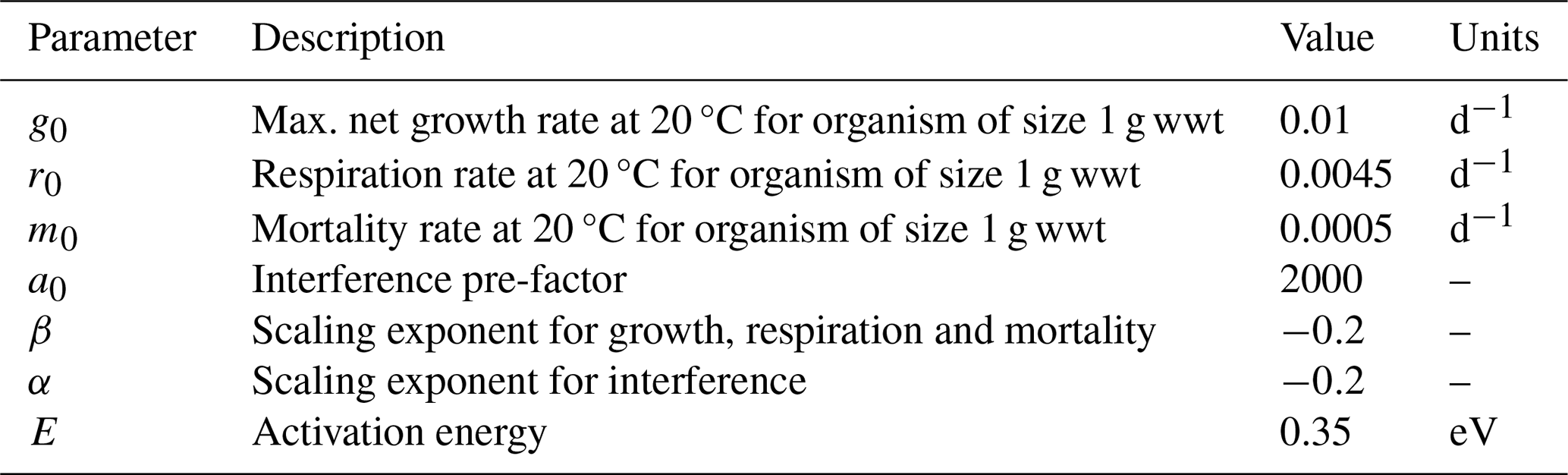
The values chosen for the seven parameters used in the model (g₀, r₀, m₀, a₀, α, β, E) are given in Sect. 2.5 (and Table 1), together with a description of the data used to constrain them. The performance of the model using this parameter set is then described in Sect. 2.6 and the uncertainties associated with their values are discussed in Sect. 2.7. Before then a steady state solution for the model is presented, both for its own use and as a source of useful information for constraining parameter values.

Table 1 Parameter set for BORIS-2.

2.4 Steady state solution

The model has a steady state solution which can be written in a simple form. This provides a means to initialise simulations, to validate dynamical model runs (if run to equilibrium) or to accelerate model runs where time-scales are longer than organism response times.

Indicating steady state values with an asterisk, the steady state solution is

$$\begin{array}{}\text{(10)}& {\displaystyle }& {\displaystyle }{R}^{*}={\displaystyle \frac{F}{\sum _{i=\mathrm{1}}^N\frac{r_i\cdot \left(g_i-r_i-m_i\right)}{a_i\cdot \left(r_i+m_i\right)}}}\text{(11)}& {\displaystyle }& {\displaystyle }{B}_i^{*}={\displaystyle \frac{\left(g_i-r_i-m_i\right)}{a_i\cdot \left(r_i+m_i\right)}}{R}^{*}.\end{array}$$

This steady state solution provides a few insights into the behaviour of the model. First, both resource, R, and biomass in all size classes, B_i, increase linearly with F. This is not surprising as we would expect abundance of detritus and biomass to increase with increasing food supply. Second, B_i scales with size with the same exponent, −α, as $\mathrm{1}/a_i$ (i.e. $B_i^{*}\propto M^{-\mathit{\alpha }}$). This is because g_i, r_i and m_i all scale the same with size, as mentioned above, and so the scaling of ($g_i-m_i-r_i$) in the numerator for $B_i^{*}$ is cancelled by the identical scaling of (r_i+m_i) in the denominator. Hence, the biomass spectral slope is effectively set by interference. Although this might be unexpected it should be noted that the processes contributing to a_i are still very poorly known and its scaling is likely to be influenced by physiological processes, such as respiration associated with enhanced movement for example. The theoretical model of Damuth (2007) is potentially relevant here as it links competition for resources to allometric scaling and community wide energy use. Nevertheless, understanding the likely influences on interference is clearly a useful avenue for future research. A consequence of the inverse scaling of a_i and $B_i^{*}$ is that $a_i{B}_i^{*}$ is the same for all size classes i.e. the growth limitation function f does not change with size at steady state.

Returning to the steady state solution, substituting Eqs. (6)–(9) into Eqs. (10) and (11) gives

$$\begin{array}{}\text{(12)}& {\displaystyle }& {\displaystyle }{B}_i^{*}=\left({\displaystyle \frac{\mathrm{1}}{r_{\mathrm{0}}\cdot \mathit{\theta }\left(T\right)}}\right)\left({\displaystyle \frac{M_i^{-\mathit{\alpha }}}{\sum _{j=\mathrm{1}}^N{M}_j^{\mathit{\beta }-\mathit{\alpha }}}}\right)F\text{(13)}& {\displaystyle }& {\displaystyle }{R}^{*}=\left({\displaystyle \frac{a_{\mathrm{0}}\cdot \left(r_{\mathrm{0}}+m_{\mathrm{0}}\right)}{r_{\mathrm{0}}\cdot \left(g_{\mathrm{0}}-r_{\mathrm{0}}-m_{\mathrm{0}}\right)}}\right)\cdot \left({\displaystyle \frac{\mathrm{1}}{\sum _{j=\mathrm{1}}^N{M}_j^{\mathit{\beta }-\mathit{\alpha }}}}\right)F.\end{array}$$

In addition to showing explicitly that B_i scales as −α, as already mentioned, Equation 12 also reveals that the steady state biomass is independent of growth and mortality except for the scaling (β) and temperature dependence (θ(T)) that they share with respiration. While this might seem at first surprising, it is because of the fundamental constraint that total respiration must match the POC flux, F, of arriving new organic material, i.e. $F=\sum _{i=\mathrm{1}}^N{r}_i\cdot B_i^{*}$. At equilibrium, any change in growth or mortality arising from changing either g₀ or m₀, respectively, is compensated by a change in food resource (R), rather than in B_i, to maintain this balance. This balance is also reflected in the influence of r₀ in Eq. (12), with an increase in it corresponding to a compensating decrease in $B_i^{*}$. Similarly, if the specific respiration rate increases as a result of temperature increase (see Eq. 7) then the higher physiological overhead means that a lower $B_i^{*}$ is maintained.

The steady state solution is also of use in understanding the influence of interference in the growth limitation function. Equation (11) implies that at steady state $a_i\cdot B_i^{*}=\mathit{\delta }\cdot R^{*}$ where

$$\mathit{\delta }={\displaystyle \frac{\left(g_i-r_i-m_i\right)}{\left(r_i+m_i\right)}}.$$

Because the physiological rates scale identically, and have the same temperature dependence,

$$\mathit{\delta }={\displaystyle \frac{\left(g_{\mathrm{0}}-r_{\mathrm{0}}-m_{\mathrm{0}}\right)}{\left(r_{\mathrm{0}}+m_{\mathrm{0}}\right)}}$$

which is the same for all size classes and sites. (For the parameter set used here and described below, δ=1.) Figure 2 shows how the interference function varies with both R and B_i, as they vary either side of their steady state values.

2.5 Observational constraints and choice of parameter values

There are a range of observations that can be used to constrain parameter values but, as described below, none can be used to set a parameter value in isolation. Relationships between parameters must be used to link the different observations together as a collective constraint. It is also worth noting that there is no objective way to use these multiple constraints. As will be seen below, the strength of some constraints is greater than others and trying to construct some overall cost function to optimise all parameters simultaneously would require considerable subjectivity in how the constraints were translated into costs and weighted relative to each other. For this reason, and because of the limited number of parameters and ability to calculate the outcome of a given parameter set extremely quickly, values have instead been chosen by trial and error for the seven parameters g₀, r₀, m₀, a₀, α, β, E to give an acceptable, if potentially not optimal, fit to observations. A summary of values can be found in Table 1. While future users of BORIS-2 may choose to use a different approach to selecting parameter values, it will be seen in Sect. 2.6 that the current set does a reasonable job and Sect. 2.7 describes the consequences associated with adjusting these values.

Previous studies have highlighted observational evidence for allometric relationships, either in just one physiological rate (e.g. Mahaut et al., 1995; Cusson and Bourget, 2005), or, in several (e.g. McClain et al., 2012). Because of the variations in scaling reported in these studies (discussed in Sect. 2.7) we have used the observation of allometry as a starting point rather than take a value for the scaling exponent from a specific study.

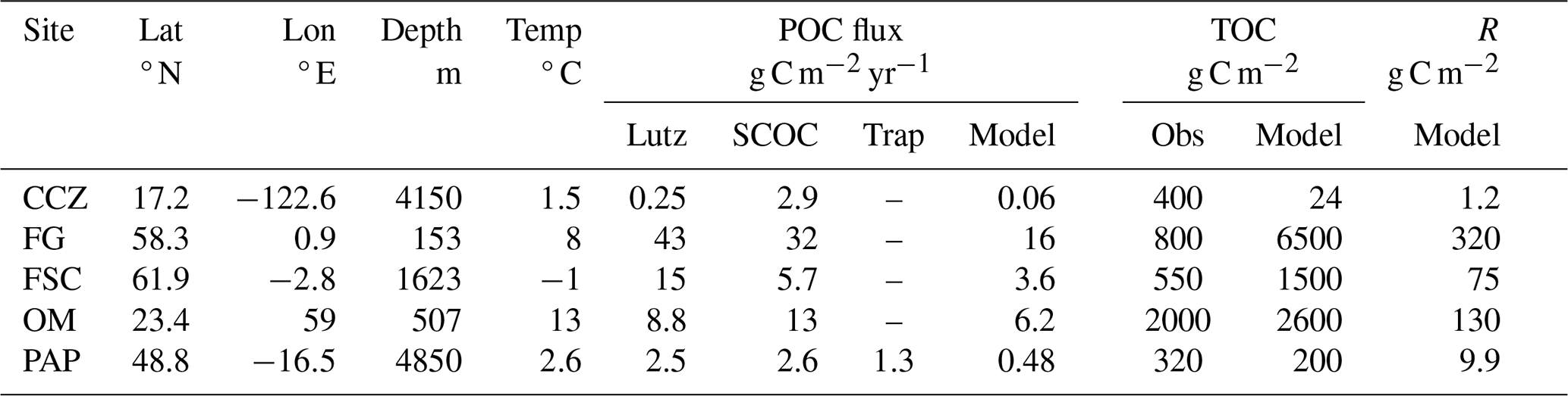
Table 2 Information on sites from which data were used to constrain parameter values for the general purpose parameter set given in Table 1, together with model diagnostics. POC flux is at the seafloor, estimated using the algorithm in Lutz et al. (2007), SCOC or sediment trap. TOC estimates come from Parameswaran et al. (2025). The “Model” columns indicate model diagnostic values. Model TOC is calculated by assuming that R is 5 % of TOC. Sources for data are given in Sect. 2.5.

The following first describes the observational constraints. Based on these, the argument for the specific choices of parameter values is then given. Table 1 has a summary of parameter values and Figs. 3 and 4, and Table 2, summarise the observational constraints and associated model diagnostics used to select them. The code needed to generate Figs. 3 and 4 is also available to allow the model to be re-tuned given additional data, different locations or different priorities (Martin et al., 2026).

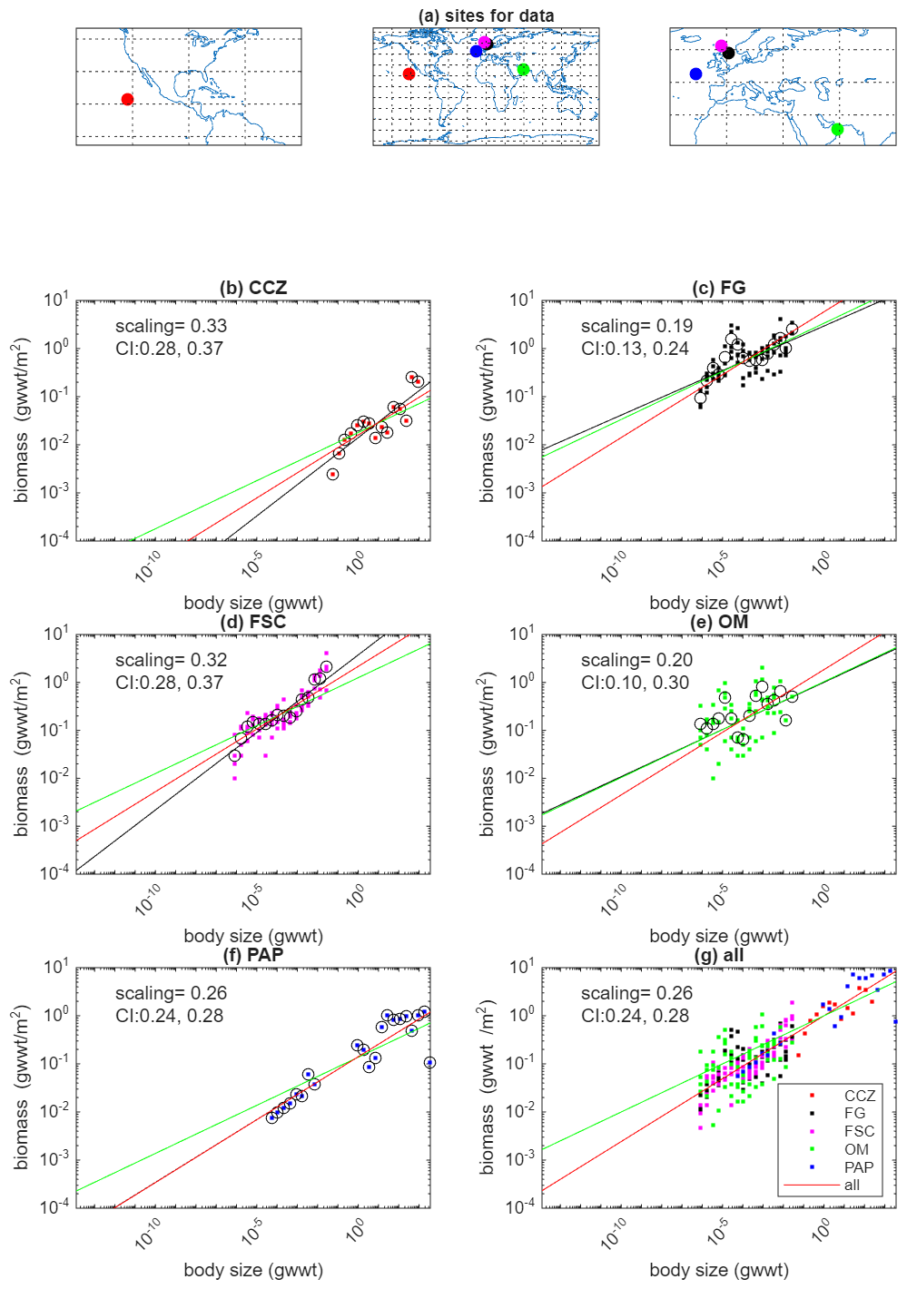
Figure 3 Locations (a) and observations of biomass as a function of body size for the five sites listed in Table 2. For each of the sites the dots show observations, circles indicate means within size classes and the black line is a power-law fit to the observations. The fitted values for the scaling exponent together with 95 % confidence intervals are also shown. The bottom right panel shows the fit to all sites simultaneously, assuming a common scaling exponent (fitted value shown with 95 % CI) but allowing the pre-factor to vary across sites. The dots show data from the sites with colours matching those used in the panels for individual sites. Note that in the bottom right panel the data from each site has been normalised by dividing by the fitted pre-factor to allow the visual comparison. The red line in all panels is the simultaneous fit to all sites. The green line in all plots is the relationship used in the model by fitting a power-law with an imposed scaling of 0.2 to the same observations.

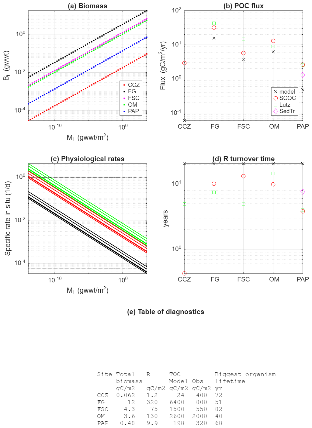
Figure 4 Model diagnostics and observational constraints: (a) modelled biomass (g wwt m²) size distributions for the five sites; (b) POC flux estimates using the Lutz et al. (2007) algorithm (Lutz), SCOC data (SCOC), sediment trap observations (SedTr) and the model constrained by biomass data from each site (model). Note that sediment trap data are only available for PAP; (c) model specific rates for maximum net growth (green), respiration (red) and mortality (black) for each of the sites. Note that they differ between sites because of the temperature effect. The two dotted black lines correspond to the constraints of a maximum growth rate of 1 d⁻¹ for the smallest organisms and a lifetime of 50 year for the largest organisms; (d) turnover time (R/POC flux) for each of the sites, estimated using model estimates of R and all observation and model estimates for the POC flux from (b); (e) a summary table of diagnostic parameters including total biomass (model), R (model), TOC (model and observations) and biggest organisms' lifetime (model).

Starting with the largest dataset, biomass can be used as a constraint for the interference parameter α. The steady state solution (Sect. 2.4) shows that a_i must scale in the opposite way to biomass distributions. Suitable observations from five sites are available in selecting the value; a summary is found in Table 2. The Clarion Clipperton Zone (CCZ) is a vast abyssal plain in the northeast Pacific. The data used here come from a site (17.2° N 122.6° W) of depth 4150 m with a low temperature (1.5 °C). Fladden Ground (FG) is in a shelf sea (153 m) and, unsurprisingly, with higher temperature (8 °C). The Faroe-Shetland Channel (FSC) is a connection between the North Atlantic and the Arctic, with the lowest temperature (−1 °C) despite a depth of only 1623 m. The Oman Margin (OM) is a slope site (507 m) and has the highest water temperature (13 °C). The final site is the Porcupine Abyssal Plain (PAP), which is the deepest (4850 m), with reasonably cold temperature (2.6 °C). A general decrease of temperature with depth is overlain with considerable variability due to local hydrography (notably FSC and OM). In addition to spanning a range of contrasting temperatures and depths, the data from the five sites also covers complementary size ranges of organisms. CCZ data are based on photographically surveyed megabenthos. FG, FSC, and OM data are based on physically sampled meio- to macrobenthos. PAP is based on physically sampled macrobenthos and photographically surveyed megabenthos. For CCZ, the data can be found in Benoist (2020), with sampling and methodology described in Simon-Lledó et al. (2019) and Benoist et al. (2019). Details on data for FG, FSC and OM can be found in Kelly-Gerreyn et al. (2014). Additional information on the sampling and laboratory methodology can be found in Kaariainen and Bett (2006). The benthic ecosystem of the PAP site has been studied for decades (Hartman et al., 2021). The data used here, and presented in Benoist (2020), combines analyses of macrobenthos and megabenthos. Descriptions of observational approach and the analysis methodology for the megabenthos can be found in Morris et al. (2016) and Durden et al. (2020b). For macrobenthos, this information can be found in Benoist (2020) and Ruhl et al. (2023). Further details on the treatment of size-resolved data, e.g. to remove biases such as under-sampled size groups, can be found in Edwards et al. (2017, 2020) and Ruhl et al. (2023). Observations of biomass versus size for each of the sites are shown in Fig. 3. These are referred to as biomass spectra and the gradient of the relationship (when plotted log–log as here) as the spectral slope, or scaling exponent. Despite some variability, all sites exhibit an increase of biomass with body size, and in a manner that is consistent with a power-law relationship. Figure 3 also shows the exponents found by fitting a power-law to the observations from each site individually. There is no strong relationship between fitted exponent and environmental parameters, though the smaller magnitude scaling exponents for the two shallow sites is something that has previously been seen in physiological rates rather than biomass (Mahaut et al., 1995). The OM site additionally has a low oxygen concentration (Demopoulos et al., 2003) which has been suggested to have a disproportionate impact on larger organisms (Quiroga et al., 2005) and which could therefore be responsible for flattening the slope relative to other sites. Nevertheless, here we take the simplest assumption that all sites are showing sufficiently similar behaviour in scaling to assume a common scaling exponent across the sites, leaving an investigation of departures from this for other studies. Figure 3g shows the simultaneous fit to data from all sites. It is seen that observations from the five sites cover different size ranges such that the composite dataset spans a substantially wider size range than any individual site. Furthermore, the relationship of biomass with size appears consistent across the wider range. If the data from all sites is combined then the scaling exponent for a power-law fit to all five sites simultaneously indicates a scaling exponent of 0.26 (s.d. 0.016, r²=0.76, p<0.001). The existence of similar scaling behaviour across multiple sites gives more confidence that the model can be used globally.

The next observational constraint comes from the requirement that the supply of organic carbon to the ecosystem (the POC flux, F) balances the total respiration of the organisms present at steady state. For the model, respiration is given by the sum over size classes of the product of the specific respiration rate and biomass in each size class, Σr_iB_i. Therefore, observations of POC flux, co-located with the previously described size-resolved estimates of biomass, provide a useful joint constraint on r₀ and β. There are several sources of data for POC flux. First, and most directly, for the PAP site there is a long time-series of sediment trap data (Lampitt and Pebody, 2023). Although there are sediment traps at both 3000 and 4750 m, the latter is thought to be biased by sediment resuspension as it is just 100m above the seafloor. The magnitude of this effect can vary with time but previous work has shown that the flux near seabed at the PAP site is often in excess of that at 3000 m due to re-suspension (Lampitt et al., 2000, 2001). For this reason, it is better to extrapolate the estimate from the 3000 m trap. For the year 2012 (to best match the biomass observations) the annual carbon flux at 3000 m is 1.91 g C m⁻² yr⁻¹. The associated flux at the seafloor can be roughly estimated using a widely used power-law scaling (Martin et al., 1987), such that the flux at the seafloor at 4850 m equals 1.91  C m⁻² yr ⁻¹ ⋅ (3000 m/4850 m)^0.858 = 1.3 g C m⁻² yr⁻¹. An alternative way to estimate the sinking flux at the seafloor is to use the Lutz et al. (2007) algorithm, which uses net primary production, sea surface temperature and depth at a given location to estimate the flux. This allows estimates to be made for all five sites (not just PAP) – see Table 2. Finally, Sediment Community Oxygen Consumption (SCOC) data (Stratmann et al., 2019) also allows the sinking flux to be estimated, making the same assumption that the respiration (measured by oxygen consumption) must balance this flux, in this case when averaged over the year. As SCOC is usually measured using chambers of ∼50 cm across, the estimates exclude or bias the contribution from larger organisms – not just those too large to fit but also those too scarce to be robustly sampled in such an area – and care is needed in accounting for this (Laguionie Marchais et al., 2020). More generally, all of these sources of POC flux data have significant associated uncertainties, which is why POC flux was not fixed when deriving parameter values for the general use model configuration described here. Instead the model can be used to estimate the POC flux and compared to these different observational estimates as a broader constraint. All observational estimates of POC flux used to constrain model parameters, as well as the model values, are shown in Fig. 4b. These values are also given in Table 2. Note that even if there was no uncertainty in the observations for POC flux it would still not be possible to infer specific values for β and r₀ using the data. This is because it is possible to simultaneously vary β and r₀ in a way that the total respiration remains unchanged. Note that respiration also gives a link between the physiological (β) and interference (α) scaling exponents that needs to be considered. Respiration by a size range of organisms is given by r_i⋅B_i, which scales as $M_i^{\mathit{\alpha }-\mathit{\beta }}$. Hence, the difference between α and β determines whether the energy use by a size range increases (α>β), decreases (α<β) or remains the same (α=β) with size. We are unaware of observations indicating an increase with size but there are observations suggesting α=β (Laguionie Marchais et al., 2020) and this is consistent with “energy equivalence” which has been suggested theoretically (Damuth, 2007).

The inherent relationships between the three physiological rates allow other observational constraints. Observations indicating that physiological rates decrease with size were already described. Additionally, the maximum net growth rate, g_i, must equal or exceed the sum of the respiration, r_i, and mortality, m_i, for all sizes for populations to be sustainable. Together, these two statements imply that all rates must sit within a “window” of parameter space (rate versus size, Fig. 4c). We follow a similar approach to that of Mahaut et al. (1995) and Kelly-Gerreyn et al. (2014), by using constraints at smallest and largest sizes of organism. Having so many degrees of magnitude in size in the model means that care is needed for the parameter values to be realistic at the two extremes of the sizes reproduced. Using constraints at intermediate sizes risks significant under- or over-estimates for largest and smallest organisms through under-constrained extrapolation. Because rates are observed to decrease with size, the top left corner of the window is set by the upper limit for the specific growth rate of the smallest size class of organism. For benthic bacteria, we take a rough upper limit of 1 per day maximum specific growth rate. Though Dixon and Turley (2001) find a rate of 0.1 per day, a wide range reported by Giovannelli et al. (2013) includes a value of 6 per day. An intermediate value of 1 per day is marked in Fig. 4c. The bottom right corner of the window is set by the lower limit for the specific mortality or respiration rate (whichever is smallest) of the largest size class. The data collated by McClain et al. (2012) indicates lifetimes for the largest organisms (few kg wwt) of order 50 years. Given this and assuming the same scaling, β, for all physiological rates as stated earlier, comparison to POC fluxes described above indicates that respiration is a considerably larger rate than mortality, so mortality defines the bottom right corner of the “window”. This is also marked in Fig. 4c and lifetimes for the largest organisms at each site are also given in Fig. 4e. Note that both of these constraints need to be treated a little flexibly as it is not realistic to set a precise limit in either case.

There are two further constraints, to inform the choice of values for β, g₀, r₀, m₀ and E. First, the ratio $(r_{\mathrm{0}}+m_o)/g_{\mathrm{0}}$ represents the fraction of the maximum growth rate, g₀, achieved by organisms when the system is in equilibrium. This should take a value less than 1 for food to be limiting, as is expected for the seafloor (Smith et al., 2008). Second, decreasing E converges physiological rates for the different sites, as the inter-site differences due to temperature are diminished. Doing so reduces the inter-site differences in model POC flux (and R) for the same reason, because of the balance with total respiration.

The final observational constraint is Total Organic Carbon (TOC) in the benthic sediment which can be used to estimate the amount of detritus available as food, R, which itself is a constraint on the parameter a₀. This can be seen in the steady state solution (Eq. 13), where R increases linearly with a₀. We make use of the compilation of Parameswaran et al. (2025) who created an atlas of TOC at the seafloor surface, using a neural network approach applied to globally distributed estimates calculated over the top 10 cm of sediment. This data source was chosen in preference to the alternative product of Atwood et al. (2020) as the latter used estimates over the top 1m of sediment, which are an order of magnitude larger than those in Parameswaran et al. (2025) and likely to represent carbon resources unavailable to the majority of detritivores on the seafloor. The estimates for TOC using Parameswaran et al. (2025) for the five sites are shown in Fig. 4e. These are not directly comparable with R, however. There is considerable evidence that not all of sediment TOC is readily available as a food resource, with typically 5 % (e.g. de Jonge et al., 2020; van Oevelen et al., 2011a, b) regarded as “labile” i.e. easily consumed (see Discussion for more on this). We therefore multiply our model estimates for R at the five sites by a factor of 20 to give an estimate of TOC for comparison to the observational values. Estimates for TOC based on Parameswaran et al. (2025) are given in Fig. 4e and Table 2, together with model estimates for R and TOC. There is considerable variability; in observations, model values and their relative sizes. A weaker constraint for a₀ is the turnover time for R i.e. the time it would take for R to be replaced by the POC flux (Fig. 4d). A minimum turnover time of several years would be expected for the system to be able to achieve steady state on an annual basis.

We now outline our choices of parameter values (Table 1) given the above constraints. Starting with α and β, taking $\mathit{\alpha }=\mathit{\beta }=-\mathrm{0.2}$ gives a scaling exponent consistent with observations for rates and energy equivalence but requires a biomass scaling that is a little lower than the fit to observations. It is not possible to use the −0.26 scaling implied by the observed biomass spectra without substantially worsening the fit between model and observational estimates of POC flux (Fig. 4b). Given this scaling for β, we take g₀=0.001, r₀=0.0045, m₀=0.0005 per day to fit rates within the window in Fig. 4c. This also gives a value for $(r_{\mathrm{0}}+m_{\mathrm{0}})/g_{\mathrm{0}}$ of 0.5, giving food limitation at steady state. We take a value of E=0.35 eV which is at the low end of observations but using a larger value also worsens the match between model and observational estimates of POC flux. Finally, a value of 2000 is taken for a₀ as it gives the best agreement between model-estimated and observed TOC (Table 2) across the sites given the other choices of parameter values.

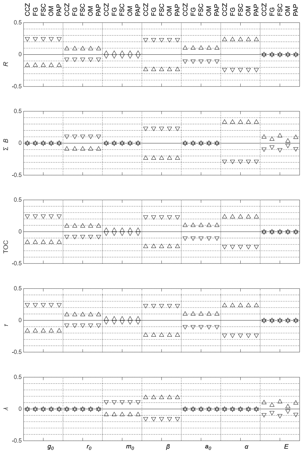
Figure 5 Sensitivity of the metrics detritus (R), total biomas (ΣB), TOC, turnover time of detritus (T) and lifetime of largest organism (λ) to each of the model parameters across the five sites. In each case the sensitivity shows the fractional change resulting from a ±10 % change in the parameter from the standard value. Symbols point in the direction in which the parameter was changed i.e. upward-pointing pyramids indicate an increase in parameter value and inverted pyramids indicate a decrease.

The sensitivity of key metrics to the model parameters is shown in Fig. 5. For each metric, its fractional change for a ±10 % change in parameter value, from the values given above, is shown. This was carried out for each site assuming the observed temperature and the POC flux that is consistent with a model fit to the biomass observations at that site with the imposed 0.2 scaling exponent. The three parameters g₀, α and β show the greatest sensitivity, with a 20 %–30 % change for a 10 % change in parameter. The exceptions are: the largest organism lifetime, which is insensitive to g₀ and α; and total biomass, which is insensitive to g₀. It should be noted that the sensitivities of α and β work in opposite directions, with a decreased metric for one corresponding to an increase in the same metric for the other. This means that any simultaneous change to these parameters while retaining energy equivalence (i.e. α=β) would have a reinforcing rather than a compensating effect. Although only the parameter g₀ shows a clear asymmetry about zero for the sensitivity analysis in Fig. 5 it should be noted that the metrics are generally non-linearly dependent on the parameters. This becomes more apparent if a larger fractional change to parameters in the sensitivity analysis is used. There are some cases where a metric is linearly dependent on a parameter though (e.g. R on a₀ – see Eq. 13) and in these cases the effect of a ± parameter change will always be symmetrical about zero. An obvious feature of the sensitivity analyses is that only E has an influence which varies across sites. This is the combined effect of two factors: temperature and POC flux are the only external influences that vary between sites; and the sensitivity analysis shows fractional, not absolute, changes in the metrics i.e. the sensitivity is calculated as the metric evaluated at the altered parameter value divided by that obtained using the standard value. Using the steady state solution (Eqs. 10 and 11) and taking each metric in turn we can see how this cross-site consistency arises. For R, as it varies linearly with the POC flux, the flux cancels out in the sensitivity calculation. The temperature effect (Eq. 4) varies across sites, but R is already insensitive to this because growth, respiration, mortality and interference all share the same temperature dependence and their effects cancel each other out (Eq. 10). As TOC is calculated simply as a constant multiple of R, it shares the lack of variation in sensitivity across sites. Similarly, the turnover time (τ) is calculated as the ratio of R to the POC flux, the latter of which cancels when calculating the metric (as described above). Thus, τ also shows a sensitivity that is constant across sites. The two metrics of total biomass (ΣB) and lifetime of largest organism (λ) do vary across sites for one of the parameters, the activation energy E. The steady state solution for biomass (Eq. 11, but perhaps clearer in Eq. 12) shows that it varies with temperature due to temperature's influence (via θ(T)) on physiological rates (specifically the respiration rate) for which E is the key parameter. The sensitivity of total biomass to E is dictated by the ratio of θ(T) calculated at altered and original values. Because θ(T) is a non-linear function of T and E, this ratio varies across sites. Similarly, as the lifetime of the largest organisms is simply the reciprocal of their mortality, a physiological rate which varies with θ(T) across sites, then it will too. For the other parameters, neither temperature nor POC flux give rise to variation in sensitivity across sites: none of g₀, r₀, m₀, a₀, α, or β exert an influence through changes in temperature; biomass varies linearly with POC flux (Eq. 11), which therefore cancels out when calculating the sensitivity; and the lifetime of the largest organisms has no dependency on the POC flux.

2.6 Model performance

The observations at all five sites show a power-law distribution of biomass with size, and the model performs well in capturing this characteristic at each site (Fig. 3). Note that the matching of magnitudes in biomass for each size class across sites in Fig. 3g arises from the normalisation for the simultaneous fit, not directly from model parameter value choices. Although the choice of E influences the differences in biomass across sites, they are also influenced by inter-site differences in POC flux. For POC flux (Fig. 4b and Table 2), although there is some variability within the observations, the model and observational estimates agree reasonably well and vary in a similar way across the sites. All have lowest fluxes at the deepest sites (CCZ, PAP), highest at the shallowest (FG), and the fluxes at these two extremes differ by 1–2 orders of magnitude. For the physiological rates, in Fig. 4c the lines showing the rates should fall within “window” marked as dotted black lines, and described in Sect. 2.5. It is seen that although this is broadly the case, the chosen parameter values already lead to this “window” being stretched. Maximum bacterial (smallest size class) net growth rate is between 2–4 per day across the sites, higher than the reference value of 1 per day. The net growth rate achieved at equilibrium to first order matches the respiration rate because mortality is so much smaller, and varies between 1–2 per day. Life expectancies for the largest organisms are seen to span 40–82 year and straddle the reference value of 50 year. Estimates for TOC using the model vary from 24 to 6400 g C m⁻². The observed range is smaller (from 320 to 2000 g C m⁻²) but given the large variability in observation and model estimates across sites, the match is reasonable; at some places the model exceeds the observed value and at others it is lower. The turnover time (Fig. 4d) is seen to be estimated at ∼20 year, using the model estimated POC flux. It is lower (3–15 year) using the observations for POC flux (Fig. 4b) and model estimate of R because the model under-estimates the POC flux. Overall, using this set of parameters, the model does a reasonable job of satisfying the constraints while simulating the biomass size distribution of the ecosystem at strongly contrasting locations.

2.7 Uncertainty in parameter values

Like any other ecosystem model, there is no single objective choice of parameter values. The sensitivity analysis shown in Fig. 5 and discussed in Sect. 2.5 indicates the consequences of changing the current values. Additionally, it is insightful to understand some of the restrictions on changing the values of the parameters.

A significant constraint arises from the mass scaling exponent for the biomass observations at the different sites. If the scaling exponent is estimated using data from just a single site (Fig. 3a–e), the estimates vary from 0.19 (for FG) to 0.33 (for CCZ). The uncertainty is largest at OM (CI: [0.1, 0.3]) and smallest at PAP (CI: [0.24, 0.28]). If data from all sites are combined, as described in Sect. 2.5, then the exponent is estimated at 0.26. A sensitivity analysis was done on how the estimate varies if data from each site in turn is excluded. Excluding data from CCZ, FG, FSC, OM and PAP in turn gives a value that varies between 0.25 and 0.27. Hence, none of the individual sites is having a significant effect on the estimate of the biomass scaling exponent. As described in Sect. 2.5, the value used for the interference scaling exponent in the model is equivalent to having a biomass scaling exponent of 0.2, below the values obtained from the observations described above. Also as described in Sect. 2.5, using a greater magnitude value would either lead to a dominance of respiration by larger organisms (rather than the “energy equivalence” for which there is some observational support) or require an equivalent increase in the magnitude of the scaling exponent for the physiological rates.

The chosen value of −0.2 for the exponent, β, is within the range of observational estimates. Most of these cluster around −0.2 to −0.25 (e.g. Mahaut et al., 1995  Ernest et al., 2003). Lower values have been found though. McCoy and Gillooly (2009) reported an exponent of −0.18 for invertebrates. Lower still, McClain et al. (2012) found an exponent of −0.11 for growth of benthic organisms, though noted that this was inconsistent with the exponents they found for respiration and mortality (−0.2 and −0.24 respectively). Looking at Fig. 4c it is apparent that a using larger magnitude (perhaps to allow a biomass scaling of 0.25 and retain energy equivalence) would lead to a lower average respiration rate across the size classes, as the respiration rate for the smallest size organism cannot get any bigger. An increase in the magnitude of β would, therefore, lead to a reduction in the model estimate of the POC flux and the quality of its fit to observations. For example, if β were changed to −0.25, then r₀ would need to be reduced by a factor of 5 to meet the constraint arising from the maximum bacterial growth rate and the model POC flux estimates would therefore also decrease by a factor of 5, making them a further factor of 5 lower than observations, which the model already underestimates.

The value chosen for E (0.35 eV) is at the lower end of values derived from observations. For a range of organisms not restricted to marine ones, Savage et al. (2004) found values from 0.35 to 0.84 eV. McClain et al. (2012) estimated E as 0.47 eV for respiration and mortality but, with less confidence, 0.16 eV for growth. McCoy and Gillooly (2009) found a value of 0.69 eV for respiration. For comparison, the canonical value for MTE is 0.63 eV (West et al., 1997; Brown et al. 2004). The greatest influence of E is in accounting for significant differences in physiological rates between sites with strongly contrasting temperatures. Changing temperature from 0 to 10 °C with E=0.35 eV increases rates by a factor of 1.7. Using E=0.63 eV increases rates by a factor of 2.6. However, if E=0.63 eV then model-estimated POC fluxes reduce by 24 %–57 % across the sites. This is because the temperature effect θ(T) takes lower values with the larger E even though the difference between θ(T) at different temperatures is greater.

The greatest subjectivity in choice of parameter value is in deciding the ratio $(r_{\mathrm{0}}+m_{\mathrm{0}})/g_{\mathrm{0}}$ which represents the fraction of the maximum growth rate that an organism achieves at equilibrium. Another perspective on this is that it represents the degree of food-limitation, with a value of 0 representative of total starvation and a value of 1 of a surfeit. We subjectively took this ratio to be 0.5 to be consistent with a food-limited ecosystem which is dependent on material that is already the meagre remains of food that was available to many other organisms as it sank down through the water column (Smith et al., 2008). It should also be appreciated that two locations with high and low food supplies do not necessarily differ in the degree of food limitation, as the population sizes at the two sites will reflect the supplies. It is unlikely that direct observations will become available to constrain this ratio so changes to the current value are more likely to arise from a wish to change one of the three component parameters, g₀, r₀ or m₀. Keeping β fixed, the first two of these, g₀ and r₀, are already at the upper limit of observations whilst m₀ is at the lower limit (Fig. 4c). Figure 5 shows that decreasing g₀ by 10 % would lead to a ∼25 % increase in R, TOC and turnover time. It would also increase the time for the perturbed system shown in Fig. 7 to recover to 95 % of the steady state value from 59 to 71 years. A 10 % decrease in r₀ would result in the same decrease in estimated POC flux (or a compensating 10 % increase in total biomass if it was wanted to preserve the total respiration, Fig. 5). The same 10 % decrease in r₀ would give a ∼10 % decrease in R, TOC and turnover time (Fig. 5). Finally a 10 % increase in m₀ would give a 10 % decrease in lifetime for the largest organism. Returning to the ratio $(r_{\mathrm{0}}+m_{\mathrm{0}})/g_{\mathrm{0}}$, a 10 % decrease in r₀ and m₀ would give a 10 % decrease in the ratio to 0.45. Decreasing g₀ by 10 % would increase it by 11 % to 0.56.

A change in a₀ results in a corresponding change in R (Eq. 13 shows that they are proportional at steady state) and consequently for the model estimate for TOC. The current value of a₀ was chosen to minimise ${\mathrm{\Sigma }}_{\mathrm{sites}}\left[\log \right({\mathrm{TOC}}_{\mathrm{est}}/{\mathrm{TOC}}_{\mathrm{obs}}){]}^{\mathrm{2}}$. Obviously, the choice of a₀ is sensitive to the subjective choice of this function. If a simple sum of squared differences was used instead then a choice of a₀=500 would be more optimal, giving a lower range of estimates than those given in Fig. 4e and Table 2 (9.2 g C m⁻² CCZ; 2400 g C m⁻² FG; 560 g C m⁻² FSC; 960 g C m⁻² OM; 74 g C m⁻² PAP). We used the logged ratio to choose a₀ here because of the orders of magnitude difference between observations across the sites (Fig. 4e, Table 2). Using a simple sum of squared differences biases the value to best fit observations with largest TOC concentrations. The turnover time of R i.e. the time it takes the POC flux to replenish R if removed, has the same sensitivity to a₀. This can affect the recovery time to perturbations. Having slower recovery of R increases the recovery time for small organisms that would otherwise recover much quicker than large ones because of higher physiological rates. The small organisms cannot fully recover until R itself is recovered. This is apparent in the example of how BORIS2 may be used to study a response to a change in POC flux given later (Sect. 3.2 and Fig. 7). Using a value of 500 in this example would reduce the time taken for the total biomass to recover to 95 % of the steady state value from 59 to 27 years. Turnover times estimated using the model are also affected by choice of a₀ as shown in Fig. 5d. They are consistently ∼20 years for the current choice of a₀ but reduce to 5 years if a₀=500.

3 Use of BORIS-2

BORIS-2 runs easily and quickly in Matlab (it was developed, tested and run in version 25.1.0.2973910 (R2025a) Update 1, and a steady state solution (Sect. 2.4) is available for situations where equilibrium is the focus. The model requires only the seafloor temperature and POC flux for a location as inputs. If BORIS-2 is to be used at a specific location then it may be possible to estimate the local POC flux directly using in situ data from sediment traps (e.g. Durden et al., 2020a; Smith et al., 2013), although the resuspension of material means that near seafloor data should be treated with care. Alternatively, if it is intended to use BORIS-2 over larger areas, such as basin scales, then POC flux can be estimated less directly using algorithms which estimate POC flux at any given depth using satellite remote sensing data (Lutz et al., 2007) or using global biogeochemical model output (e.g. Yool et al., 2017; Fig. 3.21 of Cooley et al., 2022). Alternatively, observations of sediment community oxygen consumption (SCOC) rates (Smith et al., 2013; Stratmann et al., 2019), which would be expected to roughly balance POC input on timescales for which the system could be viewed as in steady state, could be used. We now give a few examples to illustrate the range of potential uses.

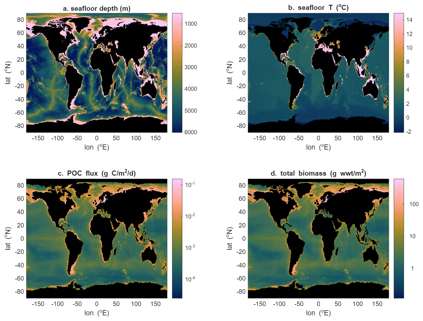
Figure 6 Example of using the steady state solution (Eqs. 10 and 11) to explore spatial variability in total benthic biomass: seafloor depth (a) and temperature (b) from the World Ocean Atlas, particulate organic carbon (POC) flux (estimated using Lutz et al., 2007) (c), and total biomass (d).

3.1 Using the steady state solution

If it is of interest to know how benthic biomass (i.e. the total amount of organisms that can be sustained) varies geographically, it is useful to focus on the annual average biomass such that it can be assumed that the ecosystem is in steady state to first order. This assumption allows Eqs. (10) and (11) to be used for quicker calculations. In Fig. 6, use is made of data for POC flux and temperature at the seafloor to produce a global map of benthic biomass. The POC flux data are generated using the Lutz et al. (2007) algorithm while seafloor temperature data come from the World Ocean Atlas (Reagan et al., 2024). Temperature is largely uniform, with little change across the abyssal plains, or even above seafloor ridges, due to the weak vertical gradients in temperature in the deep ocean. The pattern of low values in subtropics with higher values in tropical, subpolar, polar and coastal regions for the POC flux is similar to that seen in the export of organic material from the ocean surface (e.g. Nowicki et al., 2022) but superimposed on this is the effect of depth. POC flux attenuates strongly with depth (Martin et al., 1987), and a logarithmic scale is needed to capture the variation in seafloor POC flux from shelf to abyssal regions. Because of the largely uniform distribution of seafloor temperature, that of seafloor biomass closely resembles that of the POC flux for much of the ocean. Only in the Mediterranean and Red Sea are the impacts of much higher temperatures visible with lower biomasses relative to the variations in POC fluxes because they need to balance greater physiological rates.

3.2 Running the model dynamically

The dynamic version of BORIS-2 runs easily on a standard laptop, taking just seconds for a thousand years. The forcing data on POC flux, F, and the temperature, T, can also both vary with time if required. This allows a variety of transient responses to be explored.

For temperature, long-term temporal change in deep-water temperatures has been detected, but is of a very small magnitude (e.g., <0.002 °C yr⁻¹, Garry et al., 2019). Stronger fluctuations at a site may arise near the boundaries of warm (e.g. Red Sea, Mediterranean Sea), cool (e.g. Atlantic, Pacific, Indian Oceans), or cold (e.g. Arctic and Southern Oceans) deep waters if their boundaries move in response to natural or climate-change related shifts. For example, at the Arctic-Atlantic transition in the Greenland-Iceland-Faroe-Shetland region a 10 °C shift in bottom water temperature can occur over a short spatial (bathymetric) scale (e.g., Turrell et al., 1999) and so a near 10 °C shift can occur on short time scales (hours, e.g., Bett, 2001). Generally, though, because a 10 °C change in temperature is required to create a roughly factor of 2 change in physiological rates, scenarios where time-varying temperature has a significant impact on biomass are likely to be rare for deeper, off-shelf locations.

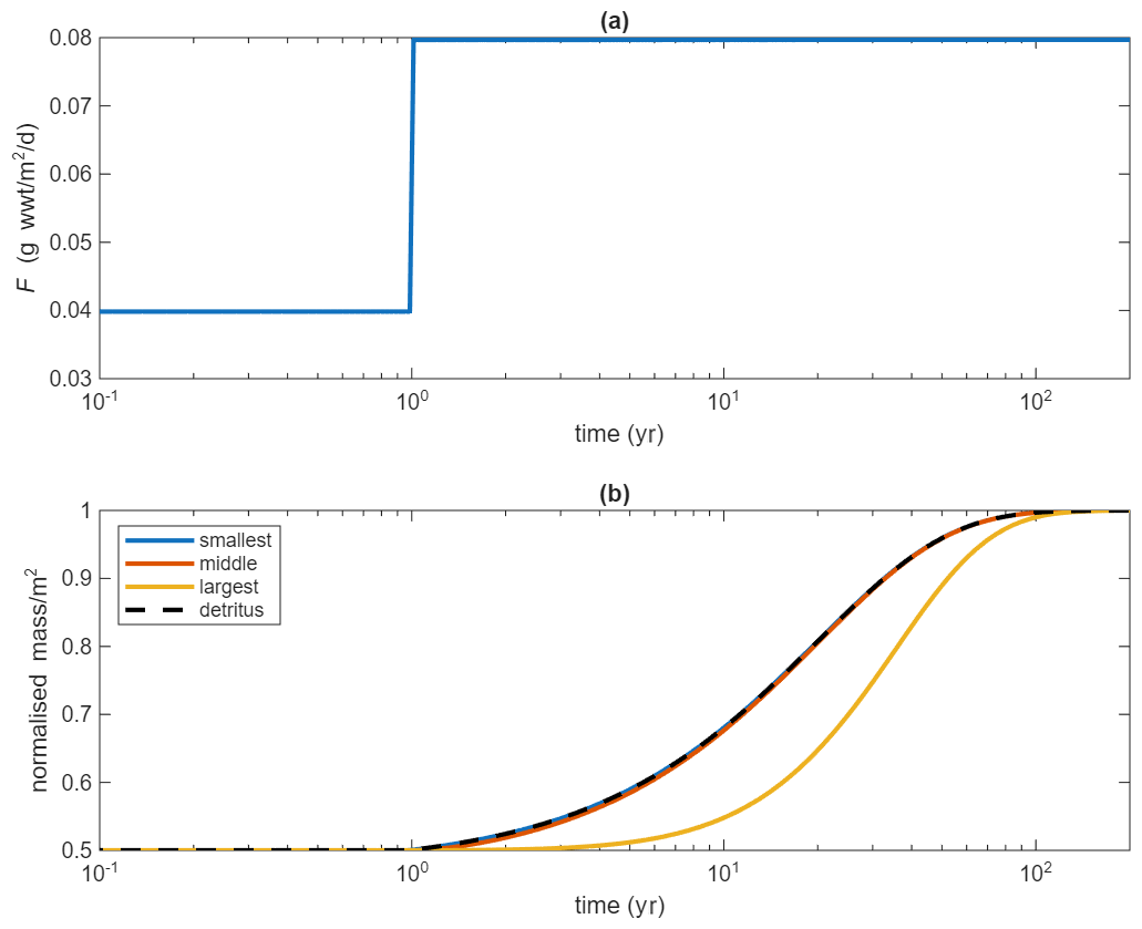
Figure 7 Modelled response to a perturbation in which the ecosystem is initially in steady state and then a doubling of the POC flux takes place: (a) shows the POC flux, with doubling occurring after 1 year; (b) shows the response of organisms and detritus. For clarity only 3 size classes are shown, the smallest, middle and largest (i=1, 30 and 59). For the same reason, the biomasses and detritus are normalised by dividing by their final value. A log time scale is also used to highlight the different response timescales.

Significant changes in POC flux are more likely. For example, considerable uncertainty remains over the impact of climate change on export of organic carbon from the ocean surface but future changes of up to 41 % are possible (Henson et al., 2022). Such changes in POC flux leaving the surface will impact the benthic ecosystem, which is dependent on the fraction of this export that reaches the seafloor. One application of the dynamic version of BORIS-2 therefore is in exploring climate change consequences for the benthos (e.g. Yool et al., 2017). A much simpler example of how the model can be used to study responses to change in POC flux is shown in Fig. 7. Here the ecosystem is initially in steady state but then the POC flux is doubled. As is apparent in Figure 3, the different sizes of organisms will have very different biomasses. Hence, for ease of comparison the biomasses and detritus are normalised in Fig. 7 by dividing by their final value. Similarly, the variation of physiological rates with size means that response times differ with size of organism. Using a log time scale allows this to be seen more clearly. The smallest size class tracks the response of the detritus closely because faster physiological rates allow these organisms to respond as quickly as the detritus changes. The larger organisms have slower rates and are seen to respond significantly more slowly as a consequence.

4 Discussion

The BORIS-2 model has been presented. It allows simulations of the benthic community across the full size-range of organisms. A single parameter set has been provided for general use that allows the model to reproduce observed biomass size distributions at five sites contrasting strongly in location, depth and temperature, while meeting other constraints on POC flux, expected physiological limitations of smallest and largest organisms and the amount of organic carbon available for food on the seafloor. It is intended that BORIS-2 be used in a macroecological manner, not to represent the dynamics of specific species. Physiological processes for organisms within the same size class can vary significantly so BORIS-2 is best suited for examining questions related to the overall community or the relative behaviour between size classes. As with any model there are aspects that represent limitations and, as a result, areas for further investigation.

4.1 Model assumptions

BORIS-2 assumes all organisms are detritovores feeding from the same common resource, detrital organic carbon on the seafloor. In practice, a community will have organisms exhibiting a variety of feeding strategies of which detritivory is just one. Predation, for example, is not captured explicitly by BORIS-2. However, on seafloors deeper than the euphotic zone and outside of chemosynthetic systems, the benthic ecosystem is supported solely by the POC flux and predation is effectively a secondary transformation of that carbon. One interpretation is that BORIS implicitly captures predation in the mortality term but that the gains are distributed across all size ranges rather than received by specific ones. Even from that perspective, BORIS-2 may under-estimate predation because mortality is parameterised based on natural mortality rate data. In the absence of suitable data for predation rates and given the large uncertainties in natural mortality, the magnitude and significance of this underestimate are uncertain. Separate population dynamics for detritivore and predator components of the benthic community have been studied on the shelf (Blanchard et al., 2009) where it was found that predators might display a stronger increase of biomass with size than detritivores. A size-based model presented in the same work to explore this interaction further found that the presence of predators could cause a steepening of the biomass spectrum for detritivores where their size overlapped with the prey range for predators. However, the predators of benthic organisms were assumed to be largely pelagic – a condition that is not experienced in the deep ocean. While a similar coupled approach could be adopted in BORIS-2, the main difficulty in incorporating carnivory into BORIS-2 is the requirement for data on the relative abundance of predators versus non-predators across size classes. Such data are scarce even on the shelf (e.g. Blanchard et al., 2009). Without such information it would be difficult to constrain sufficiently the model parameters.

An additional facet of the ecosystem that is simplified by BORIS-2 is how the organisms obtain their food. In reality, they may be more or less mobile, allowing them to search for food. They may also be able to filter organic matter from seawater as suspension feeders, intercepting food before it hits the seafloor or exploiting resuspended or advected material. In theory, the parameter a₀ could be modified to reflect greater mobility while the growth parameter, g₀, could be adjusted to capture the effect of suspension feeding. Once again though, to incorporate such changes would require additional data on the relative abundance of organisms with these different characteristics across size ranges.

A final assumption of BORIS-2 worth discussing is that no organic material is either refractory or buried. For burial, a fraction of the POC flux and/or the mortality could alternatively be regarded as buried and removed from the system. Note that the POC flux would then have to balance the sum of burial and respiration, so a lower respiration would be required to balance the same POC flux. Estimates for burial vary from 37 % of the POC flux arriving at the seafloor on the shelf to 4 % in the deep (>2000 m) ocean (Dunne et al., 2007). The shelf value is in the absence of perturbations to the sediment such as fishing related trawling. Based on the low deep-sea fraction, burial is omitted. It could easily be added as a (depth-dependent) “tax” on seafloor POC flux if needed subsequently. Regarding refractory organic carbon, it was described in Sect. 2.5 that it has been assumed that only 5 % of the total organic carbon in the surface sediment is readily available to the benthic ecosystem represented by the model. The other 95 % is regarded as refractory. Consider two scenarios. The first is that the POC flux arriving at the seafloor is entirely labile and refractory carbon is created only by the seafloor ecosystem. In this case, it would be possible to modify BORIS-2 such that a fraction of mortality passed into a refractory carbon pool rather than into R. In the second scenario, the POC flux has a refractory component. This could be directed straight into a refractory pool. Reality is likely to be some combination of these two scenarios. At steady state, all of the organic carbon entering the refractory pool must either be respired or transformed to labile material and hence returned to R. In the hypothetical case of no respiration, then the flux of organic material into and out of the refractory pool should balance, such that the net flux is zero. This is the implicit assumption in BORIS2, such that this exchange is not modelled. In reality, some of the refractory carbon will be respired, and this could be incorporated in BORIS-2 in the same way as burial, as a simple extra loss; applied to the POC flux or by adding creation and respiration of refractory material by the benthic community as appropriate. In the absence of data from multiple sites for the amount of refractory carbon arriving as POC flux or created by the benthic ecosystem, and the fraction of this that is eventually respired or buried, the dynamics of the refractory pool are omitted. An additional aspect of the refractory carbon dynamics is that there will be a bacterial population carrying out its respiration that is also not captured by BORIS-2. This means that observational estimates of bacterial abundance in seafloor sediments are likely to be higher than those predicted by BORIS-2. With a large pool of refractory carbon (Sect. 2.5) and associated bacterial doubling time up to thousands of years (Jørgensen and Marshall, 2016), this additional population is likely to be much larger than represented by the smaller size classes of the model that are feeding on R. For example, bringing together observations from a site in the abyssal Pacific to apply a linear inverse model for the benthic system including refractory carbon, de Jonge et al. (2020) estimated the prokaryotic biomass to be roughly equivalent to that for megafauna. In BORIS-2, the biomasses for the equivalent (smallest and largest) size classes differ by a factor of 10⁵. This is not a straightforward comparison though as the prokaryotes in the de Jonge et al. (2020) study feed from both labile and refractory material. If future data suggest that bacteria need to be taken out of the allometric framework and treated separately, the biomass estimates of remaining organisms are unlikely to change by more than a factor of two (the extreme case of bacteria having total biomass equal to all other organisms present), with relative biomass of other classes unchanged. To make such a change though would require information on the flux or fraction of organic carbon entering the refractory pool, and the physiological rates of the bacteria ingesting and respiring it. Note that the very definition of “refractory” is itself an uncertainty. The wide flexibility in the structure of molecules of organic carbon means that POC varies widely in how “labile” or “refractory” it is. It is not a simple binary, so this adds a further layer of uncertainty.

Nevertheless, treating bacteria differently could offer one means of increasing the total respiration to give an improved match to the observations for POC flux and oxygen consumption (Fig. 4b). As an extreme example, if only bacteria were allowed access to the POC flux arriving at the seafloor (rather than everything having equal access at present), with the detrital pool being supplied instead by dying bacteria, then the observed biomass of other organisms would be supported by a fraction of the POC flux equivalent to the ratio of mortality to respiration of the bacteria. This ratio is 0.1 for the current parameter set. Without changing any parameter values this approach would therefore decrease the POC flux available for other organisms in Fig. 4b by an order of magnitude, with respiration of those organisms now exceeding estimates, as anticipated. It would also increase bacterial biomass by two orders of magnitude (but still three orders of magnitude less than the total). Although there is some evidence that bacteria respond quickly to POC deposition (Sweetman et al., 2019), other similar studies show a wider response, including a rapid response by macrofaunal invertebrates (Witte et al., 2003). Note that the latter studies were conducted at small physical scales that effectively exclude megafaunal invertebrates such that their relative influences and responses are unknowns (Laguionie Marchais et al., 2020). The option to treat bacteria differently is therefore left for future study.

4.2 Other possible model extensions

An aspect of BORIS-2 which may benefit future development is the restricted number of external influences. There are currently only two: the supply of detrital material to the seafloor (POC flux) is the food source for all organisms and ambient temperature is the only control other than size on metabolic rates.

The effect of oxygen concentration in seawater is not currently included in BORIS-2. Although it has been questioned whether there is clear evidence for an oxygen effect on metabolism (Seibel and Drazen, 2007), a lack of clear response to low oxygen by benthic communities might be as a result of a shift in community composition towards organisms more efficient at extracting oxygen from waters with low concentrations (Childress and Seibel, 1998). That said, under reduced oxygen concentrations there is evidence that macrobenthos shift to smaller body sizes (Pearson and Rosenberg, 1978), while meiobenthos may shift to large body sizes (Moore and Bett, 1989). There may even be a tendency for megabenthos to be eliminated (Pearson and Rosenberg, 1978), though they may be enhanced at the peripheries of oxygen minimum zones (OMZs; Levin, 2003). Given the anticipated expansion of oxygen minimum zones through climate change (Busecke et al., 2022), it is worth noting that commonly applied thresholds for hypoxia range from 0.3–4 mg O₂ L⁻¹, with a modal value of 2 mg O₂ L⁻¹. However, the lethal and sublethal levels for individual taxa vary greatly (Vaquer-Sunyer and Duarte, 2008). In a formal environmental monitoring context (e.g. EU Water Framework Directive), oxygen concentrations below 4 mg O₂ L⁻¹ are considered to be of concern (Best et al., 2007). There is therefore value in finding a way to incorporate an oxygen effect in BORIS-2 if sites < 4 mg O₂ L⁻¹ are of interest, and particularly if concentrations are likely to be below 2 mg O₂ L⁻¹.

The impact of seafloor type is another area where BORIS-2 may benefit from further analysis and expansion. At present, for simplicity, BORIS-2 makes no distinction in the nature of the seabed environment, other than bottom water temperature and POC flux. The implicit assumption is that it is applied in a sedimentary environment. In practice, the seafloor represents a range of environments varying on scales from a single manganese nodule to an ocean basin. Seafloor type can influence both motility (with some suspension feeders favouring hard substrata) and the efficiency with which food can be obtained (such as hills or trenches which can focus bottom currents carrying suspended POC). Whether BORIS-2 can be configured for different seabed environments by suitably adjusting parameter values and/or by splitting the ecosystem into populations with different feeding traits is left for future developers.

5 Conclusions

• Based on allometric scaling of metabolic processes, the BORIS-2 benthic ecosystem model is capable of simulating population dynamics of organisms ranging in size from bacteria to large metazoans, over 18 orders of magnitude.

• The only external information required is the POC flux to the seafloor and the ambient temperature.

• It can be run dynamically but a steady state solution also exists and is given.

• A parameter set is provided suitable for general use globally and capable of simultaneously providing a good reproduction of observed biomass size spectra at five locations contrasting in depth, food supply, and temperature.

• This model offers considerable flexibility in application, at a range of scales, from responses to regional perturbations such as deep-sea mining, to studies of climate-driven global change in the benthos.

Appendix A: Differences between BORIS-1 and BORIS-2

A brief description is given here of the differences between the BORIS-1 and BORIS-2 models. Full details of BORIS-1 can be found in Kelly-Gerreyn et al. (2014).

1. Range of organism sizes reproduced: BORIS-2 has been designed to reproduce the full range of benthic organism sizes, whereas BORIS-1 focussed on a limited range of sizes coincident with the data then available for comparison. BORIS-2 overlaps exactly with the 16 size classes of BORIS-1; size class 27 of BORIS-2 matches size class 1 of BORIS-1. BORIS-2 therefore extends for 26 smaller size classes and 17 larger size classes than BORIS-1, to provide more complete coverage of the range of organism sizes.

2. Choice and representation of physiological/ecological processes: broadly, BORIS-1 and BORIS-2 are structurally similar, with dynamics arising from the three processes of growth, respiration and mortality – but they differ a little in how they do this. First, in BORIS-1 growth is the net effect of ingestion then assimilation. Ingestion was allowed to scale with body size in BORIS-1, but assimilation was just assumed to be a fixed fraction of this. The difference between them was treated as waste and returned to R. To simplify this in BORIS-2, a single net growth rate is used, effectively the combined product of ingestion and assimilation. Also, in BORIS-1, growth rate increased linearly with the amount of food available. In practice an organism's ability to ingest and assimilate food cannot increase indefinitely. In BORIS-2 the representation of growth is therefore modified such that it saturates at high food abundance. It is also modified to include the effect of other organisms competing for the limited food supply (Sect. 2.2). Second, respiration in BORIS-1 is represented as a fraction of growth, and this fraction can vary independently with size. A consequence is that BORIS-1 does not specifically capture basal metabolism, the “tax” paid by any organism just to keep alive. In BORIS-2 respiration is represented as a separate process independent of growth. This better represents basal metabolism. Additionally, an organism will need to fuel active metabolism, the energy requirements above basic maintenance required for such things as movement. In BORIS-2 it is implicitly assumed that this is included in the net growth rate. In BORIS-1 it was also necessary to assume a fixed fraction of POC flux that was respired by organisms not captured by the model. By expanding the size range to cover all organisms in BORIS-2, this assumption (and parameter) is no longer required. Third, a linear mortality parameterisation was used in BORIS-2, in place of the quadratic one used in BORIS-1. This choice is influenced by the impact of the mortality term on organism lifetimes. Temperature has been argued to be the first order control on mortality (e.g. McCoy and Gillooly, 2008). There is found to be roughly a factor of two increase in mortality rate per 10 °C increase in environmental temperature. As context, the sites described in Sect. 2.5, which span from shelf to deep ocean, only encompass a 14 °C range of temperatures, roughly consistent with a factor less than 4 range in mortalities. The quadratic parameterisation, however, leads to a dependence of the specific rate of mortality on biomass (i.e. with a quadratic mortality term the specific rate is μ_i⋅B_i), and hence on food supply (the POC flux, F); this is because B_i increases with F (see Sect. 2.4) and F can vary significantly. Assuming the ecosystem is in equilibrium, the respiration of organic carbon on the seafloor can be used to estimate F. Using the large collection of globally distributed Sediment Community Oxygen Consumption (SCOC) data (Stratmann et al., 2019), and limiting to sites less than 6000 m in depth and accepting only in situ measurements, SCOC ranges from 0.14–110 mmol O₂ m⁻² d⁻¹ (2.5 % and 97.5 % confidence levels). Excluding shelf regions (<200 m depth) reduces the range to 0.08–12 mmol O₂ m⁻² d⁻¹, but it still spans several orders of magnitude. (Note that this result is unaffected by the units as typically a constant factor is used to convert to carbon units.) Such large variations in POC flux would induce similar variability in the longevity of organisms of the same size between different locations if a quadratic mortality parameterisation was used. Therefore, using the linear form of mortality in BORIS-2 avoids a much larger inter-site variability in mortality rate than is currently supported by observations.

3. Observational constraints: BORIS-1 was compared to size-resolved data from 3 locations: FG, FSC and OM. While they do contrast in depth and temperature (Table 2) they do not represent the deep seafloor that covers much of the globe. For BORIS-2, additional data from CCZ and PAP are used giving data from two abyssal locations of contrasting food supply. For BORIS-1, the assumption of a fraction respired by non-modelled organisms meant that a comparison to observations of POC flux would be quite subjective. With this restriction removed in BORIS-2 the modelled POC flux is now compared to 2 independent estimates of POC flux at 4 sites and 3 estimates at PAP. For BORIS-1 additional constraints regarding the exponents for size scaling were imposed (see (4) below), as well as a range of expected values for smallest (meiofauna) and largest (macrofauna) organisms. A similar thing to the latter is done for BORIS-2 but, by necessity, for much smaller (bacteria) and larger (megafauna) organisms because of the expanded size range. An additional constraint for BORIS-2 is provided by estimates of TOC in seafloor sediment, which provide a constraint on R.

4. Method of selecting parameter values: BORIS-2 has one fewer parameter (7) than BORIS-1 (8). This is despite BORIS-2 incorporating two new processes: temperature sensitive physiology and interference. Without these additions BORIS-2 would have 5 parameters. To find suitable parameter values for BORIS-1 an optimisation algorithm was used. With fewer parameters and a greater set of constraints this was not necessary for BORIS-2. While it might be possible to construct a similar optimisation routine for BORIS-2, it currently does not warrant the effort, particularly given the subjectivity in constructing the necessary cost-function for the optimisation. The user can easily explore parameter space and make a decision on the most suitable parameter values simply using Figs. 3 and 4.