A method for assessing model extensions: application to modelling winter precipitation with a microscale obstacle-resolving meteorological model (MITRAS v3.3)

The microscale, obstacle-resolving meteorological transport and stream model MITRAS has been extended with a snow cover and precipitation scheme. The performance of the model extension is assessed by comparing the results of different model versions using a method based on hit rates originally developed for assessing wind performance. For temperature, radiation and precipitation, estimates for the threshold values were derived based on computational accuracy; these are used in the hit rate calculation for these variables. The threshold values for the deviations are 0.02 m s⁻¹ (5 %) for the wind components, 0.05 K (0.02 %) for temperature, 0.5 W m⁻² (0.5 %) and 0.5 W m⁻² (0.2 %) for the net long and short wave radiation, and 0.001 mm (1 %) for precipitation on ground. The model extensions produce plausible results and better represent winter precipitation. This opens the opportunity to study with higher accuracy the influence of obstacles on precipitation heterogeneities.

1 Introduction

Climate change related impacts on the urban climate in winter situations are usually investigated focusing on cities in high-latitude or cold climate regions, where high snow loads are expected. Multiple studies based on measuring campaigns were performed on the influence of snow on, e.g., the Urban Heat Island in Minneapolis (USA) (Malevich and Klink, 2011), in the Twin Cities metropolitan area (Minneapolis-St. Paul, USA) (Smoliak et al., 2015), or in Madison (USA) (Schatz and Kucharik, 2014). Special focus on the impact of snow cover and snow melt on the surface energy balances was laid in studies for example in Montreal (Canada) (Lemonsu et al., 2008, 2010; Bergeron and Strachan, 2012), in Calgary (Canada) (Ho and Valeo, 2005), or in Harbin (China) (Shui et al., 2019). Also, numerical examinations were carried out for example for Sapporo (Japan) (Mori and Sato, 2015) or for Yichun (China) (Shui et al., 2016).

Investigating the influence of urban areas on patterns of rainfall (Hu et al., 2024; Lu et al., 2024; Zhang et al., 2022; Liu and Niyogi, 2019) and snowfall (Salvi and Kumar, 2024) received more and more interest in the scientific community. Local scale influences of obstacles on the heterogeneity of snow has been investigated using wind tunnel experiments with focus on urban block designs (Watanabe et al., 2017), or on the interference of high-rise buildings on the snow load on a low-rise building (Zhang et al., 2021), or on snowdrift on flat roofs during snowfall (Zhou et al., 2021).

Increasing computational power allows the use of high resolution in modelling. In numerical models, fit-for-purpose microphysical schemes are used to model precipitation processes depending on the scale of the model. At global scales, simple schemes with one ice phase are applied (Roeckner et al., 2003). The sedimentation of falling hydrometeors is often neglected, i.e. precipitation is falling from the cloud to the surface in one time step, because the numerical time step is large enough to justify this assumption. With increasing resolution, more elaborated schemes are used. Typical regional weather and climate models use multi-moment schemes (e.g., Doms et al., 2011) and take into account e.g. evaporation of rain during sedimentation over several time steps, which requires special treatment of the sedimentation in order to keep numerical stability (e.g., Bouteloup et al., 2011; Doms et al., 2011; Geleyn et al., 2008).

Available obstacle-resolving models do not yet commonly consider precipitation. The microscale model MITRAS, for instance, includes a precipitation scheme (Ferner et al., 2023). The obstacle-resolving high-resolution urban climate model PALM-4U, which is based on PALM (Maronga et al., 2020), does not include precipitation, yet (Maronga et al., 2019). The Regional Atmospheric Modeling System (RAMS) (Pielke et al., 1992) includes a parameterisation for cloud processes and has also been used for flow simulations around obstacles (Castelli and Reisin, 2010), but no investigations of precipitation within urban neighbourhoods were performed. Studies specifically focusing on the influence of obstacles on snow are predominantly conducted for snow climate cities. Less severe snowfall occurs in warm temperate climate cities like Hamburg (Germany) (Meinke et al., 2018); it still influences e.g. pedestrian comfort due to icy grounds or public transport due to snow covered bus stops. For these smaller snow loads, other processes might have a stronger influence on the heterogeneity of snow than for the high loads. Information on snow heterogeneities within an urban area are a useful first step for analyses concerning frost heterogeneities or human comfort. To our knowledge, there is no obstacle-resolving model currently available that includes both rain and snow. In this paper, a description of the implemented winter precipitation scheme in the obstacle-resolving model MITRAS (Schlünzen et al., 2003; Salim et al., 2018) is provided as well as plausibility tests and their results to assess the reliability of the new scheme. The implemented processes are included in MITRAS v4.0, which also includes other developments.

A short description of MITRAS v3.0 is given in Sect. 2. The model extensions for MITRAS v3.1 concerning the diffusion of scalars and the newly introduced boundary conditions for rain on building surfaces are described in Sect. 3. The representation of snow cover and the adjustments made for scale and obstacles for MITRAS v3.3 can be found in Sect. 4. Note, that the model extensions for MITRAS v3.2 (Badeke et al., 2021) are not within the scope of this paper. The extension of the cloud microphysics is described in Sect. 5. The changes to the model are tested for plausibility by comparing the above-mentioned model versions in Sect. 6. Finally, conclusions and outlook are given in Sect. 7.

2 Obstacle-resolving model MITRAS

The three-dimensional, non-hydrostatic, prognostic, MIcroscale, obstacle-resolving TRAnsport and Stream model MITRAS is part of the M-SYS model system (Trukenmüller et al., 2004; Schatzmann et al., 2006). The basic equations are written in flux form, transformed into a terrain-following coordinate system, ${\dot{x}}^{\mathrm{1}}$, ${\dot{x}}^{\mathrm{2}}$, ${\dot{x}}^{\mathrm{3}}$, and filtered using Reynolds averaging (Salim et al., 2018). As a consequence, the atmospheric state variables are divided into an average value over a finite time and grid volume and its deviation. For scalar quantities ϕ such as temperature or humidity the average value is further decomposed into a basic state value, ϕ₀, and its microscale deviation, $\stackrel{\mathrm{̃}}{\mathit{\varphi }}$ (Pielke, 2013).

The equations are numerically solved on an Arakawa C grid (Arakawa and Lamb, 1977). Scalar quantities such as temperature or cloud and rain water content are defined at grid cell centres (scalar points), whereas the u-wind is defined at the x-boundaries of the grid cell, the v-wind at the y-boundaries, and the w-wind at the vertical (z) boundaries; these are named vector grid points. Obstacle surfaces are positioned at vector grid points. Obstacles are simulated by assuming impermeable grid cells at the building position using 3-D fields of weighting factors. The weighting factors contain the information whether a grid cell lies in the atmosphere or in a building. Weighting factors are additionally used to define whether a grid cell's boundary denotes a building face (Briscolini and Santangelo, 1989; Mittal and Iaccarino, 2005).

The solved prognostic equation for a scalar quantity includes advection, diffusion ${\stackrel{\mathrm{‾}}{F}}_{\stackrel{\mathrm{‾}}{\mathit{\varphi }}}$ (Eq. 1) containing the subgrid-scale turbulent fluxes, as well as sources and sinks (Schlünzen et al., 2018a; Salim et al., 2018). The subgrid-scale fluxes of scalars mathematically result from averaging the model equations. The flux terms prevent closing the coupled nonlinear equations system. Consequently, solutions to this so-called “closure problem” are needed, which are presented in Sect. 2.1. The cloud microphysics parameterisation for warm rain is given Sect. 2.2. As the model is well documented (Salim et al., 2018; Schlünzen et al., 2018a; Fischereit, 2018), only a brief description of those parts of MITRAS v3.0, that will be extended, are provided in the following. The model extensions are given in Sects. 3 to 5.

2.1 Diffusion term

The diffusion term is given in the terrain-following coordinate system as

$$\begin{array}{}\text{(1)}& \begin{array}{rl}& {\stackrel{\mathrm{‾}}{F}}_{\stackrel{\mathrm{‾}}{\mathit{\varphi }}}={\displaystyle \frac{\partial }{\partial {\dot{x}}^{\mathrm{1}}}}\left({\mathit{\alpha }}^{*}{\mathit{\rho }}_{\mathrm{0}}\stackrel{\mathrm{‾}}{u^{\prime }{\mathit{\varphi }}^{\prime }}{\displaystyle \frac{\partial {\dot{x}}^{\mathrm{1}}}{\partial x}}\right)+{\displaystyle \frac{\partial }{\partial {\dot{x}}^{\mathrm{2}}}}\left({\mathit{\alpha }}^{*}{\mathit{\rho }}_{\mathrm{0}}\stackrel{\mathrm{‾}}{v^{\prime }{\mathit{\varphi }}^{\prime }}{\displaystyle \frac{\partial {\dot{x}}^{\mathrm{2}}}{\partial y}}\right)\\ & +{\displaystyle \frac{\partial }{\partial {\dot{x}}^{\mathrm{3}}}}\left({\mathit{\alpha }}^{*}{\mathit{\rho }}_{\mathrm{0}}\stackrel{\mathrm{‾}}{u^{\prime }{\mathit{\varphi }}^{\prime }}{\displaystyle \frac{\partial {\dot{x}}^{\mathrm{3}}}{\partial x}}+{\mathit{\alpha }}^{*}{\mathit{\rho }}_{\mathrm{0}}\stackrel{\mathrm{‾}}{v^{\prime }{\mathit{\varphi }}^{\prime }}{\displaystyle \frac{\partial {\dot{x}}^{\mathrm{3}}}{\partial y}}+{\mathit{\alpha }}^{*}{\mathit{\rho }}_{\mathrm{0}}\stackrel{\mathrm{‾}}{w^{\prime }{\mathit{\varphi }}^{\prime }}{\displaystyle \frac{\partial {\dot{x}}^{\mathrm{3}}}{\partial z}}\right)\end{array}\end{array}$$

with the grid volume α^*, the basic state atmospheric density ρ₀, the wind velocity components u, v, w, and Cartesian coordinates x, y, z. The fluxes are parameterised using a first-order closure

$$\begin{array}{}\text{(2)}& {\displaystyle }-{\mathit{\rho }}_{\mathrm{0}}\stackrel{\mathrm{‾}}{u^{\prime }{\mathit{\varphi }}^{\prime }}={\mathit{\rho }}_{\mathrm{0}}{K}_{\text{hor}}\left({\displaystyle \frac{\partial \stackrel{\mathrm{‾}}{\mathit{\varphi }}}{\partial {\dot{x}}^{\mathrm{1}}}}{\displaystyle \frac{\partial {\dot{x}}^{\mathrm{1}}}{\partial x}}+{\displaystyle \frac{\partial \stackrel{\mathrm{‾}}{\mathit{\varphi }}}{\partial {\dot{x}}^{\mathrm{3}}}}{\displaystyle \frac{\partial {\dot{x}}^{\mathrm{3}}}{\partial x}}\right)\text{(3)}& {\displaystyle }-{\mathit{\rho }}_{\mathrm{0}}\stackrel{\mathrm{‾}}{v^{\prime }{\mathit{\varphi }}^{\prime }}={\mathit{\rho }}_{\mathrm{0}}{K}_{\text{hor}}\left({\displaystyle \frac{\partial \stackrel{\mathrm{‾}}{\mathit{\varphi }}}{\partial {\dot{x}}^{\mathrm{2}}}}{\displaystyle \frac{\partial {\dot{x}}^{\mathrm{2}}}{\partial y}}+{\displaystyle \frac{\partial \stackrel{\mathrm{‾}}{\mathit{\varphi }}}{\partial {\dot{x}}^{\mathrm{3}}}}{\displaystyle \frac{\partial {\dot{x}}^{\mathrm{3}}}{\partial y}}\right)\text{(4)}& {\displaystyle }-{\mathit{\rho }}_{\mathrm{0}}\stackrel{\mathrm{‾}}{w^{\prime }{\mathit{\varphi }}^{\prime }}={\mathit{\rho }}_{\mathrm{0}}{K}_{\text{ver}}\left({\displaystyle \frac{\partial \stackrel{\mathrm{‾}}{{\mathit{\varphi }}^{\prime }}}{\partial {\dot{x}}^{\mathrm{3}}}}{\displaystyle \frac{\partial {\dot{x}}^{\mathrm{3}}}{\partial z}}\right)\end{array}$$

with the horizontal and vertical exchange coefficients K_hor and K_ver, respectively (Schlünzen et al., 2018a; Salim et al., 2018). Inserting the expressions for the subgrid-scale turbulent fluxes (Eqs. 2–4) into the diffusion term (Eq. 1) leads to the equations as used in the prior model version MITRAS v3.0 (Salim et al., 2018; Schlünzen et al., 2018a; Fischereit, 2018).

2.2 Microphysics for warm clouds

In the M-SYS model system (Schlünzen et al., 2018a), a Kessler-type parameterisation (Kessler, 1969) is applied (Köhler, 1990). It is a three-category (water vapour $q_{\mathrm{1}}^{\mathrm{1}}$, cloud water $q_{\mathrm{1}}^{\mathrm{2}\text{c}}$, and rain water $q_{\mathrm{1}}^{\mathrm{2}\text{r}}$) bulk water-continuity model designed for warm clouds (Doms, 1985; Köhler, 1990). In Sect. 5 Fig. 3, the processes included in the warm scheme are shown in grey and black. Liquid water drops in the atmosphere are distinguished by their droplet size. Drops with a mean drop radius of about 10 µm are considered cloud water, whereas drops with a mean radius of about 100 µm are defined as rain water. The separation radius is 40 µm (Schlünzen et al., 2018a). For rain drops, the Marshall–Palmer size distribution (Marshall and Palmer, 1948) is assumed. A terminal velocity is the mass weighted mean of the individual sedimentation speeds. The following expression for the terminal velocity of rain, v_TR, is used (Köhler, 1990; Schlünzen et al., 2018a)

$$\begin{array}{}\text{(5)}& v_{\text{TR}}=\mathrm{68.81}\cdot {\left({\mathrm{10}}^{-\mathrm{3}}\cdot {\displaystyle \frac{{\mathit{\rho }}_{\mathrm{0}}}{{\text{kg\hspace{0.17em}m}}^{-\mathrm{3}}}}\cdot {\displaystyle \frac{q_{\mathrm{1}}^{\mathrm{2}\text{r}}}{{\text{kg\hspace{0.17em}kg}}^{-\mathrm{1}}}}\right)}^{\mathrm{0.1905}}\end{array}$$

which is taken from Doms (1985), recalculated to SI-units. To take the smaller densities at higher altitudes into account, a correction factor

$$\begin{array}{}\text{(6)}& F=\sqrt{{\displaystyle \frac{{\mathit{\rho }}_{\text{ref}}}{{\mathit{\rho }}_{\mathrm{0}}}}}\end{array}$$

with the reference density ${\mathit{\rho }}_{\text{ref}}=\mathrm{1.29}{\text{kg\hspace{0.17em}m}}^{-\mathrm{3}}$ is included. The terminal velocity is thus larger for larger altitudes. The coagulation of cloud water drops leads to new rain water drops, which is called autoconversion. For the autoconversion process to start, enough cloud drops that are big enough to allow coagulation have to be present (Doms, 1985). The critical value is taken as $q_{\mathrm{1},\text{cri}}^{\mathrm{2}\text{c}}={\mathrm{10}}^{-\mathrm{3}}{\text{kg\hspace{0.17em}kg}}^{-\mathrm{1}}$. Above the critical value, rain water production depends linearly on the cloud water content with the inverse autoconversion interval $k_{\text{warm}}^{\text{r}}={\mathrm{10}}^{-\mathrm{3}}{\text{s}}^{-\mathrm{1}}$. Consequently, the autoconversion rate for the warm rain scheme is

$$\begin{array}{}\text{(7)}& B_{\text{au}}^{\text{w}}=\text{max}\left(\mathrm{0},k_{\text{warm}}^{\text{r}}\cdot \left(q_{\mathrm{1}}^{\mathrm{2}\text{c}}-q_{\mathrm{1},\text{cri}}^{\mathrm{2}\text{c}}\right)\right)\end{array}$$

(Köhler, 1990; Schlünzen et al., 2018a).

Accretion is the growth of rain drops by collecting cloud drops. The parameterisation of this process is based on the continuous model for droplet growth. It assumes a uniform and continuous distribution of cloud drops, as well as that their radii are much smaller than the rain drop radii and that the cloud drop sedimentation speed is zero (Doms, 1985). This leads to the accretion equation

$$\begin{array}{}\text{(8)}& B_{\text{acc}}^{\text{w}}=\mathrm{934.63}\cdot {\displaystyle \frac{q_{\mathrm{1}}^{\mathrm{2}\text{c}}}{{\text{kg\hspace{0.17em}kg}}^{-\mathrm{1}}}}\cdot {\left({\mathrm{10}}^{-\mathrm{3}}\cdot {\displaystyle \frac{{\mathit{\rho }}_{\mathrm{0}}}{{\text{kg\hspace{0.17em}m}}^{-\mathrm{3}}}}\cdot {\displaystyle \frac{q_{\mathrm{1}}^{\mathrm{2}\text{r}}}{{\text{kg\hspace{0.17em}kg}}^{-\mathrm{1}}}}\right)}^{\mathrm{0.875}}\end{array}$$

(Köhler, 1990; Schlünzen et al., 2018a) which is the original equation by Doms (1985) converted to SI units.

The calculation of condensation and evaporation to and from cloud droplets is based on the method of saturation adjustment (Asai, 1965). It assumes that within a cloud, saturation is achieved. The sedimentation flux of cloud droplets is neglected. If the humidity exceeds the saturation specific humidity $q_{\mathrm{1},\text{sat}}^{\mathrm{1}}$, condensation is

$$\begin{array}{}\text{(9)}& B_{\text{cond}}={\displaystyle \frac{q_{\mathrm{1}}^{\mathrm{1}}-q_{\mathrm{1},\text{sat}}^{\mathrm{1}}}{{\mathit{\alpha }}_{\text{cond}}}}\end{array}$$

with the condensation parameter

$$\begin{array}{}\text{(10)}& {\mathit{\alpha }}_{\text{cond}}=\mathrm{1}+{\displaystyle \frac{L_{\mathrm{21}}\cdot q_{\mathrm{1},\text{sat}}^{\mathrm{1}}\cdot \mathrm{4028}\text{K}}{c_{\text{p}}\cdot {\left(T\cdot {\left(\frac{p_{\mathrm{0}}}{p_{\text{S}}}\right)}^{\frac{R}{c_{\text{p}}}}-\mathrm{38.33}\text{K}\right)}^{\mathrm{2}}}}\end{array}$$

with the latent heat of vapourisation L₂₁, the specific heat for dry air c_p, temperature T, basic state pressure p₀, the ground surface pressure p_S, and the gas constant for dry air R (Köhler, 1990; Schlünzen et al., 2018a).

In the sub-saturated areas below the cloud, evaporation of rain water may occur. The evaporation is given as

$$\begin{array}{}\text{(11)}& \begin{array}{rl}{B}_{\text{evap}}& ={\displaystyle \frac{A_{\text{t}}}{\sqrt{{\text{kg\hspace{0.17em}m}}^{-\mathrm{3}}{\text{kg\hspace{0.17em}kg}}^{-\mathrm{1}}{\text{s}}^{-\mathrm{2}}}}}\\ & \cdot \sqrt{{\displaystyle \frac{{\mathit{\rho }}_{\mathrm{0}}}{{\text{kg\hspace{0.17em}m}}^{-\mathrm{3}}}}\times {\mathrm{10}}^{-\mathrm{3}}\cdot {\displaystyle \frac{q_{\mathrm{1}}^{\mathrm{2}\text{r}}}{{\text{kg\hspace{0.17em}kg}}^{-\mathrm{1}}}}}\cdot F_{\text{v}}\\ & \cdot S\cdot {\left({\displaystyle \frac{{\mathit{\rho }}_{\mathrm{0}}}{{\text{kg\hspace{0.17em}m}}^{-\mathrm{3}}}}\times {\mathrm{10}}^{-\mathrm{3}}\right)}^{-\mathrm{1}}\end{array}\end{array}$$

with saturation S and the parameter for the rain droplet spectrum

$$\begin{array}{}\text{(12)}& A_{\text{t}}={\displaystyle \frac{\mathrm{2.623}\times {\mathrm{10}}^{-\mathrm{3}}\sqrt{\frac{{\text{m}}^{\mathrm{3}}}{{\text{kg\hspace{0.17em}s}}^{\mathrm{2}}}}\cdot \left({\mathit{\rho }}_{\mathrm{0}}\times {\mathrm{10}}^{-\mathrm{3}}\cdot q_{\mathrm{1},\text{sat}}^{\mathrm{1}}\right)}{\mathrm{1}+\mathrm{1.282}\times {\mathrm{10}}^{\mathrm{10}}\frac{{\text{m}}^{\mathrm{3}}{\text{K}}^{\mathrm{2}}}{\text{kg}}\cdot \left({\mathit{\rho }}_{\mathrm{0}}\times {\mathrm{10}}^{-\mathrm{3}}\cdot q_{\mathrm{1},\text{sat}}^{\mathrm{1}}\right){\mathit{\theta }}^{-\mathrm{2}}}}\end{array}$$

and the ventilation factor

$$\begin{array}{}\text{(13)}& F_{\text{v}}=\mathrm{0.78}+\mathrm{80.73}\cdot {\left({\displaystyle \frac{{\mathit{\rho }}_{\mathrm{0}}}{{\text{kg\hspace{0.17em}m}}^{-\mathrm{3}}}}\times {\mathrm{10}}^{-\mathrm{3}}\cdot {\displaystyle \frac{q_{\mathrm{1}}^{\mathrm{2}\text{r}}}{{\text{kg\hspace{0.17em}kg}}^{-\mathrm{1}}}}\right)}^{\mathrm{0.225}}\end{array}$$

(Köhler, 1990; Schlünzen et al., 2018a). The potential temperature is given as θ.

The influence of liquid water on radiation is included in the radiation parameterisation in MITRAS (Schlünzen et al., 2018a; Fischereit, 2018; Uphoff, 2019). There are two radiation schemes implemented: the two-stream approach and the vertically integrated approach, which does not consider clouds. Thus, only the two-stream approach can be applied when atmospheric liquid water is present. For the long wave radiation, cloud and rain water is included in the calculation of the absorption coefficient. For the short wave radiation, only small droplets like cloud water are taken into account when deriving scattering and absorption by liquid water (Uphoff, 2019).

3 Modification of turbulent scalar fluxes

The cloud microphysics parameterisation (Sect. 2.2) was implemented in the mesoscale sister model METRAS (Schlünzen et al., 2018a; Köhler, 1990), which does not resolve obstacles. To include liquid water contents in MITRAS, adjustments are made for the diffusion at obstacle surfaces, which apply to all scalar quantities (Sect. 3.1). Additionally, boundary conditions for cloud, rain and snow water content at obstacles are introduced (Sect. 3.2).

3.1 Changes in the model domain

The horizontal subgrid-scale fluxes depend on both the grid surface parallel gradient of ϕ (first terms in brackets on the right hand side in Eqs. 2 and 3), and on the vertical gradients (second terms in brackets). The latter result from the transformation into the terrain-following coordinate system. However, the terrain-following coordinates create some numerical problems at obstacle walls. To explain these, the calculation of the diffusion in x-direction of e.g. liquid water content in a terrain-following grid cell will serve as an example (Fig. 1). An obstacle cell (shaded grey) is assumed below and in x-direction of the grid cell for which the diffusion is calculated (thick black boundary). The diffusion in x-direction following Eqs. (1)–(3) results in

$$\begin{array}{}\text{(14)}& \begin{array}{rl}{\stackrel{\mathrm{‾}}{F}}_{\stackrel{\mathrm{‾}}{\mathit{\varphi }},{\dot{x}}^{\mathrm{1}}}& =-{\displaystyle \frac{\partial }{\partial {\dot{x}}^{\mathrm{1}}}}\left({\mathit{\alpha }}^{*}{\mathit{\rho }}_{\mathrm{0}}{K}_{\text{hor}}{\displaystyle \frac{\partial \stackrel{\mathrm{‾}}{\mathit{\varphi }}}{\partial {\dot{x}}^{\mathrm{1}}}}{\displaystyle \frac{\partial {\dot{x}}^{\mathrm{1}}}{\partial x}}{\displaystyle \frac{\partial {\dot{x}}^{\mathrm{1}}}{\partial x}}\right.\\ & \left.+{\mathit{\alpha }}^{*}{\mathit{\rho }}_{\mathrm{0}}{K}_{\text{hor}}{\displaystyle \frac{\partial \stackrel{\mathrm{‾}}{\mathit{\varphi }}}{\partial {\dot{x}}^{\mathrm{3}}}}{\displaystyle \frac{\partial {\dot{x}}^{\mathrm{3}}}{\partial x}}{\displaystyle \frac{\partial {\dot{x}}^{\mathrm{1}}}{\partial x}}\right).\end{array}\end{array}$$

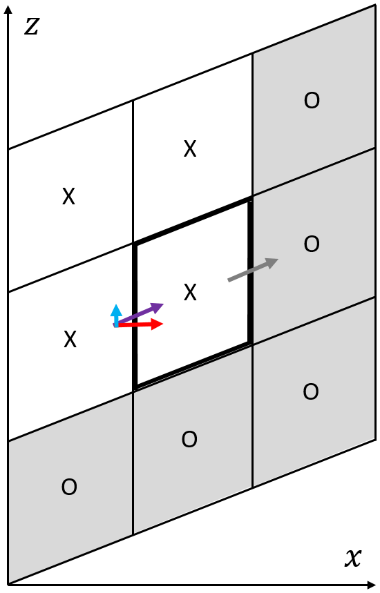
Figure 1 Example for the calculation of the diffusion in x-direction (violet and grey arrow parallel to grid cell boundaries) in a grid cell (thick black boundary) prior to model enhancements. The diffusive fluxes including the horizontal and vertical gradient of the scalar quantity are represented by the red and blue arrow. The grey arrow represents the obstacle surface flux. Obstacle cells are grey. Scalar quantities are defined at the crosses (atmospheric grid cells) and circles (building grid cells).

The diffusion is the grid following gradient $\partial /\partial {\dot{x}}^{\mathrm{1}}$ of the fluxes through the vertical grid cell boundaries (purple and grey arrow in Fig. 1). With a building at the right hand side of the grid cell, the flux is not calculated following Eq. (14). Instead, a specific building surface flux is applied (Sect. 3.2).

For the calculation of the fluxes between atmospheric grid cells, the grid following gradient $\partial /\partial {\dot{x}}^{\mathrm{1}}$ and vertical gradients of ϕ are required. The first term in brackets is represented as the violet arrow and the second as the blue arrow in Fig. 1. The calculation of the grid following $\partial /\partial {\dot{x}}^{\mathrm{1}}$ gradient of ϕ is straight forward using the values of ϕ located at the grid cell centres left and right from the grid cell boundary (crosses in the central and middle left grid cell in Fig. 1). For the calculation of the vertical gradient, however, values of ϕ from all six grid cells that surround the grid cell boundary are used (two left columns of grid cells). This includes in the example provided in Fig. 1 two building grid cells (grey), which give no physically useful values. When the horizontal diffusion is calculated, only fluxes through vertical walls are taken into account.

In general, the orography in MITRAS with the resolution of a few metres is relatively flat. Therefore, the second term in brackets in Eq. (14), which includes the slope of the terrain as $\partial {\dot{x}}^{\mathrm{3}}/\partial x$, is small. By neglecting the influence of terrain steepness in the horizontal flux, Eq. (14) simplifies to only the first term. Similar simplifications can be done for the diffusion in the y-direction. This leads to the following expressions for the horizontal turbulent fluxes:

$$\begin{array}{}\text{(15)}& {\displaystyle }-{\mathit{\rho }}_{\mathrm{0}}\stackrel{\mathrm{‾}}{u^{\prime }{\mathit{\varphi }}^{\prime }}={\mathit{\rho }}_{\mathrm{0}}{K}_{\text{hor}}{\displaystyle \frac{\partial \stackrel{\mathrm{‾}}{\mathit{\varphi }}}{\partial {\dot{x}}^{\mathrm{1}}}}{\displaystyle \frac{\partial {\dot{x}}^{\mathrm{1}}}{\partial x}}\text{(16)}& {\displaystyle }-{\mathit{\rho }}_{\mathrm{0}}\stackrel{\mathrm{‾}}{v^{\prime }{\mathit{\varphi }}^{\prime }}={\mathit{\rho }}_{\mathrm{0}}{K}_{\text{hor}}{\displaystyle \frac{\partial \stackrel{\mathrm{‾}}{\mathit{\varphi }}}{\partial {\dot{x}}^{\mathrm{2}}}}{\displaystyle \frac{\partial {\dot{x}}^{\mathrm{2}}}{\partial y}}.\end{array}$$

3.2 Changes at obstacle surfaces

Boundary fluxes had been defined before for all scalar quantities at obstacle surfaces, except for cloud, rain and snow water content. For MITRAS, those quantities are added and the treatment of building surface fluxes at obstacle surfaces is adapted for all scalar quantities.

Previously, building surface fluxes for ${\mathit{\rho }}_{\mathrm{0}}\stackrel{\mathrm{‾}}{u^{\prime }{\mathit{\varphi }}^{\prime }}$, ${\mathit{\rho }}_{\mathrm{0}}\stackrel{\mathrm{‾}}{v^{\prime }{\mathit{\varphi }}^{\prime }}$, and ${\mathit{\rho }}_{\mathrm{0}}\stackrel{\mathrm{‾}}{w^{\prime }{\mathit{\varphi }}^{\prime }}$ were defined as a three-dimensional variable located at scalar grid points. Wall orientation was taken into account in the calculation of the building surface fluxes, but when more than one building surface was present, only the value that has been calculated last was stored in the variable. For the example of a building edge as in Fig. 1, the same building surface flux was used for the vertical wall (grey arrow) as for the roof below (bottom boundary of central grid cell). Therefore, the structure of the building surface flux variables has been adjusted for all scalar quantities. Like other building surface variables (e.g. building surface temperature), a value is defined for each obstacle adjacent atmospheric grid cell and for each wall orientation. For the calculation of the pre-existing building surface fluxes, boundary conditions as described in Salim et al. (2018) and Schlünzen et al. (2018a) are applied.

For liquid water at the ground surface, the model allows for three surface boundary conditions: zero gradient, prescribed fixed value, and flux at the boundary equal to flux in the atmosphere above. For obstacle surfaces, the latter is chosen. Water and snow reaching a building close to the wall is considered to be absorbed by the adjacent surface. Considering again the configuration in Fig. 1: In order to get the building surface flux at the obstacle wall in positive x-direction of the atmospheric grid cell (grey arrow), the flux at the opposite grid cell boundary is used, calculated following Eqs. (1) and (15) (Ferner et al., 2023). The same approach is applied for other wall directions and for cloud, rain and snow water content.

4 Consideration of a snow cover scheme in MITRAS

The microscale model MITRAS' mesoscale sister model METRAS (Trukenmüller et al., 2004; Schatzmann et al., 2006; Schlünzen et al., 2018a) includes a snow cover scheme, which is described in Boettcher (2017). In the present study, a similar approach has been adapted in MITRAS. In METRAS, the snow cover scheme is only used when flux aggregation with the blending height concept is applied (von Salzen et al., 1996). In MITRAS, however, the effects of surface fractions and corresponding subgrid-scale fluxes are significantly lower due to the small grid cell sizes. Therefore, using the parameter averaging method is suitable (Schlünzen et al., 2018a) and the snow cover scheme is adapted to it. Additional adjustments are made for the consideration of obstacles, as well as for the smaller time spans and time steps of MITRAS model runs.

4.1 Surface energy budget at the ground

Without snow, the change of temperature at ground surface, T_S, with time t is calculated following Eq. (17) in MITRAS considering net short and long wave radiation SW_net and LW_net, sensible and latent heat fluxes H_S and L_S, heat flux to and from the soil at the surface G_soil (Eq. 19), using thermal diffusivity k_soil, thermal conductivity ν_soil, and deep soil temperature T_h,soil at the depth h_soil.

$$\begin{array}{}\text{(17)}& {\displaystyle \frac{\partial T_{\text{S}}}{\partial t}}=B^{*}\left({\mathrm{SW}}_{\text{net}}+{\mathrm{LW}}_{\text{net}}+H_{\text{S}}+L_{\text{S}}+G_{\text{soil}}\right)\end{array}$$

with

$$\begin{array}{}\text{(18)}& B^{*}=\mathrm{2}\sqrt{\mathit{\pi }}{\displaystyle \frac{k_{\text{soil}}}{{\mathit{\nu }}_{\text{soil}}{h}_{\text{soil}}}}\end{array}$$

The soil heat flux G_soil (Eq. 19), is expressed using the force-restore method (Bhumralkar, 1975; Deardorff, 1978). The deep soil temperature can be assumed constant for shorter time ranges (< 3 d).

$$\begin{array}{}\text{(19)}& G_{\text{soil}}=-\sqrt{\mathit{\pi }}{\left({\displaystyle \frac{h_{\text{soil}}}{{\mathit{\nu }}_{\text{soil}}}}\right)}^{-\mathrm{1}}\left(T_{\text{S}}\left(t\right)-T_{\text{h,soil}}\right)\end{array}$$

In case of snow on ground, an additional snow layer is assumed, which impacts the temperature on and near the ground surface as described for METRAS in Boettcher (2017). The treatment of the snow layer is based on Hirota et al. (2002). The thermal diffusivity of snow k_snow is given in Eq. (20) using the snow volumetric heat capacity c_v,snow (Eq. 21). The snow thermal conductivity ν_snow (Eq. 22) and volumetric heat capacity c_v,snow both depend on the density of the snow pack ρ_snow (Eq. 28). The snow thermal conductivity, the snow volumetric heat capacity, and the depth of the temperature wave into the snow are given in Eqs. (21)–(23) using the specific heat capacity of ice c_ice, the density of ice ρ_ice, the thermal conductivity of ice ν_ice, and the period of the temperature wave $\mathit{\tau }=\mathrm{86}\mathrm{400}\mathrm{s}=\mathrm{1}\mathrm{d}$.

$$\begin{array}{}\text{(20)}& {\displaystyle }{k}_{\text{snow}}={\displaystyle \frac{{\mathit{\nu }}_{\text{snow}}}{c_{\text{v,snow}}}}\text{(21)}& {\displaystyle }{c}_{\text{v,snow}}={\displaystyle \frac{c_{\text{ice}}\cdot {\mathit{\rho }}_{\text{snow}}}{{\mathit{\rho }}_{\text{ice}}}}\text{(22)}& {\displaystyle }{\mathit{\nu }}_{\text{snow}}={\mathit{\nu }}_{\text{ice}}\cdot {\left({\displaystyle \frac{{\mathit{\rho }}_{\text{snow}}}{{\mathit{\rho }}_{\text{w}}}}\right)}^{\mathrm{1.88}}\text{(23)}& {\displaystyle }{h}_{\text{snow}}=\sqrt{\mathit{\tau }\cdot {\displaystyle \frac{{\mathit{\nu }}_{\text{snow}}}{c_{\text{v,snow}}}}}\end{array}$$

The snow depth z_snow (Eq. 24) is calculated using the snow water equivalent SWE (Eq. 29) and the density of water ρ_w.

$$\begin{array}{}\text{(24)}& z_{\text{snow}}=\mathrm{SWE}\cdot {\displaystyle \frac{{\mathit{\rho }}_{\text{w}}}{{\mathit{\rho }}_{\text{snow}}}}\end{array}$$

Two cases form limit value situations which are to be treated as follows: In case of a shallow snow cover, meaning, the depth of the temperature wave into the snow h_snow (Eq. 23) exceeds the snow depth z_snow (Eq. 24), the heat conduction of snow cover and snow soil heat flux can be expressed with Eqs. (25) and (26) using Eq. (20).

$$\begin{array}{}\text{(25)}& {\displaystyle }{B}^{*}=\mathrm{2}\sqrt{\mathit{\pi }}{\displaystyle \frac{\mathrm{1}}{c_{\text{v,snow}}{z}_{\text{snow}}}}\text{(26)}& {\displaystyle }{G}_{\text{soil}}=-\sqrt{\mathit{\pi }}{\left({\displaystyle \frac{z_{\text{snow}}}{{\mathit{\nu }}_{\text{snow}}}}+{\displaystyle \frac{h_{\text{soil}}}{{\mathit{\nu }}_{\text{soil}}}}\right)}^{-\mathrm{1}}\cdot \left(T_{\text{S}}\left(t\right)-T_{\text{h,soil}}\right).\end{array}$$

In case of a very thick snow cover, the heat wave does not reach below the snow and h_soil becomes zero leading to a soil heat flux of Eq. (27) (Boettcher, 2017). The heat conduction B^* is calculated following Eq. (25) but using the temperature depth in snow h_snow instead of the snow depth z_snow.

$$\begin{array}{}\text{(27)}& G_{\text{soil}}=-\sqrt{\mathit{\pi }}{\left({\displaystyle \frac{h_{\text{snow}}}{{\mathit{\nu }}_{\text{snow}}}}\right)}^{-\mathrm{1}}\left(T_{\text{S}}\left(t\right)-T_{\text{h,soil}}\right)\end{array}$$

4.2 Snow density

As a snow pack ages, its density (Eq. 28) increases. Boettcher (2017) assumes an asymptotic solution with time from a minimum density ρ_min to a maximum density ρ_max with the empirical parameters τ_f and τ₁ and time step Δt following Verseghy (1991), Douville et al. (1995), and Dutra et al. (2010).

$$\begin{array}{}\text{(28)}& \begin{array}{rl}{\mathit{\rho }}_{\text{snow}}(t+\mathrm{\Delta }t)& =\left({\mathit{\rho }}_{\text{snow}}\left(t\right)-{\mathit{\rho }}_{\text{max}}\right)\cdot \text{exp}\left(-{\mathit{\tau }}_{\text{f}}{\displaystyle \frac{\mathrm{\Delta }t}{{\mathit{\tau }}_{\mathrm{1}}}}\right)\\ & +{\mathit{\rho }}_{\text{max}}\end{array}\end{array}$$

The parameters were chosen according to Verseghy (1991) with ${\mathit{\rho }}_{\text{min}}=\mathrm{100}{\text{kg\hspace{0.17em}m}}^{-\mathrm{3}}$, ${\mathit{\rho }}_{\text{max}}=\mathrm{300}{\text{kg\hspace{0.17em}m}}^{-\mathrm{3}}$, τ_f = 0.24 and τ₁ = 86 400 s.

For the snow albedo (Sect. 4.5), the parameters suggested by Järvi et al. (2014) were chosen in the implementation of the obstacle-resolving microscale model over those suggested by Verseghy (1991) and Boettcher (2017), as they fit observations in an urban area better by considering anthropogenic pollution. For the snow density, however, we decided to keep the parameters suggested by Verseghy (1991). The parameterisation in MITRAS is supposed to represent a snow event in a city like Hamburg (Germany). The parameters suggested by Järvi et al. (2014) fit well for snow climate cities like Montreal or Helsinki, but they do not necessarily fit equally well for Hamburg, where larger snow packs are rare.

4.3 Snow water equivalent

The snow water equivalent SWE (Eq. 29) with the unit of metres represents the mass of snow using an equivalent water height. In contrast, the height of the snow pack is given in Eq. (24). The snow water equivalent is reduced by evaporation E and melting M_snow (Eq. 30). The rate of snowfall Pr_snow adds to it (Boettcher, 2017).

$$\begin{array}{}\text{(29)}& {\displaystyle \frac{\partial \mathrm{SWE}}{\partial t}}={\mathrm{Pr}}_{\text{snow}}-E-M_{\text{snow}}\end{array}$$

In Boettcher (2017), no precipitating snow is calculated. Rain reaching the ground is assumed to be snow, if the surface temperature is below the freezing point T₀. In MITRAS, precipitating snow is calculated (Sect. 5.1) and considered in the rate of snowfall. For simplicity, rain is assumed to be snow on ground for surface temperatures below the freezing point. Similarly, precipitating snow reaching the ground for temperatures above freezing point, is assumed to be rain in the calculation of the soil water content. Diffusive fluxes into the ground are only possible in the absence of a snow cover. As a consequence, for air temperatures above freezing point, with both snow and rain falling, the snow water equivalent might be overestimated, if the surface temperatures are below the freezing point. Snow melt (Eq. 30) is calculated following Boettcher (2017) using the latent heat of fusion L₃₂.

$$\begin{array}{}\text{(30)}& M_{\text{snow}}={\displaystyle \frac{{\mathit{\nu }}_{\text{snow}}}{{\mathit{\rho }}_{\text{w}}{L}_{\mathrm{32}}{z}_{\text{snow}}}}\left(T_{\text{S}}-T_{\mathrm{0}}\right)\end{array}$$

4.4 Snow roughness length

The roughness length of snow-covered areas is reduced compared to snow-free areas as a snow pack smooths a surface. The roughness length z₀ under the influence of snow (Eq. 31) is calculated using the snow roughness length $z_{{\mathrm{0}}_{\text{snow}}}={\mathrm{10}}^{-\mathrm{3}}\text{m}$, the roughness length of areas without snow cover $z_{{\mathrm{0}}_{\text{ini}}}$, and the snow cover fraction $p_{{\text{snow}}_{{\text{z}}_{\mathrm{0}}}}$ (Eq. 32) following Boettcher (2017).

$$\begin{array}{}\text{(31)}& z_{\mathrm{0}}=(\mathrm{1}-p_{{\text{snow}}_{{\text{z}}_{\mathrm{0}}}})\cdot z_{{\mathrm{0}}_{\text{ini}}}+p_{{\text{snow}}_{{\text{z}}_{\mathrm{0}}}}\cdot z_{{\mathrm{0}}_{\text{snow}}}\end{array}$$

The parameterisation of the snow cover fraction (Eq. 32) is based on Douville et al. (1995) with the empirical factor β = 0.408.

$$\begin{array}{}\text{(32)}& p_{{\text{snow}}_{{\text{z}}_{\mathrm{0}}}}={\displaystyle \frac{\mathrm{SWE}}{\mathrm{SWE}+\mathit{\beta }\cdot z_{{\mathrm{0}}_{\text{ini}}}}}\end{array}$$

For now, the influence of snow cover on the roughness length of roofs is neglected. For obstacle surfaces including roofs, the roughness length for concrete ($z_{\mathrm{0}}={\mathrm{10}}^{-\mathrm{3}}\text{m}$) is assumed regardless of snow cover.

4.5 Snow albedo

If there is already a snow pack present, the albedo α of the ground surface (Eq. 33) is increased to a maximum albedo α_max after one hour of snowfall with the magnitude 0.01 m h⁻¹, or an equivalent value is used, e.g. with a higher magnitude for 0.01 m of snow in a shorter time (Boettcher, 2017; Dutra et al., 2010). The amount of snowfall is represented by the change of the snow water equivalent ΔSWE.

$$\begin{array}{}\text{(33)}& \begin{array}{rl}\mathit{\alpha }(t+\mathrm{\Delta }t)& =\mathit{\alpha }\left(t\right)+\text{min}\left(\mathrm{1},{\displaystyle \frac{\mathrm{\Delta }\mathrm{SWE}\cdot \mathrm{3600}\text{s}}{\mathrm{\Delta }t\cdot \mathrm{0.01}\text{m}}}\right)\\ & \cdot \left({\mathit{\alpha }}_{\text{max}}-\mathit{\alpha }\left(t\right)\right)\end{array}\end{array}$$

Baker et al. (1991) found, that a minimum snow depth of 5 cm is required to completely mask the albedo of the underlying soil. The effect of the surface covers shining through the snow surface is included in MITRAS. However, in a city like Hamburg, which aims at black roads in winter, snow rarely remains untouched because of winter services and traffic, which means the albedo of the underlying soil (α_ini) shines through for snow depths greater than 5 cm. These effects of direct human activities are included by using a basic approach. The underlying albedo is considered until a snow depth of 0.5 m is reached, then a snow cover of fresh snow is assumed. This is represented by a linear relation (Eq. 34) using the critical snow water equivalent SWE_crit = 0.05 m, which corresponds a snow depth of 0.5 m (Eq. 24). In MITRAS, Eq. (33) is used for snow albedo in case of snowfall with snow water equivalent higher than SWE_crit. Equation (34) is used for values below SWE_crit with and without snowfall because the impact of the underlying soil is assumed to be larger than the impact of aging of the snow pack.

$$\begin{array}{}\text{(34)}& \mathit{\alpha }={\mathit{\alpha }}_{\text{ini}}+\text{min}\left(\mathrm{1},{\displaystyle \frac{\mathrm{SWE}}{{\mathrm{SWE}}_{\text{crit}}}}\right)\cdot \left({\mathit{\alpha }}_{\text{max}}-{\mathit{\alpha }}_{\text{ini}}\right)\end{array}$$

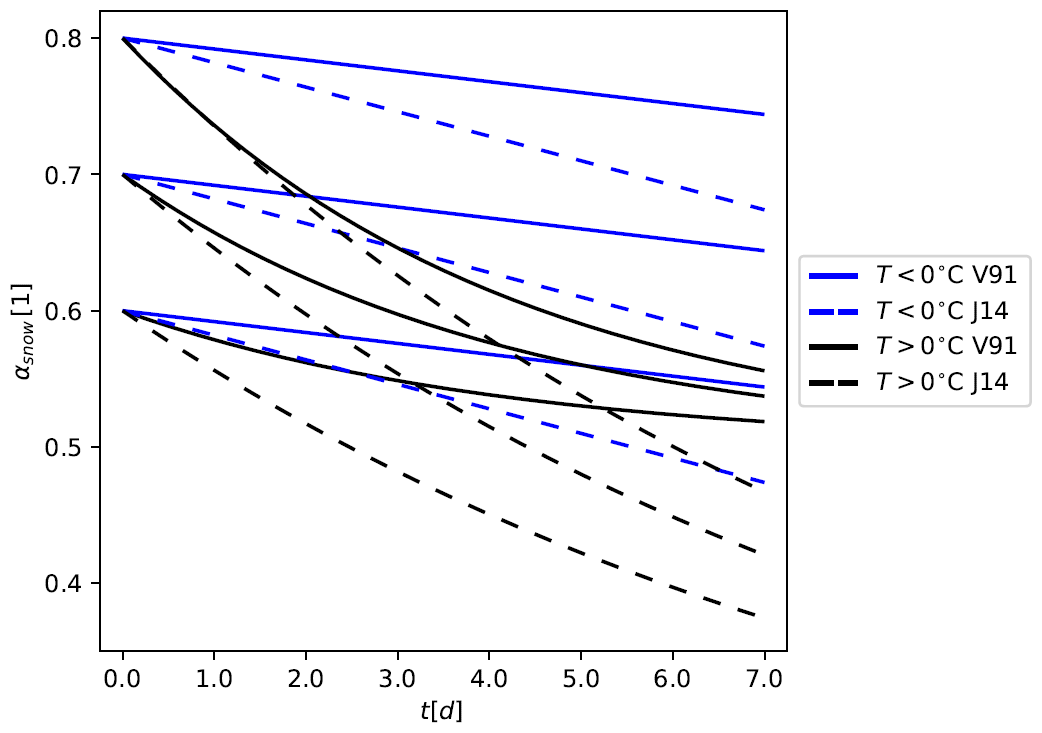
Without snowfall and a snow water equivalent greater than SWE_crit, the albedo is simultaneously decreased due to the aging of the snow pack. For temperatures below the freezing point, a linear decrease of the albedo to the minimum albedo α_min is assumed (Eq. 35) and if it is warmer, an exponential decrease (Eq. 36) is assumed using the empirical factors τ_α and τ_f,α following Verseghy (1991); Douville et al. (1995).

$$\begin{array}{}\text{(35)}& {\displaystyle }\mathit{\alpha }(t+\mathrm{\Delta }t)=\mathit{\alpha }\left(t\right)-{\mathit{\tau }}_{\mathit{\alpha }}\cdot {\displaystyle \frac{\mathrm{\Delta }t}{{\mathit{\tau }}_{\mathrm{1}}}}\text{for }{T}_{\text{S}}<\mathrm{273.16}\text{K}\text{(36)}& {\displaystyle }\begin{array}{rl}\mathit{\alpha }(t+\mathrm{\Delta }t)& =\left(\mathit{\alpha }\left(t\right)-{\mathit{\alpha }}_{\text{min}}\right)\cdot \text{exp}\left(-{\mathit{\tau }}_{\text{f},\mathit{\alpha }}\cdot {\displaystyle \frac{\mathrm{\Delta }t}{{\mathit{\tau }}_{\mathrm{1}}}}\right)\\ & +{\mathit{\alpha }}_{\text{min}}\text{for }{T}_{\text{S}}>\mathrm{273.16}\text{K}\end{array}\end{array}$$

For the mesoscale model METRAS, the parameters provided by Verseghy (1991) are applied with ${\mathit{\alpha }}_{\text{min},\text{V91}}=\mathrm{0.5}$, ${\mathit{\tau }}_{\mathit{\alpha },\text{V91}}=\mathrm{0.008}$, and ${\mathit{\tau }}_{\text{f},\mathit{\alpha },\text{V91}}=\mathrm{0.24}$ (Boettcher, 2017). However, the albedo in urban areas is generally lower than in rural areas mainly due to pollution. Järvi et al. (2014) assessed and evaluated parameters in a snow scheme for two cold climate cities (Helsinki and Montreal) and suggested the parameters: ${\mathit{\alpha }}_{\text{min},\text{J14}}=\mathrm{0.18}$, ${\mathit{\tau }}_{\mathit{\alpha },\text{J14}}=\mathrm{0.018}$, and ${\mathit{\tau }}_{\text{f},\mathit{\alpha },\text{J14}}=\mathrm{0.11}$. Both Verseghy (1991) and Järvi et al. (2014) assume a maximum snow albedo of 0.85. In Fig. 2, the decreasing albedo as described with Eqs. (35) (blue lines) and (36) (black lines) is shown for the parameters used in METRAS after Verseghy (1991) (solid lines) and the parameters based on Järvi et al. (2014) in MITRAS (dashed lines). According to Järvi et al. (2014), their suggested parameters fit well with observations in an urban area, which is why their parameters were chosen for MITRAS as well.

Figure 2 Linear (blue) and exponential (black) decrease of albedo of snow pack α_snow (Eqs. 35–36) as applied in METRAS (α_min=0.5, ${\mathit{\tau }}_{\text{f},\mathit{\alpha }}=\mathrm{0.24}$, Δt=5 s) after Verseghy (1991) (V91, solid lines) and as applied in MITRAS (α_min=0.18, ${\mathit{\tau }}_{\text{f},\mathit{\alpha }}=\mathrm{0.11}$, Δt=0.1s) after Järvi et al. (2014) (J14, dashed lines).

5 Consideration of cloud microphysics in MITRAS

The aim of extending the cloud microphysics parameterisation in MITRAS is to enable the analysis of the influence of an urban area on precipitation. Due to the very short time steps needed for numerical stability (well below 1 s) in microscale models, explicitly resolving sedimentation is necessary. This also means, that processes like accretion and sedimentation have to be taken into account during the time step calculation. The representation of a winter precipitation event is significantly improved by including an ice phase in the parameterisation. Consequently, all state-of-the-art bulk parameterisations include ice processes (Khain et al., 2015). However, currently the purpose of MITRAS is not to realistically represent the processes forming a precipitating cloud, since domain sizes are small (1 to 5 km) and thus a full formation of a cloud can only be simulated for zero wind situations and small clouds. Therefore, extending MITRAS with a comparably simple one-category ice scheme as described in Doms et al. (2011) is sufficient. There, no cloud ice is defined, but it is assumed that any cloud ice is immediately transformed to snow particles (snow $q_{\mathrm{1}}^{\mathrm{3}\text{s}}$). The ice scheme processes are shown in blue in Fig. 3.

The processes of the three-category warm rain scheme used in the M-SYS model system (Schlünzen et al., 2018a; Köhler, 1990) are provided in Sect. 2.2 and shown in grey and black in Fig. 3. In the following, the treatment of rain on roofs for MITRAS v3.1 as well as the model extension enabling the simulation of mixed-phase clouds for MITRAS v3.3 is given.

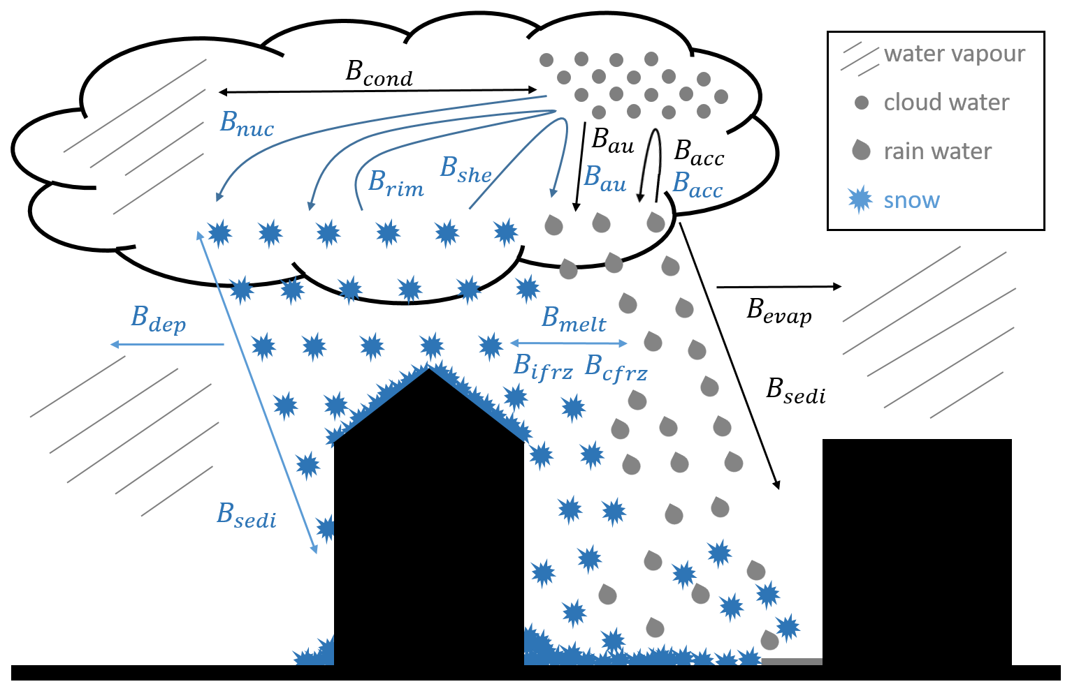
Figure 3 Cloud microphysics parameterisation with warm rain scheme in grey/black and the one-category ice scheme in blue as introduced in MITRAS.

The following balance equations describe the microphysical processes in the extended cloud scheme:

$$\begin{array}{}\text{(37)}& {\displaystyle \frac{\partial q_{\mathrm{1}}^{\mathrm{1}}}{\partial t}}=-B_{\text{cond}}+B_{\text{evap}}-B_{\text{dep}}\text{(38)}& {\displaystyle \frac{\partial q_{\mathrm{1}}^{\mathrm{2}\text{c}}}{\partial t}}=B_{\text{cond}}-B_{\text{au}}^{\text{c}}-B_{\text{nuc}}-B_{\text{acc}}^{\text{c}}-B_{\text{rim}}-B_{\text{she}}\text{(39)}& {\displaystyle }\begin{array}{rl}{\displaystyle \frac{\partial q_{\mathrm{1}}^{\mathrm{2}\text{r}}}{\partial t}}& ={\displaystyle \frac{\mathrm{1}}{{\mathit{\rho }}_{\mathrm{0}}}}{\displaystyle \frac{\partial }{\partial z}}\left({\mathit{\rho }}_{\mathrm{0}}{q}_{\mathrm{1}}^{\mathrm{2}\text{r}}{v}_{\text{TR}}\right)+B_{\text{au}}^{\text{c}}+B_{\text{acc}}^{\text{c}}+B_{\text{she}}\\ & -B_{\text{evap}}+B_{\text{melt}}-B_{\text{ifrz}}-B_{\text{cfrz}}\end{array}\text{(40)}& {\displaystyle }\begin{array}{rl}{\displaystyle \frac{\partial q_{\mathrm{1}}^{\mathrm{3}\text{s}}}{\partial t}}& ={\displaystyle \frac{\mathrm{1}}{{\mathit{\rho }}_{\mathrm{0}}}}{\displaystyle \frac{\partial }{\partial z}}\left({\mathit{\rho }}_{\mathrm{0}}{q}_{\mathrm{1}}^{\mathrm{2}\text{s}}{v}_{\text{TS}}\right)+B_{\text{nuc}}+B_{\text{rim}}+B_{\text{dep}}\\ & -B_{\text{melt}}+B_{\text{ifrz}}+B_{\text{cfrz}}\end{array}\text{(41)}& {\displaystyle }\begin{array}{rl}{\displaystyle \frac{\partial T}{\partial t}}& ={\displaystyle \frac{L_{\mathrm{21}}}{c_{\text{p}}}}{\left({\displaystyle \frac{p_{\text{S}}}{p_{\text{ref}}}}\right)}^{-\frac{R}{c_{\text{p}}}}\left(B_{\text{cond}}-B_{\text{evap}}\right)\\ & +{\displaystyle \frac{L_{\mathrm{31}}}{c_{\text{p}}}}{\left({\displaystyle \frac{p_{\text{S}}}{p_{\text{ref}}}}\right)}^{-\frac{R}{c_{\text{p}}}}{B}_{\text{dep}}+{\displaystyle \frac{L_{\mathrm{32}}}{c_{\text{p}}}}{\left({\displaystyle \frac{p_{\text{S}}}{p_{\text{ref}}}}\right)}^{-\frac{R}{c_{\text{p}}}}\left(B_{\text{nuc}}\right.\\ & \left.+B_{\text{rim}}-B_{\text{melt}}+B_{\text{ifrz}}+B_{\text{cfrz}}\right).\end{array}\end{array}$$

The balance equations are given for water vapour (Eq. 37), cloud water content (Eq. 38), rain water content (Eq. 39), snow water content (Eq. 40), and temperature (Eq. 41) with the latent heat of sublimation L₃₁, and the reference pressure p_ref = 100 000 Pa following Doms et al. (2011). Prior to the model extensions, water vapour could condensate and cloud water evaporate (Eq. 9). In the sub-saturated air below the cloud, evaporation of rain (Eq. 11) occurs and in the now extended MITRAS deposition and sublimation of snow (B_dep) as well (Sect. 5.4). The coagulation of cloud drops produces rain (autoconversion, $B_{\text{au}}^{\text{c}}$) or snow (nucleation, B_nuc) (Sect. 5.2). The accretion of rain ($B_{\text{acc}}^{\text{c}}$), riming of snow (B_rim), and shedding (B_she) by melting snow particles collecting cloud droplets thereby producing rain is included (Sect. 5.3). The first terms on the right hand sides of Eqs. (39) and (40) represent sedimentation with the terminal velocities of rain (Eq. 5) and snow (v_TS, Sect. 5.1). Melting (B_melt) as well as immersion freezing (B_ifrz) and contact nucleation (B_cfrz) of snow are now considered (Sect. 5.5). For snowflakes the Gunn-Marshall size distribution (Gunn and Marshall, 1958) is assumed.

For the radiation parameterisation in MITRAS v4.0, snow is represented as spherical droplets like rain and is added to the liquid water content within the calculation of the absorption coefficient for the long wave radiation (Sect. 2.2).

5.1 Sedimentation

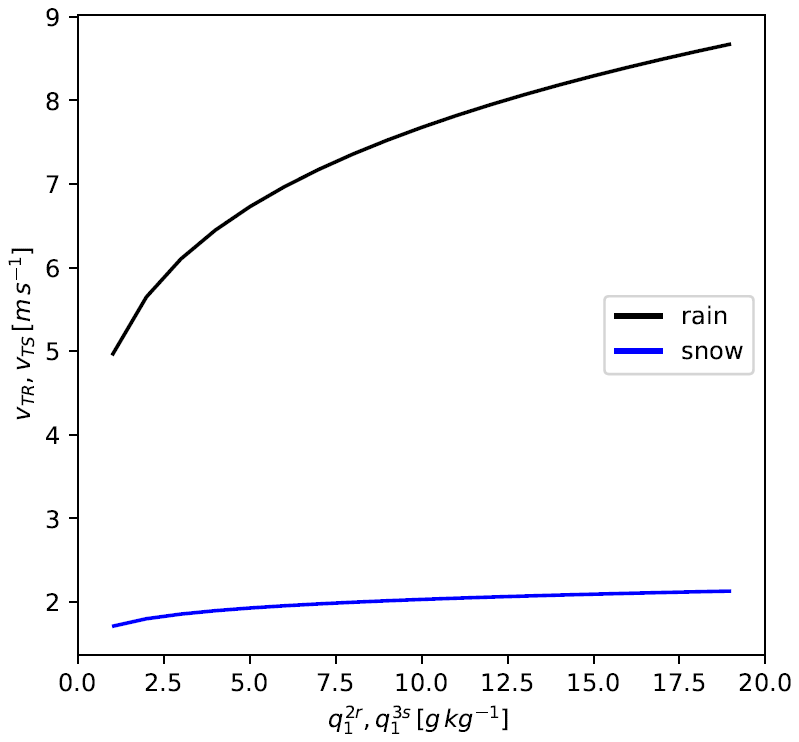
The terminal velocity for snow of

$$\begin{array}{}\text{(42)}& v_{\text{TS}}=\mathrm{4.82}\cdot {\left({\mathrm{10}}^{-\mathrm{3}}\cdot {\displaystyle \frac{{\mathit{\rho }}_{\mathrm{0}}}{{\text{kg\hspace{0.17em}m}}^{-\mathrm{3}}}}\cdot {\displaystyle \frac{q_{\mathrm{1}}^{\mathrm{3}\text{s}}}{{\text{kg\hspace{0.17em}kg}}^{-\mathrm{1}}}}\right)}^{\mathrm{0.075}}\end{array}$$

(Doms et al., 2011) is introduced. Smaller densities at higher altitudes again need to be taken into account (compare with Eq. 6). The terminal velocity of snow is lower than that of rain with a maximum value of 2.2 m s⁻¹ (blue line in Fig. 4).

Figure 4 Terminal velocities of rain v_TR (black, Eq. 5) and of snow v_TS (blue, Eq. 42) as used in MITRAS.

In general, precipitation rates and amounts are only given at ground surface in atmospheric models. In MITRAS, however, these precipitation quantities should be given on roofs as well. Precipitation quantities on roofs are calculated similar to the precipitation variables on ground (Ferner et al., 2023). For the sedimentation fluxes (first terms in Eqs. 39 and 40) in the atmosphere, the fluxes of rain and snow water content through the grid cell boundaries are calculated using the terminal velocity defined at vector points and rain and snow water content defined at grid cell centres. For the precipitation quantities at ground, a terminal velocity for the scalar point just above ground is calculated. The precipitation quantities are then derived from the flux of rain and snow above surface. In case of a roof, the terminal velocity is calculated similarly, thus using the scalar value of the terminal velocity just above the roof.

5.2 Autoconversion and nucleation

The development of snow from cloud water by subsequent diffusional growth is named nucleation. For the one-category ice scheme in MITRAS v3.3, a temperature dependence is considered:

$$\begin{array}{}\text{(43)}& \mathit{ϵ}\left(T\right)=\left\{\begin{array}{ll}\mathrm{0}& \text{if }T\ge T_{\mathrm{0}}\\ \mathrm{0.5}\left[\mathrm{1}+\text{sin}\left(\frac{\mathit{\pi }\cdot \left(\mathrm{0.5}\left(T_{\mathrm{0}}+T_{\mathrm{2}}\right)-T\right)}{T_{\mathrm{0}}-T_{\mathrm{2}}}\right)\right]& \text{if }{T}_{\mathrm{2}}<T<T_{\mathrm{0}}\\ \mathrm{1}& \text{if }T\le T_{\mathrm{2}}.\end{array}\right.\end{array}$$

According to Doms et al. (2011), it is based on observations of the frequency distribution of water and ice in mixed-phase clouds. ϵ(T) is one below the minimum temperature T₂ = 235.16 K and zero above the freezing point (T₀). Note, that the conversion coefficient for Kelvin in MITRAS is 273.16 and not 273.15 as in (Doms et al., 2011).

The conversion rates are given as

$$\begin{array}{}\text{(44)}& {\displaystyle }{B}_{\text{au}}^{\text{c}}=\text{max}(\mathrm{0},k_{\text{cold}}^{\text{r}}\cdot \left(\mathrm{1}-\mathit{ϵ}\left(T\right)\right)\cdot \left(q_{\mathrm{1}}^{\mathrm{2}\text{c}}-q_{\mathrm{1},\text{cri}}^{\mathrm{2}\text{c}}\right)\text{(45)}& {\displaystyle }{B}_{\text{nuc}}=\text{max}(\mathrm{0},k_{\text{cold}}^{\text{s}}\cdot \mathit{ϵ}(T)\cdot \left(q_{\mathrm{1}}^{\mathrm{2}\text{c}}-q_{\mathrm{1},\text{cri}}^{\mathrm{2}\text{c}}\right)\end{array}$$

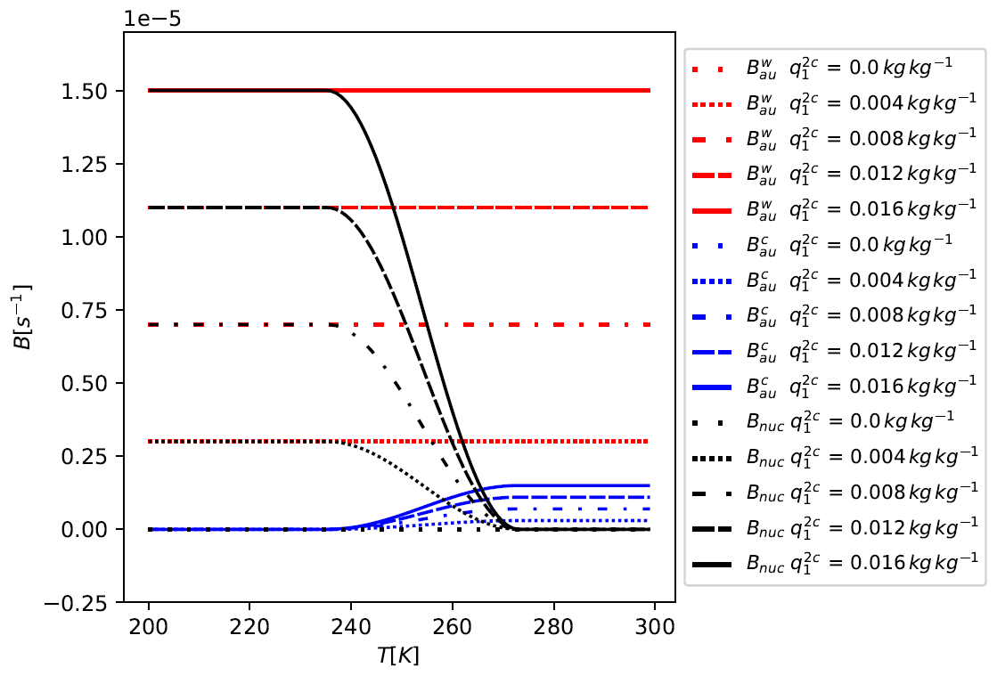
with the autoconversion interval for rain $k_{\text{cold}}^{\text{r}}={\mathrm{10}}^{-\mathrm{4}}{\text{s}}^{-\mathrm{1}}$ and for snow $k_{\text{cold}}^{\text{s}}={\mathrm{10}}^{-\mathrm{3}}{\text{s}}^{-\mathrm{1}}$ (Doms et al., 2011). Note, that unlike in Doms et al. (2011), a nonzero value for $q_{\mathrm{1},\text{cri}}^{\mathrm{2}\text{c}}$ is chosen in MITRAS. In Fig. 5 the autoconversion rates for warm clouds (Eq. 7, red) and mixed phase clouds (Eq. 44, blue) are shown as well as the nucleation rates (Eq. 45, black). All processes increase with increasing cloud water contents. While the autoconversion in the warm rain scheme only depends on the cloud water content, the other processes additionally depend on temperature. When mixed-phase clouds are assumed, less rain water is created by autoconversion than in warm clouds for the same cloud water content. Below T₂=235.16 K the nucleation of snow is highest and the autoconversion is zero. The nucleation gradually decreases and the autoconversion increases with higher temperatures until the freezing point is reached.

Figure 5 Autoconversion rates for warm clouds (red, $B_{\text{au}}^{\text{w}}$, Eq. 7) and mixed phase clouds (blue, $B_{\text{au}}^{\text{c}}$, Eq. 44) and nucleation rates (black, B_nuc, Eq. 45) for different cloud water contents $q_{\mathrm{1}}^{\mathrm{2}\text{c}}$ and temperatures T.

5.3 Accretion and riming

For riming, the continuous model for particle growth by collection is applied. Snow particles have no spherical shapes. Instead, they are assumed to be rimed aggregates of crystals and they have the form of thin circular plates. The temperature dependent mass-size relation of snow is defined as

$$\begin{array}{}\text{(46)}& \begin{array}{rl}& a_{\text{m}}\left(T\right)=\\ & \left\{\begin{array}{ll}{a}_{\text{mc}}-a_{\text{mv}}\left[\mathrm{1}+\text{cos}\left\{\frac{\mathrm{2}\mathit{\pi }\left(T-\mathrm{0.5}(T_{\mathrm{0}}+T_{\mathrm{1}})\right)}{\left(T_{\mathrm{0}}-T_{\mathrm{1}}\right)}\right\}\right]& \text{if }{T}_{\mathrm{0}}>T>T_{\mathrm{1}}\\ a_{\text{mc}}& \text{else}\end{array}\right.\end{array}\end{array}$$

with the constant parameters $a_{\text{mc}}=\mathrm{0.08}{\text{kg\hspace{0.17em}m}}^{-\mathrm{2}}$ and $a_{\text{mv}}=\mathrm{0.02}{\text{kg\hspace{0.17em}m}}^{-\mathrm{2}}$ and the temperature T₁ = 253.16 K (Doms et al., 2011).

For the accretion term (Eq. 8) in the one-category ice scheme, the temperature dependency (Eq. 43) is considered:

$$\begin{array}{}\text{(47)}& {\displaystyle }\begin{array}{rl}{B}_{\text{acc}}^{\text{c}}& =(\mathrm{1}-\mathit{ϵ}(T\left)\right)\cdot \mathrm{934.63}\cdot {\displaystyle \frac{q_{\mathrm{1}}^{\mathrm{2}\text{c}}}{{\text{kg\hspace{0.17em}kg}}^{-\mathrm{1}}}}\\ & \cdot {\left({\displaystyle \frac{{\mathit{\rho }}_{\mathrm{0}}}{{\text{kg\hspace{0.17em}m}}^{-\mathrm{3}}}}\times {\mathrm{10}}^{-\mathrm{3}}\cdot {\displaystyle \frac{q_{\mathrm{1}}^{\mathrm{2}\text{r}}}{{\text{kg\hspace{0.17em}kg}}^{-\mathrm{1}}}}\right)}^{\mathrm{0.875}}\end{array}\text{(48)}& {\displaystyle }\begin{array}{rl}& B_{\text{rim,MITRAS}}=\\ & \left\{\begin{array}{ll}{\left(\frac{a_{\text{m}}\left(T\right)}{{\text{kg\hspace{0.17em}m}}^{-\mathrm{2}}}\right)}^{-\mathrm{1}}\cdot \mathrm{3307.24}\cdot \frac{q_{\mathrm{1}}^{\text{2c}}}{{\text{kg\hspace{0.17em}kg}}^{-\mathrm{1}}}& \\ \cdot {\left(\frac{{\mathit{\rho }}_{\mathrm{0}}}{{\text{kg\hspace{0.17em}m}}^{-\mathrm{3}}}\times {\mathrm{10}}^{-\mathrm{3}}\cdot \frac{q_{\mathrm{1}}^{\text{3s}}}{{\text{kg\hspace{0.17em}kg}}^{-\mathrm{1}}}\right)}^{\mathrm{1.075}}& \text{if }T<T_{\mathrm{0}}\\ \mathrm{0}& \text{if}T\ge T_{\mathrm{0}}.\end{array}\right.\end{array}\end{array}$$

Otherwise it remains the same as in MITRAS v3.0. Note, that (Doms et al., 2011) uses different parameters for the accretion.

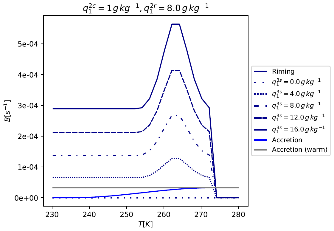
Figure 6 The riming rates (Eq. 48, dark blue) with the cloud water content of $q_{\mathrm{1}}^{\mathrm{2}\text{c}}=\mathrm{1}\times {\mathrm{10}}^{-\mathrm{3}}{\text{kg\hspace{0.17em}kg}}^{-\mathrm{1}}$ for various snow water contents $q_{\mathrm{1}}^{\mathrm{3}\text{s}}$ depending on the temperature T and the accretion rates for $q_{\mathrm{1}}^{\mathrm{2}\text{c}}=\mathrm{1}\times {\mathrm{10}}^{-\mathrm{3}}{\text{kg\hspace{0.17em}kg}}^{-\mathrm{1}}$ and the rain water content $q_{\mathrm{1}}^{\mathrm{2}\text{r}}=\mathrm{8}\times {\mathrm{10}}^{-\mathrm{3}}{\text{kg\hspace{0.17em}kg}}^{-\mathrm{1}}$ for the mixed-phased cloud parameterisation as used in MITRAS v3.3 (Eq. 47, light blue) and warm cloud parameterisation as used in MITRAS v3.0 (Eq. 8, grey).

In Fig. 6, the accretion rates for the warm rain parameterisation used in MITRAS v3.0 (grey) and the mixed-phase cloud parameterisation as used in MITRAS v4.0 (light blue) is shown as well as the riming rates (dark blue). Accretion increases for rain for temperatures above T₂ (Eq. 43) reaching the same value as warm clouds at the freezing point T₀. The riming rate is highest at −10 °C, as the largest snowflakes can be found at −10 °C (Eq. 46). Snow production is higher than rain production for the same initial snow respectively rain amount. At temperatures below the freezing point T₀, snow is produced by riming. If it is warmer, rain water content is produced by shedding. The equation is the same as riming (Eq. 48), but it produces rain water and not snow.

5.4 Depositional growth

With the inclusion of snow, depositional growth (diffusion growth of snow particles) and sublimation occur, which is according to Doms et al. (2011) given as

$$\begin{array}{}\text{(49)}& \begin{array}{rl}{B}_{\text{dep}}& ={\displaystyle \frac{{\mathit{\alpha }}_{\text{dep}}}{{\left(a_{\text{m}}\left(T\right)\right)}^{\mathrm{0.5}}}}\left(\mathrm{1}+{\displaystyle \frac{{\mathit{\beta }}_{\text{dep}}}{{\left(a_{\text{m}}\left(T\right)\right)}^{\mathrm{0.25}}}}{\left({\mathit{\rho }}_{\mathrm{0}}{q}_{\mathrm{1}}^{\mathrm{3}\text{s}}\right)}^{\mathrm{0.225}}\right)\\ & \left(q_{\mathrm{1}}^{\mathrm{1}}-q_{\mathrm{1},\text{sat},\text{ice}}^{\mathrm{1}}\right){\left({\mathit{\rho }}_{\mathrm{0}}{q}_{\mathrm{1}}^{\mathrm{3}\text{s}}\right)}^{\mathrm{0.625}}\end{array}\end{array}$$

with the factors

$$\begin{array}{}\text{(50)}& {\mathit{\alpha }}_{\text{dep}}=\left(\mathrm{1.09}\times {\mathrm{10}}^{-\mathrm{3}}-\mathrm{3.34}\times {\mathrm{10}}^{-\mathrm{5}}\left(T-T_{\mathrm{0}}\right)\right)\end{array}$$

and β_dep = 13.0. $q_{\mathrm{1},\text{sat},\text{ice}}^{\mathrm{1}}$ denotes the saturation specific humidity over ice. For better readability, the units of α_dep and β_dep are not provided here. They can be found in Doms et al. (2011).

5.5 Melting and freezing

The melting rate is derived similarly to the evaporation and deposition rates leading to

$$\begin{array}{}\text{(51)}& \begin{array}{rl}{B}_{\text{melt}}& ={\displaystyle \frac{{\mathit{\alpha }}_{\text{melt}}}{a_{\text{mc}}^{\mathrm{0.5}}}}\left(\mathrm{1}+{\mathit{\beta }}_{\text{melt}}{a}_{\text{mc}}^{\mathrm{0.25}}{\left({\mathit{\rho }}_{\mathrm{0}}{q}_{\mathrm{1}}^{\mathrm{3}\text{s}}\right)}^{\mathrm{0.225}}\right)\\ & \left(T-T_{\mathrm{0}}\right){\left({\mathit{\rho }}_{\mathrm{0}}{q}_{\mathrm{1}}^{\mathrm{3}\text{s}}\right)}^{\mathrm{0.625}}\end{array}\end{array}$$

with the factors ${\mathit{\alpha }}_{\text{melt}}=\mathrm{7.2}\times {\mathrm{10}}^{-\mathrm{6}}$ and β_melt = 13.0 (Doms et al., 2011).

Rain drops can be activated as ice nuclei due to various drop impurities (immersion freezing), this is represented in the model as

$$\begin{array}{}\text{(52)}& {\displaystyle }{B}_{\text{ifrz}}={\displaystyle }{\mathit{\alpha }}_{\text{if}}\left(e^{{\mathit{\alpha }}_{\text{if}}(T_{\mathrm{0}}-T)}-\mathrm{1}\right){\left({\mathit{\rho }}_{\mathrm{0}}{q}_{\mathrm{1}}^{\mathrm{2}\text{r}}\right)}^{\mathrm{1.75}}\end{array}$$

with the parameter ${\mathit{\alpha }}_{\text{if}}=\mathrm{9.95}\times {\mathrm{10}}^{-\mathrm{5}}$ (Doms et al., 2011).

The process of falling rain drops collecting ice nuclei (contact freezing nucleation) is represented as

$$\begin{array}{}\text{(53)}& \begin{array}{rl}& B_{\text{cfrz}}=\\ & \left\{\begin{array}{ll}{\mathit{\alpha }}_{\text{cf}}{E}_{\text{cf}}{N}_{\text{cf},\mathrm{0}}(\mathrm{270.17}-T{)}^{\mathrm{1.3}}({\mathit{\rho }}_{\mathrm{0}}{q}_{\mathrm{1}}^{\text{2r}}{)}^{\mathrm{1.625}}& \text{if }T<\mathrm{270.17}\text{K}\\ \mathrm{0}& \text{if }T\ge \mathrm{270.17}\text{K}\end{array}\right.\end{array}\end{array}$$

with the parameter ${\mathit{\alpha }}_{\text{cf}}=\mathrm{1.55}\times {\mathrm{10}}^{-\mathrm{3}}$, the collection efficiency $E_{\text{cf}}=\mathrm{5.0}\times {\mathrm{10}}^{-\mathrm{3}}$, and the concentration of natural contact ice nuclei active at −4 °C at sea level $N_{\text{cf},\mathrm{0}}=\mathrm{2.0}\times {\mathrm{10}}^{\mathrm{5}}$ (Doms et al., 2011). Again, the units can be found in Doms et al. (2011).

6 Validation

Previous versions of MITRAS are confirmed to represent well the main atmospheric features within an urban boundary layer. MITRAS v1.0 has been validated in comparison to wind tunnel data (Schlünzen et al., 2003; Grawe et al., 2013). MITRAS v2.0 (Salim et al., 2018) has been evaluated using the VDI guideline for microscale, obstacle-resolving models (Grawe et al., 2015). The model extensions concerning radiation in MITRAS v3.0 are described and validated in Fischereit (2018). As most parts of the extended model are already validated (e.g. Ferner et al., 2023), an assessment of the plausibility of the model results is performed here. Furthermore, tests in comparison to measured data are challenging, because in a model domain of this size hardly any high-resolution in-situ data are available.

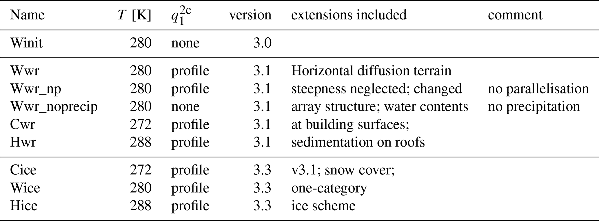
For a more in depth assessment of the winter parameterisations introduced in the current paper, model results achieved by using different model versions are compared using “to be expected outcomes” for an assessment. The set-ups of the simulations and corresponding model version number are listed in Table 1. MITRAS v3.0 is considered to be the initial version (index “init” in name). MITRAS v3.1 (index “wr”) includes neglecting the influence of terrain steepness on horizontal diffusion terms (Sect. 3.1), changing the structure of all scalar obstacle surface variables and introduction of boundary conditions at obstacle surfaces for water content variables (Sect. 3.2), and sedimentation of rain on roofs (Sect. 5.1). In a previous study, MITRAS v3.1 has been tested with focus on the reliability of the rain processes in comparison with in-situ rain radar data (Ferner et al., 2023). MITRAS v3.3 includes the winter precipitation scheme (use denoted by index “ice” in Table 1) described in Sects. 4 and 5.

Table 1 Set-up for simulations with different initial surface temperatures T (W for warm, C for cold, H for hot), cloud water contents $q_{\mathrm{1}}^{\mathrm{2}\text{c}}$, and development stage of the model. For details see text.

6.1 Model set-up

All simulations are performed for the same model domain (Sect. 6.2). For the plausibility tests in Sect. 6.4, simulations with three different initial surface level temperatures (“C” for cold, “W” for warm, “H” for hot in Table 1) are performed. In Fig. 7, the initial temperature profiles are provided in black. For the profile, a potential temperature gradient of 0.001 K m⁻¹ is assumed. For all simulations except Winit and Wwr_noprecip, nonzero initial cloud water contents (blue solid line in Fig. 7) are prescribed which lead to heavy precipitation. The initial surface level pressure is 990 hPa, the initial wind at 150 m a.g.l. is from west (2 m s⁻¹). Due to Coriolis force effects, the wind direction at 10 m height is south west with a friction reduced wind speed of 1.2 m s⁻¹. The initial relative humidity is set to 60 % at ground and reduces to 30 % at the top of the model domain (5 km) yielding the specific humidity profiles in Fig. 7 (dash-dotted, dashed, dotted blue lines). At the lateral boundaries and at the upper boundary a gradient of zero is assumed except for boundary normal winds, where boundary values are either calculated (lateral) or large-scale values are prescribed (top). At the bottom boundary for wind fixed values are prescribed. For temperature and specific humidity, the surface energy budget is calculated (Sect. 4) and for cloud, rain, and snow water content, the flux at the boundary equals the flux in the model (Sect. 3.2).

The plausibility tests are performed using hit rates (Sect. 6.3). To determine them, allowed uncertainty ranges have to be found for the meteorological variables. This is based on published methods to asses obstacle-resolving model performance and is done for variables by comparing model results with and without parallelisation (Wwr and Wwr_np in Table 1).

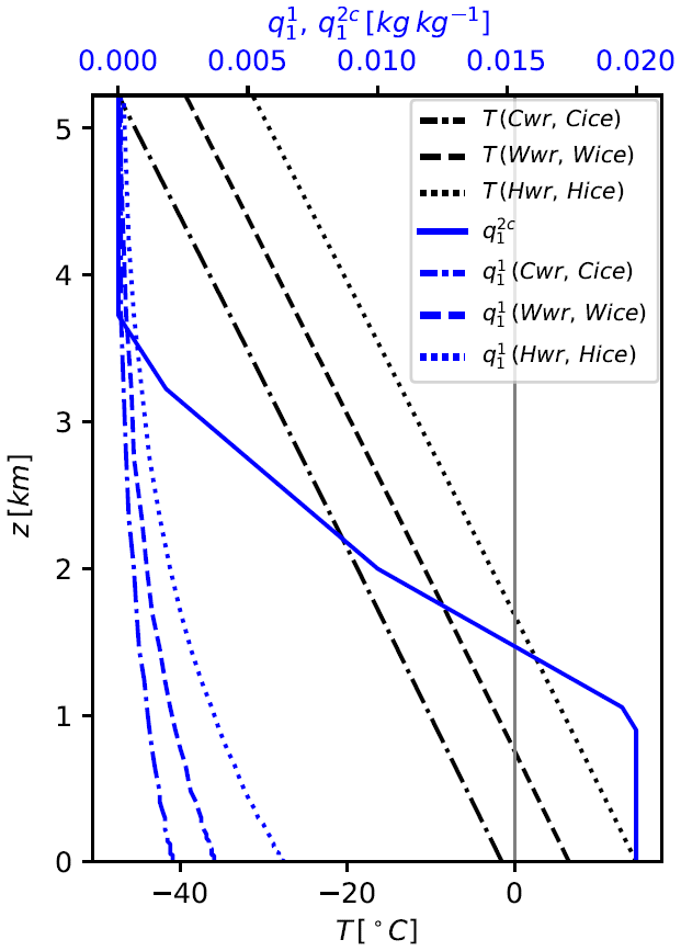
Figure 7 Initial temperature (black), specific humidity $q_{\mathrm{1}}^{\mathrm{1}}$ and cloud water content $q_{\mathrm{1}}^{\mathrm{2}\text{c}}$ (both blue) vertical profiles for cold (dashdotted line), warm (dashed line), and hot cases (dotted line). The cloud water content profile (solid line) is identical for all cases that include precipitation. The grey line denotes the freezing point.

6.2 Model domain

The model domain is small to ensure a fast integration. However, it includes orography, slanted roofs, obstacle corners and different surface cover classes to assess, if the model can represent the different features for a realistic urban area. The domain extends 240 m × 210 m horizontally and 6400 m vertically with an equidistant area of 3 m resolution in the middle (Fig. 8). The grid increases towards the lateral boundaries to a maximum horizontal resolution of 10 m. The maximum vertical resolution of 500 m is achieved at 3 km a.g.l. Typically, domains of obstacle-resolving models extend only few hundred metres vertically (Geletič et al., 2022; Grawe et al., 2013). However, with interest in cloud and precipitation development in the influence of a building, the upper level is chosen high enough to ensure a vertical extension of clouds is not hindered by a too low model top. Grid sizes increase in horizontal as well as vertical direction by a factor of 1.175. The equidistant area ranges from −28 to 26 m in the x-direction and −16 to 18 m in the y-direction and from the ground up to 32 m.

A single building with roof heights at 15 and 10 m, and a size of 45 m by 45 m (Fig. 9) including edges and slanted surfaces is placed on top a small mound. This setup resembles a terp, which is a North European form of housing, where an artificial mound protects the building from flooding. At the boundaries is cropland. The pavement and the streets are made of asphalt. At obstacles, the surface cover class is concrete (Fig. 10). The simulations start at 7:30 and finish at 8:32. Within this time span, a precipitation event takes place and the sun rises. The focus area of the analyses lies in the centre of the domain (dashed lines in Figs. 8 and 10).

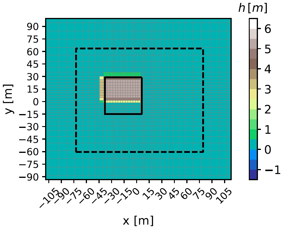
Figure 8 Orography height h (shaded) of model domain. The solid line denotes the contour of the building and the black dashed line the model domain taken into account in the result analyses. Thin lines illustrate the horizontal grid.

Figure 9 Roof height bh.

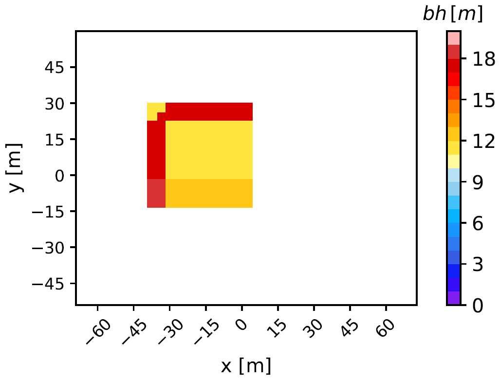
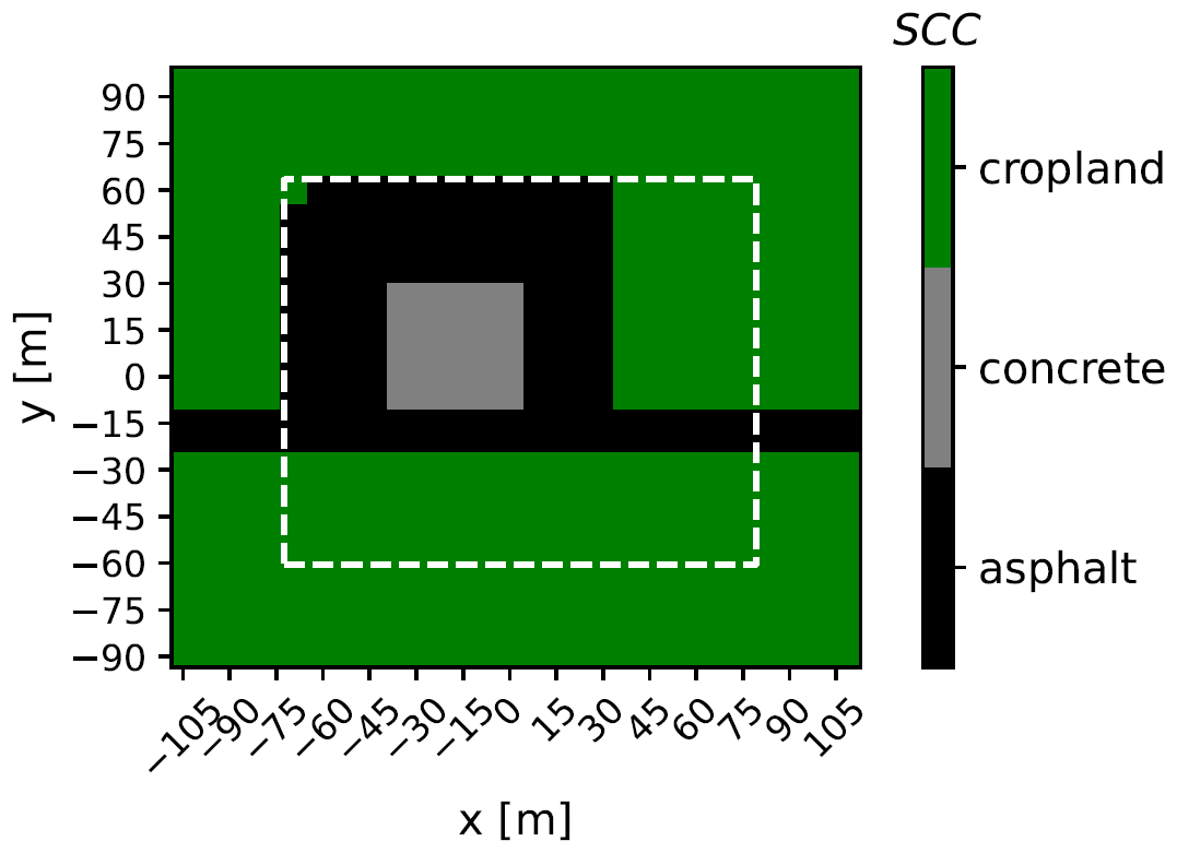
Figure 10 Surface cover classes. The dashed line denotes the model domain taken into account in the result analyses.

6.3 Derivation of model uncertainty values

The assessment, whether model results are identical or different is based on a method described in VDI (2017) which uses hit rates. Hit rates have been applied in the past for assessing microscale models (e.g. Eichhorn and Kniffka, 2010; Franke et al., 2012; Grawe et al., 2013). as well as for other model scales (e.g. weather forecast (Cox et al., 1998), mesoscale air quality and meteorology models (Schlünzen and Sokhi, 2008)). The hit rate q is defined as:

$$\begin{array}{}\text{(54)}& q={\displaystyle \frac{\mathrm{1}}{N}}\sum _{i=\mathrm{1}}^N{n}_i\end{array}$$

with N being the total number of compared values and n_i equal 1 (hit) or 0 (fail) depending on the deviation of model results and comparison data:

$$\begin{array}{}\text{(55)}& n_i=\left\{\begin{array}{ll}\mathrm{1}& \text{if }\left|\frac{{\mathrm{Pd}}_i-O_i}{O_i}\right|\le D\text{ or }\left|{\mathrm{Pd}}_i-O_i\right|\le W\\ \mathrm{0}& \text{else}.\end{array}\right.\end{array}$$

For every atmospheric grid cell at location i, the wind speed is assessed per component (u, v, w). The comparison results in a hit (n_i = 1), if the relative deviation does not exceed the threshold value, D, or the absolute deviation remains below the corresponding threshold W. When comparing model results to observational data, Pd_i denotes the predicted and O_i the observed values. In the present study, results of different model versions are compared. Pd_i denotes the newer model version and O_i the older version. Following VDI (2017) and WMO (2023), a hit rate of q ≥ 95 % between two simulation results are considered similar. There, the threshold values for absolute and relative deviations, W and D, for the wind speed components speeds are $W_{\text{VDI}}=\mathrm{0.01}{\text{m\hspace{0.17em}s}}^{-\mathrm{1}}$ and D_VDI = 0.05. Wind speed components are normalised with the reference wind speed U_ref for the test cases. In the current study, the initial wind speed of 2 m s⁻¹ is used as reference wind speed. As non-normalised values are compared, W has to be adjusted to $W=W_{\text{VDI}}\cdot U_{\text{ref}}=\mathrm{0.02}{\text{m\hspace{0.17em}s}}^{-\mathrm{1}}$ (Table 2). For the relative deviation, D_VDI is assumed for D for each of the wind speed components (Table 2). It should be noted that these values are about a factor of 10 smaller than the required measurement uncertainties for wind speed given in WMO (2023).

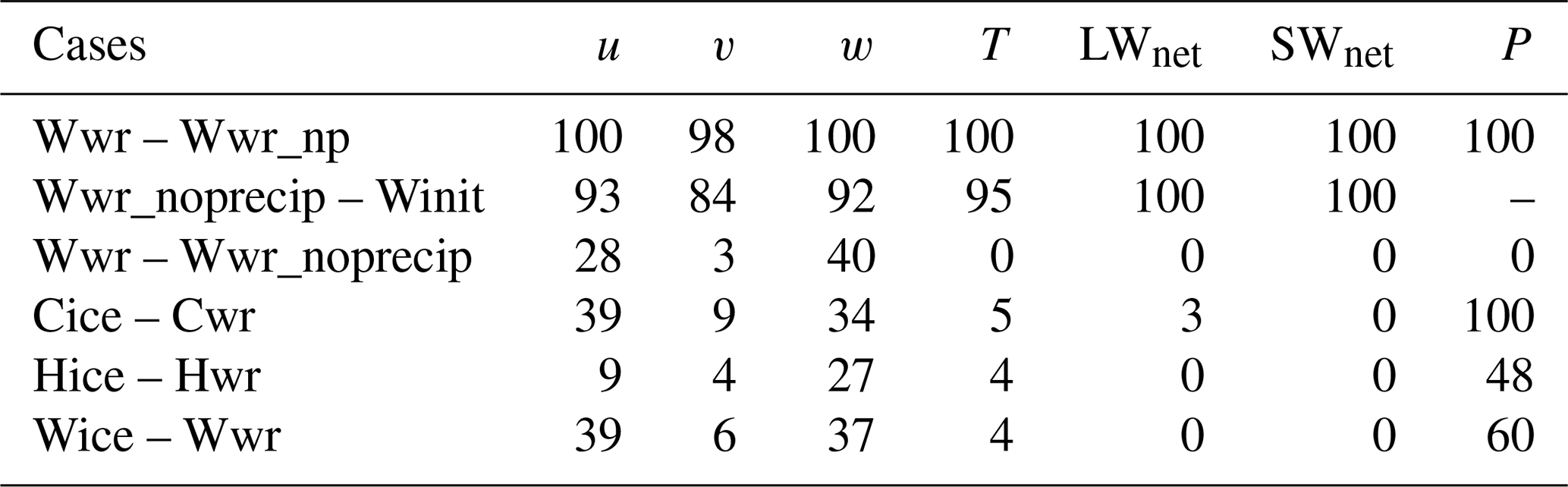
In this study, not only the results for the components of the wind vector but also the results for temperature, long and short wave radiation, and precipitation amount on ground P are assessed. The W and D values for these meteorological variables are derived by comparing the results of MITRAS v3.0 with one running in parallel processing mode and the other one with single processor use (with and without parallelisation; Wwr and Wwr_np) after one hour of simulation. This measure is taken, since the same model might yield different results depending on compilers, installed packages, and hardware. Therefore, hit rates below 100 % can occur (e.g. 98 % for v, Table 3). As a hit rate above 95 % means the results lie within the required accuracy, Wwr and Wwr_np can be considered identical (Table 3).

With computational accuracy a strict criterion is applied for temperature, radiation, and precipitation. The resulting W and D values are consistent with the allowed uncertainty values for the wind speed components, as they also are about a factor of 10 smaller than given in WMO (2023). For example, the achievable uncertainty for temperature suggested by WMO (2023) is 0.2 K and here 0.05 K is chosen. For long and short wave radiation $\mathrm{1}/\mathrm{10}$th of the values for direct solar radiation (4–6 W m⁻² WMO, 2023) is used. The allowed absolute deviation of 0.001 mm for precipitation is well below the accuracy of commonly used rain gauges (0.1 mm, WMO, 2023). This strict value is chosen because precipitation is the target value of our model extensions. Low hit rates give the impression of larger differences. It should be noted that the dependency of the hit rate on the allowed deviations is a shortcoming of this validation metric as discussed in Franke et al. (2012). We use this dependency to our advantage. The comparison of results of different model versions (e.g. with/without parallelisation, code extensions used with values of zero for the variables) should lead to very similar results. In contrast, extensions of a model with new or changed process descriptions and nonzero values for variables should provide different model results and thus small hit rates.

Table 2 Thresholds for the absolute (W) and relative deviation (D) for hit rate calculation (q) for wind speed components u, v, w, temperature T, net long and short wave radiation LW_net and SW_net, and precipitation amount P on ground. For details on their derivation see text.

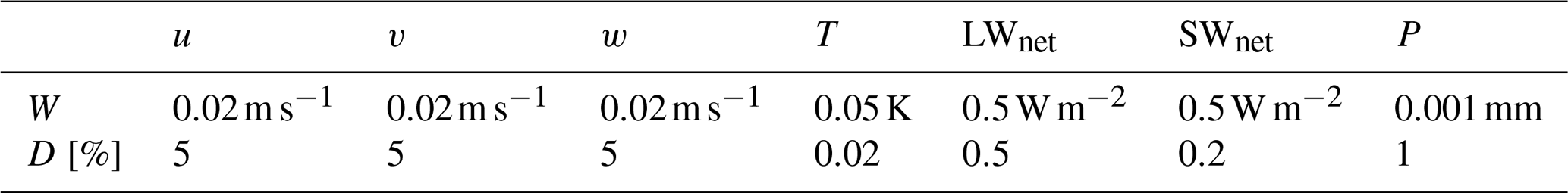
Table 3 Hit rates q in percent of wind components (u, v, w), temperature (T), net surface long wave and short wave radiation (LW_net SW_net), and precipitation amount (P) on ground after 1 h simulation time.

6.4 Model plausibility and functionality

6.4.1 Influences of the modifications of the diffusion

The comparison of the results from simulations using MITRAS v3.1 (Wwr_noprecip) with simulations using MITRAS v3.0 (Winit) for dry atmospheric conditions would show any influences of changes due to the calculation of the horizontal diffusion of scalars (Sect. 3.1) and the modified structure for all scalar quantities at obstacle surfaces (Sect. 3.2). The changes of the model physics by the modifications in horizontal diffusion are small, but due to the strictness of the required accuracy, a good agreement with hit rates of 95 % is not expected for the whole domain. As the effects of slopes are largest close to the ground surface, the largest discrepancies are to be expected there. Not surprisingly, hit rates are below 95 % for the wind speed components (Table 3). The results for temperature, long and short wave radiation can be considered identical. The lowest hit rate in this comparison of 84 % is found for the lateral wind component v. Misses are only found in grid cells near the ground (Fig. 11), where the terrain steepness of the terrain-following coordinate system has the most effect, which is plausible.

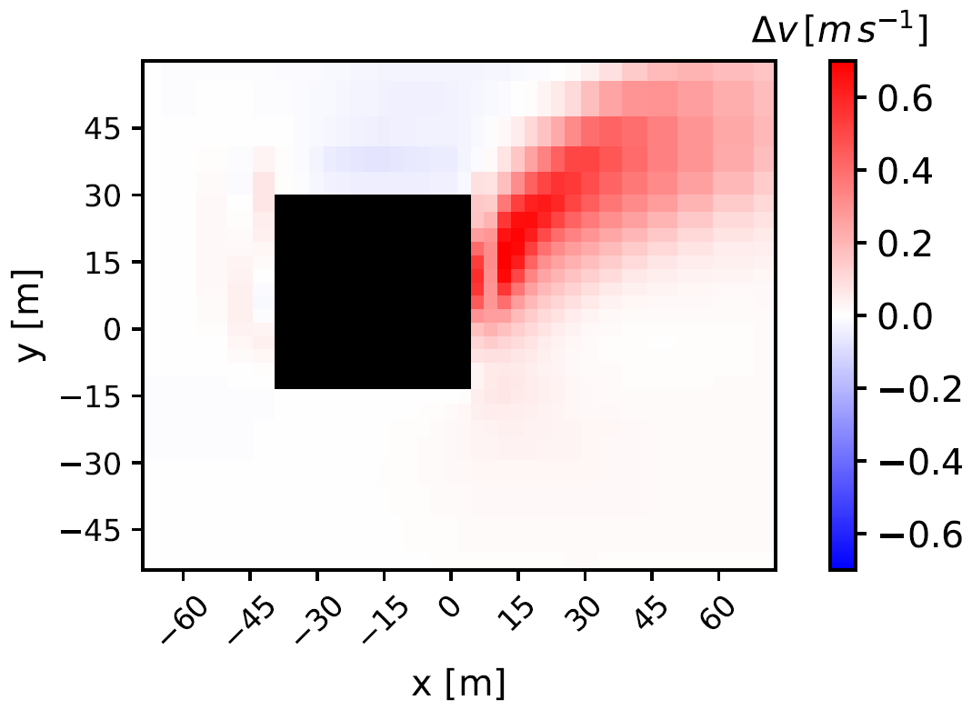
Figure 11 Difference of v-wind component Δv of Wwr_noprecip and Winit at 1.5 m height at 08:32:00 LST.

6.4.2 Influences of cloud formation

The influence of the presence of atmospheric liquid water on the radiation is included in MITRAS v3.1. When liquid water is present, shading by clouds is considered using the two-stream approach instead of the vertically integrated radiation approach (Sect. 2.2). This leads to different net surface radiations. Comparing simulations with and without precipitation (Wwr and Wwr_noprecip) therefore reveals, not surprisingly, profound differences with hit rates below 40 % for all meteorological variables with the flow field being more similar than the temperature, short and long wave radiation and precipitation (Table 3). Without precipitation, the shadow cast by the building and the reflection by the small elevation can be seen very clearly in the net surface short wave radiation (not shown). This effect is not as pronounced when cloud water is present as the cloud blocks the radiation. However, the differences still show the direct shading by building and slope (Fig. 12). With and without liquid water, the net surface long wave radiation is negative meaning the net flux is outward. However, the absolute values are larger without liquid water in the atmosphere (not shown) as there is less backscattering and surfaces get warmer. These results confirm Ferner et al. (2023), where results of MITRAS v3.1 were compared with in-situ measurements and the model has been shown to produce plausible results.

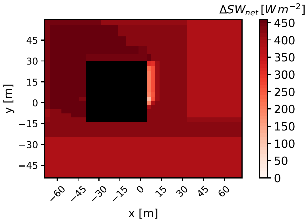
Figure 12 Difference of net surface short wave radiation ΔSW_net of Wwr and Wwr_noprecip at 08:32:00 LST.

6.4.3 Influences of snow cover

By including snow cover (Sect. 4) in MITRAS v3.3, the homogenising effect of snow cover on the albedo is represented in the model. The snow cover parameterisation is implemented in Cice and the temperature is sufficiently low for snow to reach the ground and remain. Without snow cover, most of the focus area is asphalt (Fig. 10) with an albedo of 0.09. Cropland has an albedo of 0.2. Without snow cover (case Cwr), the median of the albedo therefore is 0.09. This can be seen in Fig. 13, where box plots of albedo values of cases Cice (grey, MITRAS v3.3) and Cwr (blue, MITRAS v3.1) are shown. For Cwr, the box plots remain the same over time. With snow cover (Case Cice), the median increases with increasing snow cover, while the spread of the albedo data decreases. The albedo does not reach the maximal snow albedo of 0.85 (Sect. 4.5), meaning that underlying soil still slightly shines through.

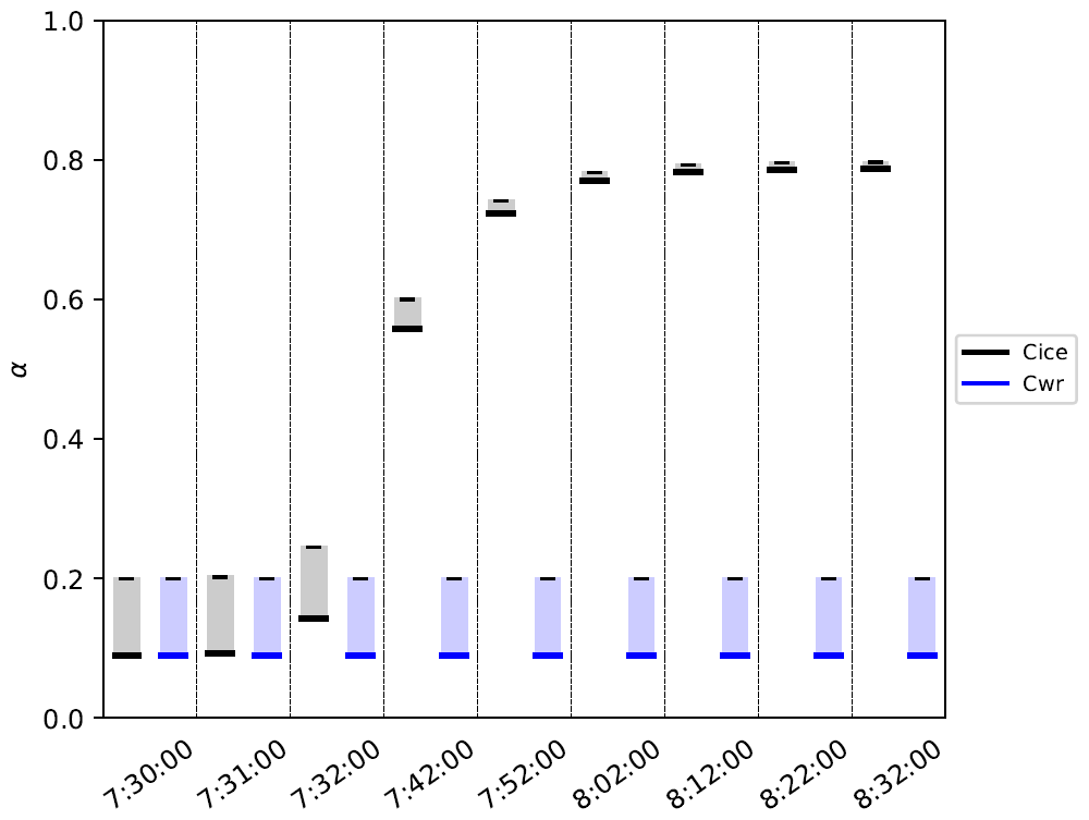
Figure 13 Box plots of albedo α for Cice (dark blue) and Cwr (light blue) show the median and the quartiles. The lower thick line denotes the median while the box represents the quartiles.

6.4.4 Influence of temperature on precipitation

The cloud microphysics parameterisation in MITRAS v3.1, which does not include snow (Cwr, Wwr, Hwr), as well as the one-category ice scheme applied in MITRAS v3.3 (Cice, Wice, Hice) are mass conserving. Therefore, the precipitation amounts on ground are expected to be similar after one hour of simulation, as they depend only on the temperature and not on the used model version (Table 3, hit rate for P 100 % for compared cases Cice and Cwr). For the other meteorological variables, more disagreement with hit rates below 95 % is expected due to the strictness of the required accuracy. Especially for radiation and temperature profound differences are found (Table 3, hit rates below 5 %). The wind field retains some common features (hit rates up to 39 %). In Fig. 14, the spatial mean precipitation amounts on ground over time are presented for rain (dashed lines), snow (dotted lines), and rain + snow (solid lines). As there is no snow in MITRAS v3.1 (Cwr, Wwr, Hwr), the complete precipitation amount is given in dashed lines for these cases, as it equals the rain amount. After half an hour of simulations, the precipitation curves have converged. However, the hit rates of the precipitation amount for the comparisons of MITRAS v3.3 and v3.1 for “hot” (288 K at surface, Hice and Hwr) and warm (280 K at surface, Wice and Wwr) are below 95 % (Table 3), meaning, the results do not lie within the required accuracy. When allowing less strict required accuracies based on observational uncertainties following WMO (2023) (W = 0.1 mm, D = 5 %), the comparison of precipitation of the different model versions yield hit rates of 100 %. This further underlines the sensitivity of the hit rate to the choice of allowed deviation.

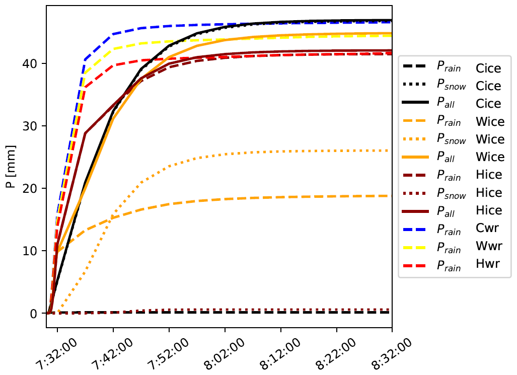
Figure 14 Precipitation amounts on ground for Cice (black), Wice (orange), Hice (brown), Cwr (blue), Wwr (yellow), and Hwr (red). Rain is given in dashed lines, snow in dotted lines and rain and snow together are given as solid lines.

The higher the temperature, the more water vapour the atmosphere can carry before saturation is reached resulting in less precipitation amounts. This is well represented in the model (MITRAS v3.1 and MITRAS v3.3). The final precipitation amounts are smaller for higher temperatures (from black and blue lines over yellow to red curves in Fig. 14). More of rain and snow water content evaporates or sublimates in the sub-saturated areas below the cloud than it would in colder cases. Simultaneously, the production of cloud water content by condensation is reduced. In this study, water vapour is prescribed using the relative humidity leading to temperature dependent specific humidity profiles (Fig. 7). This does not represent that more precipitation is expected in a warming climate (e.g. Purr et al., 2021). For winter in Hamburg, a precipitation amount of over 40 mm after one hour is an extreme case, as synoptic conditions are more favourable for extreme precipitation events in summer than in winter (Weder et al., 2017). As parts of the model extension are also intended to be applied for studies on the impact of heavy precipitation, this extreme case was chosen for the plausibility tests.

6.4.5 Influence of one-category ice scheme

The level of detail is increased in MITRAS v3.3 by extending the model with a one-category ice scheme (Sect. 5) improving the representation of precipitation in winter. During the first minutes of the simulation, the amount of precipitation on ground increases faster with time if only warm precipitation is considered (MITRAS v3.1, dashed lines in Fig. 14) than when also considering the ice phase (MITRAS v3.3, solid lines). In the warm rain Kessler-scheme, the sedimentation of small rain drops is overestimated leading to the calculation of too much precipitation during the process of rain formation (Schlünzen et al., 2018a). This effect is reduced with the one-category ice scheme parameterisation, because precipitation develops slower with this new parameterisation. These changes have consequences on radiation, temperature and wind field, which explains the low hit rates (Table 3).

7 Summary and Conclusions

The microscale and obstacle-resolving model MITRAS was extended by modifying the diffusion of scalars (Sect. 3.1) as well as including boundary conditions for cloud and rain water content at obstacle surfaces (Sect. 3.2) and a snow cover scheme (Sect. 4). The cloud microphysics scheme for warm clouds was extended with a one-category ice scheme (Sect. 5). This makes MITRAS the first obstacle-resolving atmospheric model that includes precipitating snow.

Previous model versions of MITRAS are confirmed to represent well the main features of an urban boundary layer (Schlünzen et al., 2003; Grawe et al., 2013, 2015; Fischereit, 2018). The performance of the warm rain scheme and the newly introduced boundary conditions (v3.1) has been validated by Ferner et al. (2023). The parameterisations for snow cover and the one-category ice scheme have already been applied in mesoscale models (Boettcher, 2017; Doms et al., 2011). The modifications of the parameterisations for the characteristics of a microscale and obstacle-resolving model are validated here by testing for plausibility (Sect. 6) by comparing model results of different model versions (v3.0, v3.1, v3.3). The model features presented in this paper are included in MITRAS v4.0 as are features not relevant to this study (e.g. v3.2, Badeke et al., 2021).

For the plausibility tests, simulations were compared based on a procedure described in VDI (2017) for obstacle-resolving models, where hit rates are calculated for the wind speed components. In our study, additional hit rates for temperature, radiation, and precipitation were determined on the basis of computational accuracy. The resulting required deviations are 0.05 K (0.02 %) for temperature, 0.5 W m⁻² (0.5 %) for long wave radiation, 0.5 W m⁻² (0.2 %) for short wave radiation, and 0.001 mm (1 %) for precipitation.

Comparisons of different model versions reveal that the model produces plausible results. Neglecting terrain-steepness in the diffusion calculation for scalars in MITRAS v3.1 and extending the cloud microphysics scheme in MITRAS v3.3 causes expected differences. The plausibility tests also reveal that taking precipitation into account in a microscale obstacle-resolving model is crucial due to the profound influence of clouds on radiation. Even though state-of-the-art bulk cloud microphysics parameterisations are more complex than the one-category ice scheme applied in MITRAS (Khain et al., 2015), an improvement compared to the previously applied warm rain scheme (Köhler, 1990) has been shown. The overestimation of precipitation during the process of rain formation (Schlünzen et al., 2018a) is reduced.

The homogenising effect of snow on the albedo is plausibly reproduced. In order to increase the level of detail of MITRAS' winter parameterisation, the effects of snow on the roof's albedo or roughness length should be considered. Moreover, the effects of different isolation properties of buildings should be included for instance to study anthropogenic heat emissions on warming and snow melting as well as on the indoor building temperature. For the analyses of frost heterogeneities e.g. on roads and walkways, the inclusion of freezing rain or refreezing snow would be useful, even though it is already possible to derive possible locations of frost from results of the extended model. Refining the crude representation of winter services would lead to further improvements.

The extended model provides the opportunity to perform more realistic simulations of a winter event, where precipitation and obstacles are explicitly resolved. The effects of snow cover and precipitation especially on radiation are better represented. The extended model allows first estimates on influence of different city characteristics on snow heterogeneities. In the future, this information can be used for analyses on frost heterogeneities or human comfort. A sensitivity study extended for an urban neighbourhood is a next step to investigate, how obstacles influence the falling of snow and urban temperature development.

Appendix A: List of symbols

At	parameter for the rain droplet spectrum [${\left({\text{kg\hspace{0.17em}m}}^{-\mathrm{3}}{\text{kg\hspace{0.17em}kg}}^{-\mathrm{1}}\right)}^{\mathrm{0.5}}\text{s}$]
amc	parameter for am(T) (0.08 kg m−2)
amv	parameter for am(T) (0.02 kg m−2)
am(T)	mass-size relation of snow [kg m−2]
$B_{\text{acc}}^{\text{c}}$	accretion rate (ice scheme) [${\text{kg\hspace{0.17em}kg}}^{-\mathrm{1}}{\text{s}}^{-\mathrm{1}}$]
$B_{\text{acc}}^{\text{w}}$	accretion rate (warm rain scheme) [${\text{kg\hspace{0.17em}kg}}^{-\mathrm{1}}{\text{s}}^{-\mathrm{1}}$]
$B_{\text{au}}^{\text{c}}$	autoconversion rate (ice scheme) [${\text{kg\hspace{0.17em}kg}}^{-\mathrm{1}}{\text{s}}^{-\mathrm{1}}$]
$B_{\text{au}}^{\text{w}}$	autoconversion rate (warm rain scheme) [${\text{kg\hspace{0.17em}kg}}^{-\mathrm{1}}{\text{s}}^{-\mathrm{1}}$]
Bcfrz	contact nucleation rate [${\text{kg\hspace{0.17em}kg}}^{-\mathrm{1}}{\text{s}}^{-\mathrm{1}}$]
Bcond	condensation rate [1]
Bdep	deposition rate [${\text{kg\hspace{0.17em}kg}}^{-\mathrm{1}}{\text{s}}^{-\mathrm{1}}$]
Bevap	evaporation rate [${\text{kg\hspace{0.17em}kg}}^{-\mathrm{1}}{\text{s}}^{-\mathrm{1}}$]
bh	roof height [m]
Bifrz	immersion freezing rate [${\text{kg\hspace{0.17em}kg}}^{-\mathrm{1}}{\text{s}}^{-\mathrm{1}}$]
Bmelt	melting rate [${\text{kg\hspace{0.17em}kg}}^{-\mathrm{1}}{\text{s}}^{-\mathrm{1}}$]
Bnuc	nucleation rate [${\text{kg\hspace{0.17em}kg}}^{-\mathrm{1}}{\text{s}}^{-\mathrm{1}}$]
Brim	riming rate [${\text{kg\hspace{0.17em}kg}}^{-\mathrm{1}}{\text{s}}^{-\mathrm{1}}$]
Bshe	shedding rate [${\text{kg\hspace{0.17em}kg}}^{-\mathrm{1}}{\text{s}}^{-\mathrm{1}}$]
B*	heat conduction parameter [${\text{m}}^{\mathrm{2}}\text{K}{\text{W}}^{-\mathrm{1}}{\text{s}}^{-\mathrm{1}}$]
cp	specific heat capacity of dry air at constant pressure [${\text{J\hspace{0.17em}kg}}^{-\mathrm{1}}{\text{K}}^{-\mathrm{1}}$]
cice	specific heat capacity of ice [${\text{Jkg}}^{-\mathrm{1}}{\text{K}}^{-\mathrm{1}}$]
cv,snow	volumetric heat capacity of snow [${\text{JK}}^{-\mathrm{1}}{\text{m}}^{-\mathrm{3}}$]
D	threshold value for relative deviation [1]
DVDI	threshold value for relative deviation for wind speed following VDI (2017) (0.05)
E	rate of evaporation on ground [m s−1]
Ecf	collection efficiency ($\mathrm{5.0}\times {\mathrm{10}}^{-\mathrm{3}}$)
F	correction factor [1]
Fv	ventilation factor [1]
${\stackrel{\mathrm{‾}}{F}}_{\stackrel{\mathrm{‾}}{\mathit{\varphi }}}$	diffusion term
${\stackrel{\mathrm{‾}}{F}}_{\stackrel{\mathrm{‾}}{\mathit{\varphi }},{\dot{x}}^{\mathrm{1}}}$	diffusion term in x-direction
Gsoil	heat flux to soil [W m−2]
h	orography height [m]
HS	sensible heat flux [W m−2]
hsnow	depth of daily temperature wave in snow [m]
hsoil	depth of daily temperature wave in soil [m]
i	location index [1]
Khor	horizontal exchange coefficient [m2s−1]
Kver	vertical exchange coefficient [m2s−1]
$k_{\text{cold}}^{\text{s}}$	inverse autoconversion interval for snow (${\mathrm{10}}^{-\mathrm{3}}{\text{s}}^{-\mathrm{1}}$)
$k_{\text{cold}}^{\text{r}}$	inverse autoconversion interval for rain in ice scheme (${\mathrm{10}}^{-\mathrm{4}}{\text{s}}^{-\mathrm{1}}$)
ksnow	thermal diffusivity in snow [m2 s−1]
ksoil	thermal diffusivity in soil [m2 s−1]
$k_{\text{warm}}^{\text{r}}$	inverse autoconversion interval for rain in warm rain scheme (${\mathrm{10}}^{-\mathrm{3}}{\text{s}}^{-\mathrm{1}}$)
L21	latent heat of vapourisation [J kg−1]
L31	latent heat of sublimation [J kg−1]
L32	latent heat of fusion [J kg−1]
LWnet	net surface long wave radiation [W m−2]
LS	latent heat flux [W m−2]
Msnow	melting rate of SWE on ground [m s−1]
N	total number of compared values [1]
Ncf,0	concentration of natural contact ice nuclei active at −4 °C at sea level (2.0×105)
ni	hit/fail [1]
O	observation/older model version
P	precipitation amount on ground
Pd	prediction/newer model version
p0	basic state atmospheric pressure [Pa]
pref	reference pressure (100 000 Pa)

pS	atmospheric pressure on ground surface [Pa]
$p_{{\text{snow}}_{{\text{z}}_{\mathrm{0}}}}$	snow cover fraction [1]
Prsnow	rate of snowfall [m s−1]
q	hit rate [%]
$q_{\mathrm{1}}^{\mathrm{1}}$	specific humidity [kg kg−1]
$q_{\mathrm{1},\text{sat}}^{\mathrm{1}}$	saturation specific humidity over water [kg kg−1]
$q_{\mathrm{1},\text{sat},\text{ice}}^{\mathrm{1}}$	saturation specific humidity over ice [kg kg−1]
$q_{\mathrm{1}}^{\mathrm{2}\text{c}}$	cloud water content [kg kg−1]
$q_{\mathrm{1},\text{cri}}^{\mathrm{2}\text{c}}$	critical value for autoconversion (${\mathrm{10}}^{-\mathrm{3}}{\text{kg\hspace{0.17em}kg}}^{-\mathrm{1}}$)
$q_{\mathrm{1}}^{\mathrm{2}\text{r}}$	rain water content [kg kg−1]
$q_{\mathrm{1}}^{\mathrm{3}\text{s}}$	snow water content [kg kg−1]
R	gas constant for dry air [${\text{Jkg}}^{-\mathrm{1}}{\text{K}}^{-\mathrm{1}}$]
S	saturation [%]
SWE	snow water equivalent [m]
SWEcrit	critical SWE (0.05 m)
SWnet	net surface short wave radiation [W m−2]
T	temperature [K]
T0	freezing point (273.16 K)
T1	minimum temperature for mass-size relation of snow (253.16 K)
T2	minimum temperature for temperature function (235.16 K)
Th,soil	deep soil temperature [K]
TS	temperature on ground surface [K]
t	time [s]
u	wind in west-east direction [m s−1]
Uref	reference wind speed [m s−1]
v	wind in south-north direction [m s−1]
vTR	terminal velocity of rain [m s−1]
vTS	terminal velocity of snow [m s−1]
W	threshold value for absolute deviation
WVDI	threshold value for absolute deviation for wind speed following VDI (2017) (0.01 m s−1)
w	wind in vertical direction [m s−1]
x	horizontal coordinate in west-east direction in Cartesian coordinate system [m]
${\dot{x}}^{\mathrm{1}}$	coordinate in terrain-following coordinate system [m]
${\dot{x}}^{\mathrm{2}}$	coordinate in terrain-following coordinate system [m]
${\dot{x}}^{\mathrm{3}}$	coordinate in terrain-following coordinate system [m]
y	horizontal coordinate in south-north direction in Cartesian coordinate system [m]
z	vertical coordinate in Cartesian coordinate system [m]
z0	roughness length [m]
$z_{{\mathrm{0}}_{\text{ini}}}$	initial z0 without snow cover [m]
$z_{{\mathrm{0}}_{\text{snow}}}$	snow roughness length (10−3 m)
zsnow	snow depth [m]
α	albedo [1]
αcf	contact nucleation factor ($\mathrm{1.55}\times {\mathrm{10}}^{-\mathrm{3}}$)
αcond	condensation parameter [1]
αdep	deposition factor [1]
αif	immersion freezing factor ($\mathrm{9.95}\times {\mathrm{10}}^{-\mathrm{5}}$)
αini	initial α without snow cover [1]
αmax	maximum αsnow (0.85)
αmelt	melting factor ($\mathrm{7.2}\times {\mathrm{10}}^{-\mathrm{6}}$)
αmin	minimum αsnow (0.18)
αmin,J14	minimum αsnow following Järvi et al. (2014) (0.18)

αmin,V91	minimum αsnow following Verseghy (1991) (0.5)
α*	grid volume [m3]
β	empirical factor for roughness length (0.408)
βdep	deposition factor (13.0)
βmelt	melting factor (13.0)
ΔSWE	difference of SWE [m]
ΔSWnet	difference of SWnet [W m−2]
Δt	time step [s]
Δv	difference of v wind component [m s−1]
ϵ	very small number (10−6)
ϵ(T)	temperature function [1]
θ	potential temperature [K]
νice	thermal conductivity of ice [${\text{W\hspace{0.17em}m}}^{-\mathrm{1}}{\text{K}}^{-\mathrm{1}}$]
νsnow	thermal conductivity of snow [${\text{W\hspace{0.17em}m}}^{-\mathrm{1}}{\text{K}}^{-\mathrm{1}}$]
νsoil	thermal conductivity of soil [${\text{W\hspace{0.17em}m}}^{-\mathrm{1}}{\text{K}}^{-\mathrm{1}}$]
ρ0	basic state atmospheric density [kg m−3]
ρice	density of ice (918.9 kg m−3)
ρmax	maximum ρsnow (300 kg m−3)
ρmin	minimum ρsnow (100 kg m−3)
ρref	reference density (1.29 kg m−3)
ρsnow	snow pack density [kg m−3]
ρw	density of water [kg m−3]
τ	period of temperature wave (86400 s)
τ1	time period parameter (86400 s)
τf	empirical parameter for ρsnow (0.24)
τf,α	empirical parameter for albedo (0.11)
${\mathit{\tau }}_{\text{f},\mathit{\alpha },\text{J14}}$	empirical parameter for albedo following Järvi et al. (2014) (0.11)
${\mathit{\tau }}_{\text{f},\mathit{\alpha },\text{V91}}$	empirical parameter for albedo following Verseghy (1991) (0.24)
τα	empirical parameter for albedo (0.18)
τα,J14	empirical parameter for albedo following Järvi et al. (2014) (0.18)
τα,V91	empirical parameter for albedo following Verseghy (1991) (0.008)
ϕ	any scalar quantity
ϕ0	basic state part of ϕ
$\stackrel{\mathrm{̃}}{\mathit{\varphi }}$,	deviation of ϕ