Effect of inlet turbulence on the large eddy simulation of fire plume turbulent characteristics near the ground

Fire hazard has become a severe threat for ecosystem and urban city. Accurate modelling of fire behaviour and pollutant transport in the atmospheric boundary layer is important for fire risk management. The effect of using turbulent inflow model on simulating fire plume development remains unclear. To understand whether it is important or not for large eddy simulations of fire plume, we performed numerical experiments of fire combustions under uniform and turbulent inflows, and considered two wind velocities, representing weak and moderate conditions respectively. Results show that the assumption of uniform flow does not have significant effect on the mean temperature and velocity fields for weak wind but obvious effect for moderate wind. Turbulent fluctuations of the fire flame indicates that fire plume development modelling is more influenced by the background wind turbulence under relatively larger velocity.

1 Introduction

Fire hazard has become a severe issue in recent years and post significant threat for ecosystem and urban city (Liu et al., 2021). Accurate modelling of fire behaviour and pollutant transport in the atmospheric boundary layer is important for fire risk management (Gajendiran et al., 2024; Song et al., 2022). Due to strong heat released by the fire, the fire plume updraft is dominated by the buoyant force under quiet atmosphere (Maragkos and Merci, 2020). Under windy atmosphere, the fire development is influenced by the combined effect of wind inertial and flame buoyance (Pimont et al., 2012). For the large eddy simulation of atmospheric boundary layer (ABL), turbulence must be accurately modelled (Stoll et al., 2020).

Modelling strategy of turbulence for applications related to ABL are extensively investigated. An important component of this modelling is the turbulent inflow condition (Yang et al., 2020). The simplest method is to neglect the velocity fluctuation for the inflow and assumes a uniform velocity profile, which has non-negligible effect on the wind-building interaction modelling (Cheng et al., 2025). Advanced turbulent generation methods have been proposed for the inflow boundary condition, such as the precursor-successor method and the synthetic method. The precursor method is accurate and simple to use but needs more computation load (more time for precursor run and more space requirement for inlet data storage), and the synthetic methods are less computational expensive. There are different kinds of synthetic methods available in literatures (Melaku and Bitsuamlak, 2021). These inflow generation methods are frequently used for building (Melaku and Bitsuamlak, 2024) and turbine simulations (Stanislawski et al., 2023). Recently, this kind of inflow turbulence generation model has also been implemented in WRF (Weather Research and Forecasting) for large eddy simulations (Zhong et al., 2021).

Modelling the inflow turbulence is found to have significant effect on the downstream pollutant transport and wake flow (Yang and Sotiropoulos, 2019). However, in the modelling of fire plume development, the turbulent inflow condition receives much less attention, although these exist several studies considering turbulent approaching flow. In general, fire releases a large amount of heat in a short time, the turbulent flow near the flame is dominated by the buoyant flow and its associated entrainment flow (Ahmed and Trouvé, 2021; Sun et al., 2022). The oscillation of the flame is also mainly controlled by the puffing frequency of the fire plume, which is much less than that of the background wind turbulence. Many studies used a uniform velocity without turbulence or a simplified turbulent method for the approaching flow, which does not represent the true turbulent condition. Eftekharian et al. (Eftekharian et al., 2019, 2020) performed large eddy simulations of wind and fire interactions for different configurations, and used the “2D vortex method” to induce turbulent fluctuations, which was realized by the “turbulentInlet” boundary condition available in OpenFOAM (Open Field Operation And Manipulation) libraries. Edalati-nejad et al. (Edalati-Nejad et al., 2021) also used the random noise method to generate velocity fluctuations for simulations of fires on a sloped terrain. However, they did not discuss the role of this turbulent inflow on the fire heat and flow characteristics. Sun et al. (Sun et al., 2024a, b) used the uniform inflow method for their investigations of fire plume interactions with an idealized building and two-dimensional ridge. This simplified uniform inflow condition may cause errors for pressure coefficient predictions on a building, but how it affects the fire plume interactions with building or ridge were not discovered. Several studies adopted turbulent inflow for their fire modelling (Ding et al., 2025; Ong et al., 2022; Wang et al., 2023) with the precursor method or the synthetic method, but its roles in the fire plume development were not investigated.

From above review, the effect of using turbulent inflow model on simulating fire plume development has not been clearly established, and there is no consensus about its significance. To determine whether it is important for fire plume simulation near the ground, we performed large eddy simulations of fire combustions under uniform and turbulent inflows for two wind velocities, representing weak and moderate wind respectively. Section 2 presents the numerical methods and boundary conditions for the fire combustion modelling and Sect. 3 provides detailed comparisons of mean temperature and velocity fields and turbulent statistics under different conditions, followed by conclusions and discussions.

2 Methods

2.1 Mathematic formulations and physical models

The fire flame is simulated by a turbulent diffusion combustion model, which considers mass transfer, momentum transfer, species transfer, and energy transfer:

$$\begin{array}{}\text{(1)}& {\displaystyle }& {\displaystyle }{\displaystyle \frac{\partial \stackrel{\mathrm{‾}}{\mathit{\rho }}}{\partial t}}+{\displaystyle \frac{\partial \stackrel{\mathrm{‾}}{\mathit{\rho }}{\stackrel{\mathrm{̃}}{u}}_i}{\partial x_i}}=\mathrm{0},\text{(2)}& {\displaystyle }& {\displaystyle }{\displaystyle \frac{\partial \stackrel{\mathrm{‾}}{\mathit{\rho }}{\stackrel{\mathrm{̃}}{u}}_j}{\partial t}}+{\displaystyle \frac{\partial \stackrel{\mathrm{‾}}{\mathit{\rho }}{\stackrel{\mathrm{̃}}{u}}_i{\stackrel{\mathrm{̃}}{u}}_j}{\partial x_i}}=-{\displaystyle \frac{\partial \stackrel{\mathrm{‾}}{p}}{\partial x_j}}+{\displaystyle \frac{\partial }{\partial x_i}}\left((\stackrel{\mathrm{̃}}{\mathit{\mu }}+{\mathit{\mu }}_{\mathrm{t}}){\stackrel{\mathrm{̃}}{S}}_{ij}\right)+\stackrel{\mathrm{‾}}{\mathit{\rho }}g,\end{array}$$

$$\begin{array}{}\text{(3)}& {\displaystyle }& {\displaystyle }{\displaystyle \frac{\partial \stackrel{\mathrm{‾}}{\mathit{\rho }}{\stackrel{\mathrm{̃}}{Y}}_k}{\partial t}}+{\displaystyle \frac{\partial \stackrel{\mathrm{‾}}{\mathit{\rho }}{\stackrel{\mathrm{̃}}{u}}_i{\stackrel{\mathrm{̃}}{Y}}_k}{\partial x_i}}={\displaystyle \frac{\partial }{\partial x_i}}\left(\stackrel{\mathrm{‾}}{\mathit{\rho }}\left(D_k+{\displaystyle \frac{{\mathit{\nu }}_{\text{sgs}}}{S{c}_{\mathrm{t}}}}\right){\displaystyle \frac{\partial {\stackrel{\mathrm{̃}}{Y}}_k}{\partial x_i}}\right)+\stackrel{\mathrm{‾}}{{\dot{\mathit{\omega }}}_k^{\prime \prime \prime }},\text{(4)}& {\displaystyle }& {\displaystyle }{\displaystyle \frac{\partial \stackrel{\mathrm{‾}}{\mathit{\rho }}\stackrel{\mathrm{̃}}{h}}{\partial t}}+{\displaystyle \frac{\partial \stackrel{\mathrm{‾}}{\mathit{\rho }}{\stackrel{\mathrm{̃}}{u}}_i\stackrel{\mathrm{̃}}{h}}{\partial x_i}}={\displaystyle \frac{\partial }{\partial x_i}}\left(\stackrel{\mathrm{‾}}{\mathit{\rho }}\left(D_{\text{th}}+{\displaystyle \frac{{\mathit{\nu }}_{\text{sgs}}}{{\text{Pr}}_{\mathrm{t}}}}\right){\displaystyle \frac{\partial \stackrel{\mathrm{̃}}{h}}{\partial x_i}}\right)+\stackrel{\mathrm{‾}}{{\dot{q}}_c},\end{array}$$

where overbars denote density-based variables and tildes denote Favre-based variables. $\stackrel{\mathrm{‾}}{\mathit{\rho }}$ is the density, $\stackrel{\mathrm{̃}}{u}$ is the velocity, $\stackrel{\mathrm{‾}}{p}$ is the pressure, $\stackrel{\mathrm{̃}}{\mathit{\mu }}$ is the dynamic viscosity, μ_t is the turbulent viscosity, ${\stackrel{\mathrm{̃}}{S}}_{ij}$ is the shear stress, g is the gravitational force, ${\stackrel{\mathrm{̃}}{Y}}_k$ is the mass fraction of species k, D_k is the mass diffusion coefficient, Sc_t is the turbulent Schmidt number, ν_sgs is the sub-grid scale viscosity, $\stackrel{\mathrm{‾}}{{\dot{\mathit{\omega }}}_k^{\prime \prime \prime }}$ is the chemical reaction rate, $\stackrel{\mathrm{̃}}{h}$ is the enthalpy, D_th is the thermal diffusion coefficient, Pr_t is the turbulent Prandtl number. The Lewis number is assumed to be unity.

The sub-grid scale turbulent kinetic energy k_sgs is modelled by a one-eddy equation:

$$\begin{array}{}\text{(5)}& {\displaystyle \frac{\partial \left(\stackrel{\mathrm{‾}}{\mathit{\rho }}{k}_{\text{sgs}}\right)}{\partial t}}+\mathrm{\nabla }\cdot \left(\stackrel{\mathrm{‾}}{\mathit{\rho }}\stackrel{\mathrm{̃}}{u}{k}_{\text{sgs}}\right)=\mathrm{\nabla }\cdot \left((\mathit{\mu }+{\mathit{\mu }}_{\mathrm{t}})\mathrm{\nabla }{k}_{\text{sgs}}\right)+P-\stackrel{\mathrm{‾}}{\mathit{\rho }}{\mathit{\epsilon }}_{\text{sgs}}\end{array}$$

where μ_t is the turbulent viscosity, and calculated by ${\mathit{\mu }}_{\mathrm{t}}=\stackrel{\mathrm{‾}}{\mathit{\rho }}{c}_k\mathrm{\Delta }\sqrt{k_{\text{sgs}}}$.

The flame fuel is assumed to be methane vapor, which flows into the domain through the fuel inlet surface. The combustion occurs immediately once the methane vapor mixes with air under the assumption of eddy dissipation process, which is a widely used model for diffusion flame. Chemical reaction is modelled by one-step global reaction of methane:

$$\begin{array}{}\text{(R1)}& {\mathrm{CH}}_{\mathrm{4}}+{\mathrm{O}}_{\mathrm{2}}={\mathrm{CO}}_{\mathrm{2}}+\mathrm{2}{\mathrm{H}}_{\mathrm{2}}\mathrm{O}.\end{array}$$

The heat of combustion of the methane is about $\mathrm{5}\times {\mathrm{10}}^{\mathrm{7}}\mathrm{J}{\mathrm{kg}}^{-\mathrm{1}}$, which controls heat release rate of the fuel. Detailed reaction mechanism can be considered for more advanced combustion simulation, but is beyond the purpose of this work. This one-step global reaction is widely used in fire modelling due to its simplicity and efficiency, but it cannot predict complex flame dynamics, such as ignition and extinction process.

Figure 1 shows the physical model considered in this work, and the computational domain sizes are 150 m in length, 80 m in wide and 100 m in height. The fire source (methane vapor inlet) is 40 m away from the Inlet surface, which is the wind inlet. The Outlet surface is the exit for the flow. The top surface is set as slip boundary for the velocity and zero gradient for other variables. A Rayleigh damping layer is adopted at the upper 10 % of the domain to eliminate the oscillating wave caused by density variations. To minimize the effect of top boundary on the flame plume development near the ground, the length and height are chosen to make sure the plume mainly exits the domain through the outlet surface. The back and front surface (not labelled) are set as slip for velocity and zero gradient for other variables. Friction at the bottom surface is modelled by a universal law available in OpenFOAM. The fire source is 2 m wide. To capture temperature and velocity variation near the flame, mesh is refined in this region. The mesh consists of four level grids, as shown in Fig. 2. The first level is adopted for the whole domain, the second level is used between (30, 26, 0) and (70, 54, 32), the third level is used between (34, 34, 0) and (60, 46, 12), and the fourth level is used between (38, 37, 0) and (48, 43, 5). This refined mesh leads to a mesh size of 0.125 m in x direction, 0.125 m in y direction and 0.03 m in z direction. The total number of mesh is about 3.79 million.

Figure 1 Schematic of physical model and boundary conditions.

Figure 2 Schematic of refined mesh near the fire source.

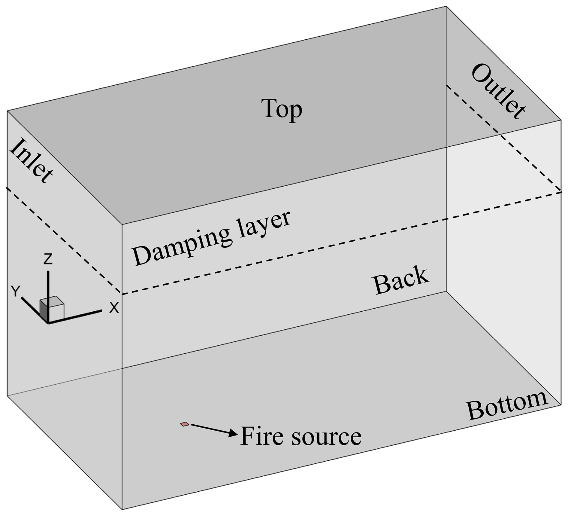
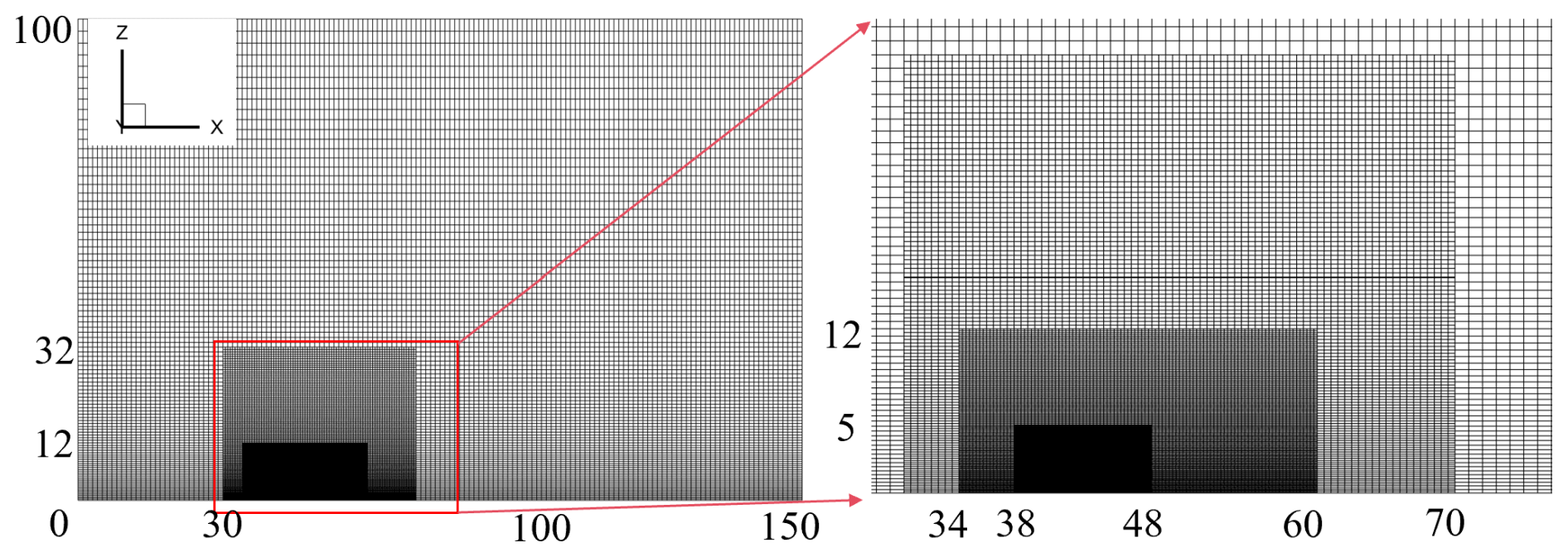
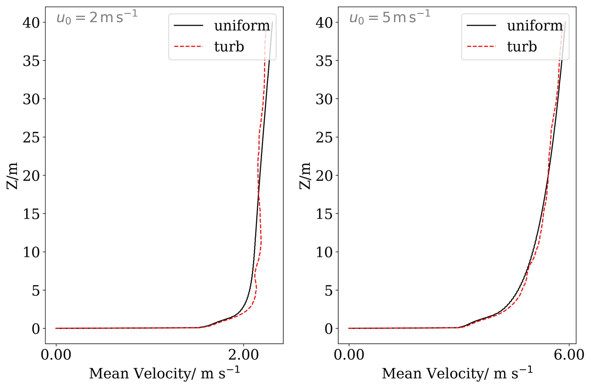
Figure 3 Mean streamwise velocities 2 m before the fire under different conditions. “uniform” means uniform inflow condition, “turb” means turblent inflow condition.

2.2 Numerical schemes

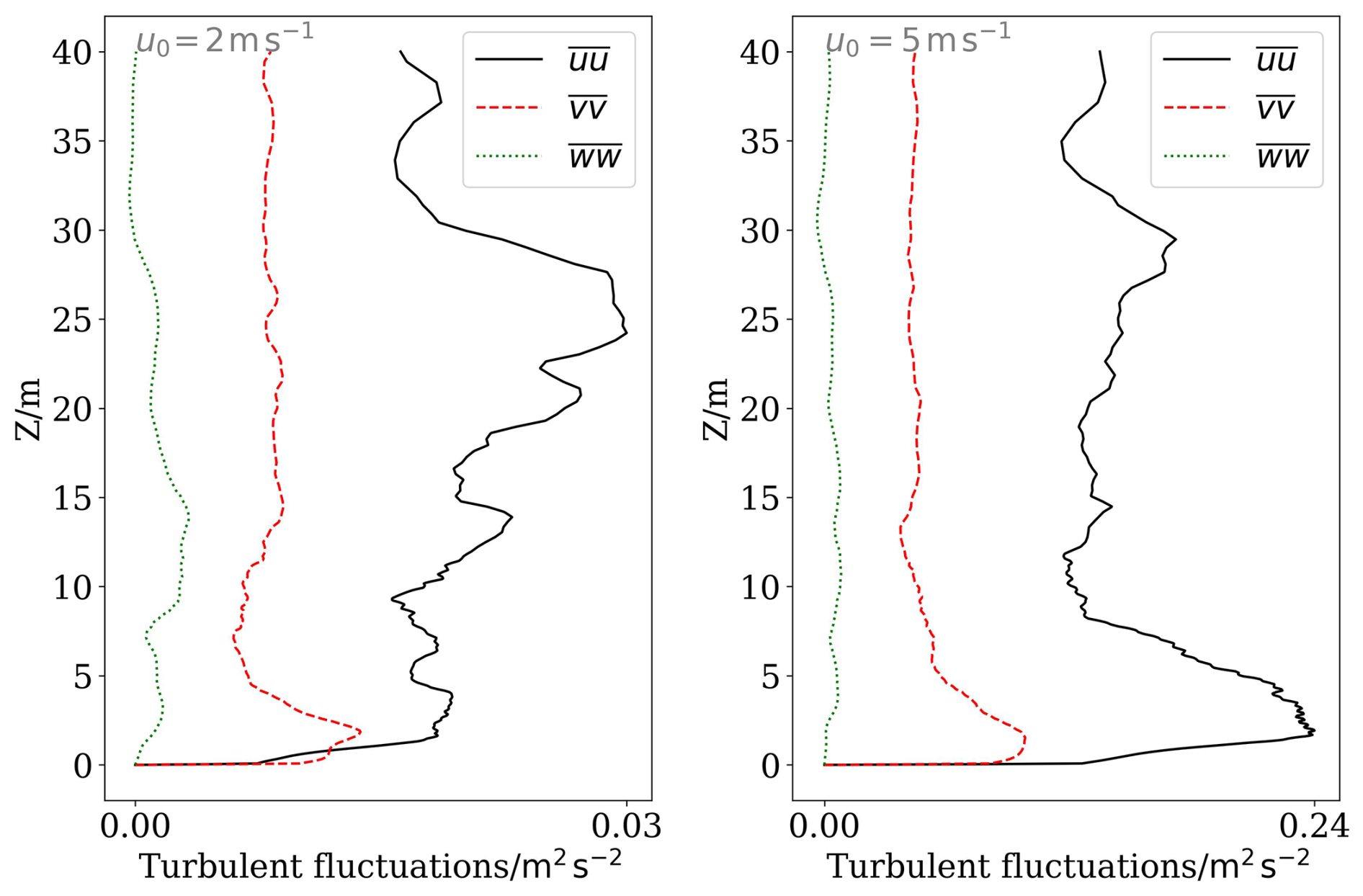
As for the inlet, two kinds of velocity are considered, a uniform fixed velocity and a turbulent velocity. The uniform fixed velocity uses a power-law profile of $U_{\mathrm{0}}\cdot (z/\mathrm{10}{)}^{\mathrm{0.12}}$, and U₀ is the reference velocity, which is set as 2 or 5 m s⁻¹ in the simulations. This uniform velocity does not induce any turbulence at the inlet, and is sometimes used for the fire modelling in the ABL. The turbulent velocity is generated by the divergence-free spectral representation (DFSR) method, whose validity for turbulent ABL has been discussed in its original paper (Melaku and Bitsuamlak, 2021) and is not discussed in this work. Inputs for for this turbulent generation method include mean velocity, turbulent intensities and length scales. The mean velocity profile is same to the uniform case. The turbulent intensities and length scales uses expressions suggested by wind engineering (Yue et al., 2025). In this work, turbulent intensity profile and length scale profile are not varied. We collected the mean velocity profiles and turbulent fluctuations at a location before the fire source. The mean streamwise velocity is shown in Fig. 3 ad velocity fluctuations are shown in Fig. 4. Because averaging time is short (240 s, which is discussed later), these profiles have oscillations. From Fig. 3, the mean velocity of the turbulent condition is close to that of the uniform case, but with small deviations from the mean uniform velocity profile due to turbulence. From Fig. 4, velocity fluctuations of the 2 m s⁻¹ case are less than 0.03 m² s⁻², and are less than 0.24 for the 5 m s⁻¹ case because we used similar turbulent intensities for both cases.

Figure 4 Mean velocities fluctuations 2 m before the fire source under different conditions.

The Euler method is adopted for the time discretization, and the time step is variable with the maximum Courant number smaller than 0.8. A central differencing scheme with flux limiter is used for the momentum convection term, and total variation diminishing scheme with limiter is applied for the energy and species convection terms, and the species are additionally bounded between 0 and 1. The PIMPLE method (PISO and SIMPLE combined) is used for the pressure-velocity coupling with 3 outer correctors and 2 correctors. Pre-conditioned gradient solver is used for the density and the GAMG (geometric-algebraic multi-grid) with Gauss–Seidel smoother is adopted for pressure equation, while Preconditioned Bi-Conjugate Gradient Stabilized (PBiCGStab) solvers are used for the velocity, energy and species equations. The detailed model parameters can be seen in the file (Sun, 2025).

The simulation process is spin-up for the first 200 s without fuel vapor and combustion. After 200 s, the fuel vapor starts to enter the domain through its inlet and burns immediately when encountering air. Time averaging is activated from 250 s to avoid the effect of initial combustion on the statistic. Total averaging time lasts 240 s, which corresponds to about 3 and 8 flow-through time for wind velocities of 2 m s⁻¹, 5 m s⁻¹ respectively. This time window is small for obtaining mean values for the background wind turbulent statistics, but this size is enough for the fire plume turbulent statistics due to its more intermittent flow. Time averaged results for the fire plume are found to be not changing when further increasing time averaging window, which are shown in Fig. A1.

3 Results and discussions

3.1 Mean velocity and temperature fields

Figure 5 compares mean velocity magnitudes for uniform and turbulent cases at the Y=40 m plane (left column) and X=50 m plane (right column) for $U_{\mathrm{0}}=\mathrm{2}\mathrm{m}{\mathrm{s}}^{-\mathrm{1}}$. The velocity distributions at both planes are similar for two cases, but they differ in magnitudes. At the Y middle plane, the maximum velocity occurs near X=43 m or both cases, but the magnitude is slightly higher for uniform case. At the X=50 m plane, velocity is bimodal due to counter-rotating vortex pairs, and the uniform case also predicts larger velocity.

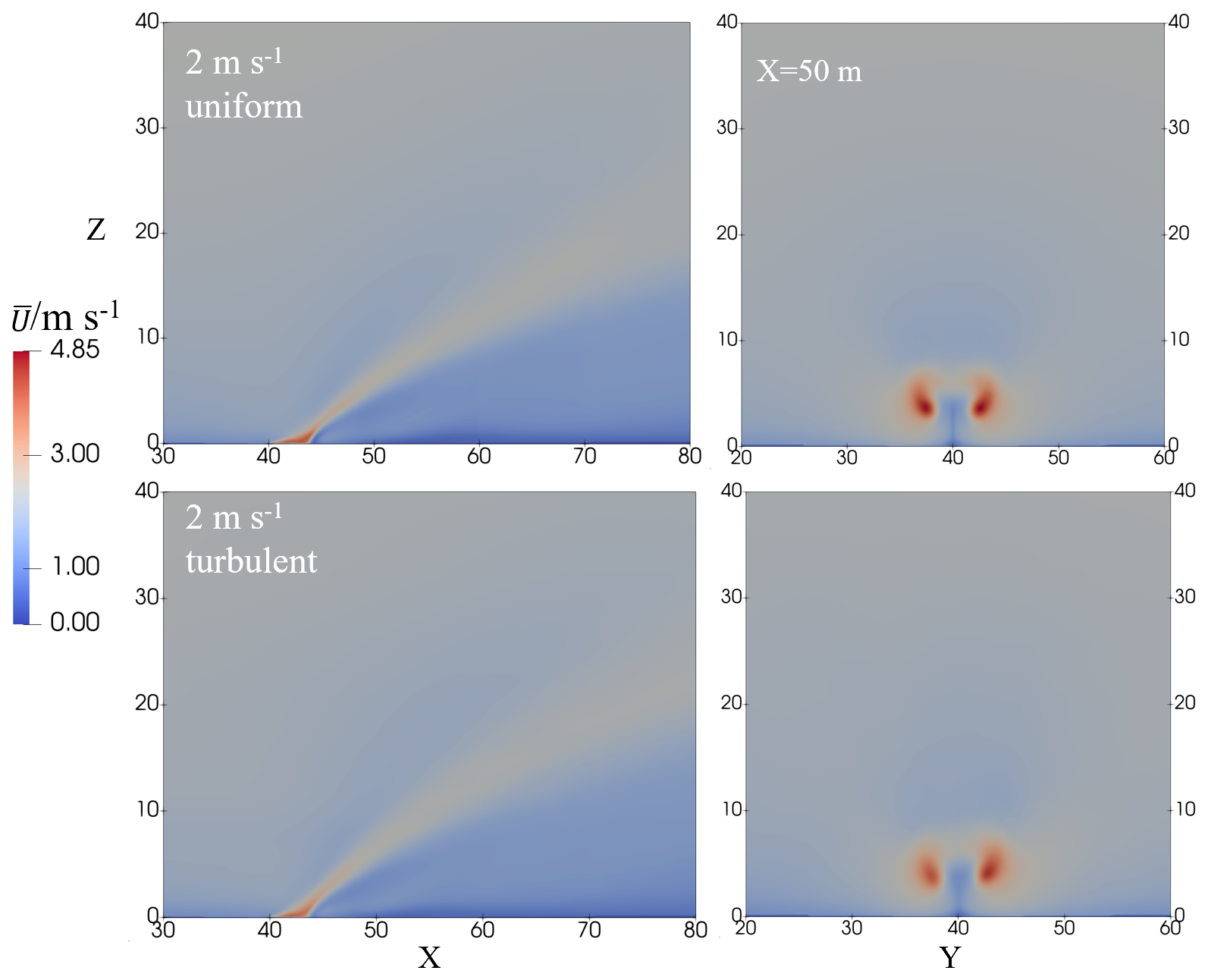
Figure 5 Mean velocity at the Y=40 m plane (left column) and X=50 m plane (right column) for $U_{\mathrm{0}}=\mathrm{2}\mathrm{m}{\mathrm{s}}^{-\mathrm{1}}$. First row for uniform condition, and second row for turbulent condition.

Figure 6 compares mean temperature at the Y=40 m plane (left column) and X=50 m plane (right column) for $U_{\mathrm{0}}=\mathrm{2}\mathrm{m}{\mathrm{s}}^{-\mathrm{1}}$ Temperature distributions are also same for both cases, and the maximum mean temperature can reach about 1650 K. Similar to the velocity fields, temperatures are higher for uniform cases for both the middle Y plane and X plane.

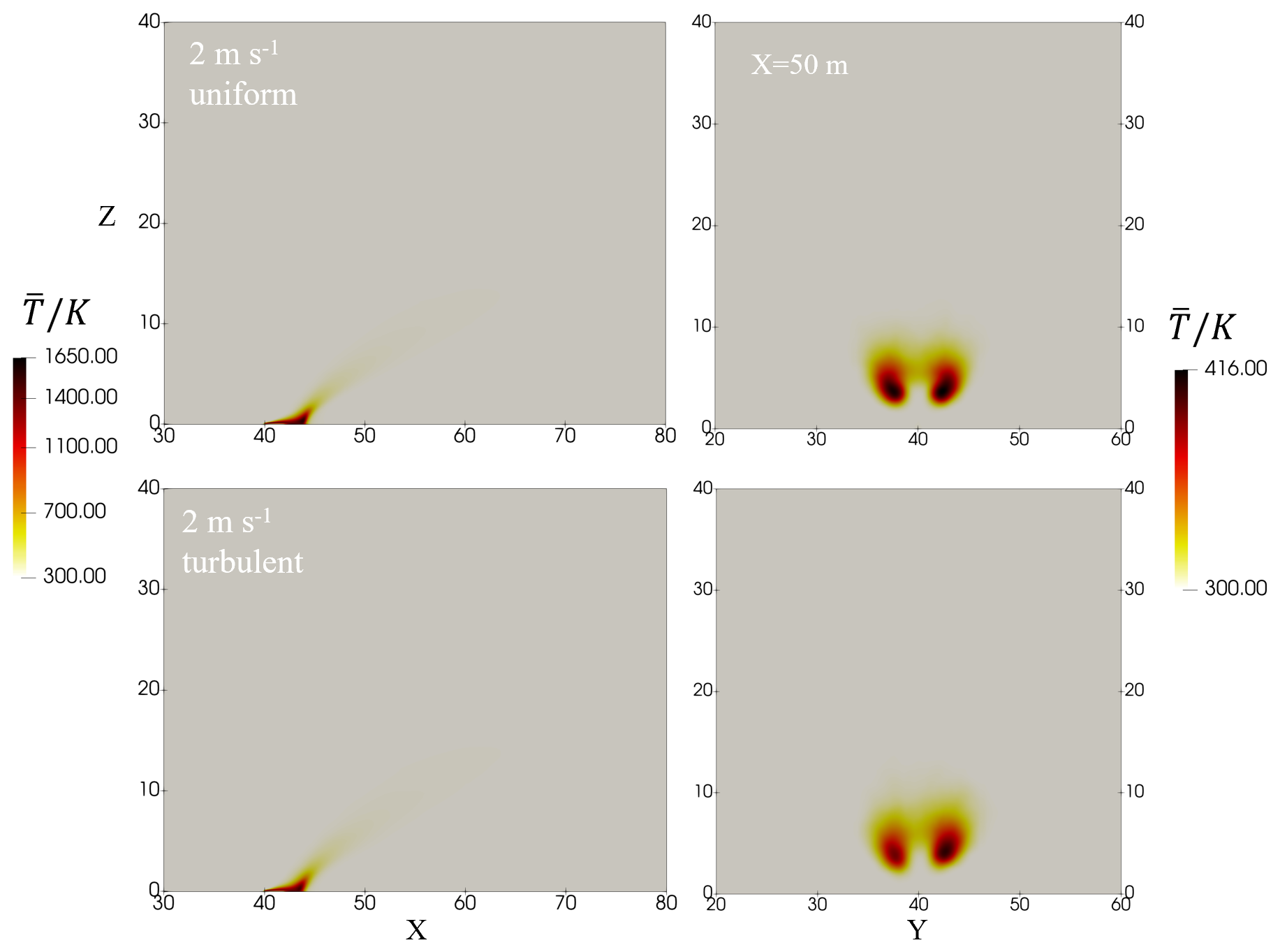
Figure 6 Mean temperature at the Y=40 m plane (left column) and X=50 m plane (right column) for $U_{\mathrm{0}}=\mathrm{2}\mathrm{m}{\mathrm{s}}^{-\mathrm{1}}$. First row for uniform condition, and second row for turbulent condition.

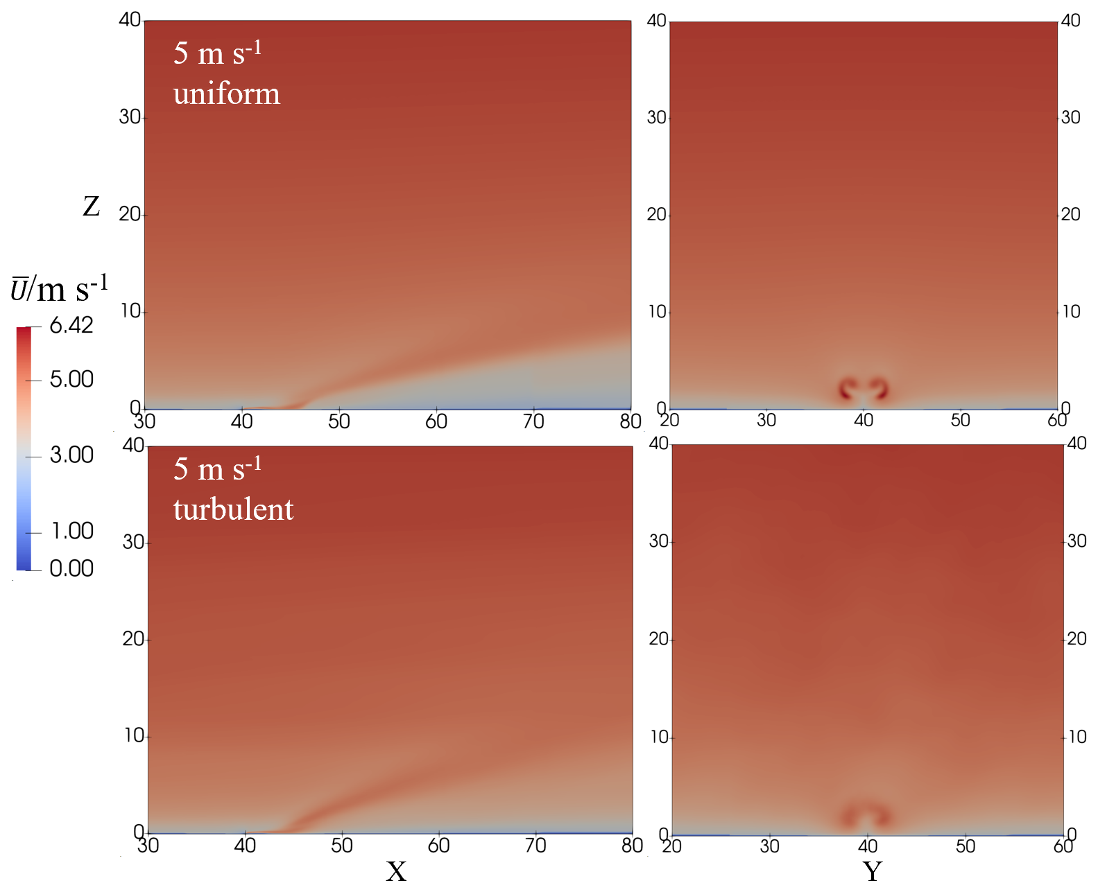
Figure 7 Mean velocity at the Y=40 m plane (left column) and X=50 m plane (right column) for $U_{\mathrm{0}}=\mathrm{5}\mathrm{m}{\mathrm{s}}^{-\mathrm{1}}$. First row for uniform condition, and second row for turbulent condition.

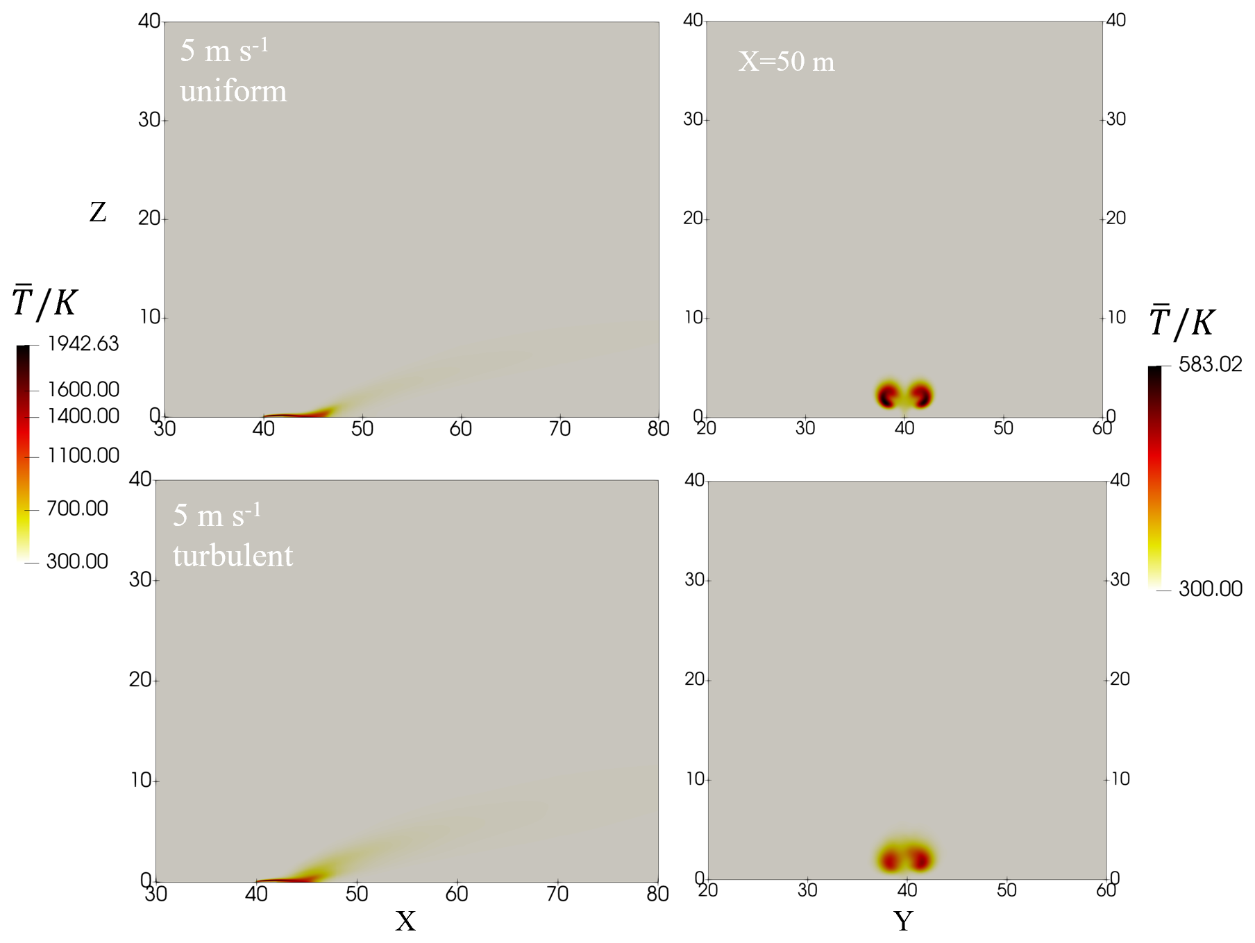
Figure 8 Mean temperature at the Y=40 m plane (left column) and X=50 m plane (right column) for $U_{\mathrm{0}}=\mathrm{5}\mathrm{m}{\mathrm{s}}^{-\mathrm{1}}$. First row for uniform condition, and second row for turbulent condition.

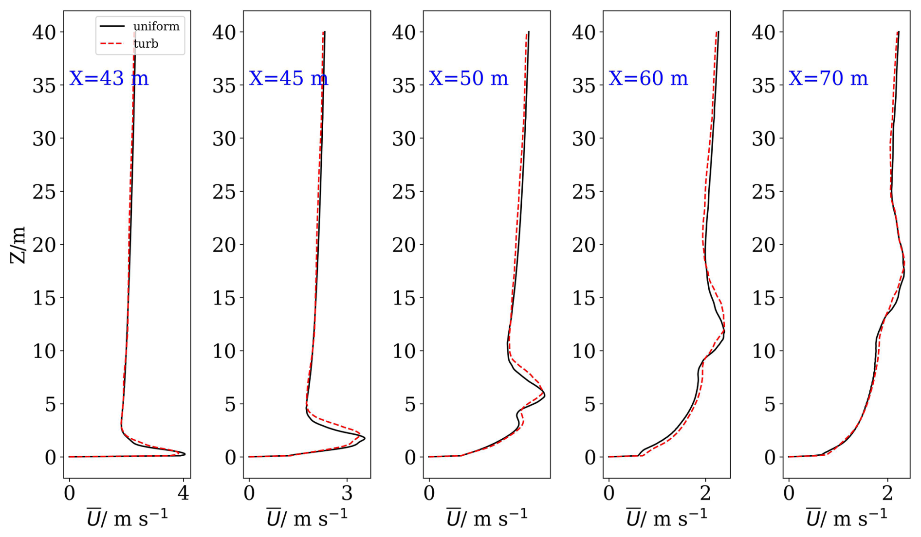
Figure 9 Mean velocity profiles at different X locations for $U_{\mathrm{0}}=\mathrm{2}\mathrm{m}{\mathrm{s}}^{-\mathrm{1}}$. The velocities are extracted from the middle Y plane.

For this weak wind case, the plume inclination is almost the same for the uniform and turbulent case. Temperature is slightly lower and become less symmetric at the X=50 m plane for the turbulent case, and this is maybe caused by strengthened spanwise velocity fluctuations due to turbulence.

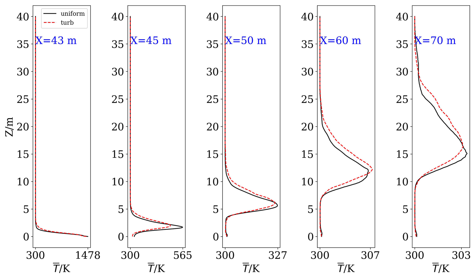
Figure 10 Mean temperature profiles at different X locations for $U_{\mathrm{0}}=\mathrm{2}\mathrm{m}{\mathrm{s}}^{-\mathrm{1}}$. The temperatures are extracted from the middle Y plane.

Figure 7 compares mean velocity magnitudes for uniform and turbulent cases at the Y=40 m lane (left column) and X=50 m lane (right column) for $U_{\mathrm{0}}=\mathrm{5}\mathrm{m}{\mathrm{s}}^{-\mathrm{1}}$. The velocity distributions are similar for two cases at the middle Y plane, but different at the X plane. Due to stronger wind force, plume velocities are much closer to the ground compared to those of 2 m s⁻¹ cases. At the Y middle plane, the maximum velocity induced by the fire heat is much higher for the uniform case. However, for the turbulent case, the velocity is slightly smaller and seems more scattered. At the X=50 m plane, velocity is also higher for the uniform case, with a larger velocity gradient in the core of the plume pairs.

Figure 8 compares mean temperature at the Y=40 m lane (left column) and X=50 m plane (right column) for $U_{\mathrm{0}}=\mathrm{5}\mathrm{m}{\mathrm{s}}^{-\mathrm{1}}$. Temperature distributions are also inclined larger as the velocity fields. The maximum temperature for both cases can reach about 1942 K and occurs at the surface of the fuel vapor. For both cases, the flame cores (temperature larger than 700 K) are almost attached to the ground surface compared to those of the 2 m s⁻¹ case. This is because the wind inertial force is dominant over the buoyant force. Temperature distributions before X=45 m are almost the same for the two cases. At downstream, temperature is more scattered for the turbulent condition. At the X=50 m plane, we can clearly see that the temperature is much higher for the uniform case, with larger values occurring near the bottom of the plume pairs.

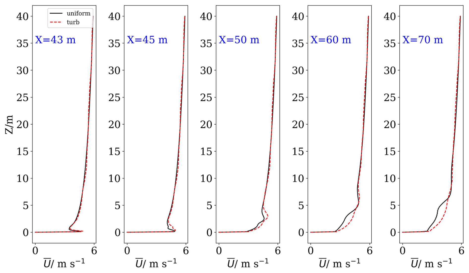
Figure 11 Mean velocity profiles at different x locations for $U_{\mathrm{0}}=\mathrm{5}\mathrm{m}{\mathrm{s}}^{-\mathrm{1}}$. The velocities are extracted from the middle Y plane.

Figures 9 and 10 shows the mean velocity and temperature profiles along height at different X locations for $U_{\mathrm{0}}=\mathrm{2}\mathrm{m}{\mathrm{s}}^{-\mathrm{1}}$. At $X=\mathrm{43}-\mathrm{70}\mathrm{m}$, it can be clearly seen the velocity profiles of two cases are almost identical except that velocity of the turbulent case is slightly higher at some heights at $X=\mathrm{45}-\mathrm{60}$. Maximum velocities of two cases are also close to each other. The dashed red lines seem smoother than the solid black lines, and this means the turbulent inflow does not necessarily lead to more fluctuated flow for this fire plume.

Comparison of temperature profiles shows some differences compared to those of the velocities (Fig. 10). Temperature of the turbulent case is smaller at X=45 m, but larger at X≧50 m. At X>50 m, the mean temperature of turbulent case is larger than that of the uniform case. The differences become gradually smaller at further downwards and the fire plume for the turbulent case is slightly higher

Figure 11 and 12 show the mean velocity and temperature profiles along height at different x locations for $U_{\mathrm{0}}=\mathrm{5}\mathrm{m}{\mathrm{s}}^{-\mathrm{1}}$. Velocity profiles of two cases are very close to each other and almost identical at X=43 m. Compared to the 2 m s⁻¹ condition, a sharp increase of velocity can be observed near the ground surface, which is a consequence of larger inertial under 5 m s⁻¹ condition. At further downstream, the velocity profiles of turbulent case are smoother and larger near the ground surface. Temperature profiles are also close to each other for two cases before X=45 m. Maximum temperatures of turbulent case are larger at downstream, and the maximum difference is located at X=50 m. Temperature profiles of uniform case have narrower gaussian shapes at X≧50 m. This indicates that the uniform inflow method will decrease the vertical transport of momentum and heat flux.

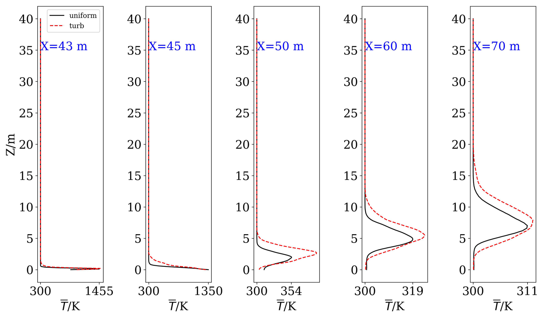
Figure 12 Mean temperature profiles at different x locations for $U_{\mathrm{0}}=\mathrm{5}\mathrm{m}{\mathrm{s}}^{-\mathrm{1}}$. The temperatures are extracted from the middle Y plane.

3.2 Turbulent fluctuations

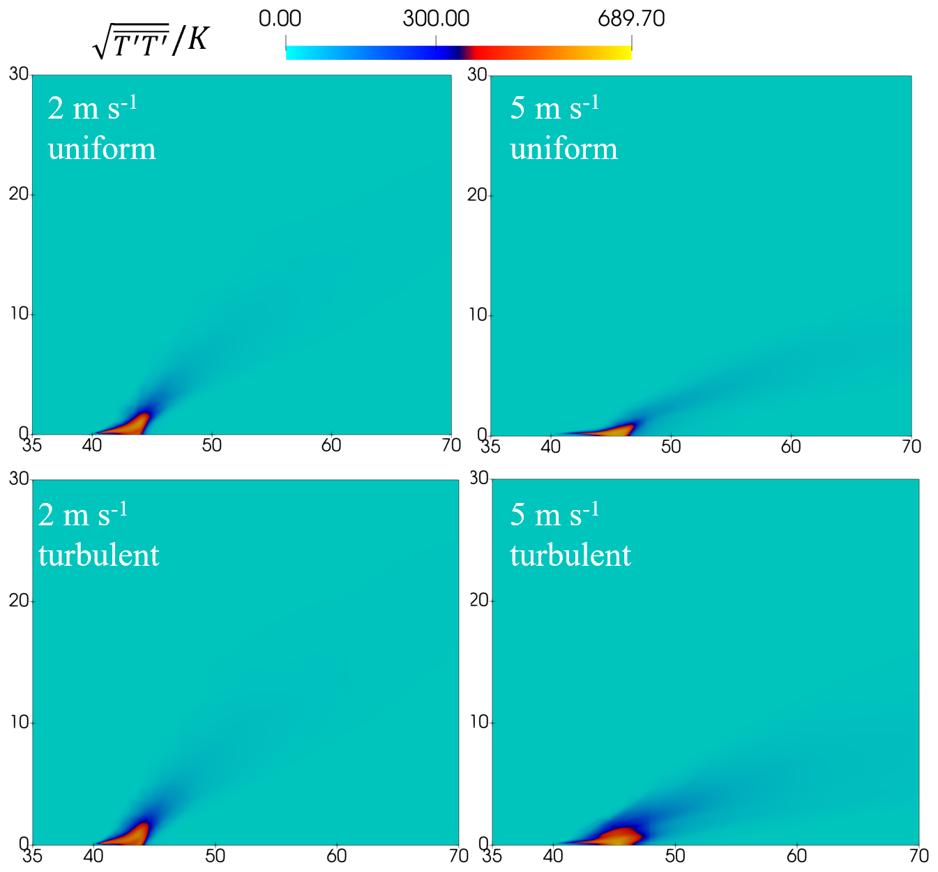
To further reveal the effect of approaching turbulence on the temperature variations, Fig. 13 compares root mean square (rms) of temperature fluctuations near the fire flame under different inlet conditions. For both velocities, rms of temperature is more inclined to downstream, similar to the mean temperature and velocity fields. However, there is a significant difference between two velocities. Under 2 m s⁻¹ condition, the distributions of rms of temperature are almost same and show a shoe-like pattern for uniform or turbulent inflow, with the latter case predicts smaller values. Flame is attached to the surface for both cases. Under 5 m s⁻¹ condition, patterns of the rms of the temperature are completely different for the uniform and turbulent cases. For uniform case, the pattern has a narrower region of large rms compared to that of 2 m s⁻¹ condition. For turbulent case, the pattern is completely different, with the high rms regions become wider and higher. This is maybe caused by the relatively large velocity fluctuations (as in Fig. 4) for this case, which breaks the steady flame structure that would exist in the uniform case and induce larger streamwise, spanwise and vertical momentum flux.

Figure 13 Mean temperature fluctuations near the fire under different inlet conditions.

To show the effect of inlet turbulence on the fire plume turbulent fluctuations, Fig. 14 compares the streamwise, spanwise and vertical velocity fluctuations under uniform and turbulent cases for $U_{\mathrm{0}}=\mathrm{2}\mathrm{m}{\mathrm{s}}^{-\mathrm{1}}$. Maximum values of three components are about 3.52, 1.95, and 9.38m² s⁻², with the vertical component has the largest value. Clearly, the turbulent fluctuations at this plane are dominated by the vertical and streamwise components. Three components have very similar structure for uniform and turbulent case, indicating that wind turbulence does not have significant influence on the fire plume turbulent structure, and it is mainly controlled by the buoyant force and mean wind force. However, their distributions are completely different for 5 m s⁻¹ condition, as shown in Fig. 15. For this inlet velocity condition, three components of velocity fluctuations are different between the uniform and turbulent cases. For the streamwise component, it is larger for turbulent case, with the maximum value reaches 2.09 m² s⁻², while it is only about 1.16 m² s⁻² for the uniform case. Moreover, it encompasses a larger region in turbulent case. For the spanwise component, the difference between the uniform and turbulent case is generally similar to that of the streamwise component. An additional large spanwise fluctuations are observed near the ground at X=47 m for the turbulent case, which means more spanwise momentum flux transport. For the vertical component, the maximum value is about 4.43 m² s⁻² and the turbulent case has a wider distribution.

Figure 14 Mean velocity fluctuations of the fire plume for $U_{\mathrm{0}}=\mathrm{2}\mathrm{m}{\mathrm{s}}^{-\mathrm{1}}$.

Figure 15 Mean velocity fluctuations of the fire plume for $U_{\mathrm{0}}=\mathrm{5}\mathrm{m}{\mathrm{s}}^{-\mathrm{1}}$.

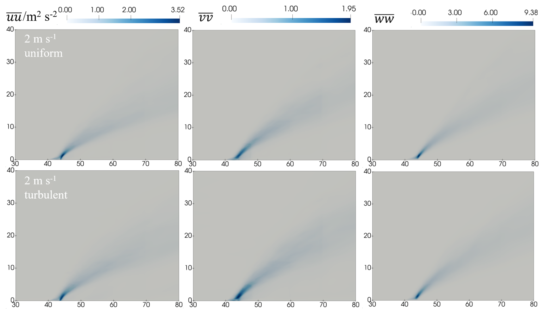
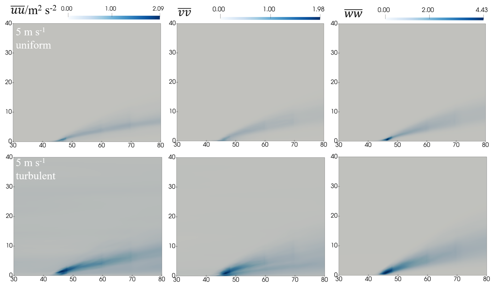
Figure 16 and 17 show the normalized turbulent kinetic energy (TKE) profiles along height at different X locations for U₀=2 and 5 m s⁻¹ respectively. The turbulent kinetic energy is calculated as $k=(\stackrel{\mathrm{‾}}{uu}+\stackrel{\mathrm{‾}}{vv}+\stackrel{\mathrm{‾}}{ww})/\mathrm{2}$. For the 2 m s⁻¹ condition, the TKE of the turbulent case is smaller at X=43 and 45 m. At further downstream, the TKE is always larger for the turbulent case. The TKE become larger at higher locations at further downstream, consistent with the plume rise. For the 5 m s⁻¹ condition, the TKE profiles show some different features. Firstly, the fire induced large TKE values are limited to a smaller range below Z=2 m before X=45 m, which is a consequence of stronger wind force. Secondly, the TKE of the turbulent case is always larger than that of the uniform case. This is partially because the approaching flow for this inlet velocity condition has a larger velocity fluctuation along the heights (as shown in Fig. 4). At downstream, the uniform and turbulent cases predict similar TKE profile pattern but the turbulent case has larger maximum values, which are almost as twice as that of the uniform case. Thirdly, significant differences of TKE maximums between X=43 and 45 m for the uniform and turbulent cases can be observed near the ground, with the turbulent case having larger values. This large turbulent kinetic energy can considerably alter the flow structure in this region and leads to different mixing and air entrainment here, which eventually cause the different temperature fluctuations (Fig. 13).

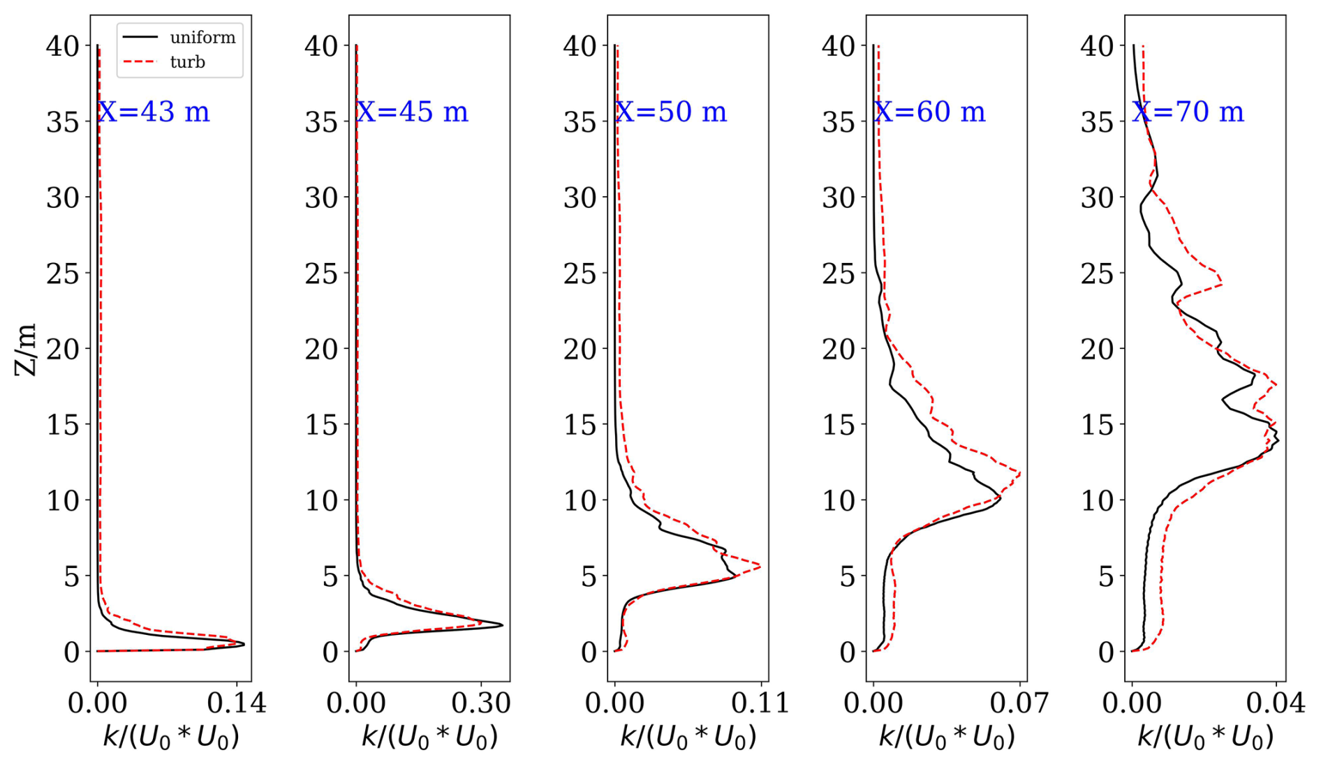
Figure 16 Turbulent kinetic energies (k) at different x locations for $U_{\mathrm{0}}=\mathrm{2}\mathrm{m}{\mathrm{s}}^{-\mathrm{1}}$. k is extracted from the middle Y plane.

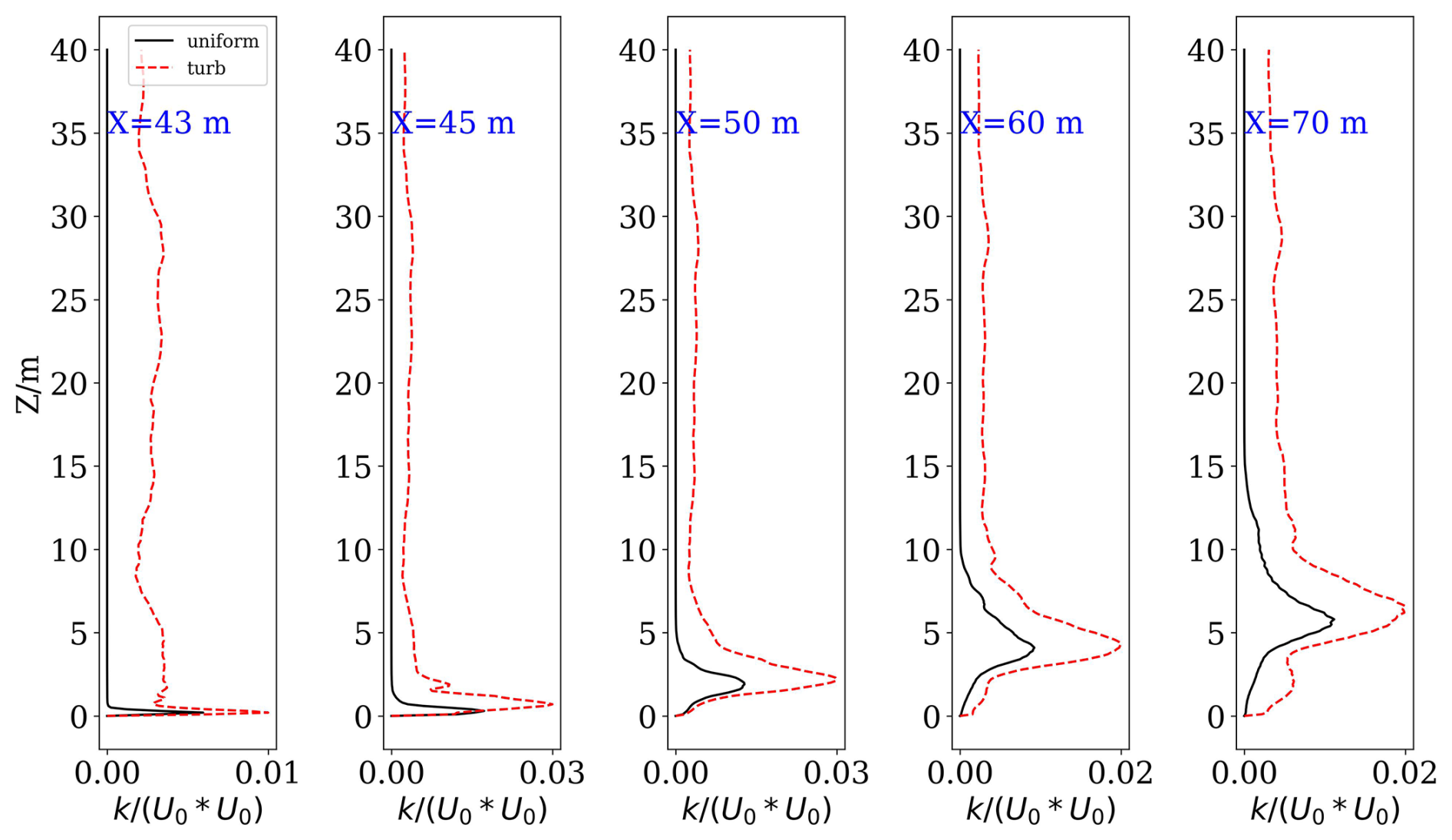
Figure 17 Turbulent kinetic energies (k) at different x locations for $U_{\mathrm{0}}=\mathrm{5}\mathrm{m}{\mathrm{s}}^{-\mathrm{1}}$. k is extracted from the middle Y plane.

4 Conclusions

The effect of inlet turbulence on the large eddy simulation of fire plume turbulent process is evaluated. This work aims to answer whether the approaching turbulence is important for the LES modelling of fire plume and at what extend it will affect the fire plume characteristics. Its effects are investigated for two background wind conditions, 2 and 5 m s⁻¹ at reference height. The approaching turbulence is generated by a divergence-free spectral representation method for the atmospheric boundary layer. We obtain the following conclusions:

1. The assumption of uniform flow does not have significant effect on the mean temperature and velocity fields for 2 m s⁻¹ case, but the plume height is slightly underestimated at downstream. However, it has larger effect for the 5 m s⁻¹ case, in which the temperature and velocity is largely under-estimated, especially at the downstream of the fire source. The maximum mean temperature difference can reach 50 K, and the mean velocity difference can reach 1.5 m s⁻¹.

2. For the mean temperature profiles and mean velocity profiles, the turbulent inflow condition leads to more smooth distributions at downstream, which indicates more momentum transfer in the vertical direction. It leads to slightly underestimation of mean and velocity at downstream for the 2 m s⁻¹ case and move obvious underestimation for the 5 m s⁻¹ case.

3. The assumption of uniform flow shows small effect on the temperature fluctuations near the flame for the 2 m s⁻¹ case, but large effect for the 5 m s⁻¹ case, in which the turbulent inflow leads to large temperature fluctuations near the rear end of the flame. This is associated with large turbulent kinetic energies near this region, which is relatively smaller for the 2 m s⁻¹ case. Differences of three components of fluctuations between the unform inflow and turbulent inflow case are also more obvious for the 5 m s⁻¹ case. This indicates that fire plume developed is more influenced by the background wind turbulence under relatively large velocity.

This work demonstrates the importance of inlet turbulence on the LES modelling of fire plume development near the ground. There are some limitations for this study. The approaching turbulent intensity is fixed and more investigations can be performed to obtain the dependence of the plume characteristics on the turbulent intensity under different velocities. The work is also limited to a flat surface, and its effect non-flat surface may vary because the terrain induced mechanical turbulence can be quite different. Due to the small size of the fire source, the plume rise is not high. For larger fire source, the plume rise may reach hundreds or thousands of meters, its development is further influenced by the stability of the atmosphere, which needs systematic investigations.

Appendix A

Figure A1 shows the effect of time averaging window size on the TKE distribution. It is clearly that the TKE changes little after 450 s, which means 240 s averaging is sufficient.

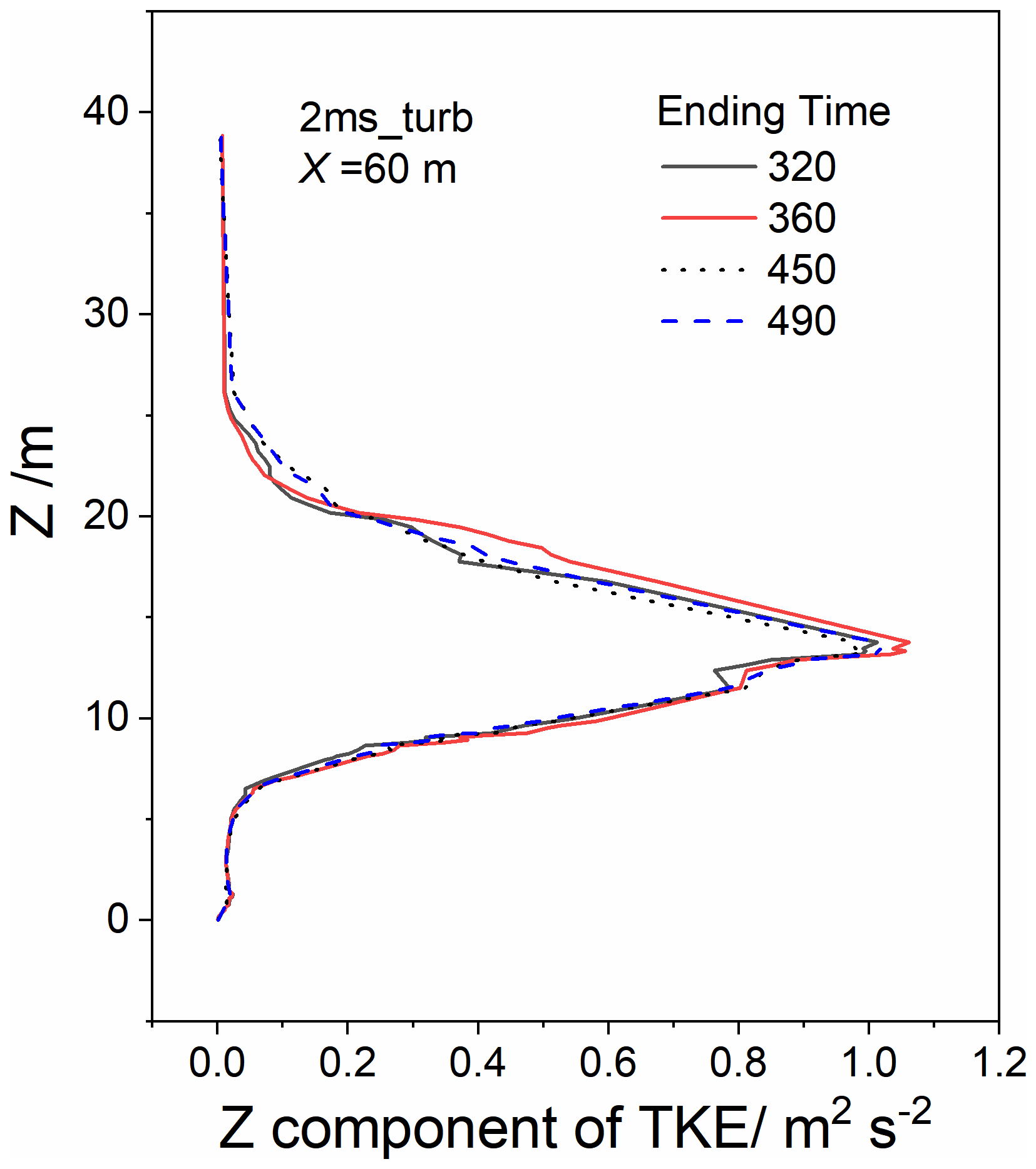
Figure A1 Effect of time averaging window on the TKE distribution at X=60 m for the 2 m s⁻¹ turbulent case