AIFS Single 1.1.0: an update to ECMWF's machine-learned weather forecast model AIFS

We present version 1.1.0 of ECMWF's Artificial Intelligence Forecasting System (AIFS Single), operational since 25 February 2025. The revised system introduces a bounding-layer framework that enforces physical constraints, such as non-negativity and internal consistency within precipitation and cloud cover variables, alongside expanded training data, revised loss weighting, and an extended set of surface and atmospheric variables. Overall skill improves by 4 %–6 % in the upper air and near-surface variables without degradation of spatial variability. A controlled comparison shows that training data expansion is the dominant source of upper-air skill gains, highlighting the importance of frequent model updates. The bounding framework delivers the largest precipitation improvements, up to 12 % and an approximately 1 d advantage using a categorical measure of skill. We further show that enforcing precipitation non-negativity resolves a gradient ambiguity at the zero-precipitation boundary under MSE training, explaining the reduction in drizzle bias and the improvements in precipitation.

1 Introduction

Machine-learned weather forecast models have started to rival or outperform physics-based numerical weather prediction (NWP) models in recent years (Pathak et al., 2022; Keisler, 2022; Lam et al., 2023; Chen et al., 2023; Bi et al., 2023; Lang et al., 2024a). For both training and forecasting, these machine-learned forecast models mostly depend on the Copernicus ERA5 reanalysis dataset produced by ECMWF (Hersbach et al., 2020) and operational analysis by ECMWF's physics-based integrated forecasting system (IFS).

ECMWF has developed the artificial intelligence forecasting system (AIFS) (Lang et al., 2024a), its own machine-learned forecast model. After a successful pre-operational test phase running four times daily since October 2023, with forecasts publicly available under ECMWF's open data policy, AIFS has now transitioned to operational status. The first operational version, AIFS 1.0.0 replacing AIFS 0.2.1, was implemented on 25 February 2025. The current operational version, AIFS 1.1.0 described here, was released on 27 August 2025 to correct a precipitation forecast issue in the initial version. The model is trained with a mean-squared error (MSE) loss function and is referred to as AIFS Single, to distinguish it from the probabilistically trained version, the AIFS ENS (Lang et al., 2024b).

Although such MSE-trained forecast models have been shown to smooth forecast fields at longer lead times to avoid the double-penalty of incorrectly positioned weather phenomena (Lam et al., 2023; Ben Bouallègue et al., 2024; Lang et al., 2024a; Bonavita, 2024; Brenowitz et al., 2025), they still display physically robust characteristics (Hakim and Masanam, 2024) and are able to make useful predictions of extreme events (Ben Bouallègue et al., 2024). The cheaper training costs associated with MSE-trained models (compared to probabilistically trained models) make them attractive for prototyping new features and model components.

To date, most machine-learned weather forecast models only include a limited subset of forecast variables available from current NWP systems. Here, we include for the first time in the AIFS soil moisture, soil temperature and runoff together with energy sector variables such as cloud cover, 100 metre winds and solar radiation. The choice of additional variables has been guided by utility to users and with considerations of future applications of the model, alongside pragmatic considerations on data availability and readiness. Surface solar radiation and 100-metre wind speeds have been included, important for renewable energy sectors. We added an initial characterization of the land surface with prognostic soil moisture and soil temperature, important for drought forecasting. We also include snowfall, improving the representation of distinct precipitation types in the model. Finally, we have added run-off as a diagnostic model output, pushing towards a hydrological component for the AIFS.

Despite their ability to produce skilful forecasts, machine-learned forecast models are prone to producing outputs that violate known physical relationships and limits (e.g., negative precipitation or mass imbalances). In current applications, including the pre-operational version of AIFS, post-processing of forecasts is commonly applied to remove such physical inconsistencies. Instead, we propose an additional final layer of activation functions that bound certain variables within physically meaningful limits and enforce physical constraints between related quantities. This simplifies the learning task by constraining the model output space to physically plausible regimes. This bounding strategy also proves particularly beneficial for variables with non-Gaussian distributions, such as precipitation, where the model must effectively distinguish between rain and no-rain states. Enforcing precipitation non-negativity resolves a gradient ambiguity at the zero-precipitation boundary under MSE training, greatly reducing drizzle bias and improving forecast skill in the light-precipitation regime.

In this paper we begin by outlining the training setup of the model and how this differs from the previous AIFS version. Then we motivate and describe the new bounding strategy to make the model forecast more physically consistent. We demonstrate the improved performance of the revised AIFS version via evaluation results and selected case studies. We conclude by summarizing main results and future work in the discussion and conclusions.

2 Training

The architecture of AIFS follows an encoder-processor-decoder design. Here, encoder and decoder are attention-based graph neural networks, and the processor is a transformer with a sliding window attention (see Lang et al., 2024a for details).

The model operates on a reduced Gaussian grid, (N320, approximately 0.25° resolution). The processor (or hidden) grid is an O96 octahedral reduced Gaussian grid (Wedi, 2014) with 40 320 grid points, approximately 1° resolution, and consists of 16 processor layers.

AIFS is trained to produce 6 h forecasts t_+6 h using past and present atmospheric states at $t_{-\mathrm{6},\mathrm{h}}$ and t₀ (from ERA5 or ECMWF's operational analyses at initialization, or from the model forecast itself). Longer lead times are produced auto-regressively by feeding the model's predictions back as inputs, a process commonly referred to as rollout.

2.1 Training schedule

The training is divided into two phases. The first is a pre-training phase, where the model learns to predict the atmospheric state 6 h ahead (t_+6 h) using ERA5 analysis at t_−6h and t₀. The second phase, rollout fine-tuning, continues from the pre-trained weights and trains the model to forecast auto-regressively up to 72 h. Here, the model learns to forecast from its own predictions. Unlike the previous AIFS version, where rollout fine-tuning was first performed using ERA5 and then followed by final fine-tuning on ECMWF operational analysis, we directly use operational analysis for the entire fine-tuning stage. This simplifies the training pipeline, reduces computational costs and is associated with improved forecast performance.

Pre-training is performed on ERA5 data covering the years 1979–2022 (compared to 1979–2020 in the previous AIFS version), using a cosine learning rate (LR) schedule, a batch size of 16, and a total of 260 000 training steps. The LR is linearly increased from 0 to $\mathrm{5}\times {\mathrm{10}}^{-\mathrm{4}}$ during the first 1000 steps, then annealed to a minimum of $\mathrm{3}\times {\mathrm{10}}^{-\mathrm{7}}$. This is followed by rollout fine-tuning on ECMWF operational analysis from 2016 to 2022, also using a cosine LR schedule and batch size of 16, for approximately 7900 steps (equivalent to one epoch per rollout step). The LR started at $\mathrm{1.28}\times {\mathrm{10}}^{-\mathrm{5}}$ and is annealed to the same minimum value of $\mathrm{3}\times {\mathrm{10}}^{-\mathrm{7}}$. The rollout length is initially set to 6 h (1 step) and progressively increased by one step per epoch up to 72 h (12 steps), following the approach of Lam et al. (2023) and Lang et al. (2024a). We used the AdamW optimizer (Loshchilov and Hutter, 2019) with β coefficients of 0.9 and 0.95. Here, the rollout dataset is extended to eight years of operational IFS analysis (2016–2022), compared with only 2 years (2019–2020) in the previous AIFS version.

Table 1 Variables used in the training of AIFS, with their short names, level type, variable type, normalization method, and scaling factors. Variables marked with ^* were newly introduced compared to AIFS v0.2.1.

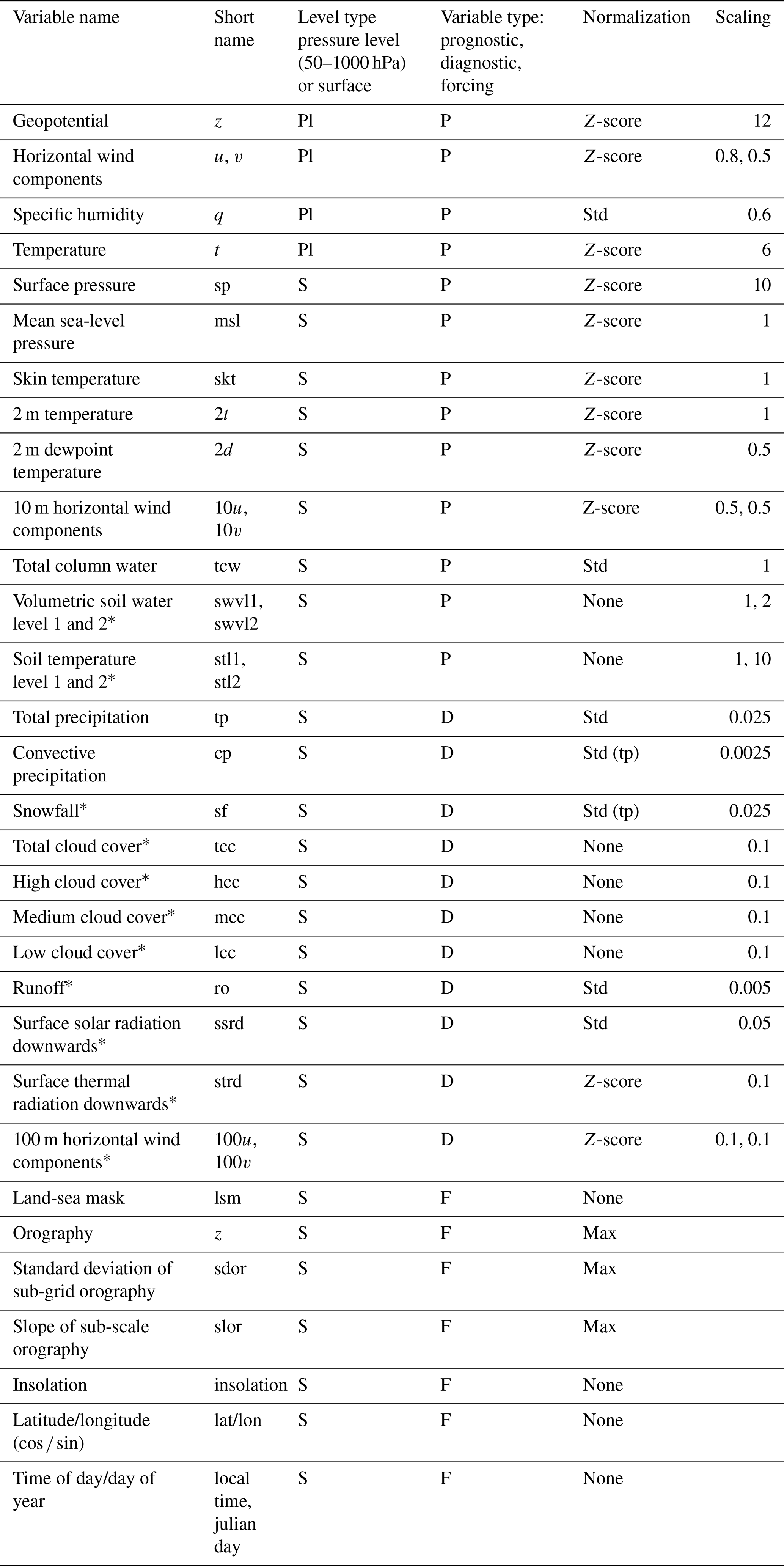
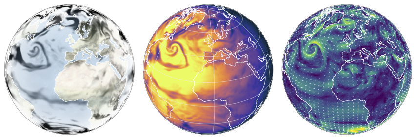
Figure 1 A selection of new variables available from the revised AIFS Single forecasts: cloud cover (left panel), surface solar radiation (centre panel), and 100 m wind speed/direction (right panel). The consistency between these new variables is clear, with areas of higher cloud cover corresponding to lower solar radiation at the surface and consistent weather patterns for 100 m winds.

2.2 Variables used in training

The variables used in the new AIFS version are listed in Table 1. As in AIFS 0.2.1, the upper atmosphere is represented by geopotential, horizontal wind components, specific humidity, and temperature at 13 pressure levels: 50, 100, 150, 200, 250, 300, 400, 500, 600, 700, 850, 925, and 1000 hPa. Newly introduced variables are marked with ^*. We have increased the characterization of the land surface in the model by including new prognostic variables of soil moisture at levels 1 and 2 (swvl1 and swvl2), and soil temperature at levels 1 and 2 (stl1 and stl2), important for drought monitoring and forecasting. A notion of hydrology has been included with runoff (ro), forecast as a diagnostic variable. A second set of variables, related to energy forecasting and clouds, adds real value to the model's utility. These are forecast diagnostically and include the 100 m wind components (100u and 100v), surface solar and thermal radiation (ssrd and strd), and cloud cover at various levels (tcc, hcc, mcc, lcc). Finally, snowfall (sf) has been added to complement the set of total precipitation-related variables. An illustration of a selection of these variables can be seen in the forecast presented in Fig. 1, where the consistency between these new variables is clear, with areas of higher cloud cover corresponding to lower solar radiation at the surface and consistent weather patterns for 100-metre winds. These new variables are sourced from the ERA5 reanalysis and IFS operational data archive, in line with those used in the previous AIFS version (0.2.1).

The per variable normalization strategy used in AIFS is summarized in Table 1. Unless stated otherwise, data is normalized to zero mean and unit variance (z-score normalization). For some bounded output variables (see Sect. 3), only standard deviation normalization is applied to avoid shifting of the absolute zero in the normalized space. The loss function is unchanged from the previous AIFS version. Table 1 shows the loss scaling factors we use in the revised AIFS version. Scaling factors were chosen empirically to ensure that all prognostic variables contribute approximately equally to the loss function, with the exception of vertical velocities and soil moisture, deliberately down-weighted. Vertical velocity is down-weighted due to known accuracy limitations in ERA5, particularly in convective regions. Soil moisture receives reduced weight for similar reasons, and additionally because the transition from ERA5-based pretraining to operational IFS analysis during fine-tuning introduces distributional inconsistencies; down-weighting mitigates the influence of this mismatch on training. Furthermore, the loss weights decrease linearly with height, so that upper atmospheric levels contribute less to the total loss. The pressure level weights are calculated following $w=\max (\mathrm{pressure}\mathrm{level}/\mathrm{1000}$, 0.2), like in the AIFS-ENS (Lang et al., 2024b). A minimum weight of 0.2 is imposed in the revised version to avoid assigning excessively low values in the stratosphere.

AIFS is trained using data parallelism with a batch size of 16, while each model instance is distributed across four GPUs within a single node (Lang et al., 2024a). Training was conducted on the European supercomputer Leonardo (EuroHPC), hosted and managed by Cineca, on 64 GB A100 GPUs. Mixed-precision training is used (Micikevicius et al., 2018), and the full process takes approximately 3 d. A 10 d forecast can be produced in about 2 min and 30 s on a single A100 40 GB GPU, including data input and output.

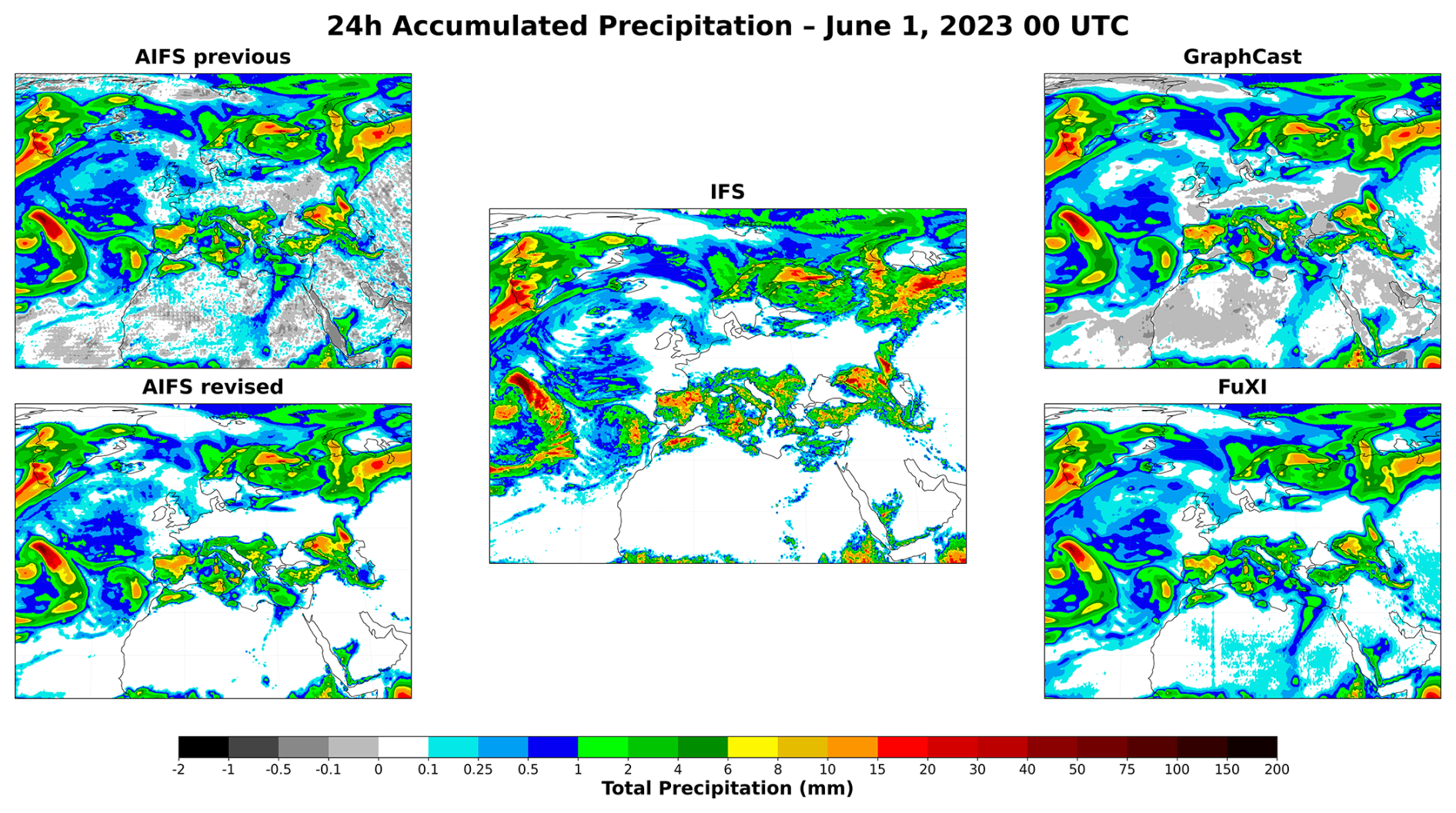
Figure 2 Comparison of 24 h total precipitation accumulation from five forecasting systems for the forecast issued at 1 June 2023 00:00 UTC and valid at 2 June 2023 00:00 UTC: previous AIFS, revised AIFS, operational IFS, GraphCast, and FuXi. The previous AIFS, GraphCast, and FuXi all exhibit an excess light rainfall, characteristic biases of ML weather models. The revised AIFS, incorporating the bounding layer framework, largely corrects the excess light precipitation issue and provides a precipitation distribution closer to the IFS reference in the light precipitation range.

3 Enforcing model constraints

Machine-learned forecast models for numerical weather prediction show very good forecast skill, yet they are prone to producing outputs that violate known physical laws or expected statistical consistency. Unlike traditional numerical models, which are governed by equations ensuring mass conservation, positivity, or energy bounds, machine-learned forecast models lack such guarantees by default. As a result, physically implausible outputs, such as negative precipitation, can emerge. We show that incorporating constraints into the model design to enforce physical realism improves forecast skill. In this section, we first identify specific issues in the output of the previous AIFS version related to total precipitation, and then introduce a simple yet effective method to bound the model outputs using activation functions. The proposed method is not restricted to total precipitation but can be equally applied to other variables.

3.1 Lack of physical realism in precipitation forecasts

The previous AIFS version suffers from significant drawbacks in forecasting precipitation. Most notably, the model's output is not constrained, leading to a frequent occurrence of negative values. This is illustrated in Fig. 2, which compares the 24 h accumulated total precipitation forecasts from the previous AIFS version, the revised version, GraphCast (Lam et al., 2023), FuXi (Chen et al., 2023) and an IFS (47r3) 24 h forecast, for the run initialized on 1 June 2023 at 00:00 UTC and valid at 2 June 2023 00:00 UTC. The previous AIFS model and GraphCast show spurious negative precipitation values, which are largely corrected in the revised AIFS. While negative values can be clipped to zero at inference time (as is done in FuXi in this figure and thus non visible), their presence highlights a lack of physical consistency in the model.

In addition to the negative values, a second noticeable issue, also visible in Fig. 2 and present for all the models but the AIFS revised version, is the excess of light precipitation in the forecast. The models produce excessive light rain leading to a bias in the forecast. Similar behaviour has been reported in benchmark studies such as WeatherBench 2 (Rasp et al., 2024), where AI-based systems including GraphCast, Pangu-Weather, and FuXi produce overly smooth precipitation fields and inflated frequencies of weak events, despite substantial architectural differences.

This is further supported by verification metrics computed against in situ observations (SYNOP stations). The Frequency Bias Index (FBI) scores for 2023 over Europe (Fig. 3) confirm that the pre-operational AIFS systematically over-forecasts light precipitation events (<1 mm). While a similar tendency is present in the IFS, it is considerably more pronounced in the machine-learned forecast model. At the other end of the distribution, the model tends to under-forecast more intense precipitation, as indicated by FBI values well below unity for thresholds exceeding 10 mm. This may be attributed to a well-known characteristic of machine learning-based forecasts: a tendency to produce overly smooth spatial fields, which can suppress extremes (Ben Bouallègue et al., 2024; Bonavita, 2024). Additionally, the coarser native resolution of AIFS (N320 0.25° grid) compared to IFS (0.1° grid) reduces its spatial representativeness.

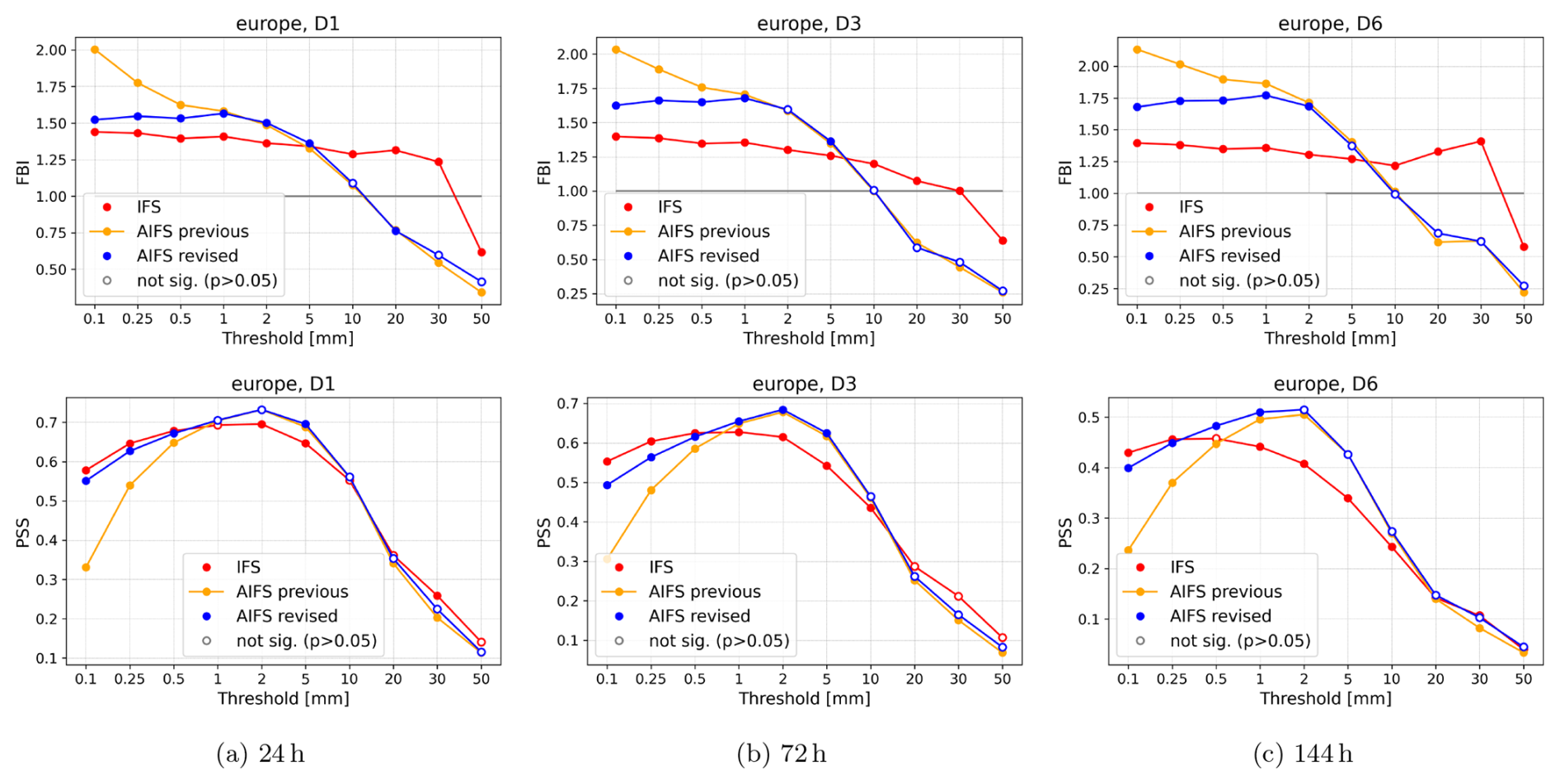
Figure 3 Frequency Bias Index (FBI, top panels) and Peirce Skill Score (PSS, bottom panels) for 24 h accumulated precipitation over Europe as a function of threshold, at forecast day 1, 3, and 6 (left to right panels). Scores are averaged over all initialisation dates in 2023. Filled markers indicate that the difference relative to the previous AIFS version is statistically significant (paired Wilcoxon signed-rank test, p<0.05); open markers indicate non-significant differences. The previous AIFS version exhibits a pronounced positive frequency bias at low thresholds, consistent with systematic overforecasting of light precipitation.

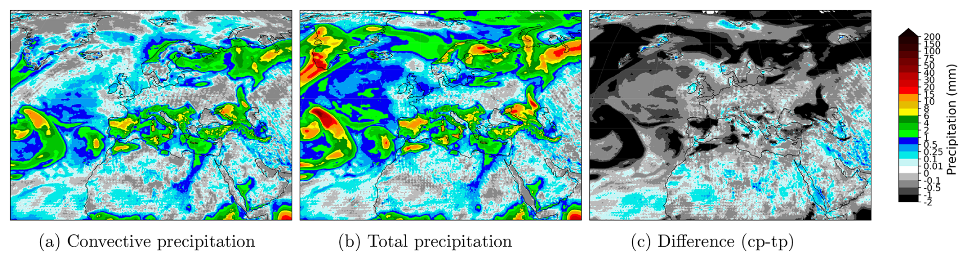
Figure 4 Comparison of 24 h total and convective precipitation forecast from the previous AIFS version, together with a map showing the difference between the two of them for the forecast issued at 1 June 2023 00:00 UTC and valid at 2 June 2023 00:00 UTC. Positive values (coloured regions) in the difference plot indicate areas where convective precipitation is greater than the total precipitation.

Convective precipitation forecasts also exhibit similar shortcomings. In addition, there is a further lack of physical consistency. Convective precipitation represents the part of the total precipitation that originates from convection, and therefore should always be less than or equal to the total. Figure 4 shows the previous AIFS 24 h accumulated forecasts of total and convective precipitation for 2 June 2023. The map displaying the difference between the two reveals frequent cases in which convective precipitation exceeds total precipitation, which should not occur.

The CREDIT platform (Schreck et al., 2025) has recently been used to explore physically informed constraints for addressing drizzle bias: Sha et al. (2025b) implemented global mass and energy conservation schemes as modular constraints within FuXi and demonstrated a direct reduction of drizzle bias; a companion study (Sha et al., 2025a) further showed that incorporating terrain-following (hybrid sigma-pressure) can improve extreme precipitation forecasts.

Here, we address the drizzle and negative precipitation issue through simplified intervention: enforcing only the physically admissible output range via a hard-constraint. This approach is described in Sect. 3.2. In Sect. 4.1, we show that this minimal architectural modification fundamentally reshapes the loss landscape in the vicinity of zero precipitation, eliminating gradient ambiguity and substantially reducing light-precipitation bias.

3.2 Bounding the outputs with activation functions

Precipitation has been used as an example to demonstrate the biases present in the forecasts of some variables. These issues are not only limited to precipitation, but are also observed in all sparsely distributed variables. This behaviour can be avoided by constraining the output of the model.

There are different strategies one could adopt to enforce physical constraints into the ML model. More specifically, here we tackled unphysical outputs, and we did not consider other constraints such as energy or mass conservation. Introducing loss penalties for outputs that fall outside the known physical bounds can be an effective strategy, and it has the advantage of not requiring any specific model change. Alternatively, the model could be modified in such a way as to prevent output from exceeding variable-specific physical bounds. This is usually referred to as hard-constraining. There are some examples in the literature of hard-constrained machine-learned models for climate and weather, such as Harder et al. (2024). The authors apply a softmax function, a generalization of the logistic function, as a hard-constraint for predicting quantities like atmospheric water content, to enforce the output to be non-negative in climate downscaling. Other examples can be found in Kent et al. (2025), Bonev et al. (2025) or Subramaniam et al. (2025). Similarly, we argue that hard constraints on the output can be enforced using an activation function.

Activation functions can be used in a straightforward way to enforce bounds in the output of machine-learned forecast models. Arguably, the most famous activation function and one we used in this work is the Rectified Linear Unit (ReLU), a nonlinear function defined as:

$$\begin{array}{}\text{(1)}& \mathrm{ReLU}\left(x\right)=\max (\mathrm{0},x).\end{array}$$

ReLU maps all negative values to zero, effectively enforcing a hard lower bound on the output.

For variables requiring both upper and lower bounds, such as concentrations or fractions, the Hard Hyperbolic Tangent (HardTanh) function is an effective choice. It is a piecewise linear approximation of the hyperbolic tangent, defined as:

$$\mathrm{HardTanh}\left(x\right)=\left\{\begin{array}{cl}\mathrm{0}& \mathrm{if}x<\mathrm{0}\\ x& \mathrm{if}\mathrm{0}\le x\le \mathrm{1}\\ \mathrm{1}& \mathrm{if}x>\mathrm{1}\end{array}\right..$$

HardTanh can also be used to enforce consistency between related output variables. For instance, consider the case of convective precipitation (Fig. 4), which is predicted independently of total precipitation in the previous AIFS version. There is a clear relation between the two quantities: convective precipitation is a fraction of total precipitation and should never exceed it. A more physically consistent approach is to map the original convective output to the [0, 1] range using a HardTanh layer and to multiply this output by the predicted total precipitation:

$$\begin{array}{}\text{(2)}& \mathrm{cp}=\mathrm{HardTanh}\left({\mathrm{cp}}^{\prime }\right)\times \mathrm{tp},\end{array}$$

where cp^′ is the convective precipitation output before the activation layer. This guarantees consistency. This type of constraint, referred to as FractionBounding, is applied to variables related to total precipitation and total cloud cover.

Clipping the precipitation output in inference is a possibility and a common practice. This was the case in the pre-operational AIFS model and also reported in other studies, such as Balogh et al. (2024). However, we show that the introduction of bounding in the output during training has benefits beyond simply avoiding slightly negative or unphysical values: it can facilitate the learning of forecasting for sparse and intermittent variables. Bounding effectively decomposes the prediction space into two distinct regions. In the case of total precipitation, the negative space becomes a proxy for forecasting the non-event, while the positive space corresponds to the occurrence of precipitation. This decomposition may, in principle, help the model more easily perform a classification between event and non-event outcomes, a distinction the previous AIFS version struggles with.

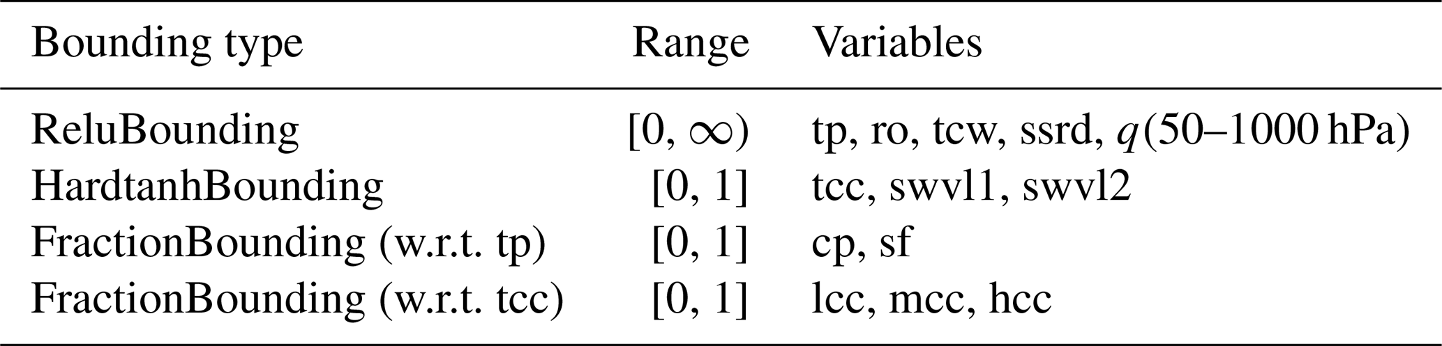
Table 2 summarises the bounding strategy used in the new version of the AIFS. Since bounding is performed on the normalized space, the choice of the normalization strategy is essential. In particular, variables bounded using a ReLU function were normalized using the standard deviation only, as indicated in Table 1, to avoid offsetting the zero value. Since snowfall and convective precipitation are predicted as fractions of total precipitation, it is necessary to ensure consistent magnitudes in the normalized space. Therefore, cp and sf were scaled using the standard deviation of total precipitation rather than their own. Total cloud cover and soil moisture variables (swvl1 and swvl2) were not normalized, since their range falls within the constraints imposed by the HardTanh bounding ([0, 1]).

Table 2 Summary of bounding strategies used in the new version of AIFS.

4 Evaluation

Unless otherwise stated, all verification results presented in this section are based on twice-daily forecasts initialised at 00:00 and 12:00 UTC for every day of 2023, verified against operational IFS analyses.

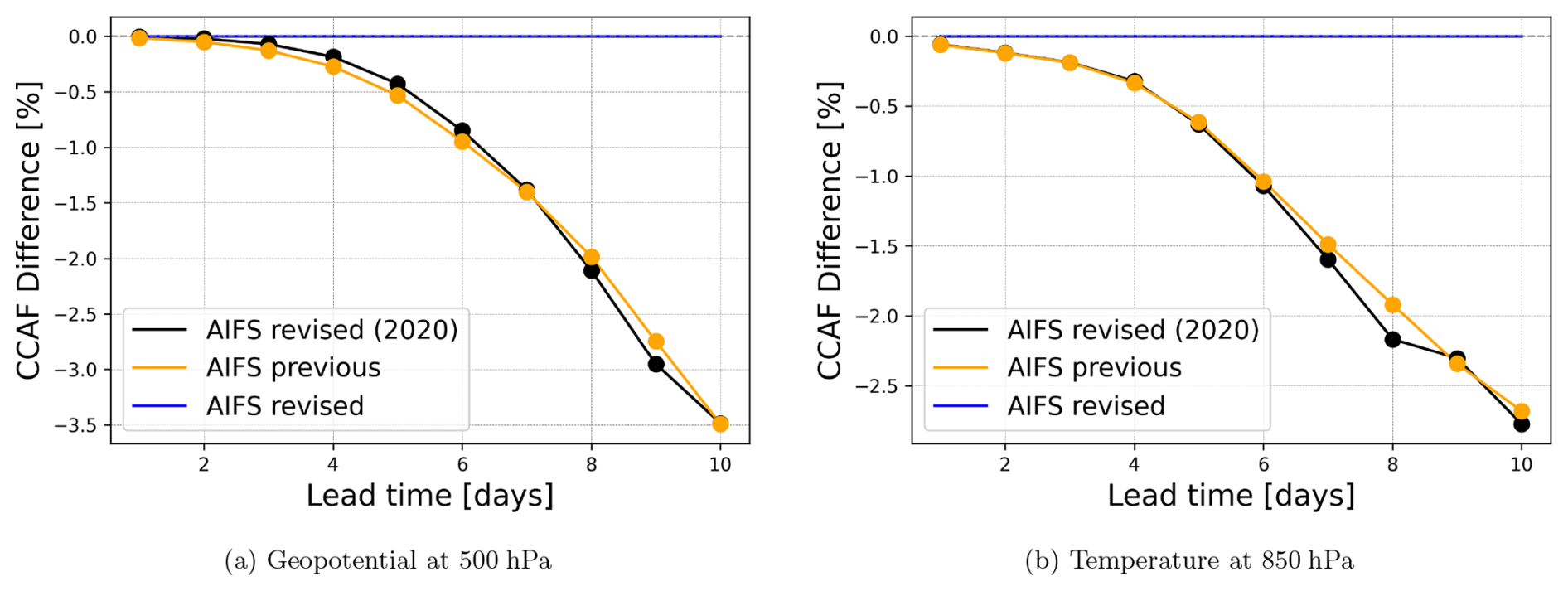
Figure 5 Anomaly correlation skill score difference for Geopotential at 500 hPa and Temperature at 850 hPa for 2023. This controlled comparison shows: (1) AIFS revised model (full system with all modifications), (2) AIFS revised trained with limited data (ERA5 up to 2020, rollout fine-tuning 2019–2020 only), and (3) AIFS previous version. The close agreement between configurations (2) and (3) demonstrates that the substantial performance gain is primarily attributable to the expanded training dataset (ERA5 1979–2022 and rollout data 2016–2022). Solid points indicate statistically significant differences relative to AIFS revised used as reference (paired Wilcoxon signed-rank test, p<0.05).

The revised AIFS version delivers highly skilled forecasts, as shown by anomaly correlation scores for 2023 in the Northern Hemisphere (Fig. 8). In the medium range (3–10 d), AIFS outperforms the IFS by 12 to 24 h in skill. Forecast skill is also clearly improved compared to the previous AIFS version. This performance gain can be attributed to the combined effect of increased training data, improvements in rollout fine-tuning, the implementation of output bounding, and the inclusion of new prognostic variables. To quantify the specific contribution of expanded training data, we present a controlled comparison in Fig. 5. We verify against the operational IFS analysis, which is also used to initialise the forecasts.

As shown in Fig. 5, the expanded training dataset contributes to the most important portion of the overall performance gain. This indicates that data availability (ERA5 extended to 2022 and rollout fine-tuning expanded from 2019–2020 to 2016–2022) plays a major role. The remaining improvement stems from other system modifications, including rollout fine-tuning schedules, output bounding layers, and expanded prognostic variables. Due to the high computational cost, a detailed ablation study to isolate the impact of each individual modification beyond data expansion was not performed; thus, the observed improvements represent the cumulative result of these integrated system updates. It should be noted that the close agreement between AIFS revised (2020 data) and AIFS previous in ACC should be interpreted with caution, as these configurations differ in their training protocols: AIFS previous includes a rollout fine-tuning phase on ERA5 which AIFS revised (2020) does not, and uses only 2 years (2019–2020) of operational data for final rollout fine-tuning compared to 6 years (2016–2022) in the full revised version. Furthermore, similar ACC scores do not imply equivalent forecast quality. As shown in Fig. 6, AIFS revised (2020) exhibits less mesoscale smoothing than AIFS previous despite comparable ACC, indicating that the changes introduced in the revised system do contribute positively to forecast quality in ways not fully captured by ACC alone.

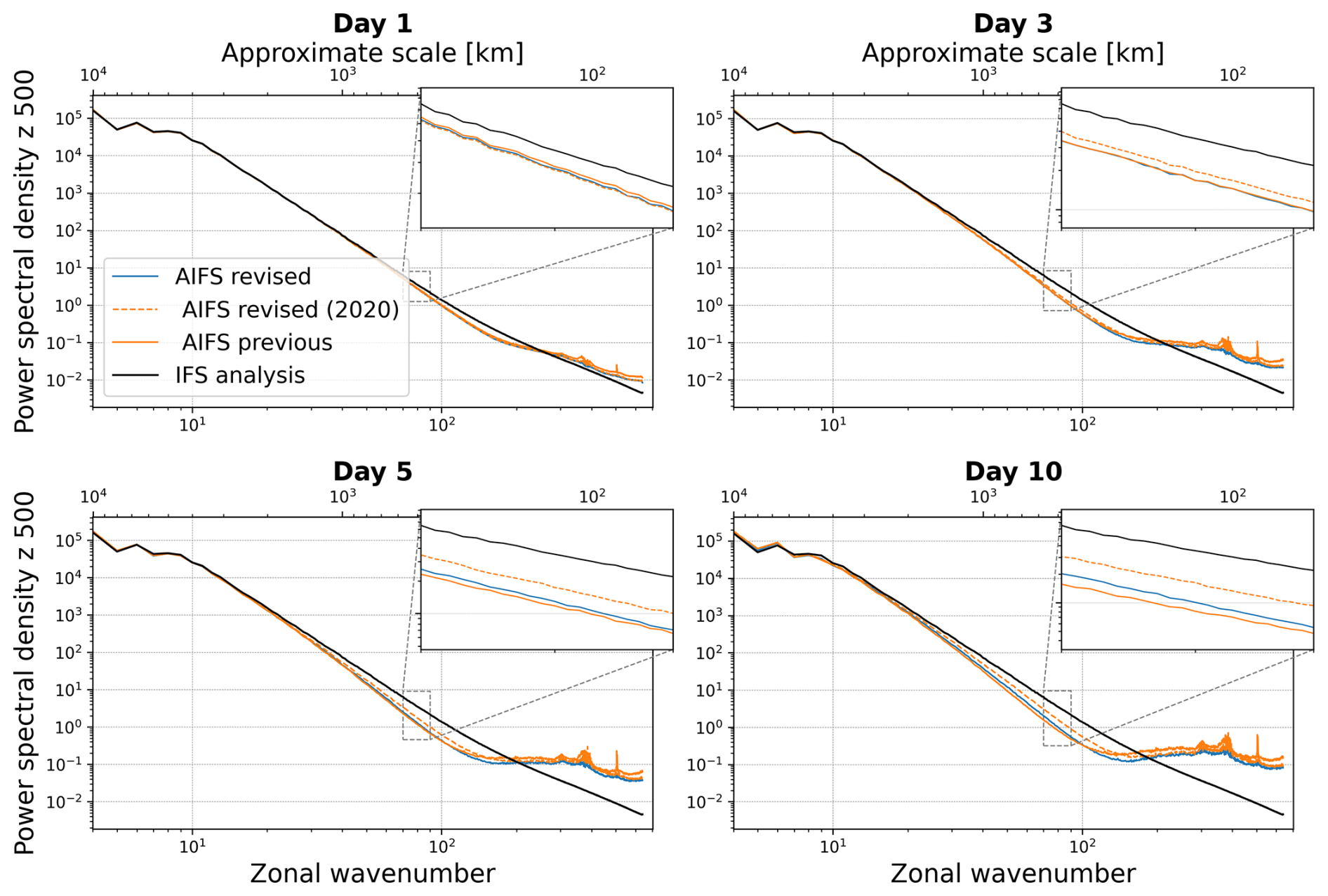
Figure 6 Z500 power spectral density as a function of zonal wavenumber (bottom axis) and approximate horizontal scale in km (top axis) for forecast lead times Day 1, 3, 5, and 10 during JJA 2023. Spectra from the revised AIFS (blue), AIFS revised trained with limited data (ERA5 up to 2020, rollout fine-tuning 2019-2020 only) in dashed orange, and previous AIFS (orange) are compared against the IFS analysis (black). Insets highlight the 450–600 km scale range (zonal wavenumbers 70–90), corresponding to large mesoscale structures. The revised AIFS shows improved agreement with the IFS analysis at large mesoscale structures, particularly at longer lead times, indicating a better representation and retention of mesoscale variance.

Additionally, imposing a minimum on the loss weights in the stratosphere leads to significant improvements in the data-driven forecasts at 100 and 50 hPa (Fig. 9). For temperature at 100 hPa, the new version of the AIFS outperforms the IFS, while for 50 hPa wind speed, the gap in skill between the previous version of AIFS and the IFS in the stratosphere is significantly reduced.

Forecast skill for key surface variables, such as 2 m temperature and 10 m wind speed, verified against SYNOP observations, is similarly improved (Fig. 10). Overall, the new AIFS version exhibits improvements of around 4 %–6 % across all variables, lead times, and pressure levels relative to the previous AIFS version, as shown in the scorecard presented in Fig. 7. The performance of the model for tropical cyclone prediction is similar to that of the previous version (see Lang et al., 2024a), with some small improvements to track position. The training configuration, including a maximum rollout length of 12 (72 h), was retained from the previous AIFS version, as shown in Sect. 2.1. This parameter is known to influence spectral characteristics, with longer rollouts leading to enhanced damping. No explicit tuning was performed to target spectral behaviour.

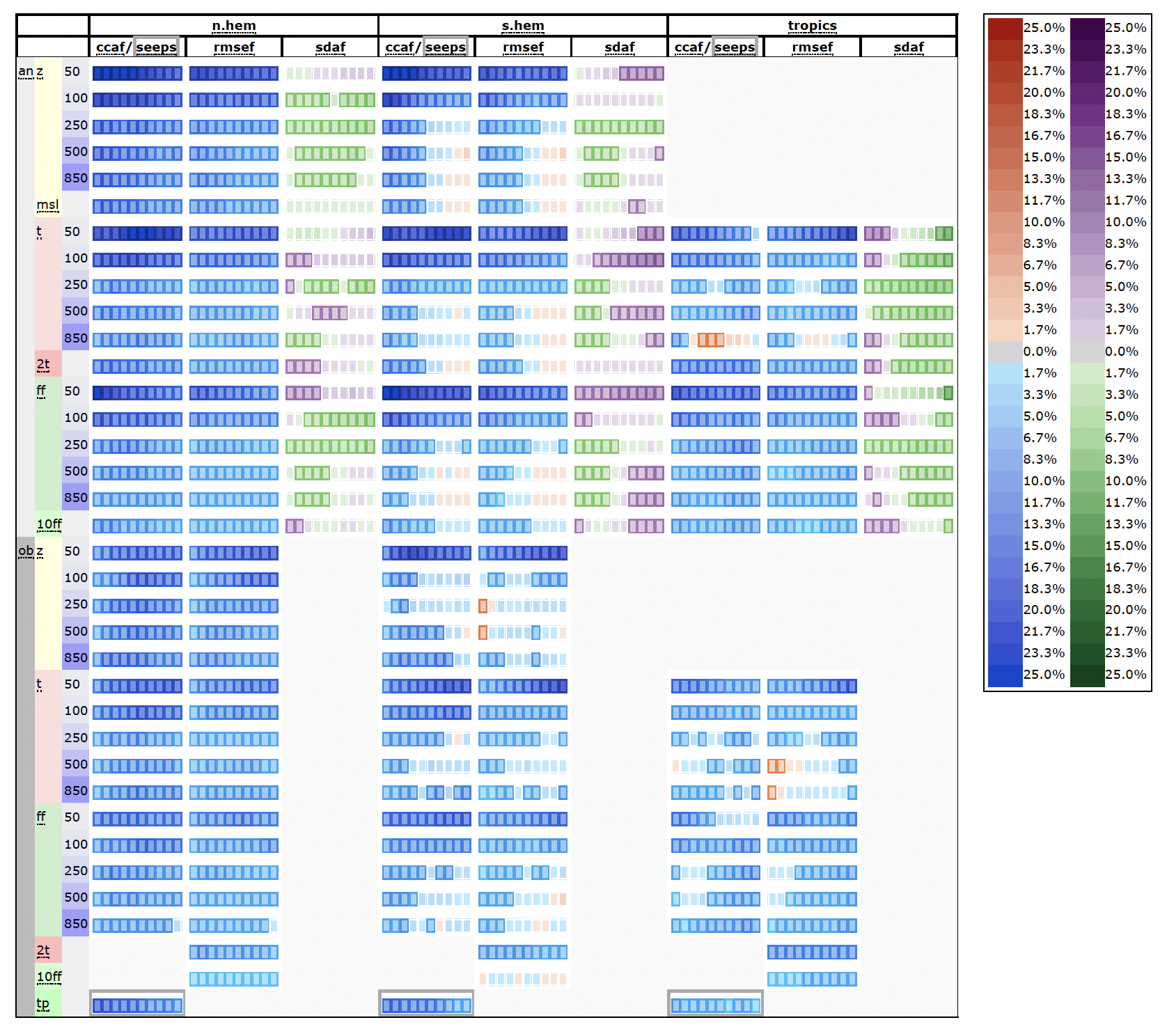
Figure 7 Scorecard comparing forecast scores of AIFS revised versus the previous AIFS version for the whole year of 2023. Forecasts are initialised on 00:00 and 12:00 UTC. Relative score changes are shown as function of lead time (day 1 to 10) for northern extra-tropics (n.hem), southern extra-tropics (s.hem) and tropics. Blue colours mark score improvements and red colours score degradations. Purple colours indicate an increased in standard deviation of forecast anomaly, while green colours indicate a reduction. Framed rectangles indicate 95 % significance level. Numbers behind variable abbreviations indicate variables on pressure levels (e.g., 500 hPa), and suffix indicates verification against IFS NWP analyses (an) or radiosonde and SYNOP observations (ob). Scores shown are anomaly correlation (ccaf), SEEPS (seeps, for 24 h precipitation accumulation), RMSE (rmsef) and standard deviation of forecast anomaly (sdaf).

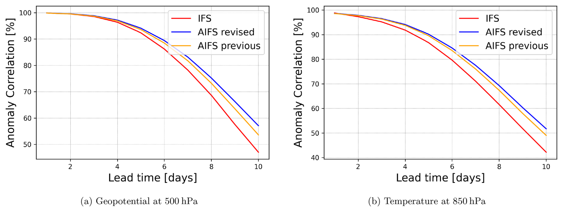
Figure 8 Anomaly correlation skill scores for geopotential and temperature at 500 and 850 hPa, respectively. Skill scores computed for the Northern Hemisphere for the whole of 2023 against IFS analysis. In the medium range, AIFS revised outperforms the IFS by 12 to 24 h in skill. Forecast skill is also clearly improved compared to the previous AIFS version.

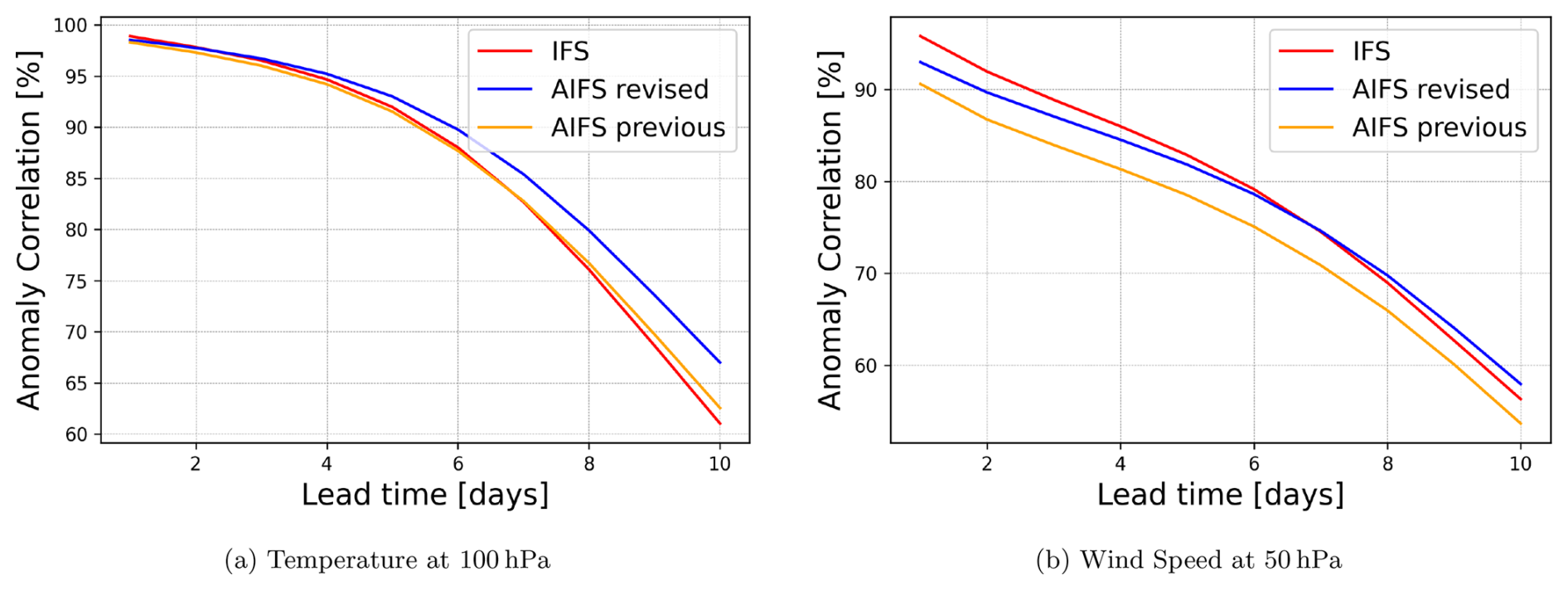
Figure 9 Anomaly correlation skill scores for temperature at 100 hPa and wind speed at 50 hPa. Skill scores computed for the Northern Hemisphere for the whole of 2023 against IFS analysis. Significant improvements in the revised AIFS forecasts at 100 and 50 hPa when compared against the previous AIFS version.

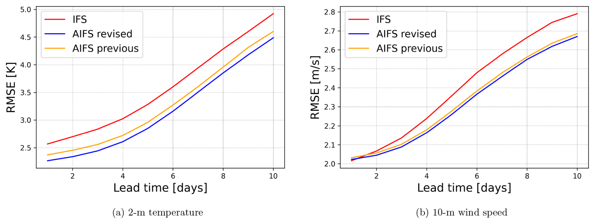
Figure 10 RMSE scores for 2 m temperature and 10 m wind speed computed against SYNOP observations over the Northern Hemisphere. The revised AIFS version shows improvement when compared to the previous verision of the AIFS.

The resulting Z500 power spectral density shown in Fig. 6 are very similar to those of the previous AIFS across scales, including the ∼500 km range (zonal wavenumbers 70–90), with slightly improved agreement with the IFS analysis at longer lead times. At the same time, the RMSE-based scorecard (Fig. 7) shows overall improvements. Taken together, these results indicate that the skill gains are not achieved at the expense of degraded spatial variability.

Figure 11 presents verification metrics for several variables introduced in the new version. In line with those already present in earlier versions, AIFS shows a gain in forecast skill of around 1 d in the medium range for surface short-wave downwards radiation verified against geostationary satellite observation via CMSAF (Pfeifroth et al., 2023) and 100 m wind speed verified against ECMWF operational analysis, relative to the IFS. The population distribution for total cloud cover verified against SYNOP observations, however, highlights the inherent limitations of MSE-trained AI models. While the observed distribution follows a U-shape, with high frequency at the tails of the distribution (clear skies and overcast conditions), AIFS produces a much flatter distribution, under-predicting these extremes and over-estimating intermediate values. This behaviour is closely linked to the smoothing effect introduced by the MSE loss function, which tends to penalize large deviations and thereby suppress extremes (see Sect. 5).

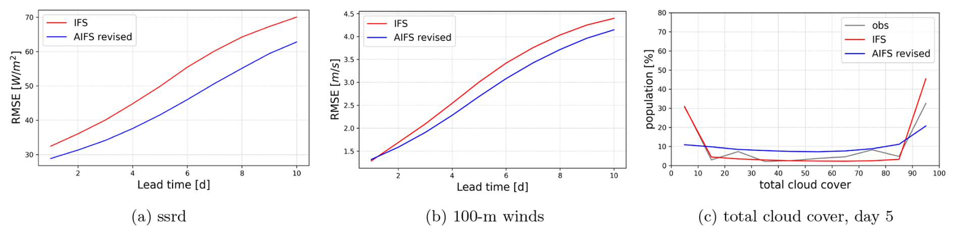
Figure 11 Forecast RMSE computed against operational IFS analysis and distribution comparison for new variables. (a) Surface solar radiation downwards RMSE for March–May (MAM) 2023, (b) 100 m wind speed RMSE for the full year 2023, (c) total cloud cover distribution for June–August (JJA) 2023. Blue lines show the AIFS revised and red lines show IFS; observations are shown in grey in panel (c). AIFS shows significant gains in forecast skill in the medium range for surface short-wave downwards radiation and 100 m winds when compared against the IFS. The mismatch in population distribution for total cloud cover forecast highlights the inherent limitations of MSE-trained AI models.

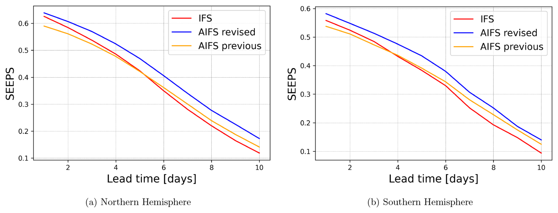
Figure 12 SEEPS skill scores for 2023 based on 24 h accumulated precipitation from SYNOP observations, comparing the revised AIFS (blue), the previous AIFS version (orange), and the IFS (red) across different regions. Results show a consistent and statistically significant improvement across all lead times and in the Northern Hemisphere and the Southern Hemisphere for the revised AIFS version when compared to the previous AIFS version and the IFS.

The forecasting skill of the model with respect to 24 h accumulated total precipitation is significantly improved. The new AIFS version is compared against both the previous AIFS version and the operational IFS (cycles 47r3 and 48r1) in Fig. 12. The Stable Equitable Error in Probability Space (SEEPS) skill score (Rodwell et al., 2010) is used as the primary verification metric, with 24 h accumulated precipitation SYNOP observations serving as the reference. Results show a consistent and statistically significant improvement across all lead times and in the Northern Hemisphere and the Southern Hemisphere. The revised AIFS demonstrates approximately a 1 d gain in forecast skill relative to both IFS and the previous AIFS version. The forecast fields also exhibit noticeable improvements, as illustrated in Fig. 2. The new version of the AIFS produces no negative values in the output and substantially reduces light precipitation, aligning more closely with the 24 h total precipitation accumulation fields derived from the IFS operational short-range forecasts.

Figure 3 reveals where the improvement originates. The Frequency Bias Index (FBI, Wilks, 2019), defined as the ratio of predicted to observed event frequency at a given threshold ($\mathrm{FBI}=(H+\mathrm{FA})/(H+M)$, where H are hits, FA false alarms, and M misses), and the Peirce Skill Score (PSS, also known as the Hanssen–Kuipers discriminant; Jolliffe and Stephenson, 2011), defined as the difference between the probability of detection and the probability of false detection ($\mathrm{PSS}=H/(H+M)-\mathrm{FA}/(\mathrm{FA}+\mathrm{CN})$, where CN are correct negatives), are shown for the Northern Hemisphere for different thresholds. The previous AIFS version exhibits a strong tendency to over-predict light precipitation events (<1 mm) across all lead times, as shown by the FBI. This bias is substantially corrected due to the bounding (see Sect. 4.1) in the revised AIFS.

While the AI model still slightly over-predicts light precipitation compared to the IFS, it demonstrates competitive skill for light precipitation. The AIFS excels at medium-intensity events (1–10 mm), with PSS scores significantly higher than those of the IFS. At higher thresholds (>10 mm), corresponding to moderate to heavy precipitation, the AIFS diverges from the IFS, with a marked under-prediction (FBI < 1). This is likely caused by smoothing introduced by the loss function, in combination with the model’s coarser spatial resolution.

This under-prediction plays an important role in the metrics concerning more extreme events, since both the previous and the revised AIFS models underperform IFS for thresholds exceeding 10 mm in terms of PSS, but remains competitive. This suggests that although the AI models predict fewer high-intensity events, their predictions are more accurate when they do occur. Finally, the revised AIFS shows a marginal improvement in terms of PSS compared against the previous AIFS version, possibly due to improvements in the learning-rate scheduling used for fine-tuning and additional training data.

4.1 Evaluating the effects of bounding on total precipitation

Overall, the revised AIFS version demonstrates significant improvements in forecasting skill for total precipitation over its predecessor. The bounding of total precipitation transforms the prediction space such that negative values correspond to “no-rain” and positive values to “rain”. This separation enables the model to more effectively distinguish between the two scenarios. It removes the pressure to forecast exactly zero and facilitates the classification task inherent to precipitation forecasting.

Other factors that might improve the precipitation forecast skill in the revised AIFS version are the inclusion of additional variables, the improved learning rate scheduling for rollout fine-tuning and the expansion of the training dataset. To isolate the effect of the bounding mechanism, we retrained the revised AIFS version using the exact same training configuration and data extent, with the sole exception of omitting the bounding layer for total precipitation. This controlled baseline, hereafter referred to as “AIFS revised no-bounding”, allows for a direct comparison between the two models. The SEEPS skill score for the June-July-August 2023 season is shown in Fig. 13. The results show that the improvement observed in total precipitation forecast skill in the revised AIFS version can mainly be attributed to constraining the output, since the revised AIFS version without bounding performs similarly to the previous AIFS version.

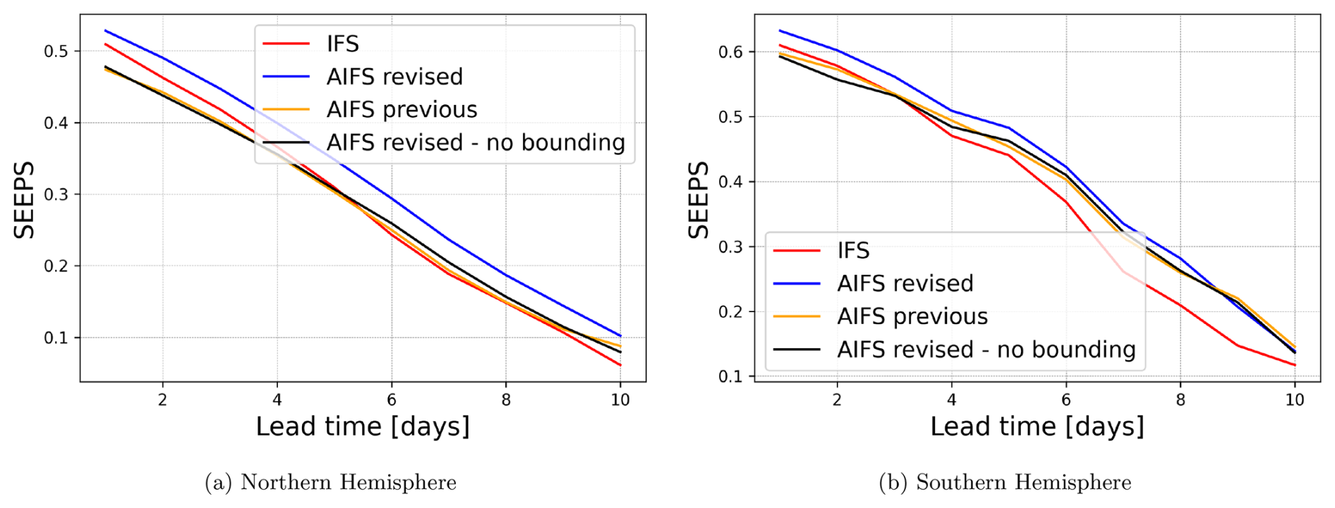
Figure 13 SEEPS skill scores for 2023 JJA comparing revised AIFS (blue), revised AIFS without bounding (black), previous AIFS (orange), and IFS (red) across different regions. The improvement observed in total precipitation forecast skill in the revised AIFS version can mainly be attributed to bounding the output of the model.

The physical consistency of convective precipitation forecast in respect to total precipitation can also be evaluated for a given forecast to assess the utility of the FractionBounding strategy used. Figure 14 presents the 24 h total and convective precipitation accumulation together with a map showing the difference between the two for a forecast issued at 1 June 2023 00:00 UTC and valid at 2 June 2023 00:00 UTC. Unlike the previous AIFS version (Fig. 4), the convective precipitation forecast is now consistent with the predicted total precipitation accumulation.

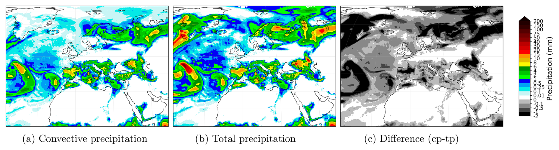
Figure 14 Comparison of 24 h total and convective precipitation accumulation forecast from the revised AIFS version, together with a map showing the difference between the two of them for the forecast issued at 1 June 2023 00:00 UTC and valid at 2 June 2023 00:00 UTC. Unlike the previous AIFS version (Fig. 4), the convective precipitation forecast is now consistent with the predicted total precipitation accumulation and no coloured regions (cp > tp) appear in the difference plot.

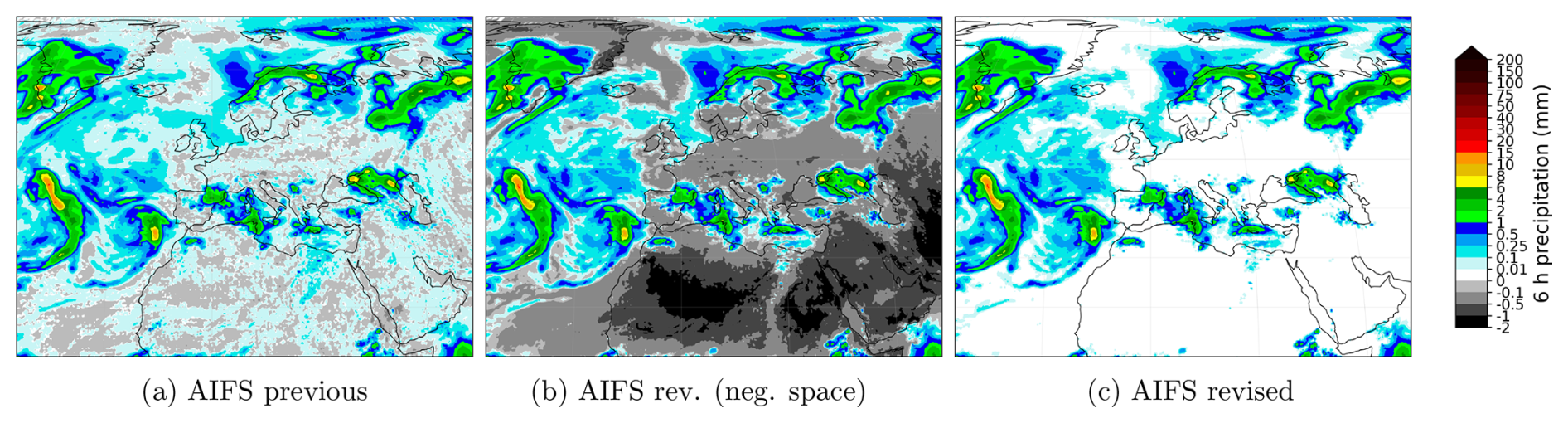
Figure 15 Comparison of 6 h total precipitation from previous AIFS, revised AIFS without the final ReLU layer to show the negative space, and the standard revised AIFS with the final ReLU layer. Forecasts are initialised at 1 June 2023 00:00 UTC and valid at 1 June 2023 06:00 UTC. Removing the final bounding layer from the AIFS revised model reveals the behaviour of the negative space for the total precipitation variable. The model has implicitly learned to use the negative space as a proxy for “no-rain” classification.

To better understand the mechanisms governing total precipitation forecasts in the revised AIFS configuration, we examine the model's behaviour in the negative pre-activation space obtained by removing the final ReLU layer at inference. Figure 15 reveals that this nominally hidden negative space is neither random nor noisy, but highly structured.

At first glance, bounding an output variable with a ReLU activation may appear to introduce a drawback: the negative pre-activation space is not directly penalized, since all negative values are projected to zero before the loss is evaluated. In principle, changes within this region do not influence the weight updates. One might therefore expect the negative space to be uninformative or unstable.

Instead, we observe a coherent and physically meaningful organization. Persistently dry regions, such as the Sahara Desert, exhibit strongly negative pre-activations, while areas approaching precipitation events transition smoothly toward zero. The model has therefore learned to encode dryness in the negative space, effectively using it as a latent representation of the “no-rain” regime.

This observation motivates two fundamental questions:

• i.

  why does the negative pre-activation space contain coherent and physically meaningful structure, and

• ii.

  why does enforcing a non-negativity constraint during training improve light-precipitation skill?

We argue that the first arises from the shared latent representation of the atmospheric state learned by the network, while the second is governed by the symmetry properties of the MSE gradient near the zero-precipitation boundary.

4.1.1 Representation of dry states in the negative space

In this study we argue that the structure present in the negative space is an emergent feature arising from the shared representation of atmospheric states.

The model encodes input prognostic (X_t) and forcing variables (F_t) into a high-dimensional latent space (z_t) via an encoder:

$$\begin{array}{}\text{(3)}& z_t=\mathrm{Encoder}\left({\mathbf{X}}_t,{\mathbf{F}}_t\right).\end{array}$$

This latent state is evolved to the next time-step through the processor (e.g., via attention-based computations):

$$\begin{array}{}\text{(4)}& z_{t+\mathrm{6}}=\mathcal{F}\left(z_t\right)\end{array}$$

and then decodes back into the physical space to obtain the forecast at t+6 of prognostic (X_t+6) and diagnostic (D_t+6) variables. It is worth mentioning here that z_t+6 encodes the physical state of all the prognostic variables in a shared representation space and the diagnostic variables are decoded from it. The diagnostic precipitation output is thus produced by a specific decoder head:

$$\begin{array}{}\text{(5)}& {\mathit{\eta }}_{t+\mathrm{6}}={\mathrm{Decoder}}_{\mathrm{tp}}\left(z_{t+\mathrm{6}}\right)\end{array}$$

where η represents the pre-activation total precipitation. The final physical output is obtained via the bounding layer:

$$\begin{array}{}\text{(6)}& {\mathrm{tp}}_{t+\mathrm{6}}=\mathrm{ReLU}\left({\mathit{\eta }}_{t+\mathrm{6}}\right)=\max \left(\mathrm{0},{\mathit{\eta }}_{t+\mathrm{6}}\right).\end{array}$$

Because Decoder_tp maps from a latent space optimized for smooth gradients (z_t+6), η inherits this spatial structure. The precipitation decoder head learns a smooth mapping from the latent space encoding the moisture state of the system to physical precipitation in the positive regime (η>0), where gradients are active. Because neural networks are continuous functions biased toward smoothness, this “moisture-to-precipitation” logic naturally extrapolates into the negative regime. As moisture variables decrease, the decoder continues to output decreasing values, pushing η into the negative space.

While the precipitation head receives no direct gradients when η<0, the latent variables that serve as its input are not static. These latent features are shared with prognostic variables (e.g., specific humidity q, total water content tcw, etc) and receive continuous gradient information from their respective loss functions. Consequently, the negative space of the tp field is “indirectly learned”; it is a projection of a latent space that is being rigorously optimized.

Ultimately, this reveals that the optimization of the shared latent space is driven by the collective constraints of all output variables. In this framework, the negative pre-activation space for precipitation serves as a “saturation deficit” proxy that is kept physically consistent by the gradients flowing from prognostic moisture fields. The shared representation of the atmosphere in the latent space allows the model to maintain a sophisticated, structured representation of dryness even in the absence of direct precipitation gradients.

To provide empirical weight to this mechanistic theory, we investigate the information content within the pre-activation space η by partitioning the model output into three distinct physical regimes: the negative (non-precipitating) space, the light precipitation regime (0–0.5 mm per 6 h), and the moderate precipitation regime (0.5–10 mm per 6 h).

We hypothesize that the pre-activation space η undergoes a fundamental physical decoupling as it transitions from dry to wet conditions. In the negative (non-precipitating) regime, the absence of precipitation is a deterministic function of low humidity; thus, the decoder should preserve a strong linear mapping from the prognostic moisture fields.

Conversely, we expect this linear correlation to weaken in the light precipitation regime ($\mathrm{0}<\mathit{\eta }\le \mathrm{0.5}$ mm). While moisture remains a necessary condition for rain, the exact accumulation at these low intensities becomes increasingly stochastic, influenced by non-linear factors such as sub-grid scale turbulence, cloud-base evaporation, and microphysical uncertainties. These processes act as “interference”, decoupling the surface precipitation from the column moisture signal.

We performed a global correlation analysis on a single forecast issued at 1 June 2023 00:00 UTC. For this experiment, we utilize the AIFS revised model without the final bounding layer on tp during inference, but activated during training. We focus our analysis on the first 120 h (5 d) of the forecast.

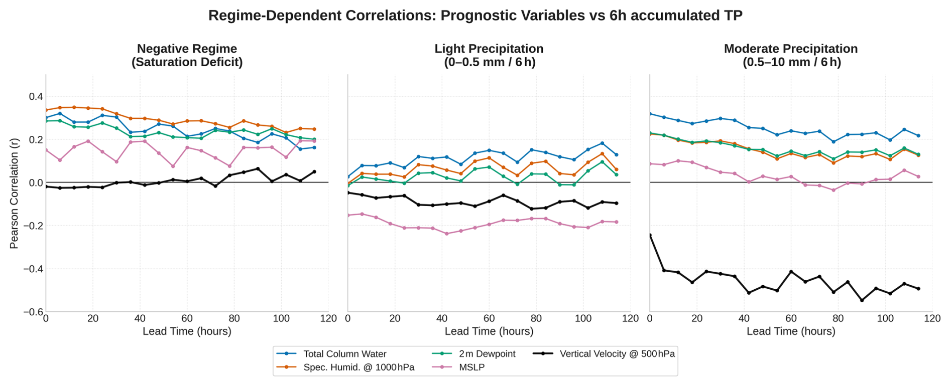
Figure 16 Regime-dependent correlations of pre-activation η (AIFS Revised), for a forecast issued the 1 June 2023 at 00:00 UTC. Pearson r between η and physical drivers across three regimes: negative space (η<0): high correlation with moisture variables (q₁₀₀₀, TCW) identifies η as a structured saturation deficit proxy (left panel). Light rain ($\mathrm{0}<\mathit{\eta }\le \mathrm{0.5}$ mm per 6 h): systematic weakening of correlation, likely associated with enhanced stochasticity in this regime (center panel). Moderate rain ($\mathrm{1}<\mathit{\eta }\le \mathrm{10}$ mm per 6 h): transition to dynamic control, with vertical velocity (w₅₀₀) as the dominant predictor ($r\approx -\mathrm{0.5}$) (right panel). Analysis covers a 120 h global forecast.

We computed the Pearson correlation coefficient (r) between the pre-activation field η and five key physical drivers: Total Column Water (TCW), Specific Humidity (q₁₀₀₀), 2 m Dewpoint (2d), Mean Sea Level Pressure (MSLP), and mid-tropospheric Vertical Velocity (w₅₀₀). As shown in Fig. 16, the results reveal a clear regime-dependent physical logic:

• Negative regime (η<0): we observe stable correlations (r≈0.3) with moisture variables (q₁₀₀₀, TCW, and 2d). This confirms that the negative space encodes a structured representation of the saturation deficit, kept physically consistent by gradients flowing from the prognostic moisture fields.

• Light precipitation ($\mathrm{0}<\mathit{\eta }\le \mathrm{0.5}$ mm): correlation with specific humidity, 2m dewpoint and total column water is substantially reduced in this regime. The weaker relationships are consistent with a lower signal-to-noise ratio and increased sensitivity to small-scale or non-linear processes.

• Moderate precipitation ($\mathrm{1}<\mathit{\eta }\le \mathrm{10}$ mm): the model transitions to dynamic control. While moisture correlations remain moderate, Vertical Velocity (w₅₀₀) emerges as the primary physical driver ($r\approx -\mathrm{0.5}$), illustrating the model's reliance on large-scale ascent to produce deterministic rainfall.

While presented as a targeted demonstration of internal model behaviour, the consistency of these signals across lead times suggests that this regime-specific transition is a fundamental structural property of the AIFS architecture. These results demonstrate that the negative pre-activation field encodes valuable information regarding a proxy for saturation deficit. We acknowledge that these correlations are computed from a single 5 d forecast, which limits the temporal sampling. However, the analysis is performed on a Gaussian reduced N320 grid, such that each 6-hourly forecast field contains more than 500 000 spatial evaluation points. Although based on one forecast initialization, the large number of grid-point samples per lead time provides a substantial statistical basis for examining the internal behaviour of the model.

4.1.2 Optimization geometry at the zero-precipitation boundary

Having established that the negative pre-activation space encodes physically meaningful information, we now turn to understanding why constraining it during training improves forecast skill for light precipitation. The mechanism can be understood by examining how the Mean Squared Error (MSE) interacts with model outputs in the vicinity of the zero-precipitation boundary for a non-bounded model:

1. Scenario A (Non-physical negative dry prediction): the model predicts a non-physical negative value ($\mathrm{tp}=-\mathrm{0.2}$ mm) for a dry observation (tp_obs=0 mm). The gradient of the Mean Squared Error (MSE) is:

   $$\begin{array}{}\text{(7)}& {\displaystyle \frac{\partial \mathcal{L}}{\partial \mathrm{tp}}}=\mathrm{2}\left(\mathrm{tp}-{\mathrm{tp}}_{\mathrm{obs}}\right)=\mathrm{2}(-\mathrm{0.2}-\mathrm{0})=-\mathrm{0.4}\left(\mathrm{Push}\mathrm{Up}\right).\end{array}$$

2. Scenario B (Underprediction): the truth is light rain (tp_obs=0.45 mm), but the model under-predicts the intensity (tp=0.25 mm). The gradient is:

   $$\begin{array}{}\text{(8)}& {\displaystyle \frac{\partial \mathcal{L}}{\partial \mathrm{tp}}}=\mathrm{2}(\mathrm{0.25}-\mathrm{0.45})=-\mathrm{0.4}\left(\mathrm{Push}\mathrm{Up}\right).\end{array}$$

3. Scenario C (Overprediction): the truth is dry or very light rain (tp_obs=0.05 mm), but the model over-predicts the intensity (tp=0.25 mm). The gradient is:

   $$\begin{array}{}\text{(9)}& {\displaystyle \frac{\partial \mathcal{L}}{\partial \mathrm{tp}}}=\mathrm{2}(\mathrm{0.25}-\mathrm{0.05})=+\mathrm{0.4}\left(\mathrm{Push}\mathrm{Down}\right).\end{array}$$

Because non-physical negative dry predictions (Scenario A) and genuine drizzle underpredictions (Scenario B) produce identical upward gradients, the optimizer receives an ambiguous training signal in the vicinity of zero. The loss provides no information about why the correction is required – whether it reflects a physical regime transition (dry → drizzle) or merely a violation of the non-negativity constraint. One might expect the model to self-organize by learning to place dry predictions in a compact negative range – say, around −0.1 mm – thereby avoiding interference with the light-rain regime. However, this equilibrium is dynamically unstable under MSE. A dry prediction at −0.1 mm receives the same upward gradient as a genuine drizzle underprediction, so stochastic gradient updates continually push dry samples toward and across zero. As a result, no stable attractor can form in the negative space.

Importantly, the instability is locally asymmetric around tp=0. For small tp=ϵ with $\mathit{ϵ}|\ll \mathrm{1}$),

$${\displaystyle \frac{\partial \mathcal{L}}{\partial \mathrm{tp}}}=\mathrm{2}\left(\mathit{ϵ}-{\mathrm{tp}}_{\mathrm{obs}}\right).$$

In the neighbourhood of zero, the target distribution is one-sided: tp_obs≥0, with strictly positive drizzle values arbitrarily close to zero but no negative observations. Let

$$\mathit{\mu }=\mathbb{E}\left[{\mathrm{tp}}_{\mathrm{obs}}\mid {\mathrm{tp}}_{\mathrm{obs}}\approx \mathrm{0}\right],\mathrm{with}\mathit{\mu }>\mathrm{0}.$$

Then

$$\mathbb{E}\left[{\displaystyle \frac{\partial \mathcal{L}}{\partial \mathrm{tp}}}\right]=\mathrm{2}(\mathit{ϵ}-\mathit{\mu }).$$

Hence the expected gradient is negative for all ϵ<μ, including the negative space. The only stationary point of the expected dynamics is $\mathit{ϵ}=\mathit{\mu }>\mathrm{0}$, which lies strictly on the positive side. Zero is therefore not a locally stable fixed point under MSE; stochastic gradient updates induce a systematic drift that transports dry predictions across the boundary into weakly positive values.

As a consequence, dry predictions do not concentrate at a stable negative value but instead occupy a diffuse region centered on zero, extending into both the negative and weakly positive ranges. The interval just above zero therefore contains a superposition of displaced dry cases and genuine drizzle events. This overlap reduces representational separability and compresses the effective dynamic range available to encode variability within the light-precipitation regime.

By enforcing non-negativity through a ReLU constraint during training, negative pre-activations are projected to zero before loss evaluation. As a result, dry samples no longer generate corrective gradients within the negative space. Zero becomes a hard boundary rather than a distributional equilibrium, and the dry regime collapses deterministically onto this boundary point. The positive axis is therefore freed to encode light-rain variability without contamination from non-physical corrective gradients.

Figure 17 allows the gradient-ambiguity argument to be verified quantitatively. The three panels form a closed chain of evidence. The non-bounded model produces dry or negative outputs at only ∼10 % of grid points, compared to ∼30 % for the bounded model. The top-right panel shows that the non-bounded model's light-precipitation frequency is inflated by almost exactly the same ∼20 percentage points. The non-bounded model is not detecting more drizzle; it is misclassifying displaced dry events as light rain. The bottom panel reveals the mechanism predicted by the expected-gradient analysis. The non-bounded model produces a narrow spike of density straddling zero, within which the dry and drizzle regimes are superimposed and statistically indistinguishable. The distribution is tightly concentrated near zero but exhibits a slight positive skew, consistent with the theoretical result that the local stationary point of the expected MSE gradient lies at a strictly positive value. In other words, the model attempts to encode dry states in the neighbourhood of zero, yet the systematic upward drift induced by $\mathbb{E}[\partial \mathcal{L}/\partial \mathrm{tp}]<\mathrm{0}$ for tp<μ prevents zero from acting as a stable attractor. The consequence is a persistent displacement of dry samples into weakly positive values, producing the observed excess of light precipitation.

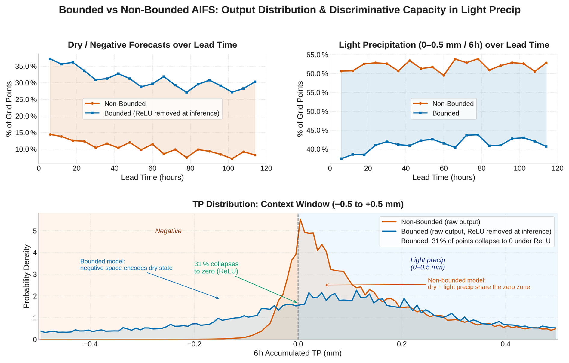
Figure 17 Output distribution and discriminative capacity in the light-precipitation regime for bounded and non-bounded AIFS. The bounded model's ReLU is removed at inference to expose raw pre-activations. Top left panel: the non-bounded model produces dry or negative outputs at only ∼10 % of grid points versus ∼30 % for the bounded model. A persistent 20-percentage-point gap across all lead times. Top right panel: the non-bounded model assigns ∼60 % of grid points to the light-precipitation bin (0–0.5 mm per 6 h) versus ∼40 % for the bounded model, an excess whose magnitude mirrors the dry-detection deficit almost exactly. Bottom panel: pre-activation density near zero. The non-bounded model concentrates dry and drizzle cases in an indistinguishable spike around zero; the bounded model distributes dry-state density broadly across the negative space, with 31 % of pre-activations collapsing cleanly to zero under ReLU at inference.

Although Fig. 17 illustrates a single 5 d forecast, the behavior is systematic rather than case-specific. This interpretation is reinforced by the Frequency Bias Index (FBI) and Peirce Skill Score (PSS) shown in Fig. 3 of the main article. The non-bounded configuration exhibits a pronounced positive frequency bias in the light-precipitation category, together with degraded discrimination skill, consistent with systematic misclassification of dry grid points as drizzle.

The mechanism described here provides a refined interpretation of recent findings in AI-driven precipitation forecasting. Sha et al. (2025a) reported that drizzle bias is substantially reduced when physical constraints are applied, whereas terrain-following coordinates alone do not mitigate drizzle bias but instead improve extreme precipitation forecasts. Notably, their constraint framework combines global conservation principles with an explicit non-negativity correction.

The present analysis isolates the role of non-negativity enforcement and demonstrates that it addresses a fundamental gradient asymmetry at the zero-precipitation boundary. This mechanism operates at the level of local optimization dynamics and provides a distinct, mechanistically interpretable pathway for drizzle reduction. While Sha et al. (2025a) demonstrate effectiveness of combining non-negativity with global conservation constraints, our analysis suggests that non-negativity merits investigation as an independent design element. The relative contributions of boundary enforcement versus conservation-based regularization, and their potential architecture dependence, remain important questions for future work.

4.2 Case studies

Headline verification scores for the revised AIFS show significant improvements over the conventional numerical weather prediction model. However, building trust in AI forecasting requires more than strong overall metrics. Forecasters place great importance on the ability of the model to accurately and reliably predict weather phenomena. They also value physically plausible outputs and recognizable weather patterns. To support this, we show below selected case studies.

4.2.1 Storm Éowyn

Storm Éowyn was an unusually strong winter storm and blizzard, initially impacting much of the Gulf Coast of the United States between 20 and 22 January 2025. This storm broke snowfall records at a number of reporting stations (Thiem and Collins, 2025) and represented an extreme out-of-training-distribution event with no clear analogies in the ERA5 reanalysis or the IFS Operational analysis dataset.

Figure 18 shows the AIFS and IFS forecasts at decreasing lead times for the affected area versus the corresponding IFS short-range forecast. The AIFS delivers an accurate forecast of snowfall for this extremely rare event. This showcases the ability of the model to accurately interpret meteorological patterns and forecast physically plausible events, even if they are far from the training data. The AIFS predicted the event with a lead time of 10 d, earlier than the IFS.

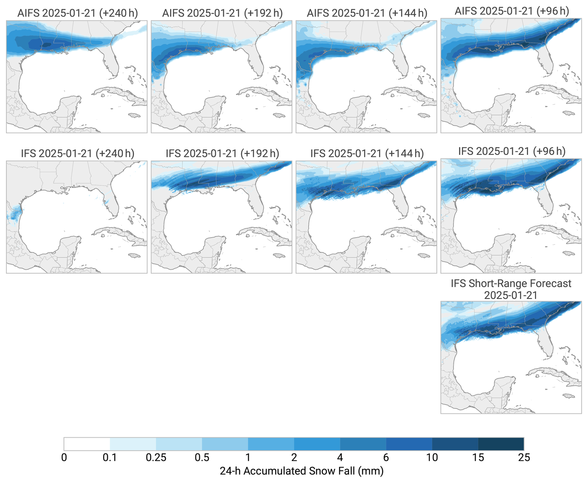
Figure 18 Snowfall forecasts for AIFS (top row panels) and IFS (middle row panels) over the Gulf Coast of America at 10, 8, 6 and 4 d lead times from left to right respectively, against IFS short-range forecasts for the snowfall event (bottom row panels). The figure shows how the snowfall event was forecast accurately 4 d ahead by both the IFS and AIFS. The AIFS forecasted the event even 10 d ahead.

4.2.2 Tropical low and extreme precipitation totals in Queensland Australia

Starting in late January 2025, a slow-moving summer storm brought exceptional rainfall along the northeastern coast of Queensland, Australia. Within a week, rainfall accumulation totalled more than 1000 mm in some areas, according to the Bureau of Meteorology as reported in NASA Earth Observatory (2025). The city of Townsville saw the equivalent of six months of rain in just 3 d and the largest weekly rainfall total was measured at a gauge in the Cardwell Range, southwest of Tully, where nearly 1700 mmfell (NASA Earth Observatory, 2025, Bureau of Meteorology measurements). Figure 19 compares forecasts from AIFS and IFS against the IMERG (Huffman et al., 2023) final product for the period 1–3 February 2025. Both model forecasts were initialized on 30 January 2025, 2 d prior to the event. The Cardwell Range is indicated by a black star, and the city of Townsville by a cyan star. Both IFS and AIFS successfully captured the event, with 24 h rainfall accumulations exceeding 300 mm in some regions. However, the AIFS forecast exhibits a somewhat persistent signal in the 5 d lead time, predicting very high rainfall totals near the Cardwell Range. This highlights that, despite AIFS's tendency toward excessive spatial smoothing, it remains capable of accurately forecasting extreme events at medium range.

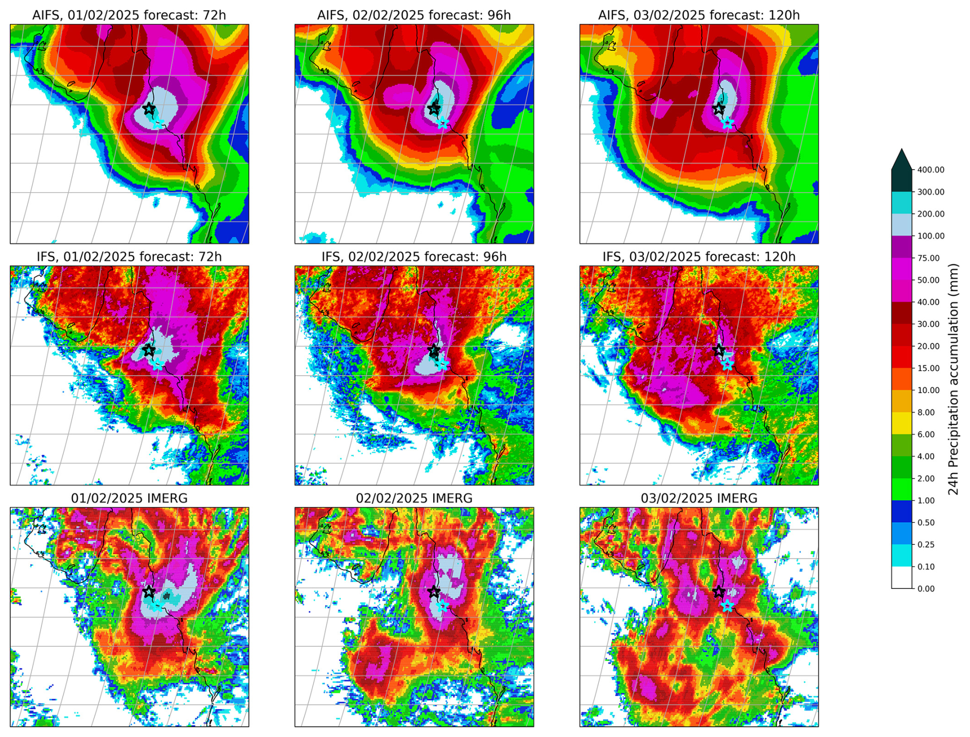
Figure 19 24 h accumulated precipitation forecasts from the AIFS (top row panels) and IFS (middle row) models, compared with IMERG observational data (bottom row panels) over northeastern Queensland for 1 to 3 February 2025. Forecasts are initialised on 30 January 2025. The black star marks the Cardwell Range, where rainfall totals exceeded 1600 mm over the week, and the cyan star marks the city of Townsville. Both models captured the core of the extreme rainfall event, with accumulations exceeding 300 mm in 24 h in some areas.

5 Discussion and conclusion

The revised AIFS version (1.1.0) presented here improves upon the pre-operational release through a revised training regime with more data, new forecast variables, improved stratospheric loss weights, and a bounding strategy that enforces physical constraints on the output variables. Overall, this leads to improvements of around 4 %–6 % across all variables, lead times, and pressure levels. The largest improvements, up to 12 % gains in normalized difference in the short range, are observed in total precipitation forecasting, which benefits from the newly introduced bounding. We showed that this has a significant impact on the prediction of no rain and light precipitation. The model displays good forecast performance for out-of-training-sample case studies, accurately capturing extreme precipitation and snowfall events.

Data plays a crucial role in the performance of AI models. Most of the improvements non-related to precipitation in the revised version of the AIFS stem from the expansion of the training dataset and the use of more recent operational ECMWF analyses for rollout fine-tuning, as demonstrated by the controlled comparison in Fig. 5. Since the AIFS relies on these analyses for real-time forecasting, it is important to fine-tune them regularly using up-to-date data. Regular fine-tuning with recent ECMWF analyses helps the models to adapt to shifts in the data due to new IFS model cycles.

Recent global AI forecasting systems, including GraphCast, Pangu-Weather, FuXi, and CREDIT, have reported persistent challenges in representing light precipitation. Positive frequency bias in the drizzle regime appears to be a recurring feature across models trained with symmetric regression losses on strictly non-negative, intermittent variables. Although these systems differ substantially in backbone architecture, from graph neural networks to transformer-based designs and modular physically constrained frameworks, the drizzle problem appears largely independent of architecture. Instead, it is closely tied to how precipitation is parameterized and constrained during training. Physical constraint methodologies offer multiple pathways for mitigating precipitation biases. Global conservation schemes may reduce drizzle indirectly by regulating total moisture budgets. The present analysis suggests that non-negativity enforcement addresses a more fundamental issue: the local gradient asymmetry at the zero boundary and the superposition of dry and wet states around zero. By introducing a hard geometric boundary at zero, the optimization landscape is reshaped such that dry and wet regimes become separable. This mechanism operates independently of large-scale conservation principles and may therefore represent a structural requirement for stable training of intermittent variables under MSE. Alternative activation functions such as LeakyReLU, which scale negative inputs by a small factor α (typically 0.01), would permit gradient flow in the negative space while heavily attenuating the loss contribution from dry predictions (by a factor of α²). We expect that similar regime separation would still emerge, since the cost of placing dry states deep in the negative space becomes negligible. The main practical difference is that LeakyReLU produces non-physical slightly negative output values at inference, requiring post-processing clipping. More broadly, alternative formulations that explicitly decouple the dry and wet regimes during training, such as asymmetric loss functions or dedicated classification heads for the no-rain state, represent promising directions for future work.

The bounding strategy presented here enforces physical realizability, non-negativity, boundedness, and inter-variable consistency, but does not impose global conservation of mass or energy. For the medium-range timescales considered in this work (up to 10 d), we expect conservation violations to remain small relative to forecast errors dominated by chaotic error growth, though a systematic quantification of mass and energy drift over extended AIFS integrations remains to be carried out.

Rollout fine-tuning emerges as an important factor shaping forecast behaviour, including the degree of spatial smoothing in the outputs. As the model is trained on extended lead times and optimised using a mean squared error objective, some degree of smoothing is expected. Training hyperparameters such as learning rate scheduling, number of optimisation steps, and rollout configuration can influence this behaviour and warrant further systematic investigation. In the present study, the training configuration, including a maximum rollout length of 12, was retained from the previous AIFS version to ensure consistency. The resulting Z500 power spectra (Fig. 6) are broadly comparable to those of the previous model across scales, including the ∼500 km range, with slightly improved agreement with the analysis at longer lead times. Importantly, these comparable spectral characteristics are achieved alongside overall improvements in RMSE-based skill (Fig. 7). This indicates that the skill gains are not obtained at the expense of degraded spatial variability. While more aggressive rollout strategies may further optimise headline verification scores, understanding their impact on spatial characteristics remains an important area for future work.

Alongside making updates to the training schedule, we have also added new variables to the AIFS while achieving improvements in forecast skill for headline atmospheric metrics. In particular, the inclusion of soil moisture and soil temperature as prognostic variables represents an initial step toward a more complete Earth system representation within AIFS. Targeted ablation studies are planned as the land-surface component is extended in future versions. However, it remains to be seen if adding more variables and earth-system components will eventually require an increase to the latent space of the model. The additional earth-system and energy-sector variables in AIFS establish a foundation for future extensions, including ocean and wave components, expanding the number of cryospheric processes with enhanced snow modelling, and increasing the hydrological capabilities of the model. These new variables are currently taken from a consistent data source with the rest of the model variables. In the future, there is the potential to look at datasets tailored to specific earth-system components, such as ERA5-Land (Muñoz Sabater et al., 2021) and the ocean and sea-ice reanalysis system (ORAS6) (Zuo et al., 2024).

AIFS currently operates at approximately 0.25° spatial resolution with a 6 h timestep, and future work will focus on increasing both spatial and temporal resolution.

The AIFS development has now transitioned to the new Anemoi framework (Lang et al., 2024a; Nipen et al., 2024; Wijnands et al., 2025). Anemoi provides tools for the whole data-driven modelling workflow, from the generation of training datasets, to scalable probabilistic training (Lang et al., 2024b) and running real-time inference with such models. Anemoi also allows for the cataloguing and archiving of model and data checkpoints to ensure reproducibility and traceability of training and inference runs and ensure that any models developed within this framework have a clear lineage. The Anemoi framework is now being used by an increasing number of Member States of ECMWF and collaborating organisations supported by ECMWF.

After a successful experimental phase, AIFS has transitioned to operational status at ECMWF on 25 February 2025. It is supported 24/7 alongside ECMWF's physics-based system, the IFS. The MSE trained model is labeled AIFS Single, and its forecasts are available earlier than the ones from the physics-based model chain, due to the fast runtime of AIFS.

Results presented in this paper show that AIFS forecasts are highly skilful and they outperform the IFS forecasts across the vast majority of lead times and variables. They highlight the relevance of AIFS for weather prediction. Future developments will focus on including more surface variables and exploring a wider range of applications such as climate reanalysis. The operational release of the AIFS demonstrates the commitment of ECMWF to pursue the best possible weather forecasts with both physics-based and machine learning methods.

Code and model availability.

• AIFS version 1.1.0 was fully trained using the Anemoi framework https://github.com/ecmwf/anemoi (last access: 31 March 2026). The frozen versions of the Anemoi modules used for training, together with the configuration files and the trained model checkpoint, are available in the permanent archive European Centre for Medium-Range Weather Forecasts (2025) under https://doi.org/10.5281/zenodo.17349820.

• The model weights for version 1.1.0 are also available on the project page on Hugging Face https://huggingface.co/ecmwf/aifs-single-1.1 (last access: 31 March 2026) under a Creative Commons Attribution 4.0 International (CC BY 4.0) licence and https://doi.org/10.57967/hf/6415 (ECMWF, 2025a).

• The AIFS Single model operational forecasts are freely available under ECMWF's Open Data Creative Commons licence (https://www.ecmwf.int/en/forecasts/datasets/open-data, last access: 31 March 2026) and https://doi.org/10.21957/open-data (ECMWF, 2025b) and forecast charts can be seen at https://charts.ecmwf.int/?query=aifs-single (last access: 31 March 2026).

• Further details on the model’s operationalization and data dissemination can be found at https://confluence.ecmwf.int/display/USS/OLD+-+Implementation+of+AIFS+Single+v1.0 (last access: 31 March 2026).