ForEdgeClim v1.0: a 3D process-based microclimate model incorporating vertical and lateral radiative and thermal fluxes to simulate forest edge-to-core transitions

Forest microclimates play a fundamental role in regulating biodiversity, ecosystem functioning, and forest resilience to climate change. However, most existing microclimate models focus on vertical processes and neglect lateral energy exchanges, limiting their ability to represent forest edge effects. Due to ongoing forest fragmentation, such lateral fluxes play an essential role in forest microclimate and associated ecological processes, particularly given that up to 20 % of global forest cover lies within 100 m of a forest edge.

Here, we introduce ForEdgeClim, a new process-based microclimate model implemented as a publicly available open-source R package that is able to simulate air and surface temperature at high spatial resolution along the forest edge-to-core continuum (here demonstrated at 1 m resolution). By explicitly leveraging high-resolution 3D forest structural data (e.g., derived from terrestrial laser scanning), the model represents a substantial advance over existing approaches that rely on simplified or spatially aggregated canopy descriptions. Building on this detailed structural representation, ForEdgeClim couples meteorological forcing with a physically based energy balance framework – including shortwave and longwave radiation, sensible and latent heat fluxes, and soil heat exchange – to simulate three-dimensional microclimate temperature patterns through a voxel-based radiative–thermal framework that explicitly represents vertical and lateral radiative and thermal exchanges, while representing wind-driven processes implicitly. Radiative transfer is represented using a two-stream approximation in both vertical and lateral directions, whereas the full energy balance is iteratively solved within a 3D voxel grid to account for coupled radiative and heat flux exchanges.

A Sobol sensitivity analysis indicates that heat-transfer processes dominate local air temperature dynamics (≥67 % of the total model output variance), whereas radiative transport plays a stronger role in controlling surface temperature and spatial temperature heterogeneity. These insights informed a targeted calibration of key model parameters. Model performance was evaluated using high-frequency in situ temperature measurements, with forest structural information derived from terrestrial laser scanning data, collected along a forest edge-to-core transect in a temperate forest in Belgium. Validation shows that ForEdgeClim successfully reproduces observed edge-to-core temperature gradients and fine-scale spatial variability in air temperature (R²≥0.87, RMSE≤2.01 °C).

By combining high-resolution structural information with a physically grounded yet computationally efficient framework, ForEdgeClim bridges the gap between simplified empirical microclimate models and computationally intensive ray-tracing approaches, which typically lack a full energy balance formulation. The model thus provides a versatile platform for microclimate research, ranging from biodiversity and habitat modelling to studies of forest-climate interactions under a changing environment, especially where edge effects play a key role in fragmented landscapes.

1 Introduction

Forest microclimates, defined as the fine-scale climatic conditions experienced within and beneath forest canopies, are key regulators of biodiversity, ecosystem functioning, and carbon cycling, as well as critical buffers of climate extremes (De Frenne et al., 2021). By moderating temperature and humidity conditions, forest microclimates shape species distributions and influence species' resilience to climate change (Sanczuk et al., 2023; Kemppinen et al., 2024). It is therefore essential to accurately represent forest microclimates for predicting ecosystem responses under future climate scenarios. Previous studies have shown that forest microclimate temperature can differ up to several degrees from free-air temperatures (De Frenne et al., 2019; Haesen et al., 2021; Ma et al., 2025; Zhou et al., 2025), and that these differences are strongly shaped by tree canopy structure and topography (Geiger et al., 1995; Jucker et al., 2018; Gao et al., 2021). Because microclimatic conditions are governed by the complex interplay among vegetation structure, radiation, and heat exchange processes operating across multiple spatial and temporal scales, modelling fine-scale (here, at 1 m resolution) thermal forest environments remains a major challenge (De Frenne et al., 2021).

Sub-canopy microclimates exhibit pronounced spatial variability over distances of only a few meters, reflecting fine-scale differences in canopy density, gap structure, and local terrain that characterise many structurally complex forest landscapes worldwide (Jucker et al., 2018). This spatial heterogeneity supports biodiversity by creating microhabitats and microrefugia and shaping recruitment niches for tree seedlings (Inman-Narahari et al., 2014; Scheffers et al., 2014; De Frenne et al., 2019; Soifer et al., 2025). A coarse-resolution or vertically aggregated model cannot resolve these fine-scale patterns. Hence, a high spatial resolution is essential for capturing ecologically relevant temperature variation throughout forest landscapes, including both interior and edge-influenced environments. Modelling frameworks that explicitly incorporate fine-scale variation in canopy structure are therefore better suited to provide realistic predictions of thermal environments below canopies. While such fine-scale heterogeneity also occurs within forest interiors, it is particularly pronounced near forest edges, where lateral radiative and convective fluxes interact with metre-scale variations in canopy structure. Recent studies using terrestrial laser scanning (TLS) in forests have shown that these edge environments induce persistent differences in tree architecture and allometric relationships, leading to additional ecosystem-level consequences such as reduced aboveground biomass (Nunes et al., 2023). However, other studies have reported higher carbon stocks at forest edges (Meeussen et al., 2021).

A wide range of modelling approaches has been developed to model microclimate, ranging from empirical downscaling techniques (Bramer et al., 2018; Haesen et al., 2023) to process-based energy balance models (Maclean, 2025), and biophysical species distribution models (Kearney and Porter, 2017; Kearney et al., 2021). While these models have advanced our understanding of local temperature dynamics, most treat energy fluxes in a vertically simplified manner and neglect lateral heat and radiation exchanges. This limitation particularly hampers the prediction of local temperatures near forest edges, where the edge itself, together with canopy gaps, allow for lateral light penetration and increased convective heat exchange (Chen et al., 1995; Malcolm, 1998; Davies-Colley et al., 2000; Dignan and Bren, 2003; De Pauw et al., 2022; Badouard et al., 2024). Accounting for lateral processes in forest edges are of particular importance due to forest fragmentation (Riitters et al., 2016; Zou et al., 2025). Haddad et al. (2015) estimated that nearly 20 % of global forest cover lies within 100 m of an edge, and this proportion exceeds 40 % in Europe (Estreguil et al., 2013). As a result, a substantial proportion of forests is influenced by edge effects that remain insufficiently represented in existing microclimate models.

Here, we present ForEdgeClim, a novel process-based modelling framework for simulating forest microclimate temperature gradients from edge to core. The model integrates high-resolution structural data (e.g., derived from TLS) with meteorological input data (atmospheric and soil temperatures and radiative fluxes) and a set of physically based energy balance components. ForEdgeClim explicitly represents both vertical and horizontal energy fluxes, including radiative transfer and heat exchange, resolved within a 3D voxel-based grid, with a primary focus on radiative and thermal processes while wind-driven processes are represented implicitly. By iteratively simulating these interacting processes, the framework predicts fine-scale spatial variability in microclimate temperature along gradients of forest structure and distance to forest edges. We apply ForEdgeClim to predict microclimate temperature conditions at 1 m resolution along a 135 m long edge-to-core transect in a European temperate forest. We evaluate the predictive performance of the model and identify the processes that most strongly shape edge-driven temperature gradients. To assess the model robustness and the influence of parameter uncertainty, we conducted a global sensitivity analysis, followed by parameter calibration and validation against empirical microclimate measurements. Together, these analyses provide a transparent assessment of ForEdgeClim and its suitability for studying microclimate gradients in structurally complex forests.

2 Model description

ForEdgeClim is a 3D, process-based microclimate model, implemented as an open-source R package (GitHub: https://github.com/qforestlab/ForEdgeClim (last access: 17 April 2026) and developed to simulate fine-scale temperature gradients along transects from the forest core towards the forest edge. The model operates on a spatially explicit voxel grid with a user-defined spatial resolution, here chosen as $\mathrm{1}\mathrm{m}\times \mathrm{1}\mathrm{m}\times \mathrm{1}\mathrm{m}$, in which each voxel represents a discrete three-dimensional volume of forest space. In this study, all simulations were performed at a spatial resolution of 1 m, selected as a compromise between resolving fine-scale structural heterogeneity and maintaining computational tractability. While the voxel resolution is configurable within the model framework, the effects of alternative spatial resolutions on model performance were not evaluated here and remain an important direction for future work. The model simulates microclimate conditions for individual time points based on meteorological input data, allowing the representation of instantaneous or (near) steady-state temperature patterns under specified atmospheric conditions.

This voxel-based, 3D formulation allows ForEdgeClim to directly integrate detailed 3D information on canopy and understorey structure – derived from terrestrial, mobile, or airborne sensing, or any comparable 3D data source – thereby linking structural heterogeneity to microclimatic variation. Each voxel contains a normalised density value between 0 and 1, which serves as a proxy for vegetation density and governs both radiative transfer and energy exchange. While vegetation within each voxel is treated as a bulk medium with uniform optical properties, structural heterogeneity at the canopy scale, including the presence of canopy gaps, is explicitly represented through the spatial configuration of voxel densities derived from TLS data. As a result, gap fraction variability and aspects of canopy clumping emerge from the three-dimensional arrangement of occupied and empty voxels, rather than being prescribed through explicit clumping indices or leaf area density profiles. The voxel-based 3D formulation enables the representation of vertical and lateral radiative and thermal energy fluxes, capturing key spatial interactions that characterise forest edge environments while parameterising turbulent and wind-driven processes implicitly. Details on high-resolution structural data processing and normalisation are provided in Sect. 3, and a detailed description of each model subprocess is presented in the subsequent sections of this paper.

Building on this spatial foundation, ForEdgeClim adopts a process-based, physically grounded framework based on the principle of energy conservation. Radiatively active environmental surfaces – including the semi-transparent canopy and the opaque forest floor – interact with both shortwave and longwave radiation through absorption, reflection, and, where applicable, transmission. These surfaces also emit thermal longwave radiation, exchange sensible heat with the surrounding air, and lose latent heat through evapotranspiration. The ground also acts as a temporary energy reservoir, storing and releasing heat, thereby contributing to the overall energy balance.

Each component of the energy budget depends explicitly on the local forest surface temperature (K), defined here as an effective surface temperature representing leaf and woody elements, weighted by their local structural density, through non-linear physical relationships. These include longwave radiation emission (Stefan–Boltzmann law), sensible heat exchange, and latent heat flux, all of which depend on the unknown surface temperature. As a result, the energy balance forms a coupled non-linear system within the voxel-based framework which is solved iteratively until convergence to a steady-state solution is achieved for a single moment in time. The iterative solution strategy represents a practical numerical approach for coupling multiple interacting voxel-scale energy exchange processes within the 3D framework.

Unlike bulk canopy approaches such as the Penman–Monteith formulation (Monteith, 1965), which represent the canopy as a spatially aggregated surface, ForEdgeClim resolves energy exchange at the scale of individual voxels within a three-dimensional forest structure derived from TLS data. In this spatially explicit representation, the energy balance must be solved separately for many surfaces with locally varying radiative and thermal conditions.

A schematic overview of the model workflow is presented in Fig. 1. Convergence is pursued for the forest surface temperature, while air and soil surface temperature (K) are updated diagnostically. The assumption of steady-state conditions is applied at the voxel scale, where local canopy and ground surfaces are assumed to reach thermal equilibrium much faster than the one-hour interval used in the simulations, allowing transient heat storage to be neglected. In the current model formulation, the energy balance is therefore solved independently for each simulated time point. For a given set of environmental forcing variables (e.g., macroclimate temperature, radiation, and soil temperature), the model iteratively converges to equilibrium conditions within the voxel grid. In this study, the model was applied using hourly meteorological forcing data, such that each time step represents a separate equilibrium solution. As a result, temporal heat storage and dynamic transitions between time steps are not explicitly simulated, and the model does not retain memory of previous states. Nevertheless, the model can be applied sequentially using time series of meteorological forcing data, allowing the reconstruction of temporally evolving microclimate patterns as a sequence of quasi-steady-state solutions. This formulation also enables coupling with ecological or vegetation models operating at hourly or daily time scales.

The model starts with simulating shortwave radiative transfer in two directions, vertical and lateral, using a two-dimensional radiative transfer module (SW RTM). It then iteratively closes the energy balance by minimising the residual energy (E_bal, W m⁻²) below a specified threshold, on the order of a few watts per square metre, depending on the spatial discretisation. This convergence criterion is consistent with commonly used thresholds in canopy energy balance models such as the SCOPE 2.0 model (Yang et al., 2021), where energy balance closure is achieved for residuals of approximately 1 W m⁻². Through successive updates, a stable and physically consistent temperature distribution is obtained. The balance equation is defined as:

$$\begin{array}{}\text{(1)}& R_{\mathrm{n}}-H-LE-G\le E_{\text{bal}},\end{array}$$

where R_n is the net radiation (W m⁻², including both shortwave and longwave components), H is the sensible heat flux (W m⁻²), LE is the latent heat flux (W m⁻²), and G is the ground heat flux (W m⁻²). The ground heat flux is set to zero for all voxels not in contact with the ground. Within the soil layer, G is used to compute the soil surface temperature (K), which, in turn, affects the air temperature (K). Sensible heat flux is calculated in three dimensions, while latent and ground heat fluxes are computed vertically.

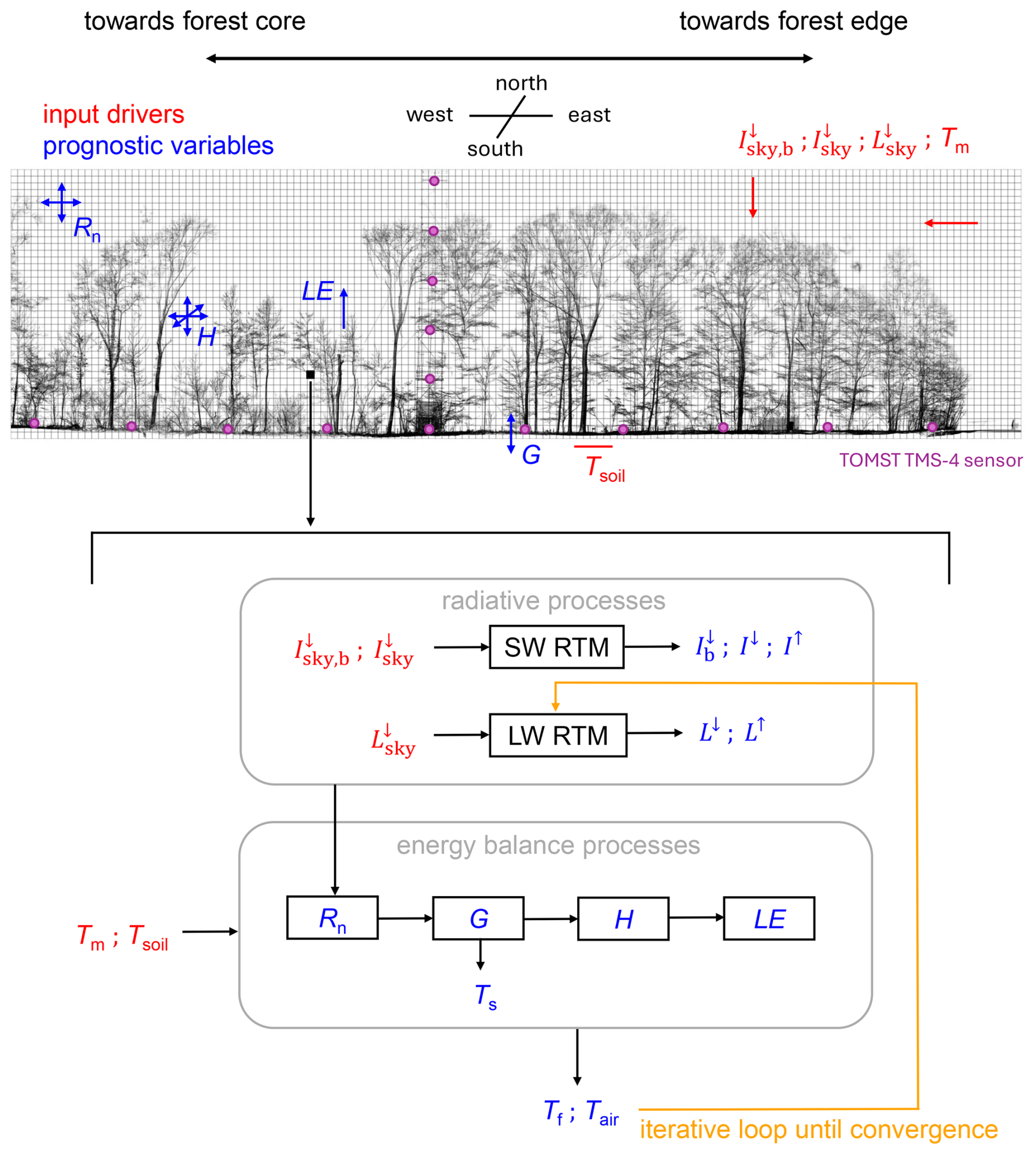
Figure 1 Conceptual overview of the ForEdgeClim modelling framework. Illustration of how a TLS-derived forest transect located in a temperate, deciduous forest in Belgium – from forest core to forest edge – serves as structural input for the model. Input drivers are shown in red and prognostic variables in blue. From a selected voxel within the transect, an arrow leads to a schematic representation of the ForEdgeClim workflow. In the transect figure, the four subprocesses – net radiation (R_n), sensible heat flux (H), latent heat flux (LE), and ground heat flux (G) – are shown with arrows indicating the spatial dimensions in which they operate. Given a latitude, longitude, date, hour, a 3D structural density grid, and initial values for the forest surface temperature (T_f; defined as an effective density-weighted temperature of leaf and woody element surfaces), air temperature (T_air), and soil surface temperature (T_s), ForEdgeClim uses the input drivers to iteratively run the subprocesses and determine the prognostic variables. Purple dots indicate the TOMST TMS-4 sensor positions, used for the calibration and validation of ForEdgeClim.
In the schematic, the subprocesses are placed in black boxes. $I_{\mathrm{b}}^{\downarrow }$, I^↓, and I^↑ respectively refer to the direct-beam, diffuse downward, and diffuse upward radiation, while L^↓ and L^↑ represent longwave downward and upward radiation. SW RTM and LW RTM indicate the shortwave and longwave radiative transfer models. $I_{\text{sky,b}}^{\downarrow }$, $I_{\text{sky}}^{\downarrow }$, and $L_{\text{sky}}^{\downarrow }$ correspond to the incoming direct-beam radiation, diffuse radiation, and longwave radiation at the forest boundary. T_m and T_soil denote the macrotemperature and soil temperature at the forest boundary.

2.1 Modelling temperatures

2.1.1 Forest surface temperature

ForEdgeClim models three temperature components. The first is the forest surface temperature (T_f, K), which represents an effective, density-weighted temperature of forest element surfaces within each voxel, including leaves, branches, and stems.

The model also simulates air temperature (T_air, K) and soil surface temperature (T_s, K). Air temperature relates to the individual voxels. As each voxel has a structural density value between 0 and 1, the remaining fraction (1 – density) represents the proportion of air. The soil surface temperature is treated as a single-layer value that characterises the ground surface temperature.

2.1.2 Air temperature

Air temperature is estimated through a linear interpolation approach similar to that used in the microclimate models microclimc (Maclean and Klinges, 2021) and its successor microclimf (Maclean, 2025), which simulate only vertical energy and radiation fluxes. In contrast, ForEdgeClim also resolves lateral fluxes:

$$\begin{array}{}\text{(2)}& T_{\text{air}}={\displaystyle \frac{(w_{\mathrm{m}X}+w_{\mathrm{m}Z})g_{\mathrm{m}}{T}_{\mathrm{m}}+w_{\mathrm{s}}{g}_{\mathrm{s}}{T}_{\mathrm{s}}+w_{\mathrm{f}}{g}_{\mathrm{f}}{T}_{\mathrm{f}}}{(w_{\mathrm{m}X}+w_{\mathrm{m}Z})g_{\mathrm{m}}+w_{\mathrm{s}}{g}_{\mathrm{s}}+w_{\mathrm{f}}{g}_{\mathrm{f}}}},\end{array}$$

where w represents a dimensionless weighting factor, g a convection coefficient ($\mathrm{W}{\mathrm{m}}^{-\mathrm{2}}{\mathrm{K}}^{-\mathrm{1}}$), and T a temperature (K). Subscripts m, s, and f refer to the macroenvironment, soil surface, and forest surface, respectively, while subscripts mX and mZ denote the lateral (x-axis) and vertical (z-axis) macroenvironmental boundaries.

In this formulation, air temperature is treated as a state variable defined on an Eulerian grid, with each voxel representing a fixed position in space. Heat exchange between neighbouring voxels and between air and surrounding surfaces is parameterised through effective exchange processes, which represent the net effect of turbulent mixing and small-scale air movement within the canopy. This approach is consistent with commonly used formulations in microclimate and canopy energy balance models (Campbell and Norman, 2000; Bonan, 2019), where turbulent transport is not explicitly resolved but represented through bulk exchange coefficients.

In this context, linearisation refers to approximating a non-linear relationship – typically between net energy balance and air temperature – by a local linear function. This allows the model to update air temperature using a simplified linear equation rather than repeatedly solving a full non-linear energy balance formulation, as is done for the forest surface temperature, making it computationally more efficient while still retaining high accuracy. Such linearised closures are commonly assumed to be appropriate when air–surface temperature differences remain small relative to the absolute temperature, such that higher-order non-linear terms can be neglected. These conditions are generally associated with sufficient air mixing, moderate radiation and humidity levels, and relatively homogeneous forest structures, under which turbulent transport can be reasonably approximated through bulk exchange processes.

In addition, vegetation density (ρ, dimensionless) directly scales the magnitude of surface–air energy exchange. In the model, ρ represents the effective fraction of vegetated surface within a voxel and enters explicitly in the formulations of sensible and latent heat fluxes (Eqs. 15 and 16). Voxels with higher density therefore exhibit stronger coupling between surface and air temperatures, whereas low-density voxels represent more open air space with reduced exchange.

The weights w are defined as exponentially decaying functions of the distance to a given boundary:

$$\begin{array}{}\text{(3)}& w_{\mathrm{s}}={\mathrm{e}}^{{\mathit{\alpha }}_{\mathrm{s}}{d}_{\mathrm{s}}}.\end{array}$$

Here, Eq. (3) shows the weighting for the soil surface (w_s), where d_s is the distance to the soil (m) and α_s is defined as:

$$\begin{array}{}\text{(4)}& {\mathit{\alpha }}_{\mathrm{s}}={\displaystyle \frac{\ln \left(\mathrm{0.5}\right)}{i_{\mathrm{s}}}},\end{array}$$

where the parameter i_s denotes the distance of influence (m), defined as the characteristic distance over which the effect of the soil surface temperature on air temperature decreases by 50 %. Exponential decay is appropriate for microclimate modelling, as it captures the gradual attenuation of influence with distance, maintains numerical stability, and reflects the physics of diffusive and convective heat transfer.

For voxels without structural elements (and therefore without a defined T_f), a virtual forest surface temperature is assigned by averaging the temperatures of the corresponding x-, y-, and z-plane surfaces.

The convection coefficients g and distances of influence i are prescribed model parameters treated as effective bulk exchange coefficients controlling the magnitude and spatial reach of heat exchange within the canopy. In the current model implementation, the coefficients g are prescribed as spatially uniform semi-empirical parameters and are not dynamically calculated from local wind speed, turbulence, or voxel-scale canopy structure. Instead, they represent characteristic canopy-scale exchange efficiencies under typical forest conditions. This effective parameterisation is commonly used in microclimate and canopy models where metre-scale turbulent transport and airflow dynamics cannot be explicitly resolved computationally (Campbell and Norman, 2000; Bonan, 2019). In this context, the coefficients g implicitly represent the combined effects of unresolved turbulent mixing, boundary-layer exchange, and small-scale convective heat transport within the canopy.

2.1.3 Soil surface temperature

The soil surface temperature is modelled using the one-dimensional heat conduction equation (i.e., Fourier's law):

$$\begin{array}{}\text{(5)}& T_{\mathrm{s}}=T_{\text{soil}}+{\displaystyle \frac{Gz}{k_{\mathrm{s}}}}.\end{array}$$

Here, T_soil (K) is the observed soil temperature at a reference depth. In our setup (see Sect. 3), this is measured at a depth of 8 cm at 20 locations within the forest transect. The variable z (m) represents the measurement depth (8 cm), G is the ground heat flux (W m⁻²), and k_s is the thermal conductivity of the soil ($\mathrm{W}{\mathrm{m}}^{-\mathrm{1}}{\mathrm{K}}^{-\mathrm{1}}$). The formulation represents conductive heat transfer between the soil surface and a shallow subsurface reference layer. This type of formulation is commonly used as a first-order approximation of ground heat exchange in models that do not explicitly resolve vertical soil heat transport (Campbell and Norman, 2000). The reference temperature T_soil varies over time following the measured soil temperature dynamics and is prescribed as a boundary condition. In the current implementation, k_s is treated as a constant parameter. In reality, soil thermal conductivity depends strongly on soil moisture content and soil composition, which are not explicitly represented in the model. As a result, spatial and temporal variability in soil thermal properties is not captured. The computation of G is described in Sect. 2.2.3.

2.2 Energy balance submodels

2.2.1 Radiative transfer model

Radiative processes are simulated in two dimensions (vertical and lateral) using a two-stream radiative transfer model (RTM) based on the formulation implemented in the ED2.2 model (Sellers, 1985; Oleson et al., 2013; Longo et al., 2019). A detailed description of the ForEdgeClim RTM can be found in Appendix A.

Briefly, the shortwave RTM simulates multi-scatter radiative transfer along a single column or row of voxels, where direct and diffuse sunlight interact with layered structures defined by voxel density (see Fig. A2 for a visualisation). Direct-beam radiation ($I_{\mathrm{b}}^{\downarrow }$, W m⁻²) follows an exponential decay:

$$\begin{array}{}\text{(6)}& {\displaystyle \frac{\mathrm{d}{I}_{\mathrm{b}}^{\downarrow }}{\mathrm{d}\mathit{\rho }}}=-K_{\mathrm{b}}{I}_{\mathrm{b}}^{\downarrow },\end{array}$$

while diffuse upward and downward components (I^↑, W m⁻²; I^↓, W m⁻²) are governed by the following coupled system of linear ordinary differential equations, which is subsequently discretised and solved as a linear system using a direct matrix solver based on LU decomposition:

$$\begin{array}{}\text{(7)}& {\displaystyle }& {\displaystyle }{\displaystyle \frac{\mathrm{d}{I}^{\downarrow }}{\mathrm{d}\mathit{\rho }}}={\displaystyle }-[\mathrm{1}-(\mathrm{1}-\mathit{\beta }\left)\mathit{\omega }\right]K_{\mathrm{d}}{I}^{\downarrow }+\mathit{\beta }\mathit{\omega }{K}_{\mathrm{d}}{I}^{\uparrow }+(\mathrm{1}-{\mathit{\beta }}_{\mathrm{0}})\mathit{\omega }{K}_{\mathrm{b}}{I}_{\mathrm{b}}^{\downarrow },\text{(8)}& {\displaystyle }& {\displaystyle \frac{\mathrm{d}{I}^{\uparrow }}{\mathrm{d}\mathit{\rho }}}=[\mathrm{1}-(\mathrm{1}-\mathit{\beta }\left)\mathit{\omega }\right]K_{\mathrm{d}}{I}^{\uparrow }-\mathit{\beta }\mathit{\omega }{K}_{\mathrm{d}}{I}^{\downarrow }-{\mathit{\beta }}_{\mathrm{0}}\mathit{\omega }{K}_{\mathrm{b}}{I}_{\mathrm{b}}^{\downarrow }.\end{array}$$

In these equations (derived as Eqs. A3 and A4 in Appendix A), dρ denotes the change in forest density with depth in canopy (dimensionless), ω the shortwave scattering coefficient (dimensionless), and β and β₀ the fractions of scattered diffuse and scattered direct-beam radiation in the backward direction (dimensionless). K_d and K_b are the diffuse and direct-beam extinction coefficients (dimensionless), respectively. All parameter definitions are given in Table 1. The two-stream formulations (Eqs. 6–8) are presented in their continuous form for clarity. In ForEdgeClim, however, they are solved in a discretised form across the voxel grid, using finite-difference updates of $I_{\mathrm{b}}^{\downarrow }$, I^↓, and I^↑ layer by layer along the radiative path.

Campbell and Norman (2000)Campbell and Norman (2000)Campbell and Norman (2000)Campbell and Norman (2000)Wiscombe and Grams (1976)Wiscombe and Grams (1976)Campbell and Norman (2000)Campbell and Norman (2000)Campbell and Norman (2000)Campbell and Norman (2000)Rotenberg et al. (1998)Rotenberg et al. (1998)Wiscombe and Grams (1976)Campbell and Norman (2000)Campbell and Norman (2000)Campbell and Norman (2000)Monteith and Unsworth (2013)Monteith and Unsworth (2013)Monteith and Unsworth (2013)De Pauw et al. (2024)Davies-Colley et al. (2000)Gao et al. (2021)Glocke et al. (2025)Monteith and Unsworth (2013)Campbell and Norman (2000)Monteith and Unsworth (2013)Yang et al. (2021)

Table 1 Model parameters related to the energy balance, radiative transfer, and heat exchange subprocesses in the ForEdgeClim framework. The column U(min, max) lists the minimum and maximum parameter values reported for, or inferred from, temperate forest studies, as documented in the literature sources listed in the references column. Within ForEdgeClim, each parameter is assigned a uniform distribution across this range, which serves as the prior distribution during the calibration procedure. The column submodel indicates the component of the model to which each parameter belongs. SW RTM refers to the shortwave radiative transfer model, LW RTM to the longwave radiative transfer model, H to the sensible heat flux, G to the ground heat flux, T_air to the calculation of air temperature, and T_s to the calculation of soil surface temperature. Parameters shown in boxes are those selected for calibration (see Sect. 5.2 for justification of parameter selection).

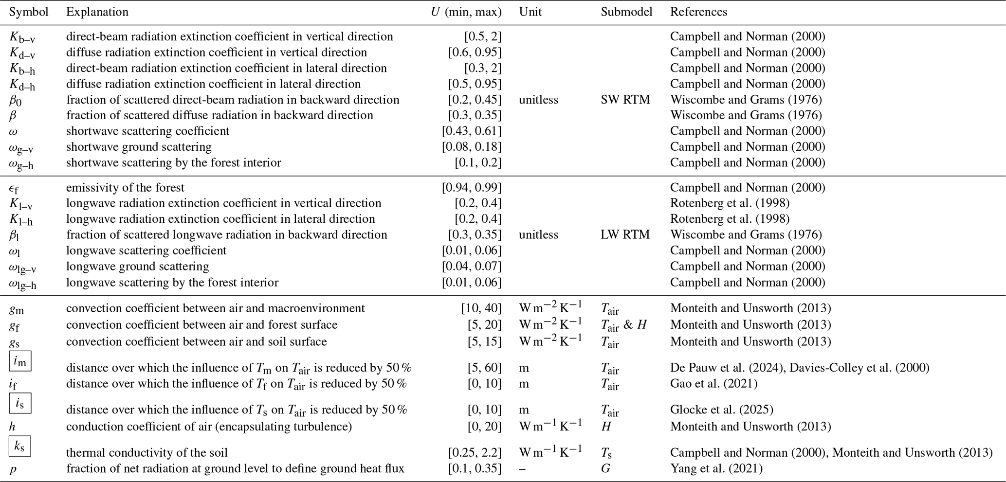
To build physical intuition for the extinction coefficients: in dense canopies, vertical direct-beam extinction coefficients (K_b) typically approach 0.9, reflecting strong attenuation by leaves and branches. Diffuse radiation is attenuated less strongly (K_d<K_b), as it arrives from multiple directions and can pass through canopy gaps. Lateral attenuation coefficients are generally smaller than vertical ones because radiation can travel longer path lengths through the canopy, a consequence of leaves typically being more horizontally inclined (Liu et al., 2019). Seasonal variability in attenuation can be represented by adjusting K_b and K_d to account for changes in leaf phenology.

The shortwave RTM is implemented as a one-dimensional column model. To obtain a two-dimensional radiative field, it is applied sequentially to each vertical column (fixed x and y) and each horizontal row (fixed y and z) in the 3D voxel grid. Direct-beam solar radiation is partitioned between the vertical and lateral directions according to the solar elevation angle, whereas diffuse radiation is assumed to be isotropic, such that vertically and laterally incident diffuse fluxes are equal.

This formulation represents the three-dimensional radiation field as a set of coupled one-dimensional vertical and lateral radiative transfer problems. While this introduces a simplified representation of the angular distribution of radiation, it enables the model to capture the dominant radiative gradients associated with vertical attenuation and lateral radiation penetration at forest edges in a computationally efficient manner. The radiative transfer scheme is therefore directionally resolved within the vertical and lateral domains, but does not explicitly discretise the full three-dimensional angular radiation field. Anisotropy is thus only partially represented through the separation of vertical and lateral fluxes and the dependence of direct radiation on solar elevation angle.

2.2.2 Net radiation

Net radiation (R_n) represents the net radiative energy available at a surface, resulting from the balance between incoming and outgoing shortwave and longwave radiation. It comprises three shortwave RTM components – direct-beam ($I_{\mathrm{b}}^{\downarrow }$), diffuse downward (I^↓), and diffuse upward (I^↑) – and two longwave RTM components – longwave downward (L^↓) and longwave upward (L^↑):

$$\begin{array}{}\text{(9)}& R_{\mathrm{n}}=I_{\mathrm{b}}^{\downarrow }+I^{\downarrow }-I^{\uparrow }+L^{\downarrow }-L^{\uparrow }.\end{array}$$

Longwave radiation is computed using an analogous two-stream formulation to that of the shortwave RTM, but without direct-beam terms and including thermal emission from forest surfaces. The longwave upward and downward components (L^↑, W m⁻²; L^↓, W m⁻²) are governed by the following coupled system of linear ordinary differential equations, which is subsequently discretised and solved as a linear system using a direct matrix solver:

$$\begin{array}{}\text{(10)}& {\displaystyle }& {\displaystyle \frac{\mathrm{d}{L}^{\downarrow }}{\mathrm{d}\mathit{\rho }}}=-[\mathrm{1}-(\mathrm{1}-\mathit{\beta }\left)\mathit{\omega }\right]K_{\mathrm{l}}{L}^{\downarrow }+\mathit{\beta }\mathit{\omega }{K}_{\mathrm{l}}{L}^{\uparrow }+{\mathit{ϵ}}_{\mathrm{f}}\mathit{\sigma }{T}_{\mathrm{f}}^{\mathrm{4}}{K}_{\mathrm{l}},\text{(11)}& {\displaystyle }& {\displaystyle \frac{\mathrm{d}{L}^{\uparrow }}{\mathrm{d}\mathit{\rho }}}=[\mathrm{1}-(\mathrm{1}-\mathit{\beta }\left)\mathit{\omega }\right]K_{\mathrm{l}}{L}^{\uparrow }-\mathit{\beta }\mathit{\omega }{K}_{\mathrm{l}}{L}^{\downarrow }-{\mathit{ϵ}}_{\mathrm{f}}\mathit{\sigma }{T}_{\mathrm{f}}^{\mathrm{4}}{K}_{\mathrm{l}}.\end{array}$$

Here, K_l is the longwave extinction coefficient (dimensionless). The forest emissivity (ϵ_f, dimensionless) and Stefan–Boltzmann constant (σ, $\mathrm{W}{\mathrm{m}}^{-\mathrm{2}}{\mathrm{K}}^{-\mathrm{4}}$) define the emitted longwave flux. All model constants are given in the appendix, Table B1. As with the shortwave RTM, these longwave equations are numerically implemented in discretised form, with fluxes updated sequentially across voxels.

2.2.3 Ground heat flux

Ground heat flux (G) represents the transfer of energy between the ground surface and the underlying soil. It is modelled as a fixed proportion of the net radiation at the ground surface:

$$\begin{array}{}\text{(12)}& G=p(\mathrm{1}-\mathit{\rho })R_{\mathrm{n}},\end{array}$$

following the approach implemented in the SCOPE 2.0 model (Yang et al., 2021). Here, p is the fraction of R_n that is absorbed by the soil surface and ρ is the forest structural density of the voxel layer directly above the soil (dimensionless). Ground heat flux is therefore reduced under dense vegetation cover, where less radiation reaches the soil surface. Throughout this manuscript, ρ refers to voxel vegetation density (dimensionless), whereas ρ_air denotes air density (kg m⁻³).

Equation (12) provides a simplified local closure of the surface energy balance and implicitly assumes that ground heat flux responds instantaneously to net radiation. As such, the formulation does not explicitly resolve temporal phase shifts associated with heat storage and delayed conductive heat transport within deeper soil layers.

The resulting flux is used to estimate soil surface temperature (Sect. 2.1.3), which in turn influences near-surface air temperature (Sect. 2.1.2) and the overall energy balance.

2.2.4 Sensible heat flux

Sensible heat flux (H) represents the transfer of thermal energy between forest surfaces and the surrounding air. In ForEdgeClim, this process is simulated in three dimensions and includes two components: (i) heat exchange between adjacent air voxels:

$$\begin{array}{}\text{(13)}& {\displaystyle }& {\displaystyle }D=hA{\displaystyle \frac{\mathrm{\Delta }{T}_{\text{air}}}{\mathrm{\Delta }x}},\text{(14)}& {\displaystyle }& {\displaystyle }{T}_{\text{air,new}}=T_{\text{air,old}}-{\displaystyle \frac{D}{c_{\mathrm{p}}{\mathit{\rho }}_{\text{air}}V}},\end{array}$$

and (ii) heat exchange between forest elements and the air:

$$\begin{array}{}\text{(15)}& H=\mathit{\rho }{g}_{\mathrm{f}}(T_{\mathrm{f}}-T_{\text{air}}),\end{array}$$

where h ($\mathrm{W}{\mathrm{m}}^{-\mathrm{1}}{\mathrm{K}}^{-\mathrm{1}}$) is an effective heat transfer coefficient governing air–air exchange between adjacent voxels, and g_f ($\mathrm{W}{\mathrm{m}}^{-\mathrm{2}}{\mathrm{K}}^{-\mathrm{1}}$) is a bulk forest–air sensible heat transfer coefficient. Here, ρ represents the voxel-scale vegetation density (dimensionless), such that sensible heat exchange increases proportionally with the amount of vegetated surface present within a voxel.

Boundary conditions allow heat exchange with the macroenvironment at the canopy and forest edge, with the soil at the lower boundary, and impose a no-flux condition at the forest core.

In Eqs. (13)–(15), A is the surface area of one voxel face (m²), ΔT_air is the air temperature difference between adjacent voxels (K), Δx is the voxel size (m), T_air,new and T_air,old are the updated and previous air temperatures (K), c_p ($\mathrm{J}{\mathrm{kg}}^{-\mathrm{1}}{\mathrm{K}}^{-\mathrm{1}}$) is the specific heat capacity of air, ρ_air (kg m⁻³) is air density, V is the voxel volume (m³), and ρ is the voxel's forest structural normalised density (dimensionless).

The air–air heat exchange term (Eqs. 13 and 14) represents effective thermal transport driven by local temperature gradients. This parameterisation does not explicitly resolve the underlying transport processes, but instead captures their combined effect at the voxel scale through the coefficient h. In practice, heat transport is expected to be dominated by turbulent mixing under most conditions, while molecular diffusion contributes only marginally.

The forest–air heat exchange term (Eq. 15) represents the net sensible heat transfer between vegetation surfaces (e.g., leaves, branches, and stems) and the surrounding air. The coefficient g_f is treated as an effective bulk sensible heat exchange parameter representing the characteristic efficiency of heat transfer between vegetation surfaces and surrounding air under typical canopy conditions. It implicitly accounts for unresolved turbulent mixing, boundary-layer convection, and small-scale air movement within the canopy.

This formulation allows sensible heat fluxes to respond to local temperature gradients and forest structural density, while maintaining computational efficiency within the voxel-based framework.

2.2.5 Latent heat flux

Latent heat flux (LE) represents the transfer of energy associated with phase changes of water, including both evaporation and transpiration (i.e., evapotranspiration) from forest surfaces to the atmosphere. In ForEdgeClim, LE is estimated using the empirical Priestley–Taylor method:

$$\begin{array}{}\text{(16)}& LE=\mathit{\rho }\mathit{\alpha }{R}_{\mathrm{n}}{\displaystyle \frac{s\left(T_{\mathrm{f}}\right)}{s\left(T_{\mathrm{f}}\right)+\mathit{\gamma }}},\end{array}$$

which provides a simplified form of the Penman–Monteith equation by representing evapotranspiration as a function of available radiative energy (Lhomme, 1997). Here, ρ refers to voxel vegetation density (dimensionless), α (dimensionless) is the Priestley–Taylor coefficient, γ is the psychrometric constant (kPa K⁻¹), and s(T_f) is the slope of the saturation vapour pressure curve.

In this formulation, evapotranspiration is represented as a bulk canopy flux. Stomatal regulation and canopy resistance are not explicitly resolved; instead, their combined effects, together with atmospheric controls, are implicitly captured in the empirical coefficient α. As a result, this approach provides a first-order approximation of latent heat flux under conditions where evapotranspiration is primarily energy-limited (Monteith and Unsworth, 2013). Consequently, the current formulation does not explicitly represent dynamic stomatal responses to environmental drivers such as vapour pressure deficit, soil moisture limitation, or drought stress. The latent heat flux formulation should therefore be interpreted as a simplified first-order approximation of canopy evapotranspiration.

The slope of the saturation vapour pressure curve is defined as:

$$\begin{array}{}\text{(17)}& s\left(T_{\mathrm{f}}\right)=\mathrm{4098}{\displaystyle \frac{e_{\mathrm{s}}\left(T_{\mathrm{f}}\right)}{(T_{\mathrm{f}}-\mathrm{35.85}{)}^{\mathrm{2}}}}.\end{array}$$

The saturation vapour pressure e_s(T_f) is estimated using the empirical formulation of Tetens:

$$\begin{array}{}\text{(18)}& e_{\mathrm{s}}\left(T_{\mathrm{f}}\right)=\mathrm{0.6108}\cdot \exp \left({\displaystyle \frac{\mathrm{17.27}(T_{\mathrm{f}}-\mathrm{273.15})}{T_{\mathrm{f}}-\mathrm{35.85}}}\right),\end{array}$$

which provides a reliable approximation of the Clausius–Clapeyron relationship for temperatures up to 50 °C (Anyadike, 1984).

2.3 Solving the energy balance

Within each iteration, the energy balance is solved simultaneously for all voxels, and iterations are repeated until convergence is reached for the entire system. During each iteration, the components of the energy budget – net radiation, sensible heat flux, latent heat flux, ground heat flux, air temperature, and soil surface temperature – are updated according to the newly estimated forest surface temperature.

Similar to the approach of the SCOPE 2.0 model (Yang et al., 2021), Newton's method is applied to update surface temperature values between successive iteration steps. This method iteratively drives the energy balance closure error (E_bal) towards zero by adjusting the forest surface temperature (T_f), using the derivative of the error with respect to T_f:

$$\begin{array}{}\text{(19)}& T_{\text{f,new}}=T_{\text{f,old}}-W{\displaystyle \frac{E_{\text{bal}}\left(T_{\mathrm{f}}\right)}{\frac{\mathrm{d}{E}_{\text{bal}}\left(T_{\mathrm{f}}\right)}{\mathrm{d}{T}_{\mathrm{f}}}}}.\end{array}$$

Here, W is a damping factor applied to the Newton update of forest surface temperature to improve numerical stability and prevent oscillations. W is initialised at 1 and adaptively reduced when the maximum absolute energy-balance residual across all voxels increases between iterations, down to a minimum value of 0.01.

From Eq. (1), the derivative of the energy balance error with respect to T_f can be expressed as:

$$\begin{array}{}\text{(20)}& {\displaystyle \frac{\mathrm{d}{E}_{\text{bal}}\left(T_{\mathrm{f}}\right)}{\mathrm{d}{T}_{\mathrm{f}}}}={\displaystyle \frac{\mathrm{d}{R}_{\mathrm{n}}\left(T_{\mathrm{f}}\right)}{\mathrm{d}{T}_{\mathrm{f}}}}-{\displaystyle \frac{\mathrm{d}H\left(T_{\mathrm{f}}\right)}{\mathrm{d}{T}_{\mathrm{f}}}}-{\displaystyle \frac{\mathrm{d}LE\left(T_{\mathrm{f}}\right)}{\mathrm{d}{T}_{\mathrm{f}}}}.\end{array}$$

Note that the derivative of G is omitted, as the ground heat flux is computed only for the soil surface temperature and not for the forest surface temperature. Consequently, G is independent (to first order) of T_f. Combining Eq. (20) with Eqs. (9), (15), and (16) leads to:

$$\begin{array}{}\text{(21)}& \begin{array}{rl}{\displaystyle \frac{\mathrm{d}{E}_{\text{bal}}\left(T_{\mathrm{f}}\right)}{\mathrm{d}{T}_{\mathrm{f}}}}& {\displaystyle }=-\mathrm{4}{\mathit{ϵ}}_{\mathrm{f}}\mathit{\sigma }{T}_{\mathrm{f}}^{\mathrm{3}}-\mathit{\rho }{g}_{\mathrm{f}}-\mathit{\rho }\mathit{\alpha }\left(-\mathrm{4}{\mathit{ϵ}}_{\mathrm{f}}\mathit{\sigma }{T}_{\mathrm{f}}^{\mathrm{3}}\right)\\ {\displaystyle }& {\displaystyle }\times {\displaystyle \frac{s\left(T_{\mathrm{f}}\right)}{s\left(T_{\mathrm{f}}\right)+\mathit{\gamma }}}+\mathit{\rho }\mathit{\alpha }{R}_{\mathrm{n}}{\displaystyle \frac{\mathrm{d}F\left(T_{\mathrm{f}}\right)}{\mathrm{d}{T}_{\mathrm{f}}}},\end{array}\end{array}$$

where F(T_f) is further defined as:

$$F\left(T_{\mathrm{f}}\right)={\displaystyle \frac{s\left(T_{\mathrm{f}}\right)}{s\left(T_{\mathrm{f}}\right)+\mathit{\gamma }}},$$

and thus, its derivative is given by:

$$\begin{array}{ll}{\displaystyle \frac{\mathrm{d}F\left(T_f\right)}{\mathrm{d}{T}_{\mathrm{f}}}}& {\displaystyle }={\displaystyle \frac{\frac{\mathrm{d}s\left(T_{\mathrm{f}}\right)}{\mathrm{d}{T}_{\mathrm{f}}}(s+\mathit{\gamma })-s\frac{\mathrm{d}s\left(T_{\mathrm{f}}\right)}{\mathrm{d}{T}_{\mathrm{f}}}}{(s+\mathit{\gamma }{)}^{\mathrm{2}}}}\\ {\displaystyle }& {\displaystyle }={\displaystyle \frac{\mathit{\gamma }\frac{\mathrm{d}s\left(T_{\mathrm{f}}\right)}{\mathrm{d}{T}_{\mathrm{f}}}}{(s+\mathit{\gamma }{)}^{\mathrm{2}}}},\end{array}$$

with

$$\begin{array}{rl}{\displaystyle }& {\displaystyle \frac{\mathrm{d}s\left(T_{\mathrm{f}}\right)}{\mathrm{d}{T}_{\mathrm{f}}}}=\\ {\displaystyle }& {\displaystyle }{\displaystyle \frac{\mathrm{4098}\frac{\mathrm{d}{e}_{\mathrm{s}}\left(T_{\mathrm{f}}\right)}{\mathrm{d}{T}_{\mathrm{f}}}(T_{\mathrm{f}}-\mathrm{35.85}{)}^{\mathrm{2}}-\mathrm{2}(T_{\mathrm{f}}-\mathrm{35.85}\left)\mathrm{4098}{e}_{\mathrm{s}}\right(T_{\mathrm{f}})}{(T_{\mathrm{f}}-\mathrm{35.85}{)}^{\mathrm{4}}}},\end{array}$$

and

$$\begin{array}{rl}{\displaystyle \frac{\mathrm{d}{e}_{\mathrm{s}}\left(T_{\mathrm{f}}\right)}{\mathrm{d}{T}_{\mathrm{f}}}}& {\displaystyle }=\mathrm{0.6108}\cdot \exp \left({\displaystyle \frac{\mathrm{17.27}(T_{\mathrm{f}}-\mathrm{273.15})}{T_{\mathrm{f}}-\mathrm{35.85}}}\right)\\ {\displaystyle }& {\displaystyle }\times {\displaystyle \frac{(T_{\mathrm{f}}-\mathrm{35.85})\mathrm{17.27}-\mathrm{17.27}(T_{\mathrm{f}}-\mathrm{273.15})}{(T_{\mathrm{f}}-\mathrm{35.85}{)}^{\mathrm{2}}}}.\end{array}$$

This formulation enables temperature-dependent feedback between radiation, heat exchange, and evapotranspiration, while promoting stable and robust convergence towards a physically consistent energy balance at each iteration. Numerical stability is enhanced through the use of a damped Newton scheme with adaptive step-size control. A supporting figure illustrating typical convergence behaviour for representative voxels is provided in the appendix, Fig. C1.

2.4 Numerical implementation

ForEdgeClim employs a grid-based numerical framework to simulate microclimate temperature and energy exchange in fragmented forests. The 3D voxel representation enables spatially explicit calculations and efficient computation of radiative and heat-transfer processes.

The model combines two numerical methods: the finite difference method (FDM) and the finite volume method (FVM). The FDM is used to simulate air-to-air conductive heat transfer within the sensible heat flux submodel (Fourier's law), where temperature gradients are approximated using finite-difference schemes. It is also used to solve the shortwave and longwave radiative transfer models (RTMs), in which the continuous two-stream differential equations are discretised and evaluated layer by layer along the radiative path. Upward and downward fluxes are updated sequentially using explicit finite-difference stepping, allowing radiation to be absorbed, scattered, and transmitted as it propagates through the 3D voxel grid. The FVM is applied to solve the energy balance equation, ensuring conservation of energy fluxes at the voxel scale. This combination allows both accurate representation of local heat diffusion and energy conservation across adjacent voxels.

The model operates on a 3D voxel grid. Although a voxel size of 1 m³ was adopted in this study to match the TLS-derived structural data, the voxel resolution is a configurable model constant and can be freely adjusted, subject to the spatial resolution and information content of the input structural data. ForEdgeClim can therefore be run at coarser or finer spatial resolutions (e.g., $\mathrm{2}\mathrm{m}\times \mathrm{2}\mathrm{m}\times \mathrm{2}\mathrm{m}$) depending on the desired level of structural detail, and computational constraints.

For the voxel resolution used here (1 m³), a single model run for one hourly time point required between 20 s and two minutes of computation on a Dell laptop equipped with an Intel^® Core™ i7-13800H processor (2.50 GHz) and 32 GB RAM running a 64-bit operating system. These simulations were performed on a voxel grid of $\mathrm{135}\mathrm{m}\times \mathrm{30}\mathrm{m}\times \mathrm{38}\mathrm{m}$ (edge-to-core length × width × canopy height). The computational cost scales approximately linearly with the total number of voxels in the domain, and thus depends on both spatial resolution and domain size, as most calculations are performed locally within or between neighbouring voxels. For such a run, the energy balance error was constrained to less than 2 W m⁻², which typically required between 7 and 10 iterations to achieve convergence (see Fig. C1).

A structured voxel-based discretisation was adopted because it aligns naturally with voxelised forest representations derived from TLS point cloud data (Hosoi et al., 2013) and enables efficient numerical coupling of radiative transfer, heat exchange, and evapotranspiration processes. The use of structured grids facilitates the application of finite-difference and finite-volume schemes and allows energy fluxes to be consistently exchanged between adjacent voxels within a unified numerical framework.

3 Study site and observational data

We applied ForEdgeClim on the Aelmoeseneiebos, a temperate deciduous forest in Gontrode, Belgium (50.980° N, 3.816° E). A 135 m×30 m east–west oriented transect was established from the forest edge into the core, spanning stands dominated by pedunculate oak (Quercus robur) and European beech (Fagus sylvatica) in the east and European ash (Fraxinus excelsior) and sycamore (Acer pseudoplatanus) in the west. The transect consisted of three parallel measurement lines (central, northern, and southern), spaced 15 m apart, together covering the full 30 m transect width. Along the central line, 10 TOMST TMS-4 loggers (TOMST Ltd., Prague, Czech Republic), with a manufacturer-specified accuracy of ±0.5 °C over the range −40 to 60 °C (Wild et al., 2019), were installed at 15 m intervals. These loggers measured air temperature at 15 cm above ground and soil temperature at 8 cm depth (purple dots positioned on the ground in Fig. 1). On both the northern and southern lines, five such sensors were placed at 30 m intervals. In addition, a meteorological tower is positioned approximately at the centre of the transect (75 m from the eastern edge) with five vertically distributed TOMST TMS-4 sensors installed every 7 m to capture a vertical temperature profile (purple dots positioned on the tower in Fig. 1). All TOMST TMS-4 sensors were used from July 2023–April 2025, recording at 15 min intervals. The establishment of the transect is also explained in Sanczuk et al. (2025).

3D structural forest data were collected monthly, also from July 2023–April 2025, using a RIEGL VZ400i terrestrial laser scanner (RIEGL Laser Measurement Systems GmbH, Horn, Austria) at 15 m intervals along the transect lines, coinciding with the TOMST TMS-4 sensor locations. The instrument operates at a wavelength of 1550 nm and has a nominal beam divergence of 0.35 mrad. It covers a full azimuthal range of 0–360° and a zenith angle range of 30–130°. Scans were conducted with an angular resolution of 0.04° in both azimuth and zenith, using a pulse repetition frequency of 600 kHz. At each location, two scans were conducted – a vertical scan and a scan tilted 90° from vertical – to reduce canopy occlusion effects. The scans were filtered by retaining points with reflectance between −20 and 5 dB and deviation values lower than 15, where deviation quantifies the mismatch between the recorded return waveform and the instrument's reference waveform. Subsequently the scans were aligned and combined into one point cloud, and downsampled to a spatial resolution of 5 cm using the RiSCAN PRO 2.22 software. The point cloud data was voxelised into $\mathrm{1}\mathrm{m}\times \mathrm{1}\mathrm{m}\times \mathrm{1}\mathrm{m}$ voxel grid, where each voxel represents the relative structural density, ranging between 0 (empty space) and 1 (fully occupied). Structural density was quantified based on the local TLS point density within each voxel and normalised to a unitless 0–1 scale relative to the maximum voxel-wise point density observed within each monthly dataset. To allow comparison between months and to capture seasonal variation in canopy density, voxel values were normalised across all months. First, voxel densities were standardised within each month to values between 0 and 1. For each month, the mean plant area index (PAI_month) was calculated as the average PAI across all TLS scan positions along the transect, using the PyLidar Python package (Armstron et al., 2015). The month with the highest mean plant area index (PAI_max) was left unadjusted, while voxel densities in all other months were scaled by the ratio $\frac{{\text{PAI}}_{\text{month}}}{{\text{PAI}}_{\text{max}}}$. This ensured that temporal changes in canopy structure were preserved while maintaining a consistent structural range across months.

At the top of the meteorological tower, a Delta-T BF-5 Sunshine Sensor (Delta-T Devices Ltd., Cambridge, UK) was used from July 2023April 2025 to measure direct and diffuse photosynthetically active radiation (PAR: 400–700 nm) at 15 min resolution. PAR measurements were subsequently used to derive an estimate of total incoming solar radiation using the manufacturer's SunRead 1.5 software. According to the manufacturer, the sensor has an accuracy of $\pm \mathrm{5}\mathrm{W}{\mathrm{m}}^{-\mathrm{2}}$ for total and $\pm \mathrm{20}\mathrm{W}{\mathrm{m}}^{-\mathrm{2}}$ for diffuse radiation over the range 0–1250 W m⁻².

Macroclimatic data were obtained from the synoptic weather station in Melle, located approximately 900 m distance east of the study site. The station provides hourly averaged air temperature and longwave radiation (4.5–42 µm), which were retrieved from the open data portal of the Royal Meteorological Institute of Belgium (Royal Meteorological Institute of Belgium, 2024).

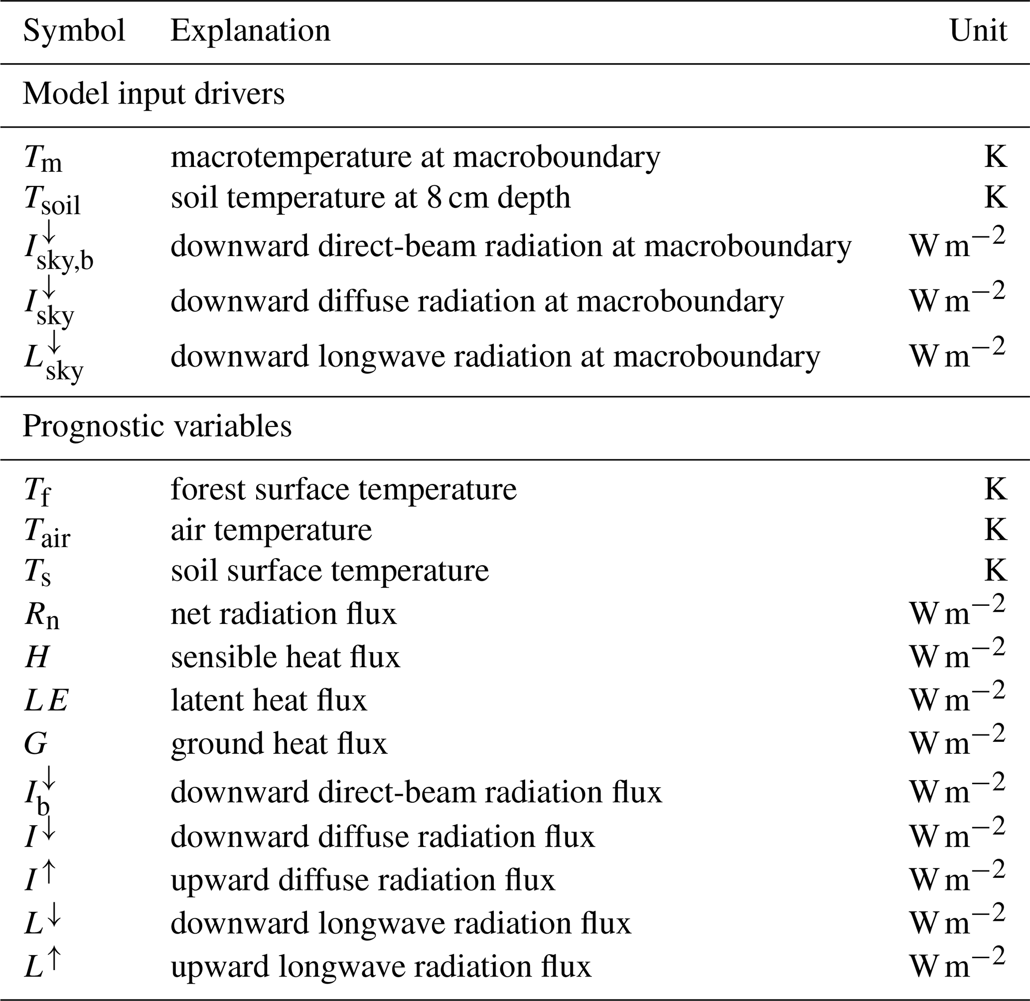
All meteorological variables, including microclimate air and soil temperature, shortwave and longwave radiation, and macroclimate air temperature, were aggregated to hourly means. Macroclimatic air temperature, soil temperature, and radiative fluxes served as model inputs, whereas microclimate air temperature data were used for calibration and validation. All model input drivers and voxel-specific outputs (prognostic variables) of temperatures and fluxes are summarised in Table 2.

Table 2 Model input drivers and prognostic variables in the ForEdgeClim framework. The table summarises all external variables required to run the model, including radiative and meteorological inputs, as well as all prognostic variables iteratively resolved during the simulation. Prognostic variables are modelled for each voxel.

4 Model evaluation

4.1 Sensitivity analysis

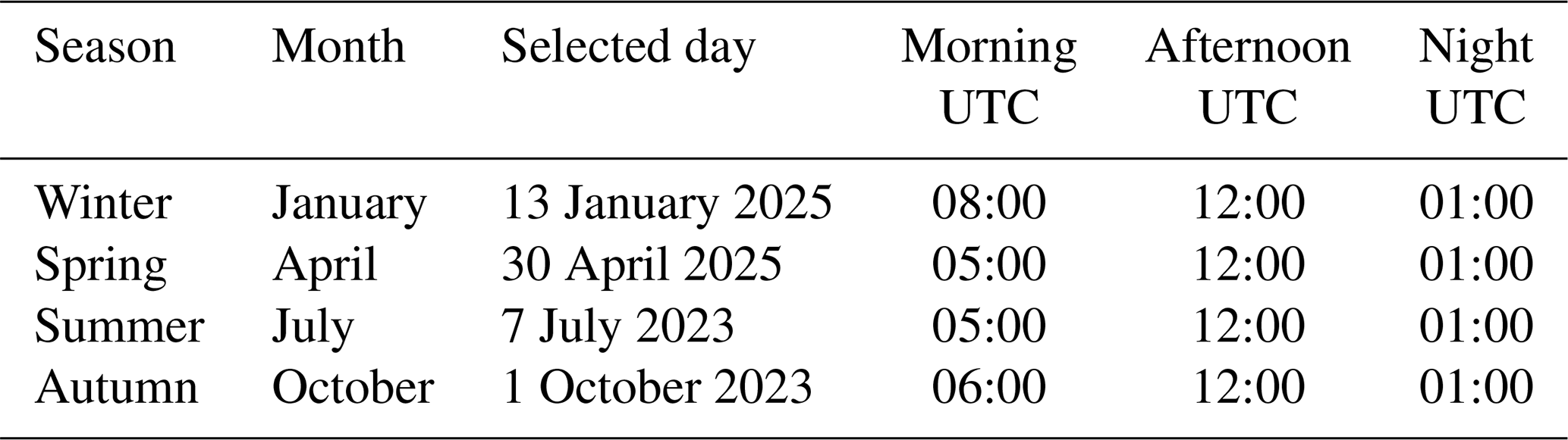
To investigate the most important drivers of the model outputs, we applied a Sobol sensitivity analysis (Sobol', 2001). This variance-based method quantifies both first-order effects and higher-order parameter interactions, making it well suited for ForEdgeClim, where radiative transfer, heat exchange, and structural parameters interact non-linearly across three spatial dimensions. The analysis was conducted for four representative months corresponding to the four seasons – January (winter), April (spring), July (summer), and October (autumn) – to capture seasonal variability in parameter sensitivity.

Because the forest buffering capacity is strongest under stable conditions with high direct solar radiation (Zellweger et al., 2019; De Frenne et al., 2021), which maximise edge-to-core contrasts and are the focus of this study, we selected, for each month during July 2023–April 2025, the day with the highest amount of direct sunlight and the smallest hourly variation in that light. This was done by identifying the day with the highest mean direct sunlight and the smallest mean hourly change in direct sunlight. We expect that a Sobol analysis conducted at time points with lower buffering capacity would yield slightly different results, but this study specifically targets conditions under which edge effects and buffering capacity are most pronounced.

For each of the four sunniest days, we performed the Sobol analysis at three distinct time points: morning, afternoon, and night. These time points were chosen according to the number of daylight hours in each season. In each season, the morning corresponds to approximately one hour after sunrise, the afternoon to the period shortly after solar noon (12:00 UTC), and the nighttime to 01:00 UTC, providing a consistent representation of night across all seasons.

Including the morning time point might be particularly insightful along the horizontal transect, as the forest edge is located on the eastern side where the sun rises. By focusing on this period, the Sobol analysis captures how parameter influence may change when lateral radiation enters the forest. Moreover, the morning marks the onset of warming, while solar noon approximately coincides with the maximum incoming radiation. Together, these time points enable a detailed examination of the temperature gradient along both the horizontal and vertical transect lines within the Sobol framework. The selected time points are summarised in Table 3.

Table 3 Time points (UTC) on which Sobol analyses were run for each season.

After performing the Sobol analysis for each season and time point, Sobol indices were computed for six key metrics along the horizontal and vertical transect lines. For each transect line, this resulted in a total of $\mathrm{4}\times \mathrm{3}\times \mathrm{6}=\mathrm{72}$ quantities of interest (QoIs): four seasons, three time points, and six metrics. The metrics considered were the mean temperature (≈T), the standard deviation of temperature (σT), and the edge-to-core temperature gradient (∇T), each computed for both air and forest surface temperatures. To synthesise the Sobol sensitivity results for both air temperature and forest surface temperature, parameter contributions were averaged across all combinations of metrics, time points, and seasons – here collectively referred to as conditions.

Sobol indices were calculated in both their normalised and non-normalised forms. The normalised indices represent the proportion of the total-order variance in a QoI that can be attributed to a given parameter directly and its interactions among parameters of any order. These values allow direct comparison of the relative importance of parameters. The non-normalised indices, by contrast, quantify the absolute contribution of a parameter to the total variance, expressed on the original scale of the variance itself. This distinction is important: while the normalised form highlights the ranking of parameter influence, the non-normalised form shows how much variance each parameter actually explains in absolute terms, enabling comparisons across different QoIs whose variances may differ substantially.

In this probabilistic analysis, each of the 25 model parameters was assigned a uniform distribution defined by its minimum and maximum values. The parameter ranges were taken from the literature and are summarised in Table 1. We generated 400 parameter sets using Latin hypercube sampling (LHS).

4.2 Calibration and validation

4.2.1 Calibration

To calibrate the model, we used the Covariance Matrix Adaptation Evolution Strategy (CMA-ES) (Hansen and Ostermeier, 2001; Hansen et al., 2003), a stochastic, derivative-free evolutionary optimisation algorithm well-suited for non-linear and non-convex objective functions. It can be used when the search space is complex, discontinuous, or contains multiple local optima (Auger and Hansen, 2005). These properties make it highly appropriate for calibrating process-based environmental models, where objective functions are often non-smooth and derivative information is unavailable or unreliable (Keating et al., 2010). Moreover, CMA-ES has demonstrated strong and robust performance in relatively low-dimensional parameter spaces (Hansen, 2006), which aligns with the scope of our calibration problem.

Following the Sobol sensitivity analysis (Sect. 4.1), only parameters that together explain more than 65 % of the total variance of any condition were optimised, whereas all others were fixed at their mean literature values (Table 1). Calibration was conducted separately for each season using three 24 h periods that captured distinct radiation regimes: the sunniest day, the cloudiest day, and the day with the strongest solar fluctuations over the period July 2023–April 2025 (Table 4 and, e.g., Fig. C2). Cloudy hours were defined as those with a difference of less than 5 W m⁻² between total and diffuse radiation. These three days were selected to represent the dominant microclimatic contexts each season experiences and to ensure strong constraints on model processes.

In addition, a year-round calibration was performed using all 12 selected days (three per season). This allowed evaluation of whether a single parameter set can describe microclimatic processes consistently across the full annual cycle, and how its performance compares to the seasonal calibrations.

The objective function was the root mean square error (RMSE) between the simulated and observed air temperature. Observations were obtained from 15 TOMST TMS-4 sensors at 15 cm height (ten positions along the central horizontal transect line and five vertical positions along the tower, purple dots in Fig. 1). Each seasonal calibration thus used 1080 observations ($\mathrm{3}\mathrm{d}\times \mathrm{24}\mathrm{h}\times \mathrm{15}\mathrm{sensors}$). To ensure a balanced influence of horizontal and vertical gradients, the five tower sensors were upweighted by a factor of two in the RMSE calculation.

To allow a consistent comparison of model performance across temporal scales, for all seasonal calibrations and the year-round calibration, the following performance metrics were computed against observations from TOMST TMS-4 temperature sensors: RMSE, mean error (ME), standard deviation of the residuals (SD), coefficient of determination (R²), and Nash–Sutcliffe Efficiency (NSE).

The TOMST TMS-4 sensors used for air temperature observations can occasionally be affected by sunflecks, where direct sunlight locally heats the sensor and biases the measurements due to overheating of the radiation shield. For all 24 h periods listed in Table 4, data was manually checked for sunflecks, by inspecting for abnormal temperature increases relative to neighbouring sensors. No sunflecks were detected on the most cloudy or the most solar fluctuating days; however, two affected measurements (10:00 UTC and 11:00 UTC) were identified on the sunniest summer day (7 July 2023) for one ground sensor located in an open canopy area. These data points were excluded from the calibration.

Table 4 Three specific days on which CMA-ES calibrations were run for each season.

CMA-ES was run until convergence, with a maximum of 50 generations (7 offspring per generation). The number of generations required for convergence varied among seasons, reflecting seasonal differences in parameter sensitivity and model behaviour.

Although model calibration is commonly performed on a larger dataset than model validation, we adopted the opposite strategy. The three seasonally selected calibration days represent distinct and highly informative radiation regimes – sunny, cloudy, and strongly solar fluctuating – which provide stronger constraints on the underlying processes than a larger number of less diagnostic days. Using a small but diverse calibration set also reduces the risk of overfitting to the conditions of a particular month or synoptic situation. Validation was instead carried out on full representative months for each season (Sect. 4.2.2), allowing a much more stringent assessment of parameter robustness under the full range of seasonal meteorological variability. This design ensures that parameters are calibrated on physically meaningful situations while being evaluated on all conditions relevant for model application.

4.2.2 Validation

Model validation was performed separately for each season using all days of a representative month: July 2023 (summer), October 2023 (autumn), January 2025 (winter), and April 2025 (spring). These months capture a wide range of microclimatic conditions and include the sunniest calibration day for each season. The seasonal validation sets contained 10 800 (or 11 160) observations ($\mathrm{30}/\mathrm{31}\mathrm{d}\times \mathrm{24}\mathrm{h}\times \mathrm{15}\mathrm{sensors}$).

A year-round validation was also conducted using the combined dataset of all four representative months. This enabled assessment of how well the parameter set from the year-round calibration generalises across the full annual cycle.

Validations were run using both calibrated and uncalibrated parameter sets. In calibrated runs, only the most influential parameters identified through the Sobol analysis were replaced by their optimised values; all other parameters were kept at their mean literature values. Uncalibrated runs used mean literature values for all parameters.

For all validations – seasonal and year-round – the same performance metrics were computed by comparing modelled air temperatures with measurements from TOMST TMS-4 sensors (RMSE, ME, SD, R², and NSE), enabling direct comparison of model accuracy and robustness under different calibration strategies.

Comparison of calibrated and uncalibrated runs allowed assessment of the representativeness of literature-derived parameter ranges. Parameter estimates falling near the boundaries of their prior distributions indicate that published ranges may be insufficiently constrained, whereas calibrated values lying well within these bounds suggest that literature-based parameters provide a reliable basis for model application.

To assess the potential influence of wind-driven processes not explicitly represented in the model, model residuals were analysed as a function of observed wind speed and distance to the forest edge.

In addition, to evaluate the uncertainty associated with forest surface temperature predictions, the Sobol parameter ensemble was propagated through the model, and the resulting distributions of simulated surface temperature were analysed across all validation conditions.

5 Results

5.1 Prognostic variables

As a proof of concept, we present several results from runs of ForEdgeClim on 8 July 2023, the hottest day of that year. These results were produced using the initial, uncalibrated, yet literature-based, parameter set. They are presented here solely to demonstrate the prognostic patterns and internal dynamics simulated by ForEdgeClim; the calibration of model parameters and subsequent validation analysis follow in Sect. 5.3.

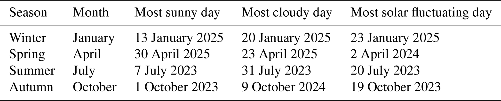
At 14:00 UTC, strong spatial variability in total downward shortwave radiation – comprising both the direct-beam component and the diffuse downward flux – becomes apparent, with deeper light penetration in the western forest core where ash-dieback-induced canopy gaps increase transmission (Fig. 2a). In contrast, radiation is rapidly attenuated in denser canopy regions, while reduced canopy density along the eastern forest edge allows additional light to enter. The total shortwave radiation reaching the forest floor shows a similarly heterogeneous spatial structure. The highest ground-level fluxes occur at the eastern side of the transect, where the open street adjacent to the forest receives substantially more light than the forest itself. Within the forest, increased radiation levels are primarily associated with canopy gaps located further toward the core rather than directly at the edge, indicating that these interior structural openings provide additional pathways for light to penetrate to the ground.

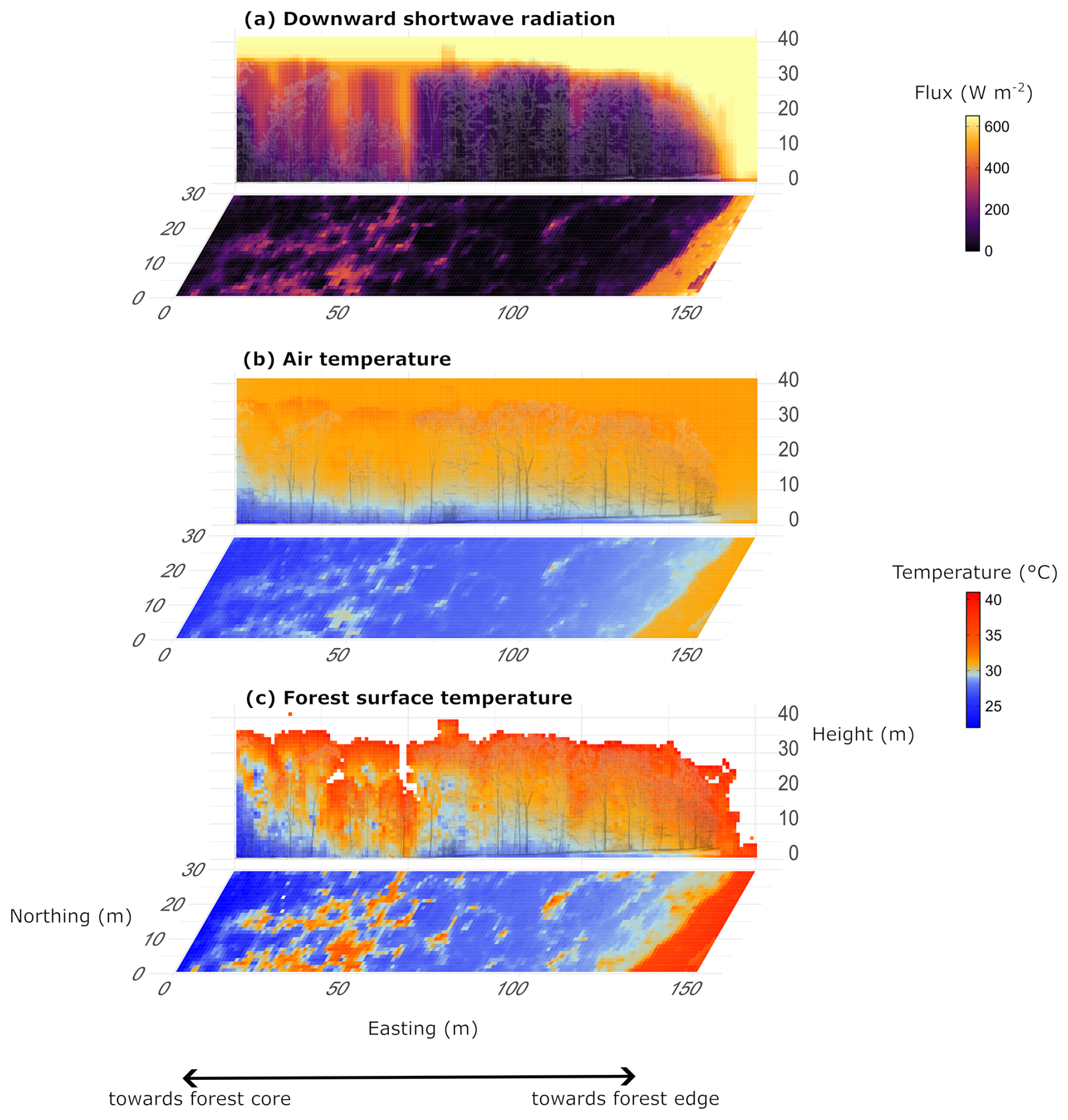
Figure 2 Modelled prognostic variables on 8 July 2023 at 14:00 UTC. (a) Downward shortwave radiation, (b) air temperature, and (c) forest surface temperature. Air temperature represents the temperature of the air volume within each grid cell, governed by radiative forcing and sensible and latent heat exchange with neighbouring air cells and forest surfaces. Forest surface temperature represents an effective density-weighted temperature of leaf and woody element surfaces, which directly absorb radiation and exchange energy with the surrounding air through sensible and latent heat fluxes. In this 3D representation, all vertically oriented planes (in the 2D vertical plane of this figure) represent averages of all slices along the north–south axis. The horizontal plane in each subplot shows the model output at ground level, representing the layer from 0–1 m above the soil surface. In the vertical planes, the background displays a slice along the central TLS transect line, illustrating the forest structure point cloud.

Clear spatial patterns also emerge in the simulated air temperature field, with macroclimate conditions outside the forest transect reaching around 31 °C (Fig. 2b). Local warming occurs near the canopy top due to leaf absorption and re-emission of radiation, whereas the shaded understorey exhibits pronounced cooling. A horizontal temperature gradient is present in the lower forest layers, with air temperatures decreasing from the edge toward the core.

Forest surface temperatures show similar large-scale patterns but reach substantially higher values, up to approximately 40 °C (Fig. 2c). Warmer conditions in the upper canopy contrast with much cooler surfaces in shaded and near-ground areas. As with the air temperature field, a horizontal gradient is visible, with declining temperatures from the forest edge toward the core, although spatial differences are more pronounced due to heterogeneity in absorbed radiation.

Air temperature dynamics differ clearly between the forest core, the forest edge, and the open area outside the forest (Fig. 3). Temperatures at the edge consistently rise faster during the day than those in the core, and their diurnal amplitude is markedly larger. This contrast is particularly well captured by the model during the morning hours, when edge–core temperature gradients are strongest. During this period, modelled gradients closely match observations, indicating that the model successfully resolves the edge-to-core temperature signal.

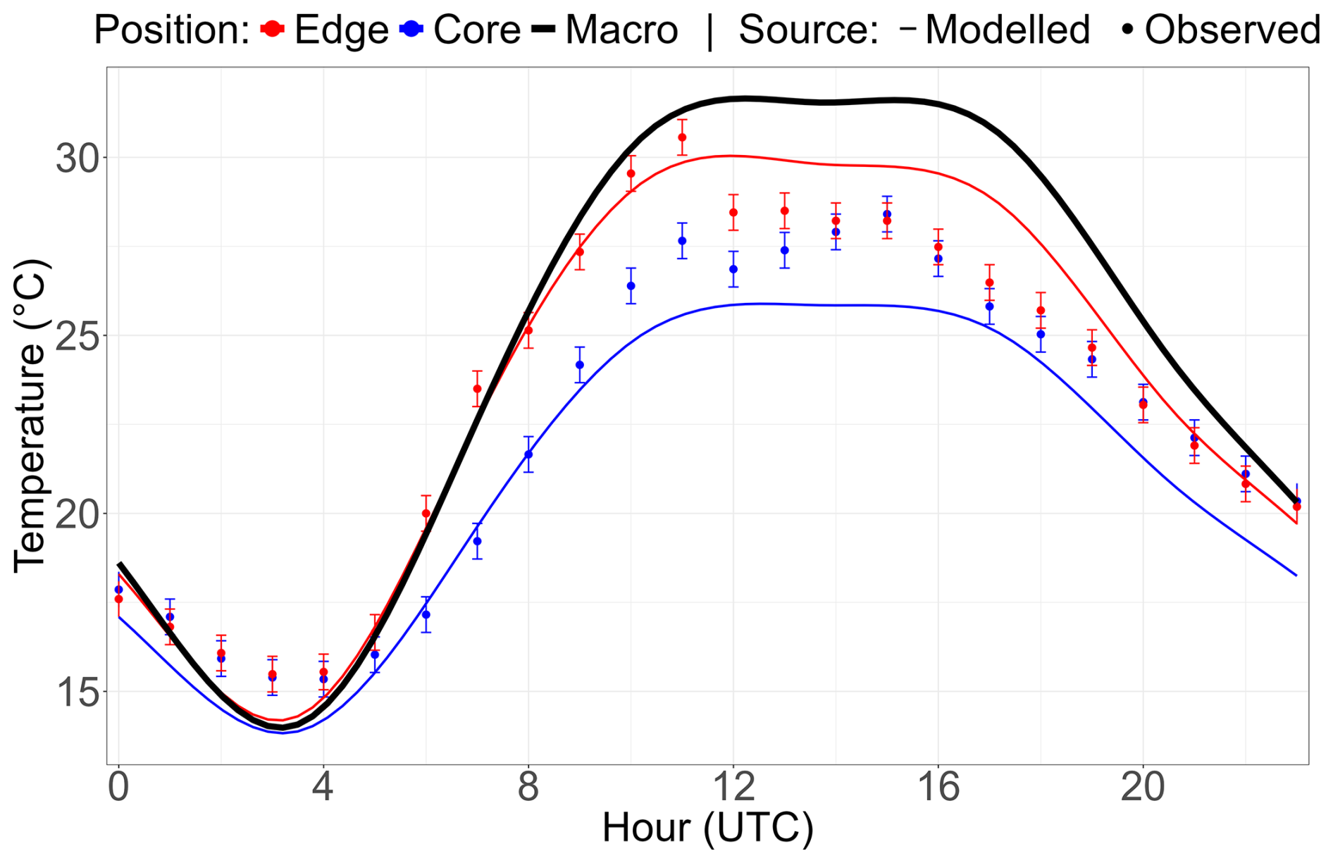
Figure 3 Time series of modelled (lines) and observed (points) air temperature for the forest core (blue) and forest edge (red) on 8 July 2023 (24 hourly time points), together with the observed macrotemperature used as model driver (thick solid black line). Model values represent voxels immediately above the ground surface (voxel volume = 1 m³), while TOMST observations were recorded at 15 cm height. Modelled temperature curves are interpolated using a cyclic cubic spline. Error bars on the TOMST observations indicate the logger accuracy (±0.5 °C).

Observed temperatures at the forest edge and core converge in the afternoon, whereas the model maintains a stronger edge–core contrast. This indicates that, for this particular day, the model overestimates spatial temperature gradients when the observed system becomes more thermally homogeneous.

This pattern reflects stronger exposure to radiative and advective forcing at the forest edge, whereas conditions within the forest interior remain more buffered throughout the day.

In Fig. 3, observed temperatures at the forest edge show a more abrupt decline after solar noon than simulated temperatures, potentially reflecting the sudden loss of direct lateral sunlight when the sun angle shifts and the sensor becomes shaded by the canopy. This sharp transition is captured by the in situ measurements but is smoothed in the model, which represents radiative forcing and heat exchange at the voxel scale rather than resolving sensor-scale shading effects. The convergence of observed temperatures in the afternoon during this period may further reflect increased turbulent mixing within the forest, which is not explicitly accounted for in the model and may contribute to the persistence of stronger gradients in the simulations.

A comprehensive evaluation of modelled versus observed edge–core temperature gradients across all simulated time steps is presented in Sect. 5.3.2, combining an assessment of the agreement in gradient magnitude with an analysis of the model's ability to resolve spatial temperature contrasts relative to its uncertainty.

5.2 Sensitivity analysis

The resulting patterns from the Sobol sensitivity analysis reveal clear differences in parameter influence for air temperature and forest surface temperature along the horizontal transect (Fig. 4).

Figure 4 Sobol sensitivity analysis of parameter contributions to (a) air temperature variance and (b) forest surface temperature variance along the horizontal transect. Air temperature represents the temperature of the air volume within each grid cell, forest surface temperature represents an effective density-weighted temperature of leaf and woody element surfaces. The parameters i_m, i_s and i_f, representing the distances of influence from the macroenvironment, soil surface, and forest surface, respectively, are shown in blue. The parameters g_m, g_s and g_f, representing convection from the macroenvironment, soil surface, and forest surface, respectively, are shown in orange. The parameters k_s (soil conductance), h (air heat conduction coefficient) and p (fraction of net radiation R_n absorbed by the soil surface) are shown in red. SW refers to all shortwave RTM parameters (nine parameters), and LW to all longwave RTM parameters (seven parameters). ≈T denotes the mean temperature, σT the temperature standard deviation, and ∇T the temperature gradient from forest core to edge. For further details on the model parameters, see Table 1.

The sensitivity patterns for air temperature reveal a strong dependence on three heat-transfer parameters: i_m, i_s, and k_s, representing the distance of influence from the macroenvironment, the distance of influence from the soil surface, and the soil conductance, respectively (Fig. 4a). Across all conditions, these parameters together account for 67 %–76 % of the total output variance along the horizontal transect. On average, their combined contribution amounts to 70.8 % (95 % CI: 68.4 %–73.2 %), indicating that model sensitivity is consistently concentrated within a small subset of parameters.

Shortwave and longwave radiation parameters explain a smaller share of the model output variance overall (2.7 %–5.8 %), but their influence varies systematically with environmental context (Fig. 4a). Longwave processes dominate during the night and morning, in both cases accounting for 2.8 % of the variance, whereas shortwave processes are most influential during the day, explaining 3.5 % of the variance. Seasonally, longwave effects reach their maximum in summer (3.4 %) and shortwave in spring (2.6 %). Among all evaluated metrics, radiative processes have the greatest impact on the temperature gradient (5.8 %), because incoming radiation from the forest edge drives the horizontal thermal gradient.

A distinct sensitivity pattern emerges for forest surface temperature (Fig. 4b). The parameter g_f, which represents forest convection, contributes far more strongly than in the air temperature case and explains the largest share of the total variance (8.7 %–32 %). The parameters i_m and i_s also remain influential (23 %–46 %), but radiative transfer parameters gain importance relative to the other heat-transfer processes (11 %–30 %), indicating that radiation exerts a more direct control on forest surface temperature. Despite these shifts, the heat-transfer parameters i_m, i_s, and g_f still dominate the overall sensitivity, together accounting for 44 %–64 % of the total model output variance.

When performing the same analysis for both air temperature and forest surface temperature along the vertical line, we observed consistent patterns (Fig. C3). For air temperature (Fig. C3a), the parameters i_m, i_s, and k_s dominate model sensitivity, together explaining 67 %–72 % of the total model output variance. On average, their combined contribution amounts to 70.3 % (95 % CI: 68.0 %–72.5 %), again, indicating that model sensitivity is consistently concentrated within a small subset of parameters. For forest surface temperature (Fig. C3b), the results along the vertical line differ slightly from those along the horizontal line. The parameters i_m and g_f remain the most influential (28 %–56 %), but i_s loses its position as third most influential parameter. Instead, both the longwave and shortwave parameters gain importance, together explaining 22 %–33 % of the total output variance.

For both the air and forest surface temperature, radiative transfer parameters are more influential along the vertical transect (2.4 %–9.3 % and 22 %–33 %, respectively) than along the horizontal transect (2.7 %–5.8 % and 11 %–30 %). This stronger influence along the vertical transect reflects the direct control of radiative parameters over the local canopy and forest surface energy balance driven by vertically incident radiation. Along the horizontal transect, the relative contribution of radiative parameters to output variance is reduced due to stronger modulation by lateral heat exchange processes.

Based on the sensitivity patterns, the three dominant heat-transfer parameters, i_m, i_s, and k_s, were selected for model calibration. The remaining 22 parameters were fixed at their mean values from the uniform distributions reported in literature (Table 1). The parameter g_f was not included in the calibration procedure because the calibration is based on observed air temperature, which is largely insensitive to variations in g_f (Figs. 4a and C3a). Including this parameter would therefore not meaningfully constrain the model. If calibration were instead performed against forest surface temperature, g_f would become an essential parameter to tune, as it exerts the strongest influence on the variance of that variable.

The non-normalised Sobol indices (not shown) showed similar parameter ranking across the QoIs, indicating that normalisation does not affect inferred parameter importance. However, three QoIs related to vertical forest surface temperature gradients showed substantially higher absolute sensitivities than the other QoIs (approximately 4–10 times higher). As forest surface temperature is not used for calibration, this does not affect parameter selection.

To assess the robustness of the Sobol sensitivity indices, a convergence analysis was performed by comparing results obtained with 200 and 400 Latin hypercube samples (Fig. C4). The total-order Sobol indices of the dominant parameters for both air temperature (i_m, i_s, and k_s) and forest surface temperature (i_m, i_s, and g_f), as well as their combined contribution, showed only minor differences between the two sample sizes when averaged across all conditions (i.e., seasons, times of day, and metrics) along both horizontal and vertical transects. This indicates that the sensitivity estimates are stable and sufficiently converged for the purpose of identifying the main drivers of model variability.

5.3 Calibration and validation

5.3.1 Calibration

The calibrated parameter values and associated performance metrics for each season and for the full year are summarised in the upper part of Table 5, including the root mean square error (RMSE, the objective function), mean error (ME), standard deviation of the residuals (SD), coefficient of determination (R²), and Nash–Sutcliffe efficiency (NSE).

Across seasons and throughout the year, several parameters converged towards the upper bounds of their uniform prior distributions during calibration. In the winter, spring, and annual calibration, the parameter k_s approached its maximum allowed value of 2.2 $\mathrm{W}{\mathrm{m}}^{-\mathrm{1}}{\mathrm{K}}^{-\mathrm{1}}$. In the winter, summer, and annual calibration, the parameter i_m similarly converged towards its upper bound of 60 m. These patterns indicate that the optimum lies at, or beyond, the upper bounds of the prescribed prior ranges for k_s and i_m and may not adequately capture the effective values required to reproduce the observed microclimate dynamics at the study site. By contrast, the parameter i_s remained close to the centre of its literature-derived parameter range, across the annual and all seasonal calibrations.

The annual residual-based performance metrics (RMSE, ME, and SD) converged to values comparable to the seasonal metrics' mean (resp. 1.24, 0.06, and 1.24 °C), reflecting the integration of contrasting seasonal dynamics. In contrast, both efficiency-based metrics (R² and NSE) attained their highest values for the annually calibrated parameter set (resp. 0.97 and 0.97). This indicates that, while annual calibration does not minimise absolute errors for individual seasons, it exposes the model to a wider range of thermal conditions and spatial gradients. This leads to parameter values that better capture the structure and variability of the temperature field, as reflected by higher R² and NSE values.

Table 5 Model parameter values and statistical performance across calibration and validation datasets. See Table 1 for a more detailed definition of the parameters. Uncalibrated, literature-based parameter ranges are indicated between square brackets in the parameter labels.

Over all seasons and throughout the year, the convergence behaviour of the CMA-ES optimisation process reveals a clear reduction in the objective function (RMSE) during the early generations, followed by stabilisation as the algorithm approaches its optimum (e.g., Fig. C5a). This pattern indicates that no further improvement in model fit is achieved once the RMSE curve has levelled off.

An additional view of convergence is obtained by examining the distribution of sampled parameter sets in a principal component space. A principal component analysis (PCA) performed across all generations and offspring shows that the spread of parameter sets narrows progressively, with points clustering more tightly as optimisation proceeds (e.g., Fig. C5b). This contraction of the parameter cloud reflects a strong concentration of sampling around the converged region of the parameter space.

5.3.2 Validation

To provide context for the aggregated validation statistics, we first examine model behaviour for a representative warm summer day (8 July 2023) in the Aelmoeseneiebos forest by comparing simulated horizontal and vertical air temperature gradients from annually and seasonally calibrated ForEdgeClim runs with TOMST TMS-4 observations (Fig. 5). Model outputs (solid and dashed lines) are evaluated against sensor measurements (dots). Both calibration strategies capture the main observed temperature patterns and spatial gradients. For this summer day, the annually calibrated simulation shows closer agreement with the observed gradients, whereas the seasonally calibrated model likely overfits season-specific noise. This suggests that annual calibration captures more robust, process-level behaviour.

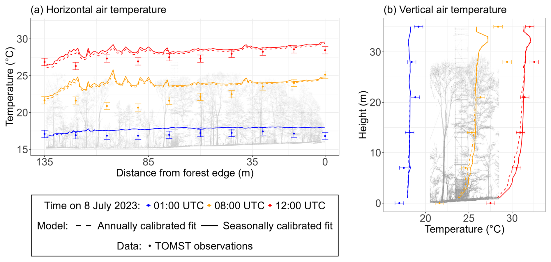
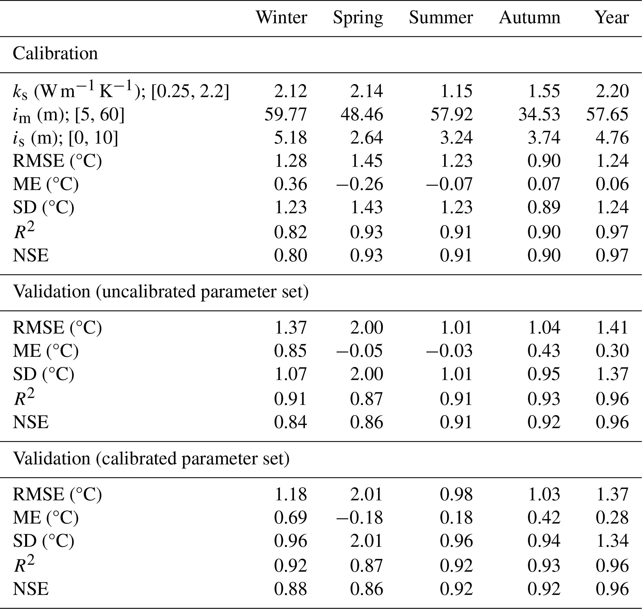
Figure 5 (a) Modelled (annually calibrated and seasonally calibrated) and observed air temperature from the forest edge to the forest core. Model values represent voxels immediately above the ground surface (voxel volume = 1 m³), while TOMST observations were recorded every 15 m at 15 cm height. (b) Modelled and observed air temperature along the central vertical line at the tower position. Model values include all voxels intersecting this vertical tower line (voxel volume = 1 m³), and TOMST observations were recorded every 7 m.
Error bars on the TOMST observations indicate the logger accuracy (±0.5 °C). All values correspond to 8 July 2023 (UTC). The background shows a slice of the central TLS transect line, illustrating the forest structure point cloud.

At noon (12:00 UTC), a decrease in air temperature from the forest edge towards the core was observed, driven by canopy shading that limits radiative heating of the lower forest strata (Fig. 5a). The forest structure further buffers heat transfer by restricting the penetration of warm macroclimatic air entering near the forest edge into the interior. While most of the absolute temperatures are overestimated, the model reproduces the magnitude and direction of the observed edge-to-core gradient.

During the night (01:00 UTC), spatial temperature differences diminished considerably, with a relatively uniform and cool temperature field extending from edge to core (Fig. 5a). This reflects the reduced thermal contrast under low-radiation conditions. The small positive bias during this period suggests that nocturnal cooling processes may be underestimated in the current model configuration.

In the morning (08:00 UTC), a horizontal gradient reappeared as lateral radiation entered the forest from the east, resulting in increased warming near the edge (Fig. 5a). This highlights the role of lateral radiation in shaping edge microclimates. The temperature contrast between the forest interior and the external environment was strongest during this period, after which heating became more spatially uniform later in the day. The relatively large discrepancy between modelled air temperatures and TOMST observations during the morning period, particularly in the vicinity of forest gaps (distance from the forest edge of approximately 110 m), is likely amplified by differences in effective measurement height. Model outputs represent mean air temperature within 1 m³ voxels, whereas TOMST observations are recorded at 15 cm above the ground. During the morning transition, radiative forcing and heat transfer may already have warmed the upper part of the lowest 1 m forest layer, while temperatures closer to the ground remain cooler, resulting in larger apparent differences between modelled and observed values.

Vertical air temperature profiles reveal distinct stratification patterns across the three selected time points (Fig. 5b). During the night (01:00 UTC), temperatures remain nearly uniform throughout the vertical column, reflecting stable conditions in the absence of radiative forcing. As the sun rises (08:00 UTC), a vertical gradient develops, with warming concentrated in the upper canopy. This vertical stratification persists through midday (12:00 UTC), indicating sustained thermal differentiation within the canopy during daytime conditions.

For the winter season, the differences in statistical metrics are most pronounced when comparing the calibrated validation set with the uncalibrated validation set. A modest improvement is observed when the calibrated parameter set is applied, as evidenced by higher values of both the coefficient of determination (R²) and the Nash–Sutcliffe efficiency (NSE). Consistent with this, the residuals exhibit smaller deviations for the calibrated simulations, with notably reduced root mean square error (RMSE), mean error (ME), and standard deviation of the residuals (SD) indicating an overall increase in model accuracy (Fig. 6). An analysis of the residuals grouped by hour of the day shows that the smallest discrepancies between observed and modelled temperatures occur during daytime hours (Fig. 6b). In addition, calibration leads to a marked improvement in model performance at locations closer to the forest core, where canopy gaps are more common (Fig. 6c), as well as at positions near the forest floor and just above the canopy (Fig. 6d). Overall, these results indicate that the calibration improves model performance in a process-specific manner, particularly for radiation–structure interactions, rather than through a uniform error reduction across space and time.

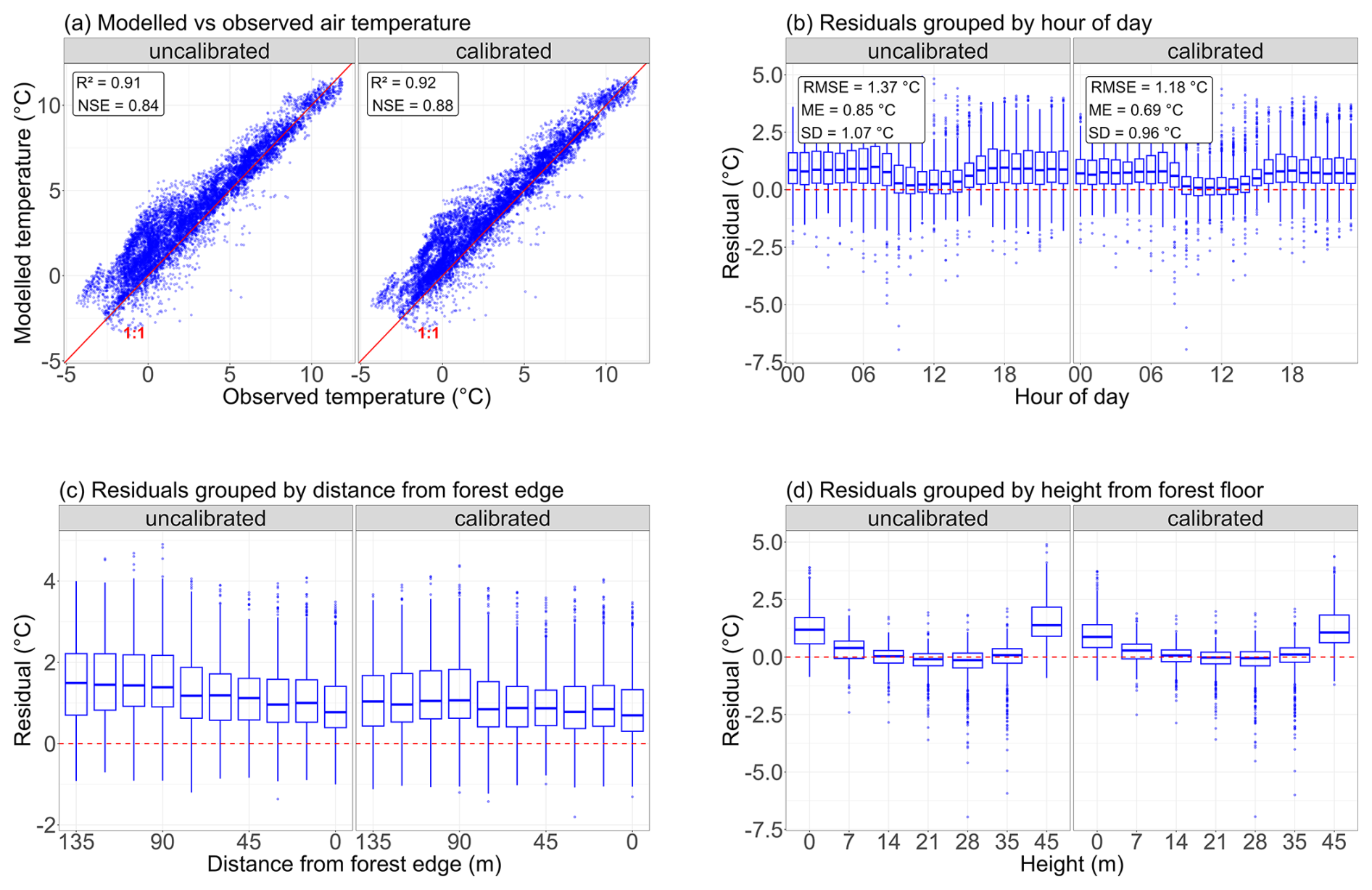
Figure 6 Model validation for the winter season. (a) Comparison between modelled and observed air temperature for simulations using calibrated and uncalibrated parameter sets. Panels (b–d) show the corresponding model-observation residuals for both parameterisations, grouped by hour of the day (b), distance from the forest edge (c), and height above the forest floor (d).

In spring, summer, autumn, and for the annual period, the distinction between calibrated and uncalibrated performance is less pronounced, indicating that the application of the calibrated parameter set leads to only marginal changes in model performance. A full overview of validation statistics for all seasons and throughout the year is provided in Table 5.

The validation statistics show that residual-based performance measures for the annual validation sets (both calibrated and uncalibrated) converge towards the mean of the seasonal residuals. In contrast, both R² and NSE consistently attain their highest values for the annual period, indicating a more consistent representation of observed temperature variability across independent conditions. While seasonally calibrated parameter sets can improve agreement with observations under specific conditions, their performance across independent validation periods is more variable. This suggests that seasonal calibration optimises model behaviour for targeted conditions, whereas annual calibration yields a more generalisable parameterisation across contrasting meteorological regimes.

Overall, both the calibrated and uncalibrated configurations reproduce observed air temperature patterns with modest errors across seasons and throughout the year. RMSE, ME, and SD values remain low, while R² and NSE indicate that a substantial fraction of the observed variability is captured. For comparison, RMSE values reported during the validation of microclimf range between 0.69 and 2.9 °C (Maclean, 2025), whereas in this study RMSE values across both configurations range between 0.98 and 2.01 °C.

Across the full simulation period, modelled and observed edge–core temperature gradients show a moderate level of agreement, with modelled gradients broadly following the observed direction (Fig. 7a). However, substantial scatter and clear seasonal differences indicate that the model has limited ability to accurately reproduce the magnitude of these gradients across all conditions, even though the presence of spatial gradients is generally captured.

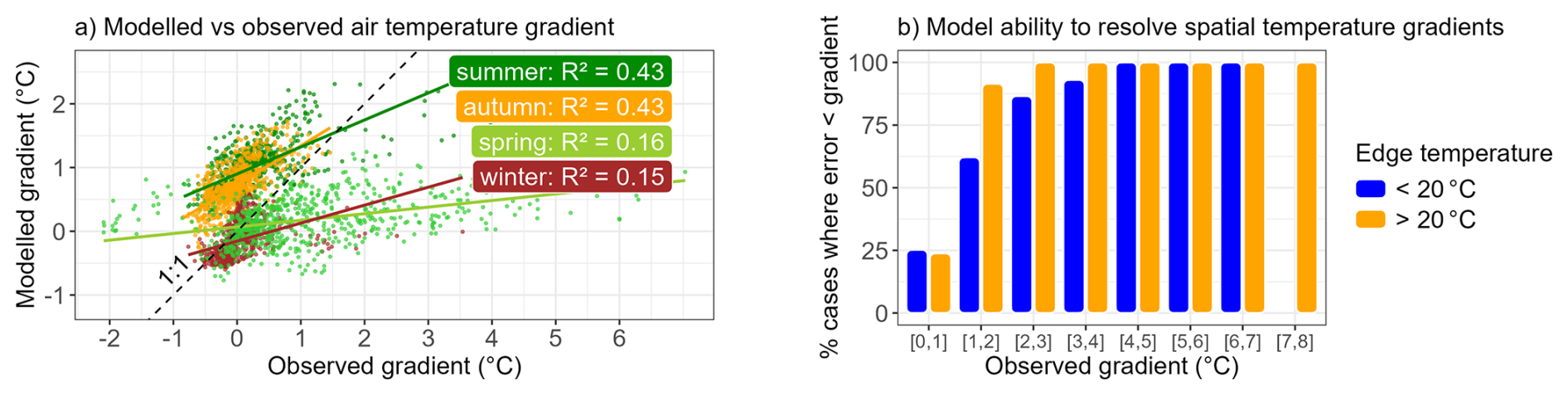
Figure 7 Comparison of modelled and observed edge–core air temperature gradients across all simulated time steps using a single annually calibrated parameter set. (a) Relationship between modelled and observed gradients, coloured by month (brown: winter, light green: spring, dark green: summer, orange: autumn). The dashed line indicates the 1:1 relationship. (b) Model performance as a function of observed gradient magnitude, expressed as the percentage of cases in which the absolute mean error (AME) between modelled and observed gradients is smaller than the observed gradient. Bars are aggregated across bins of observed gradient values, with blue and orange indicating cooler (≤20 °C) and warmer (>20 °C) edge temperatures, respectively.

This variability in model performance can be explained by differences in the magnitude of the observed gradients. The proportion of cases in which model error is smaller than the observed gradient increases markedly with gradient magnitude (Fig. 7b). For larger gradients, the majority of cases fall below the threshold where model error exceeds the observed gradient, indicating that the model is generally able to resolve pronounced spatial temperature differences. In contrast, for small gradients (e.g., below approximately 1 °C), the proportion of cases where model error exceeds the signal is substantially higher, indicating limited ability to resolve weak spatial contrasts.

This pattern reflects the fact that edge–core temperature differences approach zero under near-isothermal conditions, where even small absolute model errors can exceed the signal. As a result, the model's ability to resolve weak spatial gradients is inherently limited under these conditions due to a low signal-to-noise ratio, rather than a systematic misrepresentation of spatial patterns.

Overall, these results indicate that the model is capable of resolving spatial temperature gradients when they are sufficiently pronounced, but that caution is required when interpreting simulated gradients under conditions where observed differences are small. This behaviour is consistent with the calibration strategy, which targets point-wise air temperature (RMSE) rather than explicitly constraining the edge–core temperature gradient.

5.3.3 Influence of wind speed on model residuals

In the current implementation of ForEdgeClim, wind-driven processes are not explicitly represented. To assess the potential influence of this omission, model residuals were analysed as a function of observed wind speed and distance to the forest edge (Fig. 8).

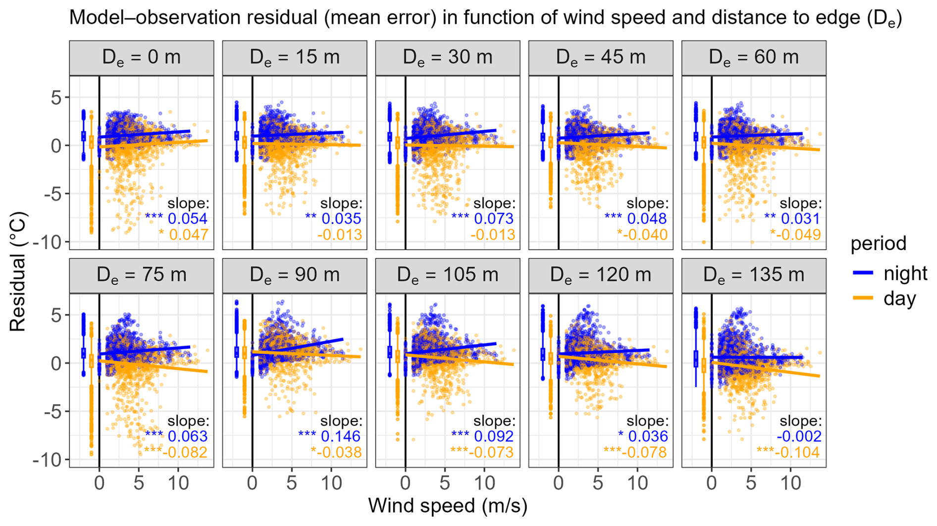
Figure 8 Relationship between model–observation residuals (mean error) and wind speed across distances from the forest edge to the forest core. Daytime hours are defined as 05:00–17:00 UTC and nighttime hours as 17:00–05:00 UTC. The dataset comprises the four seasons, represented by one month per season. Boxplots on the left side of each panel summarise the distribution of the data. Slopes of the linear relationships are indicated, with significance levels denoted as * p<0.05, ** p<0.01, and *** p<0.001, and no symbol indicating non-significant relationships.

Overall, the influence of wind speed on model residuals, both during night- and daytime, appears limited, as indicated by the relatively small slopes across all spatial positions ($\mathrm{1}\times {\mathrm{10}}^{-\mathrm{3}}-\mathrm{1}\times {\mathrm{10}}^{-\mathrm{1}}\mathrm{°}\mathrm{C}{\mathrm{m}}^{-\mathrm{1}}\mathrm{s}$ in absolute order of magnitude). This suggests that wind-driven processes are not a dominant control on model performance under the conditions considered here. However, across all distances, residuals consistently increase with wind speed during both daytime and nighttime, indicating that wind-related processes are not yet fully captured by the current model formulation. The analysis spans four seasons, each represented by one month, suggesting that these patterns are robust across a range of environmental conditions.

Model performance nevertheless shows a clear but non-monotonic spatial pattern. Residuals are relatively small near the forest edge, where exchange with the external macroenvironment (represented by g_m and i_m) directly constrains local conditions. This indicates that the parameterised macroenvironmental forcing is sufficient to capture first-order edge effects.

Further into the forest, discrepancies increase, with the largest slope occurring during nighttime at approximately 90 m from the edge, corresponding to a canopy gap. At this location, residuals clearly increase with wind speed. In the forest core, higher residuals are also observed at higher wind speeds, particularly during the day. This suggests that, while wind penetration is reduced, the simplified parameterisation of heat exchange between air, macroenvironment (g_m, i_m), soil (g_s, i_s), and forest structure (g_f, i_f) does not fully capture the complex and heterogeneous flow regimes that characterise dense forest interiors.

Across all locations, the largest residuals predominantly occur during daytime conditions and at intermediate wind speeds. However, these high residuals are mainly associated with a limited number of extreme values. In contrast, the majority of daytime observations form a dense cluster with relatively small residuals, generally lower than those observed during nighttime periods, consistent with Fig. 6b.

Overall, these results indicate that the use of fixed convection parameters and distances of influence is sufficient to represent first-order macroenvironmental exchange and edge-to-core temperature gradients under the temperate forest conditions considered in this study, but insufficient to capture the full spatial variability in wind-driven turbulence and mixing associated with canopy gaps and structurally complex forest interiors. At the same time, the relatively weak sensitivity of residuals to wind speed suggests that explicitly resolving wind processes would likely lead to only incremental improvements under the tested conditions. However, the transferability of the current parameterisation to more open, windy, drought-stressed, or structurally contrasting forest systems remains uncertain and would require additional validation.

5.3.4 Uncertainty in forest surface temperature predictions

To assess the implications of parameter uncertainty for forest surface temperature, the Sobol parameter ensemble was propagated through the model, and the resulting distributions of simulated surface temperature were analysed across all conditions along both the horizontal and vertical transect lines (resp. Figs. 9 and C6).

The resulting distributions are approximately bell-shaped, indicating a smooth and stable model response to parameter variation, without evidence of abrupt thresholds or regime shifts. However, the width of these distributions varies substantially between conditions, demonstrating that forest surface temperature remains weakly constrained in several cases, with the central 95 % range spanning approximately 0.02–11.29 °C for the horizontal transect line and 0.02–4.05 °C for vertical transect line.

This behaviour is consistent with the Sobol sensitivity analysis, which identified the forest heat transfer parameter g_f as a dominant contributor to surface temperature variance (8.7 %–32 %). As g_f does not influence air temperature and is therefore not constrained during calibration, its variability directly translates into uncertainty in surface temperature predictions.

The resulting uncertainty envelopes thus provide a quantitative measure of this lack of constraint and highlight the need for additional observational constraints to better resolve surface energy exchange processes.

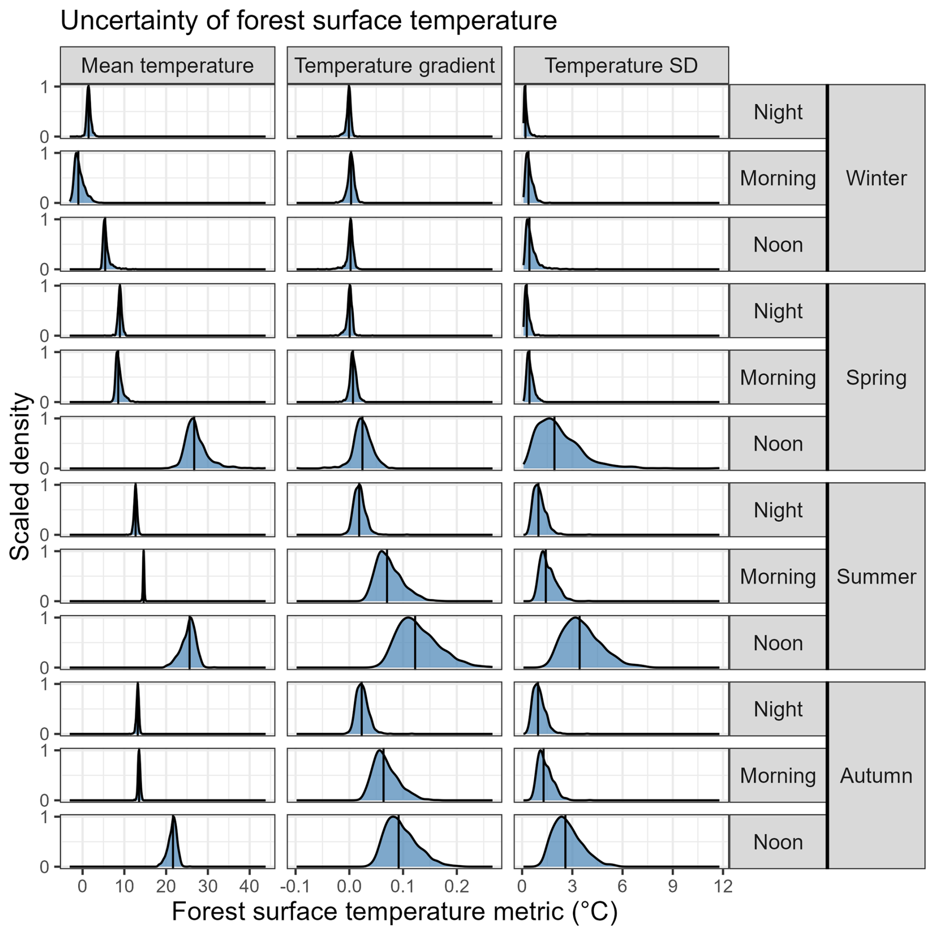
Figure 9 Uncertainty in forest surface temperature along the horizontal transect derived from the Sobol parameter ensemble. Density curves are scaled (peaks are set to a value of 1) to facilitate comparison of distribution shapes. Vertical lines indicate median values.

6 Discussion

We here present ForEdgeClim, a 3D, process-based microclimate modelling framework designed to explicitly resolve both vertical and lateral energy exchanges in fragmented forest landscapes where edge effects can be pronounced. The results demonstrate that explicitly accounting for boundary-driven heat transfer enables realistic simulation of edge-to-core temperature gradients at metre-scale resolution. At the same time, the analyses highlight that simplified representations of certain processes, particularly heat exchange and seasonal dynamics, remain key sources of uncertainty and opportunities for further model development.

6.1 Dominant processes shaping simulated microclimates

The sensitivity analysis indicates that heat-transfer processes exert the strongest influence on both simulated air temperature and forest surface temperature within the forest transect. Parameters controlling the spatial influence of the macroenvironment and the soil surface, together with the soil conductance and forest–air convection, explained the majority of variance in modelled temperatures. These findings suggest that interactions with the external atmosphere and the soil surface constitute the dominant controls on local air and surface temperature patterns, particularly under conditions of strong thermal contrast between the forest and its surroundings. This interpretation is further supported by an additional analysis of model residuals, which shows that discrepancies between modelled and observed temperatures increase with wind speed, particularly in open-canopy conditions such as forest gaps. This suggests that wind-driven turbulence and advective heat transport, which enhance atmospheric coupling, are not fully captured by the current parameterisation of heat exchange processes. At higher wind speeds, residuals also remain elevated in the forest interior, indicating that the simplified and spatially invariant parameterisation does not fully represent the complex flow regimes in dense canopy conditions.

More generally, these results indicate that in a 3D forest representation, microclimate variability is governed less by absolute radiative forcing than by the efficiency with which heat is exchanged across system boundaries. In ForEdgeClim, the forest edge and the soil–atmosphere interface act as dominant control surfaces that regulate both the magnitude and the spatial propagation of thermal signals into the forest interior. This underscores the importance of explicitly resolving boundary-driven fluxes in microclimate models, particularly when simulating edge-affected landscapes.

These findings are consistent with a substantial body of empirical and modelling work demonstrating that edge-induced microclimates arise from strong lateral exchanges of heat and radiation. Increased solar exposure, reduced aerodynamic resistance, and enhanced horizontal temperature gradients at forest edges amplify thermal contrasts between forests and adjacent open areas (Chen et al., 1995; Hardwick et al., 2015; De Frenne et al., 2021). Previous studies have similarly shown that fine-scale forest microclimate patterns cannot be explained by local radiative processes alone, pointing to the importance of energy exchanges operating across multiple spatial scales (Frey et al., 2016; Maclean and Klinges, 2021).

At the same time, the sensitivity patterns suggest a clear hierarchy among processes. Radiative transfer primarily acts as an upstream driver that establishes spatial heterogeneity in energy availability, while convective and conductive heat-transfer processes determine how this heterogeneity is translated into air and surface temperature gradients. This distinction helps explain why radiative parameters play a secondary but non-negligible role – particularly for forest surface temperature, where absorbed radiation directly affects surface heating before being redistributed through heat exchange with the surrounding air.

6.2 Calibration behaviour, seasonal dynamics, and parameter robustness

The calibration and validation results further show that parameterisations optimised over the full annual cycle outperform season-specific calibrations in terms of explained variance. This suggests that annual calibration primarily improves the representation of spatial and temporal temperature patterns, rather than merely reducing absolute errors. As such, the model is better interpreted as capturing the processes governing microclimate variability and edge-to-core contrasts, which is particularly relevant for process-based microclimate models, where accurately capturing gradients and variability is often more critical than minimising deviations at individual locations.

Importantly, the a priori parameter values used in ForEdgeClim are grounded in literature, physical principles, and empirically supported assumptions. This provides confidence that the uncalibrated model formulation is conceptually robust and that model behaviour is not unduly sensitive to subjective parameter choices. The relatively small differences observed between calibrated and uncalibrated simulations further indicate that ForEdgeClim already captures the dominant mechanisms governing forest microclimate dynamics, with calibration primarily refining rather than redefining effective process magnitudes. At the same time, the tendency of two calibrated parameters to converge towards the bounds of their literature-derived prior ranges suggests that these ranges may be overly restrictive for some processes, and that broader – yet physically defensible – prior ranges would allow a more complete exploration of parameter uncertainty in future applications. These results indicate that ForEdgeClim can be applied at new sites using literature-based parameter values to capture realistic microclimate gradients and spatial patterns. Where site-specific observations are available, local calibration is expected to further improve agreement, but is not a prerequisite for obtaining physically consistent model behaviour.

At the same time, calibration yielded distinct parameter sets for different seasons, indicating that certain processes may remain oversimplified or implicitly represented in the current model structure. Seasonal variability in calibrated parameters is common in process-based microclimate models and often reflects compensation for unrepresented or simplified mechanisms, such as phenological changes in canopy density and optical properties, soil moisture dynamics, or seasonal variation in evapotranspiration and heat storage (Zellweger et al., 2019; Maclean, 2020). These patterns are also consistent with well-documented seasonal shifts in canopy structure and radiative properties driven by changes in leaf area, leaf angle distribution, and albedo (Asner, 1998; Tang and Dubayah, 2017).

An alternative interpretation is that the parameters themselves may be inherently time- or season-dependent, reflecting genuine changes in canopy–atmosphere coupling, aerodynamic roughness, and soil thermal properties throughout the year. From this perspective, the seasonal calibration results may not solely indicate structural limitations of the model, but rather reflect real temporal variability in effective process rates that are currently represented as static parameters. Nevertheless, the superior validation performance of the annually calibrated parameter set suggests that explicitly allowing parameters to vary by season is not strictly necessary to achieve robust model behaviour across conditions. Instead, annual calibration appears to provide an effective compromise that balances season-specific processes while avoiding over-specialisation to individual periods.

From an operational perspective, the finding that a single, annually calibrated parameter set yields robust performance across seasons is particularly relevant for applications where repeated seasonal recalibration is impractical or where the objective is to predict microclimate patterns across multiple seasons or under changing climatic conditions. The results therefore support the use of a single, annually calibrated parameter set as a robust and flexible configuration of ForEdgeClim, balancing physical realism, predictive performance, and practical applicability.

6.3 Parameter identifiability and equifinality

Beyond the calibrated parameter values, the calibration behaviour provides insight into parameter identifiability within ForEdgeClim. For specific seasons or for the full annual calibration, one or both of two parameters converged toward the upper bounds of their prescribed prior ranges, indicating reduced identifiability under particular conditions. In addition to reflecting restrictive prior ranges, such behaviour may also indicate structural limitations in the model formulation. In particular, parameters that control the spatial influence of macroclimatic conditions, such as i_m, may partially compensate for the absence of explicitly represented processes. As shown in the residual analysis, model–observation discrepancies increase under higher wind speeds, suggesting that wind-driven advection and turbulent mixing are not fully captured. The convergence of i_m towards its upper bound may therefore reflect an effective extension of the macroclimatic influence into the forest to compensate for missing wind-driven heat transport. These findings indicate that parameter compensation and structural model limitations may jointly contribute to the observed calibration behaviour, consistent with context-dependent equifinality, whereby different parameter combinations can yield similarly good model performance (Beven, 2006; Luo et al., 2009).

In ForEdgeClim, equifinality is likely reinforced by the strong coupling between radiative forcing and heat-transfer processes, even though radiative parameters are prescribed rather than calibrated. Variations in heat-transfer parameters, such as lateral heat exchange, can partially compensate for differences in the effective penetration of radiative energy, leading to comparable temperature patterns despite different underlying parameter combinations. As a result, individual parameters may remain weakly identifiable even when overall model performance is robust. Together, these findings indicate that the current calibration strategy provides stronger constraints on parameters governing air temperature dynamics than on those primarily controlling surface temperature gradients.

Broadening prior ranges alone may therefore be insufficient to fully resolve parameter identifiability. Instead, future calibration efforts may benefit from multi-objective approaches that simultaneously constrain air and surface temperature, thereby providing additional information to disentangle interacting processes. Importantly, the convergence towards parameter boundaries in both seasonal and annual calibrations, combined with stable validation performance, suggests that expanding physically defensible prior ranges is unlikely to compromise model stability and would enable a more comprehensive exploration of the effective parameter space.

6.4 Wider applicability

Although the present study focused on forest edges, the modelling framework is equally applicable to forest interior environments without direct edge influences. In continuous forest stands without adjacent open areas, no lateral shortwave influx or macroenvironment-driven horizontal heat fluxes occur because no external edge boundary faces the forest. Local canopy gaps created by tree fall or other disturbances may introduce small-scale lateral radiative and thermal heterogeneity, but these effects are treated as internal structural variation rather than as externally forced edge boundaries in the current framework.

Even in the absence of external edges, horizontal heat exchange within the forest interior remains represented through internal temperature gradients between voxels. In such settings, the model resolves vertical radiative transfer, vertical heat exchange with the atmosphere and soil, and internal horizontal heat exchange, while omitting only those lateral processes that depend on an external macroenvironment. This flexibility enables ForEdgeClim to be applied across a continuum of forest configurations – from strongly edge-influenced systems to homogeneous forest cores – without modification of the underlying model structure.

This design further enables ForEdgeClim to bridge the conceptual gap between edge-focused empirical studies (De Pauw et al., 2024) and forest-interior microclimate models (Maclean, 2025), by allowing edge effects to emerge as an outcome of the simulated energy balance rather than prescribing them as static, observation-based gradients.

6.5 Model limitations and future development roadmap

6.5.1 Current model formulation

ForEdgeClim v1.0 represents forest microclimates using a spatially explicit three-dimensional voxel framework that resolves radiative and thermal energy exchange processes within complex canopy structures derived from TLS data. The model explicitly simulates shortwave and longwave radiative transfer, evapotranspiration, and sensible heat exchange, and is designed to reproduce spatial temperature gradients along forest edge-to-core transitions.

This modelling approach reflects a balance between physical realism and computational tractability, allowing key microclimate processes to be represented mechanistically while remaining applicable to high-resolution forest structure data. External macroclimatic forcing is prescribed based on observed meteorological data, and canopy structure is represented using voxel-level density derived from TLS measurements and scaled using plant area index (PAI).

6.5.2 Key limitations

Several limitations arise from the simplified representation of physical processes in the current model version.

First, canopy–atmosphere exchange processes are only partially represented. Wind-driven turbulence, advection, and momentum transfer are not explicitly simulated, although these processes play a key role in shaping forest microclimates, particularly at forest edges (Chen et al., 1995; De Frenne et al., 2021). Sensible heat exchange is parameterised using a bulk heat transfer coefficient, and evapotranspiration is represented using a Priestley–Taylor formulation, which assumes radiation-driven latent heat fluxes and neglects explicit aerodynamic control. While this assumption is often reasonable for forest interior conditions, it may be less appropriate near forest edges where horizontal advection of heat and moisture can modify evaporative demand. This limitation is also reflected in the residual analysis, which indicates that model–observation discrepancies increase under higher wind speeds, particularly in structurally open areas where atmospheric coupling is enhanced. Consequently, the current parameterisation is expected to be most applicable to temperate forest conditions characterised by moderate wind exposure and relatively closed canopy structure, similar to those represented in this study.

Second, the representation of canopy structure is simplified. Vegetation elements within each voxel are treated as a bulk medium using a structural density (ρ), without explicit separation of foliage and woody components. While the voxel-based representation derived from TLS data captures large-scale structural heterogeneity and gap fraction variability, sub-voxel variability (e.g., leaf area density profiles or canopy clumping) is not explicitly resolved. In addition, although seasonal variation in canopy density is partially represented through PAI scaling and separate leaf-on and leaf-off optical parameter sets, this currently represents only a first-order seasonal approximation. Continuous phenological transitions and explicit separation of foliage and woody canopy components are not yet represented within the voxel-based framework, which may limit the realism of seasonal radiative and evapotranspiration dynamics during transitional periods. In addition, the representation of canopy structure is inherently dependent on the chosen voxel resolution. While a 1 m resolution was adopted in this study as a compromise between structural detail and computational efficiency, changes in spatial resolution may alter the representation of canopy heterogeneity and thereby influence radiative transfer and heat exchange processes. The sensitivity of model results to voxel resolution was not evaluated in the current study and remains an important source of structural uncertainty.

Third, the representation of subsurface and ecohydrological processes is limited. Soil heat exchange is represented using a simplified conductive formulation with a shallow reference layer, and the model assumes quasi-steady-state conditions for each simulated time step. As a result, temporal heat storage and the characteristic phase lag between surface forcing and subsurface heat flux are not explicitly resolved (Campbell and Norman, 2000). In addition, water transport processes and plant hydraulics are not currently represented. Feedbacks between soil moisture, plant water status, and energy exchange – such as stomatal regulation of transpiration – are therefore not captured, which may influence microclimate dynamics under water-limited conditions.

Fourth, model evaluation is constrained by the available observations. Calibration and validation are primarily based on air temperature measurements, which represent the main target variable of the model. As a consequence, surface temperatures and individual energy balance components are less directly constrained by observations.

Finally, the representation of the external macroenvironment is simplified. Boundary conditions are derived from standard meteorological observations over short grass following World Meteorological Organization guidelines (WMO, 2021). This implicitly assumes homogeneous surrounding land cover, whereas adjacent land-use types (e.g., cropland or urban areas) can differ substantially in albedo, roughness, heat storage, and moisture availability, thereby influencing lateral radiative and thermal fluxes at forest edges (Chen et al., 1993; De Frenne et al., 2021). In addition, while solar geometry is represented, the sensitivity of simulated microclimates to alternative edge orientations was not systematically explored, despite its known influence on edge microclimate gradients (Chen et al., 1995).

6.5.3 Future development roadmap

These limitations define a clear roadmap for future model development (Fig. 10).

A first priority is to improve the representation of canopy–atmosphere exchange by incorporating wind-dependent aerodynamic processes. This can be achieved within the existing voxel-based framework by linking the current bulk heat transfer coefficients (g_m, g_s, g_f) and distances of influence (i_m, i_s, i_f) to wind speed and canopy structural properties (Maurer et al., 2013; Kimura et al., 2020; Flayyih Al-Rikabi et al., 2024). Such an extension would allow turbulent mixing and advective heat transport to be represented more explicitly, while retaining the current parameterisation structure. Future developments should additionally improve the representation of transpiration processes and canopy resistance. In the current formulation, evapotranspiration is represented as a bulk energy-limited flux using the Priestley–Taylor approach, without explicitly resolving stomatal regulation or dynamic canopy responses to environmental drivers such as vapour pressure deficit, soil moisture limitation, and drought stress. Incorporating more mechanistic transpiration formulations, including Penman–Monteith-type approaches, would enable more explicit representation of canopy resistance, atmospheric demand, and humidity-related state variables such as vapour pressure deficit and relative humidity.

A second development pathway concerns structural refinement of the canopy representation. This could be implemented by partitioning voxel-level density into leaf and woody components, allowing distinct optical and physiological properties to be assigned within each voxel while preserving the existing spatial discretisation. Incorporating TLS-based leaf–wood separation and voxel-level structural metrics (e.g., leaf area density or clumping indices) would improve the representation of radiative transfer and evapotranspiration processes, similar to approaches used in ecosystem models such as ED2.2 (Longo et al., 2019) and DART (Gastellu-Etchegorry et al., 2004). While seasonal variation in optical properties is already represented through separate leaf-on and leaf-off parameter sets, this currently represents a simplified first-order seasonal treatment. Future developments could enable explicit separation of foliage and woody canopy components together with a more continuous and mechanistic representation of phenological transitions within the voxel framework. In addition, the choice of voxel resolution is closely linked to the representation of canopy structure. While the current study adopts a 1 m resolution, changes in spatial resolution directly affect how structural heterogeneity is represented within the voxel grid, with potential implications for radiative transfer, heat exchange, and parameter sensitivity. Future work should therefore systematically evaluate the influence of voxel resolution on model behaviour and performance, in order to guide scale-aware application of the model.

A third priority is the integration of soil and plant water dynamics. Implementing a multi-layer soil heat and water balance scheme would explicitly represent vertical heat diffusion and soil moisture dynamics, building on the current vertical heat exchange formulation within the voxel grid. Coupling this with a plant hydraulic framework would enable feedback between soil moisture, plant water status, and stomatal conductance, thereby improving the representation of evapotranspiration and energy partitioning under varying environmental conditions.

A fourth development direction is to improve boundary condition realism and model evaluation. Incorporating spatially explicit representations of adjacent land-use types would allow edge effects to be simulated more realistically across heterogeneous landscapes. In addition, future studies could include multi-variable validation using surface temperature, humidity, and radiative flux measurements. In particular, the inclusion of thermal infrared observations, such as canopy radiometers or thermal imaging cameras, would enable direct validation of forest surface temperature and provide constraints on surface energy balance processes, thereby reducing uncertainty associated with parameters that primarily control surface temperature dynamics. Sensitivity analyses exploring edge orientation effects could further improve understanding of directional microclimate responses.

Finally, advances in radiative transfer modelling could be explored within the current framework by replacing or complementing the current coupled vertical–lateral two-stream approximation with more detailed angular radiation schemes, such as discrete ordinates methods (Stamnes et al., 1988), spherical harmonics expansions (Modest and Lei, 2012), or Monte Carlo ray tracing approaches (Disney et al., 2000), where computationally feasible. Such developments would allow a more explicit representation of the full three-dimensional angular radiation field and radiative anisotropy within heterogeneous forest canopies.

Together, these developments illustrate that ForEdgeClim v1.0 should be viewed as an initial modelling framework. The current radiative–thermal formulation provides a flexible basis upon which progressively more mechanistic representations of canopy microclimate processes can be integrated, without requiring fundamental restructuring of the voxel-based architecture. This design enables the model to evolve towards a more comprehensive three-dimensional microclimate modelling system for heterogeneous forest landscapes.

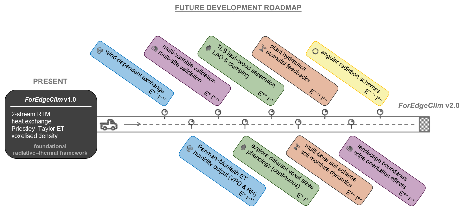
Figure 10 Conceptual development roadmap for the ForEdgeClim radiative–thermal core, illustrating the progression from the current model formulation (present) towards a target fully coupled three-dimensional microclimate model. The road visualisation represents a continuous development trajectory along which key model extensions are introduced, including atmospheric coupling (blue), improved boundary conditions and validation (purple), canopy structure refinement (green), soil–plant interactions (brown), and advanced radiation schemes (yellow). For each extension, the expected implementation effort (E) and potential model impact (I) are indicated using a qualitative rating, where the number of symbols (°) reflects relative magnitude (e.g., E° denotes low effort, I°°° denotes high impact).

6.6 Structural data requirements and scaling

The implementation of ForEdgeClim in this study relied on terrestrial laser scanning (TLS) data, which provide high-resolution 3D representations of forest structure and are therefore well suited for voxel-based microclimate modelling. TLS enables explicit representation of fine-scale variation in canopy density and understorey structure, which is particularly important for resolving lateral radiative transfer and edge-driven temperature gradients (Calders et al., 2020). However, TLS data are subject to occlusion effects and require aggregation during voxelisation, which inevitably smooths sub-voxel structural heterogeneity.

When applying ForEdgeClim with alternative structural data sources, such as UAV-based laser scanning (UAV-LS) or airborne laser scanning (ALS), additional considerations arise. These data typically have coarser spatial resolution and reduced sensitivity to understorey structure, resulting in more vertically aggregated canopy representations (Brede et al., 2019; Calders et al., 2020). Moreover, ALS data have been shown to incompletely detect individual trees, particularly in dense or structurally complex understorey layers, further limiting the representation of fin-scale forest structure (Cao et al., 2023). Consequently, simulations driven by UAV-LS or ALS data are expected to capture broader-scale microclimate patterns but may underestimate fine-scale temperature variability, particularly near forest edges, canopy gaps, or within structurally heterogeneous stands. Users should therefore select voxel resolution and model parameterisation in accordance with the spatial resolution and information content of the available structural data, and interpret model output at scales consistent with those inputs. Future work could explicitly assess how the resolution and type of structural input data influence simulated microclimate patterns, enabling scale-aware application of ForEdgeClim across diverse forest monitoring platforms.

6.7 Ecological relevance and synthesis

From an ecological perspective, the ability to explicitly simulate fine-scale, metre-scale microclimate gradients driven by forest structure and edge proximity is particularly relevant for assessing microclimate buffering and thermal refugia in fragmented landscapes, as well as in forests affected by disturbances that create internal edges (e.g., bark beetle outbreaks or drought-related mortality), which can be represented in ForEdgeClim by modifying the structural input to reflect tree loss or canopy thinning. Fine-scale temperature heterogeneity strongly influences species persistence, phenology, and stress exposure, especially for ectotherms and understorey organisms that operate close to physiological thermal limits (Ford et al., 2013; Vives-Ingla et al., 2023). By resolving temperature patterns arising from both vertical and lateral forest processes, ForEdgeClim provides a mechanistic basis for linking forest management, fragmentation, and biodiversity responses under climate change.

Overall, the results support a growing body of evidence that microclimate buffering is a fundamentally 3D process governed by both vertical and horizontal energy exchanges (Zellweger et al., 2019; De Frenne et al., 2021). By explicitly accounting for these processes, ForEdgeClim enhances our ability to predict habitat-scale thermal heterogeneity and microrefugia in fragmented forest landscapes. Future developments will prioritise the inclusion of wind-driven processes, the inclusion of Penman–Monteith evapotranspiration, a more detailed representation of soil heat fluxes, and coupling with advanced radiative transfer engines such as Eradiate (The Eradiate team, 2025) to enable spectrally resolved simulations. In doing so, ForEdgeClim represents a new generation of process-based microclimate models that combine physical consistency, structural realism, and computational efficiency – offering a flexible platform for further advancing our understanding of forest-climate interactions across scales.

7 Conclusions

ForEdgeClim demonstrates that forest microclimate temperatures can be realistically simulated at high spatial resolution using a voxel-based radiative–thermal framework that explicitly represents vertical and lateral radiative and thermal exchanges, while parameterising turbulent and wind-driven processes implicitly. The model successfully reproduces observed edge-to-core temperature gradients and highlights the central role of lateral energy fluxes in shaping forest microclimate dynamics. Sensitivity analyses indicate that heat-transfer processes exert the strongest control on simulated air temperature patterns, while radiative processes become increasingly important for forest surface temperature and for generating spatial temperature heterogeneity.

Seasonal differences in calibrated parameter values suggest that certain processes, such as phenological changes and seasonal variations in soil moisture, evapotranspiration, and heat storage, are currently simplified or implicitly represented. Nonetheless, the relatively small differences between calibrated and uncalibrated simulations indicate that ForEdgeClim captures the dominant mechanisms governing forest microclimate behaviour under the temperate conditions considered here. This robustness enables the use of a single, annually calibrated parameter set without substantial loss of predictive accuracy, while maintaining realistic spatial and temporal temperature patterns across seasons.

The current formulation of ForEdgeClim captures key drivers of forest microclimate variability under the conditions considered here. The inclusion of further processes, such as wind-driven heat exchange, a Penman–Monteith evapotranspiration scheme, a more detailed representation of soil heat fluxes, and extended radiative transfer schemes, is expected to primarily enhance process realism, improve model robustness under extreme climatic conditions, and increase transferability across forest types, structural configurations, and climatic regions.

By combining high-resolution structural data with a physically grounded, yet computationally efficient framework, ForEdgeClim bridges the gap between simplified empirical microclimate models and computationally intensive ray-tracing approaches. This work underscores the importance of explicitly accounting for lateral energy exchanges when modelling forest edge environments and offers a flexible platform for advancing the development of next-generation process-based microclimate models. By resolving these lateral fluxes at metre-scale resolution, ForEdgeClim extends beyond approaches that assume purely vertical energy exchange and opens new opportunities for ecological applications, including biodiversity studies, species distribution modelling, and assessments of forest resilience under climate change.

Appendix A: Radiative transfer model of ForEdgeClim

A1 Introduction

The radiative transfer model (RTM) used in ForEdgeClim is based on the two-stream RTM implemented in the Ecosystem Demography model (ED) v2.2 (Longo et al., 2019). The ED2.2 two-stream scheme is a generalisation of the two-layer, two-stream radiative transfer model from the Community Land Model (CLM) v4.5 (Oleson et al., 2013), which itself builds on the formulation by Sellers (1985). Although ED2.2 is written entirely in Fortran, an R implementation of its two-stream RTM also exists: the RRTM package, available on GitHub (Shiklomanov, 2023). The development of the two-stream RTM in ForEdgeClim was strongly inspired by this R version.

The two-stream approach represents canopy radiative transfer using two counter-propagating fluxes – upward and downward – thereby capturing the key processes of absorption, reflection, and transmission while remaining computationally efficient. It is widely used in vegetation, land-surface, and climate models because it strikes a practical balance between physical realism and computational cost. The method does, however, simplify angular and spectral complexity and depends heavily on parameterisation. Nevertheless, for applications involving large-scale or iterative simulations – such as in ForEdgeClim – the two-stream formulation provides an appropriate and efficient choice.

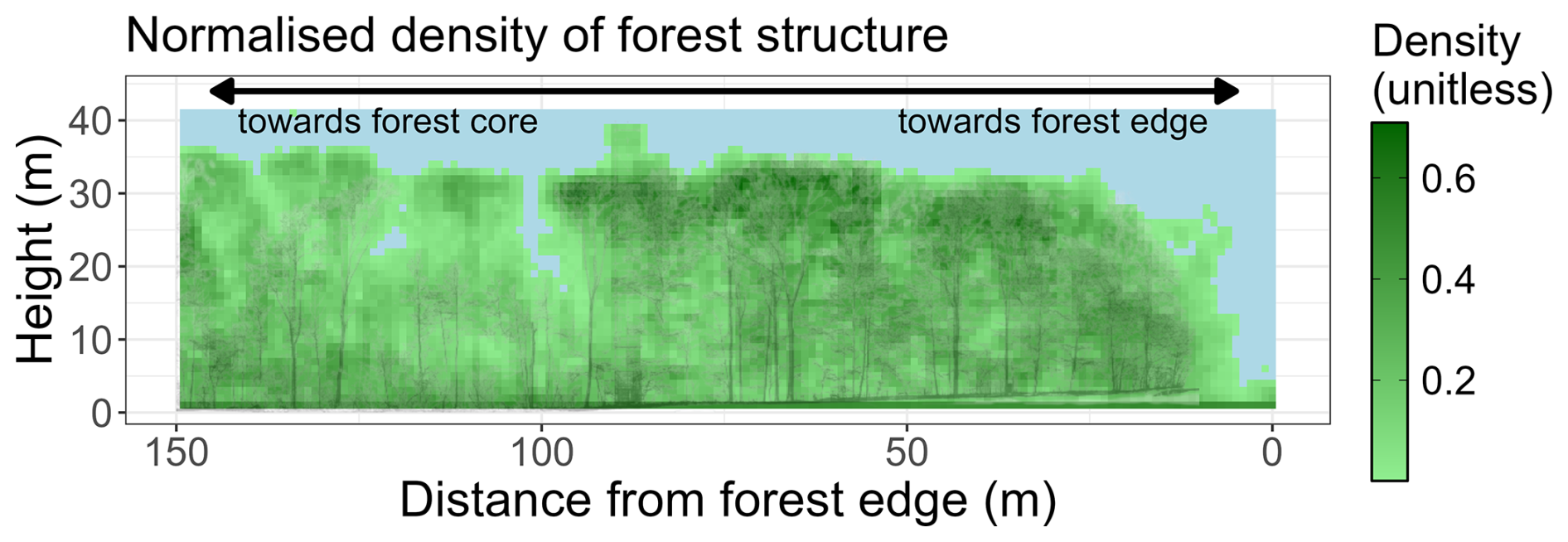
Figure A1 2D visualisation of forest structure as used as structural input data in ForEdgeClim. In this 2D representation, we averaged over the (30) slices perpendicular to the transect direction. The background shows a slice of the central TLS transect line, illustrating the forest structure point cloud.

A2 Forest structure in ForEdgeClim

In ForEdgeClim, forest structure is represented in three dimensions at high spatial resolution, e.g., using 1 m³ voxels, each assigned a density value (ρ) between 0 and 1 derived from, e.g., terrestrial laser scanning (TLS) data. The two-stream RTM is applied to every vertical column and horizontal row of the voxel grid, reflecting the fact that radiation enters the forest both from above (vertical direction) and from the forest edge (horizontal direction). An example of such a voxelised forest transect – from forest edge to forest core – is shown in Fig. A1. This transect was obtained through TLS measurements conducted in July 2023 in the temperate Aelmoeseneiebos forest in Gontrode, Belgium.

A3 Radiative transfer

In this appendix we proceed as follows. First, we summarise the conceptual basis of the two-stream approach. Second, we derive the governing differential equations. Third, we show how these equations allow analytical solutions at the layer scale and how they can be rewritten in matrix form. Finally, we describe how the formulation is parameterised in ForEdgeClim.

In ForEdgeClim, the two-stream approach is used for both shortwave and longwave radiative transfer. Below, we focus on the shortwave RTM; the longwave formulation is analogous, except that it contains no direct-beam component and includes thermal emission from forest surfaces.

In the shortwave RTM, both diffuse irradiance ($I_{\text{sky}}^{\downarrow }$) and direct-beam irradiance ($I_{\text{sky,b}}^{\downarrow }$) enter the canopy from above and from the forest edge. The model then resolves the vertical and horizontal radiation fields as a function of canopy structure and incoming solar radiation.

Direct-beam radiation is represented using an exponential attenuation (Beer–Lambert-type) process (see boxed derivation below), while the diffuse (isotropic) radiation field is obtained by solving a coupled system of linear ordinary differential equations. The solution of this system yields the distribution of light intensity across the discrete canopy layers. This discrete, layer-by-layer formulation approximates the original differential equations, which can be solved efficiently using linear algebra. The full derivation of the differential equations is presented in the following section, Sect. A3.1.

A3.1 Derivation of the two-stream RTM differential equations

The differential equations we aim to derive are clearly explained in Shiklomanov et al. (2021), where they are presented as Eqs. (1) and (2). In this appendix, they are given by Eqs. (A5) and (A6). It was these authors who translated the two-stream ED2.2 RTM into an R implementation (Shiklomanov, 2023). Ultimately, in Sect. A3.2, we discretise these equations and reformulate them as a linear system expressed in matrix form, which is solved using a direct matrix solver.

To begin the derivation, we first introduce the notation for the variables and parameters used throughout the process. These symbols are listed in Table A1.

Table A1 Symbols used in deriving the two-stream RTM differential equations.

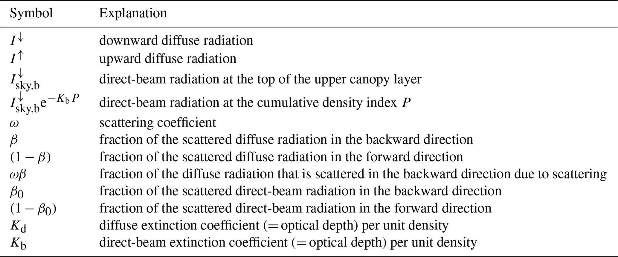
We begin by considering the downward diffuse radiation I^↓, the upward diffuse radiation I^↑, and the direct-beam radiation $I_{\mathrm{b}}^{\downarrow }\left(P\right)$ at a canopy layer characterised by a cumulative density index P. The radiative interactions within and surrounding this layer (shown as olive-green rectangles) are illustrated in Fig. A2.

Focusing first on the downward diffuse radiation I^↓ (Fig. A2a), an amount ${\text{INT}}^{\downarrow }=K_{\mathrm{d}}{I}^{\downarrow }$ is intercepted, where K_d is the diffuse extinction coefficient. The remaining fraction, $(\mathrm{1}-K_{\mathrm{d}})I^{\downarrow }$, passes through the layer without interacting with leaves or woody elements.

Of the intercepted flux, a fraction βωK_dI^↓ is backscattered, $(\mathrm{1}-\mathit{\beta })\mathit{\omega }{K}_{\mathrm{d}}{I}^{\downarrow }$ is scattered forward, and $(\mathrm{1}-\mathit{\omega })K_{\mathrm{d}}{I}^{\downarrow }$ is absorbed. Here, (1−ω) represents the absorption coefficient a. Assuming conservation of energy, the absorption coefficient (a), reflection coefficient (R), and transmission coefficient (T) satisfy:

$$a+R+T=\mathrm{1}.$$

The interactions for the upward diffuse radiation I^↑ and the direct-beam radiation $I_{\mathrm{b}}^{\downarrow }\left(P\right)$ follow analogously. Note that once the direct-beam is intercepted, it is or absorbed or converted to diffuse radiation (${\text{INT}}_{\mathrm{b}}^{\downarrow }=K_{\mathrm{b}}{I}_{\text{sky,b}}^{\downarrow }{\mathrm{e}}^{-K_{\mathrm{b}}P}$) where K_b is the direct-beam extinction coefficient and P is the cumulative density index at the layer. Only the portion of the direct-beam that fully penetrates the layer remains as direct-beam radiation ($(\mathrm{1}-K_{\mathrm{b}})I_{\text{sky,b}}^{\downarrow }{\mathrm{e}}^{-K_{\mathrm{b}}P}$).

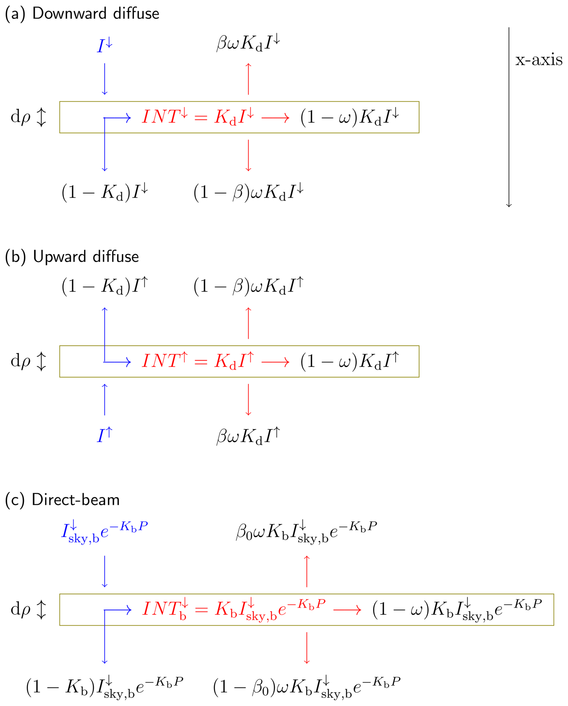
Figure A2 Schematic overview of the downward diffuse (a), upward diffuse (b), and direct-beam (c) components in the two-stream RTM of ForEdgeClim. Blue denotes incoming radiation at the forest layer, whereas red denotes the intercepted radiation.

From the schematics in Fig. A2, taking the three radiation components into account, we can see how the diffuse radiation components change as they pass through a canopy layer along the positive x-direction:

$$\begin{array}{rl}{\displaystyle }{I}^{\downarrow }& {\displaystyle }⟶(\mathrm{1}-K_{\mathrm{d}})I^{\downarrow }+(\mathrm{1}-\mathit{\beta })\mathit{\omega }{K}_{\mathrm{d}}{I}^{\downarrow }+\mathit{\beta }\mathit{\omega }{K}_{\mathrm{d}}{I}^{\uparrow }\\ {\displaystyle }& {\displaystyle }+(\mathrm{1}-{\mathit{\beta }}_{\mathrm{0}})\mathit{\omega }{K}_{\mathrm{b}}{I}_{\text{sky,b}}^{\downarrow }{\mathrm{e}}^{-K_{\mathrm{b}}P},\\ {\displaystyle }{I}^{\uparrow }& {\displaystyle }⟶(\mathrm{1}-K_{\mathrm{d}})I^{\uparrow }+(\mathrm{1}-\mathit{\beta })\mathit{\omega }{K}_{\mathrm{d}}{I}^{\uparrow }+\mathit{\beta }\mathit{\omega }{K}_{\mathrm{d}}{I}^{\downarrow }\\ {\displaystyle }& {\displaystyle }+{\mathit{\beta }}_{\mathrm{0}}\mathit{\omega }{K}_{\mathrm{b}}{I}_{\text{sky,b}}^{\downarrow }{\mathrm{e}}^{-K_{\mathrm{b}}P}.\end{array}$$

Note that in ForEdgeClim the independent variable is the cumulative density index P, rather than geometric depth. Therefore, in the equations below we express derivatives with respect to ρ (or P) instead of x. This leads to the following differential equations for the downward and upward diffuse radiation, expressed along the orientation of the x axis:

$$\begin{array}{}\text{(A1)}& {\displaystyle }{\displaystyle }\begin{array}{rl}{\displaystyle \frac{\mathrm{d}{I}^{\downarrow }}{\mathrm{d}\mathit{\rho }}}& {\displaystyle }=-K_{\mathrm{d}}{I}^{\downarrow }+(\mathrm{1}-\mathit{\beta })\mathit{\omega }{K}_{\mathrm{d}}{I}^{\downarrow }+\mathit{\beta }\mathit{\omega }{K}_{\mathrm{d}}{I}^{\uparrow }\\ {\displaystyle }& {\displaystyle }+(\mathrm{1}-{\mathit{\beta }}_{\mathrm{0}})\mathit{\omega }{K}_{\mathrm{b}}{I}_{\text{sky,b}}^{\downarrow }{\mathrm{e}}^{-K_{\mathrm{b}}P},\end{array}\end{array}$$

$$\begin{array}{}\text{(A2)}& {\displaystyle }\begin{array}{rl}{\displaystyle }-{\displaystyle \frac{\mathrm{d}{I}^{\uparrow }}{\mathrm{d}\mathit{\rho }}}& {\displaystyle }=-K_{\mathrm{d}}{I}^{\uparrow }+(\mathrm{1}-\mathit{\beta })\mathit{\omega }{K}_{\mathrm{d}}{I}^{\uparrow }+\mathit{\beta }\mathit{\omega }{K}_{\mathrm{d}}{I}^{\downarrow }\\ {\displaystyle }& {\displaystyle }+{\mathit{\beta }}_{\mathrm{0}}\mathit{\omega }{K}_{\mathrm{b}}{I}_{\text{sky,b}}^{\downarrow }{\mathrm{e}}^{-K_{\mathrm{b}}P}.\end{array}\end{array}$$

The minus sign in Eq. (A2) originates from the opposite orientation of the upward flux relative to the x axis.

We can simplify Eqs. (A1) and (A2) to obtain:

$$\begin{array}{}\text{(A3)}& {\displaystyle }& {\displaystyle }\begin{array}{rl}{\displaystyle \frac{\mathrm{d}{I}^{\downarrow }}{\mathrm{d}\mathit{\rho }}}& {\displaystyle }=-\left[\mathrm{1}-(\mathrm{1}-\mathit{\beta })\mathit{\omega }\right]K_{\mathrm{d}}{I}^{\downarrow }+\mathit{\beta }\mathit{\omega }{K}_{\mathrm{d}}{I}^{\uparrow }\\ {\displaystyle }& {\displaystyle }+(\mathrm{1}-{\mathit{\beta }}_{\mathrm{0}})\mathit{\omega }{K}_{\mathrm{b}}{I}_{\text{sky,b}}^{\downarrow }{\mathrm{e}}^{-K_{\mathrm{b}}P},\end{array}\text{(A4)}& {\displaystyle }& {\displaystyle }\begin{array}{rl}{\displaystyle \frac{\mathrm{d}{I}^{\uparrow }}{\mathrm{d}\mathit{\rho }}}& {\displaystyle }=\left[\mathrm{1}-(\mathrm{1}-\mathit{\beta })\mathit{\omega }\right]K_{\mathrm{d}}{I}^{\uparrow }-\mathit{\beta }\mathit{\omega }{K}_{\mathrm{d}}{I}^{\downarrow }\\ {\displaystyle }& {\displaystyle }-{\mathit{\beta }}_{\mathrm{0}}\mathit{\omega }{K}_{\mathrm{b}}{I}_{\text{sky,b}}^{\downarrow }{\mathrm{e}}^{-K_{\mathrm{b}}P}.\end{array}\end{array}$$

Equations (A3) and (A4) are mathematically identical to Eqs. (1) and (2) in Shiklomanov et al. (2021), though different notation is used. Table A2 provides the correspondence between the symbols used in this appendix and those in Shiklomanov et al. (2021).

Table A2 Symbol conversion between Shiklomanov et al. (2021) (Shik.) and this appendix (App.).

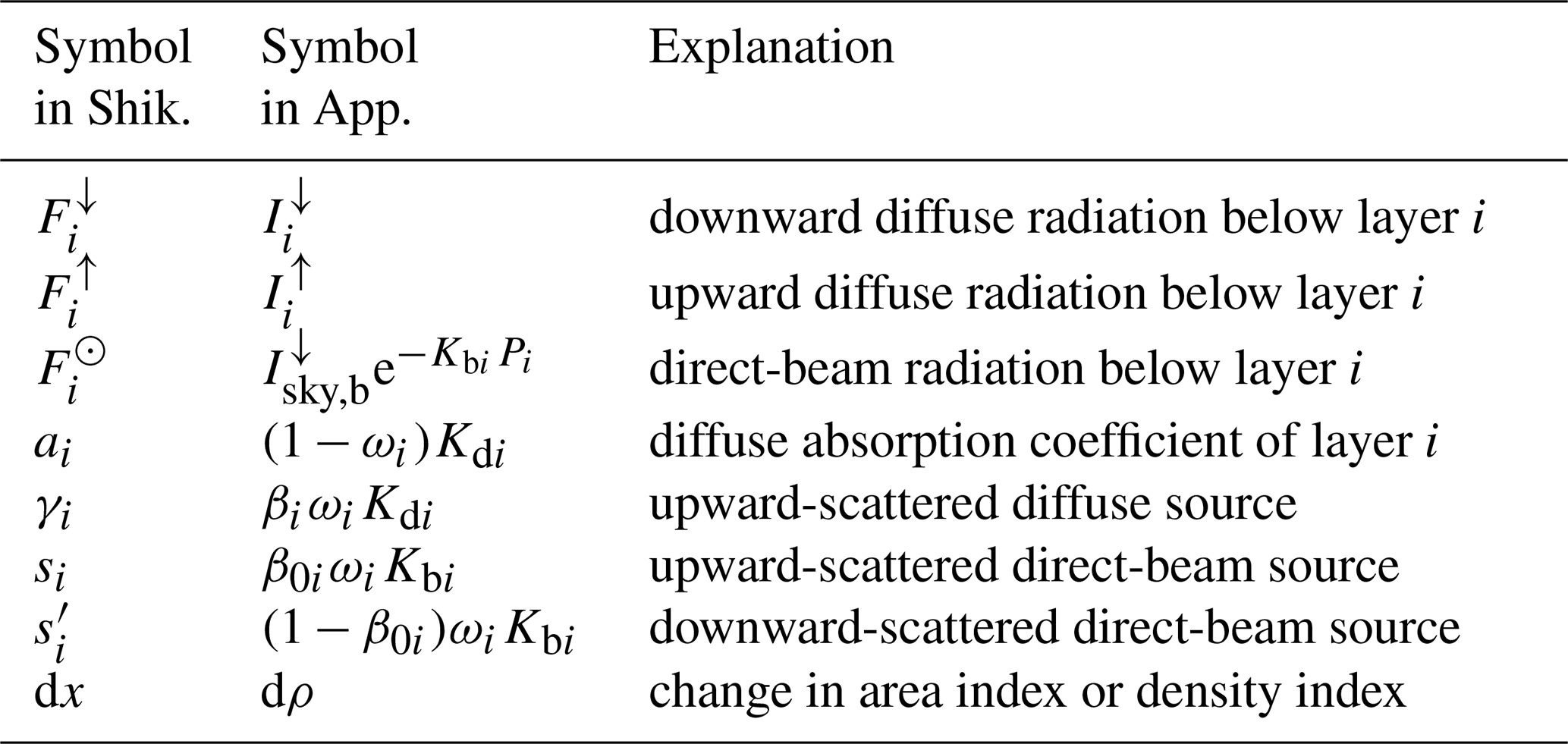
Using the notations from Table A2, Eqs. (A3) and (A4) can be rewritten to express the radiation below layer i as:

$$\begin{array}{}\text{(A5)}& {\displaystyle \frac{\mathrm{d}{F}_i^{\downarrow }}{\mathrm{d}x}}& {\displaystyle }=-(a_i+{\mathit{\gamma }}_i)F_i^{\downarrow }+{\mathit{\gamma }}_i{F}_i^{\uparrow }+s_i^{\prime }{F}_i^{\odot },\text{(A6)}& {\displaystyle }-{\displaystyle \frac{\mathrm{d}{F}_i^{\uparrow }}{\mathrm{d}x}}& {\displaystyle }=-(a_i+{\mathit{\gamma }}_i)F_i^{\uparrow }+{\mathit{\gamma }}_i{F}_i^{\downarrow }+s_i{F}_i^{\odot }.\end{array}$$

These equations are exactly equivalent to those presented in Shiklomanov et al. (2021).

Throughout this derivation, we used Chapter 14 of Gordon Bonan's Climate Change and Terrestrial Ecosystem Modeling as background material, which proved helpful for understanding how Eqs. (A3) and (A4) are formulated (Bonan, 2019).

A3.2 Solving the two-stream RTM differential equations

To solve the differential equations, we rely on the work of Shiklomanov et al. (2021). These authors explain that their formulations in Eqs. (A5) and (A6) are solved, based on the analytical solutions derived in ED2.2. A detailed description of how these analytical solutions are obtained is provided in Sect. S12 of Longo et al. (2019).

Briefly summarising the procedure: the derivatives of Eqs. (A5) and (A6) are taken to obtain expressions for the second derivatives. The first derivatives are then substituted into these expressions, which yields two independent second-order ordinary differential equations. Each equation has an analytical solution composed of a homogeneous and a particular component. The homogeneous solution represents the intrinsic exponential attenuation and scattering behaviour of the radiation field when all source terms are set to zero, whereas the particular solution captures the constant forcing introduced by direct and diffuse radiation sources.

Building on this framework, and using the definitions $K_{\mathrm{d}i}=\frac{\mathrm{1}}{{\stackrel{\mathrm{‾}}{\mathit{\mu }}}_i}$ and $K_{\mathrm{b}i}=\frac{\mathrm{1}}{{\mathit{\mu }}_i^{\odot }}$ – where the μ values are the inverse of the optical depth per unit density index – we can write Eqs. (A5) and (A6) in their analytical form as:

$$\begin{array}{}\text{(A7)}& {\displaystyle }& {\displaystyle }{\displaystyle }{F}_i^{\downarrow }{\displaystyle }=x_{(\mathrm{2}i-\mathrm{1})}{\mathit{\gamma }}_i^{+}\cdot {\mathrm{e}}^{-{\mathit{\lambda }}_i{P}_i}+x_{\left(\mathrm{2}i\right)}{\mathit{\gamma }}_i^{-}\cdot {\mathrm{e}}^{+{\mathit{\lambda }}_i{P}_i}+{\mathit{\delta }}_i^{+}\cdot {\mathrm{e}}^{\frac{-P_i}{{\mathit{\mu }}_i^{\odot }}},\text{(A8)}& {\displaystyle }& {\displaystyle }{\displaystyle }{F}_i^{\uparrow }{\displaystyle }=x_{(\mathrm{2}i-\mathrm{1})}{\mathit{\gamma }}_i^{-}\cdot {\mathrm{e}}^{-{\mathit{\lambda }}_i{P}_i}+x_{\left(\mathrm{2}i\right)}{\mathit{\gamma }}_i^{+}\cdot {\mathrm{e}}^{+{\mathit{\lambda }}_i{P}_i}+{\mathit{\delta }}_i^{-}\cdot {\mathrm{e}}^{\frac{-P_i}{{\mathit{\mu }}_i^{\odot }}}.\end{array}$$

In Eqs. (A7) and (A8), x is a vector with layer specific unknowns and ${\mathit{\gamma }}_i^{\pm }$, ${\mathit{\delta }}_i^{\pm }$ and λ_i are defined as:

$$\begin{array}{ll}{\displaystyle }& {\displaystyle }{\mathit{\gamma }}_i^{\pm }={\displaystyle \frac{\mathrm{1}}{\mathrm{2}}}(\mathrm{1}\pm \sqrt{{\displaystyle \frac{\mathrm{1}-{\mathit{\omega }}_i}{\mathrm{1}-(\mathrm{1}-\mathrm{2}{\mathit{\beta }}_i){\mathit{\omega }}_i}}}),\\ {\displaystyle }& {\displaystyle }{\mathit{\delta }}_i^{\pm }={\displaystyle \frac{({\mathit{\kappa }}_i^{+}\pm {\mathit{\kappa }}_i^{-}){{\mathit{\mu }}_i^{\odot }}^{\mathrm{2}}}{\mathrm{2}(\mathrm{1}-{\mathit{\lambda }}_i^{\mathrm{2}}{{\mathit{\mu }}_i^{\odot }}^{\mathrm{2}})}},\\ {\displaystyle }& {\displaystyle }{\mathit{\lambda }}_i^{\mathrm{2}}={\displaystyle \frac{[\mathrm{1}-(\mathrm{1}-\mathrm{2}{\mathit{\beta }}_i\left){\mathit{\omega }}_i\right](\mathrm{1}-{\mathit{\omega }}_i)}{{{\stackrel{\mathrm{‾}}{\mathit{\mu }}}_i}^{\mathrm{2}}}}.\end{array}$$

And in the equations for ${\mathit{\delta }}_i^{\pm }$, ${\mathit{\kappa }}_i^{\pm }$ are defined as:

$$\begin{array}{ll}{\displaystyle }& {\displaystyle }{\mathit{\kappa }}_i^{+}=-\left[{\displaystyle \frac{\mathrm{1}-(\mathrm{1}-\mathrm{2}{\mathit{\beta }}_i){\mathit{\omega }}_i}{{\stackrel{\mathrm{‾}}{\mathit{\mu }}}_i}}+{\displaystyle \frac{\mathrm{1}-\mathrm{2}{\mathit{\beta }}_{\mathrm{0}i}}{{\mathit{\mu }}_i^{\odot }}}\right]{\displaystyle \frac{{\mathit{\omega }}_i{F}_{i+\mathrm{1}}^{\odot }}{{\mathit{\mu }}_i^{\odot }}},\\ {\displaystyle }& {\displaystyle }{\mathit{\kappa }}_i^{-}=-\left[{\displaystyle \frac{(\mathrm{1}-\mathrm{2}{\mathit{\beta }}_{\mathrm{0}i})(\mathrm{1}-{\mathit{\omega }}_i)}{{\stackrel{\mathrm{‾}}{\mathit{\mu }}}_i}}+{\displaystyle \frac{\mathrm{1}}{{\mathit{\mu }}_i^{\odot }}}\right]{\displaystyle \frac{{\mathit{\omega }}_i{F}_{i+\mathrm{1}}^{\odot }}{{\mathit{\mu }}_i^{\odot }}}.\end{array}$$

For n layers, the full diffuse canopy radiation profile is defined by a vector of size 2n+2 with $F_i^{\downarrow }$ and $F_i^{\uparrow }$ radiation fluxes for every interface immediately below layer i. Table A3 shows what this means for the canopy top and ground fluxes.

Table A3 Symbols for canopy top and ground fluxes.

Table A4 Boundary conditions at the canopy top.

Equations (A7) and (A8) can be rewritten in matrix format to solve for x_i:

$$\begin{array}{}\text{(A9)}& \mathbf{\text{S}}\mathit{x}=\mathit{y}\end{array}$$

with $\mathbf{\text{S}}\mathrm{a}(\mathrm{2}n+\mathrm{2})\times (\mathrm{2}n+\mathrm{2})$ pentadiagonal matrix and

$$\begin{array}{rl}{\displaystyle }& {\displaystyle }\mathit{x}=(x_{\mathrm{1}},x_{\mathrm{2}},\mathrm{\dots },x_{\mathrm{2}n+\mathrm{1}},x_{\mathrm{2}n+\mathrm{2}}),\\ {\displaystyle }& {\displaystyle }\mathit{y}=(y_{\mathrm{1}},y_{\mathrm{2}},\mathrm{\dots },y_{\mathrm{2}n+\mathrm{1}},y_{\mathrm{2}n+\mathrm{2}}).\end{array}$$

The elements of S take the following format:

$$\begin{array}{rl}{\displaystyle }& {\displaystyle }{S}_{\mathrm{1},\mathrm{1}}=({\mathit{\gamma }}_{\mathrm{1}}^{-}-{\mathit{\omega }}_{\mathrm{g}}{\mathit{\gamma }}_{\mathrm{1}}^{+})\cdot {\mathrm{e}}^{-{\mathit{\lambda }}_{\mathrm{1}}{P}_{\mathrm{1}}},\\ {\displaystyle }& {\displaystyle }{S}_{\mathrm{1},\mathrm{2}}=({\mathit{\gamma }}_{\mathrm{1}}^{+}-{\mathit{\omega }}_{\mathrm{g}}{\mathit{\gamma }}_{\mathrm{1}}^{-})\cdot {\mathrm{e}}^{+{\mathit{\lambda }}_{\mathrm{1}}{P}_{\mathrm{1}}},\\ {\displaystyle }& {\displaystyle }{S}_{\mathrm{2}i,\mathrm{2}i-\mathrm{1}}={\mathit{\gamma }}_i^{+},\\ {\displaystyle }& {\displaystyle }{S}_{\mathrm{2}i,\mathrm{2}i}={\mathit{\gamma }}_i^{-},\\ {\displaystyle }& {\displaystyle }{S}_{\mathrm{2}i,\mathrm{2}i+\mathrm{1}}=-{\mathit{\gamma }}_{i+\mathrm{1}}^{+}\cdot {\mathrm{e}}^{-{\mathit{\lambda }}_{i+\mathrm{1}}{P}_{i+\mathrm{1}}},\\ {\displaystyle }& {\displaystyle }{S}_{\mathrm{2}i,\mathrm{2}i+\mathrm{2}}=-{\mathit{\gamma }}_{i+\mathrm{1}}^{-}\cdot {\mathrm{e}}^{+{\mathit{\lambda }}_{i+\mathrm{1}}{P}_{i+\mathrm{1}}},\\ {\displaystyle }& {\displaystyle }{S}_{\mathrm{2}i+\mathrm{1},\mathrm{2}i-\mathrm{1}}={\mathit{\gamma }}_i^{-},\\ {\displaystyle }& {\displaystyle }{S}_{\mathrm{2}i+\mathrm{1},\mathrm{2}i}={\mathit{\gamma }}_i^{+},\\ {\displaystyle }& {\displaystyle }{S}_{\mathrm{2}i+\mathrm{1},\mathrm{2}i+\mathrm{1}}=-{\mathit{\gamma }}_{i+\mathrm{1}}^{+}\cdot {\mathrm{e}}^{-{\mathit{\lambda }}_{i+\mathrm{1}}{P}_{i+\mathrm{1}}},\\ {\displaystyle }& {\displaystyle }{S}_{\mathrm{2}i+\mathrm{1},\mathrm{2}i+\mathrm{2}}=-{\mathit{\gamma }}_{i+\mathrm{1}}^{-}\cdot {\mathrm{e}}^{+{\mathit{\lambda }}_{i+\mathrm{1}}{P}_{i+\mathrm{1}}},\\ {\displaystyle }& {\displaystyle }{S}_{\mathrm{2}n+\mathrm{2},\mathrm{2}n+\mathrm{1}}={\mathit{\gamma }}_{n+\mathrm{1}}^{+},\\ {\displaystyle }& {\displaystyle }{S}_{\mathrm{2}n+\mathrm{2},\mathrm{2}n+\mathrm{2}}={\mathit{\gamma }}_{n+\mathrm{1}}^{-}.\end{array}$$

And the elements of y are given by:

$$\begin{array}{rl}{\displaystyle }& {\displaystyle }{y}_{\mathrm{1}}={\mathit{\omega }}_{\mathrm{g}}{F}_{\mathrm{1}}^{\odot }-({\mathit{\delta }}_{\mathrm{1}}^{-}-{\mathit{\omega }}_{\mathrm{g}}{\mathit{\delta }}_{\mathrm{1}}^{+})\cdot {\mathrm{e}}^{\frac{-P_{\mathrm{1}}}{{\mathit{\mu }}_{\mathrm{1}}^{\odot }}},\\ {\displaystyle }& {\displaystyle }{y}_{\mathrm{2}i}={\mathit{\delta }}_{i+\mathrm{1}}^{+}\cdot {\mathrm{e}}^{\frac{-P_{i+\mathrm{1}}}{{\mathit{\mu }}_{i+\mathrm{1}}^{\odot }}}-{\mathit{\delta }}_i^{+},\\ {\displaystyle }& {\displaystyle }{y}_{\mathrm{2}i+\mathrm{1}}={\mathit{\delta }}_{i+\mathrm{1}}^{-}\cdot {\mathrm{e}}^{\frac{-P_{i+\mathrm{1}}}{{\mathit{\mu }}_{i+\mathrm{1}}^{\odot }}}-{\mathit{\delta }}_i^{-},\\ {\displaystyle }& {\displaystyle }{y}_{\mathrm{2}n+\mathrm{2}}=F_{\text{sky}}^{\downarrow }-{\mathit{\delta }}_{n+\mathrm{1}}^{+}.\end{array}$$

To obtain the final solution of the matrix equation (Eq. A9), boundary conditions must be specified at the canopy top and at the ground surface. For the ground surface, only the ground scattering coefficient ω₁=ω_g needs to be defined, assuming no ground transmittance and only scattering and absorption. The boundary conditions at the canopy top follow those used in ED2.2 and are listed in Table A4.

A3.3 Parameterisation in ForEdgeClim

We note that the two-stream RTM differential equations (Eqs. A3 and A4) depend on the parameters ω, β, β₀, K_d, and K_b. Within the ForEdgeClim framework, these five parameters are fixed (i.e., parameterised) at the beginning of each model run. This implies that all voxels are assigned the same optical properties; that is, the same five parameter values are used for every voxel i. In ED2.2, layers are considered infinitesimally thin, with each layer representing a cohort with its own optical parameters. In ForEdgeClim, however, layers (i.e., voxels) do have a finite thickness, defined by their voxel density ρ_i. Consequently, the extinction coefficients are scaled by the voxel density ρ_i, such that $K_{\mathrm{b}i}=K_{\mathrm{b}}\cdot {\mathit{\rho }}_i$ and analogously $K_{\mathrm{d}i}=K_{\mathrm{d}}\cdot {\mathit{\rho }}_i$. This all remains a simplification, as upper canopy layers contain more leaves and branches, whereas lower layers contain proportionally more stems. Moreover, the model does not distinguish between tree species: although reflectance and transmittance vary across species, these differences are not represented. An overview of the assumptions and limitations of the ForEdgeClim RTM is given in Table A5.

We do, however, differentiate between the horizontal and vertical directions: the parameters ω, β, β₀, K_d, and K_b take distinct values in each direction. The ground-scattering coefficient ω_g likewise differs between horizontal and vertical transfer. Notably, there is no true 'ground reflection' in the horizontal direction; the scattering defined there represents scattering within the forest interior rather than reflection from the ground surface.

Analogously, the corresponding parameters differ between the shortwave and longwave RTMs. In the longwave case, no direct-beam parameters (β₀ and K_b) are required. Instead, an additional parameter, ϵ_f, the forest emissivity, is introduced to account for thermal emission from forest surfaces.

Table A5 Assumptions and limitations of the two-stream RTM in ForEdgeClim.

A4 Visualisation of the ForEdgeClim RTM

Below are some example output plots of the ForEdgeClim RTM. Figures A3 and A4 respectively show the shortwave and longwave radiation components for the transect in Fig. A1. Here too, the structure of the summer month July 2023 is used. The figures show the light rays at 14:00 UTC.

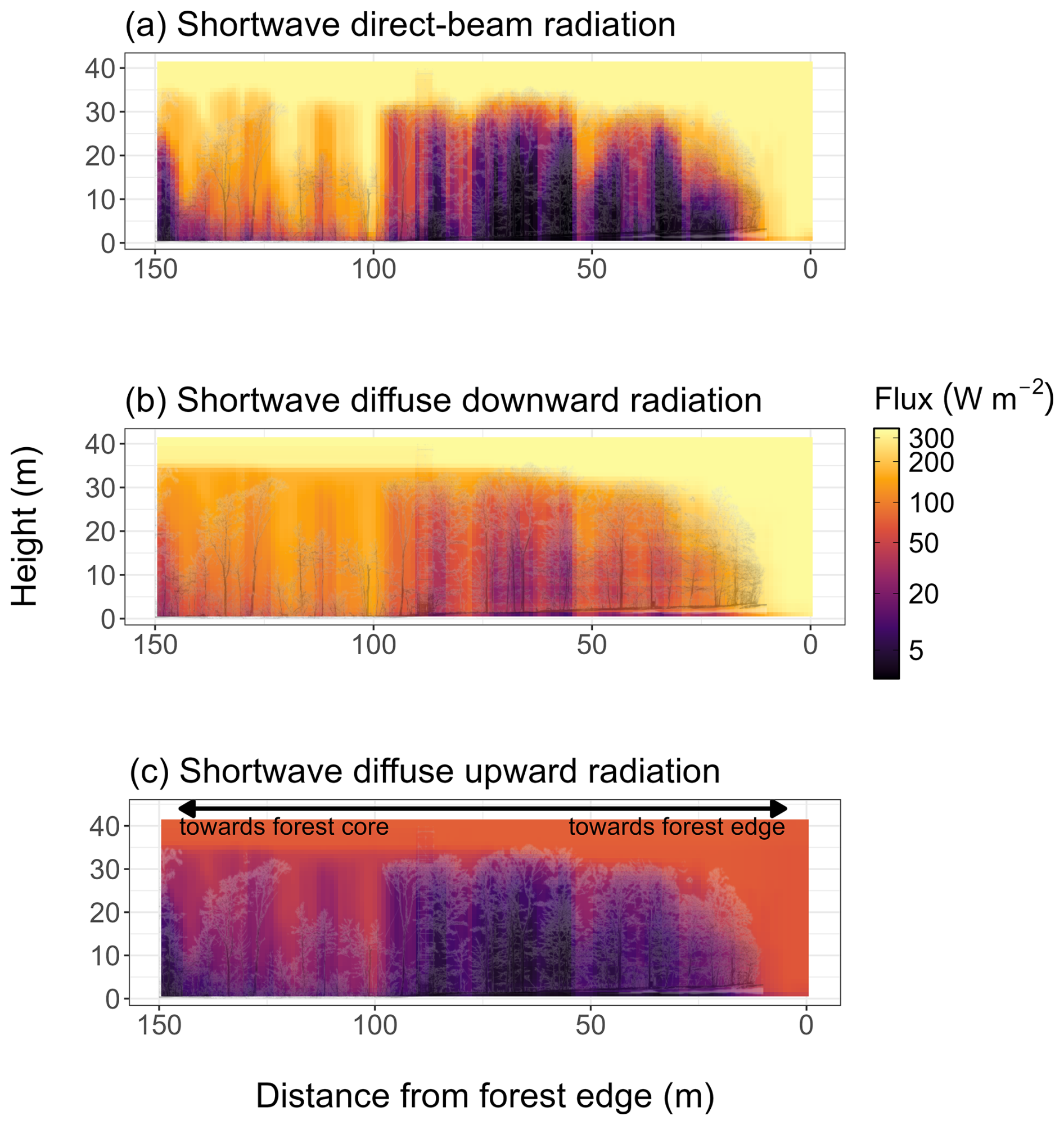
Figure A3 Shortwave radiation components on 8 July 2023 at 14:00 UTC. (a) Direct-beam radiation, (b) diffuse downward radiation, and (c) diffuse upward radiation. In this 2D representation, we averaged over the (30) slices perpendicular to the transect direction. The background shows a slice of the central TLS transect line, illustrating the forest structure point cloud. Colours represent radiation flux using a pseudo-logarithmic colour scale (σ=5), which behaves linearly near zero and logarithmically for higher values.

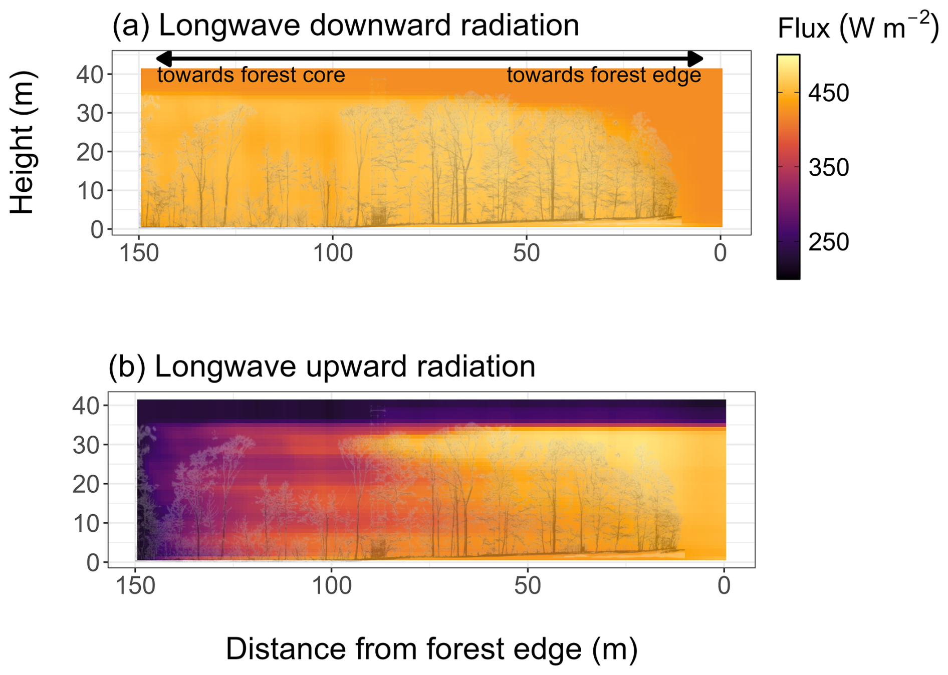
Figure A4 Longwave radiation components on 8 July 2023 at 14:00 UTC. (a) Downward radiation and (b) upward radiation. In this 2D representation, we averaged over the (30) slices perpendicular to the transect direction. The background shows a slice of the central TLS transect line, illustrating the forest structure point cloud.

Appendix B: Tables

Table B1 Model constants. The column submodel indicates the component of the model to which each constant belongs. LW RTM refers to the longwave radiative transfer model, H to the sensible heat flux, and LE to the latent heat flux.

Appendix C: Figures

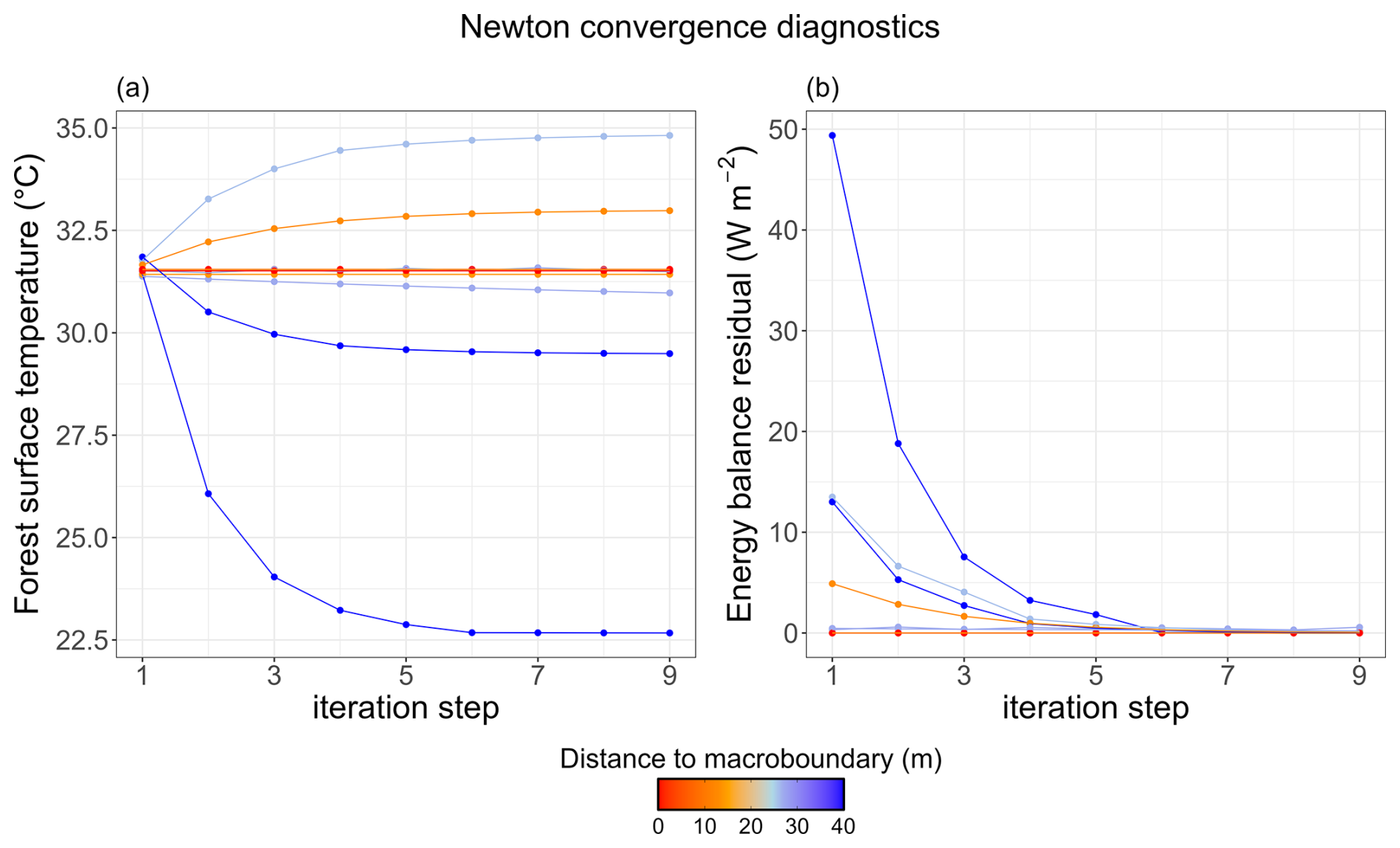
Figure C1 Convergence diagnostics of Newton's method for ten randomly selected voxels on 8 July 2023 at 14:00 UTC for a transect in the temperate Aelmoeseneiebos Forest (Gontrode, Belgium; see Sect. 3 for site details). (a) Convergence behaviour of the forest surface temperature (T_f). Voxels are initially assigned a temperature close to the macroenvironmental air temperature and iteratively relax towards their equilibrium temperature. (b) Convergence of the energy balance residual (E_bal). Some voxels start with a low initial E_bal, whereas others converge towards the prescribed tolerance of $E_{\text{bal}}=\mathrm{2}\mathrm{W}{\mathrm{m}}^{-\mathrm{2}}$. Colours indicate the distance of each voxel from the closed macroenvironment boundary, i.e., canopy top or forest edge.

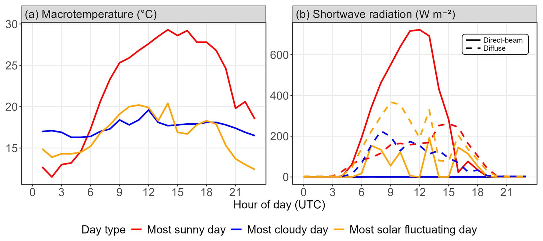
Figure C2 Mean hourly model drivers for three representative calibration days during the summer season. (a) Mean hourly macrotemperature and (b) incoming shortwave radiation. Shortwave radiation is separated into direct-beam and diffuse components. Colours indicate day type: most sunny day (7 July 2023), most cloudy day (31 July 2023), and most solar-fluctuating day (20 July 2023).

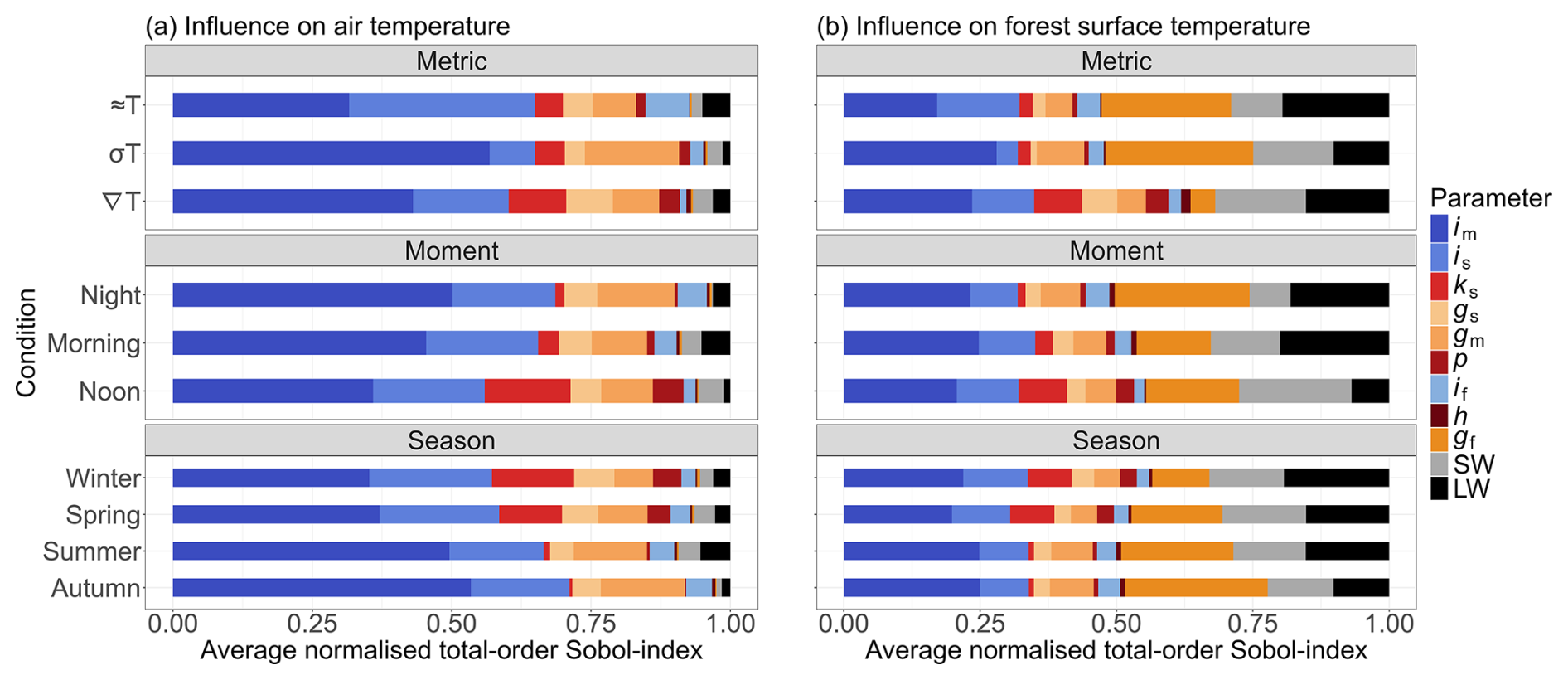
Figure C3 Sobol sensitivity analysis of parameter contributions to (a) air temperature variance and (b) forest surface temperature variance along the vertical transect line. The parameters i_m, i_s and i_f, representing the distances of influence from the macroenvironment, soil surface, and forest surface, respectively, are shown in blue. The parameters g_m, g_s, and g_f, representing convection from the macroenvironment, soil surface, and forest surface, respectively, are shown in orange. The parameters k_s (soil conductance), h (air heat conduction coefficient), and p (fraction of net radiation R_n absorbed by the soil surface) are shown in red. SW refers to all shortwave RTM parameters (nine parameters), and LW to all longwave RTM parameters (seven parameters). ≈T denotes the mean temperature, σT the temperature standard deviation, and ∇T the temperature gradient from forest core to edge. For further details on the model parameters, see Table 1.

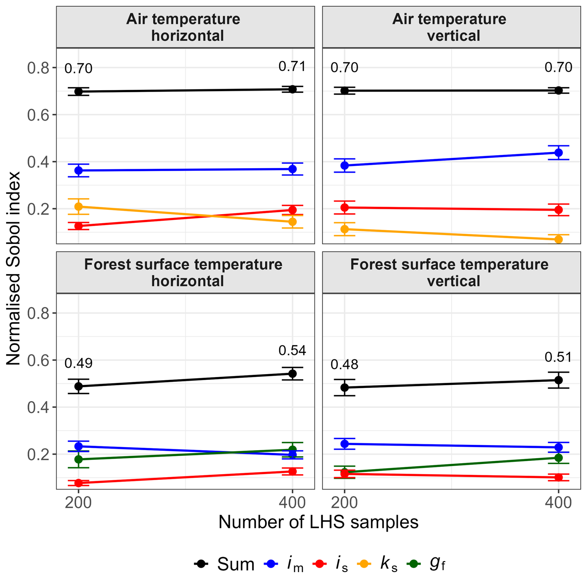
Figure C4 Convergence of Sobol sensitivity indices with increasing sample size. Total-order indices are shown for the most influential parameters for both air temperature (i_m, i_s, and k_s) and forest surface temperature (i_m, i_s, and g_f), as well as their combined contribution (Sum), based on 200 and 400 Latin hypercube samples (LHS). Here, i_m and i_s represent the distance of influence from the macroenvironment and from the soil surface, respectively, k_s denotes soil conductance, and g_f the bulk convection coefficient between air and the forest surface. Values represent averages across all conditions (i.e., seasons, times of day, and metrics) for both air temperature and forest surface temperature, along horizontal and vertical transects. Notably, for air temperature, the combined contribution of the most influential parameters – on which the model calibration is based – remains nearly unchanged when increasing the sample size from 200–400, indicating strong convergence of the key drivers. The stability in both ranking and magnitude further supports the robustness of the sensitivity analysis for parameter screening. Error bars indicate the standard error of the mean Sobol index across all conditions.

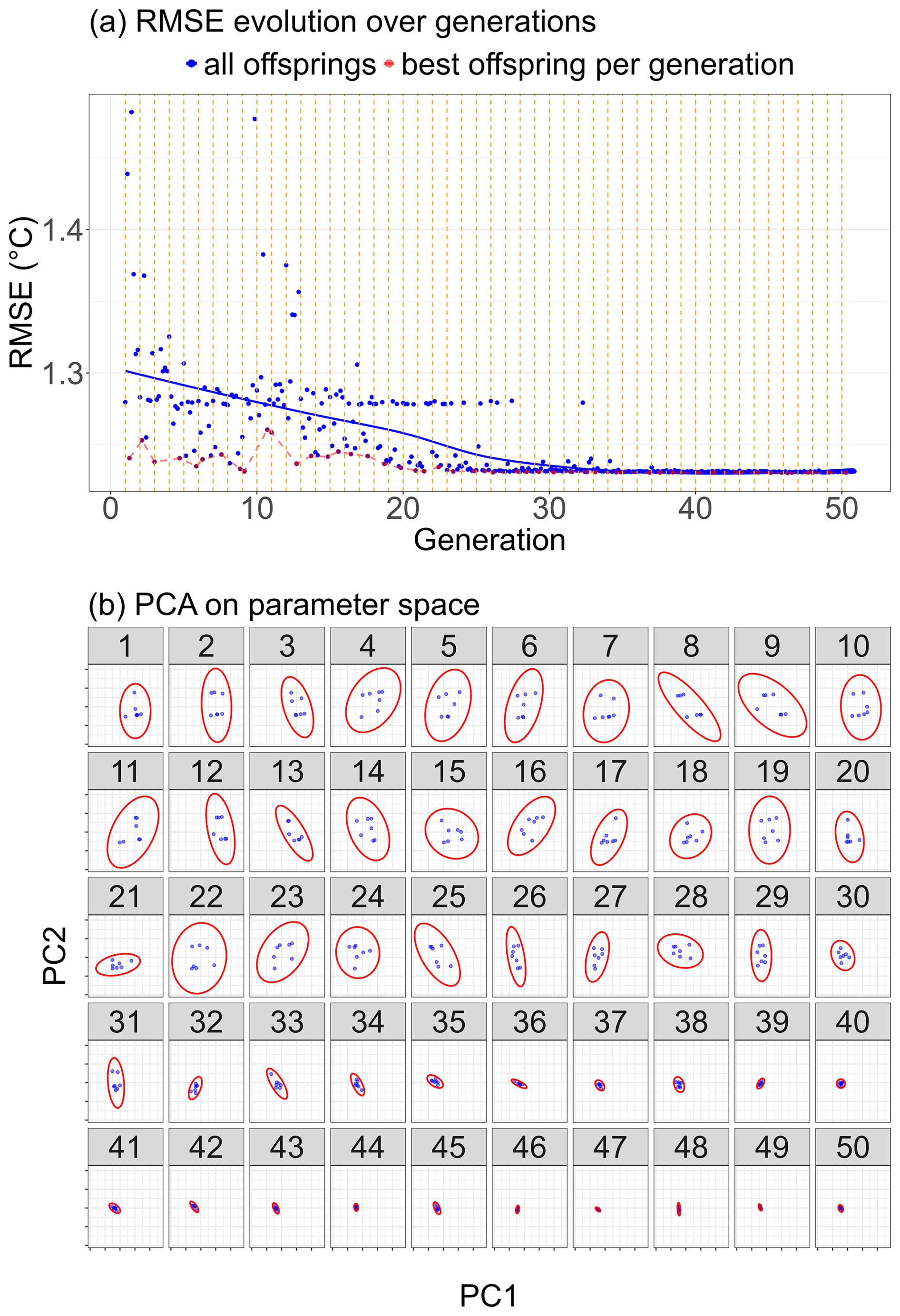
Figure C5 Convergence diagnostics of the CMA-ES algorithm for the summer season. (a) Offspring RMSE between observed and modelled air temperature (blue). The solid blue curve represents a LOESS-smoothed trend. The red dotted line indicates the best RMSE of a certain generation. The orange dotted lines indicate the separation between the different generations. (b) Principal component analysis (PCA) on the parameter space showing CMA-ES parameter spread per generation. The blue dots represent the offsprings and the red ellipse the 95 % spread.

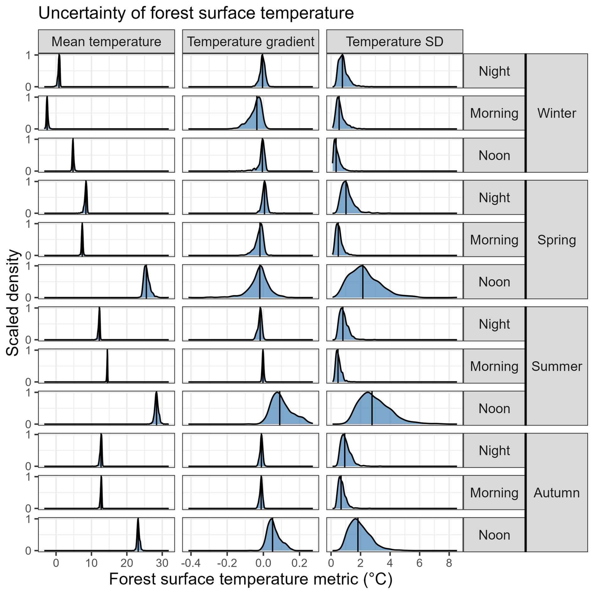
Figure C6 Uncertainty in forest surface temperature along the vertical transect derived from the Sobol parameter ensemble. Density curves are scaled (peaks are set to a value of 1) to facilitate comparison of distribution shapes. Vertical lines indicate median values.