S2AS v1.0 and 2D polarity–volatility lumping framework v1.0: automated compound classification and scalable lumping for organic aerosol modelling

Advancements in near-explicit chemical reaction mechanisms, such as the Master Chemical Mechanism (MCM) or the Generator of Explicit Chemistry and Kinetics of Organics in the Atmosphere (GECKO-A), have enabled highly detailed simulations of atmospheric chemistry. Such simulations offer a bottom-up approach to accompany and inform laboratory chamber experiments of organic aerosol formation or to model the complex chemistry of mixtures of volatile aerosol precursors for specific tropospheric conditions. These chemical reaction mechanisms, while comprehensive, generate hundreds to millions of organic components, creating computational challenges for subsequent applications in multiphase equilibrium gas–particle partitioning models to predict secondary organic aerosol (SOA) mass concentrations, phase compositions, and hygroscopicity. The wealth of simulated reactions and components also requires substantial simplifications for reduced-complexity representations in large-scale atmospheric models. This study introduces a suite of software tools to automate relevant pure-component property predictions as well as a 2-dimensional (2D) polarity–volatility lumping framework to systematically reduce the complexity of chemical mechanism outputs. We introduce a new polarity metric for use in the 2D framework, a ratio of a component's activity coefficients in water and an organic solvent (hexanediol). This ratio is computed using the Aerosol Inorganic–Organic Mixtures Functional groups Activity Coefficients (AIOMFAC) model. The 2D framework offers grid-based and cluster-based methods to select an adjustable number of surrogate species and offers flexibility in the choice of polarity axis. Our methods utilize the Simplified Molecular Input Line Entry System (SMILES) description of molecular structures. A new tool, SMILES to AIOMFAC subgroups (S2AS), is introduced to automatically generate AIOMFAC-model input files and to handle exception cases consistently. We demonstrate the application of our framework using systems of hundreds to thousands of components generated by near-explicit chemical mechanisms. The new framework enables tailored reduced-complexity representations of gas–particle systems.

1 Introduction

Secondary organic aerosol material (SOA) is formed through chemical processing and gas–particle partitioning of volatile organic precursors. SOA can consist of hundreds to millions of distinct kinds of molecules, stemming from biogenic and anthropogenic emission sources (Hallquist et al., 2009; Lannuque et al., 2021). In addition, atmospheric aerosols frequently contain primary organic aerosol material (POA), water and dissolved electrolytes, as well as insoluble species. The complexities in sources, chemical and physical transformations and resulting gas- and particle-phase mixtures, introduces computational challenges when attempting to predict component properties and the partitioning behaviour of such organic–inorganic aerosol systems. Atmospheric chemical transport models often resort to the use of highly simplified volatility binning or approaches relying on surrogate components for gas–particle partitioning predictions of organics. Those models often also assume ideal condensed phase mixing behaviour, in part due to computational time considerations and in part due to a lack of efficient thermodynamic mixing models (Byun et al., 1999; Semeniuk and Dastoor, 2020).

Laboratory experiments, field studies and theory suggest that nonideal mixing in condensed particulate matter (PM) phases impacts the gas–particle partitioning process and influences the physicochemical properties of the condensed phase, often leading to liquid–liquid phase separation over a wide range of environmental conditions (Pankow, 2003; Erdakos and Pankow, 2004; Smith et al., 2011; Bertram et al., 2011; Zuend et al., 2010; Huang et al., 2021; Schervish and Shiraiwa, 2023). Models have been developed to predict SOA formation based on the thermodynamic equilibrium partitioning of semivolatile organic oxidation products, including versions for application in atmospheric large-scale models (Pun et al., 2002; Griffin et al., 2003; Chang and Pankow, 2006; Tulet et al., 2006; Pankow and Chang, 2008; Wang et al., 2022). The model by Griffin et al. (2003) allows for gas–particle equilibrium of organic and inorganic compounds considering an organic and an inorganic phase, but it does not allow organics and salts to partition between the two PM phases. A gas–particle partitioning approach using the activity coefficient model X-UNIFAC proposed by (Chang and Pankow, 2006), an extension of the UNIquac Functional group Activity Coefficients (UNIFAC) model (Fredenslund et al., 1975), enabled equilibrium of all species between all phases present yet restricted to single electrolyte components. Since then, improved thermodynamic multiphase modelling frameworks have been introduced (e.g. Zuend et al., 2010) for applications in box models, yet all such models reach computational limitations, such as excessive memory requirements, when applied to highly complex aerosol systems containing many hundreds to thousands of interacting components.

Based on theory, the equilibrium gas–particle partitioning of a certain semi-volatile (organic) compound is mainly governed by three key properties: (1) the pure-component saturation vapour pressure, (2) the effective activity coefficient in the absorbing aerosol phase and (3) the total mass concentration of all the material in the absorbing condensed phase (e.g., Pankow, 2003; Donahue et al., 2006; Zuend et al., 2010). Thus, the pure-component saturation vapour pressure is a critical input for equilibrium partitioning models, including for box models based on the Aerosol Inorganic–Organic Mixtures Functional group Activity Coefficients (AIOMFAC) model (Zuend et al., 2008, 2011), X-UNIFAC and other UNIFAC variants (Hansen et al., 1991; Pankow and Asher, 2008; Chang and Pankow, 2010; Compernolle et al., 2011).

One way to generate the chemical composition of an air parcel is by predicting the gas- and/or particle-phase composition by means of integrating a chemical reaction scheme over time. In this study, we focus on the development and discussion of necessary tools for handling the output of detailed reaction mechanisms. The aim is to process such output for subsequent equilibrium gas–particle partitioning computations, which in turn predict the composition, PM mass concentration and other SOA properties.

1.1 Near-explicit chemical mechanisms

The Master Chemical Mechanism (MCM, v3.3.1) is a near-explicit reaction scheme of the gas-phase chemistry, covering a substantial set of (volatile) aliphatic and aromatic hydrocarbon compounds in atmospheric chemistry models (Jenkin et al., 1997; Saunders et al., 2003). Oxidation products of volatile or intermediate-volatility compounds may be of sufficiently low volatility to contribute to condensed aerosol mass. In past work, molecular concentrations of a subset of oxidized compounds simulated by MCM have been used as input composition information in the gas–particle partitioning model by Zuend and Seinfeld (2012) to predict SOA mass concentrations at varying levels of relative humidity (RH). Another state-of-the-art, near-explicit model is the Generator for Explicit Chemistry and Kinetics of Organics in the Atmosphere (GECKO-A) by Aumont et al. (2005); Mouchel-Vallon et al. (2020). GECKO-A is a chemical mechanism generator, which automates the creation of thousands of reactions and thousands to millions of oxidation and fragmentation products from a single precursor or a mixture of precursors (depending on the structural complexity of the precursors). GECKO-A achieves this by algorithmically generating the likely chemical products and related kinetic rate constants for multiple generations of reactions of a precursor and its derivatives (Aumont et al., 2005; Mouchel-Vallon et al., 2020). A box model (as part of GECKO-A) can then be run under given conditions of temperature, RH, reaction time and oxidant concentrations to generate the molecular output concentrations at specified times of interest (Aumont et al., 2005; Mouchel-Vallon et al., 2020). The processing of the wealth of component information from such near-explicit methods and related box model simulations requires the use of automated compound classification tools – the motivation for this study.

1.2 Cheminformatics tools

Mapping molecular information from near-explicit chemical mechanisms onto a lower-dimensional parameter space enables representations of large data sets at customized resolution and allows for running equilibrium thermodynamic models within their computationally feasible range. Therefore, such mappings aid in achieving adjustable-resolution model–measurement comparisons of aerosol properties. One approach for achieving this dimensionality reduction involves representing molecular structures using methods that capture essential features in a compact format. Molecular structures can be represented using the Simplified Molecular Input Line Entry System (SMILES) (Weininger, 1988; Toropov et al., 2008), a linear ASCII text string convertible to 2D (or 3D) molecular drawings and related internal representations by cheminformatics packages such as OpenBabel (O'Boyle et al., 2011), and RDKit (Landrum, 2013). Additionally, the SMiles ARbitrary Target Specification (SMARTS) language allows specifying substructure patterns in molecules using pattern matching relations. The SMARTS notation enables the development of customized algorithms to extract targeted molecular structure information of interest for a variety of applications, including to identify functional (sub)groups used to describe molecular structures within the AIOMFAC model.

Cheminformatics toolboxes such as the free Open Babel chemistry toolbox (O'Boyle et al., 2011), the Chemistry Development Kit (Steinbeck et al., 2003), the OEChem (OpenEye Scientific) software (OEChem, 2012), and the open-source RDKit software (Landrum, 2013), are capable of converting and managing chemical molecular data and can be utilized to apply existing or newly developed tools for substructure pattern matching (Allen et al., 2016; Ehrlich and Rarey, 2012). These tools can match the substructures of given functional groups by parsing molecular structures that are internally stored as assemblies of atoms and associated bonds using SMARTS strings for queries (Ruggeri et al., 2016). Since several AIOMFAC-based functional groups differ from the UNIFAC-based functional groups, an AIOMFAC-specific SMARTS-based pattern matching algorithm was developed (see Sect. 2.1.1) based on the open-source cheminformatics API from the epam Indigo toolkit (Pavlov et al., 2011), which builds on the Open Babel toolbox and offers an efficient and user-friendly option for customizing SMILES–SMARTS applications.

1.3 Need for reduced-complexity frameworks

Coupled liquid–liquid phase separation and gas–particle partitioning calculations, such as with the AIOMFAC-based model, are limited to systems containing less than ∼1000 components for reasons of computational speed and limited random access memory – and in many practical applications to systems of less than ∼50 components. Therefore, output from near-explicit chemical mechanism simulations need to be drastically reduced in complexity. To address this at the system level, a two-dimensional (2D) structure–property space and related component lumping framework is introduced in this study. The main purpose of our framework is to effectively lump the hundreds to millions of system components into a manageable set of representative surrogate components while retaining an overall similar gas–particle partitioning behaviour. Furthermore, the method is designed to select surrogate components in an objective, automated manner, offering applications beyond the main use case discussed in this study.

Our scheme builds on related prior work by Pankow and Barsanti (2009), who introduced a similar 2D carbon-number–polarity grid and the work by Jimenez et al. (2009); Donahue et al. (2011); Kroll et al. (2011) and Donahue et al. (2012), who introduced so-called volatility basis set spaces to characterize chemical compound evolution and/or thermodynamic mixing behaviour of organic aerosol systems. In contrast to a 1-dimensional (1D) volatility basis set (VBS) (e.g., Donahue et al., 2006; Sommers et al., 2022), a 2D scheme allows for a more nuanced representation of complex organic aerosol systems by considering both volatility and polarity (hygroscopicity) characteristics of individual components. The 2D space also offers a visual representation of the chemical diversity within organic aerosol systems, enabling researchers to identify patterns and time evolution trends in component behaviour. This approach facilitates a more intuitive understanding of complex aerosol systems and aids in the development of simplified models that retain essential physicochemical characteristics. Our approach introduces a new polarity metric and offers a flexible framework that can be adapted to various levels of detail required for different modelling scenarios. The restriction to two dimensions is both related to the theoretical basis of the dominant factors of volatility and polarity (and related nonideal mixing) on SOA gas–particle partitioning, as well as to account for the trade-off between computational cost and resolved details.

Section 2 describes our chain of tools developed for automatic characterization of the relevant pure-component properties as well as the use of different polarity axis choices and surrogate selection methods in our new 2D lumping framework. Section 3 shows applications to example systems generated by MCM or GECKO-A and discusses the performance of the new tools.

2 Methods and data

The equilibrium gas–particle partitioning model applied in this study has been introduced in previous work (Zuend et al., 2010; Zuend and Seinfeld, 2012). Briefly, this thermodynamic equilibrium model is built around the AIOMFAC thermodynamic model of nonideal mixing (Zuend et al., 2008, 2011). AIOMFAC predicts the mixing behaviour of organic–inorganic solutions by calculating the activity coefficients of electrolytes, water, and organics for any given (liquid or amorphous) mixture composition. The gas–particle partitioning calculations include the simultaneous consideration of liquid–liquid phase separation while treating the gas phase as an ideal gas mixture.

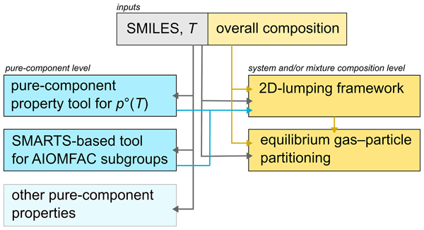
Figure 1 provides a schematic overview of the set of methods used to automate the processing of molecular-level data for gas–particle partitioning calculations and component property characterization. The different pure-component or system-level tools (blue and yellow boxes) will be discussed in separate subsections in the following. The gas-phase chemical mechanisms targeted in our work provide outputs at a selected time in the form of lists of components whose structures are expressed in (or converted to) SMILES format, alongside with the corresponding molecular amounts per unit volume of air, usually provided in units of molec cm⁻³ or mol m⁻³. These lists form the inputs to our multi-model toolchain (Fig. 1). In terms of aerosol applications, one key question concerns how much of the organic mass remains in the gas phase and how much of it contributes to the condensed PM mass concentration under equilibrium conditions. Additional questions concern the hygroscopicity, the potential multi-phase structure of the aerosol material, and related morphology and surface properties. The methods introduced here support answering such questions quantitatively and systematically, even for cases of highly complex chemical mechanism outputs. As indicated in Fig. 1, other temperature-dependent pure-component properties could be determined via existing or new SMILES- and SMARTS-based methods. Such examples include predictions of pure-component surface tension of interest for cloud droplet activation and liquid–liquid interfacial tension (Schmedding et al., 2025; Topping et al., 2007; Schmedding and Zuend, 2025), the solid- and liquid-state densities of organic compounds (Topping et al., 2016; Girolami, 1994), and the glass transition temperature and related pure-component viscosity of interest for molecular diffusion and aerosol mixing timescale modelling (Galeazzo and Shiraiwa, 2022; Armeli et al., 2023; DeRieux et al., 2018).

Figure 1 Schematic overview of the procedures for automatically handling detailed molecular-level data of the numerous components of an organic gas–aerosol system. Component inputs include SMILES for molecular structure, temperature T, and the system's overall (gas plus particle) composition in terms of mass or molar species concentrations. At the pure-component level (blue boxes), SMARTS libraries are employed for estimating pure-component vapour pressure at T and AIOMFAC (functional) subgroup characteristics of each molecule. At the system and/or mixture composition level (yellow boxes), 2D product lumping and surrogate selection is performed based on the volatility, polarity and mass concentrations of the system's organic compounds. Thermodynamic equilibrium partitioning computations are then performed using the selected surrogate system.

As mentioned in Sect. 1.2, the SMILES format is a plain-text notation for describing a component's chemical structure in great detail. SMILES data can be processed by many existing chemical informatics tools. In this work, we make use of the tools based on the Open Babel project, the related Python bindings (via pybel) and/or the application processing interface (API) from the Indigo cheminformatics library (toolkit version 1.7.0) (Pavlov et al., 2011). These third-party libraries can be imported into Python programs. They offer a straightforward means to processing SMILES input, including molecule completeness verification, conversion of generic SMILES into unique SMILES, and the application of customized SMARTS pattern matching. Of note, the Indigo cheminformatics library, even when accessed via its Python library, is running performance-critical computations using an efficient, compiled version of the Open Babel code and Indigo features written in the C++ language.

2.1 Tools for pure-component property predictions

2.1.1 SMILES to AIOMFAC subgroups (S2AS) tool

The SMILES to AIOMFAC subgroups (S2AS) tool is a new, automated algorithm written in Python. It is designed to identify and classify functional groups comprising organic aerosol components in the input format required by the AIOMFAC model. Details of AIOMFAC's representation of molecular structures by a so-called subgroup notation are provided elsewhere (Zuend et al., 2008, 2011); see also examples at https://aiomfac.lab.mcgill.ca/about.html (last access: 25 May 2026). Briefly, the notation of aromatic and aliphatic organic compounds in AIOMFAC is based on that of UNIFAC; e.g. a molecule like ferulic acid (SMILES code: COc1cc(ccc1O)/C=C/C(=O)O), is comprised of the following AIOMFAC subgroups: 1 × (CH=CH), 3 × (ACH), 2 × (AC), 1 × (ACOH), 1 × (CH₃O), 1 × (COOH), where AC denotes aromatic carbon (lower-case c in SMILES). Unlike in SMILES notation, the subgroup input format for AIOMFAC explicitly states the hydrogen atoms, yet the subgroup notation does not contain information about how the subgroups are connected to each other (because AIOMFAC does not require that information). Previously, AIOMFAC subgroup assignments for organic molecules had to be determined either manually (for small sets of structures) or using limited tool-specific pattern matching (e.g., the UManSysProp facility; Topping et al., 2016). Our S2AS tool automates this process for arbitrary molecules. It can process tens of thousands of compounds in a consistent way, whereas manual assignment would be prohibitively laborious and prone to errors or inconsistencies.

We note that the existing list of subgroups in AIOMFAC (about 60 subgroups supported for organic compounds plus special subgroups for inorganics) has limitations when it comes to representing rather exotic, highly functionalized compounds, which may not allow for a perfect mapping by the S2AS tool. Consequently, we implemented a mechanism for detecting and handling exceptions, in most cases by introduction of additional SMARTS patterns to cover these cases. Encountering an exception typically means either that not all atoms can be uniquely associated with only one AIOMFAC subgroup, that a functionality needs to be approximated by an imperfect combination of existing subgroups, e.g. in the case of secondary ozonide functionalities, or that after parsing all existing SMARTS patterns, one or several unmatched atoms remain. Treating such exceptions by an algorithm allows for a consistent, user-independent approximation of the suboptimal mapping. Furthermore, encountered exception cases can be flagged to indicate the potential need for an additional SMARTS pattern to recognize a special case and/or to motivate future improvements by introducing new subgroups into AIOMFAC. To this end, based on our tests with tens of thousands of compounds generated by GECKO-A or MCM (see Sect. 3), unhandled exception cases are a rare occurrence.

The S2AS program carries out the following key steps: (i) parsing of each SMILES string from an input list to determine whether the SMILES input is valid and whether the component falls into the special category of being a pure alcohol or polyol according to the definition used by AIOMFAC; (ii) rendering of molecules for structure visualization as portable network graphics (.png) or scalable vector graphics (.svg) files (this step is optional); (iii) matching substructures to related AIOMFAC subgroups by iterating over a list of SMARTS as outlined in the flowchart of Fig. 2. During step (i), a character string filter is also applied to remove chirality information from input SMILES, which is unnecessary for AIOMFAC subgroups, and to replace radical atoms in a SMILES string by the corresponding non-radical atom (e.g., [O.] by O). The latter is done since AIOMFAC does not support radicals. The pure-component properties and thermodynamic mixing behaviour of such a compound is then approximated by that of a similar non-radical molecule.

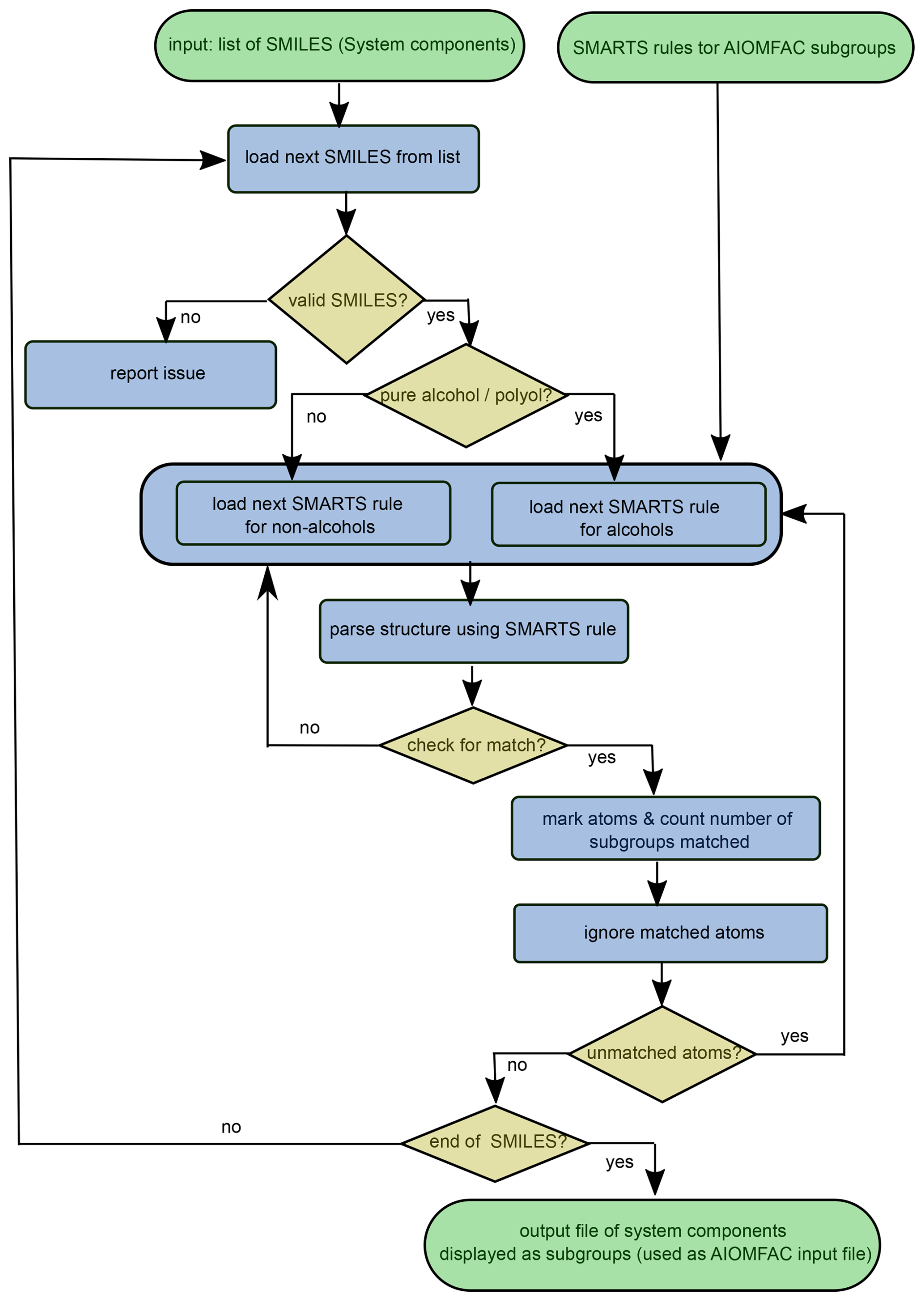
Figure 2 Flowchart illustrating the substructure pattern matching algorithm incorporated in the S2AS tool. SMARTS rules corresponding to all available AIOMFAC functional groups (subgroups) have been formulated in a priority-ordered list; see Table 1.

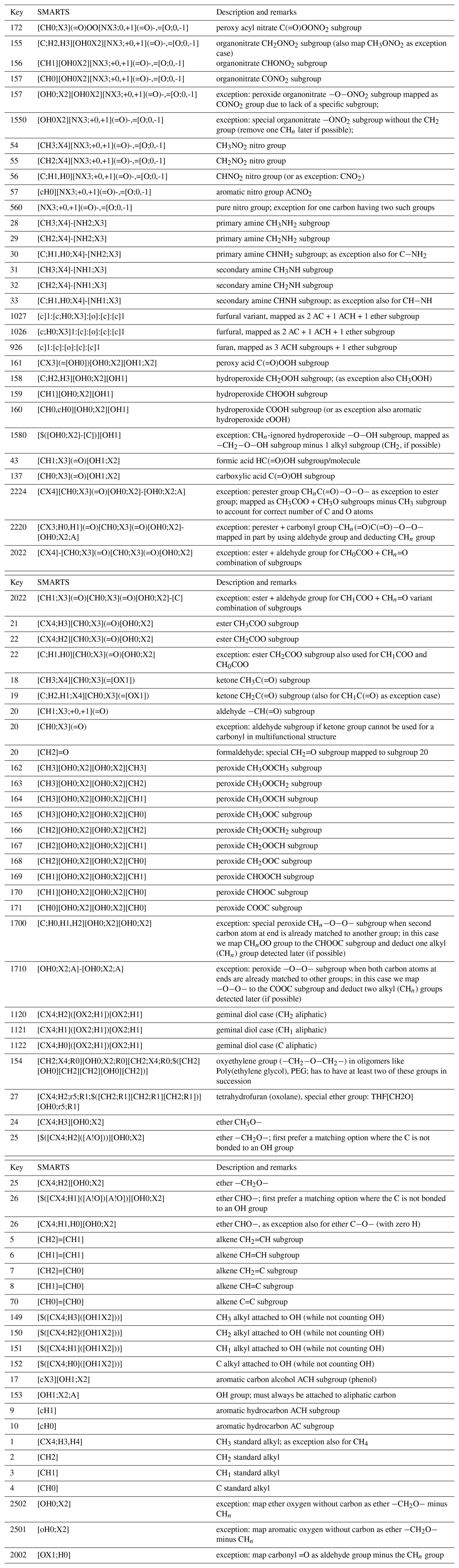
Our implemented SMARTS pattern matching process follows a hierarchical, priority-based querying approach, with relatively large subgroups, such as peroxy acyl nitrate (SMARTS: [CH0;X3](=O)OO[NX3;0,+1](=O)-,=[O;0,-1]), assigned one of the highest matching priorities, while the SMARTS pattern for a single aliphatic carbon bonded to two non-hydrogen atoms and two hydrogens (SMARTS: [CH2]), is among the last patterns applied. The query list and order of SMARTS patterns is provided in Table 1. The company Daylight Chemical Information Systems, Inc., provides manuals, examples and tutorials for understanding and customizing the SMARTS and SMILES languages on their website (https://www.daylight.com, last access: 16 June 2025).

Figures 3 and 4 provide examples of the individual mappings of AIOMFAC subgroups by SMARTS. Alkyl groups, having the lowest matching priority, are matched after all other groups. Pure aliphatic alcohols and polyols are initially detected as such and treated in a separate code branch based on a distinct list of SMARTS, as demonstrated in the example of Fig. 4. Based on the polyol-specific subgroups and nomenclature introduced into a variant of UNIFAC by (Marcolli and Peter, 2005), which is also supported in AIOMFAC, the alcohols and polyols make use of a set of special alkyl subgroups for added specificity and better accuracy of AIOMFAC water uptake and liquid–liquid equilibrium predictions for this class of compounds. A key strength of the S2AS tool is its ability to systematically and efficiently account for the special alkyl groups in a wide variety of straight-chain, branched and cyclical aliphatic alcohols/polyols. For these compounds, the algorithm in S2AS follows a three-step procedure. In step (1) we determine and count the CH_n (n=0, 1, 2, 3) directly bonded to OH groups as well as the associated OH groups, which are separate subgroups. In step (2), we match all alkyl groups belonging to hydrophobic tails by first marking alkyl chains that terminate in $-{\mathrm{CH}}_n-{\mathrm{CH}}_{\mathrm{3}}$ (where n=0, 1, 2) as tails and then iteratively following along those alkyl chains one CH_n group at a time. An alkyl group is part of a hydrophobic tail if, and only if, it connects to at least one other alkyl group known to be part of a hydrophobic tail, while not being bonded to an OH group (those were already determined in step 1). In step (3) all thus far unassigned alkyl groups are detected and classified as being of “alkyl within alcohols” CH_n (n=0, 1, 2, 3) subgroup type.

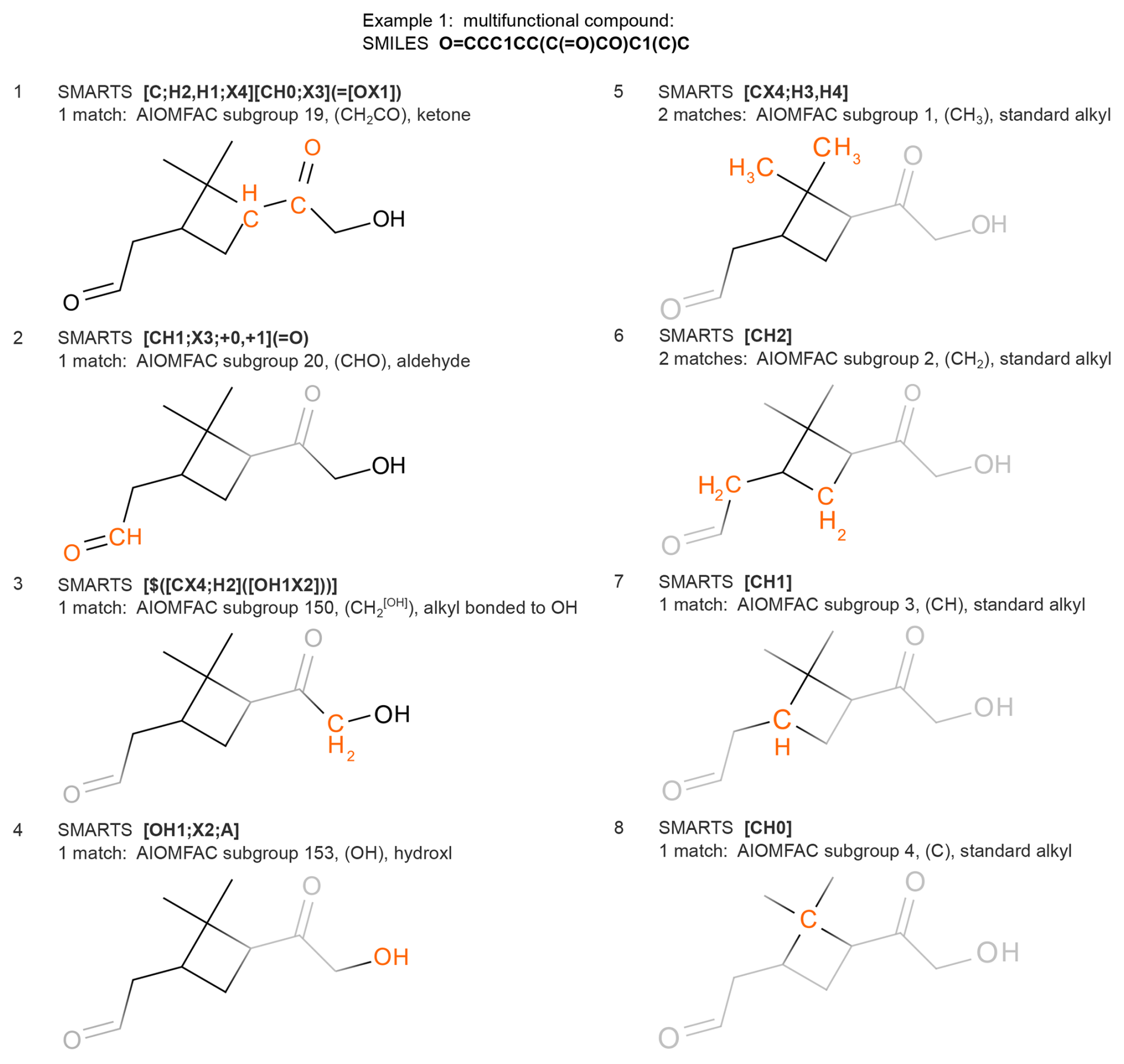
Figure 3 Example of AIOMFAC subgroup determination. Sequences 1–8 show the selection of SMARTS patterns for which at least one match was found, while the structure is probed sequentially by SMARTS from the list (ordered from high to low priority; see Table 1). Atoms matched by a stated SMARTS pattern are highlighted in orange, e.g. the ketone group in panel 1, and subsequently ignored. Light grey colouring denotes ignored atoms/bonds at a certain SMARTS parsing stage.

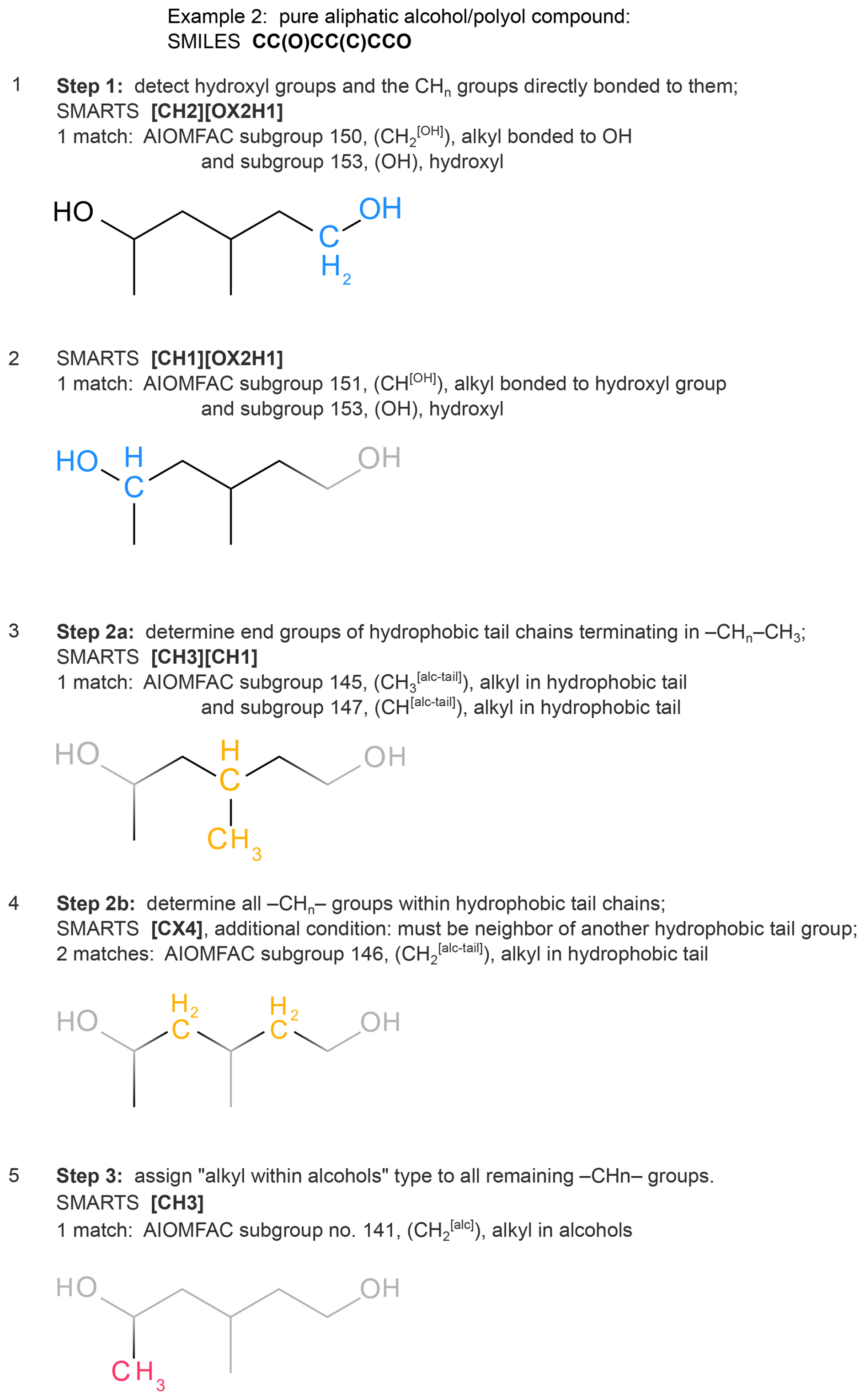
Figure 4 Example of the distinct AIOMFAC subgroup pattern matching applied to pure aliphatic alcohols or polyols, following the distinction of several alkyl group types introduced by Marcolli and Peter (2005). The figure illustrates our three-step algorithm to correctly identify alkyl groups in structures qualifying as pure aliphatic alcohols/polyols. Highlighted SMARTS matches follow the colour scheme of Marcolli and Peter (2005).

In general, the implementation of a hierarchical order and processing of the list of SMARTS is highly advantageous. It allows one to write the SMARTS codes for subgroups of lower priority in a far simpler notation than when each SMARTS code were required to work correctly regardless of the order of execution. For example, if [CH2] were applied as one of the first SMARTS pattern tested, it would likely result in several unwanted matches, such as matching the CH₂ atoms associated with a ketone subgroup (e.g., CH₂CO in AIOMFAC notation); subsequently, the $>\mathrm{C}=\mathrm{O}$ of the remaining atoms of the ketone group would not be detected as being part of a full ketone subgroup (clearly a mistake). To avoid this, the SMARTS pattern for only detecting intended CH₂ groups would need to be much more complicated, such that it would avoid matching atoms that could be matched as part of a bigger substructure. When a SMARTS match is found for the molecule under consideration, the corresponding matched atoms are marked and excluded from further parsing if unmatched atoms remain in the component; the Indigo toolkit provides “ignore atom” and “highlight atom” functions that conveniently aid in avoiding any unwanted double-matching of atoms. A numerical counter corresponding to the key of the matched SMARTS rule and associated subgroup is incremented for each successful pattern match and added to the subgroup-array representation of the compound for later S2AS output. After all atoms have been matched or when the end of the list of SMARTS is reached, a check is performed to determine whether any unmatched atoms remain in a given molecule, potentially indicating an exception case (very rare). After, the next molecule from the SMILES list is processed. Once all SMILES have been processed, the S2AS program outputs a text file in the format of AIOMFAC-web input files (see examples at https://aiomfac.lab.mcgill.ca/about.html, last access: 25 May 2026).

To validate the S2AS tool and associated SMARTS patterns, we used a comprehensive data set of aerosol-relevant organic compounds, including those produced by MCM v3.3.1 simulations for monoterpenes and alkanes, an excerpt is shown in Fig. 5. These tests serve as proof of concept of the tool's ability to extract and convert detailed molecular information from a diverse range of compounds commonly encountered in atmospheric chemistry simulations.

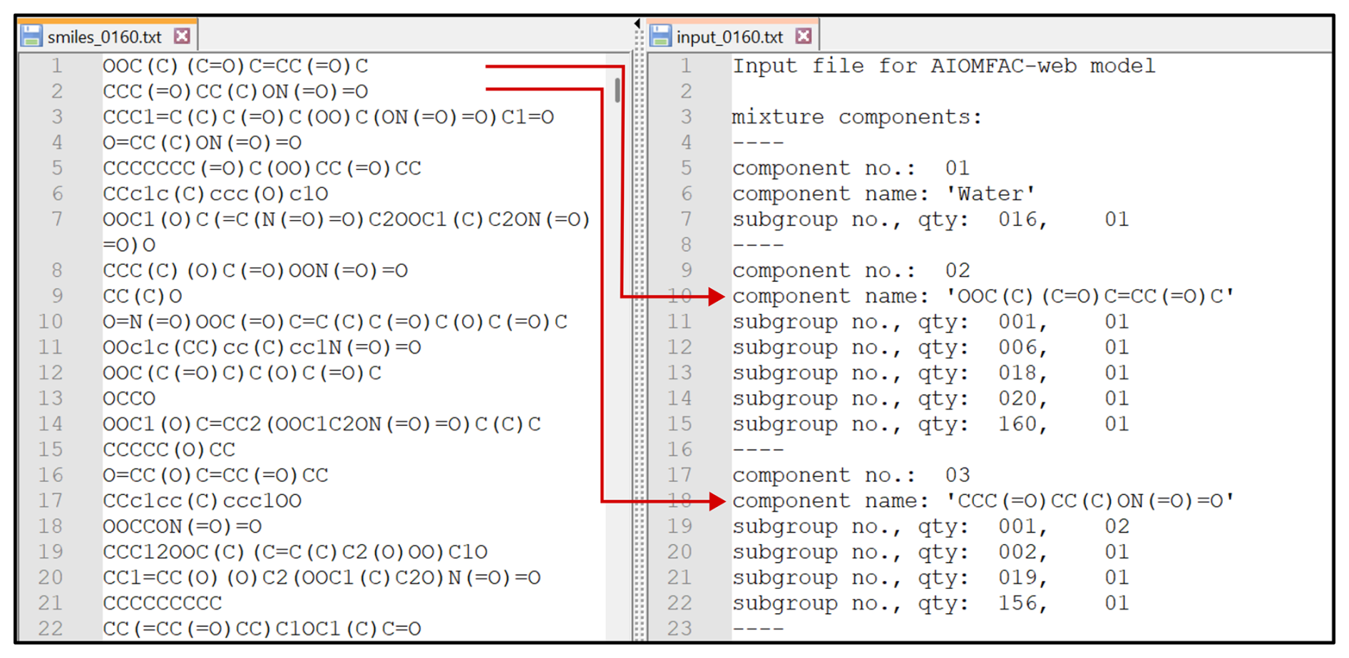
Figure 5 A sample subset of input SMILES strings on the left hand side and their corresponding output functional subgroups generated by the S2AS tool on the right hand side. The generated text file can serve as input file for the AIOMFAC model alongside with mixture composition information.

2.1.2 Pure-component vapour pressure estimation

The UManSysProp project developed by Topping et al. (2016) is an open-source facility that employs cheminformatics tools for molecular and mixture property predictions. This facility allows users to input molecular information in the SMILES format, from which the relevant information for aerosol property calculations are extracted (Topping et al., 2016). This tool utilizes the Open Babel and pybel cheminformatics libraries for the parsing of molecules using tool-specific SMARTS pattern matching, similar to the AIOMFAC-specific S2AS procedure described in Sect. 2.1.1. Of most relevance for this study, the pure-component, liquid-state saturation vapour pressure tool, available as part of the UManSysProp facility, provides several methods for estimating temperature-dependent vapour pressures. It uses method-specific SMARTS pattern matching to calculate the pure-component vapour pressures using predictive models, including the Estimation of VApour Pressure of ORganics, Accounting for Temperature, Intramolecular, and Non-additivity effects (EVAPORATION) model (Compernolle et al., 2011), the model by Nannoolal et al. (2008), hereafter called Nanoolal method, and the SIMPOL method (Pankow and Asher, 2008). The source code for the original and subsequent releases of UManSysProp is available from an online repository (see code and data availability). We note that UManSysProp also includes a few tools for aerosol mixture predictions, including a version of the AIOMFAC model and related SMARTS patterns for generating AIOMFAC input data. However, the list of SMARTS patterns for AIOMFAC in UManSysProp differs in several ways from the more extensive SMARTS list and related S2AS program introduced in this study. Specifically, Topping et al. (2016) do not follow the same SMARTS priority order, use a different, less comprehensive approach for handling matching exceptions, and the way pure alcohol compounds are detected and mapped may differ as well for more complex polyols. Hence, SMARTS codes from their study are not directly transferrable for use in the S2AS tool.

Several studies have compared liquid-state pure-component vapour pressure prediction methods suitable for SOA systems alongside with critical evaluations of existing experimental data for the particularly relevant semi-volatile and low-volatility compounds. It has been shown that, when applicable, the EVAPORATION method and the Nanoolal method are among the best performing options in those volatility ranges of particular importance for the gas–particle partitioning of SOA (e.g., Barley and McFiggans, 2010; O'Meara et al., 2014; Bilde et al., 2015). The Nanoolal method is more versatile in terms of the variety of functional groups and chemical elements covered, while the EVAPORATION method is constrained to compounds containing the elements C, H, O, N. However, these are also the main elements supported in AIOMFAC and we opted to use the EVAPORATION method as our first choice for the lumping framework and the gas–particle partitioning calculations.

The parameterization of the temperature-dependence of pure-component vapour pressures used in our work is identical to the two-parameter relation introduced for the EVAPORATION model (Compernolle et al., 2011):

$$\begin{array}{}\text{(1)}& {\log }_{\mathrm{10}}\left[{\displaystyle \frac{p_j^{\circ }}{p^{\text{ref}}}}\right]=A_j+{\displaystyle \frac{B_j}{T^{\mathit{\kappa }}}}.\end{array}$$

Here, $p_j^{\circ }$ denotes the pure-component, liquid-state (saturation) vapour pressure of component j in units of atmospheres (atm) and p^ref=1 atm is the unit reference pressure. T is the temperature (K), and A_j and B_j are two component-specific parameters. A common value of κ=1.5 was adopted based on optimization tests by Compernolle et al. (2011). It was shown to be appropriate for estimating vapour pressure of hydrocarbons with or without heteroatoms across a wide temperature range. The A_j and B_j values are directly predicted by the EVAPORATION model. Alternatively, they can be determined by running any pure-component vapour pressure prediction method at two sufficiently distinct temperatures (typically ΔT>30 K), including the temperature interval of interest, followed by solving the system of two linear equations for A_j and B_j. The use of Eq. (1) enables the flexibility of $p_j^{\circ }$ estimation at any reasonable temperature for the given set of input molecules, serving as a key input to the gas–particle partitioning model. Computing the A_j, B_j parameters for all organic aerosol system components once eliminates the need for calling the EVAPORATION model repeatedly when the temperature changes, thus improving computational efficiency.

This approach streamlines the application of distinct SMILES-based tools for (any) pure-component properties and enhances the flexibility of the gas–particle partitioning model in terms of its readiness for computations being carried out over a range of temperatures. In summary, the UManSysProp pure-component property models (written in Python) are run for a given list of SMILES characterizing a system. The A_j and B_j parameters and corresponding SMILES of all organic system components are then written to a text file for read-access by other tools. In particular, the list of parameters is read by the Fortran code of the AIOMFAC equilibrium model, which makes subsequent use of Eq. (1) to obtain the $p_j^{\circ }$ at a temperature of interest. The pure-component vapour pressure files are also used in the 2D lumping framework described next.

Table 1 Priority-ordered SMARTS query list for the parsing of non-polyol aliphatic and aromatic organic component SMILES and associated matching to the corresponding AIOMFAC subgroups. The key value indicates the corresponding AIOMFAC subgroup identifier a pattern will be mapped to – or, in exception cases (values >300), an index for exception handling by the S2AS program.

2.2 2D lumping framework

We implemented a new variant of a two-dimensional product lumping framework with the aim to (1) categorize and visualize a representation of all oxidation and fragmentation products from an organic aerosol system at a given point in time and (2) to enable an objective, yet adjustable, selection of surrogate species for a reduced-complexity representation of the system. We constructed a 2D space for mapping the entire aerosol component system using the logarithm of the pure-component vapour pressure, ${\log }_{\mathrm{10}}[p_j^{\circ }/(\mathrm{1}\mathrm{Pa}\left)\right]$, as the volatility dimension (x axis). This choice is similar to that of 1D VBS models and several 2D VBS variants, which typically either use the pure-component saturation vapour concentration ($C_j^{\circ }$ in units of µg m⁻³) or the effective saturation concentration ($C_j^{\star }$ in units of µg m⁻³) on a logarithmic scale as volatility dimension (Donahue et al., 2006, 2011). Assuming the ideal gas law to apply, pure-component vapour pressures and pure-component saturation concentrations can be inter-converted via (Zuend and Seinfeld, 2012)

$$\begin{array}{}\text{(2)}& C_j^{\circ }=p_j^{\circ }{\displaystyle \frac{M_j}{RT}}\cdot {\mathrm{10}}^{\mathrm{9}}\left[\mathrm{\mu }\mathrm{g}{\mathrm{kg}}^{-\mathrm{1}}\right].\end{array}$$

Here, M_j is the molar mass (kg mol⁻¹) and R the universal gas constant ($\mathrm{J}{\mathrm{mol}}^{-\mathrm{1}}{\mathrm{K}}^{-\mathrm{1}}$). Several metrics exist for representations of an organic molecule's effective polarity, including the elemental O:C ratio and the average oxidation state of carbon, denoted by ${\stackrel{\mathrm{‾}}{\text{OS}}}_{\mathrm{C}}$ (Kroll et al., 2011). In the case of atmospheric organics consisting of the elements carbon, hydrogen, nitrogen and oxygen, typically the approximation ${\stackrel{\mathrm{‾}}{\text{OS}}}_{\mathrm{C}}\approx \mathrm{2}\cdot \left(\mathrm{O}:\mathrm{C}\right)\mathrm{-}\mathrm{H}:\mathrm{C}-\mathrm{5}\cdot \left(\mathrm{N}:\mathrm{C}\right)$ applies (Kroll et al., 2011). Our framework offers those metrics as optional choices, yet our preferred choice for the polarity axis (y axis) of the lumping framework is to use a metric based on the logarithm of an activity coefficient ratio (ACR) (as detailed in Sect. 2.2.1 and defined by Eq. 5).

In the context of gas–particle partitioning in aerosol systems as a main application of the 2D lumping framework, one way to guide appropriate choices for the two dimensions of the framework is to consider the main factors governing absorptive gas–particle partitioning (Pankow, 2003). Zuend et al. (2010) derived that for equilibrium gas–particle partitioning involving an ideal gas phase and a single (liquid) condensed phase, the following relationship must hold for $K_j^{\text{PM},\left(n\right)}$, the equilibrium partitioning coefficient on a molar basis:

$$\begin{array}{}\text{(3)}& K_j^{\text{PM},\left(n\right)}={\displaystyle \frac{x_j^{\text{PM}}}{p_j}}RT={\displaystyle \frac{\mathrm{1}}{{\mathit{\gamma }}_j^{\left(x\right)}{p}_j^{\circ }}}RT.\end{array}$$

Here, $x_j^{\text{PM}}$ is the mole fraction of component j in the liquid particulate matter (PM) phase, p_j is the partial pressure in the gas phase (ideal gas assumption), and ${\mathit{\gamma }}_j^{\left(x\right)}$ is the activity coefficient in the liquid phase (superscript (x) denotes mole-fraction-based quantities). While $p_j^{\circ }$ indicates the importance of a component's saturation vapour pressure, ${\mathit{\gamma }}_j^{\left(x\right)}$ indicates the influence of nonideal mixing in the liquid phase. The degree of nonideal mixing depends both on the molecular properties of j as well as its interactions with all other molecules in solution. In this context, a polar organic compound present in an aqueous phase will exhibit a lower activity coefficient than a nonpolar compound. Hence, activity coefficients offer a way to express a component's affinity for less or more polar liquid media. This supports the choice of proxies for polarity as the second dimension of our 2D framework. We note that for aerosol systems undergoing liquid–liquid phase separation (LLPS), Eq. (3) holds when appropriately modified, such as by introducing a phase-abundance-weighted effective activity coefficient (Zhang et al., 2024).

2.2.1 Activity coefficient ratio as polarity metric

The idea of using an activity coefficient ratio (ACR) as a polarity metric is inspired by liquid–liquid equilibrium (LLE) thermodynamics. In a macroscopic LLE state, the chemical potential of a component present in both coexisting phases must be identical. Consequently, the way a component j partitions between two liquid phases, α and β, can be described using an equilibrium partitioning constant $K_j^{\left(x\right)}$ (Zuend and Seinfeld, 2013; Topping and Bane, 2022):

$$\begin{array}{}\text{(4)}& K_j^{\left(x\right)}={\displaystyle \frac{x_j^{\mathit{\alpha }}}{x_j^{\mathit{\beta }}}}\stackrel{\text{LLE}}{=}{\displaystyle \frac{{\mathit{\gamma }}_j^{\mathit{\beta },\left(x\right)}}{{\mathit{\gamma }}_j^{\mathit{\alpha },\left(x\right)}}}.\end{array}$$

Here, $x_j^{\mathit{\alpha }}$ and $x_j^{\mathit{\beta }}$ are mole fractions in phases α and β; ${\mathit{\gamma }}_j^{\mathit{\alpha },\left(x\right)}$ and ${\mathit{\gamma }}_j^{\mathit{\beta },\left(x\right)}$ are the activity coefficients in those phases under LLE conditions. Equation (4) indicates that knowledge of the ${\mathit{\gamma }}_j^{\mathit{\beta },\left(x\right)}/{\mathit{\gamma }}_j^{\mathit{\alpha },\left(x\right)}$ ratio provides an accurate representation of the thermodynamic phase preference of organic components by quantifying the relative enrichment or depletion of a component via the equivalent mole fraction ratio, with a value greater than 1 indicating enrichment in phase α. Since activity coefficients depend on a phase's mixture composition established by all components, the values are sensitive to various forms of molecular interactions (e.g., dipole–dipole, dispersion) and reflect the chemical affinity for a phase. That is, activity coefficients are influenced by molecular structure properties, such as whether an oxygen-bearing functional group is more polar (e.g., hydroxyl, carboxyl) or less polar (e.g., ether, ester) and how it interacts with other organic and inorganic components present. Thus, the ACR encompasses more detailed functional group characteristics than simpler metrics like the O:C ratio.

In this work, the ACR of a component j is based on a prediction of the component's activity coefficient when present as a dilute solute in a weakly polar organic reference solvent, here we use 1,2-hexanediol, relative to that of being a dilute solute in a strongly polar reference solvent, here water. This metric is therefore similar to the well-established octanol–water partitioning coefficient (e.g., Kamlet et al., 1988; Wienke et al., 1998), but our choice of organic reference solvent differs. We elected to use a slightly more polar organic than octanol, with 1,2-hexanediol serving as a more typical representation of an organic-rich phase medium in aerosols.

While inspired by the LLE isoactivity condition (Eq. 4), the procedure of obtaining our ACR metric differs from that of solving a ternary solute–solvent-1–solvent-2 LLE problem. This is because in the ternary LLE system the present solvents may be partially miscible, while we choose to compute the activity coefficients of each component independently based on evaluating two binary solute–solvent mixtures. Using binary systems as a gauge is computationally simpler and substantially faster. Specifically, our polarity metric ACR is defined by the following dimensionless quantity:

$$\begin{array}{}\text{(5)}& {\log }_{\mathrm{10}}\left[{\displaystyle \frac{{\mathit{\gamma }}_{j,\text{hex}}^{\left(x\right)}}{{\mathit{\gamma }}_{j,\mathrm{w}}^{\left(x\right)}}}\right].\end{array}$$

Here, ${\mathit{\gamma }}_{j,\text{hex}}^{\left(x\right)}$ is the (predicted) mole-fraction-based activity coefficient of solute j in a binary mixture with the solvent 1,2-hexanediol, in which the mass fraction of j is w_j=0.01 (therefore, w_hex=0.99). Analogously, for ${\mathit{\gamma }}_{j,\mathrm{w}}^{\left(x\right)}$, except for the solvent being water. These activity coefficients are typically evaluated at a reference temperature of 298.15 K. Given this definition, one can think of these two separate activity coefficients, as well as their ratio, as pure-component properties. In principle, those values would only need to be computed once for each component (each SMILES code) and could then be saved and retrieved from a look-up table.

The selection of the two reference solvents provides a robust basis for characterizing the behaviour of organic components across a wide range of polarities spanning several orders of magnitude (see Sect. 3). In our framework, the AIOMFAC model is employed to compute activity coefficients for Eq. (5). Since AIOMFAC is run only for binary, single-phase systems, the calculations are fast; they are comparable or faster than the pure-component vapour pressure predictions with UManSysProp. Of note, for a system consisting of tens of thousands of organic components, computing activity coefficients of all species simultaneously using the related multicomponent mixtures (containing as many components) with AIOMFAC, is prohibitively slow due to the many functional groups present, all the possible group–group and molecule–molecule interactions that need to be summed over and the associated computer memory requirements. In contrast, computing the ACR values based on the binary solute–solvent mixtures for all those components is fast and small in memory footprint.

2.2.2 Methods for surrogate selection

We implemented four distinct methods to analyze organic aerosol data in the 2D lumping framework and to objectively select a set of surrogate components. These methods are designed to reduce the complexity of the gas–aerosol system while preserving important physicochemical aspects, such as the conservation of total mass concentration and the consideration of the system's diversity in terms of volatility and polarity ranges. The four methods are: (a) the grid cell midpoint method, (b) the grid cell medoid method, (c) the grid cell mass-weighted medoid method, and (d) the k-means-based medoids method. The latter is a grid-independent 2D clustering method.

The 2D space is subdivided into a number of grid cells (or clusters) based on the targeted reduction in system complexity. This division is accomplished by specifying the number of rows and columns, followed by identification of the component coordinates that set the upper and lower coordinate limits within the range that should be gridded (see use of a volatility threshold below). The grid resolution is adjustable, but typical choices range from 2×1 to 20×10 in terms of setting the number of grid subdivisions and associated n_x×m_y grid cells.

A crucial aspect of our methodology is the primary focus of the gridded domain on the compound volatility ranges of interest for substantial partitioning of organics to the particle phase. These volatility ranges includes semi-volatile (SVOC), low-volatility (LVOC) and extremely low-volatility (ELVOC) organic compounds, while intermediate volatility (IVOC) and volatile organic compounds (VOC) are too volatile under typical tropospheric aerosol mass loading conditions (Donahue et al., 2012; Zuend and Seinfeld, 2012). As such, an adjustable high-volatility vapour pressure threshold (p_high) is introduced, typically set to ${\log }_{\mathrm{10}}(p_{\text{high}}/[\mathrm{1}\mathrm{Pa}\left]\right)>-\mathrm{1}$. Regardless of the polarity range, all compounds with $p_j^{\circ }>p_{\text{high}}$ are identified and lumped into a single high-volatility surrogate component using the mass-weighted medoid method defined below. Examples for this are shown in Sect. 3, e.g., Figs. 7 and 8. Since the p_high threshold value is an input parameter, this special VOC lumping step can also be avoided entirely by setting a very high threshold value. Similarly, a low-volatility threshold and related lumping of LVOC and ELVOC compounds into a single (or a few), quasi-nonvolatile surrogate could be introduced to focus the majority of surrogates on representing the SVOC range at comparably higher resolution. However, in this work we have not included a low-volatility threshold since we are interested in a diverse surrogate-based representation of all PM-relevant volatility ranges to better resolve potential trends in polarity with decreasing volatility accross the SVOC, LVOC, and ELVOC ranges.

Our lumping process adheres to the principle of mass conservation for the entire system. This is achieved by aggregating the mass concentrations of components within each grid cell or cluster into the selected surrogate component. This approach differs from methods that choose to conserve the number of carbon atoms during lumping. The surrogate component selection process for each of the four methods is visually depicted in Fig. 6. The shown examples illustrate how one surrogate component is chosen within a single grid cell (or cluster in case of k-means).

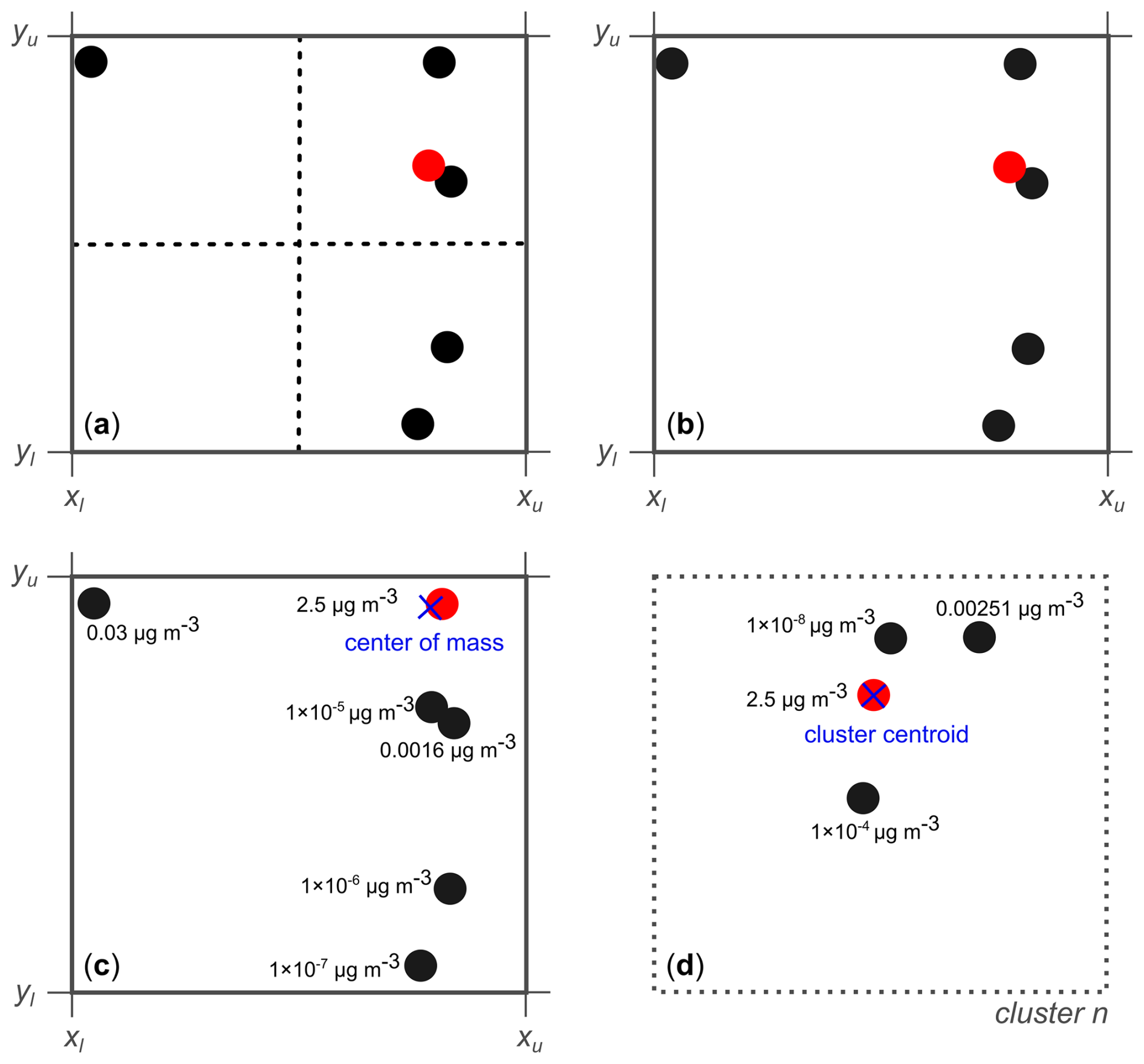
Figure 6 Illustration of the four introduced methods for selecting a single surrogate component (marked in red) within a specific grid cell or cluster of the 2D space. x_l and x_u indicate the lower and upper x axis values of the grid cell; analogously for y_l and y_u. (a) The midpoint method selects a surrogate based on the component closest to the geometric centre of the grid cell, denoted by the dotted lines. (b) The medoid method selects the component with the smallest cumulative Euclidean distance from all other components. (c) The mass-weighted medoid method prioritizes components with higher mass concentrations. It determines the most representative surrogate as the one closest to the centre of mass established by the components in the cell. (d) The k-means-based medoid method is independent of a grid. It iteratively assigns components to clusters, then identifies a cluster's optimal surrogate as the nonzero-mass component closest to the cluster centre (indicated by the blue × symbol). Individual clusters are not confined to predetermined grid cells (in d denoted by dotted outline); here, the four points are assumed to form a specific cluster n.

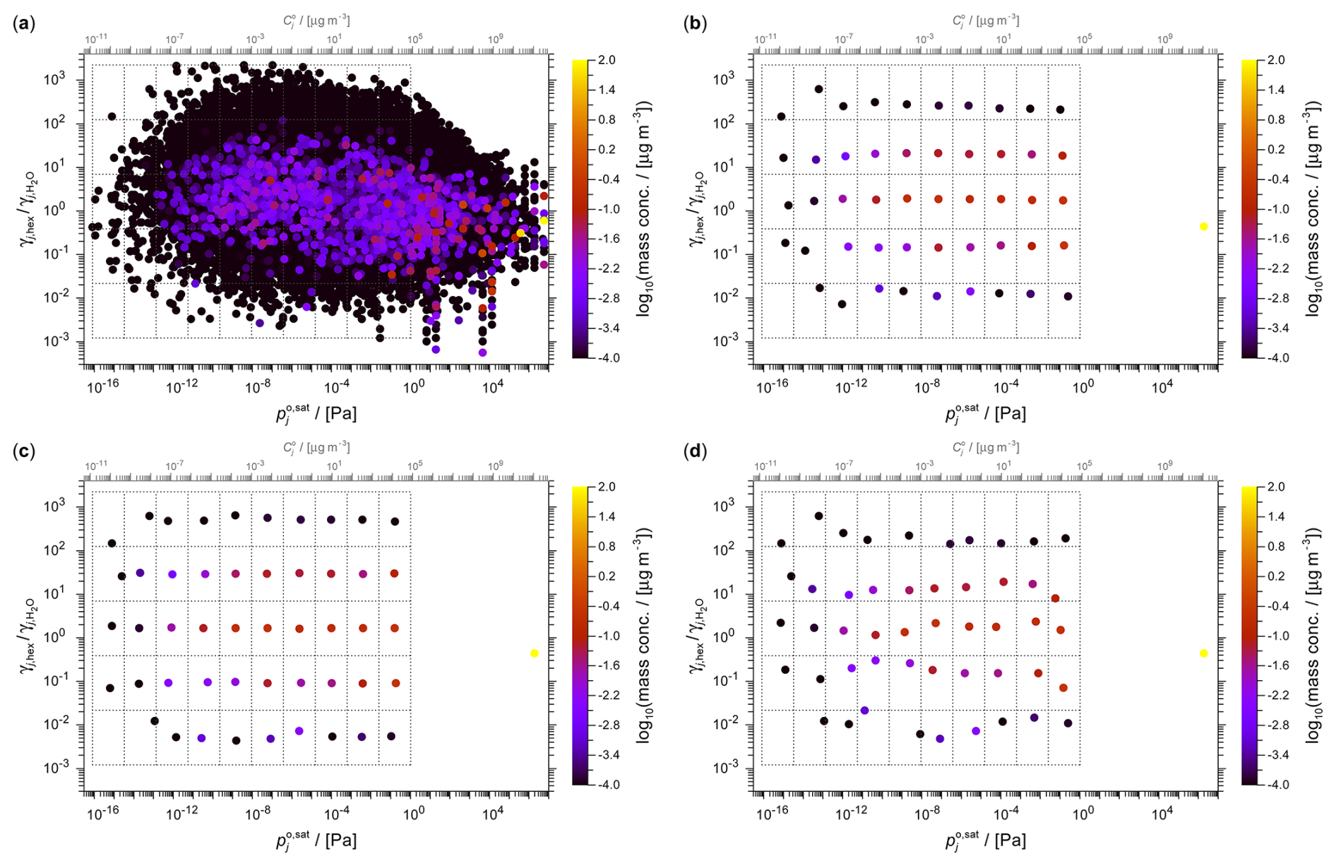
Figure 7 The toluene SOA system shown in the 2D space of activity coefficient ratio versus saturation vapour pressure at 298 K. (a) The full set of ∼68 000 components derived from a simulation based on the GECKO-A mechanism with an overlaid 10×5 grid (dotted) which is used by the different selection methods to determine grid cell surrogates. (b–d) Surrogates selected by (b) the medoid method, (c) the midpoint method and (d) the weighted medoid method. The top horizontal axis indicates the approximate pure-component saturation vapour concentration corresponding to the vapour pressure axis (see details in Sect. S2).

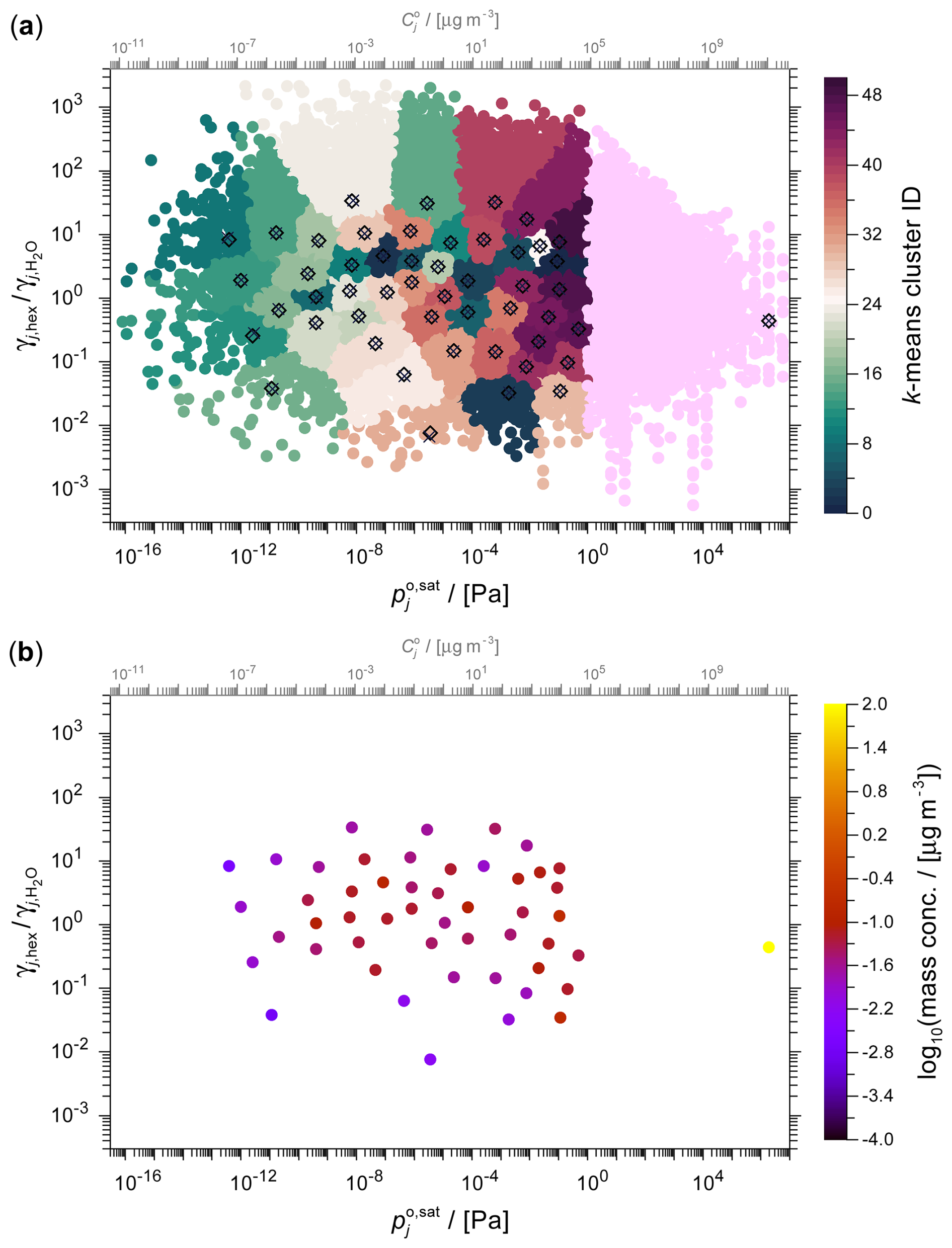
Figure 8 2D space representations of the toluene-derived SOA system at 298 K using the k-means clustering and surrogate selection method. (a) 49 clusters plus 1 high-volatility cluster (pink data points) are shown with individual cluster members identified by the same colour. The cluster centres are denoted by × and the corresponding selected cluster surrogates by the ⋄ symbols. (b) The lumped mass concentrations of the surrogate components selected by the mass-weighted k-means method (see Table S5 for related surrogate data).

2.2.3 Grid cell midpoint method

The midpoint method operates on the simple principle that the component closest to a grid cell's midpoint coordinates should be a reasonable choice representing all other components within the same cell. This method involves determining the normalized distance of each grid cell component's location to the grid cell midpoint. The squared Euclidean distance, $D_{\text{mid},i}^{\mathrm{2}}$, of each component i within a grid cell is calculated by

$$\begin{array}{}\text{(6)}& D_{\text{mid},i}^{\mathrm{2}}={\left[{\displaystyle \frac{x_{\text{mid}}-x_i}{x_{\text{range}}}}\cdot \mathit{\chi }\right]}^{\mathrm{2}}+{\left[{\displaystyle \frac{y_{\text{mid}}-y_i}{y_{\text{range}}}}\right]}^{\mathrm{2}}.\end{array}$$

Here, x_mid and y_mid denote the midpoint coordinates of the grid cell, x_i and y_i are the coordinates of component i, and x_range and y_range denote the magnitudes of the x and y axes ranges of the 2D space over which the lumping grid was placed. They normalize the distances expressed along the two axes. The x-to-y aspect ratio χ is introduced to scale the normalized length scales of the grid space. That is, χ is the (prescribed) multiplying factor of the normalized, dimensionless value range along the x axis that is regarded as equivalent to the normalized, dimensionless range along the y axis. To express the importance of volatility in gas–particle partitioning, we elected to set a 2:1 aspect ratio as the default choice. If the number of grid lines along the x-dimension is already set as twice that of the y-dimension (e.g., 8 by 4), then χ will account for this (χ=1 in that case). In this study, the x-coordinate refers to the logarithm of the pure-component vapour pressure (${\log }_{\mathrm{10}}(p_i^{\circ }/[\mathrm{1}\mathrm{Pa}\left]\right)$), while the y-coordinate corresponds to one of the proxies for polarity (ACR, O:C ratio, ${\stackrel{\mathrm{‾}}{\text{OS}}}_{\mathrm{C}}$). The value ranges of the components along the x and y coordinates may differ substantially, possibly by several orders of magnitude. Therefore, we chose to normalize and scale the magnitudes of the x and y axes ranges relative to each other, as shown by Eq. (6). The x_range ($=|x_{max}-x_{min}|$) is determined by the maximum and minimum x-coordinates from the set of all system components that contribute nonzero mass concentration and belong to the regular lumping space, i.e., those not lumped to the single high-volatility surrogate compound. The y_range is determined analogously. Finally, within each grid cell containing at least one component, the component of minimum $D_{\text{mid}}^{\mathrm{2}}$ is selected as surrogate and the mass concentrations of all other grid cell members are lumped (additively) into the surrogate. Except for the method-specific expressions for computing a component's distance metric within a grid cell, the variable definitions and steps outlined for this method also apply to the other methods described in the following sub-sections.

The grid cell midpoint method is straightforward to understand and implement. It has the advantage of providing unbiased coverage of the 2D space by ensuring that surrogate components are nearly evenly distributed across the grid domain. The approach demonstrates scalability, as it can be easily applied to systems with a large number of components, making it suitable for complex mixture analyses. Additionally, the method offers computational efficiency since the calculation of midpoints and distances is relatively fast, even for large datasets. However, this method may not always select the most representative component, especially when a low-resolution grid is applied in which the few cells may exhibit unevenly distributed components (e.g., all components clustered around the lower left corner of a cell). This method is visualized in Fig. 6a.

2.2.4 Grid cell medoid method

The grid cell medoid method operates by selecting the medoid component of each grid cell as the surrogate. The medoid member is the component in closest cumulative proximity to all other components of the same cell. Therefore, the main step involves calculating the cumulative squared Euclidean distance of each component from all other components of the grid cell, as follows:

$$\begin{array}{}\text{(7)}& \mathrm{\Sigma }{D}_{\text{med},i}^{\mathrm{2}}=\sum _{j=\mathrm{1}}^m{\left[{\displaystyle \frac{x_j-x_i}{x_{\text{range}}}}\cdot \mathit{\chi }\right]}^{\mathrm{2}}+{\left[{\displaystyle \frac{y_j-y_i}{y_{\text{range}}}}\right]}^{\mathrm{2}}.\end{array}$$

Here, index j covers the $\mathrm{1},\mathrm{\dots },m$ components of the grid cell, with other variables as defined for Eq. (6).

The medoid method offers potential advantages over the midpoint method. First, it may provide better representation by selecting a surrogate that is located close to most other components, which is especially of importance in the case of a grid space with only a few large cells filled with geometrically uneven component distribution. Second, the medoid method demonstrates robustness to outliers, being less influenced by extreme values or uneven clustering of points within a cell compared to the midpoint. In comparison to the midpoint method, the medoid method is computationally more costly, especially for cells that contain a large number of components. However, in practice this is rarely a concern. Figure 6b illustrates the grid cell medoid method.

2.2.5 Grid cell mass-weighted medoid method

The mass-weighted medoid method prioritizes surrogate selection based on a combination of a component's importance, as measured by its mass concentration, and the cumulative distance from other components of a grid cell, as in the unweighted medoid method. Using such a mass-weighted approach is particularly useful in the case of systems consisting of many components, yet with the majority of the mass contributed by a small minority of molecules. The mass-weighting ensures that the important components are more likely to be selected as surrogates, so that their particular molecular properties are then also more appropriately considered in subsequent equilibrium partitioning computations. The core of this method lies in the calculation of the squared distance between a component and the coordinates of the centre of mass of the cell, $D_{\text{wmed},i}^{\mathrm{2}}$, as follows:

$$\begin{array}{}\text{(8)}& D_{\text{wmed},i}^{\mathrm{2}}={\left[{\displaystyle \frac{x_{\text{mc}}-x_i}{x_{\text{range}}}}\cdot \mathit{\chi }\right]}^{\mathrm{2}}+{\left[{\displaystyle \frac{y_{\text{mc}}-y_i}{y_{\text{range}}}}\right]}^{\mathrm{2}},\end{array}$$

with

$$\begin{array}{}\text{(9)}& \begin{array}{rl}& x_{\text{mc}}=\sum _{j=\mathrm{1}}^m{w}_j\cdot x_j,y_{\text{mc}}=\sum _{j=\mathrm{1}}^m{w}_j\cdot y_j,\mathrm{\text{and}}\\ & w_i={\displaystyle \frac{C_i}{{\sum }_{j=\mathrm{1}}^m{C}_j}}.\end{array}\end{array}$$

Here, x_mc and y_mc are the coordinates of the centre of mass of the grid cell under consideration. These coordinates are determined by computing the mass-weighted average coordinates of the $j=\mathrm{1},\mathrm{\dots },m$ grid cell components, as shown by Eq. (9), only requiring information about the cell's components of nonzero mass concentration. w_j and C_j represent a component's grid-cell mass fraction and mass concentration, respectively. Components of large mass concentration relative to others in a grid cell have the effect of “pulling” the centre of mass toward their location, thereby benefiting from a smaller $D_{\text{wmed},i}^{\mathrm{2}}$. Among the grid cell components of nonzero mass concentration, the component of minimum $D_{\text{wmed},i}^{\mathrm{2}}$ value is identified as the surrogate. Components of zero mass concentration are excluded from the calculation and from being selected as surrogate.

This method strongly favours the selected surrogate components to be from the subset of most abundant species in the gas–aerosol system. The mass-weighted medoid method offers several advantages. The method provides improved representation of dominant components. The resulting lumped system is likely to reflect bulk aerosol properties more accurately, especially when only a low-resolution grid is applied. To aid in understanding the interplay between mass concentration and spatial distribution in the surrogate selection process, Fig. 6c exemplifies how the component of highest mass concentration, which is also closest to the centre of mass within the grid cell, is selected as the surrogate component.

2.2.6 k-means-based clustering method

The mass-weighted, k-means-based medoid clustering method, for brevity hereafter referred to as the k-means method, is employed to generate a predefined number of centroids (k clusters) in the 2D space. The clustering process is implemented using a variant of the weighted k-means clustering algorithm; specifically, subroutine kmeans_w_01, from the Fortran 90 implementation provided by Burkardt (2008). The Fortran code is based on the theory, algorithm and existing code from the works by Sparks (1973) and Hartigan and Wong (1979). This algorithm iteratively reassigns points (here chemical components) to clusters, minimizing the total energy of the system. Refer to Sparks (1973) and Hartigan and Wong (1979) for a detailed description of the k-means method and its variants.

In our approach for surrogate selection with the k-means method, we combine the mass-weighted clustering with a final, distance-based surrogate component selection process. Figure 6d visualizes an example cluster's surrogate selection. Specifically, k-means returns the coordinates of a predefined number of cluster centres, which usually do not coincide with any actual component's coordinates. Among each cluster's population, we then select the component of nonzero mass concentration that is located closest to the cluster centre coordinates as the cluster's surrogate. Similar to the mass-weighted medoid approach, the distance of each cluster component to the centre is determined by the squared Euclidean distance based on normalized coordinates. In outcome, this is therefore akin to (but algorithmically not identical with) the method of k-medoids clustering.

By selecting surrogate species that are typically centrally located within their clusters and of significant mass concentration, this approach ensures that the set of surrogate components represents the overall physicochemical characteristics of the system well. This approach is particularly valuable in atmospheric chemistry, where reducing the complexity of chemical mechanisms while retaining properties of the most abundant components is crucial, since mass or number concentration of components is a critical factor in understanding subsequent partitioning or chemical reaction behaviour.

In our implementation, the clustering process begins by setting the desired number of k clusters. The initial cluster centre coordinates are then set based on the grid cell midpoints (since in our code the grid-based methods are run prior to running k-means). For comparison with the grid-based methods, we typically chose the cluster numbers as being equal to the number of populated grid cells. However, the k-means clustering method can also be run independently from the gridded approaches. If a higher number of clusters is set as target than the number of populated grid cells, additional initial cluster centre coordinates are generated using pseudo-random coordinates within the scaled 2D space. This initialization step ensures a broad distribution of initial cluster centres across the normalized 2D space. Components associated with the special high-volatility surrogate are filtered out, since they are marked as being part of a special cluster; these are not considered during the k-means clustering.

An innovation of the weighted k-means variant is the incorporation of, in our case, mass-concentration-based weighting during the algorithm's assignment of components to clusters. When k-means computes each cluster's “energy” and iteratively assigns components to a certain cluster, the weights are factored in. As discussed in Sect. 3, actual example cases indicate that the mass concentrations of components may range over several orders of magnitude. Therefore, the weighting aids in prioritizing components with relatively high mass concentrations as potential cluster surrogates, ensuring that the clustering process is not solely based on spatial proximity. The algorithm considers the entire dataset simultaneously and can effectively handle cases in which data points are not uniformly distributed in a 2D space. While we favour weighted k-means clustering, if desired, one can assign each component the same weight, thereby returning to the non-weighted k-means method.

Overall, the k-means method offers several advantages. The method can identify natural groupings in the data, independent of the arbitrary limits of an imposed grid, potentially leading to more meaningful, unbiased surrogate selection. However, this method is computationally the most costly of the four outlined in this study. Users can adjust the targeted number of k-means clusters to strike a balance between model simplicity and resolution of the original data. We note that the computational cost of this method is relatively insensitive to the number of clusters targeted.

3 Results and discussion

The primary goals of this study were to develop efficient and practical tools for calculating pure-component properties, activity coefficients and the gas–particle partitioning for complex systems containing a large number of organic species. To this end, we implemented and evaluated a 2D lumping framework to reduce system complexity while maintaining an adjustable level of accuracy. Additionally, we sought to compare the effectiveness of different lumping methods. These objectives were pursued to advance our understanding of organic species behaviour and improve computational efficiency in geoscientific modelling. The S2AS pure-component property prediction tool was implemented in Python. The 2D lumping framework was implemented in modern Fortran. The generated computer programs are a main product of this work. Related code and data are provided via code repositories and version-specific archives (see Sect. Code and data availability).

3.1 Example systems: α-pinene and toluene oxidation products

To demonstrate the application of the new chain of software tools, we introduce two example systems showcasing a multitude of chemical components and related properties derived from simulations of (1) an α-pinene ozonolysis system simulated using the MCM (v3.3.1) model and (2) a toluene photo-oxidation system simulated based on a near-explicit GECKO-A mechanism of its gas phase chemistry. The input parameters used for these simulations are listed in Tables S1 and S2 in the Supplement. The system component structures were either directly output or subsequently converted to the SMILES format and the component concentrations retrieved from a selected output time of the simulations. For the examples shown, the output data at the final time of a respective mechanism simulation was used.

The GECKO-A toluene photolysis system comprises an extensive array of ∼68 000 distinct organic components. Figure 7 provides a visual representation of the obtained system of oxidation and fragmentation products in the 2D polarity versus volatility space. The complete set of components is shown in Fig. 7a (ordered by mass concentration to show the most abundant components on top), while panels (b)–(d) show the application of a 10×5 volatility × polarity (here using ACR) grid to select surrogate components by the three grid-based methods. Figure 8 shows the corresponding data clustered by the k-means method and the pertaining selection of surrogate components. The comparison of the full system and the various surrogate representations demonstrate visually the framework's ability to simplify complex chemical systems. Despite the massive reduction in the number of species, our lumping framework successfully preserves key physicochemical characteristics of the system of relevance for SOA formation predictions.

The 2D representation of the α-pinene-derived components is shown in Fig. 9, with panel (a) showing the full set of MCM-derived system components. Panels (b)–(d) of Fig. 9 show the surrogate selections based on a 10×5 grid. Since several grid cells are empty in this example, only 36 surrogates are determined at the chosen grid resolution. Figure 10 demonstrates the application of the k-means method to this system when using ACR as the polarity axis. Table S6 summarizes the surrogate properties from this k-means clustering example.

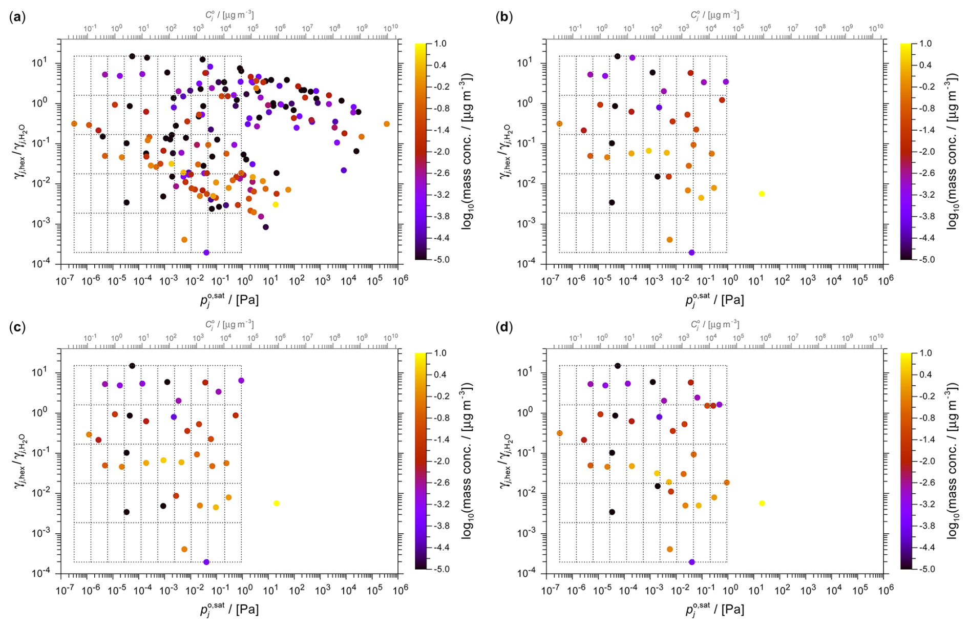
Figure 9 The α-pinene SOA system components shown in the 2D space of activity coefficient ratio versus vapour pressure at 298 K. (a) The full MCM-derived 174 components with an overlaid 10×5 grid (dotted) that is used by the different selection methods to determine grid cell surrogates. (b–d) Surrogates selected by (b) the medoid method, (c) the midpoint method and (d) the weighted medoid method.

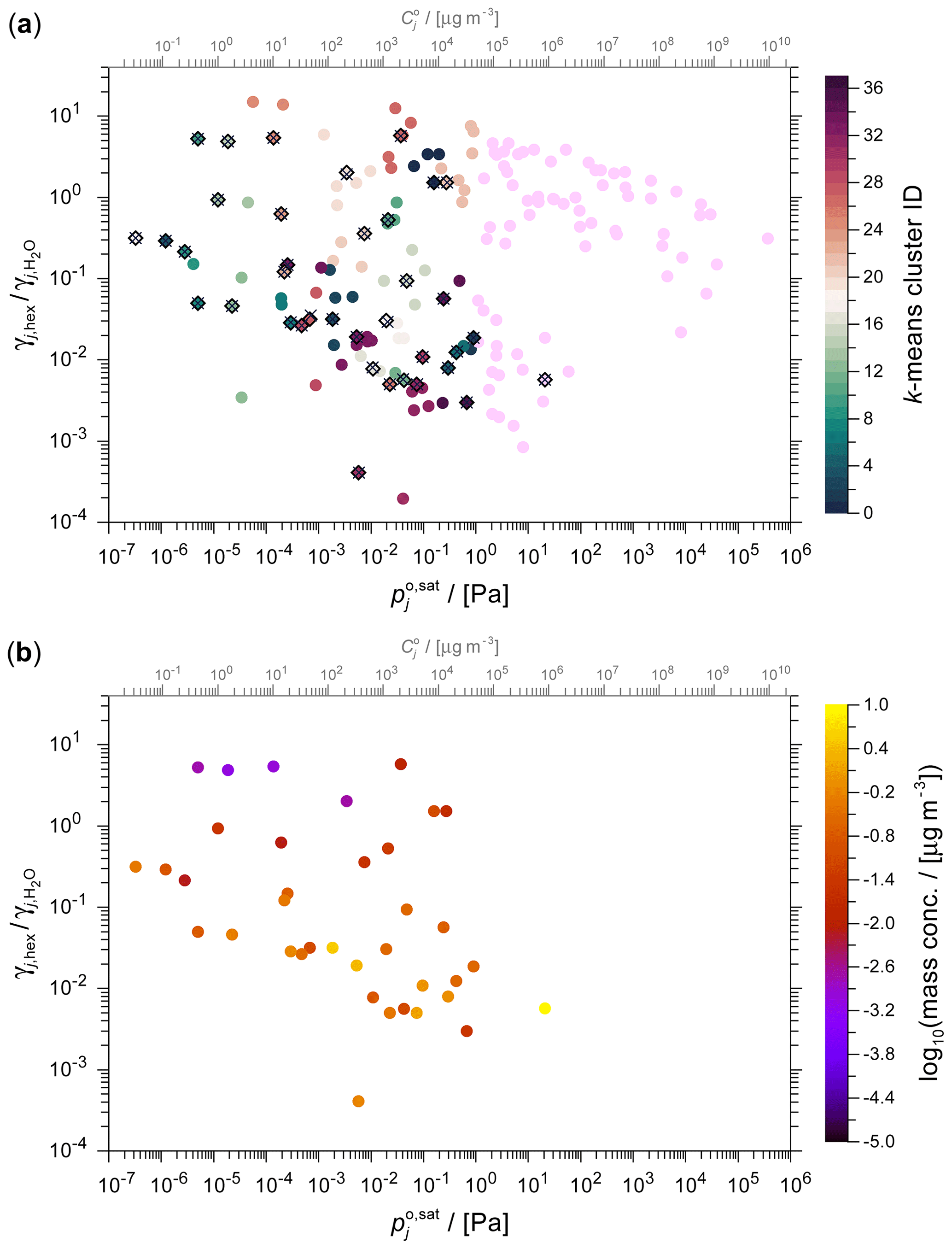
Figure 10 2D space representations of the α-pinene SOA system at 298 K using the k-means clustering and surrogate selection method. (a) 36 clusters are shown with individual cluster members identified by the same colour. The cluster centres are denoted by × and the corresponding selected cluster surrogates by the ⋄ symbols. Data points coloured pink are members of the special high-volatility cluster. (b) The lumped mass concentrations of the surrogate components selected by k-means (see Table S6 for related surrogate data).

3.2 Performance of automated property prediction tools

3.2.1 Functional group identification (S2AS tool)

The S2AS tool demonstrated high accuracy in identifying AIOMFAC functional groups for the α-pinene and toluene oxidation products. The 174 α-pinene-derived products were mapped to AIOMFAC subgroups without needing any exception treatments, while an average of 0.5 exceptions (special SMARTS mappings) per molecule were encountered in case of the ∼68 000 toluene-derived products. The latter exhibited a higher level of nitrogen-containing functional groups, some of which were responsible for most of the exception cases triggered. Given the systematic handling of exception cases, the S2AS tool was successful in mapping all carbon, oxygen and nitrogen atoms to relevant subgroups. This is particularly noteworthy given the structural complexity of many of the oxidation products, which often contain multiple functional groups, branched functionalized chains and ring structures. The S2AS tool is also more reliable than manual classification in cases involving complex molecular structures, for which human experts may occasionally overlook less prominent functional groups or perform inconsistent exception treatments when an imperfect mapping to the available set of AIOMFAC subgroups is present.

The S2AS tool showed high computational efficiency in processing large datasets. It successfully processed the list of 174 α-pinene oxidation product SMILES in less than 0.8 s, and the ∼68 000 SMILES from the toluene system in ∼5 min – a processing rate of ∼13 800 SMILES per minute on a single laptop processor core (1 thread, Intel Core i7-10710U CPU). This automatic classification rate represents a tremendous advance over manually assigning AIOMFAC subgroups for each component, which would be an infeasible task for systems containing thousands of components. The S2AS tool's processing speed scales linearly with dataset size. Further speedup via parallelization on multi-core computers is possible, but such enhancements have not been attempted in the current version of the source code.

3.2.2 Vapour pressure estimation

The UManSysProp pure-component vapour pressure estimation tool demonstrated robust performance across the wide range of molecular structures present in the α-pinene and toluene oxidation systems. It successfully parsed the list of SMILES and predicted the vapour pressures for all molecules. For the examples shown in this study, we used the output from the EVAPORATION method, yet the seven other pure-component vapour pressure prediction methods available from UManSysProp were also completed successfully.

The version of UManSysProp we employed in this work includes a new module we developed to determine a two-parameter temperature dependence parameterization of pure-component vapour pressures using the form of Eq. (1) for each of the vapour pressure methods included (not just EVAPORATION). In a first step, a component's vapour pressure is predicted by each method at seven temperatures equally spaced between 260 and 320 K. In a second step, the two parameters of Eq. (1) are fitted to these data for each method. In the case of EVAPORATION, no fitting is required since one can solve for parameters A_j and B_j using the output from the end points of the temperature range (two equations, two unknowns). If speed is of the essence, the parameter fitting step can also be bypassed for all other methods by solving for the parameters in the same way, usually yielding similar parameter values to those obtained from a more elaborate fit. The single-thread processing of the ∼68 000 toluene-derived product SMILES took 482 s on a Intel Core i7-10710U CPU (one thread) for the vapour pressure data creation plus 83 s for determining the parameters A_j and B_j pertaining to each method when bypassing the parameter fitting step. This amounts to a SMILES processing rate of $\sim \mathrm{120}{\mathrm{s}}^{-\mathrm{1}}$ or ∼7200 SMILES per minute (including the parameter fitting step reduces the rate to ∼1650 SMILES per minute). As in the case of the S2AS tool, further speed-up is possible by introducing parallel processing (with good scaling potential) in the case of extensive lists of SMILES.

Together with the introduced S2AS, these two pure-component property prediction tools enable automated and efficient processing of SMILES data for atmospheric and environmental chemistry applications.

3.3 Evaluation metrics for the 2D lumping framework

To facilitate an evaluation of the 2D lumping framework in terms of impacts of polarity axis choices and grid resolutions, we performed 2D lumping at several grid resolutions, each followed by AIOMFAC-based equilibrium gas–particle partitioning computations to generate aerosol properties of interest for a quantitative comparison. Specifically, we calculated the mean absolute percentage error (MAPE) and mean percentage error (MPE) for the resulting SOA mass concentrations as well as the aerosol hygroscopicity parameter κ. Aerosol mass concentration and hygroscopicity are two (among several) insightful characteristics of the (gas–)aerosol partitioning behavior and water uptake potential. The MAPE and MPE are relative deviation metrics defined as follows:

$$\begin{array}{}\text{(10)}& {\displaystyle }\text{MAPE}={\displaystyle \frac{\mathrm{1}}{n}}\sum _{i=\mathrm{1}}^n\left|{\displaystyle \frac{F_i-A_i}{A_i}}\right|\times \mathrm{100}\mathit{\%},\text{(11)}& {\displaystyle }\text{MPE}={\displaystyle \frac{\mathrm{1}}{n}}\sum _{i=\mathrm{1}}^n\left({\displaystyle \frac{F_i-A_i}{A_i}}\right)\times \mathrm{100}\mathit{\%}.\end{array}$$

Here, A_i represents the actual (observed or reference) value, F_i the predicted value, and n is the number of observations. MAPE is scale-independent, making it useful for comparing overall prediction precision across different datasets (especially datasets free of extreme outliers). MPE measures the average bias in the predictions relative to the reference data. By considering the direction of errors, MPE complements MAPE by highlighting any systematic high or low biases in the model's predictions, which can be crucial for understanding the limitations and potential improvements of each method.

MAPE and MPE were calculated for a selection of grid resolutions (4×2, 6×3, 8×4, 10×5) and polarity axis metrics for both α-pinene-derived SOA and toluene-derived SOA. In order to calculate the evaluation metrics for the toluene SOA system, for which a full-system calculation was not feasible with the AIOMFAC equilibrium partitioning model, the mass-weighted k-means method with the ACR polarity axis and a higher 25×10 grid resolution was used as the reference (benchmark case) for all relative deviation evaluations. A validation check was also carried out using the k-means method for a 40×20 grid resolution (also with ACR as polarity axis) to verify whether the MAPE and MPE values across different (higher) grid resolutions and associated numbers of k-means clusters, were consistent with the reference case. The predicted reference mass concentration at the 25×10 grid resolution (219 surrogates) agrees with that from the 40×20 (612 surrogates) case within a MAPE of 0.1 %, confirming it to be an appropriate reference.

Table 2 compares the relative deviations of different surrogate selection methods for predicting SOA mass concentrations using the selected surrogate species from the α-pinene SOA system. The table lists the MAPE and MPE for the four surrogate selection methods (midpoint, medoid, mass-weighted medoid, mass-weighted k-means) combined with three polarity axis options across different grid resolutions. The corresponding absolute SOA mass concentrations and κ values predicted for this system are listed in Table S3. The weighted k-means method generally performs best, with lowest errors across most grid sizes. Table 3 presents similar MAPE and MPE data but for the predictions of the hygroscopicity parameter κ for the same α-pinene SOA system. Again, the weighted k-means method tends to show the smallest errors overall compared to other surrogate selection approaches. A more detailed discussion of different axis choices and impacts follows in the “Analysis of the polarity axes and surrogate selection methods” part.

Table 2 Comparison of relative deviations in predicted SOA mass concentrations at 298 K for the α-pinene-derived SOA system. The MAPE and MPE values are listed for the four different surrogate selection methods combined with three choices for the polarity axis (y axis) and for several grid/cluster resolutions. The reference values are from the partitioning computation based on the full system (174 organic components). For a comparison of related absolute quantities, see Table S3.

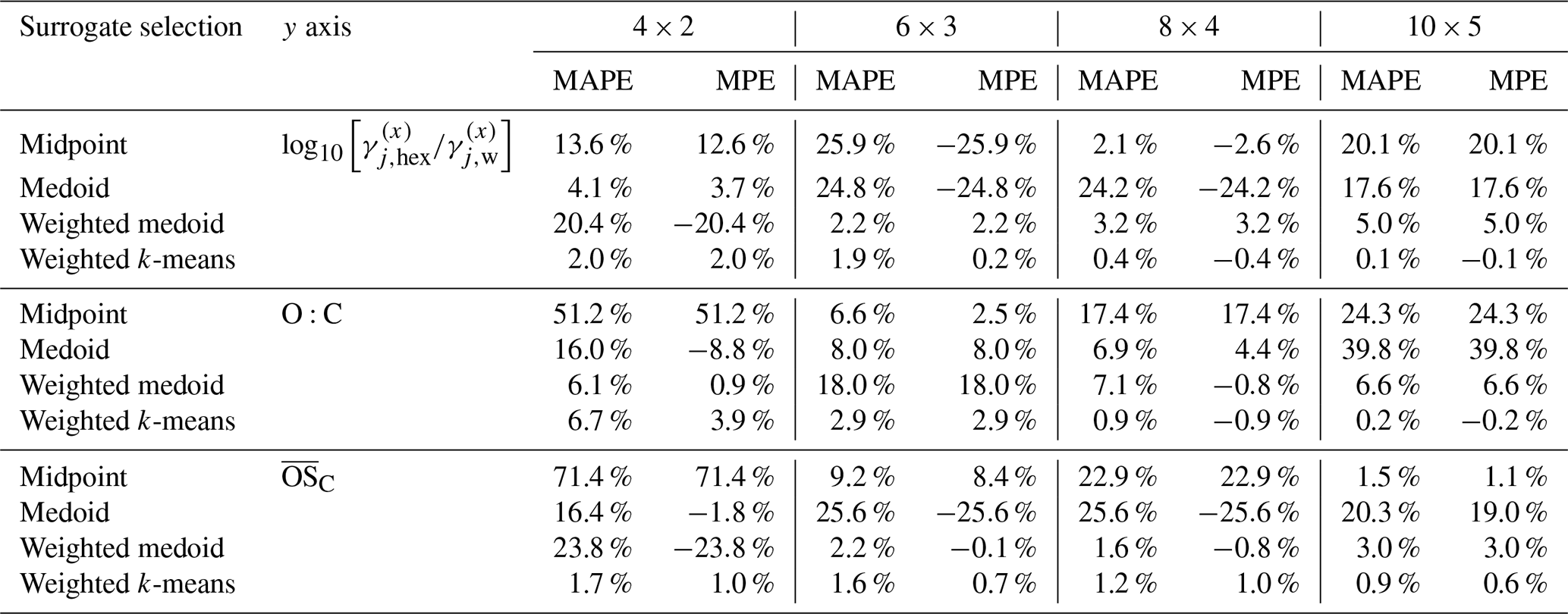
Table 3 Similar to Table 2 but for the MAPE and MPE of the predicted hygroscopicity parameter κ (evaluated at water activities of 85 % and 90 %) relative to the full α-pinene SOA system prediction used as benchmark.

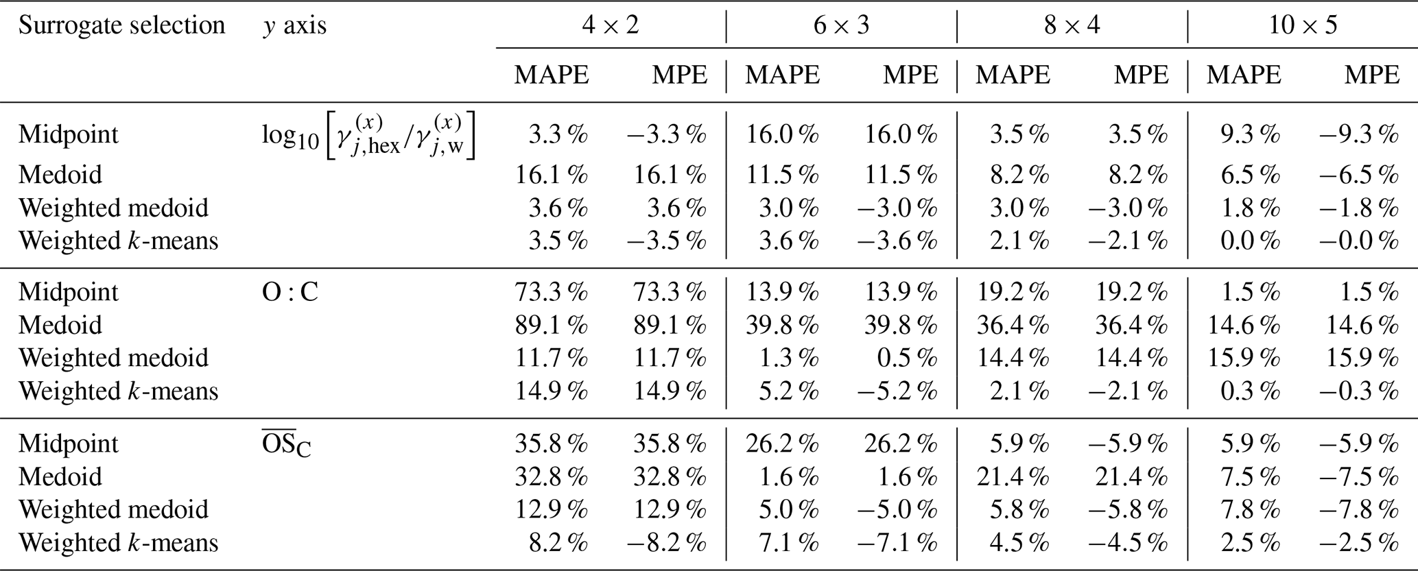
Table 4 provides MAPE and MPE values for SOA predictions from the toluene oxidation system, comparing the same surrogate selection methods and polarity metrics across five grid resolutions. Table 5 shows the corresponding evaluation of the hygroscopicity parameter predictions for the toluene-derived SOA. The corresponding absolute SOA mass concentrations and κ values predicted for this system are listed in Table S4. Deviations from the reference case at lower grid resolutions are generally higher than for SOA mass predictions, but the mass-weighted k-means method still performs relatively well at most resolutions. The larger variability in κ predictions stems in part also from the relatively low absolute values (Table 7). Additionally, the relatively small modelled SOA mass concentrations contribute to the observed metric fluctuations, since minor absolute differences can result in larger relative errors.

Table 4 Comparison of relative deviations in predicted SOA mass concentrations at 298 K for the toluene-derived SOA system. The MAPE and MPE values are listed for the four different surrogate selection methods combined with three choices for the polarity axis and for several grid/cluster resolutions. The computation with the mass-weighted k-means method using the ACR polarity proxy at 25×10 resolution (219 surrogate components) is used as reference for MAPE and MPE calculations. For related absolute quantities, see Table S4.

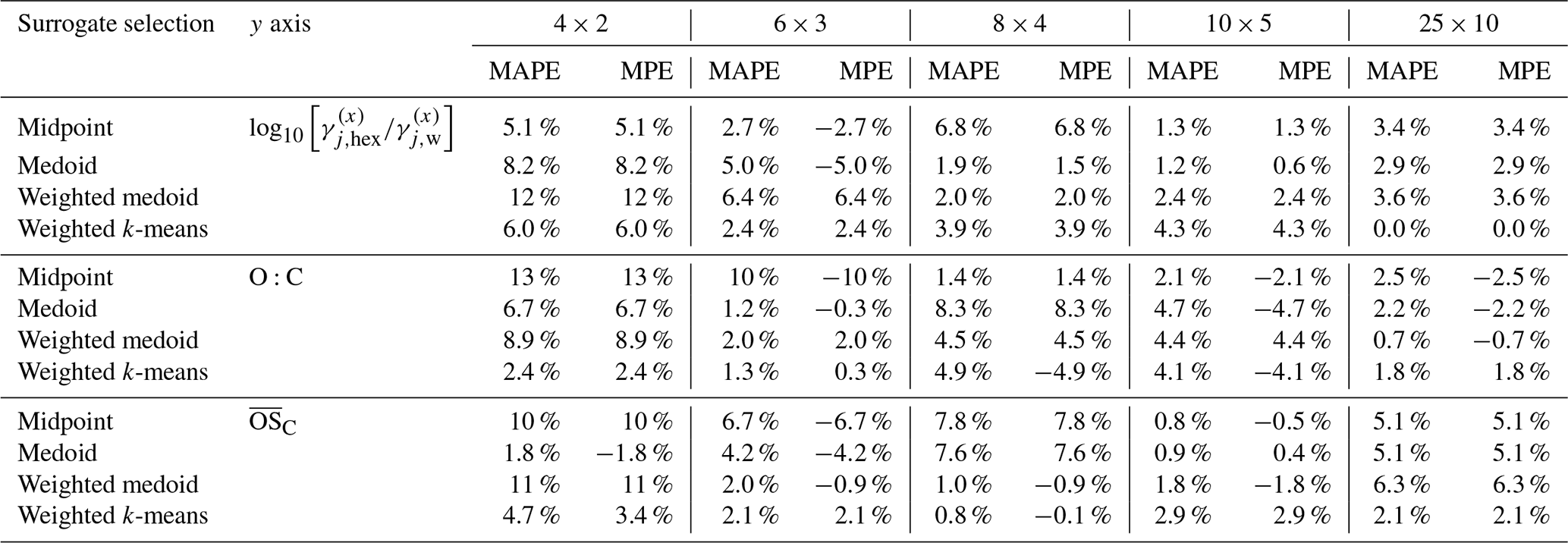
Table 5 Similar to Table 4 but for the MAPE and MPE of the predicted hygroscopicity parameter κ of the predicted toluene-derived SOA (evaluated at water activities of 85 % and 90 %). The mass-concentration-weighted k-means method at 25×10 resolution is used as reference case.

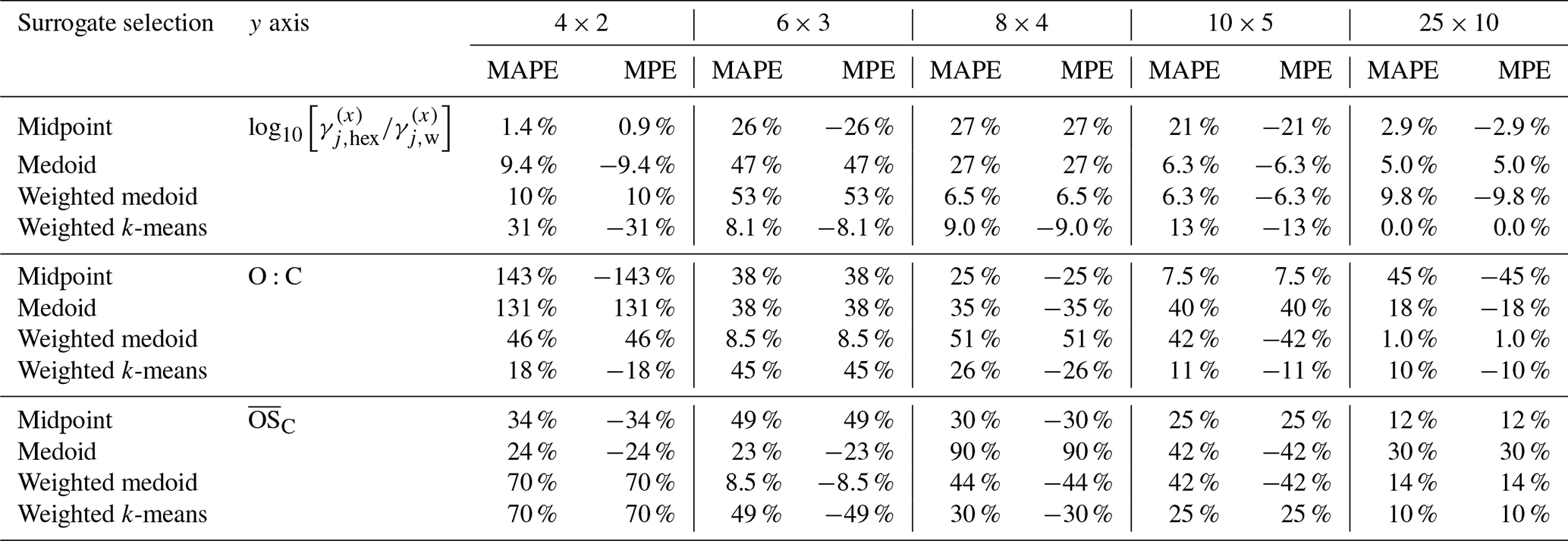
Table 6 compares the predicted aerosol mass concentrations for the toluene and α-pinene SOA systems at different water activities, using the weighted k-means method or, in case of α-pinene SOA, the full system for the model calculations. In both cases, the predicted SOA mass concentrations are relatively low (<2 or <4 µg m⁻³), yet in a realistic range for relatively clean air quality conditions. These absolute SOA mass concentrations may contribute to the observed fluctuations in MAPE and MPE for different resolutions and polarity axis choices, since minor absolute differences can result in larger relative deviations.

Table 6 Comparison of predicted SOA mass concentrations at selected water activities (equilibrium RH) for the toluene and α-pinene SOA systems. For the toluene SOA system, the data are based on ACR as the polarity axis, 25×10 resolution and k-means surrogate selection. The full set of MCM-derived system components is used for the α-pinene SOA case.

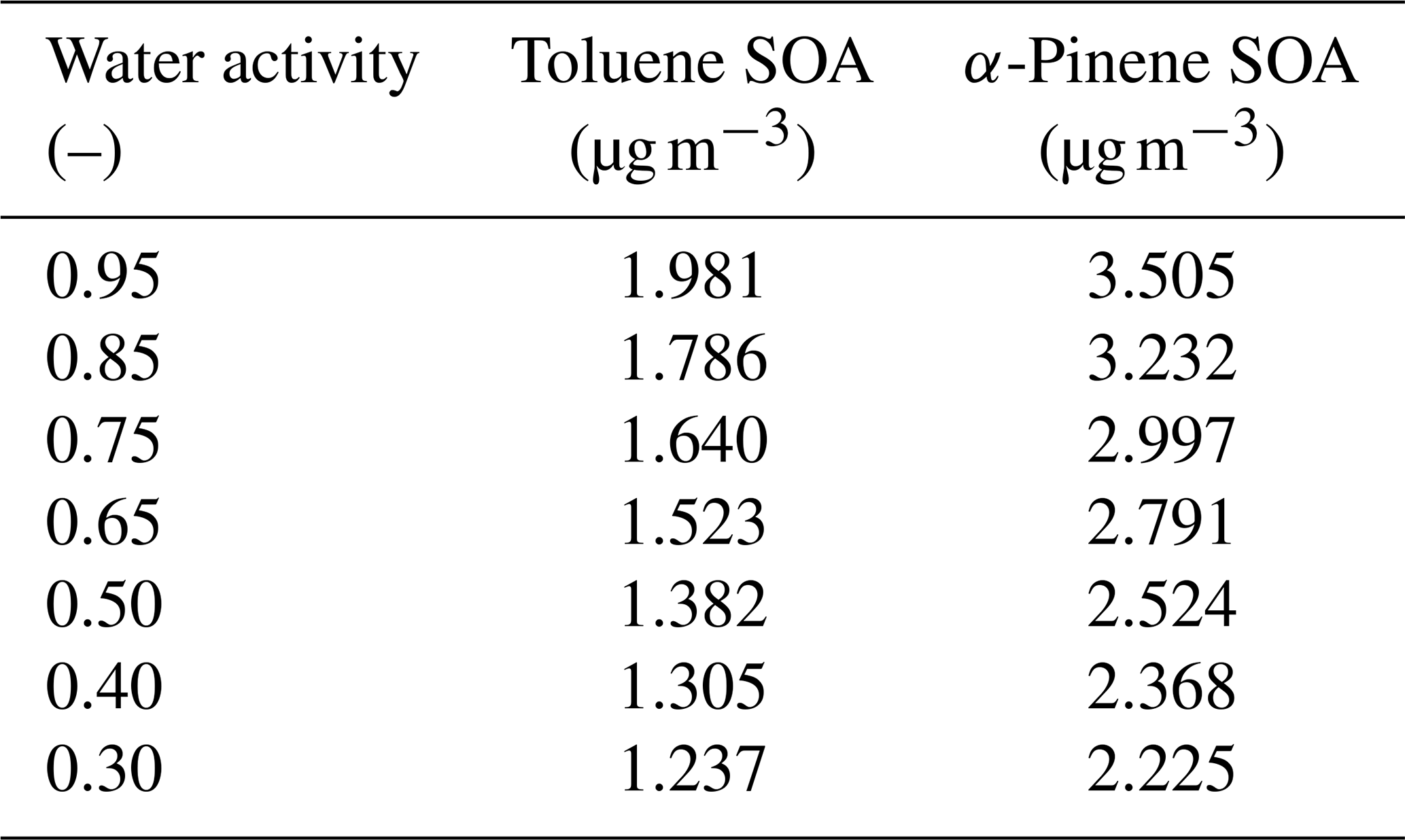
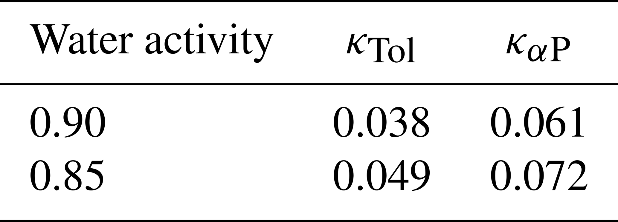
Table 7 compares predicted κ values for toluene and α-pinene systems at two water activity levels often used in the estimation of diameter growth factors and hygroscopicity parameters from field observations. The α-pinene SOA exhibits higher κ values, indicating greater hygroscopicity than toluene SOA, yet both SOA types are relatively low in hygroscopicity with κ values of less than 0.1, a value often assumed as representative of the organic aerosol fraction in aged tropospheric particles (e.g., Rastak et al., 2017). As an example, Fig. S2 shows the speciated SOA mass concentrations predicted for the toluene SOA system at different water activities when using surrogate components derived from the mass-weighted medoid method for a 10×5 grid resolution. The water activity (or equilibrium RH) has only a weak influence on the predicted total SOA mass concentration since the hygroscopicity of the SOA is relatively low, leading to a weak feedback on the partitioning of semivolatile organics due to water uptake.

Table 7 Comparison of predicted SOA hygroscopicity parameters for the toluene SOA system (κ_Tol) and the α-pinene SOA system (κ_αP) at two water activity levels. Surrogate selection and resolutions are as for Table 6.

Analysis of the polarity axes and surrogate selection methods

We compare three choices for the polarity axis of our 2D lumping framework: ACR, O:C ratio, and ${\stackrel{\mathrm{‾}}{\text{OS}}}_{\mathrm{C}}$. Figure 11 shows examples of the 2D representations of the α-pinene-derived components when either the O:C ratio or the mean carbon oxidation state are selected as polarity axis. These polarity metrics show a surprisingly large degree of variation in representing the polarity-related molecular properties, as demonstrated in Fig. 12 for the components from the toluene SOA system. While O:C ratio and ${\stackrel{\mathrm{‾}}{\text{OS}}}_{\mathrm{C}}$ serve as well-established polarity proxies, the ACR captures additional functional-group-level information, resulting in a wide spread of ACR values for a given O:C ratio or ${\stackrel{\mathrm{‾}}{\text{OS}}}_{\mathrm{C}}$, e.g. compare the spread at ${\stackrel{\mathrm{‾}}{\text{OS}}}_{\mathrm{C}}=\mathrm{1}$ in Fig. 12. This demonstrates that compounds with similar ${\stackrel{\mathrm{‾}}{\text{OS}}}_{\mathrm{C}}$ can have distinctly different relative affinities for water, as expressed by their predicted ACR.

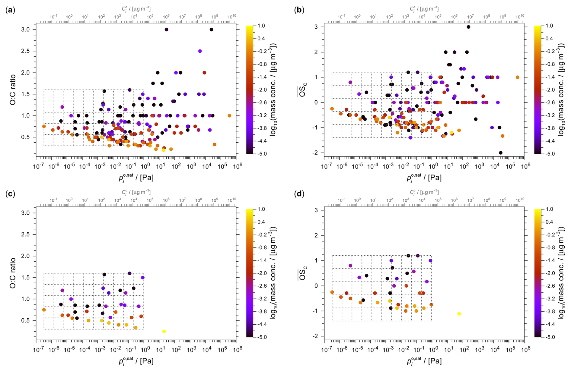
Figure 11 2D space representations of the α-pinene SOA system at 298 K using (a, c) the O:C ratio or (b, d) the mean carbon oxidation state as polarity axis. A 10×5 grid is shown in case of the full SOA system (a, b) as well as its use for the surrogate selection by the weighted medoid method (c, d).

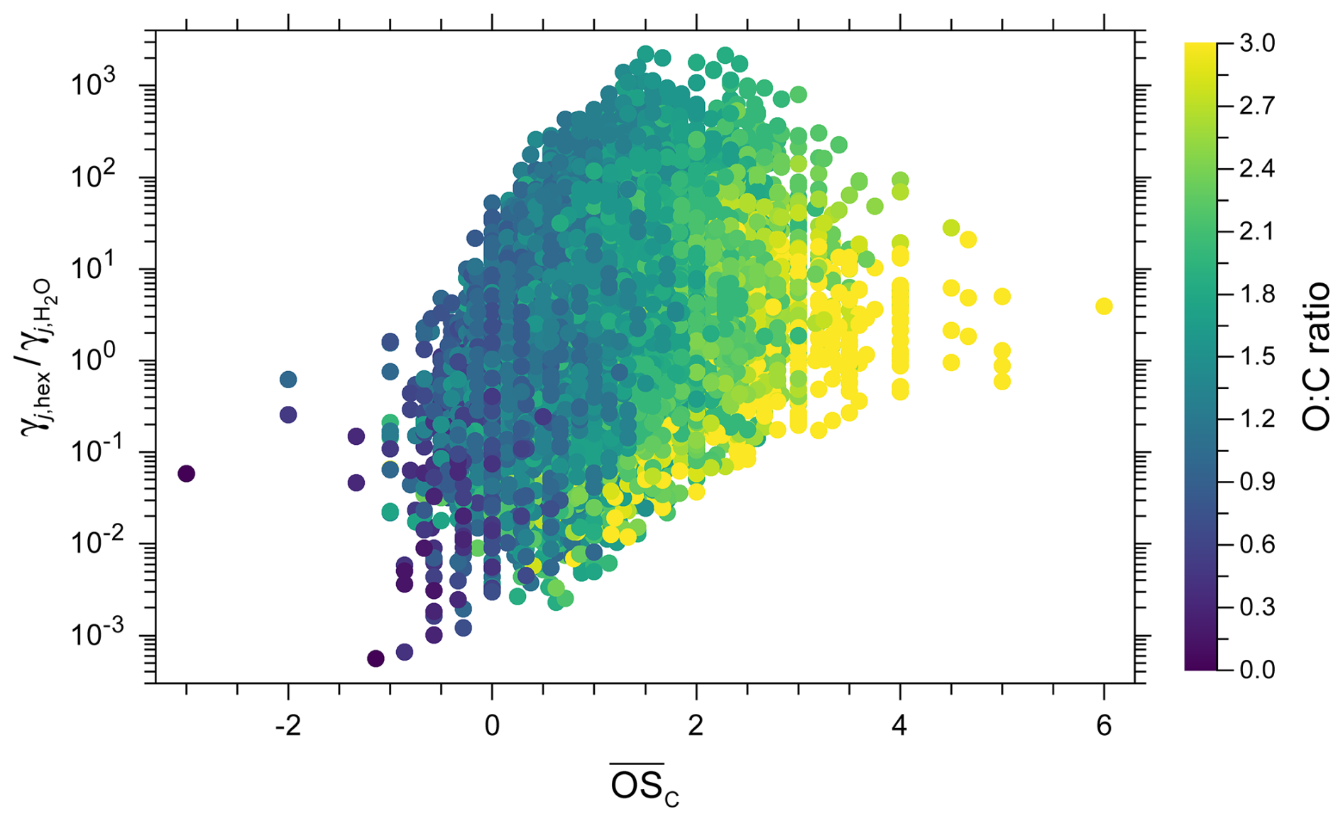
Figure 12 Comparison of three polarity axis metrics: ${\stackrel{\mathrm{‾}}{\text{OS}}}_{\mathrm{C}}$, ACR and O:C ratio for all components of the toluene SOA system. Both ${\stackrel{\mathrm{‾}}{\text{OS}}}_{\mathrm{C}}$ and ACR account for the impact of nitrogen-containing functionalities in a molecule on the respective metric, while the O:C ratio does not.

The accuracy of the grid-based and clustering approaches, as measured by MPE and MAPE, varies notably depending on the surrogate selection method and grid resolution chosen; refer to Tables 2–5. This variability underscores the importance of selecting appropriate methods for specific modelling objectives. At high resolutions, e.g. 10×5, the polarity axis choice has a modest impact, while it can be substantial at lower resolutions, especially in terms of predicted κ values when using the O:C polarity axis paired with one of the non-weighted gridded surrogate selection methods, in which case MAPE>50 % can occur.

In the case of the α-pinene system (Tables 2 and 3), the grid-based methods generally exhibit higher MAPE compared to the clustering-based k-means approach, especially at lower resolutions. This trend is consistent across the evaluated metrics and resolutions, highlighting the potential limitations of the simpler grid-based techniques in accurately reducing and representing complex chemical systems. Higher resolutions typically yield lower MAPE, especially in case of the two mass-weighted surrogate selection methods, indicating improved accuracy and preference in applications.

Overall, the activity coefficient ratio as polarity metric choice slightly outperformed the O:C ratio and the ${\stackrel{\mathrm{‾}}{\text{OS}}}_{\mathrm{C}}$ in case of the systems studied, demonstrating its ability in representing polarity in the context of subsequent gas–particle partitioning impacts on aerosol mass and hygroscopicity. In the case of the α-pinene system, the mass-weighted k-means approach using ACR achieved impressively low MAPE values, ranging from 2.0 % (4×2 resolution) to 0.1 % (10×5 resolution). The toluene system also showed good performance of the mass-weighted k-means approach with ACR, with MAPE values ranging from 6.0 % (4×2 resolution) to 4.3 % (10×5 resolution).

In a comparison of the different surrogate selection methods, the mass-weighted k-means method consistently scored as the most consistent and accurate across both systems. This is evident in case of the α-pinene SOA system when using the O:C ratio for polarity. The mass-weighted k-means method demonstrated superior performance with low MAPE values (0.2 % to 6.7 %) for predicted SOA mass concentrations across various system resolutions. In contrast, the midpoint method showed significant variability, with the MAPE ranging from 6.6 % to 51.2 %. The medoid and weighted medoid methods also displayed lower consistency with the MAPE reaching up to 39.8 %. In terms of the predicted hygroscopicity parameter of the α-pinene SOA, MAPE values spanned from 0.0 % (high resolution, ACR, k-means method) to 89.1 % (low resolution, O:C ratio, medoid method).

In the case of the toluene SOA system using the O:C ratio, k-means performed again well and consistently accros different resolutions in terms of predicted SOA mass concentrations, with MAPE values ranging from 1.3 % to 4.9 %. The other surrogate selection methods showed higher variability, with MAPE values of up to 13 % in case of the midpoint method at 4×2 grid resolution. Although, we note that a MAPE of 13 % could still be considered a good performance compared to uncertainties in field measurements of mass concentrations and aerosol composition. The predicted κ values for the toluene system showed a broader range of MAPE values, in the case of the O:C ratio axis ranging from 1.0 % (weighted medoid, highest resolution) to 143 % (midpoint method, lowest resolution) and substantial MPE variability (−143 % to +131 %), indicating significant over- and under-predictions by different methods at the lowest grid resolution studied (4×2).

When using the ${\stackrel{\mathrm{‾}}{\text{OS}}}_{\mathrm{C}}$ metric, the mass-weighted k-means method again outperformed alternative approaches at most resolutions. In case of the α-pinene SOA system, k-means resulted in MAPE values ranging from 0.9 % to 1.7 % for predicted SOA mass concentrations across various grid resolutions, approximately as accurate as with the ACR polarity axis. The other surrogate selection methods exhibited higher variability, with the midpoint method showing MAPE values as high as 71.4 % for the 4×2 grid resolution. For the predicted κ values, MAPE ranges from 2.5 % (k-means) to 36 % (midpoint method).

In the case of the toluene SOA system, using ${\stackrel{\mathrm{‾}}{\text{OS}}}_{\mathrm{C}}$, the k-means method continued to perform well and consistently, with a MAPE between 0.8 % and 4.7 % for predicted SOA mass concentrations. The other methods showed relatively good performance as well, with a maximum MAPE of 11 % (weighted medoid method, 4×2 grid resolution). In terms of the predicted SOA κ, MAPE values ranged from 8.5 % to 90 %, and MPE values spanned from −49 % (k-means, 6×3 resolution) to 90 % (medoid, 8×4 resolution), again showing higher variability in case of this metric, even when using the mass-weighted k-means method (MAPE from 10 % to 70 %). In comparison, when using ACR as polarity axis, the k-means method achieves a worst MAPE for κ of 31 % for the 4×2 resolution – approximately equivalent to the MAPE of 30 % for an 8×4 resolution when using ${\stackrel{\mathrm{‾}}{\text{OS}}}_{\mathrm{C}}$ for polarity. This is also consistent with ACR leading to better k-means performance compared to ${\stackrel{\mathrm{‾}}{\text{OS}}}_{\mathrm{C}}$ in case of the α-pinene SOA system.

4 Conclusions

This study introduces a novel chain of computational tools to advance the prediction of organic aerosol formation, which can be applied to chemical product evolution predictions from near-explicit gas phase mechanisms. This will allow the community to approach atmospheric chemistry modelling of organics and related aerosol composition and mass concentrations at a highly detailed level. A level that is only accessible with the aid of automatic product classification methods. By integrating structure- and system-level tools, our work paves the way for gas–particle partitioning modelling involving large numbers of aerosol components, a challenge that has long hindered highly detailed system studies on SOA formation and composition.

The developed suite of automated tools, including the SMILES to AIOMFAC Subgroups tool (S2AS), enhances processing capabilities for complex chemical systems, as demonstrated for compounds resulting from α-pinene ozonolysis or toluene oxidation. The introduction of a scalable 2D framework with grid-based and cluster-based surrogate selection methods, represents a major advancement in simplifying complex chemical systems while maintaining controllable accuracy in SOA partitioning predictions and retaining structural information (of the surrogates).

The evaluation of the framework's applications to two SOA systems provided information about the effects of polarity axis choices and system resolution. We examined the impact of choosing relatively low to moderate grid resolutions (4×2, 6×3, 8×4, 10×5) in surrogate representations of gas–particle systems. As expected, higher grid resolutions (or higher number of k-means clusters) generally yield better accuracy at the cost of increased computational cost for the gas–particle partitioning computation step. By reducing the number of species from hundreds or thousands to just ∼32 surrogate components, substantial computational efficiency gains were achieved without compromising accuracy in SOA mass predictions substantially. Based on the two example systems discussed, we recommend grid resolutions of at least 8×4 to maintain expected prediction errors within a 10 % threshold. More generally, for reference offline gas–particle partitioning computations in which computational costs are secondary concern, we recommend choosing the highest grid or cluster resolution feasible for the use case, up to about 200 surrogate components. Beyond 200 surrogate components, the cost versus accuracy trade-off will likely result in diminishing returns in terms of improvements in predicted (aerosol) system properties.

Our quantitative analysis highlights the effectiveness of the mass-weighted k-means method. When it is applied with the ACR polarity representation, good performance is achieved even at relatively coarse resolutions of an organic aerosol system. The choice of polarity axis metric impacted the accuracy and consistency of SOA system representation. Compared to the O:C ratio and ${\stackrel{\mathrm{‾}}{\text{OS}}}_{\mathrm{C}}$ proxies for polarity, the ACR metric is particularly effective since it encodes more information about a components structure and mixing properties in aqueous SOA. The k-means based medoid approach paired with the ACR metric emerged as the most effective 2D lumping and surrogate selection method among those evaluated. While it may be possible to improve the grid-based surrogate selection methods, e.g. by introducing variable-resolution grids with higher resolution in the semivolatile range, the strong performance of the k-means method renders such improvements unnecessary.

We envision a few distinct options for future applications of this framework in different kinds of atmospheric chemistry models. (1) Within detailed chemical box or plume models, those that consider a large number of compounds and retain their molecular structure information, the computation of surrogates and subsequent gas–particle partitioning at each desired (output) time step may be the preferred option. (2) Alternatively, based on a separate offline calculation for a specific system, a fixed set of surrogate compounds could be determined with the 2D framework. Subsequently, at each time step, existing and newly formed compounds from the box model's chemical mechanism could be mapped to this conserved, predetermined set of surrogates using the closest normalized Euclidean distance to the various surrogates in the 2D space (similar to Eq. 6) to determine the surrogate to which a compound's mass will be lumped. (3) In the case of simplified chemical mechanisms, such as those often employed in large-scale chemical transport models, maintaining only a few organic aerosol surrogates or a 1D/2D VBS representation, the application differs since surrogate lumping during simulations is unnecessary. In that case, the 2D framework could serve in systematically generating sets of surrogate components after mechanism simulations (e.g. with GECKO-A) for targeted aerosol precursors (structure-resolved) or aid in generating 2D VBS bin-resolved (structure-agnostic) representations at desired polarity–volatility resolutions. In the latter case, the 2D lumping step may serve in assigning surrogates in the ACR vs. p° space and in translating the resulting surrogate mass concentrations into bin-based mass concentrations, e.g. in the O:C vs. C° coordinate space. In the case of atmospheric chemistry models that retain the molecular structure information of surrogates, we envision two options for invoking equilibrium gas–particle partitioning calculations during simulations. (i) Applying the gas–particle partitioning calculation offline at specific output times during a simulation while running the gas-phase chemical mechanism as if all material remained in the gas phase (no feedback from partitioning). (ii) Running the 2D lumping framework and the gas–particle partitioning method at every simulation time step, followed by treating the determined fractional surrogate amounts partitioned to the particle phase as partially or fully shielded from further gas-phase chemical reactions. The gas-phase fraction of a surrogate would then be applied to the list of associated compounds, updating their molecular gas-phase concentrations prior to the next chemical reaction step in the simulation. Optionally, reactions in the condensed phase could be treated separately by a distinct mechanism.

A computationally effective use of near-explicit gas-phase chemical mechanisms in atmospheric chemistry models benefits often from a tunable reduction in the complexity of the mechanism itself, both in terms of number of explicit species and number of reactions covered. Methods such as the GENerator of reduced Organic Aerosol mechanism (GENOA) (Wang et al., 2022) and the Automated MOdel REduction (AMORE) algorithm based on graph theory (Wiser et al., 2025) serve this purpose. When targeting SOA formation applications, AMORE v2.0 employs a 2D categorization based on the saturation vapour pressures and Henry's law constants of organic components, which is similar to the polarity–volatility space of our 2D framework. Further development of such rule-based mechanism reduction methods may therefore benefit from considering also our 2D framework for potential application in compound classification.

In conclusion, the introduced computational framework will aid in bridging the wide gap between detailed, molecular-level reaction and simulation mechanisms and the computationally constrained, much simpler aerosol schemes of regional and large-scale atmospheric models. It provides automated tools and lumping techniques for generating reduced-complexity representations of aerosol properties and gas–particle partitioning inputs in a systematic and objective manner. Furthermore, the scalability of the 2D framework allows researchers to adjust the level of detail based on specific research needs while being mindful of computational constraints. Alongside with detailed chemical mechanisms, such as GECKO-A, future work could make use of the introduced tools in simulations of specific environmental chamber studies on aerosol formation from known precursors – and to represent related gas–particle systems by a tuneable selection of structure-resolved surrogates.