An improved modelling chain for bias-adjusted high-resolution climate and hydrological projections for Norway

About every 10 years, the Norwegian Centre for Climate Services publishes a national climate assessment report, presenting the updated historical climate change and climate projections towards the end of this century. This paper documents the model experiment used to generate high-resolution climate and hydrological projections for the new climate assessment report published in October 2025. The model experiment follows the standard modelling chain for hydrological impact assessment, i.e., climate model selection – downscaling and bias adjustment – hydrological modelling. However, compared with the model experiment for the climate assessment report published in 2015, all modelling components have been improved in terms of data availability, data quality and methodology. Specifically, a large climate model ensemble was available and new criteria were developed to select tailored climate projections for Norway. Two bias-adjustment methods (one univariate and one multivariate) were applied to account for the uncertainty of method choice. The hydrological modelling was improved by implementing a physically-based Penman–Monteith method for evaporation and a glacier model accounting for glacier retreat under climate change scenarios. Besides model description, this paper elaborates the effects of different bias-adjustment methods and the contribution of climate models and bias-adjustment methods to the uncertainty of climate and hydrological projections under the RCP4.5 scenario as examples. The results show that the two bias-adjustment methods can contribute larger uncertainty to seasonal projections than climate models. The multivariate bias-adjustment method improves hydrological simulations, especially in the reference period, but cannot conserve climate change signals of the original climate projections. The dataset generated by the presented modelling chain provides the most updated, comprehensive and detailed hydrometeorological projections for mainland Norway, serving as a knowledge base for climate change adaptation to decision makers at various administrative levels in Norway.

1 Introduction

It is unequivocal that human influence has warmed the climate at a rate that is unprecedented in at least the last 2000 years (IPCC, 2023). The human-induced warming has already modified the global hydrological cycle, leading to significant shifts in the spatial and temporal patterns of hydrological components (Gu and Adler, 2015; Gudmundsson et al., 2021; Li et al., 2023) and more intensive and frequent hydroclimatic extreme events (Alifu et al., 2022; Chinita et al. 2021; Dunn et al., 2020; Padrón et al., 2020). These impacts pose unprecedented challenges for water resource management at regional and local scales, and they are expected to be more severe in the future if unsustainable development continues (Wang and Liu, 2023). Therefore, understanding of the potential climate change impact from a long-term and systematic perspective serves as a key basis to develop climate adaptation strategies, such as incorporating climate projections into European building standards (EEA, 2025) and national climate risk adaptations (DCCEEW, 2023).

General circulation models (GCMs) are important tools to understand and predict climate behavior under various greenhouse gas emission scenarios on the global scale. GCMs have been developed rapidly in the last decades, with an increasing number of models from over 40 within the Coupled Model Intercomparison Project phase 5 (CMIP5, Taylor et al., 2012) for Representative Concentration Pathway (RCP) emission scenarios to over 60 within CMIP6 (Eyring et al., 2016) for the Shared Socioeconomic Pathways (SSP) emission scenarios. Such a large ensemble of models provides valuable information of uncertainty for future climate projections, accounting for natural climate variability, unknown socio-economic developments, and model differences (Hawkins and Sutton, 2011). However, the use of the full ensemble can be challenging for impact models due to computational restrictions, so it often requires a careful selection of projections for specific study areas based on comprehensive analysis of the whole ensemble (Dalelane et al., 2018). In addition, GCM outputs are hardly applied for impact assessment at regional and local scales due to their coarse spatial resolutions (e.g., ∼ 0.25 to 3° for the CMIP6 models and ∼ 0.5 to 4° for the CMIP5 models) and systematic biases (Rössler et al., 2019), and they are usually downscaled to fine spatial resolutions and bias adjusted for climate impact assessment and adaptation planning (Martinich and Crimmins, 2019).

The GCM outputs can be downscaled dynamically using regional climate models (RCMs) or statistically based on statistical relationships between coarse-resolution variables in GCMs and fine-resolution or local observations in the historical period (Zhang et al., 2020). Various RCMs and statistical downscaling methods have been developed and applied to downscale the GCM outputs, increasing the number of climate projections for region scales. For example, the European Coordinated Regional Downscaling Experiment (EURO-CORDEX, Jacob et al., 2020) applies 11 RCMs to downscale the outputs from 14 GCMs to 0.11° (ca. 12.5 km) horizontal resolution. Due to the high computational cost and time consumption, each RCM is able to downscale one or a few GCMs outputs, resulting in 30, 25 and 64 regional climate projections for Europe under the RCP2.6, RCP4.5 and RCP8.5 scenarios, respectively. In contrast, statistical downscaling methods, which are often combined with bias adjustment, can be easily applied for a large ensemble of GCMs due to low computational requirements and fast calculations, and over 50 statistical downscaling methods have been applied for Europe (Gutiérrez et al., 2019).

Each downscaling method has its strengths and weaknesses. The dynamic downscaling ensures the physical relationships between climatic variables and spatial dependence, but it inherits significant biases from GCMs and requires further bias adjustment and/or statistical downscaling depending on the scale of impact studies (Hundecha et al., 2016; Maraun and Widmann, 2018). In contrast, the statistical downscaling usually outperforms the RCMs in terms of bias, but many methods downscale individual climatic variables independently. As univariate bias-adjustment methods, this approach does not modify inter-variable dependency structures but keeps them as in the original model data which can be inaccurate. Eum et al. (2020) demonstrated different impact of univariate and multivariate statistical downscaling methods on reproduction of snowfall and recommended the use of the multivariate methods for climate change impact assessment in snow-dominated watersheds. Meyer et al. (2019) also found underestimation of snow accumulation (up to 50 %) in alpine catchments when using univariate contra multivariate bias-adjustment approach, which can be attributed to less precipitation below temperatures of 0 °C.

Due to the large number of GCM projections and downscaling methods, as well as their strengths and weaknesses, to construct a downscaled and bias-corrected ensemble for specific regions is challenging. Different choices of GCM and downscaling methods can lead to considerably different local climate projections and thus contribute large uncertainty to local decision-relevant climate outcomes (Tang et al., 2016; Lafferty and Sriver, 2023). In addition, they result in different climate impact projections for streamflow (Kay, 2025), flood hazard (Kundzewicz et al., 2017), agriculture (Li et al., 2023), ecosystem (Pourmokhtarian et al., 2016), etc, causing inconsistent impact assessments not only within each impact sector but also across sectors. Therefore, a consistent and tailored ensemble of regional climate projections is highly appreciated for each region and many countries have put great efforts to create national ensembles of climate projections (Golding et al., 2025), such as Switzerland (Fischer et al., 2022), Germany (Hübener et al., 2017), UK (Reyniers et al., 2025) and Australia (Peter et al., 2024).

Norway is located in the northern high latitudes, which have experienced the strongest warming since 1980 among all regions in the world, with warming trends spanning from 0.2 to more than 0.6 °C decade⁻¹ (IPCC, 2023). The strong warming in the historical period raises great attention from both the scientific community and the public to future climate change and its impacts on hydropower production (about 90 % of total power production in the country), winter tourism (skiing), and water related natural hazards (i.e., flood, drought, avalanche and landslide). However, it is specifically challenging to construct robust and reliable climate projections as well as hydrological impact projections in Norway, due to the high heterogeneity in topographic and hydroclimatological characteristics.

Norway is one of the most mountainous countries in Europe, with more than 90 % of the landscape consisting of mountains. The rugged topography leads to a complex spatial and temporal pattern of temperature and precipitation, varying with geographical position, elevation, aspect (slope direction), and slope angle (Dobrowski et al., 2009; Franke, 2024). The spatial resolutions of the state-of-the-art GCMs and RCMs are too coarse to provide sufficient spatial variations of climate for such complex terrain. In addition, these projections often show a cold bias for Norway (Wong et al., 2016), which for example leads to a prolonged snow season, low winter runoff and late snowmelt in hydrological projections (Nilsen et al., 2021).

In order to construct a consistent and tailored ensemble of national climate projections as well as hydrological projections for Norway, the Norwegian Centre for Climate Services (NCCS) brings together experts from the Norwegian Meteorological Institute, the Norwegian Water Resources and Energy Directorate (NVE), the Norwegian Research Centre (NORCE) and Bjerknes Centre for Climate Research. NCCS is responsible for the national climate assessment report, updated about every 10 years, which presents updated historical climate change and climate projections towards the end of this century and serves as a knowledge base for climate change adaptation to decision makers and planners at various administrative levels in Norway (Nilsen et al., 2022). The previous climate assessment report “Climate in Norway 2100” (Hanssen-Bauer et al., 2015; hereafter abbreviated CiN-2015), published in 2015, was based on 10 available GCM-RCM combinations within the CMIP5 and EURO-CORDEX frameworks. The projections were further re-gridded and bias-adjusted into 1 km × 1 km resolution using empirical quantile mapping and forced the distributed version of the HBV (Hydrologiska Byråns Vattenbalansavdelningen, i.e. “The Hydrological Bureau's Water Balance Department”) hydrological model (distHBV, Beldring et al., 2003) to generate hydrological projections. This spatial resolution is the result of the need to serve projections that can be used locally on the one hand, and availability of computational resources and reference datasets to produce daily maps for the whole of Norway on the other. During the last 10 years, all methods along the modelling chain, including GCMs, RCMs, climate model selections, statistical downscaling and bias correction, and hydrological models, have been further developed, and the observation data has been updated and improved. These developments promote the new generation of high-resolution and bias-adjusted climate and hydrological projections, which are more robust than the previous ones in CiN-2015.

In this paper, we present the full description of the methods to produce the updated downscaled and bias-adjusted climate projections and hydrological projections for the new climate assessment report for Norway “CiN-2025” (Dyrrdal et al., 2025), specifically focusing on selection of GCM-RCMs combinations, statistical downscaling and bias-adjustment and hydrological modelling. Section 2 introduces the study area and historical input data. The methods described include the overview of the whole modelling chain (Sect. 3), selection of atmospheric variables from a set of EURO-CORDEX simulations (Sect. 4), statistical downscaling and bias-adjustment method (Sect. 5) and hydrological modelling (Sect. 6). In Sects. 7 and 8, we present the climate and hydrological products and uncertainty analysis. Finally, we discuss the limitations of the methods and the potential applications of the products, and point out the way towards the next generation of national climate projections for Norway in Sect. 9.

2 Study area and historical data

2.1 Study area

The modelling domain of this study is the mainland of Norway and a few river catchments draining from neighbouring countries (Sweden and Finland) (Fig. 1), resulting in 354 448 1 km × 1 km grid cells. Due to large variations in latitude and altitude, Norway exhibits six climate regimes according to the Köppen–Geiger climate classification (Beck et al., 2018), ranging from temperate climate along the west coast to polar climate in high mountains and in the north (Fig. 1). The average elevation of Norway is about 460 m, ranging from 0 along the coast to 2469 m at Galdhøpiggen in the center of the country. Open firm ground and forest are the two major land covers in Norway, accounting for 36 % and 37.8 % of the mainland area, respectively (Statistics Norway, 2025). There are also large areas of bedrock (8.5 %), followed by water (6.2 %), bogs (5.4 %), agricultural land (3.5 %) and built-up (1.7 %). About 1 % of mainland Norway is covered by glaciers (Fig. 1). The mean annual temperature in the current standard normal period 1991–2020 ranges from −9.5 to +9.5 °C (Tveito, 2021). The warmest areas are found in lower-lying areas in southern Norway, and particularly along the coast in the southwest, while the coldest areas are in the high mountains and inland areas of the north. Norway also exhibits large spatial variability in precipitation, ranging from 212 mm in southern parts of Northern Norway to 6130 mm close to the Ålfotbreen glacier in Western Norway. The wet areas along the west coast are exposed to migrating low pressure systems most often arriving from the west-southwest (Lutz et al., 2024).

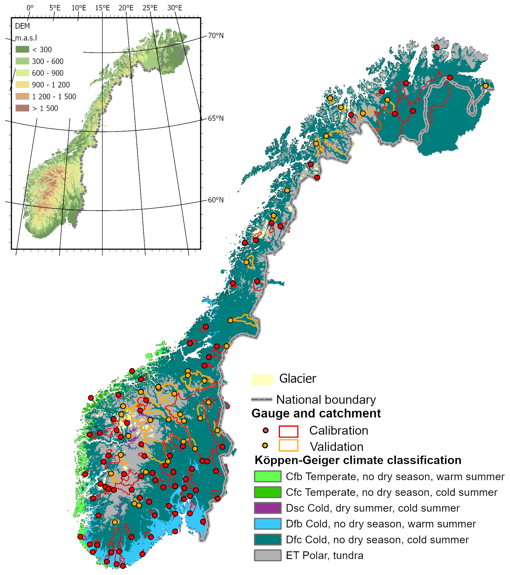
Figure 1 The climatic and topographic characteristics of the simulation domain as well as the locations of glaciers and hydrological gauging stations and catchment boundaries.

We selected 85 and 38 catchments for calibration and validation of the hydrological model, respectively. All these catchments are near-natural catchments and 112 of the 123 catchments are smaller than 1000 km². The distribution of the catchments represents various climate and hydrological regimes, geographic conditions and landscape types in Norway. The catchment boundary is delineated by NVE and the gauges at the outlet of these catchments are shown in Fig. 1.

2.2 Historical meteorological data

The historical meteorological data is used as reference in the bias-adjustment procedures and for hydrological model calibration and validations. It consists of nine atmospheric meteorological variables at a 1 km × 1 km grid covering Norway and river catchments in neighbouring countries (Fig. 1): mean, minimum and maximum 2 m temperature (K), precipitation flux (mm s⁻¹), relative humidity (%), longwave and shortwave radiation (W m⁻²), pressure (Pa) and 10 m wind speed (m s⁻¹).

Daily minimum, maximum and mean temperatures as well as precipitation are provided by the seNorge2018 v20.05 dataset (Lussana et al., 2019; Lussana, 2020). It covers the period 1957–2020 and is based on quality-assured daily datasets. The precipitation values are adjusted for wind-induced under-catch based on Wolff et al. (2015). Note that seNorge2018 continuously incorporates the latest available station data and is therefore not homogenized in time. This may affect the calculation of changes within the historical period.

Daily wind speeds for Norway from 1958 to 2020 are obtained from the KliNoGrid 16.12 dataset. The KliNoGrid dataset is based on the Norwegian atmospheric reanalysis NORA10 (Reistad et al., 2011) wind speed data, downscaled onto a 1 km grid using a quantile mapping approach (Bremnes, 2004) to match the climatology of the high-resolution numerical weather prediction model AROME-MEtCoOp (Müller et al., 2017).

Daily short- and longwave radiation, relative humidity and surface pressure are obtained from the HySN2018v2005ERA5 dataset. It is generated based on the ECMWF atmospheric reanalysis ERA5 (Hersbach et al., 2020) and seNorge2018 v20.05 and covers the period 1958–2020. The dataset is described in detail in Huang et al. (2022) and Erlandsen et al. (2021).

2.3 Data for setting-up hydrological models

To set up the hydrological model, a digital elevation model (DEM), as well as maps of soil type and land cover type with 1 km horizontal resolution are required. The DEM map was provided by the Norwegian Mapping Authority. Five soil types are reclassified based on the sediment map from the Geological Survey of Norway (Erlandsen et al., 2021), and bare mountain soil and moraine soils account for ca. 80 % of the total mainland area. Nine land cover types (open area, bog, built-up, forest, cropland, heather, bedrock, lake, permanent ice and snow) are classified based on the National Land Resource Map (Ahlstrøm et al., 2014) and the remote sensing based forest resource map SAT-SKOG (Gjertsen and Nilsen, 2012). The forest land cover is further classified into 12 structural forest types to distinguish three species groups (spruce, pine, and deciduous forest) and four forest development stages (underdevelopment, two intermediate development stages and mature forest) (Majasalmi et al., 2018). The parametrization for each forest structural type, such as maximum leaf area index, vegetation height and shortwave albedo, is given by Majasalmi et al. (2018) and Bright et al. (2018). For glacier areas, the glacier modelling doesn't account for variation of soil types and uses simplified land cover types including open area, bog, forest, bedrock and glacier area coverage. However, it requires glacier ice thickness and glacier area data (Andreassen et al. 2015) to setup the model.

Discharge measurements from 123 gauging stations are used to calibrate and validate the hydrological model (Fig. 1). They are quality-assured by NVE. All 123 stations have measured daily discharge from 1980 to 2014 with less than 5 % missing data. For the glacier modelling, mass balance data is only available for six glaciers and discharge measurements from 19 gauging stations downstream of the glaciers are used to calibrate and validate the hydrological model. All discharge and mass balance data are publicly available at https://sildre.nve.no (last access: 28 April 2026) and https://glacier.nve.no/glacier/viewer/ci/en/ (last access: 28 April 2026).

3 Modelling chain

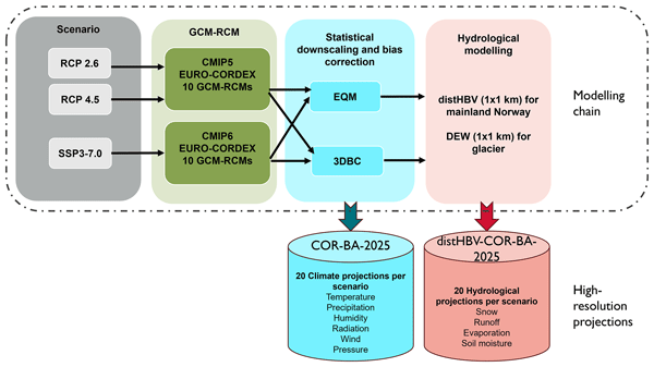
We followed the commonly used modelling chain in hydrological climate impact studies, i.e., (1) emission scenarios, (2) GCMs and RCMs, (3) statistical downscaling and bias correction and (4) hydrological model (Fig. 2). The first component of the modelling chain is to select emission scenarios. For the CiN-2025 report, two RCPs used in CMIP5 were selected, representing a very stringent pathway (RCP2.6) and a moderate-emissions pathway (RCP4.5). The shared socioeconomic pathway SSP3-7.0 used in CMIP6 was selected to represent the high-emission scenario. The reason why only one SSP scenario was selected is that SSP1-2.6 and SSP3-7.0 were the first-priority scenarios for the EURO-CORDEX community (Katragkou et al., 2024). The data has become available late with regard to the time needed to run our complete modelling chain – it is in fact still not openly available – making the selection of more than one SSP scenario infeasible. Such a combination of CMIP5 and CMIP6 scenarios has also been used in other national climate projections, e.g., the climate projections in Switzerland published at the end of 2025 (Schumacher et al., 2024) which combined EURO-CORDEX RCP8.5 with CMIP6 SSP5-8.5 GCM simulations.

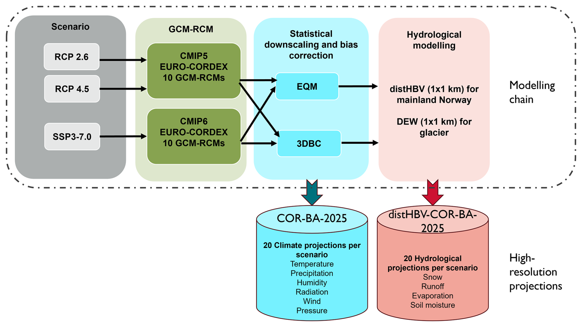
Figure 2 Modelling chain to generate high-resolution climate and hydrological projections for the CiN-2025 report.

In the second component of the modelling chain the task is to select a representative model ensemble from the EURO-CORDEX simulations (Jacob et al., 2014) for each emission scenario. Within the EURO-CORDEX framework, CMIP5 and CMIP6 GCMs are downscaled by different RCMs, resulting in a set of GCM-RCM combinations. For CiN-2025 a larger EURO-CORDEX ensemble for RCP scenarios was available compared to CiN-2015, enabling a more robust data basis and requiring new model selection strategies (Sect. 4).

Once the model ensemble was identified, the next step was to downscale the RCM projections of atmospheric variables from the original grid size of approximately 12.5 to 1 km. It was followed by removal of biases in RCM simulations relative to observed meteorological data (Sect. 2.2) in the calibration period. For future projections, we adjusted the values based on the corrections established in the calibration period under the assumption that the relationship between the observed and modelled data remains unchanged. Two bias-adjustment methods were used: de-trended empirical quantile mapping (denoted as EQM hereafter for simplicity) and three-dimensional bias-correction (3DBC) additionally to EQM (Sect. 5). The former is a widely used univariate bias-adjustment method and was used for CiN-2015. The latter adds a post-processing procedure, taking into account inter-variable dependencies. To our knowledge, this is the first time the 3DBC method is applied in Norway, and we have identified several strengths and weaknesses with this multivariate method (Sect. 5.3). Since the two bias-adjustment methods complement each other, we decided to apply both bias-adjustment methods on the RCM projections and provided two complete datasets (EQM only and EQM with 3DBC). To assess the uncertainty in the climate and hydrological projections from the choice of methods, we have carried out an uncertainty analysis (Sects. 7.3 and 8.3).

The last component of the modelling chain is hydrological modelling. The distHBV model was still the main tool for simulating hydrological components under different climate scenarios for the CiN-2025 report, but two major improvements have been made since CiN-2015. The first improvement was to replace the temperature-based evaporation method with the Penman–Monteith equation in the distHBV model (Huang et al., 2019), because physical-based approaches, such as the Penman–Monteith method, consider more climatic variables and provide more robust changes in potential evaporation under climate scenarios than the empirical ones (McAfee, 2013; Tam et al., 2024). The second improvement was the use of Distributed Element Water balance model (DEW) (Beldring, 2008) for glacierized regions. Since distHBV was not able to simulate the changes in glacier area, glacier melt water can be unrealistically simulated under climate scenarios. In contrast, DEW is able to simulate glacier area, volume and surface elevation dynamically and thus gives more reliable hydrological projections under climate change for glacierized regions. Both models ran independently at 1 km spatial resolution and with daily time steps, but distHBV ran for all grid cells in Norway and DEW only ran for the grid cells covering glacierized regions. A postprocessing procedure was carried out to combine the distHBV and DEW outputs to generate final runoff projections for mainland Norway.

The modelling chain resulted in two datasets with a spatial resolution of 1 km × 1 km at daily time steps, which will be serving as the basis for climate impact assessment in mainland Norway. The first dataset is termed COR-BA-2025 (short for CORDEX-Bias Adjusted, updated in 2025), consisting of 20 bias-adjusted high-resolution climate projections for each emission scenario and is available from 1970 to 2100 (2098 depending on GCMs). These projections include nine atmospheric variables at 1 km × 1 km spatial resolution and with daily time steps, each bias-adjusted both with EQM and 3DBC: mean, minimum and maximum 2 m temperature (K), precipitation flux (mm s⁻¹), relative humidity (%), longwave and shortwave radiation (W m⁻²), surface air pressure (Pa) and 10 m wind speed (m s⁻¹). The second dataset is called distHBV-COR-BA-2025 and consists of 20 hydrological projections for each emission scenario at the same spatial and temporal resolution and coverage as the atmospheric projections. The hydrological projections include two flux variables (runoff and evaporation) representing average values over each grid cell in mm d⁻¹, and two state variables (soil moisture and snow water equivalent), which describe the average condition of the hydrological components in a grid cell with unit mm. The evaporation, soil moisture and snow water equivalent projections were generated by distHBV, whereas the runoff projections were obtained by superimposing the results of the glacierized grid cells from the DEW model on the runoff projections from distHBV.

To select the climate ensembles and assess future changes in climate and hydrology, we defined one reference period (1991–2020) and two future periods (2041–2070 and 2071–2100). The reference period was selected by two factors: (1) a recent climate period better represents today's climate, and (2) 1991–2020 is the current standard normal period defined by the World Meteorological Organization (WMO). However, in CMIP5 and CMIP6, the historical simulation runs end in 2005 and 2014, respectively. Data from the emission scenario RCP4.5 was used to extend the historical period beyond 2005 for RCPs and the data from the emission scenario SSP3-7.0 was used to extend the historical period beyond 2014 for SSPs.

Table 1 Summary of the 17 GCM-RCM combinations available for RCP2.6, RCP4.5 and RCP8.5. Combinations in bold were selected for downscaling and bias-adjustment for the mainland of Norway.

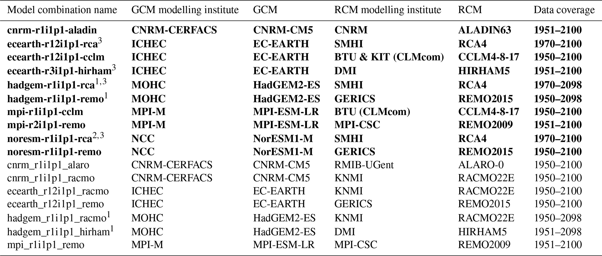
¹ Original data has 360 d only. Additional days added. ² Leap-year days added. ³ Spatial smoothing applied to tasmin, tasmax, tas and hurs.

Since the main focus of this paper is on the description of the methods in the modelling chain rather than assessing climate and hydrological projections under different emission scenarios, we mainly present the methods and results for the RCP4.5 scenario as examples in the following sections. However, the methods described in this paper are valid for all three scenarios.

4 Selection of GCM–RCM combinations

Currently, the EURO-CORDEX CMIP5 projections comprise the largest high-resolution regional climate model ensemble for Europe and Norway with more than 30 simulations based on RCP2.6, more than 20 simulations based on RCP4.5 and more than 70 simulations based on RCP8.5. However, there are (only) 17 model combinations covering all three RCPs (Table 1). To be able to do a proper comparison between future projections of different RCPs, it is important to use identical model combinations for each RCP. These identical model combinations comprise five GCMs, namely CNRM_CM5, EC_EARTH, HadGEM2-ES, MPI-ESM-LR and NorESM1-M. Given time and computational constraints, we defined an upper limit of ten model combinations that are used as forcing data for the hydrological models, thus seven model combinations had to be excluded.

As a first quality check we used Table 6 in McSweeney et al. (2015) to see if the five GCMs perform satisfactorily in the representation of two out of the three physical phenomena consisting of (i) annual temperature and precipitation cycles, (ii) circulation and (iii) storm tracks. This criterion did not lead to any exclusion of the 17 model combinations. As a next check we verify if the GCM-RCM combinations are ranked in the “best half” for 24 variables and impact-based indices (Table 2 in Vautard et al., 2021) for the region of Scandinavia (Fig. 12a in Vautard et al., 2021). This made us exclude cnrm _r1i1p1_alaro. Further, we excluded three simulations performed with the RCM RACMO22E which are affected by a bug in the snow albedo which again strongly affects the temperature signal above and around glaciers. This bug is documented in the EURO-CORDEX Errata table. Lastly, we checked the GCM-RCMs' performance with respect to the observed temperature and precipitation climate in Norway by using the seNorge v20.05 dataset as reference data. The differences between the temperature biases in the remaining model combinations were found negligible. The largest precipitation biases (> 14 %) were found for the historical simulations with hadgem2_r1i1p1_hirham, mpi-r1i1p1_remo and ecearth-r12i1p1_remo, hence we excluded these simulations.

This leaves us with ten selected model combinations presented in Table 1. The projected changes in temperature and precipitation are shown for each model combination in Fig. 3. Based on the selected ten GCM-RCM combinations (coloured dots in Fig. 3), the projected changes in temperature and precipitation in Norway range from 1.2 to 2.8 °C and from −1 % to 9 % in the future period 2071–2100 relative to the reference period 1991–2020.

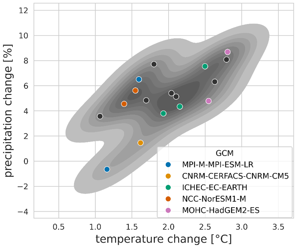
Figure 3 Projected changes in temperature and precipitation for mainland Norway by the end of the century relative to the reference period (1991–2020) under the RCP4.5 scenario (all dots). The grey shaded area indicates the distribution (kernel density estimate) of the projected changes comprising all 17 GCM-RCM combinations that were considered. The individual coloured points highlight the ten simulations selected for CiN-2025 (Table 1).

The selected GCM-RCM combinations vary in data coverage and quality (Table 1). The GCM HadGEM2-ES lacks 13 months towards the end of the time series, so we only used the simulations forced by this GCM until the end of 2098. When looking at near (2041–2070) and far future (2071–2100) changes, the HadGEM2-ES simulations were shifted by 2 years, i.e. the periods for HadGEM2-ES were 2039–2068 and 2069–2098. In addition, HadGEM2-ES driven EURO-CORDEX CMIP5 simulations use the HadGEM2-ES calendar with 360 d instead of 365 (366) days. To fill in the missing 5 d, we simply copied the day number 150, 210, 240, 300 and 360 from the 360 d year and added these extra days to the day number 151, 212, 243, 304 and 365 in a normal year. For a leap year, a copy of day number 59 was added similarly. This simple technique was also used on NorESM1-M coupled with RCA4 as this model combination does not support leap years. Unrealistically large snow accumulation at isolated grid cells have been discovered in the simulations from RCA4 and HIRHAM5. They were considered as minor quality issues and their effects were reduced by applying a spatial smoothing on the variables minimum, mean and maximum temperature, and humidity, an approach adopted from CH2018 (2018).

The selection criteria for the EURO-CORDEX CMIP6 projections are different from the ones for the EURO-CORDEX CMIP5 projections, because there were (only) 14 RCM simulations based on CMIP6 available by June 2024 (Table S1 in the Supplement). Also, a selection of CMIP6 GCMs providing a satisfactory performance over Europe and covering a reasonable part of the climate change signal had already been carried out for the EURO-CORDEX CMIP6 simulations by Sobolowski et al. (2025). The main criteria for the selection here were thus to include as many GCMs as possible, a balanced RCM selection and excluding model combinations that show fairly similar results in temperature and precipitation over Norway. This led us to exclude the model combinations ecearthveg_r1i1p1f1_icon, ecearthveg_r1i1p1f1_racmo and miroc_r1i1p1f1_hclim. We further excluded noresm_r1i1p1f1_racmo due to a low climate sensitivity and small precipitation changes during the summer months.

5 Downscaling and bias-adjustment methods

For CiN-2015, only daily mean temperature and precipitation were bias-adjusted, but for CiN-2025, nine surface variables from the RCM outputs were downscaled and bias-adjusted, namely mean, minimum and maximum air temperature at 2 d height, precipitation, mean wind speed at 10 m height, long- and shortwave radiation, surface pressure, and relative humidity at 2 m height.

The nine climate variables from the RCM outputs were firstly re-gridded to the seNorge grid with a 1 km spatial resolution using the nearest-neighbour method. This conservative way to downscale from a coarse to fine scale grid ensures that the original model outputs are preserved and not altered unintentionally by the downscaling step. The bias-adjustment procedure was then implemented on the grid cell basis. Depending on the variable adjusted, different reference datasets (see Sect. 2.2) were used for training.

Since the grid cells are bias-adjusted individually, we need to select methods that are computational efficient, or at least applicable, and numerically stable (François et al., 2020) for a large number of grid cells (354 448 in total). We have tested a few bias-adjustment techniques categorized as quantile mapping (Cannon et al., 2015) and multivariate approaches (François et al., 2020). In the end, the univariate bias-adjustment adopting de-trended empirical quantile mapping (EQM) approach (Bürger et al., 2013) was used to bias-adjust one climate variable at a time because the method meets all the aforementioned criteria and is widely used in adjusting climate model data. EQM is effective in removing the model biases, preserving the trend and climate change signal moments (i.e. mean and standard deviation) and estimating extremes. As no univariate method can correct the possible biases in correlation among the atmospheric variables, all the EQM results were further post-processed with the multivariate 3DBC approach (Mehrotra and Sharma, 2019) to rectify inter-variable, temporal and spatial dependency structures.

5.1 EQM

The EQM approach adopted in this study is a de-trended variant of quantile mapping method which first establishes a statistical transfer function for a variable between RCM outputs and reference data in the training period 1985–2014. Twelve calendar-month-specific transfer functions were derived by fitting the empirical cumulative distribution functions (eCDFs) of the modelled values with the eCDFs based on reference data for each grid cell. With these monthly bias-adjustments we correct model biases which are varying throughout the year. This is essential for instance to produce realistic seasonal flow patterns and hydrological regimes in the subsequent hydrological modelling. To avoid overfitting, daily data within a 3-month window centred on the month of interest were pooled and used to develop the monthly eCDFs (Cannon et al., 2015). For example, data from February to April were used to develop the eCDF for March.

The transfer functions were approximated by a series of empirical quantiles with fixed intervals of 0.01 spanning the probability space (0,1) (Gudmundsson et al., 2012). Only the 1st to 99th quantiles were obtained and used. Linear interpolation was applied for values in between those fixed quantiles. For values smaller than the 1st quantile and larger than the 99th quantile, linear extrapolation was performed based on the slopes derived from the 1st and 2nd quantiles and 98th and 99th quantiles, respectively. These functions are assumed to be applicable to the projection period.

Wet-day correction has also been applied prior to bias-adjustment of precipitation. In our study region, RCMs generally provide more rainy days than observed ones (see e.g. Lhotka et al., 2024). Thus, for each grid cell, a threshold value is derived such that the wet-day frequency in modelled precipitation is equal to that in the corresponding reference data for the training period. All modelled precipitation values which are below the derived threshold value are then set to zero for both training and projection periods (Gudmundsson et al., 2012).

To reduce the potential impact of over-adjustment (modifying the long-term linear trend) and extrapolation (model-projected values lying outside the range of the historical distribution), the long-term linear trend (usually 30-year) of the projected period was first removed from model projections. Scaling the range of future projection to align closer to the historical one improves the applicability of the transfer function by reducing the need to extrapolate beyond historical values, while the daily variability about the monthly mean remains unchanged. The trend was reimposed after the bias-adjustment of the residuals. For all the variables other than temperatures, trend removal and reimposition were performed multiplicatively, i.e. variability and residuals were considered as ratios rather than differences. The procedure was applied separately for twelve months. For example, for precipitation for month i, the scaling factor δP_i, which also represents the relative precipitation trend, is defined as:

$$\begin{array}{}\text{(1)}& \mathit{\delta }{P}_i={\stackrel{\mathrm{‾}}{P}}_i^{\text{prj}}/{\stackrel{\mathrm{‾}}{P}}_i^{\text{tng}}\end{array}$$

where ${\stackrel{\mathrm{‾}}{P}}_i^{\text{prj}}$ and ${\stackrel{\mathrm{‾}}{P}}_i^{\text{tng}}$ refer to mean monthly accumulated precipitation for month i for the projection and training periods, respectively. The de-trended daily precipitation in the projection period for a specific calendar month i (= January, February, …, December), ${\widehat{P}}_i^{\text{prj}}\left(t\right)$, is:

$$\begin{array}{}\text{(2)}& {\widehat{P}}_i^{\text{prj}}\left(t\right)=P_i^{\text{prj}}\left(t\right)/\mathit{\delta }{P}_i\end{array}$$

where $t=\mathrm{1},\mathrm{2},\mathrm{\dots },N_i$ is the time step, and N_i the number of days belonging to the calendar month i in the projection period. $P_i^{\text{prj}}\left(t\right)$ denotes the original RCM daily precipitation time series for month i in the projection period. EQM was applied to the de-trended time series, and the precipitation trend for month i was then re-introduced to the bias-adjusted de-trended results ${\stackrel{\mathrm{˘}}{P}}_i^{\text{prj}}\left(t\right)$ for month i. The bias-adjusted precipitation, ${\stackrel{\mathrm{̃}}{P}}_i^{\text{prj}}\left(t\right)$, for month i can be obtained by:

$$\begin{array}{}\text{(3)}& {\stackrel{\mathrm{̃}}{P}}_i^{\text{prj}}\left(t\right)={\stackrel{\mathrm{˘}}{P}}_i^{\text{prj}}\left(t\right)\cdot \mathit{\delta }{P}_i\end{array}$$

Similarly linear trend removal and reimposition for the projected values of temperature variables were done additively. Following similar notation, the temperature trend, δT_i, for month i simply equals to ${\stackrel{\mathrm{‾}}{T}}_i^{\text{prj}}-{\stackrel{\mathrm{‾}}{T}}_i^{\text{tng}}$, and the de-trended daily temperature, ${\widehat{T}}_i^{\text{prj}}\left(t\right)$, can be derived from:

$$\begin{array}{}\text{(4)}& {\widehat{T}}_i^{\text{prj}}\left(t\right)=T_i^{\text{prj}}\left(t\right)-\mathit{\delta }{T}_i\end{array}$$

where $T_i^{\text{prj}}\left(t\right)$ represents the original RCM daily temperature for month i in the projection period. The bias-adjusted temperature for month i, ${\stackrel{\mathrm{̃}}{T}}_i^{\text{prj}}\left(t\right)$, can be recovered by adding the temperature trend δT_i to the bias-adjusted de-trended data ${\stackrel{\mathrm{˘}}{T}}_i^{\text{prj}}\left(t\right)$:

$$\begin{array}{}\text{(5)}& {\stackrel{\mathrm{̃}}{T}}_i^{\text{prj}}\left(t\right)={\stackrel{\mathrm{˘}}{T}}_i^{\text{prj}}\left(t\right)+\mathit{\delta }{T}_i\end{array}$$

The projection period starting from 2015 to 2100 was further divided into seven overlapping 30-year time slices. The first time slice, however, only covers 2015–2040, followed by 2021–2050, 2031–2060, etc. After the bias-adjustment of each time slice using the established monthly transfer functions, only the 10-year results in the middle of the period were being kept. This procedure can better preserve the decadal trend but at the same time might introduce discontinuities in the time series at the start of each decadal period. The impact of such jumps in e.g. temperature might affect the snow accumulation in hydrological modelling at the transitions between the decadal periods. On the other hand, such jumps are negligible when the focus is on overall 30-year statistics. The impact of this approach is also expected to be smaller than shifting the entire 30-year window in each iteration. This is a pragmatic way to handle a basic limitation of the method. For the first and the last time slices, the results of the first 16 years and the last 20 years were used, respectively. A continuous time series covering the whole projection period was put together afterwards.

5.2 3DBC

The bias-adjusted climate projections based on the univariate EQM approach show the same dependency structures as the uncorrected RCM simulations. To impose inter-variable, temporal and spatial dependency structures obtained from the reference datasets, an additional post-processing step has been applied. The multivariate method we used for this is called 3DBC (three-dimensional bias-correction) as it adjusts along the three dimensions: variables, time and space. It is described in detail in Mehrotra and Sharma (2019). 3DBC is re-establishing the spatial, temporal and inter-variable structures from the reference data by reordering the daily EQM values according to observed time-ranks at each grid-point, resulting in the bias-adjusted data having the same rank structure (ordering) as the reference data in the calibration period. Compared to other multivariate bias correction methods (e.g. the MBCn method developed by Cannon, 2018) the computational requirements of 3DBC are relatively small, making its application on a large number of grid cells feasible. Note that 3DBC adjusts the ranks for future periods according to changes in the temporal auto-correlations as simulated by the RCMs. Thus, it does not strictly assume that the dependency structures remain stable in future climates. However, while the original implementation by Mehrotra and Sharma (2019) works on single calendar days across a future period of 30 years, our future period (2021–2100) consists of 80 years. Following the original approach would have resulted in imposing observed trends repeatedly on the future period. We thus adapted the 3DBC method to work within single years of the EQM data, an approach that maintains the climate change signals and trends from the RCMs (and EQM) on an annual scale. As a result, the adjustments in the variable auto-correlations for the future periods have a limited effect and do not fully transfer the dependency structure changes from the RCMs to the 3DBC bias-adjusted data. Since 3DBC reshuffles the bias-adjusted times series resulting from EQM within a year, the marginal distributions at seasonal scale might be modified.

5.3 Evaluation of bias-adjustment methods

5.3.1 Performance of bias-adjustment methods

Thorarinsdottir et al. (2013) proposed the use of integrated quadratic distance (IQD) as a performance measure to compare the full distribution of climate model output to the corresponding distribution of observed data. IQD was further employed by Yuan et al. (2019, 2021) to assess the performance of different bias-adjustment approaches. IQD (Eq. 6) is defined as:

$$\begin{array}{}\text{(6)}& d_{\text{IQ}}(F,G)={\int }_{-\mathrm{\infty }}^{+\mathrm{\infty }}\left(F\right(t)-G(t){)}^{\mathrm{2}}\mathrm{d}t\end{array}$$

where F, G are two cumulative distribution functions. d_IQ(F,G) summarizes the differences, and a lower value implies a smaller difference between F and G. $d_{\text{IQ}}(F,G)=\mathrm{0}$ if F=G. For further details, please see Thorarinsdottir et al. (2013). In this study, we compared the eCDFs of bias-adjusted precipitation and temperature with corresponding seNorge2018 v20.05 data over the training (1985–2014) and validation (1960–1984 or 1970–1984 depending on the period start of the RCM) periods in each grid cell. In addition, we calculated IQD scores derived from comparison of original RCM outputs with the observed data.

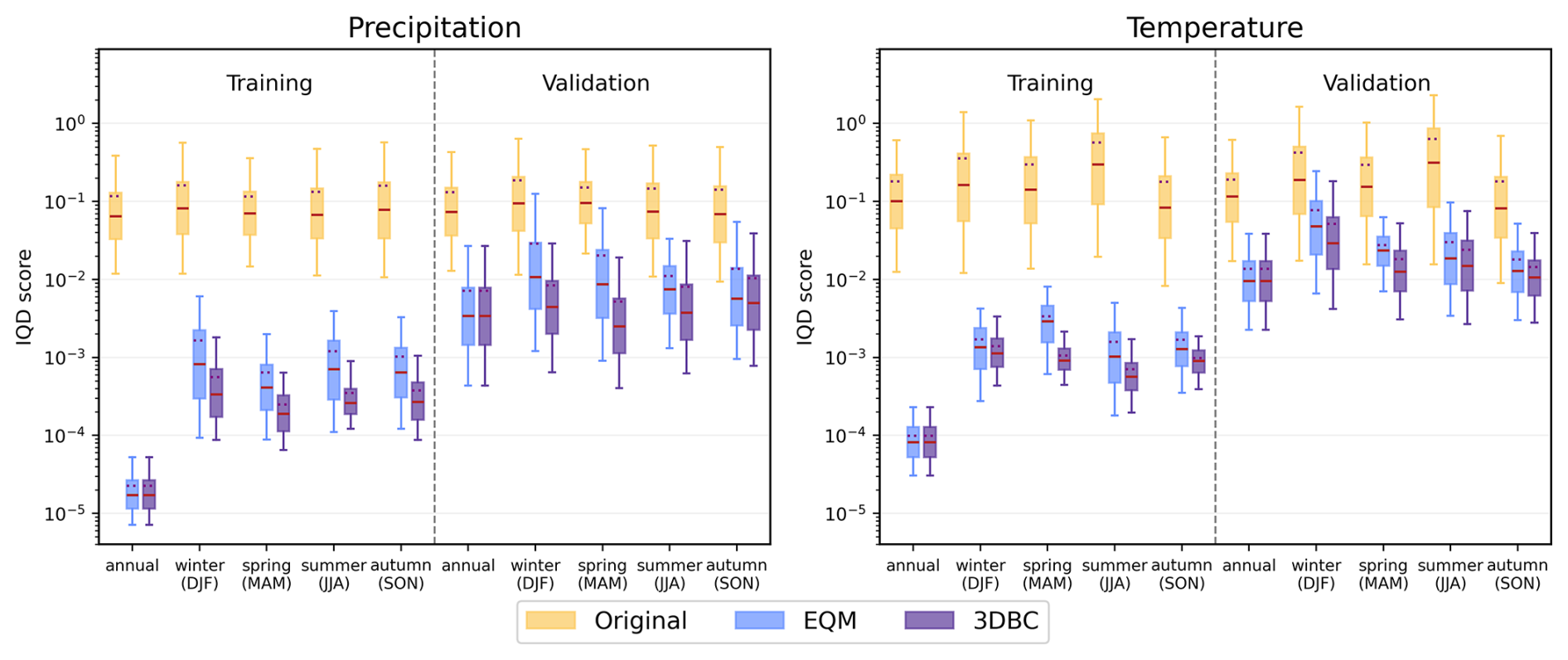
Figure 4 Integrated quadratic distance (IQD) scores for precipitation (left panel) and temperature (right panel) based on the CMIP5 model ensemble. Bias-adjusted results from EQM and 3DBC in addition to the original model outputs are compared with the reference datasets seNorge2018 v20.05 over the training (1985–2014) and validation (1960/70–1984) periods. The red line on the box indicates the median value whilst the dotted line represents the mean. The lower and upper boundaries of the box are the 25th and 75th percentiles. The lower and upper ends of the whiskers refer to the 5th and 95th percentiles.

IQD scores for precipitation and temperature are presented in Fig. 4. The results clearly demonstrate that both bias-adjustment approaches are far better at reproducing the full distributions of observed precipitation and temperature by several orders of magnitude than the original RCM outputs. As expected, the improvements are larger (smaller d_IQ) in the training period than the validation period. EQM and 3DBC have the same performance on annual results, but 3DBC generally performs better than EQM on seasonal results because 3DBC utilizes additional information about the intra-annual order of the observed time series in the post-processing. The only exceptions are the IQD scores from particular RCMs (CCLM4-8-17, REMO2015 and REMO2009), which show that EQM provides marginally better results than 3DBC in autumn (Fig. S1 in the Supplement). It might indicate that the observed ranks in autumn of the training and validation periods are quite different and that those models partly capture this change. Overall, 3DBC provides added value as compared to EQM when seasonal statistical properties are of importance.

Besides the seasonal statistics, 3DBC can simulate better spatial correlation structures between precipitation and temperature in the historical period than EQM, as it reorders the modelled ranks of precipitation and temperature based on observations while the univariate EQM method keeps the spatial rank correlation pattern from the RCM. Figure 5 shows an example of the spatial distribution of seasonal Spearman's rank correlation coefficient (ρ), calculated based on the bias-adjusted datasets from EQM and 3DBC and the reference datasets for training (1985–2014) and validation (1960–1984) periods for one RCM. In general, ρ are largest and positive in winter (warm days are wetter), followed by negative ρ in summer (warm days are dry, cold are wet). In spring and autumn, ρ is much smaller than in summer and winter, indicating a rather weak rank correlation between precipitation and temperature. The differences in the spatial correlation structure between these two methods are often most pronounced in winter and summer. EQM usually overestimates the positive rank correlations almost over the whole country in winter, whilst it underestimates negative dependencies in summer. And this spatial rank correlation pattern seems to be rather stable from one period to another. Aggregated results for each model combination are shown as boxplots (Fig. S2), and they confirm that 3DBC performs better in recovering the inter-variable spatial dependency structure for all RCMs.

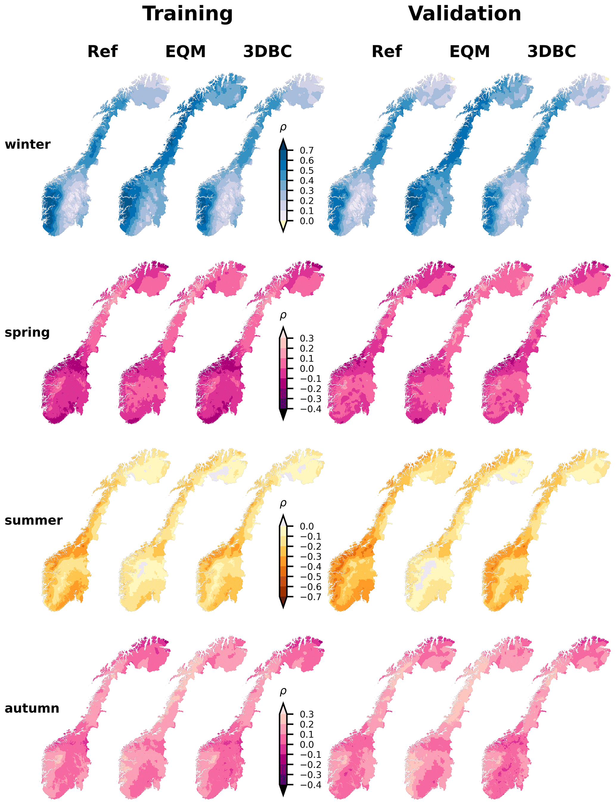
Figure 5 Spatial distribution of Spearman's rank correlation coefficient ρ of daily precipitation and temperature in winter (DJF), spring (MAM), summer (JJA) and autumn (SON) for the two bias-adjustment methods. For training (1985–2014) and validation (1960–1984) periods, the two bias-adjusted datasets, EQM and 3DBC are based on historical run from CMIP5-based mpi-r1i1p1-cclm and compared with reference datasets seNorge2018 v20.05.

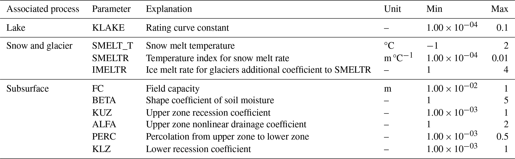
Table 2 List of calibration parameters. Note that the parameters associated with the snow and subsurface processes vary by land cover and soil type, respectively.

5.3.2 Climate change signal preservation

The two bias-adjustment methods can lead to different climate change signals in the future periods (e.g. 2071–2100) relative to the reference period (1991–2020). Figure 6 shows the annual and seasonal changes grouped in four elevation bands (< 500, [500, 1000 >, [1000,1500 >, > 1500), including 52 %, 32.7 %, 13.6 % and 1.7 % of the grid cells in Norway, respectively. The result aligns with other recent studies demonstrating that the change signals are elevation-dependent (Astagneau et al., 2025; Matiu et al., 2024). The two bias-adjustment methods provide identical annual climate change signals, since 3DBC uses the same bias-adjusted results from EQM before further post-processing. EQM generally preserves the seasonal climate change signals from the original RCMs in terms of both mean and median changes as well as the spread of changes for all elevation bands. However, by reshuffling the chronological order intra-annually, 3DBC modifies the seasonal change signals from the original RCMs, leading to larger increases in precipitation and temperature in winter and smaller increases in spring than the original RCM outputs. In summer and autumn, the climate change signals can be underestimated or overestimated by 3DBC depending on the variables and elevations.

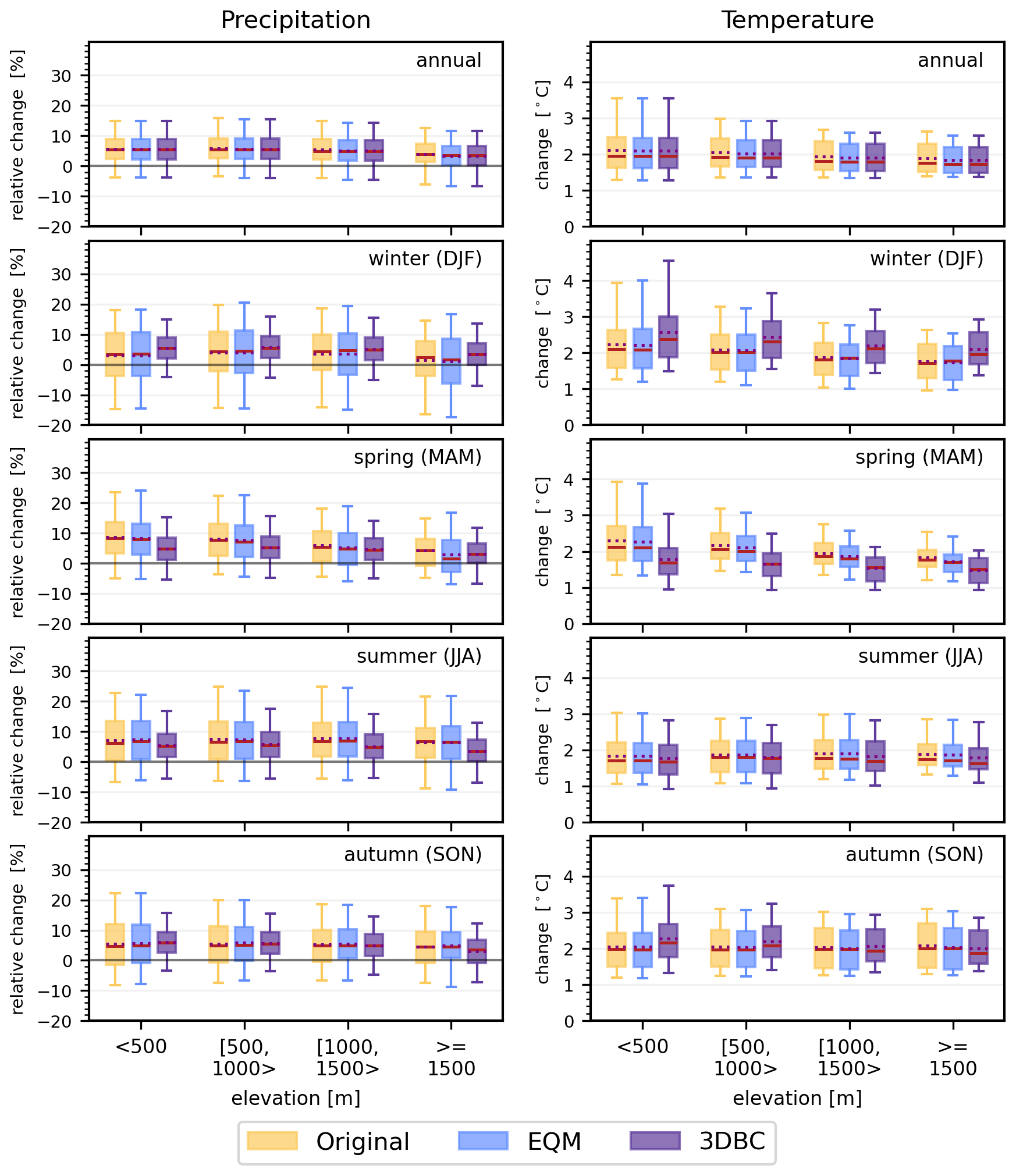
Figure 6 Projected annual and seasonal changes in precipitation (relative change in %, left column) and temperature (change in °C, right column) from 1991–2020 to 2071–2100 for RCP4.5 in terms of elevation. Results grouped in four elevation bands from two bias-adjustment procedures, EQM and 3DBC, are compared to the original RCM projections. The red line on the box indicates the median value whilst the dotted line represents the mean. The lower and upper boundaries of the box are the 25th and 75th percentiles. The lower and upper ends of the whiskers refer to the 5th and 95th percentiles.

6 Hydrological modelling

6.1 distHBV

distHBV is a spatially distributed version of the HBV precipitation-runoff model (Beldring et al., 2003) and is the major tool applied to assess hydrological responses to climate change in Norway. The model calculates the water balance for 1 km × 1 km grid cells at a daily time step covering the entire mainland surface area of Norway and upstream areas in Finland and Sweden contributing to streamflow in Norwegian catchments. Each grid cell includes one soil type and up to five land cover types. distHBV has components for accumulation, sub-grid scale distribution and ablation of snow, interception storage, sub-grid scale distribution of soil moisture storage, evapotranspiration, groundwater storage and runoff response, lake evaporation and glacier mass balance. The newly implemented Penman–Monteith method and the prescribed parameterizations are presented in Huang et al. (2019) and Erlandsen et al. (2021).

As for other conceptual hydrological models, calibration is necessary to adjust the distHBV parameters to improve the model performance of reproducing observed discharge, due to the absence of directly measured catchment characteristics, natural variability and the non-linearity of the processes involved. Since all parameters to calculate potential evaporation are prescribed in the Penman–Monteith equation, the calibration parameters are mainly associated with lake, subsurface, snow and glacier processes (Table 2). Different from the lumped version of HBV, the parameters associated with snow and subsurface processes in distHBV vary by land cover type (deciduous forest, coniferous forest and others) and soil-type (the five soil types based on the sediment map (Sect. 2.3) plus glacier bed), respectively. In total, there are 44 parameters for modelling mainland of Norway, including six snow parameters (two snow parameters times three land use classes), 36 soil parameters (six soil types times six subsurface parameters) and two parameters associated with lake and glacier processes. The parameters vary between grid cells due to different combinations of soil and land cover types within grid cells. Note that we didn't distinguish the snow parameters for all land cover types because it will increase equifinality risks due to too many calibration parameters and forest is one of the dominant land cover types in Norway (Huang et al., 2026). In addition, we didn't correct rainfall or snow as in other HBV applications, because it will lead to inconsistency between the climate and hydrological projections in terms of water balance.

The model was calibrated against discharges at 85 gauges (Fig. 1) from 2000 to 2007 using the parameter estimation routine PEST (Doherty and Skahill, 2006) and a multi-criteria calibration approach (Huang et al., 2019). The multi-criteria include the Nash and Sutcliffe efficiency (NSE) (Nash and Sutcliffe, 1970), the bias in water balance (BIAS) and the volume bias in the high-flow segment of the flow duration curve (ΔFHV, 0–0.02 flow exceedance probabilities) (Yilmaz et al., 2008). Since PEST minimizes the difference between the criteria results and their ideal values (1 for NSE and 0 for biases), the calibration objective function θ containing the three criteria at multiple gauges can be formulated as Eq. (7).

$$\begin{array}{}\text{(7)}& \begin{array}{rl}\mathit{\theta }=& W_{\text{NSE}}\times {\sum }_{i=\mathrm{1}}^n(\mathrm{1}-{\text{NSE}}_i{)}^{\mathrm{2}}+W_{\text{BIAS}}\\ & \times {\sum }_{i=\mathrm{1}}^n({\text{BIAS}}_i{)}^{\mathrm{2}}+W_{\mathrm{\Delta }\mathrm{FHV}}\times {\sum }_{i=\mathrm{1}}^n({\mathrm{\Delta }\mathrm{FHV}}_i{)}^{\mathrm{2}}\end{array}\end{array}$$

where W are weights for each criterion and n=85, the number of calibration catchments. W_NSE equals to 8 and W_BIAS and W_ΔFHV equal to 1 to achieve a good calibration performance.

Five PEST runs were carried out with different initial parameter values and only the parameter set giving the best model performance was selected for model validation. The model was validated against the discharge of the 85 calibration stations and additional 38 gauging stations from 2011 to 2020 to evaluate the temporal and spatial transferability of the model, respectively. The validation period (2011–2020) was selected because it is the warmest period for most catchments in the recent decades. Compared to the calibration period (2000–2007), the average increase in annual mean temperature of all 123 catchments is about 0.43 °C in 2011–2020. Hence, the validation results show the model performance under warmer conditions.

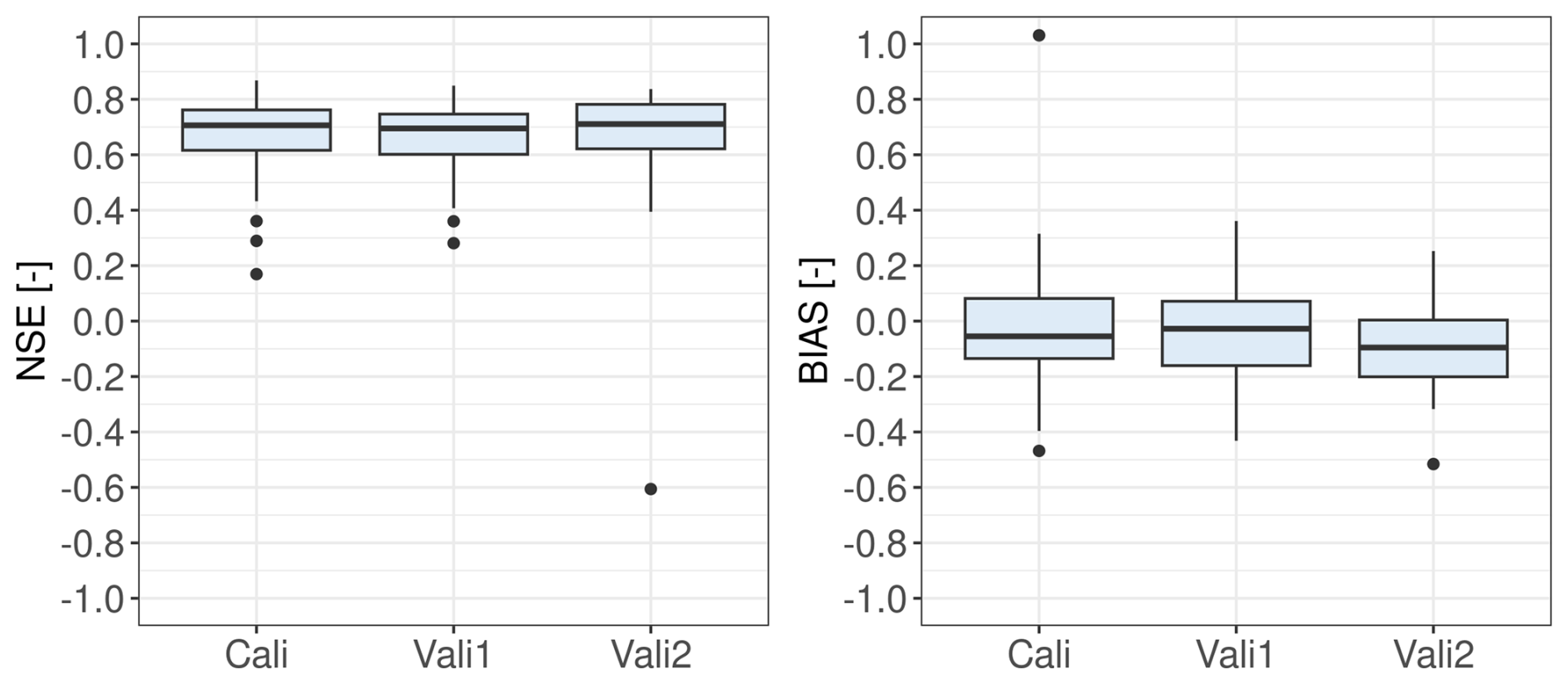
Figure 7 distHBV model performance in terms of NSE and BIAS for the 85 calibration catchments in the calibration period 2000–2007 (Cali), for the 85 calibration catchments in the validation period 2011–2020 (Vali1) and for the 38 validation catchments in the validation period 2011–2020 (Vali2).

Figure 7 shows the calibration and validation results in terms of NSE and BIAS. During the calibration period, about 50 % and 29 % of the catchments show good (NSE > 0.65 and |BIAS| < 0.1) and satisfactory (0.65 > NSE > 0.55 and 0.1 < |BIAS| < 0.15) results (Moriasi et al., 2007), respectively. The model generally underestimates discharge with the median bias of −5 %, mainly due to underestimation of precipitation in seNorge2018 v20.05 data. The model performs similarly in terms of NSE in the validation period for the 85 gauging stations, with the median NSE degraded by only 0.01. The median bias is reduced by 0.025 in the validation period than in the calibration period but there are more catchments with |BIAS| > 0.1. The model performance varies with time, partly due to parameter transferability problems under different climate conditions and partly due to the quality of seNorge2018 v20.05 dataset that also varies with time (Lussana et al., 2019; Lussana, 2020). The validation results for the additional 38 gauging stations show robust spatial transferability of the model, with good or satisfactory (NSE > 0.55 and |BIAS| < 0.15) model performance for about 58 % of the catchments. The model generally underestimates discharge with BIAS less than −0.1 for about half of the validation gauging stations. Such calibration and validation results are acceptable with consideration of the quality of the meteorological forcing data in such a mountainous region and simultaneous calibration for all catchments.

6.2 DEW

Distributed Element Water balance model (DEW) hydrological model (Beldring, 2008; Li et al., 2015) was used to simulate climate change impacts on glaciers for 12 given glacier regions in Norway. The smallest glaciers (< 1 km²) were omitted in the DEW model. This model differs from distHBV in the respect that it also calculates changes in glacier ice area, volume and surface elevation, and water balance. In addition, the model requires additional information as input, such as ice thickness and glacier area for grid cells with glaciers. However, DEW uses only daily mean temperature and precipitation as meteorological forcing data as it uses a temperature-based degree-day model to estimate potential evapotranspiration.

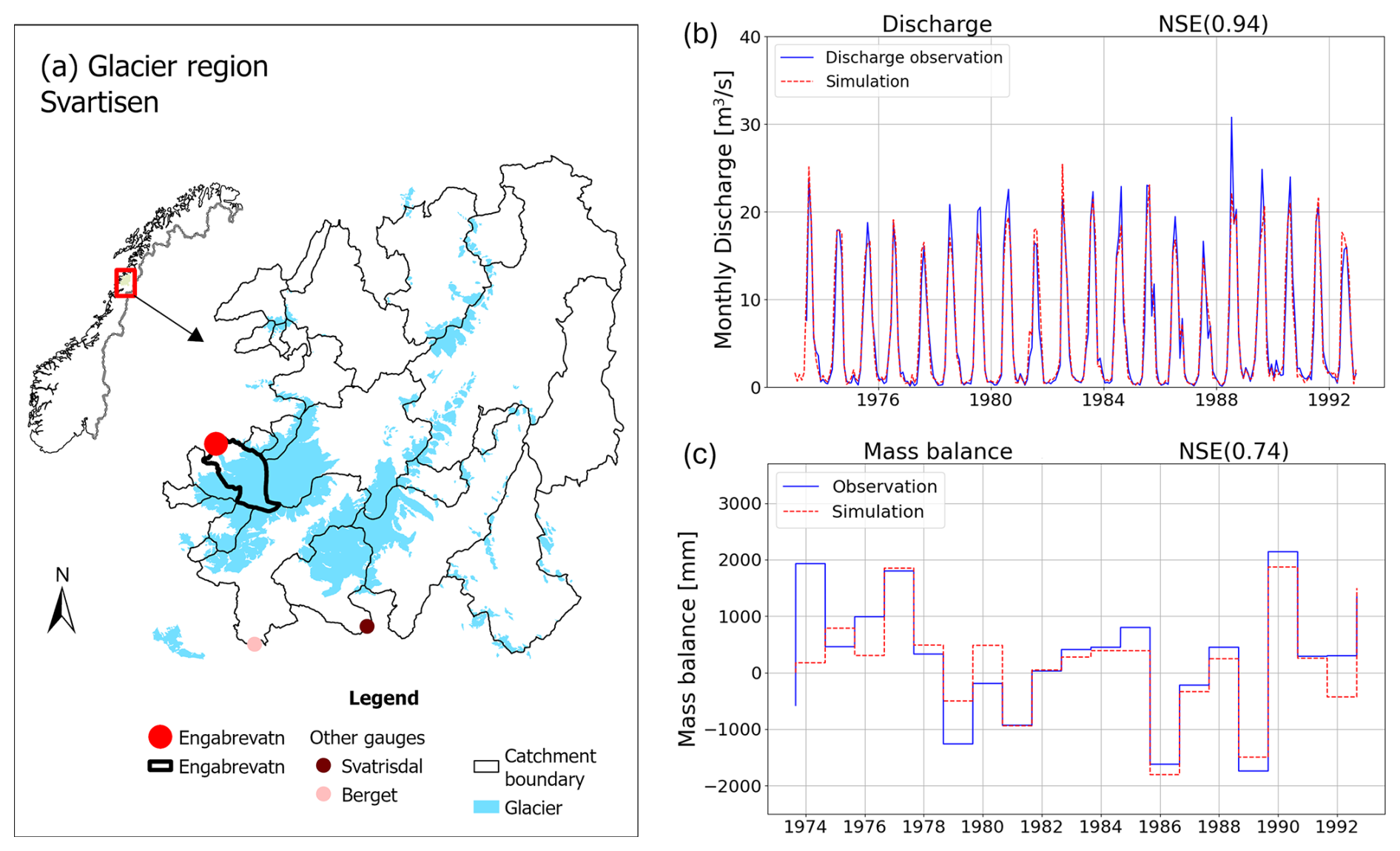
Figure 8 The glacier region Svartisen (a), observed and simulated discharge (b) and annual mass balance (c) for the catchment Engabrevatn.

Snow and glacier ice melt were calculated using a degree-day model, with different degree-day factors for snow and ice. DEW applies a simplified model called DeltaH (Huss et al., 2010) to describe the changes in glacier ice area, volume and surface elevation. The method simulates the impacts of ice movement that transports mass from the highest to the lowest areas of the glacier. Simulations without taking this redistribution of glacier ice into account will give incorrect estimates for both glacier changes and the water flow from the glacier. It is based on historically observed elevation changes of the glacier surface elevation and how these are distributed over the glacier area. The pattern of change is then used when simulating the development of glacier ice area, volume and surface elevation under climate scenarios by having the model redistribute mass over the glacier at the end of each mass balance year. Ice melt caused by negative mass balance results in diminishing of the glacier ablation area. Simulations with more advanced, physically based glacier models that simulate the flow of ice in the glaciers would probably be more realistic but are more demanding to run and require much more input data that are not available for most glacier areas in Norway.

DEW was calibrated using the same parameter estimation routine (PEST) as used for distHBV, but it was calibrated against observed daily streamflow and annual mass balance data for six out of the 12 glacier regions. Within each of the six regions, one optimal model parameter set was determined for all glaciers and catchments. This strategy was chosen to avoid discontinuities in model results between or along catchment boundaries and ice divides. Fixed periods were not used for calibration and validation as in the case of distHBV, because the availability of observed data varied both in time and space. It was a challenge to find both mass balance and streamflow time series of good quality at the same period, leading to limited time series available for model validation in some cases. During model calibration, mean NSE value is 0.75 for daily discharge of 19 gauging stations downstream of the glaciers, and 0.72 for annual mass balance for six glaciers. The mean NSE value for daily discharge during model validation is 0.74. For the remaining six glacier regions where there were no streamflow data available, model parameters were transferred from the nearest glacier region with calibrated parameters.

Figure 8a shows one of the 12 glacier regions, called Svartisen, as an example. For this region, DEW was setup for all catchments where glacier melt contributes to river discharge. Among these catchments, only three catchments (Engabrevatn, Svartisdal and Berget) have discharge observations in good quality and only Engabrevatn has the measured mass balance data. Based on the data availability of both discharge and mass balance data, DEW was calibrated against the discharge of the three catchments and glacier mass balance in Engabrevatn for the period 1974–1993. The calibrated parameters were then transferred to other catchments of this region for hydrological projections. Figure 8b and c compare the observed and simulated discharge and mass balance for Engabrevatn in the calibration period. It shows that the model can well reproduce both monthly discharge and annual glacier mass balance with NSE larger than 0.7.

6.3 Postprocessing of distHBV and DEW outputs

The final runoff projections for mainland Norway were produced by replacing distHBV outputs with the DEW ones. Note that DEW simulated the whole glacierized catchments but we only masked the glacierized grid cells in the historical period (e.g., the blue-color area within the catchments in Fig. 8a) for postprocessing. It is mainly because DEW uses a simpler potential evapotranspiration (PET) method and rougher landuse/soil classes for non-glacierized area than distHBV. The mask of the glacierized grid cells remained unchanged during the whole postprocessing procedure and the DEW outputs on the masked grid cells replaced the distHBV ones at each time step in both historical and future periods. Figure 9a and b shows the simulated runoff projections using DEW and distHBV for the glacier region Svartisen (Fig. 8a) on 31 August 2100 driven by the ecearth-r12i1p1-cclm climate projection. Without considering glacier retreat, distHBV projected high runoff (> 20 mm) for most grid cells where glaciers exist in the historical period while DEW projected much lower runoff for these grid cells than distHBV, confirming that distHBV overestimates runoff under warming conditions. After we replaced the distHBV results with the DEW ones, the final output is more reasonable for this region than the distHBV one (Fig. 9c). Note that there are still single grid cells with high runoff in the final product because of slightly different glacier maps used by DEW and distHBV. In addition, small glaciers outside the glacierized catchments (Fig. 8a) were not simulated by the DEW model and the results for these small glaciers cannot be corrected.

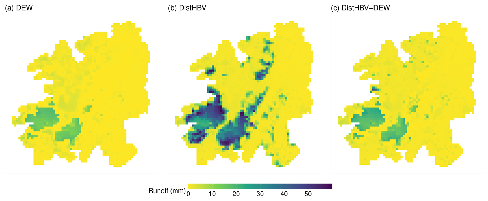
Figure 9 Simulated runoff on 31 August 2100 for the glacier region Svartisen by DEW (a), distHBV (b) and the combination of distHBV and DEW (c) driven by the ecearth-r12i1p1-cclm climate projection.

7 National climate projections

7.1 Ensemble means and ranges

There are 20 climate projections for mainland Norway at 1 km spatial resolution with daily time steps under the RCP4.5 scenario from the COR-BA-2025 dataset. Figure 10 shows 30-year running means of annual temperature and precipitation sums from 1971 to 2098 for Norway. There is a clear increase in temperatures visible in the mean and the whole ensemble. For precipitation, the ensemble mean is also increasing but the lower limit of the projection ensemble is showing a stable precipitation amount of about 1325 mm yr⁻¹. The observed historical values are mostly within the simulated precipitation and temperature ensembles but are located at the lower end of the ensemble before the year 2000 and at the upper end afterwards, indicating that the RCP4.5 ensemble underestimates recent temperature and precipitation trends in Norway. Note that all RCMs are bias-adjusted to match the observed values averaged over the training-period 1985–2014 and the spread in the ensemble equals zero for the middle of that period (year 2000). In addition, the ensemble spread is exactly the same for both EQM and 3DBC methods as 3DBC has the same change statistics as EQM on an annual basis.

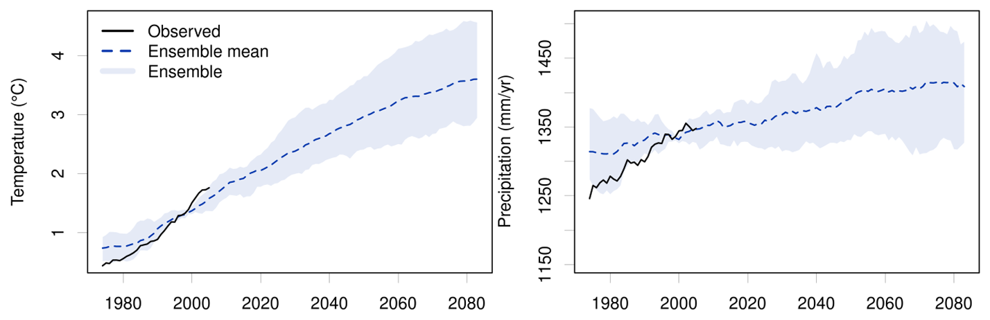
Figure 10 Simulated 30-year running means of temperature (left) and precipitation (right) from the COR-BA-2025 ensemble of 20 climate projections (10 GCM-RCM combinations × 2 bias-adjustment methods) for Norway under the RCP4.5 emission scenario.

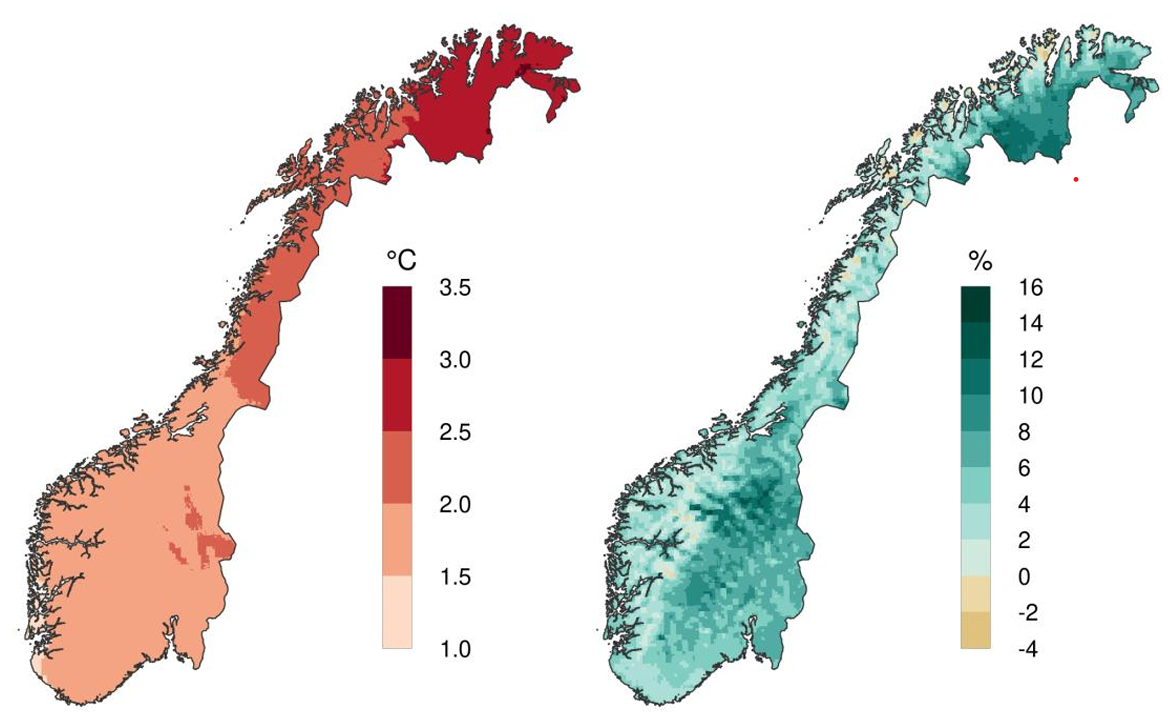
Figure 11 COR-BA-2025 ensemble mean changes in temperature (°C) (left) and relative changes in precipitation (%) (right) in the scenario period 2071–2100 relative to the reference period 1991–2020 under the RCP4.5 scenario for mainland Norway.

Looking at the spatial distribution of changes from the reference period 1991–2020 to the far future period 2071–2100 (Fig. 11), a generally larger increase in temperatures towards the North is apparent, with about 1 to 2 °C in the southern and 2 to 3 °C in the northern half of Norway. Precipitation is increasing as well with exceptions of some isolated areas along the coast and in the mountains. Generally, the precipitation increases are small and below +12 %.

7.2 Effects of two bias-adjustment methods

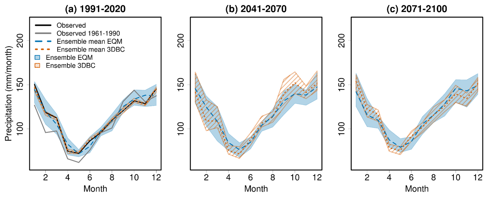
The effects of the two bias-adjustment methods on the preservation and altering of the seasonal climate change signals of the RCMs is shown in Fig. 6 and discussed in Sect. 5.3.2. Similarly, the two methods have different effects on the monthly climate change signal due to their design. While EQM is designed to preserve the monthly climate change signals, the 3DBC method is designed to provide spatial, temporal and inter-variable structures based on the reference data. However, as can be seen in Figs. 12 and 13, the shapes of the climatologies from EQM and 3DBC are similar and in agreement with the observed ones. As already seen for the seasonal changes (Fig. 6), precipitation and temperature changes in 3DBC are larger than in EQM in winter months (especially January and February) and smaller in spring and summer (April to June) for the far future period (2071–2100). For the near future (2041–2070), the difference in the changes from EQM and 3DBC are less systematic but 3DBC shows a pronounced increase in autumn precipitation which is absent in EQM (Fig. 13). This shift in the 3DBC results can be traced back to its implementation: the rank structure from the reference years 1961–1990 are used for the 2041–2070 period. Since the autumn precipitation in the period 1961–1990 has been large (Fig. 13a), this is imprinted on the mean annual cycle of the near future period. For the current climate (1991–2020), the 3DBC method results in climatologies that are similar for all models and thus a small ensemble-spread compared to the EQM data. This is especially true for precipitation (Fig. 13).

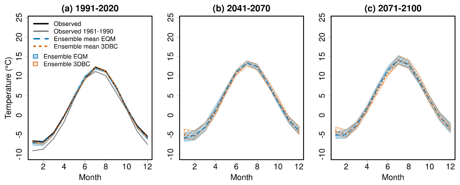
Figure 12 30-year mean monthly temperatures for Norway for different time periods using the EQM and 3DBC bias-adjusted climate projections under the RCP4.5 scenario. Black line: Observed temperature in 1991–2020. Grey line: Observed temperature in 1961–1990. Blue and orange lines: ensemble means of simulated temperature. Blue and orange striped areas: ensemble spread of 10 projections.

Figure 13 The same as Fig. 12 but for precipitation.

7.3 Uncertainty analysis

Besides the two different bias-adjustment methods, the various GCM-RCM combinations contribute to uncertainties in the climate projections. In this section, we analyse the contribution of these two uncertainty sources using the ANOVA method used by Vetter et al. (2017). Since each GCM is combined with different RCMs (see Sect. 4), we don't distinguish the GCMs and RCMs as different uncertainty sources here, but consider the GCM-RCM combinations as one uncertainty source. The two bias-adjustment methods are considered the second uncertainty source. The ANOVA method provides not only variations in the impact on temperature/precipitation from these two major sources, but also their interaction term. To avoid the bias caused by different sample sizes of the sources, the ANOVA was implemented for a number of subsamples, each of which includes two climate models and two bias correction methods, and then the obtained estimates of subsamples were averaged. For more explanation of the method and equations, please refer to Vetter et al. (2017).

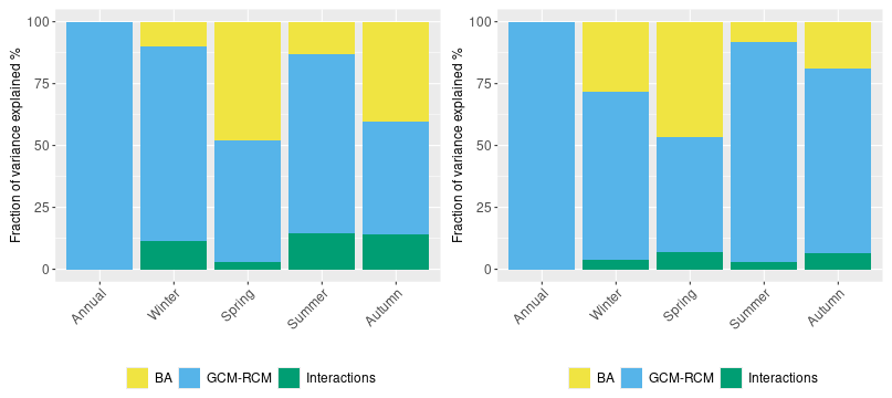
Figure 14 The fraction of variance in projected temperature changes explained by bias-adjustment methods (BA), GCM-RCM combinations and their interactions for the near-future period (2041–2070, left) and far-future period (2071–2100, right).

Figure 15 The same as Fig. 14 but for precipitation.

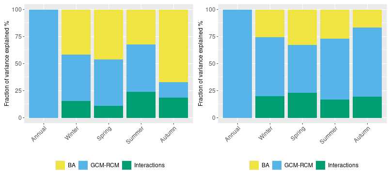
Since our implementation of 3DBC conserves the annual changes from EQM, the annual fraction of variance from the ANOVA analysis (Figs. 14 and 15) is solely dependent on the GCM-RCM combination. On a seasonal scale, the largest contribution to temperature uncertainties still comes from the GCM-RCM combinations. However, for spring and autumn the bias-adjustment contribution can be of similar size, especially in the near future projections. Interactions between the two uncertainty sources are generally small.

For precipitation, the contribution to the overall uncertainty from the bias-adjustment methods is larger than the contribution from the climate models for spring and autumn in the near future. Also for the other two seasons, the different contributions are of similar size for the near future. Interestingly, for the far future, the contribution from the climate models is clearly larger than the contribution from the bias-adjustment methods for all seasons. The interactions are larger than for temperature and can reach magnitudes similar to the single contributions. This is an effect of the two bias-adjustment methods resulting in seasonal change signals that differ more for precipitation than temperature, showing that results for temperature from a single bias-adjustment method are more robust than for precipitation. This is especially true for the near future.

Our findings bring new insights into uncertainty attribution for seasonal projections, because most studies on uncertainty attribution are mainly targeted at annual values rather than seasonal ones, e.g. Paz and Willems (2022) and Lafferty and Sriver (2023). There are only a few uncertainty analyses for seasonal changes, but they did not find larger uncertainty associated with bias-adjustment methods than the variability within the model ensemble (Tong et al., 2021; Zhang et al., 2024). Our results highlight that bias-adjustment methods can be an important uncertainty source for seasonal projections and their seasonal effects should be considered in future studies.

8 National hydrological projections

8.1 Ensemble means and ranges

There are 20 hydrological projections for mainland Norway at 1 km spatial resolution with daily time steps under the RCP4.5 scenario from the distHBV-COR-BA-2025 dataset. Figure 16 shows the projected annual sum/mean of these variables from 1971 to 2098 for mainland Norway. Both the ensemble means of runoff and evaporation have an increasing trend while the ensemble means of snow water equivalent and soil moisture tend to decrease towards the end of this century. The simulated runoff, evaporation, and soil moisture driven by the seNorge forcing data (black lines) are generally within the boundary of the 20 simulations in the historical period, and they have a good agreement with the ensemble mean around the year 2000. In addition, the spread of projections is reduced around the year 2000, as the bias-adjusted data matches the statistics of the observations better in the training period 1985–2014 than other periods. However, all snow water equivalent simulations are generally underestimated compared with the simulated snow water equivalent driven by the seNorge data, indicating that snow generation is not well reproduced. It is mainly due to inaccurate inter-variable, spatial and temporal dependence between the bias-adjusted atmospheric variables when only the EQM method is used (see Sect. 8.2).

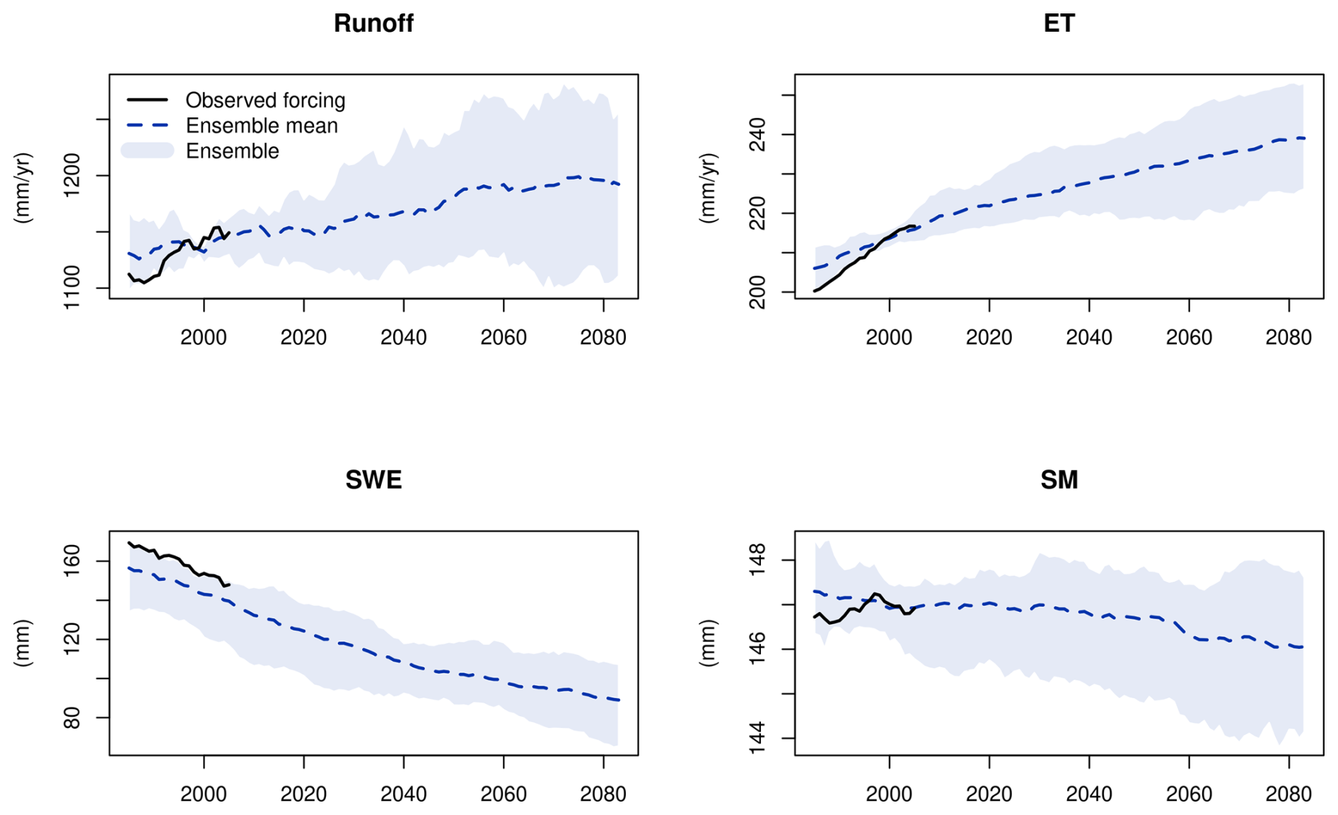
Figure 16 Simulated 30-year running means of annual runoff, evaporation (ET), mean snow water equivalent (SWE) and mean soil moisture (SM) driven by the ensemble of 20 climate projections (10 GCM-RCMs × 2 bias correction methods) under the RCP4.5 scenario. The black line is the simulated water components driven by the observed forcing data.

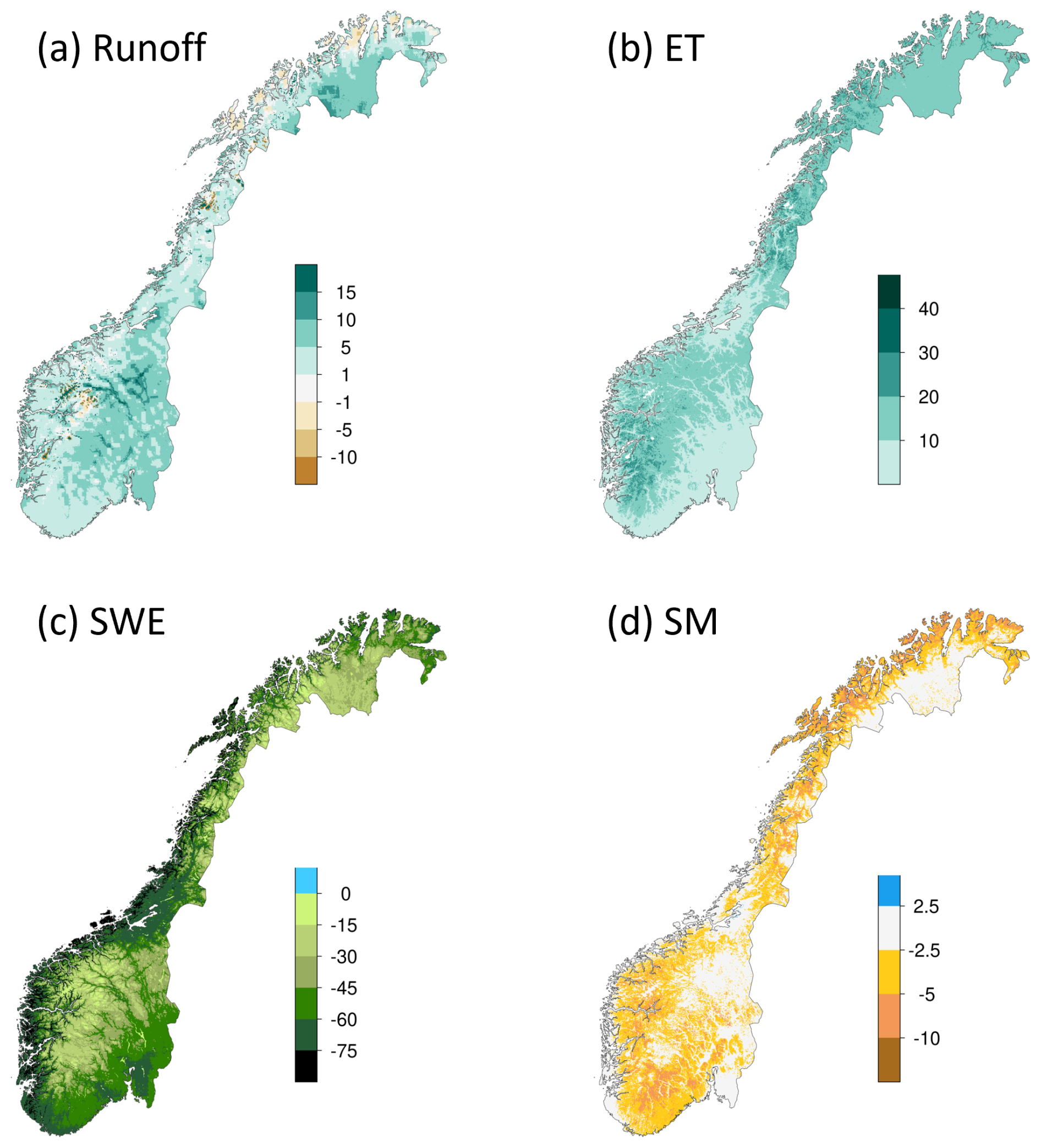
Figure 17 Ensemble mean changes (%) in annual runoff (a), evaporation (ET) (b), snow water equivalent (SWE) (c) and soil moisture (SM) (d) in the scenario period 2071–2100 relative to the reference period 1991–2020 under the RCP4.5 scenario for mainland Norway.

Figure 17 shows the spatial distribution of the ensemble mean changes in the last scenario period (2071–2100) relative to the reference period (1991–2020). In general, the increase in runoff is dominant in the whole country, except glacier retreat areas around the glaciers and the coastal areas in the northern part of Norway. The increases are minor (< 5 %) or moderate (5 %–10 %) in most parts of the country and strong increase in runoff (> 10 %) occurs mainly in the glacier areas, lakes and rivers as well as some northernmost areas. Due to the warmer and wetter climate in the future, evaporation is projected to increase in the whole country, especially in western and central Norway. In contrast, the annual mean snow water equivalent will decrease in the whole country in the far future, with a strong decrease (< −75 %) along the coast. Note that snow volumes along the coast of Southern Norway are small in today's climate. The absolute decrease in annual mean snow water equivalent is not stronger along the coast than mountainous areas. Soil moisture will decrease in most parts of the country due to the increase in evaporation and earlier snow melt, and moderate to strong decreases (< −5 %) are mainly found in some southern areas and the coastal regions in the north.

8.2 Effects of the two bias-adjustment methods

In this section, we provide a general overview of the effects of the bias-adjustment methods on hydrological projections. Figure 18 shows again the projected annual sum/mean of hydrological variables from 1971 to 2098 for mainland Norway, but separating the projections between the two bias-adjustment methods. The results show that the two bias-adjustment methods play a minor role on ensemble means as well as ensemble spread for runoff, evaporation and soil moisture, with the differences between the bias-adjustment methods less than 10 mm yr⁻¹ for runoff and evaporation and less than 1 mm for soil moisture. The ensemble mean of snow water equivalent using the 3DBC method has a better agreement with the results driven by observed forcing data than the ensemble mean using the EQM method, which always leads to underestimation of snow water equivalent in the historical period. In addition, the ensemble spread for snow water equivalent is narrower using 3DBC than EQM, especially before 2040, indicating lower uncertainty of projections using 3DBC. However, it is interesting to see that the snow water equivalent projections do not differ substantially after 2040 between the two bias-adjustment methods. Although the correlation structures and temporal sequences in the 3DBC data for this period are still similar to the observed ones in all models, different climate change signals in the RCMs lead to a larger overall spread in the driving variables, particularly temperature (Fig. 10). Thus, the resulting snow water equivalent projections using the 3DBC data inherit the general climate change signals and become similar to the EQM projections. The minor impact of bias-adjustment methods on annual values also leads to similar spatial distributions of the changes in runoff, evaporation and soil moisture, but considerable differences of changes in snow water equivalent are found along the coast and northmost Norway between the bias-adjustment methods (Fig. S3).

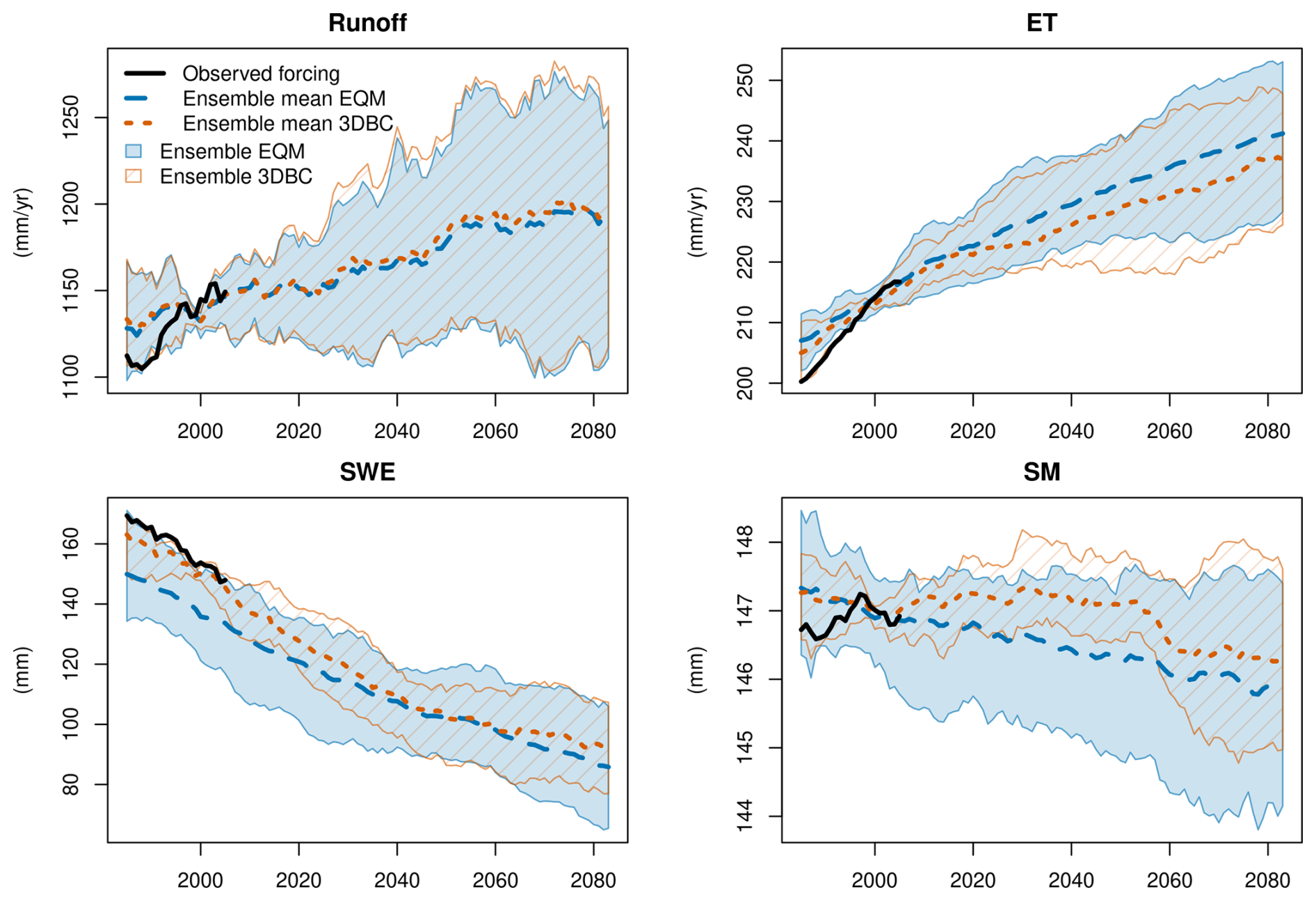
Figure 18 The same as Fig. 16 but the projections using different bias-adjustment methods are separated.

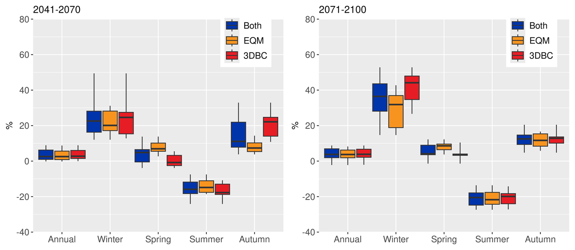
Figure 19 Relative changes in runoff for different seasons in the scenario periods 2041–2070 (left) and 2071–2100 (right) relative to the reference period 1991–2020 under the RCP4.5 scenario for mainland Norway.

Although the bias-adjustment methods affect the annual changes in runoff marginally, they lead to different seasonal runoff changes and their effects vary in scenario periods and seasons. Figure 19 shows the seasonal relative changes in runoff including all 20 projections, 10 projections using the EQM bias-adjustment method and 10 projections using the 3DBC method, respectively. In the near future, the largest difference in the ensemble median changes between the bias-adjustment methods is found in autumn (ca. 13 %), followed by the difference in spring (ca. 8 %), winter (ca. 5 %) and summer (ca. 3 %). The 3DBC method leads to higher runoff changes in winter and autumn, but lower runoff changes in spring and summer than the EQM method. As a result, the two methods lead to similar changes in annual changes. In the far future, the bias-adjustment methods mainly affect the runoff changes in winter and spring, resulting in a difference in median changes of 12 % in winter and 5 % in spring. There is almost no difference in median runoff changes between the methods in summer and autumn. These results indicate that the two bias-adjusted methods mainly affect the snow accumulation and melt processes, which occur in autumn, winter and spring in the near future and in winter and spring in the far future. In addition, 3DBC always leads to higher runoff in winter and lower runoff in spring than EQM in both scenario periods.

In order to illustrate the effects of the two bias-adjustment methods on snow processes, we compared the monthly snow water equivalent in the historical and scenario periods driven by different bias-adjusted projections as well as the ones driven by the observed forcing data (Fig. 20). In the historical period, the ensemble mean of monthly snow water equivalent driven by the 3DBC bias-adjusted projections agrees well with the simulated one driven by the observed forcing data. The EQM bias-adjusted simulations generally lead to underestimation of monthly snow water equivalent, especially in March and April, similar to the findings by Meyer et al. (2019). In addition, the historical snow simulations using the EQM method vary substantially between climate models, while all bias-adjusted climate projections using the 3DBC method lead to similar monthly SWE, indicating more robust snow projections in the historical period using the 3DBC method than the EQM method.

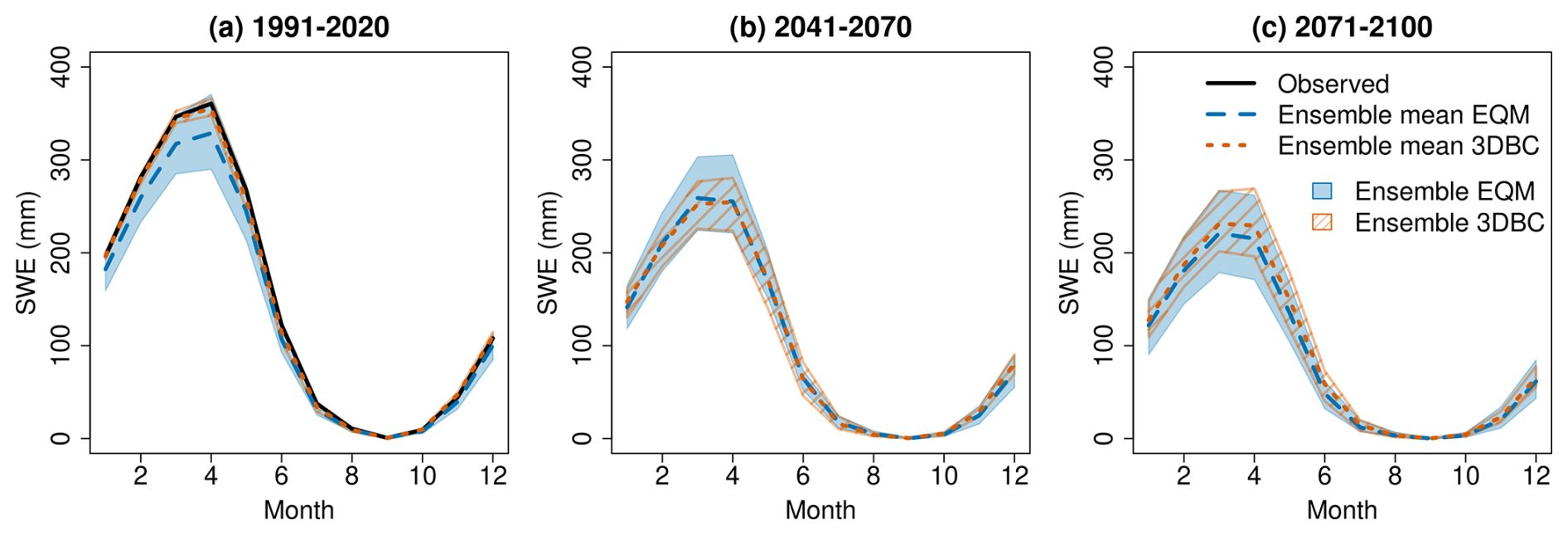
Figure 20 Simulated monthly snow water equivalent (SWE) for mainland Norway using the EQM and 3DBC bias-adjusted climate projections.

Figure 21 The same as Fig. 20 but for runoff.

The two bias-adjusted methods also affect the projected changes in snow water equivalent in the scenario periods, especially in the near future. The ensemble mean of monthly snow projections using the 3DBC methods show average decreases of about 4 and 55 mm month⁻¹ in the near and far future periods relative to the reference period, respectively, while the ensemble mean using the EQM method decreases by 33 and 50 mm month⁻¹ on average in the near and far future periods, respectively. It is due to higher snow water equivalent in the historical period and lower snow water equivalent in the near future using the 3DBC bias-adjusted projections than those using the EQM projections. However, the differences in snow water equivalent between the near and far-future periods are smaller using the 3DBC than the EQM method, leading to closer agreement on snow water equivalent changes in the far future between the two methods. The uncertainty bounds of snow projections using the 3DBC method are still smaller than the uncertainty bounds using the EQM method in both future periods, but the differences in uncertainty bounds between the two methods is less substantial than the ones in the historical period.

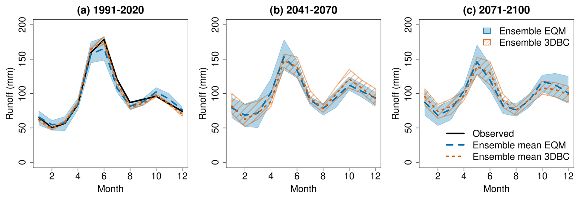
Partly due to different snow simulations, the monthly runoff projections also differ between the two bias-adjustment methods (Fig. 21). In the historical period, the simulated runoff using the 3DBC bias-adjusted climate simulations also agrees well with the simulated runoff using observed forcing data, while the simulations using the EQM bias-adjusted climate simulations underestimate runoff from June to July that is generated by snow melt, mainly due to less snow storage in winter and spring (Fig. 20). There is also an overestimate of runoff from October to November using the EQM bias-adjusted climate simulations, indicating that other hydrological processes besides snow are also affected by the inaccurate spatial and temporal correlations of climate variables. Similarly, the runoff simulations using the EQM bias-adjusted climate projections have larger uncertainty bounds than the ones using the 3DBC projections.

In the future periods, the runoff projections using the 3DBC method show larger increase and decrease in monthly changes relative to the historical period than using the EQM ones. In addition, the 3DBC bias-adjusted climate projections lead to higher runoff in autumn in the near-future than in the far-future while the EQM projections show contradicting changes. Different from the snow projection uncertainty, the runoff uncertainty using the 3DBC method is not always smaller than the one using the EQM method in all months. In addition, the large runoff uncertainty in the historical and future periods does not lead to large uncertainty of runoff changes. As shown in Fig. 19, the uncertainty bounds of runoff changes using the 3DBC method is not substantially larger than the uncertainty of changes using the EQM method.

8.3 Uncertainty analysis

Similar to temperature and precipitation, we assessed the contribution of the two bias-adjustment methods and GCM-RCM combinations to the uncertainty in the runoff projections. Figure 22 shows the fraction of variance from the ANOVA analysis for the GCM-RCM combinations, bias-adjustment methods and their interactions for the two future periods. For both periods, it is obvious that the climate model combinations contribute to the majority of the annual runoff change variance (> 90 %). However, the bias-adjustment methods play important roles in the seasonal runoff changes, especially in spring and autumn in the near future and in the winter and spring in the far future, explaining more than 50 % of the runoff change variance. For summer, the climate model combinations are always the major uncertainty source, explaining more than 50 % of the total runoff change variance. These results highlight the effects of bias-adjustment methods on seasonal runoff change projections.

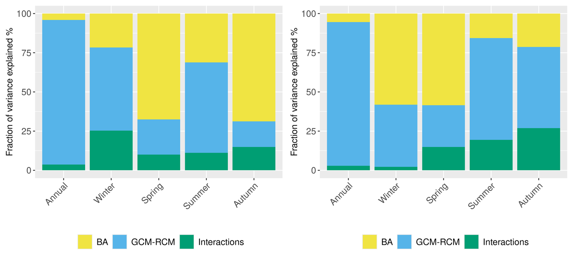
Figure 22 The fraction of variance in runoff change projections explained by bias-adjustment methods (BA), GCM-RCM combinations and their interactions for the near-future period (2041–2070) (left) and far-future period (2071–2100).

9 Discussion

9.1 Limitations of the methodology

In this study, we present the whole modelling chain that produces the updated national ensembles of climate and hydrological projections for the new Climate in Norway report CiN-2025 (Dyrrdal et al., 2025). This modelling chain includes selection of emission scenarios and climate models, downscaling and bias-adjustment methods and hydrological models. Although we have made a number of substantial improvements in each component of the modelling chain, there are still limitations and weaknesses in the methodology, which require further development for future climate impact assessments.

The first component in the modelling chain is to select appropriate emission scenarios and climate projections from a large ensemble of GCM and RCM outputs manageable throughout the complete chain. As a national climate assessment report following the sixth IPCC report, it would have been ideal to apply the most updated emission scenarios (i.e., the SSPs) and the corresponding climate projections. However, due to the long time needed to make the newest RCM results available within the CORDEX framework and the time limit of the national report, we had to apply the climate projections corresponding to the fifth IPCC report for the low- and median emission scenarios (RCP scenarios). Complements of the national climate projections for SSP emission scenarios are expected in the future to provide up-to-date knowledge on climate change impacts.

Since the EURO-CORDEX ensemble for the RCP scenarios is now much larger than for CiN-2015, the climate projections for CiN-2025 are more representative of the full range of climate changes ensembles. However, the restriction to ten models per scenario stemming from the complete modelling chain still partly limits the representativeness of the full possible outcome and model variability. In CiN-2025, this limitation is taken into account for temperature and precipitation using results from empirical-statistical downscaling (ESD) of the complete set of available GCMs. The ESD results are shown in the CiN-2025 report but not in this study as our focus is on the complete modelling chain. A detailed description of the ESD method used in CiN-2025 is given in Benestad et al. (2025).

RCMs are still subject to general limitations of model simplifications, such as internal parameterizations and spatial resolution. Further, some technical limitations remain in the RCM outputs, for example, some models provide outputs for 360 d per year, no leap year days or start in 1970 and end in 2098. This brings challenges for impact models and requires pre-processing before bias-adjustment. In addition, the historical period simulated by the RCMs does not cover the current standard normal period (1991–2020). This is a drawback since it is easier for the general public to compare the climate change signals with respect to the climate normal than other non-standard periods (e.g., 1976–2005). Although the use of the first few years from the scenario projections as reference period is not optimal, and the choice of the reference period can lead to different climate changes signals (Liersch et al., 2020), the use of the most recent standard normal period improves the public acceptance and understandability substantially, which is most important for the target users of a national report such as CiN-2025.

As the second component of the modelling chain, downscaling and bias-adjustment methods allow presenting projected climate and hydrological changes at a spatial resolution of 1 km × 1 km for the complex topography of Norway. Providing such high resolution data needs high computational costs and makes it challenging to test and apply a large number of bias-adjustment methods. Hence, we only selected EQM as the bias-adjustment method as it is robust for different climatological regimes and well established. The 3DBC method is further applied on the EQM bias-adjusted variables to improve the inter-variable, spatial and temporal dependencies. This multivariate bias-adjustment method indeed improves the hydrological projections, especially for snow simulations, and reduces the uncertainty range, especially in the reference period. However, the 3DBC method (Sect. 5.3) leads to different climate change signals compared to the original RCM signals on sub-annual scales because it imposes temporal dependency structures on the future projections similar to the ones from the reference datasets. This may be considered a weakness of the approach and more evaluation and development of multivariate bias-adjustment methods are required to further improve the existing methods. As discussed in François et al. (2020), the choice of method may differ from case to case, depending on which statistical properties from the RCMs need to be preserved or corrected. Based on our findings, users of the bias-adjusted data may select the appropriate dataset depending on their needs, or simply consider the two methods being equal, resulting in a broader ensemble.

In this study, RCM outputs have firstly been interpolated to the resolution of the observations (1 km) using the nearest-neighbour method and then bias-adjusted on that resolution. However, users should not overinterpret projected changes which are finer than the native RCM resolution (∼ 12.5 km) as the resolving power of the RCM sets the natural lower limit on which local-scale physical processes can be considered. Maraun (2013) has shown that the quantile mapping method cannot resolve this scale mismatch. This effect might be less important for temperature than precipitation as temperature usually has a much higher spatial coherence while precipitation is more subjected to small-scale variability. Although generally both the EQM and the 3DBC methods in our setup do not bring in climate change signals below the RCM resolution, some artifacts might be introduced which do not represent true local, small-scale climate changes.

Regarding hydrological models, both the potential evaporation module and glacier modelling have been improved compared to the model used in CiN-2015. The Penman–Monteith method improves evaporation estimates under climate scenarios by considering more climate variables and representing different land cover types (Huang et al., 2026), while the dynamic glacier modelling by DEW successfully avoids unrealistically high runoff from the glacier retreat areas under a warming climate. However, the simulations of distHBV may still suffer equifinality problems due to a large number of calibration parameters, which do not represent the physical characteristics of specific land use and soil types. In addition, we reclassify the soil types into five major groups in order to reduce the number of calibration parameters related to soil processes. This may lead to unreliable simulations for the areas where the soil condition is largely different from the major soil types. Therefore, both the calibration procedure and the spatial representation of soil physical characteristics are expected to improve in the future national applications.

Last but not least, vegetation types and characteristics are static in our hydrological modelling under climate change scenarios, but the changes in vegetation characteristics are expected under a warming climate. Huang et al. (2025a) assessed the effects of forest growth and forest management on water resources in six Norwegian catchments under the RCP2.6 and RCP4.5 emission scenarios. They found that forest growth would offset the increase in runoff in the catchments, where the deciduous forest is dominant. It implies that the runoff in the deciduous forest areas, especially in North Norway, may be overestimated in our present runoff projections. For the next generation CiN report, the land use and vegetation change scenarios should be included in the hydrological modelling if such scenarios are available.

9.2 Comparison of results between the old and new national reports

The improved modelling chain generated updated climate and hydrological projections for Norway, which resulted in slightly different climate change signals and climate impacts compared to the analysis in the old national report. Under the RCP4.5 scenario, the projections for the old and new national reports agree on the direction of change, but CiN-2025 projections display a smaller increase in annual temperature (ensemble mean of 2.0 °C) and precipitation (ensemble mean of 6 %) than the ensemble means in CiN-2015 (2.7 °C and 8 % increase in temperature and precipitation, respectively) at the end of the century. In addition, the ensemble spread in CiN-2025 is narrower than in CiN-2015, indicating more robust climate change signals. However, these differences are caused not only by the new selection of climate models, but also by the selection of the reference period. In CiN-2015, 1971–2000 was used as the reference period while in CiN-2025, it is 1991–2020. As temperature has already risen considerably in recent decades in Norway, annual mean temperature is higher in 1991–2020 than in 1971–2000, and the differences in temperature between the periods 2071–2100 and 1991–2020 are consequently more moderate than those between 2071–2100 and 1971–2000. In contrast, a larger increase in runoff is seen in CiN-2025 projections than in the previous one, mainly due to the improved evapotranspiration routine in the hydrological model (Huang et al., 2026).

Another major difference between the old and new national report is that CiN-2025 selected SSP3-7.0 as the high-emission scenario, which assumes lower emission than RCP8.5 used in CiN-2015. Under SSP3-7.0, the ensemble mean increases in annual mean temperature, precipitation and runoff are 3.4 °C, 11 % and 10 % in 2071–2100 relative to 1991–2020, respectively (Figs. S4, S5 and S16). These increases are also smaller than the ones in 2071–2100 relative to 1971–2000 under the RCP8.5 scenario, shown in the old national report. Hence, users who have made computations based on the CiN-2015 projections, should notice these differences and justify whether their computations should be updated or not.

9.3 The effects of bias-adjustment methods under the high-emission scenario SSP3-7.0

This paper comprehensively compared the two bias-adjustment methods applied to EURO-CORDEX RCP4.5 simulations and found that the two methods can lead to considerable differences in seasonal changes and snow simulations under the moderate-emission scenario. However, the impact of the bias-adjustment methods may not only vary between climate models and future periods but also between emission scenarios. Thus, results for the same comparison between the two bias-adjustment methods under SSP3-7.0 are included in the Supplement (Figs. S6–S19). Although the magnitudes of the projected changes between SSP3-7.0 and RCP4.5 differ, the general effects and differences between the two bias-adjustment methods are similar. One interesting aspect is a generally better agreement of the SSP3-7.0 ensemble mean temperature and precipitation with the observed values than in the RCP4.5 simulations during the reference period (Fig. S4).

For hydrological projections, 3DBC still provides better historical simulations than EQM under the SSP3-7.0 scenario, but the difference in future projections varies between the bias-adjustment methods and seasons. Considerable differences of ensemble mean changes in runoff are found in all seasons in the near future and in winter in the far future. The ensemble spreads of monthly projections for snow water equivalent and runoff are similar between 3DBC and EQM for almost all months, indicating that 3DBC does not help to reduce the projection uncertainty substantially under extremely warm conditions.

9.4 Application

Despite the limitations mentioned above, the COR-BA-2025 and distHBV-COR-BA-2025 datasets generated by the presented modelling chain provide the most updated, comprehensive and detailed hydrometeorological projections for mainland Norway. These national projections serve as the scientific basis for research on climate change impacts in Norway. The gridded hydrometeorological projections from CiN-2015 have already been used to derive new indices for specific application, e.g. snow-dependent tourism (Kuya et al., 2024; Mayer et al., 2023), reindeer husbandry (Hanssen-Bauer et al., 2022), frost decay exposure on building projects (Gaarder et al., 2024) and road maintenance (Nilsen et al., 2021). In addition to impact modellers, who represent an advanced user group, NCCS aims at providing tailored information for practical climate adaptation. Products derived from the national projections have also been widely used in local planning, mainly because government guidelines (Norwegian Government, 2024) required municipalities to take climate change into account in planning. Climate factsheets (Hisdal et al., 2021) provided the most relevant information to guide the climate adaptation work, and were pointed out as a core reference in government guidelines. See Nilsen et al. (2022) for an overview of the steps from climate model output to actionable climate information.

Besides the possibility to update existing applications that used the gridded dataset from CiN-2015, the new COR-BA-2025 and distHBV-COR-BA-2025 datasets provide additional variables, such as wind speed, pressure, evaporation, radiation and relative humidity, each bias-adjusted both with EQM and 3DBC. This improves the utility of the dataset for e.g., ecological modelling (see Pirk et al., 2023 for an example). It is expected that the new dataset will facilitate use in an even wider range of applications in the coming years, for climate change impacts on e.g., glaciers, drought, landslides and water availability. Further work will involve user groups such as municipal planners to co-create climate services based on the hydrometeorological projections presented.

In principle, we suggest using the full ensemble projections with both bias-adjustment methods to account for the uncertainty of the whole modelling chain. But in practice, users may want to select a subset of climate models and one bias-adjustment method to reduce the computational cost of further applications. As the users may be only interested in parts of Norway and the performance of climate models and bias-adjustment methods vary in space and time, we are not able to give a straightforward suggestion on the subset of climate models and bias-adjustment methods based on the national analysis. However, the methodology as well as the analysis in this paper provides examples of selecting models and bias-adjustment methods. In order to select a subset of climate models, the users can analyze the climate signals for their study area and periods as in Fig. 3 and then select the models based on the study purpose, e.g., studies aiming to assess the driest and warmest climate conditions or the wettest and coldest conditions in the near or far future. Based on the selected models, the users can further assess the seasonal trends for their study area and periods using both EQM and 3DBC projections as in Fig. 6. If the trends are comparable between the two bias-adjustment methods, the 3DBC adjusted projections can be preferred, especially when the study is focused on seasonal changes and snow processes. Otherwise, we strongly recommend to use the projections adjusted by EQM and 3DBC to account for the uncertainty of bias-adjustment methods.

Finally, we should note that the gridded datasets distHBV-COR-BA-2025 are not designed to use for flood indices, or climate change allowances for floods because distHBV was calibrated against many catchments simultaneously. Instead, the outputs from specific flood models should be used (Lawrence, 2020; Carr et al., 2023). The flood models include two lumped hydrological models and were calibrated against observed discharges for each catchment separately. Hence, the flood models produce more reliable estimates of high (and low) flow for specific catchments.

10 Conclusions

In this study, we present the whole modelling chain behind the production of updated national ensembles of climate and hydrological projections for the official “Climate in Norway” assessment report. We also provide insight into the hydrometeorological projections, which we termed COR-BA-2025 (standing for CORDEX-Bias Adjusted, updated in 2025) for climate projections and distHBV-COR-BA-2025 for hydrological projections, and analyse their uncertainties. The modelling chain (Fig. 2) includes the selection of GCM-RCM combinations for Norway from a large ensemble of EURO-CORDEX simulations, the application of two bias-adjustment methods and distributed hydrological modelling including a physically-based potential evaporation approach and a dynamic glacier model. Compared to the previous national assessment report, the new climate projections are considered more representative for Norway due to a larger ensemble of EURO-CORDEX simulations taken into account and a systematic analysis of the projections.

A multivariate bias-adjustment method has been applied for the first time over the whole of Norway for the complete atmospheric dataset consisting of nine variables. This new method leads to more consistent data in space, time and between variables, and to more robust hydrological simulations than the univariate empirical quantile mapping method (especially for snow and in the reference period), but it does not preserve climate change signals on a sub-annual scale. However, the uncertainty ranges of runoff change projections are not significantly different between the two bias-adjustment methods, especially at the annual scale. An uncertainty analysis shows that the climate projections are the major source of uncertainty for annual runoff change, while the selection of the bias-adjustment method plays an important role on seasonal changes.

Despite the advancement in the presented methodologies and modelling chain, there is still room for further improvement in future climate impact assessment studies. Currently we foresee that additional emission scenarios and GCM-RCM combinations from the EURO-CORDEX initiative will be evaluated and the bias-adjustment methods will be further developed to overcome the current limitations. In addition, the calibration procedure and the calibration parameters in the hydrological modelling will be further improved using advanced machine learning techniques. If possible, the land use and vegetation changes scenarios should also be considered in hydrological modelling.

The methodological description provided here serves as core knowledge for any further application of the gridded products, which are expected to be used in a wide range of climate impact assessments and development of climate adaptation strategies in Norway. We have thrived to meet the FAIR principles (Wilkinson et al., 2016) for data management. Thus, the complete COR-BA-2025 and distHBV-COR-BA-2025 datasets (Wong et al., 2025) are findable and accessible through the Arctic Data Centre (adc.met.no) at https://doi.org/10.21343/0k90-6w67. The data is stored in NetCDF format following the attribute convention for data discovery (ACDD version 1-3, https://wiki.esipfed.org/Attribute_Convention_for_Data_Discovery_1-3, last access: 28 April 2026) and the climate and forecast metadata conventions (CF version 1.10, Eaton et al., 2022). The code and data are reusable, being open source with non-restrictive licenses.