A hybrid framework for the spin-up and initialization of distributed coupled ecohydrological-biogeochemical models

Accurate initialization is a critical step in fully distributed ecohydrological and soil biogeochemical modeling applications, yet is often hindered by the computational cost of achieving steady-state conditions across large spatial domains. This study presents a novel initialization framework that combines a flux-tracking 1D spin-up with a random forest (RF) algorithm to efficiently generate spatially heterogeneous and topography-informed initial conditions accounting for lateral fluxes of water, carbon, and nutrients. The framework first performs a limited number of 1D simulations to obtain steady-state conditions in a subset of representative cells, then uses RF to extrapolate these results across the catchment. Applied to T&C-BG-2D, a fully coupled distributed ecohydrological-soil biogeochemical model, the scheme reconstructs over 90 % of the spatial variability in soil carbon and nutrient patterns in terms of probability distribution similarity while reducing computational demands by up to 90 % compared to a fully distributed spin-up procedure. A sensitivity analysis across multiple simulation scenarios reveals that the number of tracked cells required, varying from 20 % to 40 % of total domain grid cells, depends on the catchment's spatial complexity and the environmental covariates embedded in the RF predictors. The framework developed here can be applied to other spatially distributed models that explicitly account for lateral transfer fluxes, enabling large-scale distributed ecohydrological-biogeochemical model initialization under constrained computational budgets.

1 Introduction

Process-based ecohydrological and biogeochemical models have become widely used tools to study the cycling of water, carbon, and nutrients, and to predict ecosystem responses to anthropogenic and climatic changes. However, initialization remains a critical challenge in ecohydrological modeling (Thornton and Rosenbloom, 2005; Hashimoto et al., 2011), as initial conditions strongly influence model outputs and can substantially reduce the model’s ability to predict short-term responses to climatic variability (e.g., Senarath et al., 2000). This issue becomes even more critical for models including soil biogeochemical components and aiming to simulate the coupled dynamics of water, vegetation, and soil biogeochemistry (Thornton and Rosenbloom, 2005; Fatichi et al., 2019; Lian et al., 2025b). A common practice to specify initial conditions for model simulations is to run a model for a chosen time period until equilibrium (dynamic or steady state) is reached (Thornton and Rosenbloom, 2005; Seck et al., 2015). The duration of this spin-up process largely depends on the chosen initial state, the model parameters, and the prescribed forcings (Thornton et al., 2002; Thornton and Rosenbloom, 2005; Shi et al., 2013). For hydrological models, this stabilization period typically spans days to several years, depending on the variable of interest (e.g., Noto et al., 2008; Seck et al., 2015; Kim et al., 2018; Baroni et al., 2019). In contrast, soil biogeochemical models often require much longer spin-up periods, sometimes up to thousands of years (Randerson et al., 2009; Qu et al., 2018; Sun et al., 2021), to stabilize soil carbon and nutrient pools and avoid unrealistic behavior caused by disequilibrium in biogeochemical fluxes (Thornton and Rosenbloom, 2005; Lugato et al., 2014; Ammann et al., 2009; Nemo et al., 2017).

To reduce the computational burden of long spin-up periods, various strategies have been proposed for plot- or ecosystem-scale models. Analytical solutions under simplified forcing conditions can be used for some terrestrial biosphere models (Zhan et al., 2003; Xia et al., 2012; Qu et al., 2018; Schwarz et al., 2024). Thornton and Rosenbloom (2005) introduced several acceleration techniques in the Biome-BGC model, including accelerated decomposition, nitrogen addition, and multivariate minimization. These approaches reduced spin-up time by up to 75 %. Hashimoto et al. (2011) developed a “slow-relaxation scaling” method to gradually adjust soil carbon and nitrogen pools, improving the stability and realism of spin-up in the CENTURY model. Other approaches include performing spin-up of specific sub-modules only (Krinner et al., 2005), or integrating spin-up procedures with data assimilation techniques to reduce computational demands across multiple sites (Ng et al., 2014). Table S1 in the Supplement presents a non-exhaustive list of spin-up methods and their applications across coupled ecohydrological-soil biogeochemical models applied at plot and ecosystem scales.

Model initialization is even more challenging in spatially distributed coupled ecohydrological-biogeochemical models (e.g., Tague and Band, 2004; Shi et al., 2018; Lian et al., 2025b), which require information on distinct soil carbon and nutrient pools, whose spatial distributions are largely modulated by a combination of climatic, pedogenic, topographic, and biological landscape attributes (Li et al., 2020; Lian et al., 2025b; Parvizi and Fatehi, 2025). Due to the scarcity of spatially explicit data on soil biogeochemical pools, most models apply uniform or averaged initial conditions, followed by a spin-up period (typically a few years) to stabilize the system (e.g., Tague and Band, 2004; Zhang et al., 2018; Qiu et al., 2023). In the most extreme case, Christensen et al. (2008) applied a spatially distributed spin-up of more than 2500 years to reach steady state of soil carbon and nitrogen pools. However, prolonged spin-up periods can become computationally prohibitive when applied to thousands of grid cells. Moreover, existing initialization techniques, often designed for plot-scale models or coarser spatial resolutions, are insufficient for spatially distributed systems, as they neglect the effects of lateral transfers of water, carbon, and nutrients among computational cells in evaluating the long-term steady state.

Recent advances in artificial intelligence and machine learning (ML) have provided new opportunities for environmental modeling, including applications in hydrology, ecology, and soil science (e.g., Peters et al., 2007; Mahdavi et al., 2018; Tyralis et al., 2019; Carranza et al., 2021; Gupta et al., 2021; Sun et al., 2023; Pawusch et al., 2025). In spatially distributed models with limited data availability, ML methods, such as random forest (RF) approaches, offer a practical approach to estimate initial conditions. RF approaches have been successfully applied in hydrology and soil science (e.g., for landcover classification, soil moisture estimation, and mapping of soil hydraulic properties). These successes highlight their ability to extrapolate spatial distributions of soil carbon and nutrient pools using environmental covariates, based on a limited number of locations with known steady-state conditions (Martin et al., 2014; Parvizi and Fatehi, 2025; Zeraatpisheh et al., 2022). In this context, if steady-state conditions are known for a subset of grid cells, RF can be used to infer the spatial distribution of biogeochemical pools across the entire catchment. However, a workflow for the effective use of RF approaches to initialize coupled, spatially-distributed ecohydrological-biogeochemical models is currently not available.

The goal of this study is to develop a generalizable and computationally efficient methodology to initialize spatially distributed ecohydrological–biogeochemical models in complex catchments. Achieving this goal requires addressing three main challenges: (i) the high computational demand of fully coupled spin-up procedures for soil carbon and nutrient pools, (ii) the even greater computational costs of applying such spin-up in distributed 2D simulations, and (iii) the need for a strategy that can be generalized across catchments with different levels of topographic complexity and soil and vegetation variability. To overcome these limitations, we propose a novel initialization scheme that combines a plot-scale flux-tracking spin-up with a RF algorithm. The proposed spin-up procedure captures lateral transfers of water, carbon, and nutrients, while the RF model uses well-established key controlling factors (i.e., topography, vegetation, and soil information) to reconstruct spatial patterns of soil carbon and nutrient pools. We implement this framework in the recently developed fully distributed coupled ecohydrological-soil biogeochemical model T&C-BG-2D (Lian et al., 2025b) and test the following hypotheses:

• (H1) Spatially explicit spin-up is required to capture spatial variability in soil carbon and nutrient pools at the catchment scale, where grid-cell hydrological connectivity and topography-driven heterogeneity in water and energy states concurrently act to shape soil biogeochemical spatial patterns;

• (H2) Performing spin-up with lateral transport only at a subset of representative locations and extrapolating the results statistically with a RF model provides sufficient accuracy;

• (H3) The number of representative locations required depends on the overall heterogeneity of the catchment as well as on the specific predictors included in the RF model (e.g., additional soil or vegetation attributes);

• (H4) Uncoupled spin-up simulations (soil biogeochemistry dynamics with constant vegetation fluxes) provide adequate steady-state conditions for the model initialization.

To our knowledge, this is the first study to address initialization in a catchment-scale, fully distributed coupled ecohydrological-soil biogeochemical model, which mechanistically simulates coupled water, vegetation, and soil biogeochemical dynamics and explicitly accounts for water and solute lateral transport as well as topography-controlled variations in microclimatic conditions. The proposed approach provides a flexible and computationally efficient solution to spatial initialization and can be readily adopted in other modeling frameworks.

2 Materials and methods

2.1 T&C-BG-2D model and study area

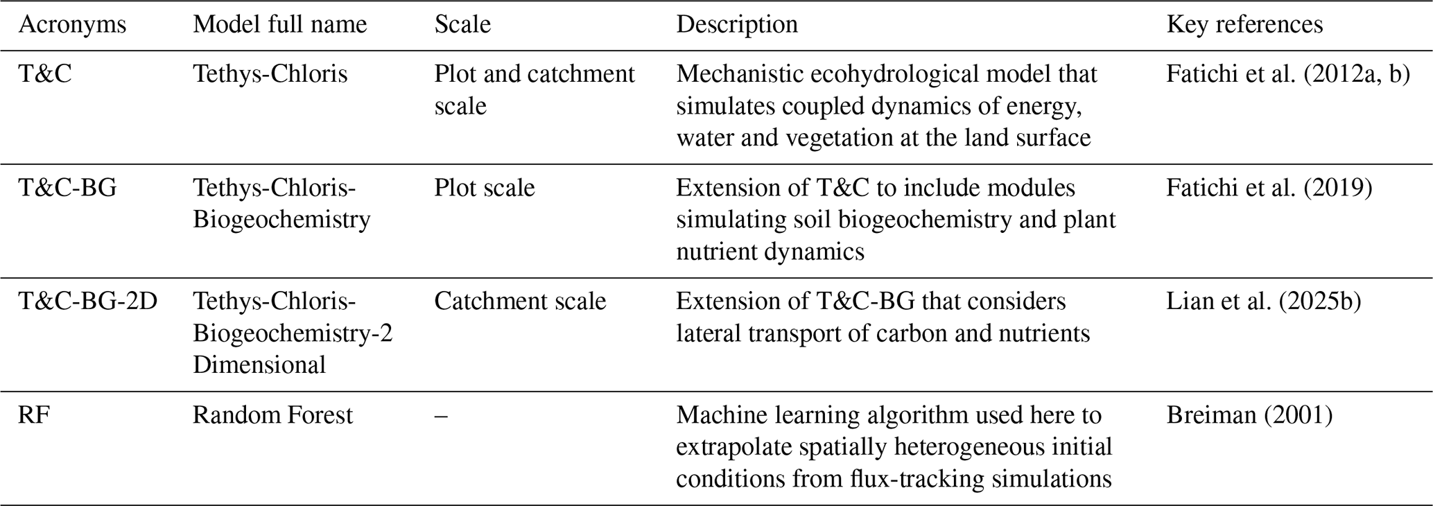
In this work, we use the recently developed coupled ecohydrological-soil biogeochemical model, T&C-BG-2D (Lian et al., 2025b), to evaluate the effect of different initialization schemes on the spatial distribution of soil carbon and nutrient pools. The original T&C model (Fatichi et al., 2012a, b) simulates coupled water, energy, and carbon cycles at the land surface. It includes modules for soil moisture dynamics and vegetation processes such as plant phenology, carbon allocation, and tissue turnover (Fatichi et al., 2012a, b, 2016). The hydrological component simulates precipitation interception, transpiration, evaporation, infiltration, and snow/ice hydrology. Soil water movement is represented using a quasi-3D Richards equation, while surface water flow uses a kinematic wave approach (Paschalis et al., 2022). A soil biogeochemistry component, T&C-BG (Fatichi et al., 2019), was integrated into the T&C model to simulate soil carbon and nutrient dynamics, including nitrogen (N), phosphorus (P), and potassium (K). Vegetation growth is regulated by the availability of these nutrients, as plant tissue formation depends on flexible target stoichiometric constraints between carbon and nutrients, and nutrient limitation can constrain biomass production. The biogeochemistry module partitions plant litter into pools based on decomposability, and represents soil organic carbon (SOC) in three functional forms (mineral-associated, particulate, and dissolved). Soil organic nitrogen (SON) dynamics are tightly coupled to carbon through stoichiometric C : N ratios. The model simulates the temporal dynamics of SON, dissolved organic nitrogen (DON), and nitrogen stored in microbial and macrofauna biomass. It also explicitly tracks inorganic nitrogen pools – ammonium (NH${}_{\mathrm{4}}^{+}$) and nitrate (NO${}_{\mathrm{3}}^{-}$) – whose dynamics are regulated by mineralization, immobilization, biological uptake, leaching, volatilization, nitrification, and denitrification. A comprehensive description of T&C-BG is available in Fatichi et al. (2019) and Botter et al. (2021). Recently, Lian et al. (2025b) extended T&C-BG to a distributed framework (T&C-BG-2D) by explicitly accounting for the lateral transport of seven mobile carbon and nutrient pools, including DOC, NH${}_{\mathrm{4}}^{+}$, NO${}_{\mathrm{3}}^{-}$, dissolved inorganic phosphorus (DIP), dissolved potassium ions (K⁺), DON, and dissolved organic phosphorus (DOP), considered as passive tracers transported following the water flow. Tracers are assumed to be well-mixed in each storage compartment after vertical/lateral transport. At each hourly time step, the model updates soil carbon and nutrient pools in each grid cell by accounting for laterally transported solutes, which in turn regulate local vegetation dynamics. This enables the simulation of coupled ecohydrological-soil biogeochemical dynamics with the explicit consideration of the role of topographic features and lateral transport in shaping spatio-temporal carbon and nutrient patterns across a landscape. For clarity, Table 1 summarizes the different models referred to in this study. The proposed hybrid initialization technique is implemented in the coupled ecohydrological–biogeochemical T&C-BG-2D model.

Fatichi et al. (2012a, b)Fatichi et al. (2019)Lian et al. (2025b)Breiman (2001)

Table 1 Acronyms, full names, spatial scales, and brief description with key references of the models mentioned in this study. Note that the proposed hybrid initialization technique is for the fully distributed coupled ecohydrological-soil biogeochemical T&C-BG-2D model.

The domain used to test and showcase the spin-up procedure in this study is the Erlenbach catchment (Fig. 1a), a 0.76 km² basin in the central Swiss Pre-Alps (Stähli et al., 2021) where T&C-BG-2D has already been applied (Lian et al., 2025b). We considered a spatial square grid resolution of 20 m. Based on a previous application of T&C-BG-2D in this catchment (Lian et al., 2025b), we used meteorological data to force the model covering a 9-year period (1 October 2011 to 30 September 2020). During this time, the catchment received an average annual precipitation of 2200 mm, with a mean air temperature of 6.5 °C (Lian et al., 2025b). The spatial distribution of soil texture (here mostly loam and clay loam) was retrieved from Gupta et al. (2024), and vegetation cover was obtained from Pazúr et al. (2021). As only one meteorological station (Erlenhöhe) is available in Erlenbach, constant lapse rate values typical of the region were assumed. For example, we considered a constant thermal lapse rate equal to −0.0045 °C m⁻¹ (Nigrelli et al., 2018; Lian et al., 2025b). The Erlenbach catchment is a suitable study area to showcase the spin-up and initialization procedure proposed here since model parameters have already been calibrated and the area is relatively small (thus reducing the computational costs) but still with a highly pronounced topography. Specific model settings and parameters for the simulations here can be found in Lian et al. (2025b).

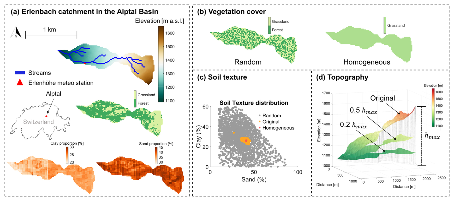
Figure 1 The Erlenbach catchment (a) and the modified catchment configurations (b–d) used to test the proposed initialization procedure. (a) Original catchment characteristics showing topography, stream network, vegetation cover, and sand and clay fractions. (b) Alternative vegetation scenarios: randomized grassland and forest cover (left), and homogeneous grassland (right). (c) Soil texture scenarios, represented in a sand–clay triangle: original soil texture (orange), randomized soil texture distribution (gray), and homogeneous soil texture (red). (d) Topographic scenarios generated by scaling the original digital elevation model by factors of 0.5 and 0.2.

2.2 Initialization procedure

The core strategy for the initialization framework proposed here involves two main steps: (1) performing a plot-scale spin-up in a limited number of selected cells while explicitly accounting for lateral fluxes of water, carbon, and nutrients, and (2) using a RF model to extrapolate the resulting steady-state pools across the entire model domain. While the RF is not used here to predict an independent external reference state, it enables spatial generalization from the sampled tracked cells to the remaining ones across the catchment. A primitive version of this procedure was successfully applied in Lian et al. (2025b). However, no formal workflow was developed, and neither large-scale benchmarking nor a systematic sensitivity assessment of the method was conducted. In this study, we formalize the framework, evaluate its performance across multiple scenarios, and test its generality to enable seamless application in other models and study areas.

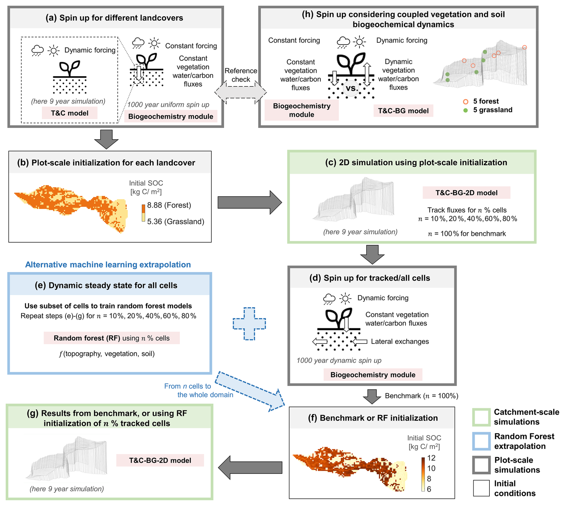
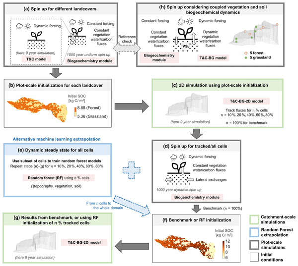
Figure 2 Workflow of the model initialization procedure. (a) For each soil–vegetation combination, the T&C model is used to obtain averaged water and plant fluxes, which are used in a 1D spin-up via the T&C-BG biogeochemistry module using long-term average meteorological inputs. The resulting steady-state pools are then assigned to all cells with the same soil–vegetation combination (b). (c) A 2D simulation (T&C-BG-2D) is run with these initial conditions, tracking fluxes for all cells (benchmark) or for a given percentage n of all grid cells. (d) For these cells, the T&C-BG biogeochemistry module 1D spin-up with dynamic meteorology and imposed lateral fluxes is run to achieve a dynamic steady state in all tracked cells. (e) A random forest (RF) model is trained on results from different percentages (n) of the subset of these cells using topographic, soil, and vegetation attributes as predictors to reconstruct the initial conditions for the entire catchment domain (f), which are then used to initialize the final simulations (g). For each simulation scenario, steps (e) to (g) are repeated for different percentages of tracked cells n to investigate the optimal number of cells for the RF algorithm. (h) Additional plot-scale simulations are performed for 10 representative cells (5 forest, 5 grassland) to obtain a reference steady state using the fully coupled T&C-BG model (i.e., also considering dynamic vegetation fluxes), which is compared to the initial states generated in step (a). The solid arrows represent steps needed for the benchmark simulation, the dashed arrows represent the alternative machine learning extrapolation (blue) and the reference check (gray). See Table 1 for details on models used in the spin-up procedure and their acronyms.

The scheme follows several steps, as shown in Fig. 2. First, a plot-scale simulation using the T&C model is run for each soil–vegetation combination to obtain climatologically-driven, nutrient-unstressed water and vegetation fluxes (dashed box in Fig. 2a). Ideally, one should perform this step for each major vegetation and soil type combination. For the application here, given the limited variability in soil texture across the catchment, an averaged soil texture was considered. Then, we run the T&C-BG biogeochemistry module to reach steady state (Fig. 2a) using the long-term average meteorological inputs and averaged water and vegetation fluxes (from T&C). The resulting steady-state carbon and nutrient pools are then uniformly assigned to all cells with the same land cover type, resulting in spatially homogeneous initial conditions for each soil–vegetation combination (see Fig. 2b for an example in the Erlenbach catchment). Next, a 2D simulation is performed using the initial conditions obtained from step (b) (Fig. 2c). In this simulation, lateral biogeochemical fluxes are tracked (i.e., lateral fluxes of DOC, NH${}_{\mathrm{4}}^{+}$, NO${}_{\mathrm{3}}^{-}$, DIP, K⁺, DON, and DOP) across all grid cells in the domain. Note that, in this step, available spatially variable information on soil texture (Gupta et al., 2024) is used. The soil biogeochemistry module is then run using dynamic meteorological forcing (here repeating the 9 years of data available), incorporating the tracked lateral exchanges, until a dynamic steady state is reached (Fig. 2d). The flux-tracking step (c) captures the influence of topography, although we should note that soil carbon and nutrient pools respond slowly to spatial gradients and are unlikely to fully equilibrate within a short simulation period. In the 2D simulation in Fig. 2c, the entire available forcing period should be used to capture representative vegetation dynamics and to track biogeochemical fluxes as accurately as possible. In this case, the 9-year data were used, but a longer simulation would provide a more robust basis for the subsequent spin-up of the biogeochemical pools. A sensitivity analysis comparing the dynamic steady state of the biogeochemical pools using different lengths of the fluxes tracking period is presented in Fig. S1 in the Supplement. Using only 1 year for the 2D simulation in step (c) introduced a bias of 3 % in the steady-state SOC in grassland areas in step (d) compared to using all 9 available years.

The case in which lateral fluxes are tracked in n=100 % of the cells is considered here as a benchmark. In this case, the dynamic steady-state conditions from all grid cells are used to initialize the subsequent 9-year simulation (from Fig. 2d–f). This approach provides the highest accuracy, as each cell undergoes its own spin-up process while accounting for lateral fluxes and topographic variability. However, such a comprehensive spin-up is computationally demanding and should not be repeated for every new case study, as it would undermine the purpose of an efficient initialization protocol. Our objective is therefore to identify the minimum fraction of tracked cells n needed to approximate this benchmark with acceptable accuracy. For this purpose, a RF model (Breiman, 2001; Loh, 2002) is trained using a subset of tracked cells n (equal to 10 %, 20 %, 40 %, 60 %, or 80 %) to predict the spatial distribution of soil carbon and nutrient pools across the domain (Fig. 2e). The covariates used as predictors include topographic features (elevation, slope, drainage area, and profile curvature), soil properties (sand content; clay content is additionally included in the random soil texture scenario described in the following section), and vegetation type (forest or grassland). In most RF models here, vegetation type was represented by integer class labels and used directly as a predictor. For vegetation-specific pools, such as above-ground woody carbon, separate RF models were trained for grassland and forest cells. A stratified random sampling approach based on vegetation classes was used for pixel selection, meaning that grid cells were first grouped according to vegetation type (in this case grassland and forest) and, within each group, pixels were randomly sampled without replacement according to a prescribed sampling fraction (10 %, 20 %, 40 %, 60 %, and 80 %). The steady-state pools predicted by the RF (from Fig. 2e to f) are then used to initialize the final simulation over the period of interest (here 9 years, Fig. 2g). Because the focus of this study is on robustness across different sampling fractions rather than on optimal sampling design, we adopted a stratified random sampling approach based on vegetation types. Given that the distributions of topographic, soil, and vegetation characteristics across the full domain are known in advance and do not exhibit pronounced extreme tails, this approach leads to training subsets that largely preserve these distributions and thus ensure representativeness (Fig. S2). In cases where predictors exhibit strong spatial heterogeneity or patchiness, more structured hierarchical sampling across multiple predictor bins could be implemented to ensure a balanced representation of environmental gradients.

The performance of different initialization schemes (i.e., without RF (n=0 %) and with n<100 %) is assessed by comparing the spatial distributions of SOC, DOC, and SON with the benchmark case (n=100 %). First, simulations without RF or dynamic lateral fluxes (the direct output of step (c) in Fig. 2) are compared with the benchmark to address hypothesis H1, testing the need for spatially-informed spin-up to capture carbon and nutrient spatial variability. Second, RF-initialized simulations are compared with the benchmark to address H2, thus evaluating whether extrapolation from a subset of representative cells can reasonably approximate the benchmark.

Random forest models consisting of 100 regression trees were trained to predict each carbon and nitrogen pool. This was implemented using the TreeBagger function in MATLAB R2024b (Statistics and Machine Learning Toolbox). Default settings were used for tree growth and, at each split, a random subset of predictors (one-third of the total predictors) was considered. The robustness of the RF model was validated using k-fold (k=10) cross-validation (Stone, 1976), and by evaluating the mean absolute percentage error (MAPE) and the normalized root mean squared error (NRMSE). NRMSE was calculated by normalizing RMSE by the range (maximum minus minimum) of the observed values, and both metrics were averaged across the 10 folds (see Table S2).

A sensitivity analysis was also performed to assess the relative importance of individual predictors in the RF algorithm. The six predictors considered were elevation, slope, flow accumulation area, profile curvature, percentage of sand, and vegetation type. Each predictor was individually removed from the RF training process using n=40 % tracked cells under the original simulation scenario (see other simulation scenarios in Sect. 2.3). For each reduced predictor set, a new RF model was trained, and its ability to reconstruct the spatial patterns of carbon and nutrient pools was compared against the full model (with all six covariates). This analysis provides insight into the relative influence of individual predictors and helps assess how predictor choice may affect the sampling requirements (hypothesis H3). The primary purpose of this analysis was pragmatic: to identify which predictors are essential for reproducing spatial variability, and which could be omitted when reliable spatial data are unavailable. Besides, for the original scenario and random soil scenario (see simulation scenarios in Sect. 2.3) with n=40 % tracked cells, we further implemented a SHAP-based interpretability analysis (Shapley values) (Lundberg and Lee, 2017) to quantify the importance of each predictor in the RF model.

2.3 Design and analysis of different catchment configurations

In addition to the original simulation scenario (hereafter Original), a set of modified simulation setups was designed to evaluate the generality of the proposed initialization method, assess its performance, and evaluate variations in the required number of tracked cells and predictors under different levels of landscape complexity. Each simulation scenario introduces a targeted modification to one aspect of the catchment configuration, while keeping all other properties unchanged:

• Vegetation cover (Fig. 1b): the existing vegetation is replaced either with a randomized spatial distribution while maintaining the original forest-to-grassland ratio (Random Veg), or with a uniform grassland cover across the entire domain (Homog. Veg).

• Soil texture (Fig. 1c): the original soil texture map is replaced either with a randomized and extended spatial distribution (Random Soil, gray points in Fig. 1c) or with a uniform soil texture across the domain (Homog. Soil, red point in Fig. 1c). Note that the Random Soil scenario introduces a much wider soil texture predictor space.

• Topography (Fig. 1d): this is modified by reducing the elevation of the highest point by factors of 0.5 and 0.2 (0.5 h_max and 0.2 h_max), while keeping the lowest elevation fixed and adjusting all intermediate elevations proportionally. As T&C-BG-2D uses spatially distributed meteorological inputs derived from a fixed station and lapse rates, a flatter topography necessarily results in more spatially uniform meteorological forcings in these simulation scenarios. Note that the elevation of the meteorological station was also rescaled in these two simulation scenarios.

In all cases, only one factor is varied per simulation scenario (i.e., vegetation, soil, or topography), while the remaining inputs are kept consistent with the Original simulation setup. For each scenario, the full initialization sequence described in Fig. 2 (steps a–g) is applied, with different RF initialization settings based on the percentage of tracked cells n (steps e–g). For clarity, simulations are denoted as n %, where n indicates the percentage of tracked cells used in the RF initialization (n=0, 10, 20, 40, 60, 80, or 100). n=0 % corresponds to simulations applying initial conditions from the 1D spin-up without RF or dynamic lateral fluxes (the direct output of step (c) in Fig. 2), while n=100 % represents benchmark simulations in which lateral fluxes in all cells are tracked.

For the soil texture and topography scenarios, results for n equal to 60 % and 80 % are omitted, as a satisfactory performance (i.e., more than 90 % of SOC and SON spatial variability captured) was already achieved with n=40 % of tracked cells. Note that, for the analysis related to soil texture, in step (a) of the procedure (see Fig. 2) the average soil texture is used, while spatial variability in soil textural properties is only taken into account from step (c) onward. The implications of this assumption were investigated with additional dedicated numerical tests and are discussed in Sect. 4. Overall, the design of these scenarios allows us to evaluate how vegetation, soil, and topographic heterogeneity may affect the number of representative locations required for RF initialization (hypothesis H3).

2.4 Steady state with coupled vegetation dynamics

In steps (a) and (d) of the initialization workflow (Fig. 2), vegetation fluxes are held constant and only the biogeochemistry module is used for spin-up. This decoupling strategy further reduces computational costs, as instead of solving the full system of coupled ordinary differential equations, the model reduces to a single biogeochemical system that can be solved at minimal computational cost. Such an approach is commonly used to approximate near-equilibrium states in terrestrial biosphere models (Krinner et al., 2005). To evaluate the effect of neglecting vegetation dynamics during spin-up, we selected five cells for each vegetation type (forest and grassland) across a range of topographic conditions. For each selected cell, we compared the resulting steady state from the decoupled spin-up (using only the biogeochemistry module) to the steady state obtained from the fully coupled T&C-BG model, simulating the long-term vegetation-soil biogeochemistry dynamics (Fig. 2h). Details on the selected cells are provided in Fig. S2 and Table S3. For the fully coupled T&C-BG model, the repeated 9-year meteorological data were used to force the model, and the simulations were initialized using the soil carbon and nutrient pools from step (b) in Fig. 2. For every 9-year simulation, the long-term trend of all simulated soil carbon and nutrient pools was evaluated, using singular spectrum analysis to exclude interannual seasonalities. The steady state was considered reached when the long-term trends in all soil carbon and nutrient pools satisfied at least one of three predefined criteria over the final 9-year simulation period: (i) an absolute linear trend (slope) smaller than 0.1 [gC m⁻² d⁻¹ or gN m⁻² d⁻¹], (ii) an absolute difference between the first and last values of the fitted linear trend smaller than 0.1 [gC m⁻² or gN m⁻²], or (iii) a relative change between the first and last values of the fitted linear trend smaller than 1 %. Note that the slope threshold of 0.1 [gC m⁻² d⁻¹ or gN m⁻² d⁻¹] differs in units from those used in some previous studies (e.g., 1 gC m⁻² yr⁻¹ in Friedlingstein et al., 2025), reflecting the daily temporal resolution of our model outputs. However, when converted to annual units, the simulated slopes are of comparable magnitude and generally remain within the range of this stricter criterion (see Fig. S3 for an example). Then, the average of the final 3-year simulation period was adopted and compared to results from the uncoupled dynamics using the biogeochemistry module with constant vegetation fluxes. This numerical experiment was specifically designed to address hypothesis H4, testing whether uncoupled spin-up simulations provide adequate steady-state conditions compared to the fully coupled case.

3 Results

3.1 Effect of different initialization settings on the spatial distribution of carbon and nutrient pools

Figure 3 shows the spatial distribution and associated probability density functions (PDFs) of 9-year averaged SOC, DOC, and SON (step (g) in Fig. 2) under the Original setup. Results are shown for the benchmark simulation (n=100 %), the 2D simulation applying initial conditions from 1D spin-up without RF or dynamic lateral fluxes (n=0 %, direct output of step (c) in Fig. 2), and RF-based initializations using different percentages of tracked cells n (see also Fig. S4 for additional results). Compared to the n=0 % simulation, which neglects long-term topographic effects on the initial soil biogeochemical conditions, the benchmark case exhibits greater spatial variability in SOC and SON, highlighting the role of topography in shaping soil carbon and nutrient distributions. In contrast, the spatial distribution of DOC (a small fraction of SOC) remains nearly identical between the benchmark and all initialization settings, regardless of the percentage of tracked cells considered. This is likely because DOC is rapidly transported by water and its spatial variability is largely captured during the 9-year simulation, even without dynamic spin-up or RF-based initialization. Since the spatial performance of DOC is satisfactory even without RF, subsequent analyses and results presented here will focus on SOC and SON only. The PDFs of SOC and SON (Fig. 3) further indicate that the n=0 % simulation underestimates both the spatial variability and median values. This bias arises because the n=0 % simulation uses steady-state conditions from a single location (the meteorological station), which would require much longer simulation time to reflect the effects of heterogeneous environmental conditions and lateral exchanges (see more details in Sect. 3.3). Note that the bimodality of the PDFs arises from the two different types of vegetation cover in the catchment.

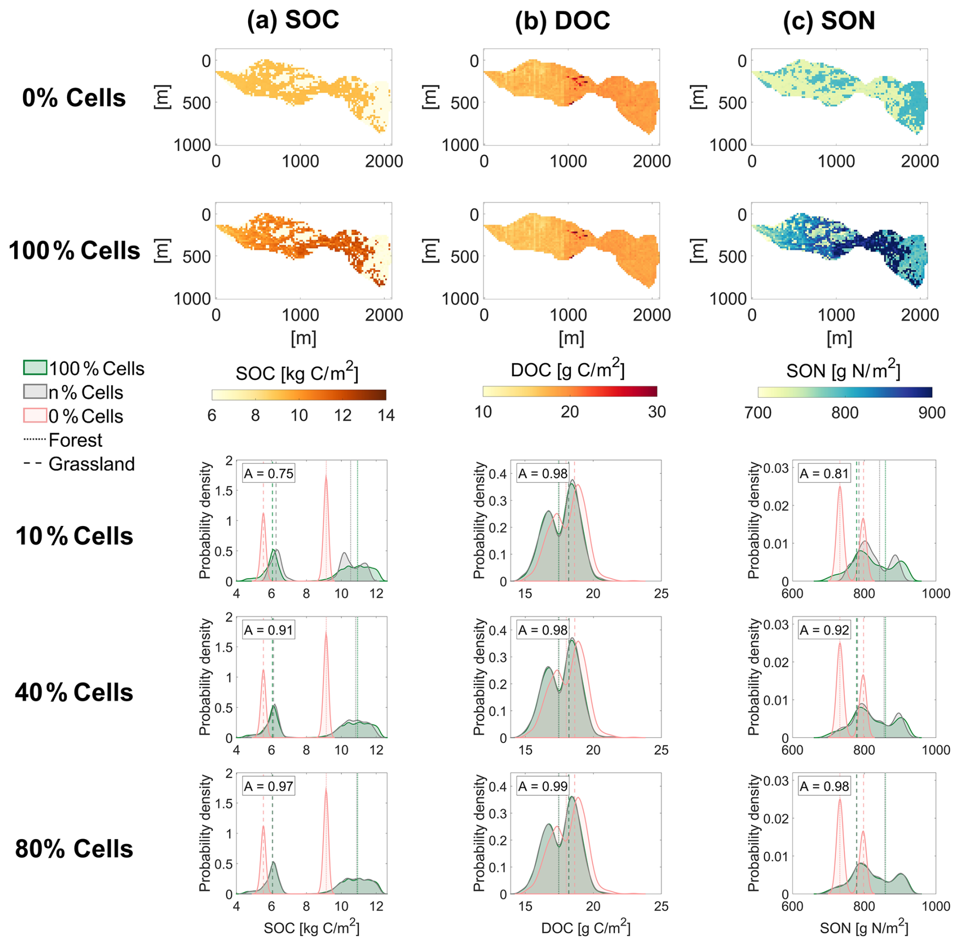
Figure 3 Spatial distributions of (a) soil organic carbon (SOC), (b) dissolved organic carbon (DOC), and (c) soil organic nitrogen (SON) in the Erlenbach catchment with the Original setup under two initialization conditions: with 0 % cell tracking (0 % Cells) and with 100 % cell tracking (100 % Cells). Probability density functions (PDFs) of each variable are shown for simulations using RF initialization with n=10 %, 40 %, and 80 %. Each is compared to the corresponding PDFs from the 0 % cells and 100 % cells simulations. The overlap area between PDFs (A value) is used to quantify the similarity between the RF-based distributions and the benchmark. Dashed and dotted lines represent median values for grassland and forest areas, respectively.

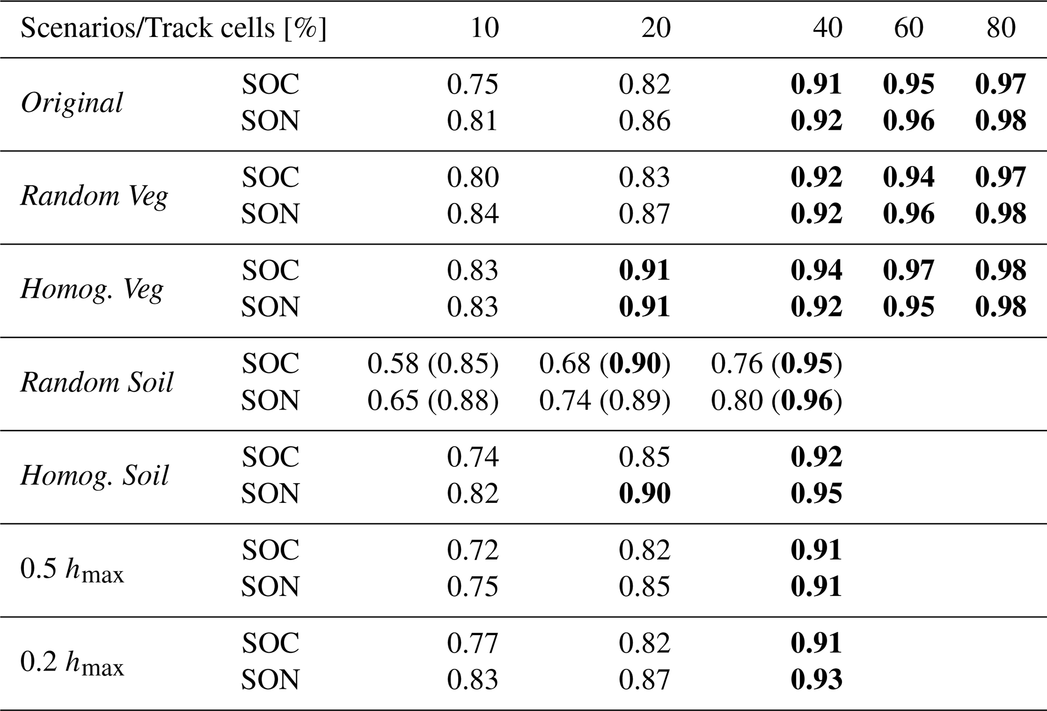
Interestingly, RF initialization using just n=10 % of the cells can reproduce approximately 75 % of the spatial variability in SOC (Fig. 3). Model performance improves with increasing percentages of tracked cells, and using n=80 % yields results that are nearly indistinguishable from the benchmark simulation. A notable performance jump occurs between n=20 % and 40 %. For example, in the Original simulation scenario, the overlap area (A value, quantifying the overlap between the PDFs of each simulation and the benchmark, with a value of A close to 1 indicating high similarity between distributions) increases from 0.82 to 0.91 for SOC and from 0.86 to 0.92 for SON (Table 2). Considering A≥0.9 as a threshold for satisfactory performance yields n=40 % of tracked cells being sufficient to accurately capture most of the spatial variability in SOC and SON (see Table 2) for the Original Erlenbach simulation scenario. Values of the Jensen–Shannon divergence, used to further compare similarities between PDFs, are reported in Table S4. Note, however, that the optimal percentage of tracked cells may vary depending on catchment characteristics such as vegetation composition, soil texture, topographic complexity, and background climate (see Sect. 3.2).

Table 2 Overlap area (A value) between the probability density functions (PDFs) of soil organic carbon (SOC) and soil organic nitrogen (SON) from different percentages of tracked cells and those from the benchmark simulation across multiple simulation scenarios. Values in parentheses under the Random Soil scenario represent results obtained when clay content was included as an additional predictor in the random forest model. Values greater than or equal to 0.90 are shown in bold.

Black lines in Fig. 4 show the temporal evolution of the coefficient of variation (CV, defined as the ratio of standard deviation to the mean) for spatial SOC under different RF initialization settings in forested and grassland areas (corresponding results for SON are provided in Fig. S5). In the n=0 % case, CV increases steadily over the 9-year simulation, indicating that spatial variability has not reached a steady state. In contrast, simulations initialized using the RF scheme maintain relatively stable CV values throughout the simulation period, with variability reflecting responses to dynamic environmental drivers rather than spin-up imbalance. CV values gradually increase across RF initialization settings with higher tracking percentages (n), approaching those of the benchmark. Notably, CV trajectories for RF settings using n=40 % and 100 % of tracked cells are nearly identical, confirming that n=40 % is sufficient to reproduce the full temporal dynamics of SOC spatial variability in the catchment here. Table S2 summarizes the robustness of the random forest models trained using 40 % of the tracked cells in the Original scenario. For most carbon and nitrogen pools, MAPE values are below 10 % and NRMSE values are below 0.1, indicating that the RF models exhibit satisfactory performance. These results provide direct support for H1, demonstrating that spatially explicit initialization is required to capture spatial variations of SOC and SON, as well as for H2, showing that spin-up at a subset of representative locations combined with RF extrapolation can satisfactorily reproduce benchmark dynamics.

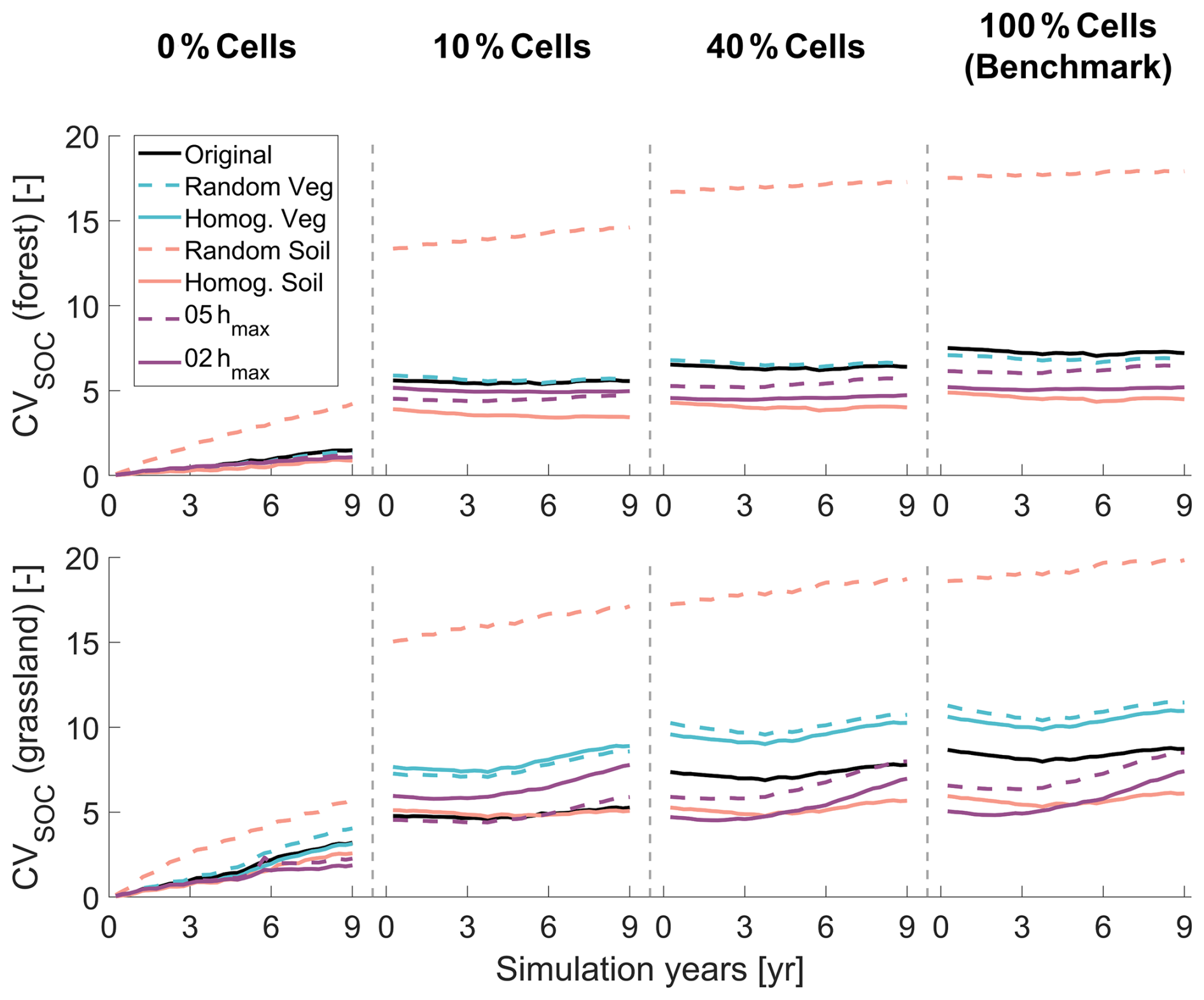
Figure 4 Temporal evolution of the coefficient of variation (CV) of spatial soil organic carbon (SOC) distribution over a 9-year simulation period in forest (top panels) and grassland (bottom panels) under different initialization settings and simulation scenarios. Each column represents one initialization setting: no cells tracking and no random forest (n=0 %), n=10 % cells tracking and random forest (10 % Cells), n=40 % cells tracking and random forest (40 % Cells), and n=100 % cells tracking (100 % Cells). Line colors and styles indicate results from different simulation scenarios, as shown in the legend.

3.2 Sensitivity across different catchment configurations

Table 2 and Fig. 4 also report the performance of using different n values in the RF model across different catchment configurations. Across all simulation scenarios, n=40 % can capture over 90 % of the spatial variability in both SOC and SON. An exception is observed in the Homog. Veg simulation scenario, where even n=20 % of tracked cells yields satisfactory performance.

A comparison among Original, Random Veg, and Homog. Veg simulations suggests that the number of tracked cells required for satisfactory RF performance is more sensitive to the proportion of vegetation types than to their spatial arrangement. As expected, when vegetation cover is spatially homogeneous, fewer cells are needed to achieve accurate predictions.

In contrast, results from the Original, Random Soil, and Homog. Soil simulations indicate that reducing the spatial heterogeneity of soil texture lowers the absolute spatial variability of SOC but does not necessarily reduce the number of tracked cells required for RF initialization. This is likely because soil texture is already included as a predictor in the RF model, and because in the Original scenario soil texture is relatively uniform (i.e., sand content: mean = 41 %, standard deviation = 2 % based on Gupta et al. (2024)). As a result, the model can capture soil-related variability effectively without the need for additional soil information. However, in the Random Soil scenario, where soil texture is highly heterogeneous, adding supplementary predictors such as the percentage of clay significantly improves the model’s ability to reproduce benchmark SOC spatial patterns (Table 2). This highlights the importance of including sufficient soil information when simulating spatial variability under heterogeneous soil conditions. Notably, the spatial CV is also higher in this scenario relative to the others, reflecting higher spatial variability of SOC. This is due to the expanded soil texture parameter space, especially variations in silt and clay contents, as this fine-particle-associated carbon contributes substantially to SOC (Six et al., 2002; Feng et al., 2013; Matus, 2021) (see also Table S5). These findings are consistent with previous studies showing that soil properties are among the most influential predictors in digital mapping of SOC (e.g., Meersmans et al., 2008; Zeraatpisheh et al., 2022; Martín-López et al., 2023).

Simulation results from the flatter topography scenarios (0.5 h_max and 0.2 h_max) indicate that a gentler topography does not necessarily lower the number of tracked cells needed for accurate RF initialization. In general, RF models require more samples when predictor distributions are not evenly distributed within their overall range of variation (e.g., when extreme values are underrepresented), in order to adequately represent the edges and tails of the input space (Peters et al., 2007; Simon et al., 2023). In our sampling design, the distributions of predictor variables were known in advance, and the selected cells were chosen to represent the full range of topographic and land cover features across the domain (Fig. S2). This targeted selection likely contributed to consistent RF performance across topographic conditions. It is also important to note that, in these simulations, the use of flatter topographies only results in reduced elevation differences, slopes, and curvatures, without altering the overall catchment shape, size, and contributing area, as the underlying catchment skeleton remains identical across scenarios. Additionally, the topographies were modified by tilting the surface around the lowest elevation point. While this can affect the average temperature values in the domain (and resulting absolute values of SOC and SON), it has no impact on the number of cells required within the same simulation configuration. Overall, these results highlight that the number of representative locations needed for satisfactory RF initialization is shaped by catchment-specific heterogeneity and predictor distributions, thereby supporting H3.

3.3 Bias analysis in relation to topography

Figure 5 presents the relationship between relative SOC bias ($\mathrm{\Delta }\mathrm{SOC}=({\mathrm{SOC}}_{\mathrm{simulation}}-{\mathrm{SOC}}_{\mathrm{benchmark}})/{\mathrm{SOC}}_{\mathrm{benchmark}}\times \mathrm{100}$) and the topographic wetness index (TWI) from the Original simulation scenario with n=0 %, 10 %, 20 %, 40 %, together with the PDFs of ΔSOC. Additional results covering all simulation scenarios are provided in Figs. S6 and S7.

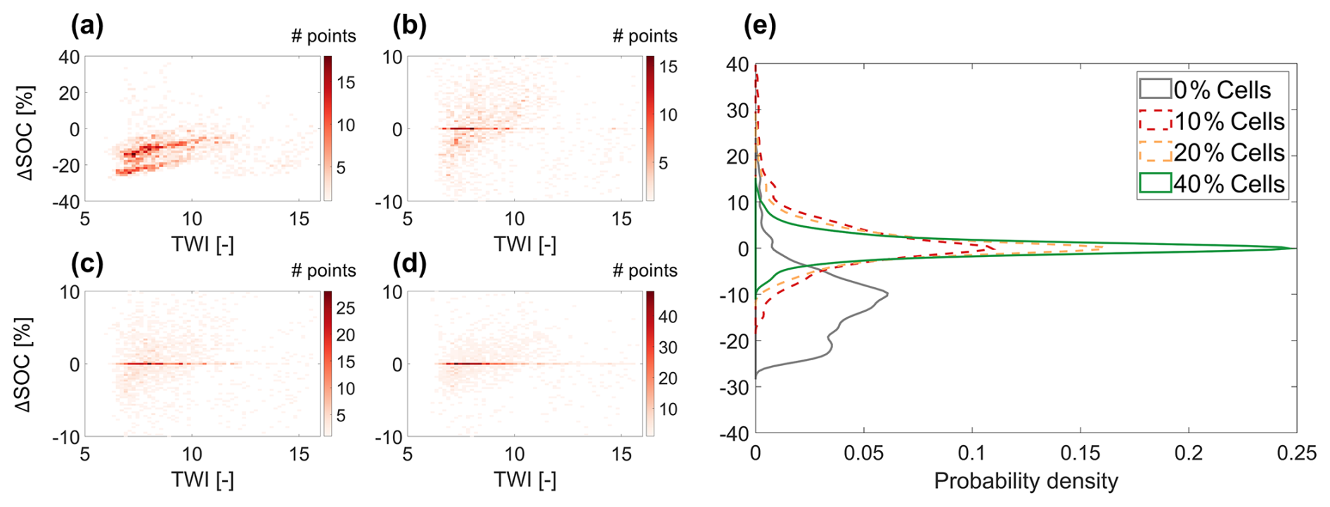
Figure 5 Density maps showing the relationship between relative SOC bias ($\mathrm{\Delta }\mathrm{SOC}=({\mathrm{SOC}}_{\mathrm{simulation}}-{\mathrm{SOC}}_{\mathrm{benchmark}})/{\mathrm{SOC}}_{\mathrm{benchmark}}\times \mathrm{100}$) and Topographic Wetness Index (TWI) under Original simulation scenarios with n = (a) 0 %, (b) 10 %, (c) 20 %, and (d) 40 %. (e) Probability density functions (PDFs) of ΔSOC from n=0 % (in gray), and with RF-based initialization using n=10 % (red dashed line), 20 % (yellow dashed line), and 40 % (green) of tracked cells.

Figure 5a shows that the n=0 % initialization configuration results in a systematic underestimation of SOC in many cells, with deviations reaching up to 20 %–30 % in some cases. This is because the initial pools (Fig. 2b) are derived from the 1D spin-up at the Erlenhöhe meteorological station, located at a relatively low elevation (1210 m a.s.l.) within the catchment. Since SOC generally increases with elevation due to temperature reductions (Parras-Alcántara et al., 2015; Teng et al., 2017; Zhu et al., 2019) – an effect captured by T&C-BG-2D (Lian et al., 2025b) – SOC in high-elevation areas gradually accumulates over time. However, the 9-year n=0 % simulation is insufficient for these areas to equilibrate, leading to a consistent underestimation (compared to the benchmark simulation, which instead captures the increasing trend of SOC with elevation) due to the lack of spatial information in the model initialization.

Interestingly, a positive relationship between ΔSOC and TWI is observed in the range TWI < 11, where the majority of grid cells are located (Fig. 5a). This trend can be explained primarily by the influence of water availability on soil respiration and, consequently, on SOC stocks. We note, however, that TWI is weakly but significantly correlated with elevation, and thus with air temperature ($r=-\mathrm{0.14}$, p<0.05). This suggests that temperature may also contribute to the observed relationship, although its influence is relatively minor compared to that of water availability. When the n=0 % initialization is applied, SOC exhibits almost no trend with TWI (Fig. 6a and b). However, the benchmark simulation shows a decreasing SOC trend with increasing TWI for TWI < 11, reflecting a long-term steady-state pattern shaped by soil respiration processes during spin-up. Simulations with n=10 % and n=40 % successfully capture the SOC–TWI relationship, with results from n=40 % being closer to the benchmark simulation. This relationship is consistent with previous findings showing an increase in soil respiration with water availability due to enhanced microbial activity (Manzoni et al., 2012, 2014; Yan et al., 2018), as shown in Fig. 6c and d. However, under excessively wet conditions (such as TWI > 11), this relationship reverses due to oxygen limitation (Moyano et al., 2013; Ruiz et al., 2015). Figure 6c and d further shows that while the n=0 % case reproduces the correct qualitative relationship between fast carbon fluxes (e.g., soil respiration) and TWI, correct flux magnitudes are only captured when n=10 % of the cells are tracked, and the performance is further improved for n=40 %. Because the SOC distribution in the benchmark simulation shows much higher spatial variability than in the n=0 % case, the decreasing SOC–TWI trend from the benchmark dominates the ΔSOC–TWI relationship, leading to an apparent positive correlation in Fig. 5a. The PDFs in Fig. 5e further confirm that the RF initialization scheme substantially reduces this topography-related bias. Using only n=10 % of the cells for RF training already eliminates most of the systematic bias (Fig. 5b), while n=20 % (Fig. 5c) and n=40 % (Fig. 5d) eliminate it almost entirely. The analysis here clearly highlights that the bias between plot-scale initialization and spatially-informed ones is strongly linked to grid-cell interactions via topography-controlled lateral transport.

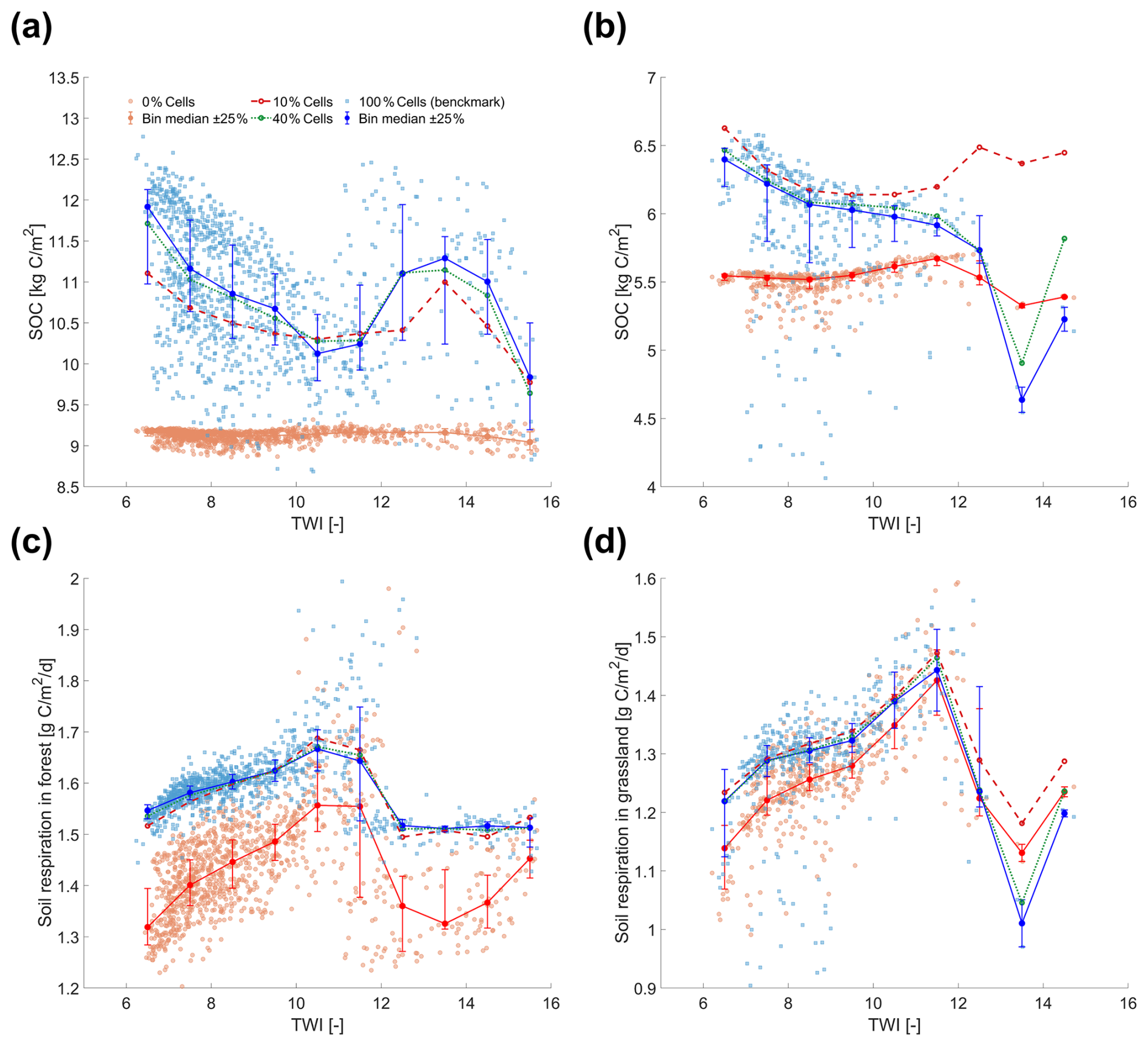
Figure 6 Relationship between the topographic wetness index (TWI) and (a, b) soil organic carbon (SOC) and (c, d) soil respiration in the Original simulation scenario, shown separately for forest (left) and grassland (right). Red points and lines represent results from n=0 % simulations; blue squares and lines show results from n=100 % simulations. Filled circles indicate the median values within TWI bins of width 1, with vertical bars showing the ±25 % range within each bin. Dashed red lines and dotted green lines present results from n=10 % and n=40 %, respectively.

3.4 The role of coupled vegetation dynamics in 1D soil biogeochemical spin-up

Figure 7 compares SOC values obtained from different simulation stages and spin-up strategies. The first column represents the initial SOC values (here, values in Fig. 2b are used, but can be derived from the steady state in areas with similar land cover, soil, and climatic conditions, or from a reasonable initial guess). The next three columns show SOC values after 9, 18, and 27 years of simulation using the full T&C-BG model (i.e., with coupled soil biogeochemical and vegetation dynamics). These three columns are used to exemplify the gradual convergence of SOC toward steady-state conditions. The gray box in the middle shows the SOC state obtained using the biogeochemistry-only spin-up with 9-year average vegetation fluxes after 1000 years (i.e., no coupled vegetation dynamics – equivalent to step (a) in Fig. 2). Starting from this uncoupled spin-up steady state, an additional 27 years of simulation (3×9 years) were performed using the full T&C-BG model, with results shown in the three subsequent central columns. Such trajectories should not be interpreted as generally indicative of the direction toward the final steady state, as SOC and SON may follow non-monotonic pathways in dynamic systems. In the present simulations, however, both SOC and SON evolve toward the long-term coupled reference steady state during the first 27 years. The red box on the far right indicates the reference steady state achieved through long-term simulation with the fully coupled T&C-BG model, which considers the coupled vegetation-soil biogeochemistry dynamics. Each boxplot includes five representative sites with different vegetation types (see Fig. 2h). Site-specific vegetation and soil information, along with SOC and SON pool sizes, are provided in Table S3. A corresponding analysis for SON is shown in Fig. S8.

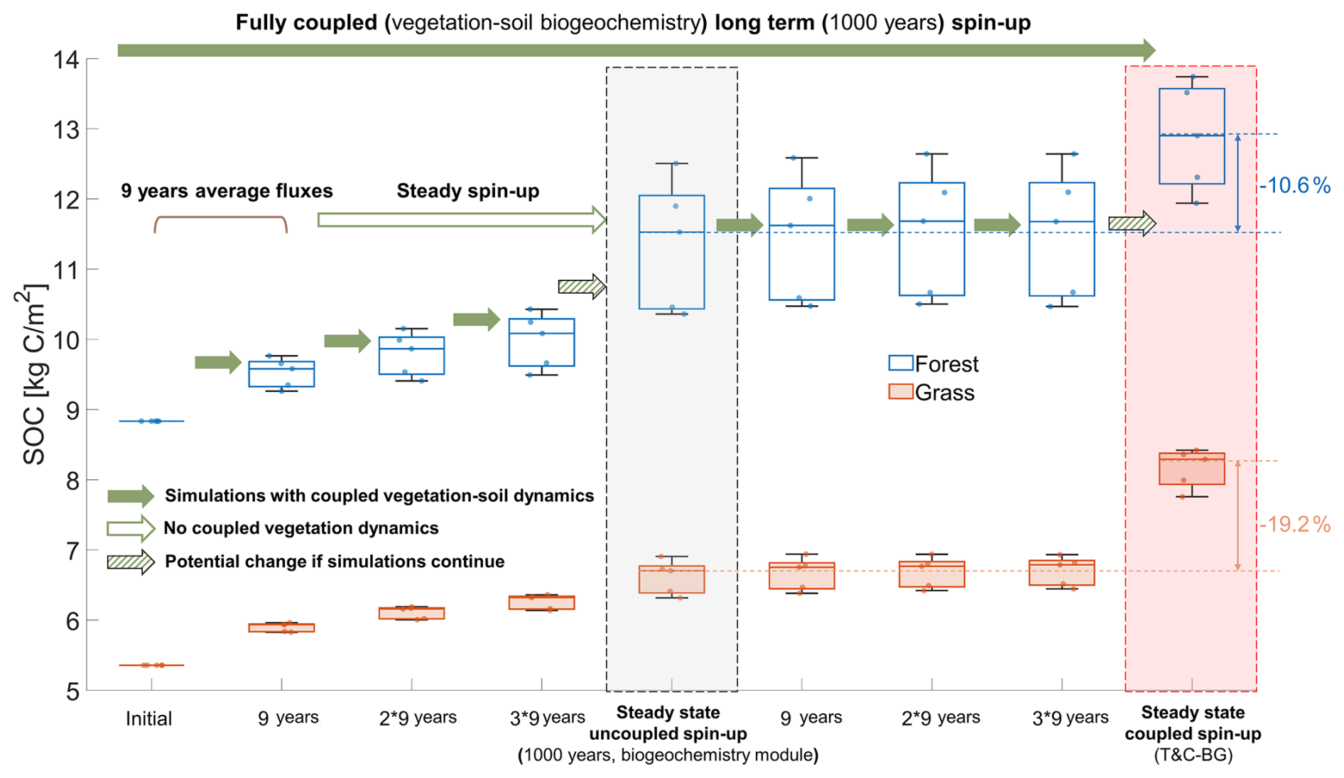
Figure 7 Evolution of soil organic carbon (SOC) during different initialization schemes and simulation durations at 10 selected sites (Fig. 2h). Blue/orange boxplots represent forest/grassland sites. Arrows indicate simulation transitions between stages. The initial values (far left) are followed by 3×9-year simulations using the fully coupled T&C-BG model (solid green arrows). The average vegetation fluxes are extracted from the first 9 years to obtain a steady-state condition with the biogeochemistry-only module (outlined green arrow, middle gray box). This is followed by three additional 9-year simulations. A comprehensive long-term spin-up using the fully coupled T&C-BG model (i.e., considering coupled vegetation and soil biogeochemical dynamics) is shown in the right red box. Striped arrows indicate the potential direction of SOC change if coupled simulations continue beyond the current duration.

As shown in Fig. 7, the initial SOC values are substantially underestimated in the case here and gradually increase over the course of the simulation. After a 27-year simulation period with the fully coupled T&C-BG model, the resulting SOC is still largely underestimated compared to the long-term steady state (red shading). Reaching steady state with the fully coupled model would require approximately 1000 years. A direct comparison of SOC between the uncoupled spin-up steady state (middle gray box in Fig. 7) and the reference steady state from the fully coupled plot-scale spin-up (red shading) reveals an average underestimation of 19.2 % and 10.6 % for grassland and forested sites, respectively (see also Table S3). The underestimation is further reduced for the case of SON (see Fig. S8). This uncoupled spin-up steady state can be reached by first running the fully coupled model for only a short period (here 9 years) to obtain average vegetation fluxes, which are then used to drive the biogeochemistry-only spin-up. This provides a substantial gain in computational efficiency, as the computation time for decoupled spin-up is negligible (Table S6) despite the slight disagreement in steady states, thus supporting the choice of adopting an uncoupled spin-up approach as a first step (Fig. 2a) within the proposed initialization framework and confirming H4.

In summary, the domain used here contains 1859 cells in total. Tracking lateral fluxes in all cells increases computational cost significantly (e.g., by approximately 50 % compared to a simulation without tracking any fluxes when n=20 %), whereas tracking only n=10 % of the cells has a less than 10 % impact on the overall spin-up procedure (Table S6). In Erlenbach, SOC requires over 300 years of simulation to reach steady state (Fig. S9) even without coupled vegetation-soil biogeochemical dynamics. The proposed initialization framework reduces this demand by collapsing the full 300-year 2D spin-up into two 9-year simulations (corresponding to Fig. 2b and f), combined with a 1D plot-scale spin-up. Ideally, the hybrid spin-up procedure requires two 9-year 2D simulations instead of 300 years (i.e., 18 years in total, corresponding to approximately 6 % of the original simulation length). Wall-clock times of different components of the spin-up procedure are reported in Table S6. While these times are expected to change based on the specific computational platform used, for the case here the hybrid spin-up procedure resulted in a computational saving of approximately 90 % using the recommended n=40 % configuration.

4 Discussion

Overall, our experiments confirm the four hypotheses outlined in the Introduction. Spatially explicit spin-up is necessary to capture spatial variability in soil carbon and nutrient pools (H1), while RF-based extrapolation from a subset of representative cells provides an efficient and accurate alternative to a fully distributed spin-up (H2). The required sampling fraction is not universal (H3) but depends on catchment-specific heterogeneity and the choice of predictors. Finally, an uncoupled biogeochemistry-only spin-up offers a computationally efficient first step (H4), yielding steady states sufficiently close to the fully coupled solution, hence justifying its use in practical applications. Beyond the associated computational savings, this framework incorporates lateral transport between computational cells during spin-up, explicitly accounting for topography-induced lateral water redistribution. In this respect, it differs from more conventional grouped representations of landscape heterogeneity in hydrological and land surface models, such as hydrological response units (HRUs), tiles, or other classes of cells sharing similar characteristics (e.g., Chaney et al., 2018; Yang et al., 2025; Verhoef et al., 2026).

The approach proposed here is not limited to T&C-BG-2D but can be readily applied to the initialization of other spatially distributed ecohydrological-soil biogeochemical frameworks. Many such models (e.g., RHESSys, Tague and Band, 2004; Flux-PIHM-BGC, Shi et al., 2018) couple a hydrological component with a plot-scale vegetation and/or soil biogeochemistry module. In these systems, lateral transport of water and carbon can be tracked and incorporated into the plot-scale spin-up, which can then be combined with a RF algorithm for initialization across the entire catchment.

The Erlenbach catchment served here as a testbed to evaluate the effectiveness of the new initialization scheme. For this site, tracking only 40 % of the cells was sufficient for the RF model to reconstruct over 90 % of the spatial variability in key soil biogeochemical variables. However, this proportion (40 %) should not be interpreted as a universal threshold. Our scenario experiments indicate that the optimal percentage is catchment-dependent and shaped by the degree of heterogeneity in vegetation, soils, and topography. For instance, in the Homog. Veg scenario even 20 % of tracked cells were sufficient, whereas in the Random Soil scenario, additional soil predictors were needed to adequately capture SOC variability. Flatter topographies here did not necessarily reduce the required sample size, because the contributing area remained largely unchanged and soil–vegetation heterogeneity still needed to be sufficiently represented in the sampling. Sensitivity analysis suggests that vegetation type is the most important predictor in the RF model. Taken together, these findings indicate that the sampling fraction required for effective RF initialization depends on specific catchment characteristics. In particular, it is influenced by the level of heterogeneity in the landscape, the unevenness of RF predictor distributions, and the number and type of predictors considered (e.g., inclusion of additional soil information or vegetation attributes).

A sensitivity analysis of predictor importance in the RF model indicates that the type of vegetation is the most influential variable (Fig. S10), followed by elevation. This statement is further confirmed by the Shapley values reported in Tables S2 and S3. These findings align with previous studies showing that vegetation strongly influences the spatial distribution of SOC (e.g., Kunkel et al., 2022; Yao et al., 2023) and that elevation is a dominant control in pronounced topographies such as Erlenbach because of the lapse rate control on air temperature (Stähli et al., 2021; Lian et al., 2025b). The relative importance of these predictors may vary in catchments with different climatic and topographic characteristics. Note that soil texture is relatively less important in the sensitivity analysis in Fig. S10. This is likely due to the relatively homogeneous soil texture distribution in Erlenbach. However, the Random Soil scenario (Sect. 3.2) highlight the essential role of including soil information among the RF predictors, particularly in areas characterized by high soil spatial variability. Shapley values in Table S5 show that clay content is the most important predictor (after vegetation type) for soil carbon prediction, suggesting that clay content should be explicitly considered in generalized RF modeling frameworks.

While the proposed framework performs robustly in our tests, a few aspects deserve special attention and should be considered for applications in specific cases. In this study, the average soil texture was used in step (a) of the initialization procedure (Fig. 2) for the Random soil scenario, and the resulting steady-state conditions were assigned to all cells. This simplification may introduce a potential bias, because soil textures can alter the degree of water limitation experienced by vegetation, plant fluxes, and ultimately the initialization outcome. To evaluate this effect, we tested three soil texture settings (sand (60 % sand, 10 % clay), loam (40.5 % sand, 26.5 % clay), and clay (20 % sand, 50 % clay)) in step (a) of Fig. 2, and found that the resulting initialization states and spatial distributions are largely unchanged (see Fig. S11). However, this is likely due to the fact that vegetation in Erlenbach does not experience water limitation. Conversely, in drier regions, soil texture could become a major constraint and separate spin-ups for each soil type may be required instead of using an average soil texture. Apart from soil texture, we did not include elevation-based clusters in step (a) of the initialization procedure (Fig. 2), which is potentially necessary if the catchment has significant elevation changes or it spans climatic regimes where processes such as permafrost occurrence or soil freezing are relevant. Furthermore, soil–vegetation coupling is inherently site-specific, and the decoupled spin-up here relies on a 9-year average of plant and soil dynamics. While this assumption is reasonable for the Erlenbach site, it may introduce biases in more extreme ecosystems (e.g., nutrient-limited environments, more variable climatic conditions), where long-term average plant-soil biogeochemical dynamics cannot be adequately captured within a 9-year period. We therefore suggest evaluating this assumption by running longer-term simulations for a small subset of grid cells and verifying that the plant-soil dynamics averaged over the chosen period do not introduce systematic biases relative to longer-term simulations. In addition to the sensitivity analysis discussed in the previous paragraphs, we recommend that, when implementing the proposed spin-up procedure in a new case study, the first step should be to assess the distribution of key environmental predictors in the study area (particularly vegetation type and soil texture) and to apply a proper sampling strategy to represent the predictor space. In more heterogeneous catchments, the sampling strategy could be extended by stratifying not only by vegetation type, but also by additional gradients such as elevation and soil type. The adequacy of the sampling can then be assessed by verifying whether the selected cells sufficiently cover the predictor space. It is also essential to evaluate whether the ecosystem is nutrient-limited and whether the meteorological forcing is representative of the long-term climatic conditions. Based on these considerations, a tracked-cell proportion of n=10 %–40 % may serve as an initial guideline, with the final choice determined by the trade-off between target accuracy and available computational resources.

The initialization scheme proposed here provides steady-state initial conditions. This is indeed a convenient simplification (often adopted in soil biogeochemical modeling), which may not always be realistic, especially over long timescales and in certain contexts (e.g., long-term vegetation colonization, young forest development, post-disturbance recovery after wildfires; Guo and Gifford, 2002; Ilstedt, 2003; Nave et al., 2011; Zhang et al., 2023). To apply the proposed approach in systems that are not in steady state, a possible strategy is to assume a pre-disturbance steady state, derive the initial conditions from that point, and then iteratively apply the initialization scheme over shorter time intervals. For example, in an area undergoing young forest growth, the initial condition may be approximated from the land use prior to forest establishment. A short-term simulation (e.g., 1 year) can then be used to obtain average plant fluxes. These fluxes can be applied in a longer simulation period (e.g., 5 years), followed by another short-term run to update the fluxes. This process introduces a loose coupling between vegetation dynamics and soil biogeochemistry, allowing the model to gradually adjust toward a consistent state. The simulation–flux update cycle can be repeated until model outputs align with observations. In such cases, only the 1D spin-up component of the initialization scheme requires modification, while the RF algorithm remains applicable without change. However, if only part of the catchment is affected by disturbance, separate RF models may be needed for disturbed and undisturbed regions.

5 Conclusions

This study presents a novel initialization scheme for spatially distributed coupled ecohydrological-soil biogeochemical models, integrating a flux-tracking spin-up with a RF algorithm, thus contributing to ongoing efforts in the development and reliable application of fully coupled spatially distributed models. Our results underscore the importance of explicitly accounting for lateral fluxes and spatial heterogeneities in model initialization for reducing systematic biases in modeled patterns of soil carbon and nutrients. The proposed framework achieves a dynamic steady state efficiently and demonstrates robust performance of the RF model, which required tracking lateral fluxes for only a relatively limited number of cells to effectively represent spatial variability in the setup of initial conditions for carbon and nutrient pools. The number of cells required for lateral flux tracking is primarily determined by the spatial complexity of the catchment and the amount of spatial information contained in the predictors used in the RF model. While demonstrated using T&C-BG-2D, the methodology proposed here is broadly applicable to other spatially distributed models, offering an efficient framework to improve the accuracy of distributed soil biogeochemical models by explicitly including spatial information in their spin up and initialization, while maintaining a reasonable computational effort. This will ultimately enhance not only our ability to reproduce spatial patterns of soil carbon and nutrients at the catchment scale but also our understanding of the role of topography in modulating coupled processes related to water, energy, and biogeochemical fluxes in complex landscapes.