The Normalized Interpolated Convolution from an Adaptive Subgrid (NICAS) method

This article presents an innovative method to apply a correlation operator to a vector in a high-dimensional system, as often needed in variational data assimilation algorithms. The Normalized Interpolated Convolution from an Adaptive Subgrid (NICAS) method is very appealing as it can work for any grid, on domains with complex boundaries, producing inhomogeneous and anisotropic correlation functions, and it is very efficient for large correlation support radii. In this study, we detail the method motivations and theoretical background, we describe the practical implementation of several important features, and we assess its computational cost in various configurations to exhibit its strengths and limitations. Finally, we compare these characteristics to the similar existing methods.

1 Introduction

In variational data assimilation, the background error term of the minimized cost function requires the application of a background error covariance matrix. Due to the size of the system, this matrix is never stored and applied directly, but modeled using different techniques, so it is referred to as “operator” rather than “matrix” hereafter. While the inverse of the background error operator generally appears in the cost function, only its forward application or the application of one of its square-roots is needed in minimization algorithms, thanks to preconditioning techniques.

We can distinguish two broad classes of background error covariance operators:

1. Parametrized covariance operators are built as sequences of sparse operators (see Bannister, 2008a, b for a detailed review), where the central operator is a univariate correlation operator.

2. Ensemble-based covariance operators are directly sampled from an ensemble of forecasts, and the sampling noise is damped with a localization operator, which has the structure of a correlation operator (Lorenc, 2003; Buehner, 2005).

In both cases, it is thus necessary to apply a correlation operator to a vector, and this operation has to be performed many times: as many as the number of iterations in the minimization for a parametrized covariance operator (∼10²), and as many as the number of iterations in the minimization multiplied by the ensemble size for the ensemble-based operator (∼10⁴). As a consequence, applying the correlation operator must be fast and scalable. Many methods have already been developed to achieve this, all with their own strengths and limitations, as described in the Discussion section at the end of this paper.

The Normalized Interpolated Convolution from an Adaptive Subgrid (NICAS) presented here can work on any model grid, regular or unstructured, it can handle domains with complex boundaries like oceans, land-surface or sea-ice models, it can represent inhomogeneous and anisotropic correlation functions without any additional cost, and it is particularly efficient for large correlation support radii.

The NICAS method was initially developed in 2017, and a first note was published without peer review three years later (Ménétrier, 2020). Since then, the method and its implementation have been continuously improved within the BUMP (Background error on an Unstructured Mesh Package) block of the SABER (System-Agnostic Background Error Representation) library, a keystone of the JEDI (Joint-Effort for Data assimilation Integration) project lead by the JCSDA and its partners. The current code is more mature and very different from what it was in 2020, and it is now routinely used in research and operations by many users (Liu et al., 2022; Guerrette et al., 2023; Jung et al., 2024).

The scope of this article is limited to univariate aspects of correlation operators: the NICAS method does not handle the correlations between variables in multivariate cases. In most variational data assimilation systems, univariate and multivariate aspects are separated. For correlation operators, so called “balance operators” can introduce complex relationships between variables, as described for the atmosphere in Bannister (2008a, b) for large scales and Bannister (2021) for convective scales, or as in Weaver et al. (2005) for the ocean. For localization operators, the multivariate treatment is often simpler, as described in Ménétrier (2023) and Lee et al. (2024).

The NICAS method, its motivations and features are described in Sect. 2, while the practical implementation challenges and choices are explained in Sect. 3, with a step-by-step illustration of the resulting algorithm. In Sect. 4, we evaluate the performances of the NICAS method for different configurations and we assess the scalability of the different tasks. An overview of the similar existing methods is given in Sect. 5, to underline for which applications and configurations each method should be preferred, before the conclusions in Sect. 6.

2 NICAS method description

2.1 Motivations

To introduce the NICAS method, we start with a brief order-of-magnitude analysis of the computational cost of the application of a correlation matrix to a vector. Let us assume that a domain of dimensionality k (e.g. k=2 on a plane or on the sphere) is discretized into a grid 𝒢 containing n cells of typical size γ and typical volume proportional to γ^k. Since the total volume of the domain 𝒱∝nγ^k is fixed, we can deduce that $n\propto {\mathit{\gamma }}^{-k}$. Applying a dense correlation operator $\mathbf{C}\in {\mathbb{R}}^{n\times n}$ to a vector x∈ℝⁿ requires 𝒦∝n² operations, which is not computationally affordable for large systems (e.g. n∼10⁹ for NWP operational systems).

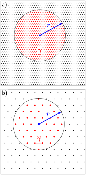
However, as illustrated on the plane (k=2) in Fig. 1a, if the correlation function defining C is compactly supported with a typical support radius r, the number of points within the support is proportional to r^k≪𝒱 and C becomes sparse. The number of operations 𝒦 can be be significantly reduced: 𝒦∝r^kn instead of n². Introducing the correlation resolution $\mathit{\rho }=r/\mathit{\gamma }$, i.e. the correlation support radius r expressed as a function of the grid cell size γ, we finally get 𝒦∝ρ^k. In many cases, ρ is rather large. For instance, a 300 km correlation support radius for a 10 km resolution grid gives a correlation resolution ρ=30.

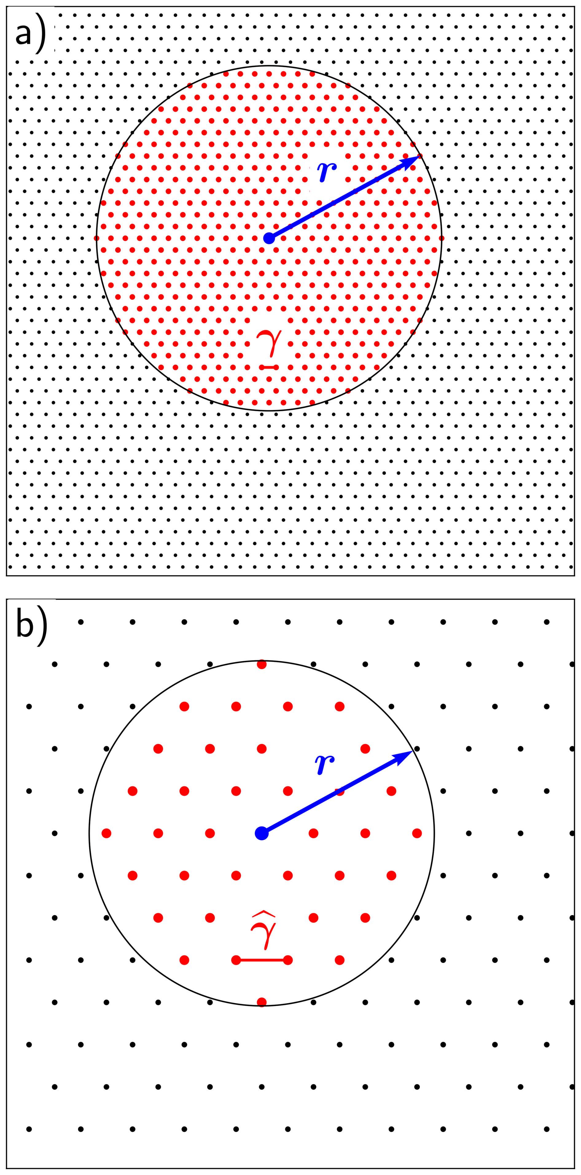
Figure 1 Example on the plane of a full grid (a) and a subgrid (b), with cells of typical size γ or $\widehat{\mathit{\gamma }}$, respectively. The red dots are involved in the convolution with a correlation function of radius r of the blue point at the center. The number of operations required to apply the convolution over the whole domain is obviously larger in case (a) than in case (b), and is proportional to the of the correlation resolutions $r/\mathit{\gamma }$ and $r/\widehat{\mathit{\gamma }}$ squared, respectively.

The fundamental idea of the NICAS method, as illustrated in Fig. 1b, is to apply the correlation operator on a dedicated subgrid $\widehat{\mathcal{G}}$ of size $\widehat{n}$ and typical cell size $\widehat{\mathit{\gamma }}$, for which the correlation resolution $\widehat{\mathit{\rho }}=r/\widehat{\mathit{\gamma }}$ is minimal, in order to reduce the number of operations from 𝒦∝ρ^k to $\widehat{\mathcal{K}}\propto {\widehat{\mathit{\rho }}}^k$. However, $\widehat{\mathit{\rho }}$ should be large enough to keep the correlation function sharpness on $\widehat{\mathcal{G}}$. To define this adaptive subgrid $\widehat{\mathcal{G}}$, we start from the correlation resolution $\widehat{\mathit{\rho }}$ prescribed by the user, from which we deduce the typical subgrid cell size $\widehat{\mathit{\gamma }}=r/\widehat{\mathit{\rho }}$.

The NICAS correlation operator C on the grid 𝒢 is given by

$$\begin{array}{}\text{(1)}& \mathbf{C}=\mathbf{NS}\widehat{\mathbf{C}}{\mathbf{S}}^{\mathrm{T}}{\mathbf{N}}^{\mathrm{T}}\end{array}$$

where $\widehat{\mathbf{C}}\in {\mathbb{R}}^{\widehat{n}\times \widehat{n}}$ is the correlation operator on $\widehat{\mathcal{G}}$, $\mathbf{S}\in {\mathbb{R}}^{n\times \widehat{n}}$ is an interpolation from $\widehat{\mathcal{G}}$ to 𝒢, $\mathbf{N}\in {\mathbb{R}}^{n\times n}$ is a diagonal operator ensuring that C is normalized (i.e. C_ii=1), because even if $\widehat{\mathbf{C}}$ is normalized, $\mathbf{S}\widehat{\mathbf{C}}{\mathbf{S}}^{\mathrm{T}}$ is not normalized in general.

If ρ is large enough, then $\widehat{\mathit{\rho }}$ can be set a value significantly smaller than ρ, in which case the cost of the NICAS method should become dominated by the interpolation S, which grows linearly with n. Another important feature of the NICAS approach is the large flexibility given to $\widehat{\mathbf{C}}$, which is fully explicit. Thus, it can be inhomogeneous and anisotropic, non-separable, and handle complex boundaries. A final key aspect is the subgrid adaptiveness: the local density of $\widehat{\mathcal{G}}$ should be a function of the local correlation support radius of $\widehat{\mathbf{C}}$.

2.2 Working with square-roots

Since $\widehat{\mathbf{C}}$ is a correlation operator, it is symmetric positive definite. Thus, there is an infinity of possible square-roots $\widehat{\mathbf{U}}\in {\mathbb{R}}^{\widehat{n}\times m}$ such that $\widehat{\mathbf{C}}=\widehat{\mathbf{U}}{\widehat{\mathbf{U}}}^{\mathrm{T}}$. The number m of columns of $\widehat{\mathbf{U}}$ depends on the chosen modeling for $\widehat{\mathbf{U}}$. Once $\widehat{\mathbf{U}}$ is defined, it is straightforward to provide a square-root of C denoted $\mathbf{U}\in {\mathbb{R}}^{n\times m}$:

$$\begin{array}{}\text{(2)}& \mathbf{U}=\mathbf{NS}\widehat{\mathbf{U}}.\end{array}$$

In practice, it is always better to implement U and U^T than C directly, for at least two reasons:

• ensuring the positive definiteness of the implementation of C can be numerically challenging, while UU^T is always symmetric positive (semi-)definite by construction,

• U can be very useful for cost function preconditioning, or in randomization procedures to generate an ensemble of perturbations whose asymptotic correlation matrix is C.

2.3 The Gaspari and Cohn (1999) function square-root

The shape of the correlation function in $\widehat{\mathbf{C}}$ is completely free in the NICAS method, as long as its square-root is known. However, we have chosen to stick to the widely used piecewise polynomial, compactly supported function from Gaspari and Cohn (1999), denoted GC99 hereafter. For sake of simplicity, a slightly different scaling is used in this function compared to the original paper (Sect. 4c), to ensure that it goes to zero when the input argument goes to one:

$$\begin{array}{}\text{(3)}& \begin{array}{rl}& \mathcal{C}\left(d\right)=\\ & \left\{\begin{array}{ll}\mathrm{1}-\mathrm{8}{d}^{\mathrm{5}}+\mathrm{8}{d}^{\mathrm{4}}+\mathrm{5}{d}^{\mathrm{3}}-\frac{\mathrm{20}}{\mathrm{3}}{d}^{\mathrm{2}}& \mathrm{if}d\le \frac{\mathrm{1}}{\mathrm{2}}\\ {\displaystyle \frac{\mathrm{8}}{\mathrm{3}}}{d}^{\mathrm{5}}-\mathrm{8}{d}^{\mathrm{4}}+\mathrm{5}{d}^{\mathrm{3}}+{\displaystyle \frac{\mathrm{20}}{\mathrm{3}}}{d}^{\mathrm{2}}-\mathrm{10}d+\mathrm{4}-{\displaystyle \frac{\mathrm{1}}{\mathrm{3}}}{d}^{-\mathrm{1}}& \mathrm{if}\frac{\mathrm{1}}{\mathrm{2}}<d\le \mathrm{1}\\ \mathrm{0}& \mathrm{if}\mathrm{1}<d\end{array}\right..\end{array}\end{array}$$

Here, the normalized distance d corresponds in the original paper to $\left|z\right|/\mathrm{2}c$ where $\left|z\right|$ is the distance to the origin and c is the half support radius. As explained in the original paper, this function is obtained “by self-convolving the continuous, piecewise linear function”, which provides an explicit square-root function 𝒰(d). Within the more general parametric family developed in the original paper, the special case of 𝒞(d) corresponds to a linear square-root function 𝒰(d):

$$\begin{array}{}\text{(4)}& \mathcal{U}\left(d\right)=\left\{\begin{array}{ll}\mathrm{1}-\mathrm{2}d& \mathrm{if}d\le \frac{\mathrm{1}}{\mathrm{2}}\\ \mathrm{0}& \mathrm{if}\frac{\mathrm{1}}{\mathrm{2}}<d\end{array}\right..\end{array}$$

In the discrete case, the correlation square-root $\widehat{\mathbf{U}}$ is built as:

$$\begin{array}{}\text{(5)}& {\widehat{U}}_{ij}=N_i^{\prime }\mathcal{U}\left(d_{ij}\right)\mathrm{with}{d}_{ij}={\displaystyle \frac{\mathcal{Z}(i,j)}{r}}\end{array}$$

where 𝒵(i,j) is a measure of the distance between the points of $\widehat{\mathcal{G}}$ corresponding to indices i and j, and $N_i^{\prime }$ is an internal normalization factor ensuring that ${\widehat{C}}_{ii}=\mathrm{1}$. Figure 2 illustrates this correlation function on a regular 1D subgrid, with a correlation resolution $\widehat{\mathit{\rho }}=\mathrm{8}$:

• A vector δ of impulses is defined on $\widehat{\mathcal{G}}$ (δ_i=0 except for a few elements where δ_i=1).

• The correlation square-root adjoint ${\widehat{\mathbf{U}}}^{\mathrm{T}}$ is applied on δ, showing the triangular shape defined in equation (4).

• The correlation $\widehat{\mathbf{C}}=\widehat{\mathbf{U}}{\widehat{\mathbf{U}}}^{\mathrm{T}}$ is applied on δ, showing the discrete approximation of the bell shape defined in Eq. (3).

It should be noted that the internal normalization N^′ works as intended: reducing the amplitude of $\widehat{\mathbf{U}}$ with an appropriate factor leads to a perfectly normalized $\widehat{\mathbf{C}}$.

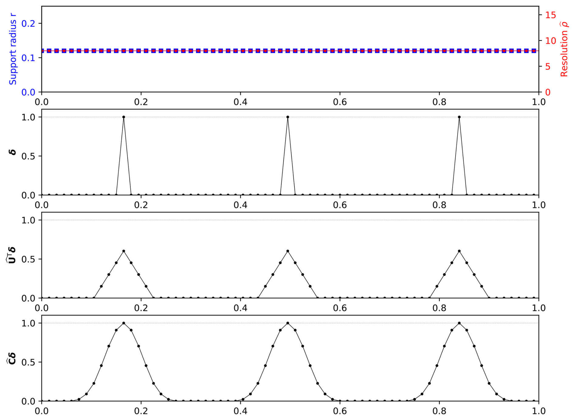
Figure 2 Correlation operator applied to impulses on a 1D subgrid. From top to bottom: support radius r and correlation resolution $\widehat{\mathit{\rho }}$; vector of impulses δ; correlation square-root adjoint applied to impulses ${\widehat{\mathbf{U}}}^{\mathrm{T}}\mathit{\delta }$; correlation applied to impulses $\widehat{\mathbf{C}}\mathit{\delta }$.

2.4 Anisotropic extension

If the domain dimensionality k is larger than 1, the correlation operator can be made anisotropic by replacing the normalized distance d_ij in Eq. (5) with a tensor-based normalized distance:

$$\begin{array}{}\text{(6)}& d_{ij}=\sqrt{\left(\mathit{x}\right(i)-\mathit{x}(j\left){)}^{\mathrm{T}}{\mathbf{D}}^{-\mathrm{1}}\right(\mathit{x}\left(i\right)-\mathit{x}\left(j\right))}\end{array}$$

where x(i)∈ℝ^k is the vector of coordinates of the point of $\widehat{\mathcal{G}}$ corresponding to index i, $\mathbf{D}\in {\mathbb{R}}^{k\times k}$ is a support tensor. In Weaver and Mirouze (2013), the local correlation tensor is described as “a natural generalization of the (square of) the Daley length-scale for characterizing the spatial scales of the function”. Similarly here, the support tensor D is a natural generalization of the support radius r of the GC99 function. The components of D define the support of the function as a k-dimensional ellipsoid. Figure 3 shows examples of the GC99 function with different support tensors in a 2D case.

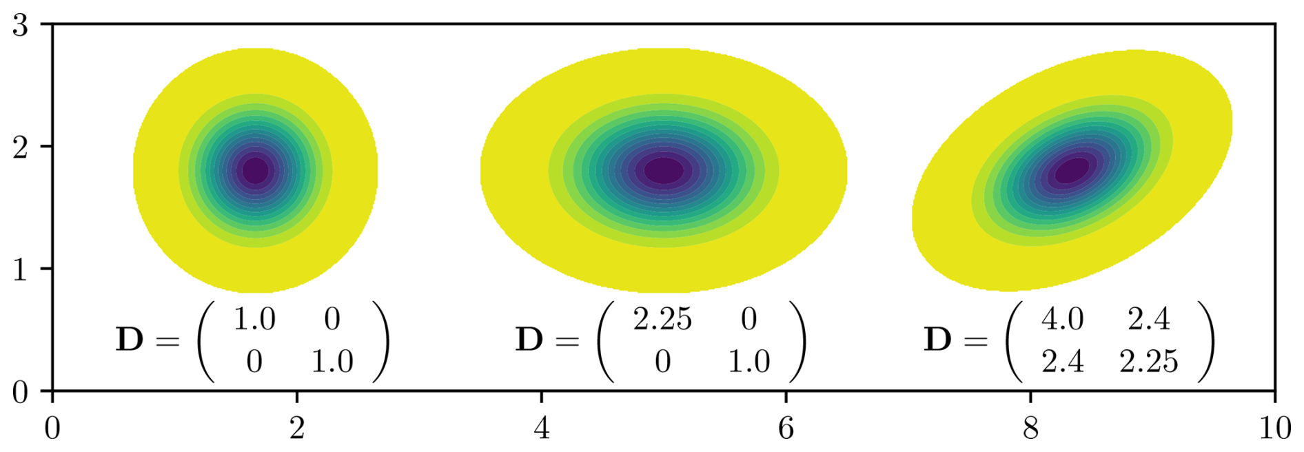
Figure 3 Examples of anistropic GC99 functions with three different support tensors, in the cartesian (x, y) coordinates system.

2.5 Multi-components extension

To change the shape of the correlation function, two strategies are possible:

• either using another correlation function for 𝒞(d), but a square-root 𝒰(d) must be explicitly available,

• or combining several components of the GC99 function together, with a specific support radius and a specific weight for each component.

Figure 4 shows an example of the second approach: three components with decreasing support radii and increasing weights are combined to produce a peaked correlation function with fat tails. In this case, the overall computational cost is dominated by the component with the smaller support radius.

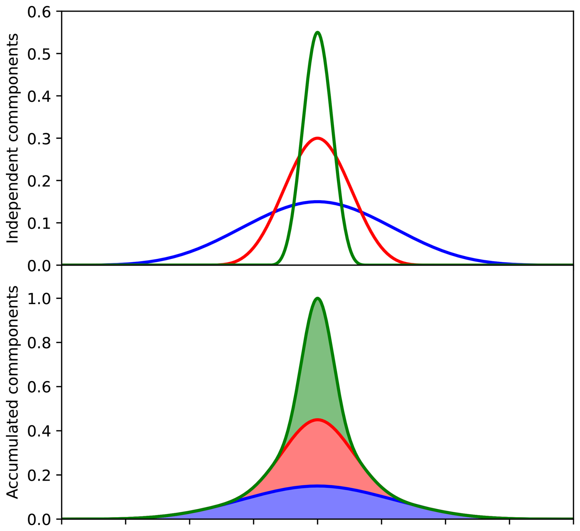
Figure 4 Three NICAS components with decreasing support radii and increasing weights, separated (top panel) or combined (bottom panel).

2.6 Inhomogeneous extension with an adaptive subgrid

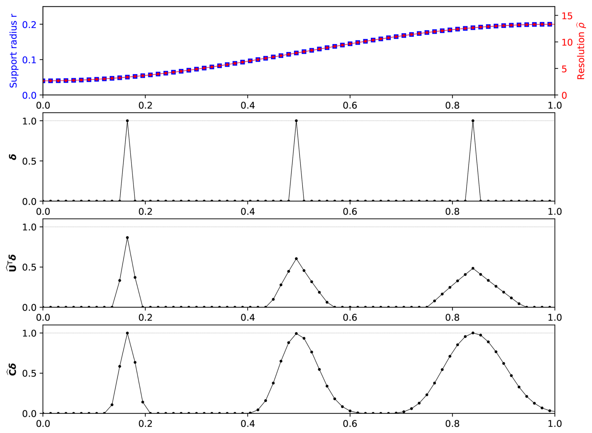
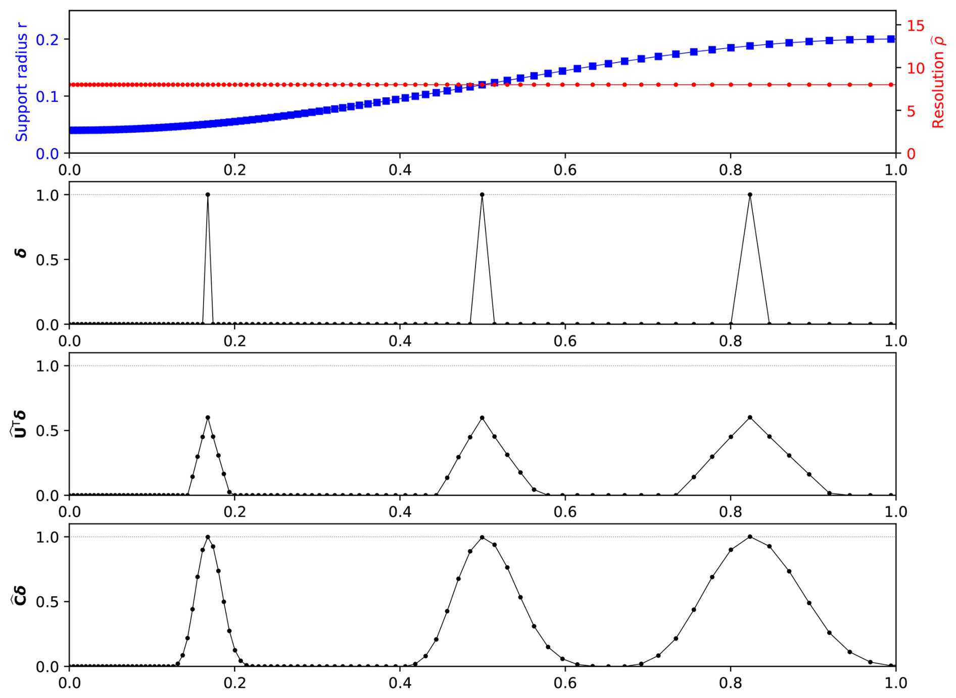
The correlation operator can also can be made inhomogeneous by using a locally varying support radius r or support tensor D. If the subgrid is kept regular, the sharpness of the correlation operator becomes inhomogeneous as well, as illustrated by Fig. 5. For the left-hand side impulse of Fig. 5, where the support radius r is small, the local correlation resolution $\widehat{\mathit{\rho }}$ is lower than 5, whereas it is larger than 10 for the right-side impulse where the support radius r is large. To enforce a homogeneous resolution $\widehat{\mathit{\rho }}=r/\widehat{\mathit{\gamma }}$ when the support radius r is locally varying, the only solution is to introduce a locally varying cell size $\widehat{\mathit{\gamma }}$ following the same pattern. Figure 6 shows such a case: the cell size is smaller on the left-hand side where r is small, and larger on the right-hand side where r is large. Thus, the sharpness of the correlation function is homogeneous, whatever the local support radius. It should be noted that the internal normalization N^′ becomes inhomogeneous for an inhomogeneous correlation resolution $\widehat{\mathit{\rho }}$, but tends to be homogeneous when the cell size is adjusted to keep a homogeneous $\widehat{\mathit{\rho }}$ (not shown in figures).

Figure 5 Same as Fig. 2 with an inhomogeneous support radius r.

Figure 6 Same as Fig. 5 with an inhomogeneous cell size $\widehat{\mathit{\gamma }}$.

3 Practical implementation

The NICAS method description in the previous section leaves many options open for the practical implementation. This section details some of the constraints and choices that seem appropriate for an efficient parallel implementation, suitable for the large grids of geophysical models.

3.1 Splitting horizontal and vertical directions

In theory, the normalized distance d_ij defined in Eqs. (5) and (6) could be fully tridimensional. However, in stratified fluids like the atmosphere or the ocean, it makes sense to split the normalized distance into horizontal and vertical components. As a consequence, the tensor formulation of Eq. (6) is always used in practice, but with zero cross-components between the horizontal and the vertical directions:

$$\begin{array}{}\text{(7)}& \mathbf{D}=\left(\begin{array}{lll}{D}_{\mathrm{1}}& D_{\mathrm{off}}& \mathrm{0}\\ D_{\mathrm{off}}& D_{\mathrm{2}}& \mathrm{0}\\ \mathrm{0}& \mathrm{0}& r_{\mathrm{v}}^{\mathrm{2}}\end{array}\right)\end{array}$$

where D₁, D₂ and D_off are the horizontal support tensor components, and r_v is the vertical support radius. In the horizontally isotropic case: $D_{\mathrm{1}}=D_{\mathrm{2}}=r_{\mathrm{h}}^{\mathrm{2}}$ and D_off=0, where r_h is the horizontal support radius. In the horizontally anisotropic case, Eq. (14) of Ménétrier et al. (2014) defines an equivalent horizontal support radius r_h associated with the horizontal part of the support tensor. r_h is chosen so that the area of the ellipse defined by horizontal support tensor is equal to the area of the circle of radius r_h:

$$\begin{array}{}\text{(8)}& r_{\mathrm{h}}={\left(D_{\mathrm{1}}{D}_{\mathrm{2}}-D_{\mathrm{off}}^{\mathrm{2}}\right)}^{\mathrm{1}/\mathrm{4}}.\end{array}$$

This equivalent support radius r_h will be useful to generate the adaptive horizontal subgrid.

Theoretically, $\widehat{\mathcal{G}}$ could be any tridimensional structured or unstructured subgrid. However, it is also relevant here to separate the vertical and horizontal directions, introducing an intermediate grid $\stackrel{\mathrm{̃}}{\mathcal{G}}$ as illustrated on Fig. 7:

• First, a vertical sub-sampling of 𝒢 is performed, based on the vertical support radius r_v and the resolution $\widehat{\mathit{\rho }}$: only a subset of the levels of the 𝒢 are kept to define the intermediate grid $\stackrel{\mathrm{̃}}{\mathcal{G}}$.

• Second, a horizontal subgrid is generated for each level of $\stackrel{\mathrm{̃}}{\mathcal{G}}$ depending on the horizontal support radius r_h (or its equivalent in the anisotropic case) and the resolution $\widehat{\mathit{\rho }}$, in order to build $\widehat{\mathcal{G}}$.

With such a subgrid construction process, the interpolation S from $\widehat{\mathcal{G}}$ to 𝒢 is efficiently performed in two steps: horizontally first to go from $\widehat{\mathcal{G}}$ to $\stackrel{\mathrm{̃}}{\mathcal{G}}$, and then vertically to go $\stackrel{\mathrm{̃}}{\mathcal{G}}$ to 𝒢.

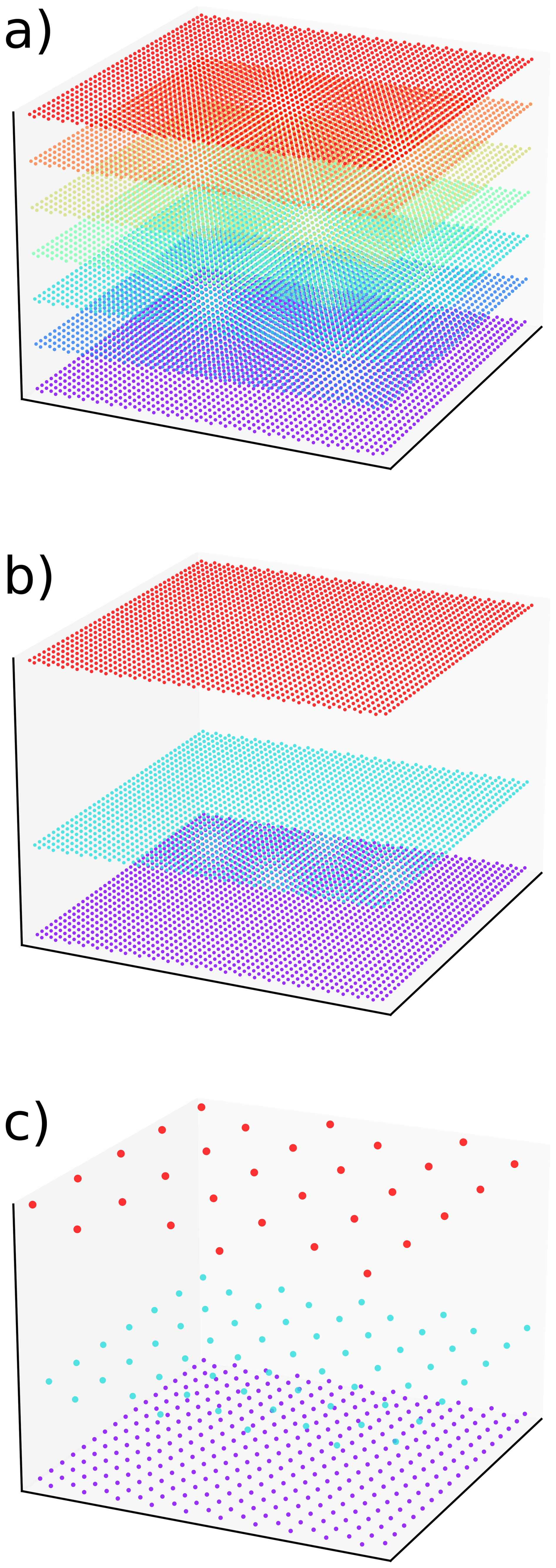
Figure 7 Example of definition of $\stackrel{\mathrm{̃}}{\mathcal{G}}$ and $\widehat{\mathcal{G}}$ from 𝒢 for a simplified case where the horizontal and vertical support radii r_h and r_v are both horizontally homogeneous and vertically increasing. (a) Full grid 𝒢, (b) intermediate grid   $\stackrel{\mathrm{̃}}{\mathcal{G}}$ and (c) subgrid $\widehat{\mathcal{G}}$. See text for details.

While the obvious choice for the horizontal distance measure on the sphere is the great-circle distance, the choice of vertical coordinate is completely free in NICAS. Any vertical coordinate field provided on 𝒢 can be used, as long as the vertical support radius r_v has the same unit as the provided coordinate. This feature is very convenient for modeling vertically coupled correlations between Earth components, like atmosphere and ocean.

3.2 Horizontal subgrid generation

Different strategies are available to generate the horizontal subgrid at each selected level of the intermediate grid $\stackrel{\mathrm{̃}}{\mathcal{G}}$:

• a.

  If the local correlation radius r is homogeneous, a regular subgrid with a known (quasi-)homogeneous resolution is relevant. For a global domain on the sphere, an octahedral Gaussian grid (Malardel et al., 2016) is a good choice. Even if its cell size is slightly inhomogeneous (larger at mid-latitudes, smaller at the poles), it is possible to precisely select its truncation to obtain the desired subgrid cell size $\widehat{\mathit{\gamma }}$ on average. For a regional domain, a subgrid made of equilateral triangles on the projection plane is a good candidate.

• b.

  A random sampling can yield a more homogeneous subgrid, especially if it has a blue noise distribution (also known as Poisson disk sampling) that avoids clusters of sampled points. The Bridson's algorithm (Bridson, 2007) is a fast and reliable method to generate such a sampling in arbitrary dimensions, and it can be adapted on the sphere with a minor modification of the annulus random sampling step.

• c.

  If the local correlation radius r is inhomogeneous, the Bridson's algorithm can also be modified to take into account the variations of the Poisson disk radius.

Figure 8 shows an example of each of these three strategies for a global domain. The Bridson's algorithm provides a more homogeneous sampling in case (b) than the octahedral Gaussian grid of case (a), and the local sampling density is consistently adjusted to the varying local support radius provided by the user in case (c).

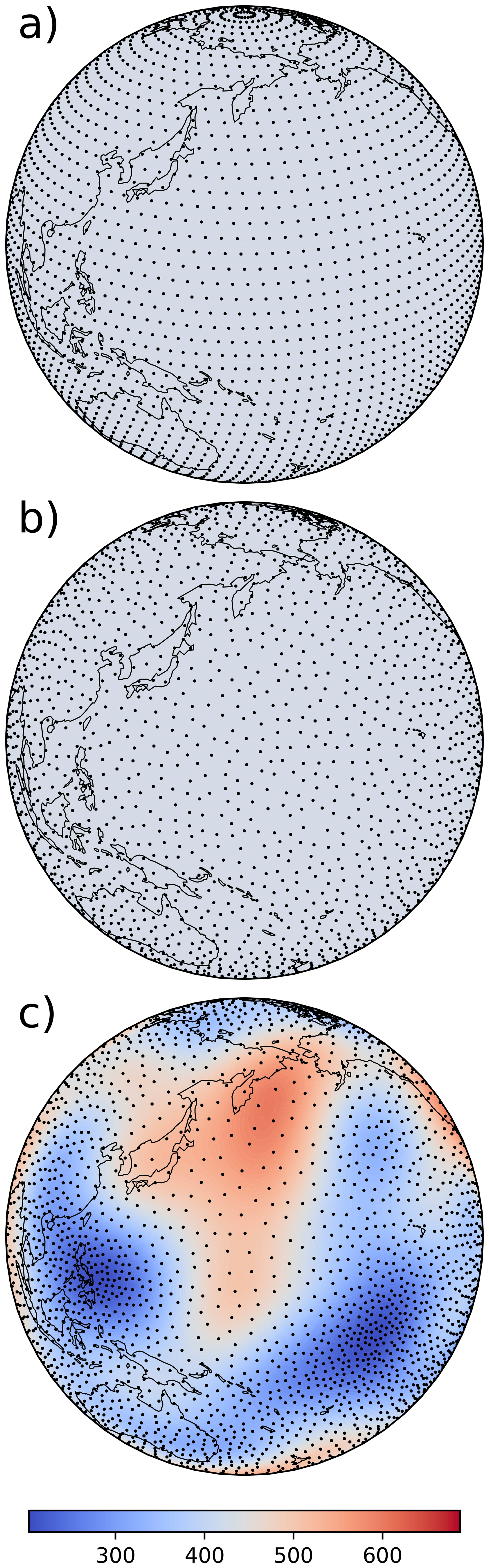
Figure 8 Sampling strategies: (a) octahedral Gaussian grid for a homogeneous radius r; (b) Bridson's algorithm for a homogeneous radius r; (c) Bridson's algorithm for an inhomogeneous radius r. Typical subgrid cell size $\widehat{\mathit{\gamma }}$ (in km) is given by the color scale.

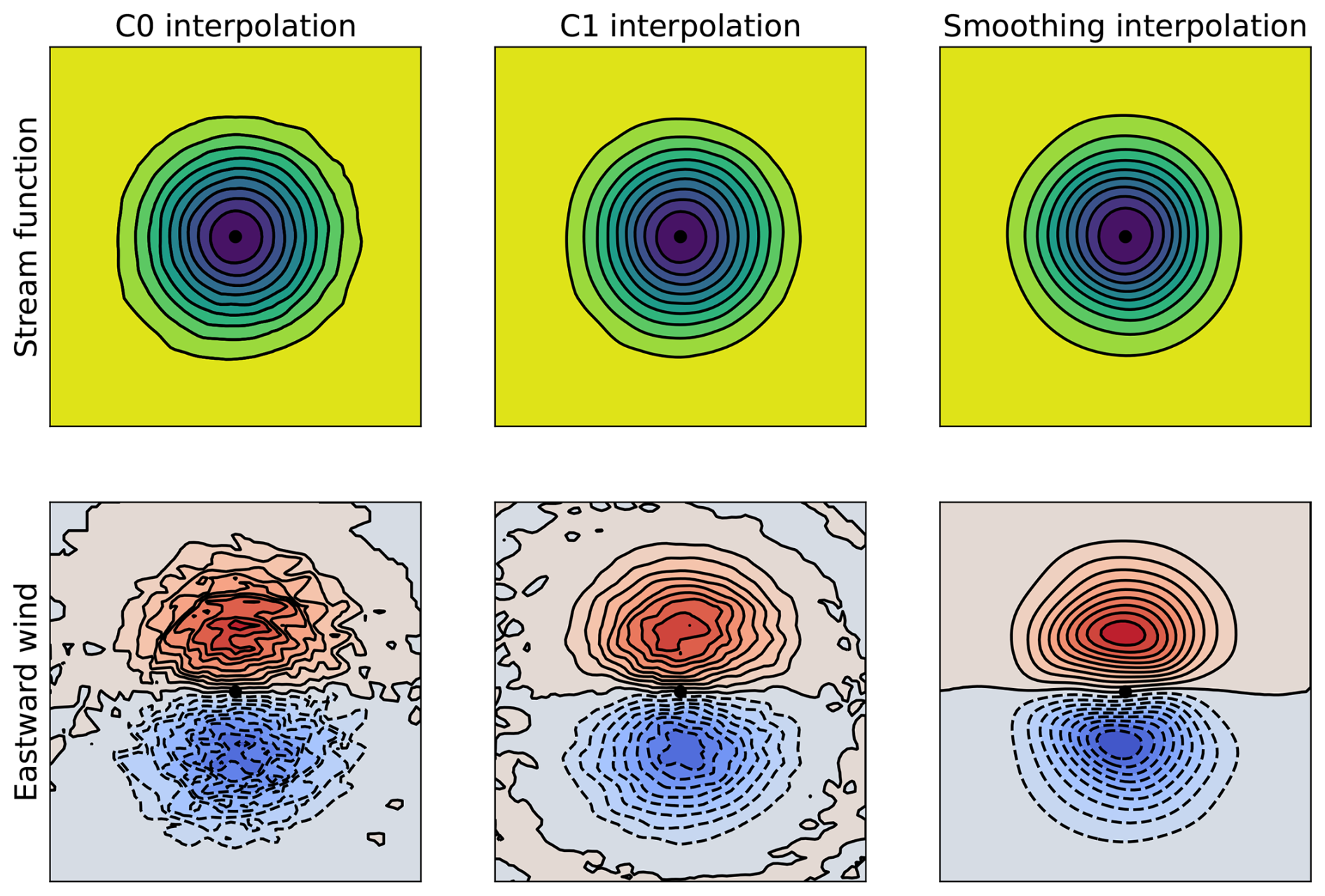
Figure 9 Top panels: correlation function (stream function) obtained for an initial impulse at the black dot location, with 𝒞⁰, 𝒞¹ and smoothing interpolations from left to right, respectively. Bottom panels: corresponding meridional derivative (eastward wind). Units are arbitrary, but color scales are similar for each row.

3.3 Interpolation choice

The implementation of the interpolation S in Eq. (1) should depend on the usage of the NICAS method. For the vertical direction, a linear interpolation seems to be sufficient, even if a higher order one could be easily implemented. For the horizontal direction, assuming that $\widehat{\mathcal{G}}$ is unstructured, the simplest option is a linear interpolation based on the Delaunay tesselation of the subgrid. However, the output field resulting from this type of interpolation is of class 𝒞⁰, which means that it is continuous but has potentially discontinuous derivatives. This discontinuity can be harmful if the derivatives of the analysis variables are important for subsequent calculations. For instance, if the analysis wind variables are the stream function φ and the velocity potential ψ, the physical wind components u and v based on the derivatives of φ and ψ will be discontinuous, as shown in the left panel of Fig. 9.

A possible solution is to introduce a more advanced interpolation producing fields of class 𝒞¹, with continuous first-order derivatives. The SSRFPACK library (Renka, 1997) implements such an interpolation, using local estimates of the function gradient at each subgrid point (Renka et al., 1984). Even if this interpolation significantly improves the continuity of u and v in the central panel of Fig. 9, the results are still noisy because of the errors in the local gradient estimation procedure provided with SSRFPACK.

Since the convolution operator $\widehat{\mathbf{C}}$ on $\widehat{\mathcal{G}}$ is a smoother, there is actually no need for an accurate interpolation between $\widehat{\mathcal{G}}$ and 𝒢. A smoothing interpolation could ensure smooth results on 𝒢. Its local smoothing support radius should be defined as a fraction of the horizontal correlation support radius r_h, for consistency. However, this secondary smoothing would increase the initially intended smoothing on 𝒢. To alleviate this issue, an empirical reduction factor can be applied on the horizontal support radius (or tensor), which in turn increases the size of $\widehat{\mathcal{G}}$ and the overall cost. So this option is slightly more costly, but it provides very clean results as shown on the right panel of Fig. 9. While the differences seem minor between the correlation functions themselves for the three different interpolations (top row), the impact on the derivative can very large (bottom row).

3.4 Normalization calculation

One significant advantage of the NICAS method over other existing methods is its exact normalization (C_ii=1). Once the square-root of the correlation operator on $\widehat{\mathcal{G}}$ (i.e. $\widehat{\mathbf{U}}$) and the interpolation from $\widehat{\mathcal{G}}$ to 𝒢 (i.e. S) are defined, the normalization operator N is computed as the inverse of the square-root of the diagonal of $\mathbf{S}\widehat{\mathbf{U}}{\left(\widehat{\mathbf{U}}\mathbf{S}\right)}^{\mathrm{T}}$. Defining the vector δ_i∈ℝⁿ as a vector of zeros, except for a value one at the ith position, N_ii can be computed as:

$$\begin{array}{}\text{(9)}& \begin{array}{rl}{N}_{ii}& ={\left({\mathit{\delta }}_i^{\mathrm{T}}\mathbf{S}\widehat{\mathbf{U}}{\left(\widehat{\mathbf{U}}\mathbf{S}\right)}^{\mathrm{T}}{\mathit{\delta }}_i\right)}^{-\mathrm{1}/\mathrm{2}}\\ & ={〈{\left(\widehat{\mathbf{U}}\mathbf{S}\right)}^{\mathrm{T}}{\mathit{\delta }}_i,{\left(\widehat{\mathbf{U}}\mathbf{S}\right)}^{\mathrm{T}}{\mathit{\delta }}_i〉}^{-\mathrm{1}/\mathrm{2}}\\ & ={∥{\left(\widehat{\mathbf{U}}\mathbf{S}\right)}^{\mathrm{T}}{\mathit{\delta }}_i∥}_{\mathrm{2}}^{-\mathrm{1}}\end{array}\end{array}$$

where 〈⋅〉 denotes a canonical inner product and $\parallel \cdot {\parallel }_{\mathrm{2}}$ the corresponding L² norm. Thus, N_ii can be exactly computed using Algorithm 1. This operation involves a lot of bookkeeping and it can be costly, but a parallel implementation is straightforward and significantly reduces this cost.

Algorithm 1 Normalization computation

for each point p_i in 𝒢 do

Initialize v_i=0.

Prepare the list ℒ_i of all the points p_ij of $\widehat{\mathcal{G}}$ involved in the interpolation to point p_i, together with their respective interpolation weights w_ij.

for each couple (p_ij,w_ij) in ℒ_i do

Prepare the list ℒ_ij of all the points p_ijk of $\widehat{\mathcal{G}}$ involved in the correlation square-root at point p_ij, associated with their respective square-root convolution weights w_ijk.

Sum the contributions of all the points p_ijk on v_i:

$$\begin{array}{}\text{(10)}& {\displaystyle }{v}_i\leftarrow v_i+w_{ij}\sum _{{\mathcal{L}}_{ij}}{w}_{ijk}\end{array}$$

end for

Compute the normalization coefficient: $N_{ii}=v_i^{-\mathrm{1}/\mathrm{2}}$

end for

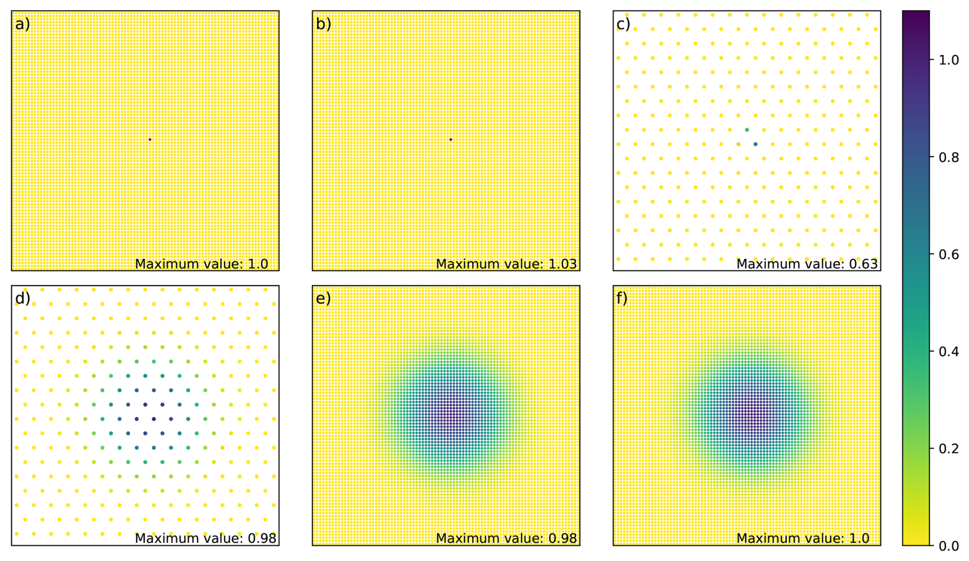
Figure 10 NICAS steps for an isotropic correlation function: δ_i (a), N^Tδ_i (b), S^TN^Tδ_i (c), $\widehat{\mathbf{C}}{\mathbf{S}}^{\mathrm{T}}{\mathbf{N}}^{\mathrm{T}}{\mathit{\delta }}_i$ (d), $\mathbf{S}\widehat{\mathbf{C}}{\mathbf{S}}^{\mathrm{T}}{\mathbf{N}}^{\mathrm{T}}{\mathit{\delta }}_i$ (e) and $\mathbf{NS}\widehat{\mathbf{C}}{\mathbf{S}}^{\mathrm{T}}{\mathbf{N}}^{\mathrm{T}}{\mathit{\delta }}_i$ (f). The exact maximum value is indicated at the bottom right for each panel.

3.5 Steps illustration

To illustrate how the NICAS method works in practice, the operator C of Eq. (1) is applied to an impulse vector δ_i, and the result at each step is displayed. Figure 10 shows these steps for an isotropic correlation function, and Fig. 11 for an anisotropic correlation function with a land/sea mask. The normalization N ensures that the correlation function maximum is equal to one at the end of the last step, even if the impulse on 𝒢 is not collocated with a point $\widehat{\mathcal{G}}$. To take the land/sea mask into account in Fig. 11:

• all the masked points (land mask) are removed from both 𝒢 and $\widehat{\mathcal{G}}$,

• for all the correlation and interpolation operations, the operation is removed if the segment between the two points involved in the operation crosses a segment of the masked area boundary.

This last check can be costly, depending on the mask resolution. However, it is possible to split the NICAS usage into two successive steps:

• A setup step, where (i) the subgrid is generated, (ii) the interpolation from the subgrid to the full grid is defined, (iii) the convolution on the subgrid is computed, and (iv) the normalization of the whole operator is estimated. Most of the computational cost occurs during this phase, including the additional cost associated with advanced features such as inhomogenous, anisotropic, or boundary-aware correlation functions. The resulting operators are generally stored into dedicated files (NetCDF format), either one file per MPI task or in a common global file, for a future use. If a common global file is read in a subsequent execution, a data redistribution is needed, which comes with a extra communication cost.

• An application step, where the NICAS operator is applied on fields. This application includes computation and communication sub-steps for both the interpolation and the convolution applications, and the multiplication with the normalization field.

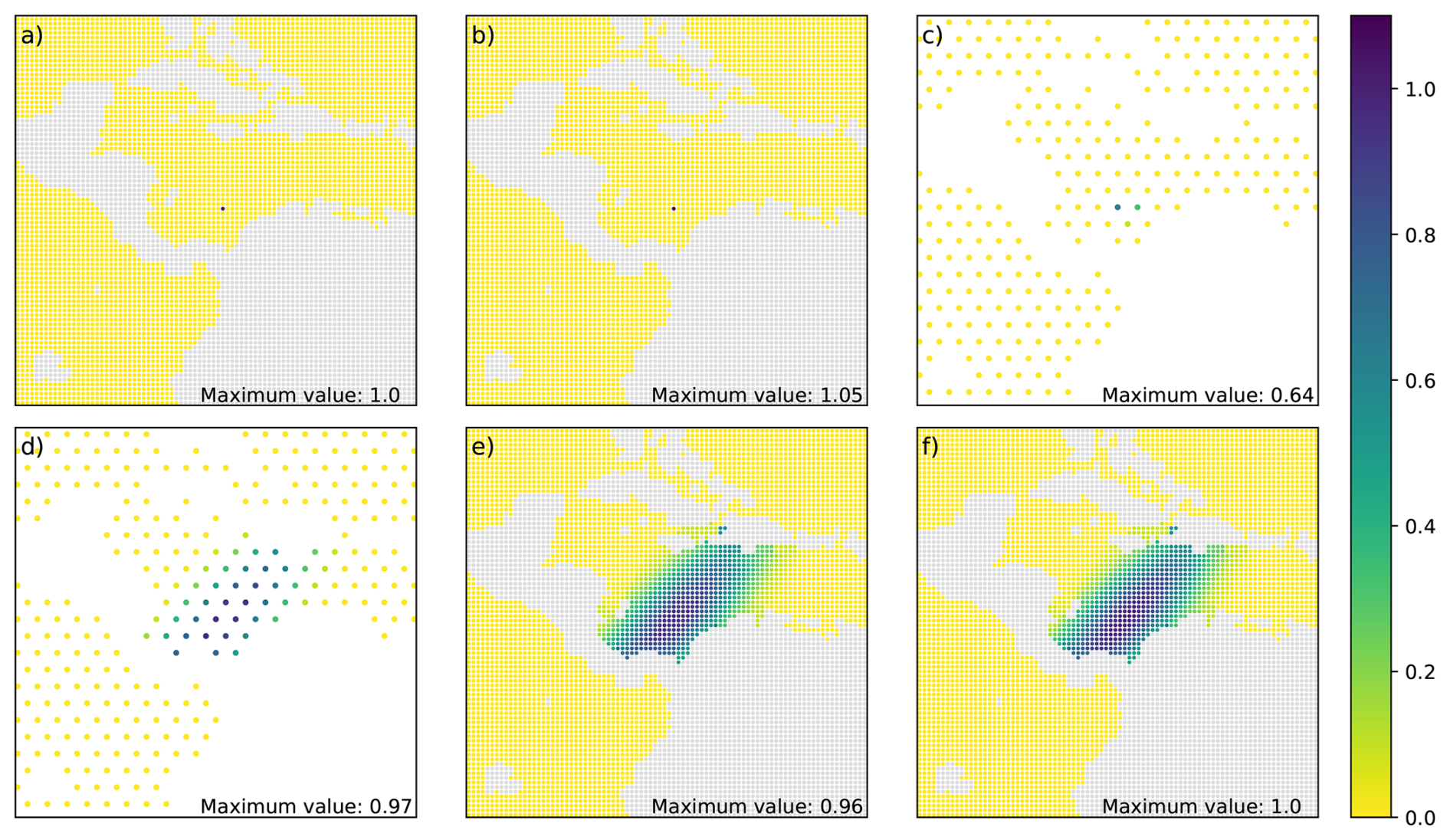
Figure 11 Same as Fig. 10 for an anisotropic correlation function with a land/sea mask.

4 Computational cost and scalability

Evaluating the computational cost of a new method is a complex task because it depends on many parameters, on the parallel configuration, on the hardware, etc. The goal of this section is to give a broad overview of how the cost of the NICAS method is impacted by key parameters, how the method scales, and where speed up gains could be obtained in the future.

4.1 Experimental setup

All the experiments in this section are performed on a single horizontal level, because the vertical aspect of NICAS has little impact on performances. The grid 𝒢 is an octahedral Gaussian grid at truncation TCo600 (n=1 461 600, γ∼16.5 km at the equator) and is the same for all the experiments. To obtain a given correlation resolution ρ on 𝒢, the correlation support radius r is given by r=γρ. Then, to obtain a given correlation resolution $\widehat{\mathit{\rho }}$ on $\widehat{G}$, the subgrid cell size is set as $\widehat{\mathit{\gamma }}=r/\widehat{\mathit{\rho }}=\mathit{\gamma }\mathit{\rho }/\widehat{\mathit{\rho }}$. As a consequence, the subgrid size is $\widehat{n}\propto {\widehat{\mathit{\gamma }}}^{-\mathrm{2}}\propto {\left(\widehat{\mathit{\rho }}/\mathit{\rho }\right)}^{\mathrm{2}}$. Since r is homogeneous, $\widehat{G}$ is defined as a regular octahedral Gaussian grid with the appropriate truncation to fit the target subgrid cell size $\widehat{\mathit{\gamma }}$, unless stated otherwise. The interpolation method is the simplest 𝒞⁰ linear interpolation based on a Delaunay tesselation of $\widehat{G}$, unless stated otherwise. All the experiments are performed on a dedicated compute node of the BullSequana XH2000 HPC of ECMWF. The results are the average elapsed timings of 10 executions for the setup step (where the NICAS operators are computed) and 100 executions for the application step (where they are applied to a vector).

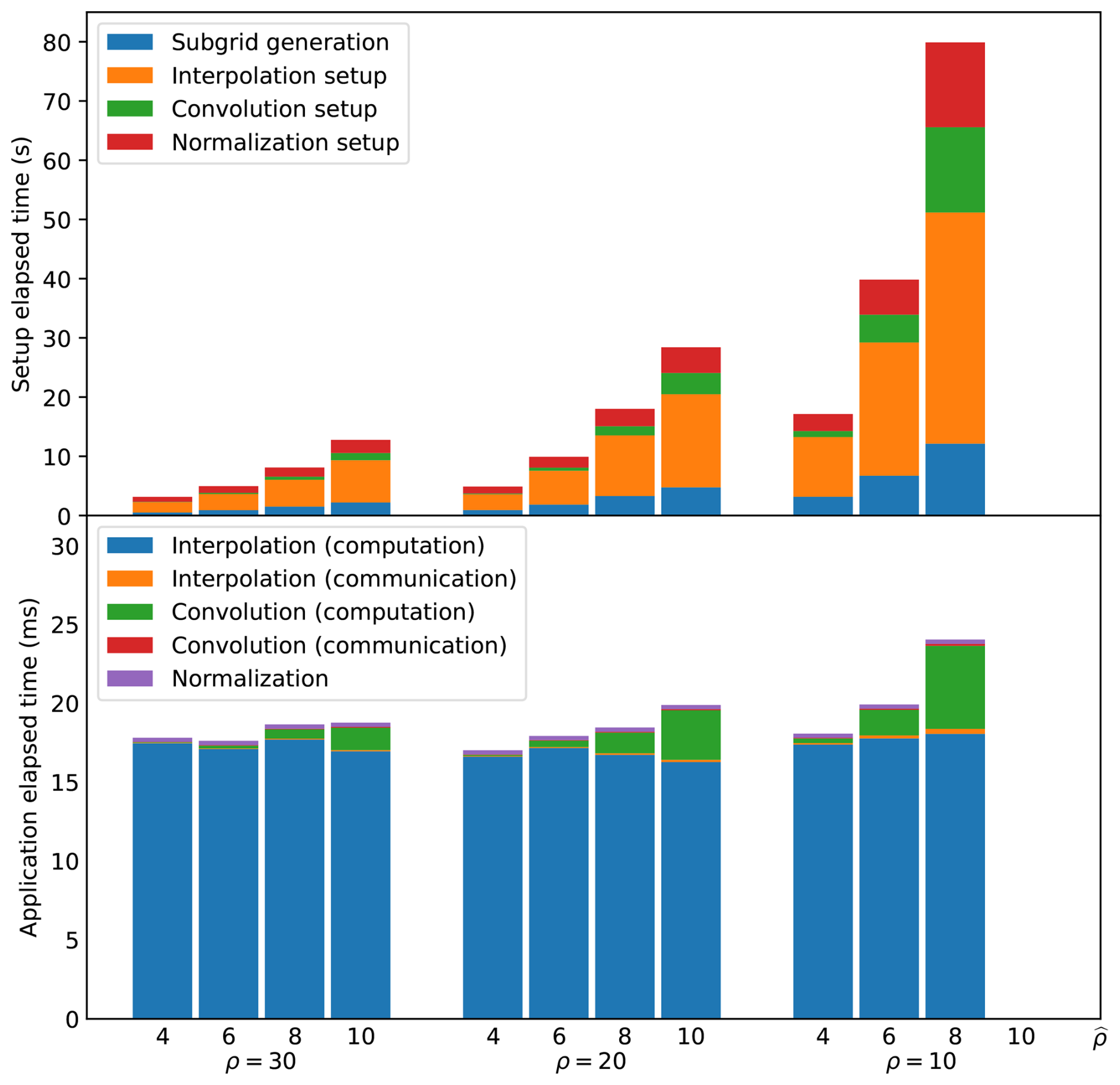
Figure 12 Timings for different combinations of the correlation resolutions ρ and $\widehat{\mathit{\rho }}$, for the setup step (top panel) and the application step (bottom panel).

4.2 Correlation resolution

As explained in Sect. 2.1, the correlation resolutions ρ and $\widehat{\mathit{\rho }}$ have a major impact on the cost of the NICAS method, and they can make it very competitive or very costly. An order-of-magnitude analysis can be conducted for the different steps of the NICAS method:

1. For the setup step:

   • The cost of the subgrid generation is mostly due to the assignment of each subgrid point to a given MPI task, depending on its location. This cost increases linearly with the subgrid size $\widehat{n}\propto {\left(\widehat{\mathit{\rho }}/\mathit{\rho }\right)}^{\mathrm{2}}$.

   • The cost of the interpolation setup increase with n, kept constant here, and with $\widehat{n}\propto {\left(\widehat{\mathit{\rho }}/\mathit{\rho }\right)}^{\mathrm{2}}$ for the generation of the tesselation to compute the interpolation weights.

   • The cost of the convolution setup increases with the subgrid size $\widehat{n}$ multiplied by the number of points within a radius r, which is ${\widehat{n}}_c\propto r^{\mathrm{2}}\widehat{n}\propto {\widehat{\mathit{\rho }}}^{\mathrm{2}}$. So the total cost should be proportional to ${\widehat{\mathit{\rho }}}^{\mathrm{4}}/{\mathit{\rho }}^{\mathrm{2}}$.

   • The cost of the normalization setup is mostly due to the inversion of indices list, which increases with $\widehat{n}\propto {\left(\widehat{\mathit{\rho }}/\mathit{\rho }\right)}^{\mathrm{2}}$.

2. For the application step:

   • The cost of the normalization and the interpolation applications is proportional to n (constant).

   • The cost of the convolution application is proportional to $\widehat{n}{\widehat{n}}_c\propto {\widehat{\mathit{\rho }}}^{\mathrm{4}}/{\mathit{\rho }}^{\mathrm{2}}$.

Figure 12 provides a confirmation of this analysis, for experiments on 32 MPI tasks, with a few more interesting points. First, the setup step is several orders of magnitude more expensive than the application step. In the application step, the cost of communications is negligible (only local halo exchange), the cost of normalization is also very small, and the cost of convolution is significantly smaller than the cost of interpolation. This was the fundamental idea of the NICAS method design detailed in Sect. 2.1: making the whole cost dominated by the interpolation, which depends on the size n of 𝒢 and the type of interpolation, independently from the convolution itself.

4.3 Interpolation impact

Figure 13 shows the impact of the interpolation type alone, the other parameters being held constant (32 MPI tasks, ρ=20, $\widehat{\mathit{\rho }}=\mathrm{8}$). Among the three interpolations tested here, the 𝒞⁰ linear interpolation based on a Delaunay tesselation is of course the cheapest. The 𝒞¹ upgrade, which requires the estimation of gradients at the vertices of the interpolation triangle is slightly more expensive. With the smoothing interpolation, needed to get continuous derivatives, the correlation support radius r needs to be artificially decreased in order to compensate for the “double-smoothing” in both the convolution and the interpolation operators. In the current experiment, r needed to be multiplied by a factor 0.7 to obtain the same total correlation radius. Thus, the size $\widehat{n}$ of the subgrid was multiplied by approximately ${\mathrm{0.7}}^{-\mathrm{2}}\simeq \mathrm{2}$, which explains the amplitude of the cost increase for both the setup and the application steps.

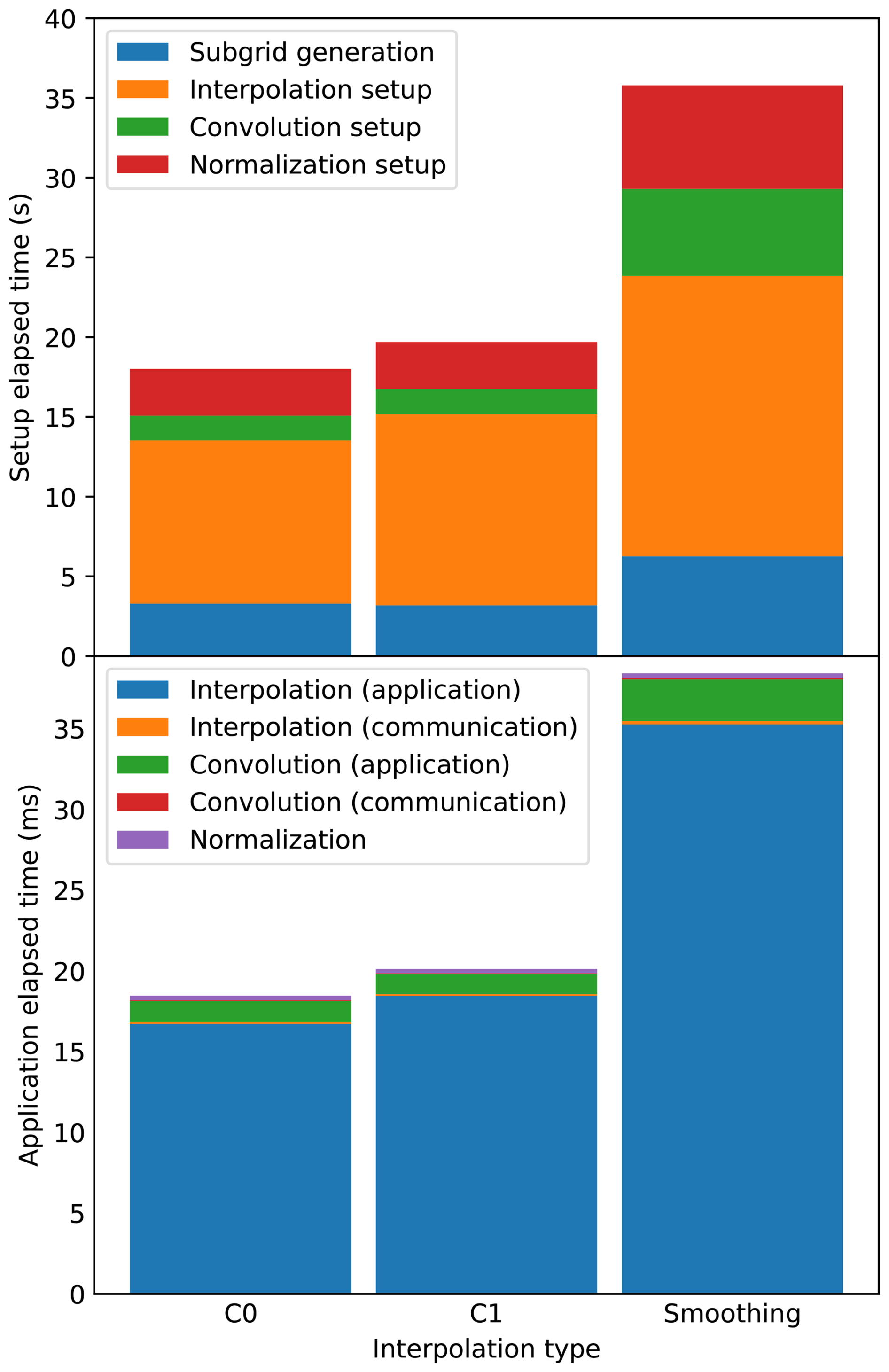
Figure 13 Timings for different interpolation types, for the setup step (top panel) and the application step (bottom panel).

4.4 Scalability

To evaluate the NICAS method scalability, the same experiment (ρ=20, $\widehat{\mathit{\rho }}=\mathrm{8}$) is run with either 16, 32, 64 or 128 MPI tasks. Since a single HPC node is always used, the cost of communications might be underestimated here. Indeed, it would probably be larger on several nodes because of slower inter-nodes communications. For sake of comparison, a “perfect scalability” curve is computed by extrapolating the timing of the case with the lowest number of MPI tasks and dividing this timing by a factor 2 each time the number of MPI tasks increases by a factor 2.

Figure 14 shows that the setup step does not scale perfectly, mostly because of the interpolation setup and the subgrid generation. Indeed, the tesselation algorithm (STRIPACK) that accounts for an important part of the interpolation setup is not parallel. Similarly, the assignment of each subgrid point to a given MPI task in the subgrid generation is not parallel neither. However, the application step scales very well and closely follows the “perfect scalability” curve. This is a real important feature of the NICAS method.

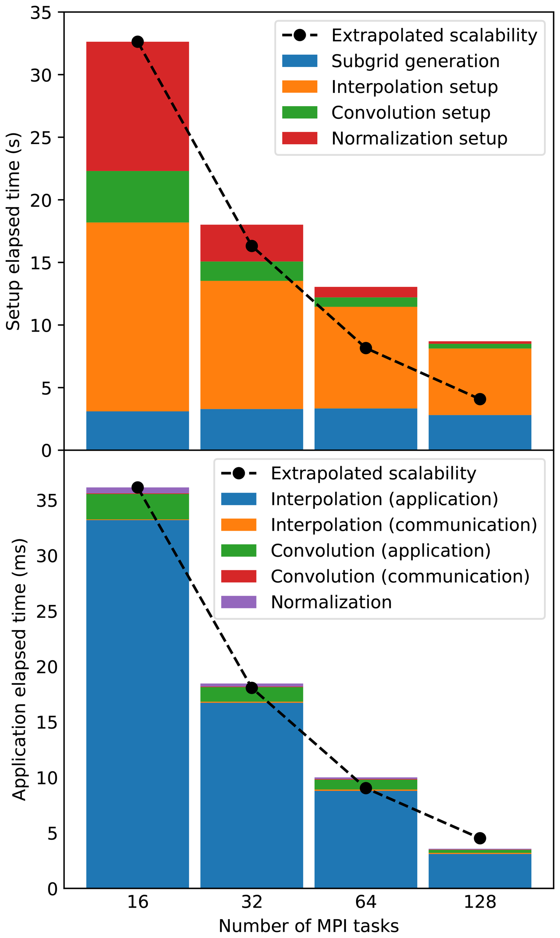
Figure 14 Timings for different numbers of MPI tasks, for the setup step (top panel) and the application step (bottom panel). The dashed black line indicates a perfect scalability extrapolated from the lowest number of MPI tasks.

As noted before, the setup step is several orders of magnitude more expensive than the application step and it does not scale as well, even though most of the development efforts have been (and still are) devoted to its acceleration. But it is not a blocking issue because:

• The setup step can be run before the time critical path of the data assimilation process, i.e. as a preparation step before all the observations are available.

• Once the NICAS operators are computed and stored in dedicated files as sparse operators (indices and weights), they can be read efficiently in a following run and the setup step becomes much faster.

• The most important goal is to get the application step fast and scalable, because it is run in the time critical path, and it needs to be run many times during the minimization, as mentioned in the introduction.

5 Discussion

The NICAS method presented here is only one new option among many existing algorithms to apply a correlation operator on a vector in a variational data assimilation context. Here is a non-exhaustive overview of the most commonly used methods:

• Explicit convolution: this brute-force method would require the storage and application of huge matrices, which is absolutely not possible in practice for large systems.

• Spectral-based methods (Parrish and Derber, 1992; Courtier et al., 1998): the correlation operator is assumed to be diagonal in a basis of orthogonal functions, built from spherical harmonics for the whole sphere or Fourier harmonics for rectangular regional domains. Thanks to the optimized implementations of spectral transforms, this is a very fast method, whose speed is independent from the correlation support radius. It is also perfectly normalized. But it has several limitations: the resulting correlation functions are homogeneous and isotropic, they cannot take complex boundaries into account. Besides, the spectral transforms require specific regular grids and need global communications among MPI tasks.

• Wavelets-based methods (Fisher, 2003): same approach as the spectral-based method, but using a basis of wavelet functions to relax the homogeneity assumption.

• Diffusion-based methods (Weaver and Courtier, 2001): the application of a correlation operator to a vector can be seen as the result of a diffusion process with an extra normalization step. This process can take complex boundaries into account, and can produce inhomogeneous and anisotropic functions. It can even be extended to a generalized diffusion equation including a polynomial of the Laplacian operator, and produce negative lobes. In an explicit formulation, solving such equations only requires local halo communications, but a lot of iterations can be needed to maintain the numerical accuracy and stability, especially for large correlation support radii. With the implicit formulation (Mirouze and Weaver, 2010), the iterative solving is more stable but requires global communications (to compute dot products), although this limitation can be partially avoided with the Chebyshev iteration method described in Weaver et al. (2018). Normalization is also a major issue because the analytical estimates are not accurate (Weaver et al., 2020). Recent attempts with deep-learning approaches show promising ways for solving this issue (Skrunes et al., 2023).

• Recursive filters (Purser et al., 2003a, b): in a 1D framework, implicit diffusion can be implemented as a recursive filter, which is fast and stable but shares the normalization issue of diffusion-based methods. Applied successively in all directions, recursive filters can generate multi-dimensional correlation functions that are inhomogeneous and potentially anisotropic (Liu et al., 2007). Obviously, this method requires regular grids. The usual parallelization along rows, columns and levels does not scale optimally and requires global communications.

• Beta filters (Purser et al., 2022): this explicit multi-grid implementation of compactly supported beta distributions could be seen as the closest relative of the NICAS method. It shares its idea of reducing the grid resolution and using compactly supported functions, but differs in many aspects. The beta filters can use multiple subgrids instead of one for the NICAS method. However for the beta filters, these subgrids are regular subdivisions of the initial grid, and are not adaptive with respect to the local length-scale. Also, the beta filters are not perfectly normalized, contrary to the NICAS method.

It would be unfair to conclude that one of these methods is better than all the others. Each one is well-adapted to specific applications and configurations. The NICAS method is a particularly relevant candidate for: unstructured grids, domains with complex boundaries, inhomogeneous and anisotropic correlation functions, large correlation support radii. Hybridization of these methods could also be a promising avenue, for instance to obtain a peaked correlation function from a combination of Gaussian-like functions as in Fig. 4: the largest scales could be handled by NICAS and the smallest ones by a diffusion method.

6 Conclusions

This article has described the Normalized Interpolated Convolution on an Adaptive Subgrid (NICAS) method, a new way of applying a correlation operator to a vector for high-dimensional systems. This approach is not based on a theoretical breakthrough, but it relies on a precise order-of-magnitude analysis of the computational costs, followed by a careful implementation. Among the interesting features of the method, we can cite:

• the fine control of the accuracy/cost trade-off, with the subgrid resolution parameter,

• the ability to efficiently represent inhomogeneous correlation functions, with the adaptive subgrid,

• the capacity to handle anisotropic functions and complex boundaries, with the explicit convolution specification,

• the exact normalization, with the explicit knowledge of all operations.

We have shown in simplified cases that the scalability of the method behaved as expected, with a very good scalability for the application step, while some parts of the setup step are not parallelized yet. Since the real added value of the NICAS method lies in its practical implementation, this is where improvements could be made. For instance, the horizontal subgrid generation with the Bridson's algorithm could be parallelized, as well as the Delaunay tesselation generation needed for the 𝒞⁰ and 𝒞¹ interpolations.

The NICAS method has been designed with variational data assimilation in mind, but it can also be useful to generate random fields with specific spatial structures. These fields are needed, for instance, as perturbations in various stochastic methods for ensemble forecasting.

The BUMP block of the SABER library where NICAS is implemented also contains specific tools dedicated to the estimation of correlation and localization length-scales from an ensemble. These diagnostics are specifically designed to be consistent with the NICAS method and to provide horizontal and vertical support radius fields, support tensor fields for the anisotropic case, and amplitude fields for the multi-components case. This part of the code was beyond the scope of the present article and will be the main topic of a future publication.