From reanalysis to climatology: deep learning reconstruction of tropical cyclogenesis in the western North Pacific

Tropical cyclogenesis (TCG) climatology is the key to understanding regional weather extremes and long-term risk, yet their large-scale environmental drivers remain difficult to characterize from observations or traditional physical-based modeling. In this study, we present a deep learning (DL) framework based on an 18-layer residual convolutional neural network (TCG-Net) to reconstruct TCG climatology in the western North Pacific (WNP) basin from climate reanalysis data. The framework addresses two tasks (1) the Past Domain (PD) task that predicts when TCG occurs in the WNP within the next 48 h, and (2) the Dynamic Domain (DD) task that predicts the spatial distribution of TCG at a given date and time. For each task, different labeling strategies are employed to generate negative samples that can help maximize the distinction between TCG and non-TCG conditions. To enhance the model's capability in handling the rarity of TCG data, temporal feature enrichment is further used to incorporate environmental information from the preceding 6 h time steps, which helps improve the representation of each training task. In addition, random under-sampling is applied with class weighting to address the severe imbalance caused by large numbers of negative TCG samples under these labeling strategies. Using NASA's Modern-Era Retrospective analysis for Research and Applications Version 2 (MERRA-2) with a training period from 1980–2016 and a test set from 2017–2022, we show that TCG-Net achieves an overall F₁-score of 0.39 for the PD task and 0.33 for the DD task. In the PD task, feature selection experiments reveal that only a subset of environmental variables is required for robust performance, consistent with prior physical studies. In contrast, for the DD task, full-feature models perform better, likely due to their ability to exploit unknown or latent feature interactions. Both tasks reproduce key characteristics of the observed seasonality and spatial TCG distribution when evaluated against the best-track dataset. These results demonstrate that DL-based reconstructions, when coupled with task-specific labeling, temporal enrichment, and imbalance-aware training, can complement physics-based models and vortex-tracking algorithms and provide an efficient pathway for downscaling or projecting TCG climatology from coarse-resolution climate model outputs.

1 Introduction

The western North Pacific (WNP) basin has been well-documented to be the most active area of tropical cyclone (TC) activities (Kossin et al., 2016; Peduzzi et al., 2012; Tran-Quang et al., 2020). With favorable conditions for TC formation (also known as tropical cyclogenesis, or TCG) such as warmer sea surface temperature (SST), active monsoon trough formation, or frequent convectively coupled equatorial waves, WNP produces about 25–30 TCs annually with a quarter of that affecting Vietnam coastal regions (Defforge and Merlis, 2017; Trinh et al., 2021; Thanh et al., 2020). From the climate perspective, any change in TC main characteristics such as frequency, genesis locations, or intensity is often considered to be a manifestation of climate change. Thus, developing effective methods to construct TC climatology from different climate datasets is of significant importance for studying future projections of TC climatology from climate model outputs or outlooks from global forecasting systems (e.g., Knutson et al., 1998; Walsh et al., 2007; Bengtsson et al., 2007; Lee et al., 2020; Cha et al., 2020; Camargo et al., 2023; Kieu et al., 2023).

Traditionally, creating a TC climatology from gridded climate output involves using a vortex tracking algorithm to detect TC centers. This algorithm relies on a set of TC characteristics, such as absolute vorticity, surface maximum wind, minimum central pressure, warm core, or lifetime, which are checked at each model grid point (Walsh et al., 2015; Zhao et al., 2009; Strachan et al., 2013; Camargo and Zebiak, 2002; Horn et al., 2014; Zarzycki and Ullrich, 2017; Ullrich and Zarzycki, 2017; Vu et al., 2021). While being effective for high-resolution model outputs where TC characteristics are well-captured and thus suitable for weather forecast models or well-developed TCs, vortex tracking methods face challenges with coarse-resolution climate models (>0.5°). For these coarse-resolution models or datasets, TC characteristics, especially during early formation, are often unclear (Zarzycki and Ullrich, 2017; Tien et al., 2020). Consequently, directly tracking a vortex from such outputs can lead to uncertainties in the timing and location of early TCG. This issue becomes more apparent when studying climate change aspects like shifts in TCG location or timing across different climate datasets (e.g., Tan et al., 2015; Tien et al., 2020).

The rapid advancement of machine learning (ML) techniques has opened new avenues for atmospheric research as well as operational forecasting. Given the vast amount of observational and model-generated data, weather and climate systems naturally provide a “big data” platform that are well-suited for training ML models not only for short-term weather prediction but also for capturing long-term climate variability (e.g., Schultz et al., 2021; Pathak et al., 2022; Bi et al., 2023; Lam et al., 2023; Nguyen and Kieu, 2024). In fact, many private and governmental organizations have recently developed deep learning architectures that outperform traditional physics-based models in weather forecasting, as demonstrated by Pathak et al. (2022) and Lam et al. (2023).

Among recent applications of ML to TC research, most efforts have been limited to short-term contexts such as weather forecasting, satellite retrieval, or diagnostic studies. For examples, Miller et al. (2017), Wimmers et al. (2019) developed a deep learning (DL) model with satellite data to train a convolutional neural network, which can categorize TC intensity based on different cloud patterns and satellite channels. This line of approach has been further advanced to help improve TC forecasts by integrating the tracking information and/or other reanalysis data, with some modest performance for nowcasting and diagnoses (e.g., Gao et al., 2018a; Kim et al., 2019b; Chen et al., 2020; Giffard-Roisin et al., 2020).

Specific to TCG study from climate data (Nguyen and Kieu, 2024), hereinafter NK2024, recently evaluated several DL architectures and identified promising potential for early warning of TCG events in the WNP basin. Using NCEP reanalysis data and formulating TCG detection as a classification problem, they demonstrated reasonable forecast skill of DL models, even at a coarse spatial resolution of 1°×1°. While the model’s predictive skill declines with increasing forecast lead time, their approach highlights an important capability of detecting TCG directly from climate outputs. In particular, certain DL architectures can be used to identify both the location and timing of TCG events within a given domain, which is valuable for broader applications in TCG climatology or future projections. It is important to emphasize here the distinction between predicting and detecting TCG. While long-lead TCG prediction suffers from rapidly decreasing skill due to the inherent limits of predictability in tropical dynamics, detecting TCG from coarse-resolution climate data (also known as downscaling) proves to be much more skillful and feasible. The reason is that detection relies primarily on identifying favorable environmental conditions at the time of genesis, making it a problem of climate downscaling rather than one constrained by the chaotic dynamics of the atmosphere.

Although existing ML applications for TC research show some promises, they have focused so far mostly on short-term prediction or nowcasting, rather than on TC climatology. Specifically, the use of ML for constructing TC climatology remains relatively preliminary (e.g., Scher and Messori, 2019; Wang et al., 2022; Chen and Yuan, 2024). Key challenges include how to leverage ML to diagnose climate model outputs, identify and correct model biases, or construct robust statistics of large-scale climate features. Thus, the development of ML-based techniques for downscaling of TC climatology or distributions of any other extreme events from reanalysis data is largely unexplored, yet represents an important open direction for future applications of DL for climate research.

Given the rapid advancements in DL techniques, the main objective of this study is to introduce TCG-Net, a framework for reconstructing TCG climatology from climate reanalysis datasets. Specifically, we will extract key TCG characteristics such as frequency or spatial distribution from the NASA Modern-Era Retrospective analysis for Research and Applications, Version 2 (MERRA-2), instead of forecasting TCG as in, e.g., NK2024. Our DL-derived TCG climatology can serve as an independent validation and complement to those obtained from traditional vortex tracking methods. Furthermore, any TC climatology obtained from MERRA-2 data can also be used as a reference for examining the change of TC climatology in future projections, which justifies our DL approach herein.

The rest of this work is organized as follows. In Sect. 2, details of data pre-processing and our CNN algorithms are presented. An approach to generate and label TCG binary dataset for each application will also be discussed. Section 3 presents the detailed design of our DL pipeline in this study, along with DL experimental designs. Section 4 provides results and related discussions. Finally, a summary and concluding remarks are given in Sect. 5.

2 Methodology and Data

2.1 Input data

To make our work directly applicable to research in TC climate downscaling, the MERRA-2 reanalysis dataset (Gelaro et al., 2017) was used in this study. This dataset is an atmospheric reanalysis based on the Goddard Earth Observing System Model (GEOS-5, Version 5) data assimilation system (Gelaro et al., 2017). Unlike the original MERRA, MERRA-2, employed a newer version of GEOS-5 that assimilated newer microwave sounders and infrared radiance, as well as other data types. In particular, all data collections from MERRA-2, are provided on the same horizontal grid, which has 576×361 points in the longitudinal and latitudinal direction, respectively (a resolution of 0.625×0.5° longitude-by-latitude grid), and interpolated to 42 standard pressure vertical levels. While the output collections of MERRA-2, are on the regular 0.625×0.5° that are relatively coarse for TC inner-core region, our focus in this study is on the climatology of TCG, which requires mostly environmental conditions at the meso to synoptic-scale. As such, 0.5° resolution data is sufficient for our purposes as discussed in NK2024.

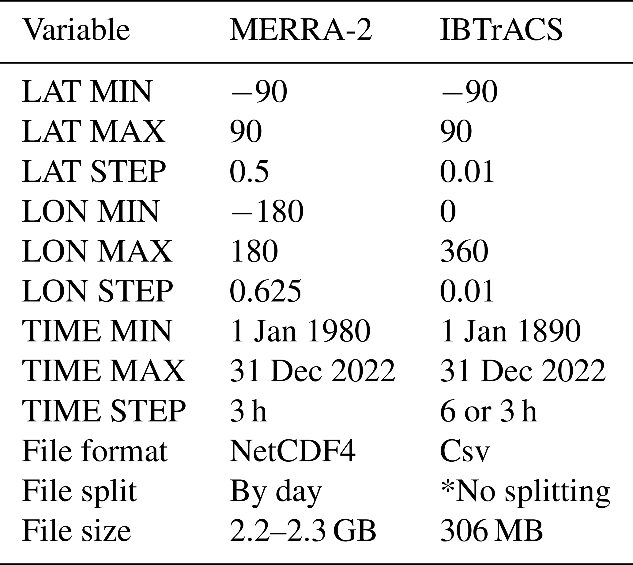
Although several reanalysis datasets are available, MERRA-2 was selected for this study primarily due to two reasons: (i) its spatial and temporal resolution is suitable for detecting TCG, (ii) its data format is convenient for ML model development, and (iii) TC-related information was assimilated into MERRA-2 via derived satellite products (Gelaro et al., 2017). Unlike some TC metrics such as intensity or accumulated energy that require detailed inner-core structure, TCG is a process that is largely governed by environmental conditions. With a resolution of 0.5° MERRA-2 is therefore expected to capture the overall environmental conditions for DL purposes. Note that the MERRA-2 dataset provides gridded atmospheric data that includes 11 key meteorological variables at standard pressure levels, spanning the global domain from 90° S to 90° N latitude (at 0.5° resolution) and from 180° W to 180° E longitude (at 0.625° resolution). The dataset is available from 1 January 1980, to 31 December 2022, with data sampled every 3 h. Each daily file contains 8 time slices and is stored in NETCDF4 format, with a file size of approximately 2.2–2.3 gigabytes.

One limitation of the MERRA-2 dataset as compared to other reanalysis datasets is that this dataset contains a single resolution of 0.5×0.625°, while other reanalysis datasets such as ERA5 provide higher resolution up to 0.25° at an hourly interval. Using such higher-resolution datasets is certainly an advantage, as it can help optimize ML models. However, we note that most current global climate projection outputs are given on 0.5 to 1° resolutions. Thus, using 0.5° data can help better demonstrate the usefulness and facilitate the applications or finetuning of our DL models for reconstructing TC climatology from global climate outputs as designed. While ERA5 is considered to be among the best for climate reanalysis and DL model development, whether ERA5 is better than MERRA-2 in terms of TC climatology at the 0.5° resolution has not been demonstrated. In this regard, our choice of MERRA-2 can be considered as a pre-learning step, which can be easily refined with ERA5 or any other climate datasets. For the purpose of implementing and evaluating TCG-Net, the MERRA-2 data is therefore sufficient.

Along with the use of MERRA-2 dataset for training, the International Best Track Archive for Climate Stewardship (IBTrACS) (Knapp et al., 2010) was also used to label all TCG events and locations, which contains global TC records. Specifically in the WNP basin, the Joint Typhoon Warning Center records in IBTrACS are selected, which contains data from 1 January 1890 through present day, sampled every 3 h and archived in a single CSV file. The fact that this IBTrACS dataset is structured with the same synoptic times as the MERRA-2 dataset is useful, because it allows us to pair these two datasets for supervised DL. Details of these datasets as well as their corresponding variables are summarized in Table 1.

Table 1 A list of variables and their corresponding ranges in the MERRA-2, and IBTrACS, raw datasets.

2.2 Data pre-processing

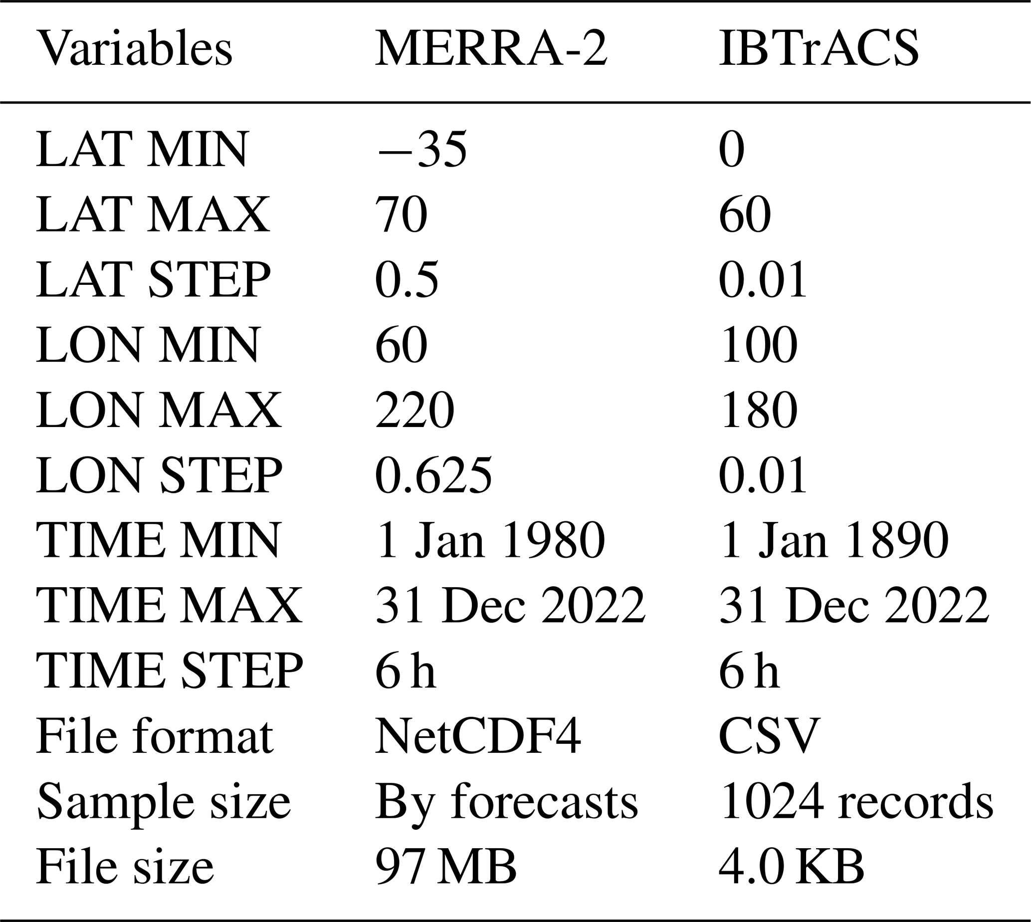
Given that MERRA-2 and IBTrACS datasets have their different format, structure, and parameters, it is necessary to first synchronize these datasets before any DL training can be carried out. For this data pre-process step, we convert the longitude axis of MERRA-2 from $[-\mathrm{180}:+\mathrm{180}]$ to [0:360] to match with the coordinate definitions in IBTrACS, which is needed so that the latitude and longitude values of IBTrACS can be located properly on the MERRA-2 coordinate grids for data extraction. In our study, a domain of a size [35° S–70° N] × [60–220°] in the Pacific Ocean is then extracted from the global MERRA-2 dataset. For each MERRA-2 file, a timestamp is output at an interval of 6 h to match with the best track data (note that the original MERRA-2 dataset consists of daily data files at an interval of 3 h). All details of these data outputs after pre-processing MERRA-2 and IBTrACS are provided in Table 2. The corresponding pre-process workflow is thoroughly described in our Zenodo repository (Le et al., 2025).

Table 2 Pre-processed data format and structures obtained from the MERRA-2 and IBTrACS datasets to train DL models.

2.3 Supervised dataset design

With the pre-processed data described above, the next step is to generate a labeled dataset for supervised ML models. Specifically for the study of TCG, we need a binary dataset that indicates whether or not a TCG event occurred in the WNP basin needed for the reconstruction of TCG climatology. The process of creating such a binary dataset is critical, as it must include not only positive TCG cases but also a well-designed set of negative samples. Such a requirement of both well-designed positive and negative samples is required for ML models to effectively learn the distinct features between TCG and non-TCG conditions. On one hand, a strong contrast between positive and negative samples increases the likelihood that ML models will identify key patterns, thereby improving performance. Nevertheless, the selection of positive and negative samples must also align with practical applications and purposes in climate research. In fact, the criteria for labeling positive/negative TCG events vary depending on the specific type of TCG climatology as will be shown in the Sect. 4. In this study, we follow NK2024 and define a positive TCG event as the first time a storm was recorded in the best track data. One could also define a TCG as the first moment that a tropical depression stage is recorded to make sure TCG characteristics are well-defined for DL training (Kieu and Nguyen, 2024). However, our choice of the first time that a TC was recorded in the best track herein has the benefit of training a DL model that can detect TCG earlier, and so we will use this definition to label a positive TCG event. Some additional steps to handle the uncertainties in this TCG timing will be further presented in our data enrichment in Sect. 3.3.

With the above definition of positive TCG labels, we can now scan through all TC track histories and take the first recorded location of each storm to create a data domain corresponding to positive TCG events. Given the typical scale of TCs, this positive TCG domain is chosen to be a square box of size 18×18° centered on the first recorded TCG location, which is equivalent to roughly 33×32 grid points with the MERRA-2, 0.5° resolution. Finally, all relevant information related to a TCG event including its longitudes, latitudes, date, and time was stored in a csv database to facilitate our data sharing and input to the DL interface.

For the negative-labeled TCG data, the issue turns out to be more subtle as discussed in Kieu and Nguyen (2024). Depending on the context and applications, one can in fact have several different ways to define a negative TCG event. From the practical perspective, we propose in this study two different sampling strategies for negative-TCG labels. The first strategy, referred to as the Past Domain (PD) strategy, uses temporal context to distinguish between positive and negative labels, i.e., predict when the TCG forms. Specifically, for each positive TCG event occurring at time t, all samples within a past window from t−k to t are labeled as positive, capturing the precursors leading up to the TCG time at t=0. All earlier samples from $t-k-\mathrm{1}$ up to time $t=-N$ further back in time are labeled as negative. This approach aims to answer the question of why a TC forms at a specific time but not earlier. A key advantage of this strategy is that it preserves the geographical location between positive and negative samples while introducing temporal separation. However, depending on the chosen value of k, there may be some overlap in favorable environmental conditions between the positive and negative samples.

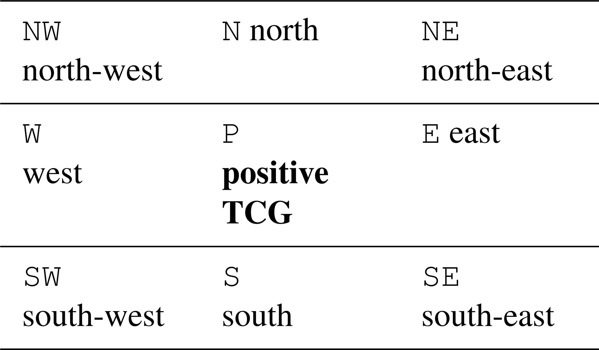
The second approach for generating negative TCG data is referred to as the Dynamic Domain (DD) strategy. In this approach, for each positive TCG event at time t, we consider the surrounding spatial regions as negative samples. Specifically, we define eight adjacent regions around a positive TCG location, including the north-west, north, north-east, east, south-east, south, south-west, and west directions, as negative-TCG labels (see Table 3). These eight surrounding domains can be also shifted back in time, similar to the PD strategy to further account for the uncertainties in the timing of TCG recorded in the best track. This type of domain selection for negative TCG data helps answer a question of why TCG occurs in one place but not in other places at the same day/time. One could randomly choose one of the eight negative domains to construct a more balanced binary dataset, as in NK2004, or choose all eight domains to increase the sample size. Unlike the PD approach, we note that this DD task will have a small chance of including a co-existing TC in the negative samples. This issue can be addressed by simply checking if there is any co-existing TC nearby within the negative TCG domain, and remove this domain or filter a TC out (Nguyen, 2023). In this study, we use a simple approach of discarding all negative TCG domains that have a co-existing TC to avoid complications with changing environmental conditions due to vortex removal processes. This affects < 1 % of all data points as we have in the WNP basin, as most TCG in this basin rarely overlap within a domain of an 18°×18° area.

Table 3 Illustration of a TCG data labeling strategy based on the dynamical domain approach, for which a positive TCG label at one location is surrounded by 8 negative TCG labels for the sampling strategy. The bold text highlights the location with a positive TCG label, where the TCG appears.

As part of constructing the binary TCG dataset described above, it is important to note that TCs can form at any time of day, whereas the IBTrACS, dataset provides records at fixed 6 h intervals. Consequently, the actual genesis location of a TC may differ slightly from the position recorded in the best-track data. This spatial discrepancy typically depends on storm motion and the algorithms used for detecting vortex centers at operational centers. In this study, we assume that the TCG location does not vary significantly within a 6 h window, which provides a reasonable basis for maintaining consistency in our binary TCG dataset design. This assumption also allows us to use the first recorded time in the IBTrACS, dataset to define positively labeled TCG samples, which by convention are assigned a label of 1. All negative samples are labeled as 0.

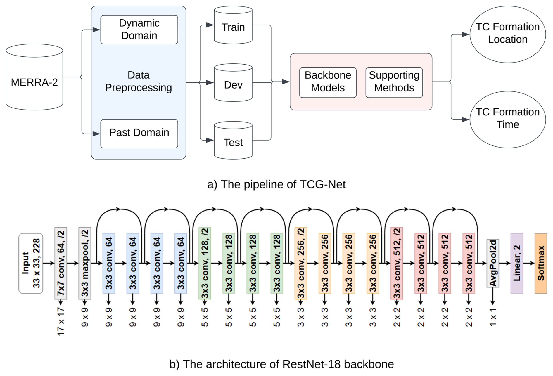
Figure 1 (a) The pipeline of TCG-Net for reconstructing TCG climatology from the MERRA-2 dataset, and (b) the core DL model based on the ResNet-18 architecture used for TCG reconstruction in this study.

3 TCG-Net: Deep Learning Framework

3.1 Model design

Recent advances in DL research have demonstrated substantial potential across a range of fields, including image recognition, natural language processing, autonomous driving, and weather prediction (Gao et al., 2018b; Kim et al., 2019a; Giffard-Roisin et al., 2020; Miller et al., 2017; Su et al., 2020; Bi et al., 2023; Weyn et al., 2021). In the context of TCG applications, several DL approaches using satellite imagery data and TCG predictors have been proposed (Zhang et al., 2015; Park et al., 2016; Matsuoka et al., 2018; Zhang et al., 2019; Kim et al., 2019a). To make further use of climate data for a broader context, NK2024 employed a convolutional neural network (CNN)-based DL framework and showed promising results for TCG application despite limited training data. Their study underscores DL's image recognition capabilities, which enable the detection and analysis of relevant environmental patterns from climate meteorological fields for TCG prediction.

Given such promising performance of the CNN-based models as well as the features tailored specifically for TCG reported in NK2024, we propose TCG-Net, a deep learning architecture designed to predict tropical cyclogenesis by leveraging atmospheric reanalysis data from MERRA-2. The pipeline begins with data preprocessing, where inputs are divided into dynamic and past domains to capture both current atmospheric conditions and historical context. These data are then split into training, development, and testing sets to support reliable model evaluation. At its core, TCG-Net uses backbone models, e.g., CNN or RestNet, to extract meaningful features. Supporting methods, including attention or temporal fusion techniques, enhance the model’s ability to capture complex patterns associated with cyclone formation. The framework jointly predicts two key outputs namely: the location and timing of cyclone genesis. The entire workflow is shown in Fig. 1a.

In this study, we use ResNet-18 as the primary backbone model. It consists of eight residual blocks, preceded by an initial convolutional layer for input embedding, and followed by a fully connected layer with a softmax activation to predict the probability of storm occurrence, forming a total of 18 layers (Fig. 1b). This architecture differs slightly from that used in NK2024, as our study employs the MERRA-2 dataset, which lacks several environmental variables such as CAPE and tropopause-level features. Consequently, the ResNet-18 model required refinement and testing to achieve optimal performance, which differs somewhat from the architecture tailored for the NCEP Final reanalysis dataset in NK2024.

It is noted that our experiments with alternative DL architectures such as more convolutional layers, vision transformers, or pre-trained models all displayed minimal improvement over the performance of the adapted ResNet-18 used in this study. While this conclusion is obtained from the few models that we have tried, it is possible that the TCG problem has limited predictability or MERRA-2 dataset may contain limited information for TCG at 0.5° resolution that more sophisticated models or architectures could not help learn further. This is a known problem in DL training, which explains why a simple CNN model could reach as good a performance as other models (Brigato and Iocchi, 2020). Note also that complex models with more parameters generally have a very high “capacity” to learn. When the training data does not contain a variety of patterns, a high-capacity model can easily memorize the training data, including its noise and idiosyncrasies, instead of learning generalizable features. This leads to good performance on the training set but poor performance on unseen data, which is known as overfitting. Thus, the ResNet-18 model was adapted herein for our TCG reconstruction problem.

3.2 Evaluation metrics

To monitor and verify our DL models, we employ several metrics from traditional classification problems for training models and meteorological metrics specific for TCG climatology such as seasonal or spatial distributions for validation. For the DL training, the performance of our DL model loss fucntion is based on Precision (P), Recall (R), and F₁ scores. These scores are useful due to the inherent class imbalance for which TC occurrences (positive samples) are significantly fewer than non-TC cases (negative samples). By definition, P measures the proportion of correctly identified TC instances out of all instances predicted as TC:

$$\begin{array}{}\text{(1)}& \text{Precision}={\displaystyle \frac{\text{TP}}{\text{TP}+\text{FP}}},\end{array}$$

where TP (True Positives) represents correctly detected TCs, and FP (False Positives) denotes non-TC cases incorrectly classified as TC. A high precision ensures that the model minimizes false alarms, which is critical for reliable early warning systems.

In contrast, R quantifies the proportion of actual TC occurrences that the model successfully identifies:

$$\begin{array}{}\text{(2)}& \text{Recall}={\displaystyle \frac{\text{TP}}{\text{TP}+\text{FN}}},\end{array}$$

where FN (False Negatives) represents actual TCs that the model fails to detect. A high recall ensures that most TC events are captured, reducing the risk of missing critical storm formations.

To balance take into account both P and R, we use the F₁ score defined as:

$$\begin{array}{}\text{(3)}& F_{\mathrm{1}}\text{-score}=\mathrm{2}\times {\displaystyle \frac{\text{Precision}\times \text{Recall}}{\text{Precision}+\text{Recall}}}.\end{array}$$

A high F₁ score indicates a good trade-off between false alarms and missed detections, making it a crucial metric for assessing the reliability of TC detection models. Since missed TCs can lead to severe consequences, while excessive false alarms may reduce trust in predictions, optimizing both P and R is essential in operational forecasting.

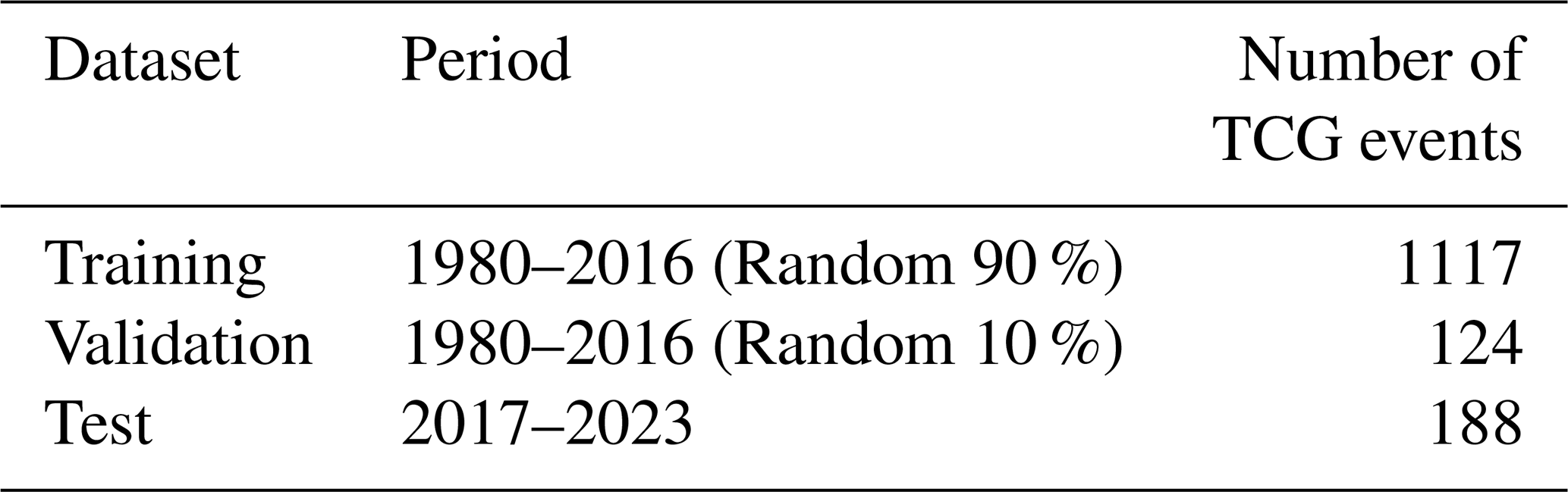
With the above metrics, we could train a DL model to maximize the model F₁ score performance for any period, which is set by default to be 10 % of data from 1980–2016 for validation in this study (see Table 4). Note that these category verification metrics are needed to train the ResNet-18 model. Whether the model can perform well for our TCG reconstruction depends further on its performance over other climate evaluations such as seasonal distribution or spatial distribution as presented in the Result section.

Table 4 The statistic of training, validation, and test sets.

3.3 TCG data imbalance

Given the uncertainty in the TCG timing in the best-track and the severe class imbalance of TCG data caused by the limited number of TCG events, it is essential to apply some additional techniques to mitigate this imbalance before training a DL model. One approach, as described in Sect. 2.3, involves temporal data enrichment using past windows, which is mostly suitable for the PD labeling strategy. This same past data window enrichment can also be extended to the DD labeling strategy by using the data from previous cycles to help increase the number of positive labels. While this data encrichment could help address the uncertainty in the TCG timing, the imbalance ratio for the DD labeling strategy is always 1:8. Thus, adding more past data would not help reduce the imbalance ratio.

To address this class imbalance issue, we also introduce a complementary method, known as the Random UnderSampling (RUS) approach. Specifically, the RUS method controls the ratio between negative and positive TCG samples in the training dataset. For example, a RUS value of 1:4 maintains four negative samples for every positive one. Since this undersampling strategy may still leave a slight imbalance, we further apply class weighting in the loss function to emphasize the minority class during training. This technique increases the loss penalty for misclassifying rare (positive) cases, encouraging the model to better capture them. Two types of class weights are used in this study, which include (i) the balanced class weight (default) and (ii) the proportional class weight defined as $\mathrm{1}/\mathrm{5}$ RUS. Together with the temporal data enrichment, the RUS-based sampling and class weighting strategies can improve the performance of our DL models for TCG reconstruction, surpassing the simple hyperparameter optimization based on the F₁-score criterion.

3.4 TCG detection

With the output from the ResNet-18 model, we can finally produce a TC probability map for climate reconstruction. Given two different strategies for data labeling based on the DD and PD methods, detecting a TCG event and assigning it to a point in space and time require some specific details.

For the PD strategy, it focuses on the temporal aspect of TCG prediction, which generates negative samples at the same location as positive samples. Thus, TCG detection for this approach is straightforward, as one can simply choose any fixed location at time t, obtain data at that same location from previous times t−i to time t, where i represents previous time steps, and then generate TCG probability for that fixed domain. With this strategy, one can obtain TCG probability for any area of interest, so long as the domain contains sufficient TCG labels during an interval $[-k,\mathrm{0}]$ where TCG even exits for model training. In this regard, PD can provide TCG information for any location as expected.

With the DD strategy, we recall that one wants to extract the map information of TCG over the entire WNP basin at any given time t such that the spatial variation of TCG can be examined. So, our approach for reconstructing TCG for this DD strategy is to divide the WNP basin into a grid of 5° ×5°, and apply the ResNet-18 model to a domain located at the center of each grid point separately. This way, we can detect TCG for the entire grid simultaneously at time t. Assuming that a positive TCG event is found when TCG probability is larger than a certain threshold (e.g., 0.5), one can reconstruct a map of TCG locations at any given time t as expected. Because of these different purposes in extracting TCG information for the PD and DD strategies, our evaluation and interpretation of the model performance for TCG climatology have to be therefore based on separate metrics and criteria, as will be presented in the next section.

4 Results and Discussion

4.1 TCG-Net benchmarking

To first have a general picture of how the ResNet-18 model is optimized for our TCG prediction problem, Fig. 2 shows the precision, recall, and F₁ score obtained from the test set for the PD and DD tasks. Note that for the PD strategy, we focus on a fixed domain over a part of the WNP basin whose TC activity has the most influence on Vietnam's coastal region ([0–30° N]–[100–150° W]). This domain choice is of course application-specific and so it should be adjusted for each region of interest. Given this arbitrary choice of area for the PD strategy, this section will report all results over the aforementioned domain.

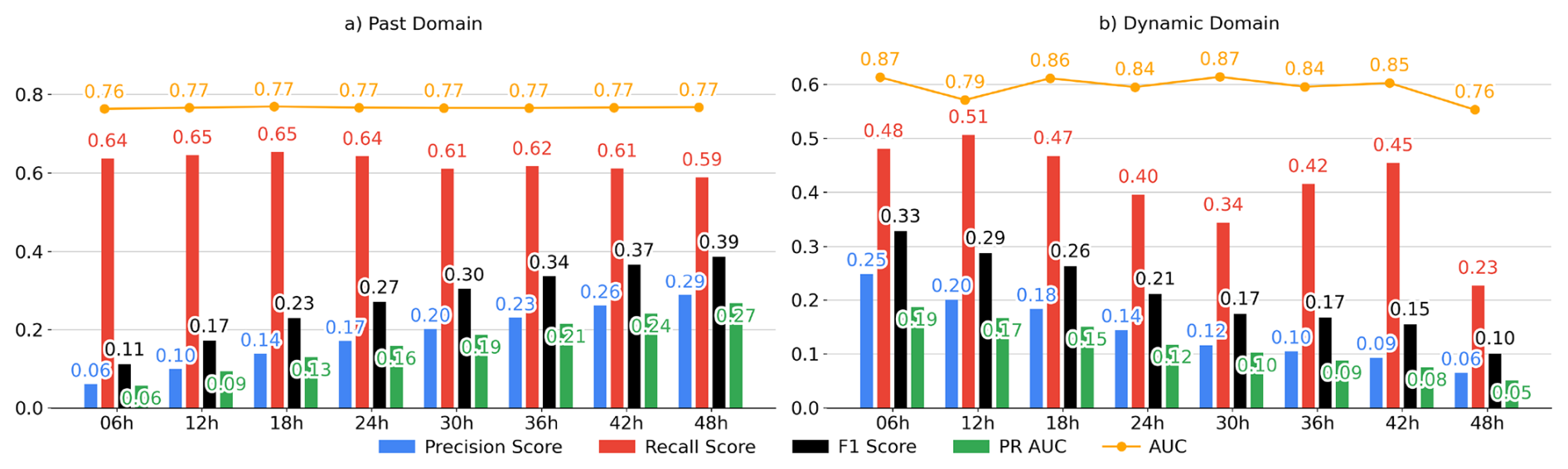
Figure 2 Overall performance of TCG-Net in terms of Precision (blue), Recall (red), F₁ score (black), precision–recall area under the curve (PR-AUC, green) and area-under-the curve ROC (AUC-ROC, yellow) for the TCG prediction on (a) Past Domain, and (b) Dynamic Domain.

As can be seen in Fig. 2, the temporal feature enrichment plays a significant role in the performance of the ResNet-18 model. For the PD task, a longer period of feature enrichment generally gives a better precision score without much reduction in the recall performance (0.57–0.62), thus allowing for a higher F₁ score for longer enrichment windows. This is consistent with the precision–recall area under the curve (PR-AUC) score (see green columns), which shows better forecast skill for longer data enrichment windows, even for highly-imbalanced data. In fact, the area-under-curve ROC (AUC-ROC) score is of 0.76–0.77 for all enrichment windows, indicating that the model could capture TCG occurrence beyond a random chance as expected.

Physically, such behavior of the PD sampling strategy means that including more past information at a fixed location generally helps improve the accuracy of the model performance in capturing TCG in that area. This is because past information around the TCG moment recorded in the best track contain sufficient signals of TCG that help ResNet-18 learn better. Note however that the overall P and R scores are still relatively low even when including all past information up to 48 h. Thus, the overall F₁ score for detecting TCG from MERRA-2 dataset is much less as compared to that directly from satellite image data (see, e.g., Chen et al., 2020; Wimmers et al., 2019)

As discussed in Nguyen and Kieu (2024), the low performance of DL models in detecting TCG from climate reanalysis datasets could also reflect the fact that the TCG problem has limited predictability that including more information would not help improve its performance, consistent with the high false alarm rate in physical-based models. This can be seen also in our attempt to apply other methods such as random forecast, XGBoost, or climatological method based on the genesis potential index in Fig. 3. All of these attempts indicate a similar low skill in capturing TCG, which shows an F₁-score in the range of 0.3–0.32 even with the best TCG-Net model's performance.

Another potential reason for such a low F₁ score is the MERRA-2 data itself, which may not cover all possible environmental patterns for rare extreme events like TCG. This highlights the difficulty in reconstructing TCG climatology from climate reanalysis data as compared to that from satellite images.

For the DD strategy, the dependence of the model performance on the temporal enrichment is opposite. Specifically, the F₁-score is optimal for very short enrichment during a 6 to 12 h window, and it quickly decreases when the time window is longer (see Figs. 2b and 4). Practically, this means using past information as data enrichment to explain why a TC forms at one place but not at other places will not help if one includes more past information.

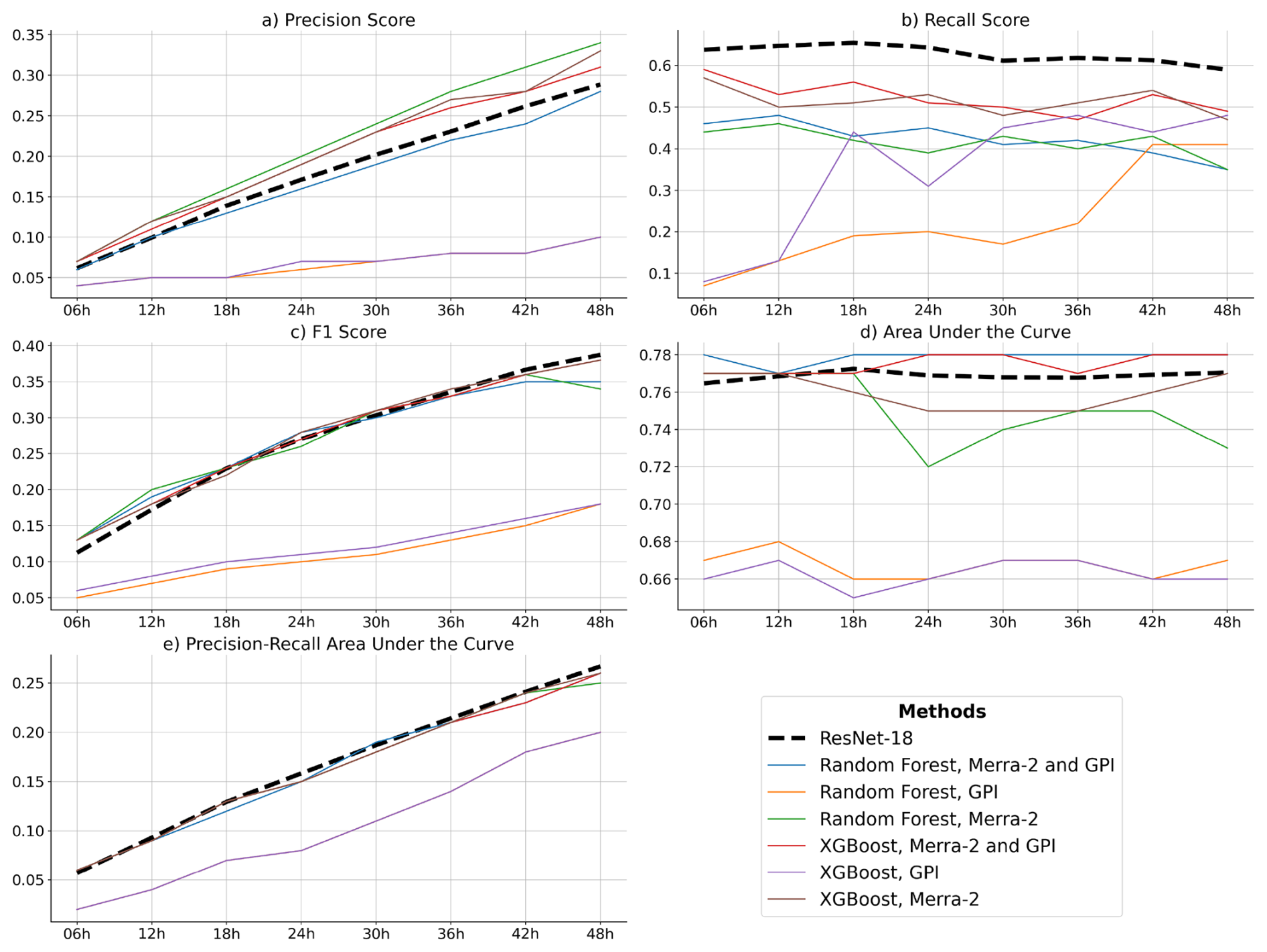
Figure 3 Comparison of the model performance for the Past Domain task between TCG-Net and traditional classification models, i.e., XGboost and random forest, which are enhanced by including the climatological Genesis Potential Index (GPI). The thick dashed line denotes the performance of TCG-Net with ResNet-18 backbone.

This result is also expected if one recalls that the main aim of the DD strategy is to search for where a TCG occurs at any given time. So, the model is trained to detect spatial TCG signals rather than from temporal information. Enriching the DD strategy by including more past information introduces more irrelevant environmental information from the past (i.e., negative labels) that causes more bias towards negative samples. This explains why the R score (blue columns in Fig. 2b) decreases quickly with a longer enrichment window. As a result, the DD strategy exhibits a declining in both F₁ and PR-AUC score, indicating that the model's overall reliability in detecting TCG decreases when too much past information is used, even when the model is still able to distinguish TCG from random variation (see the AUC-ROC curve in Fig. 2b).

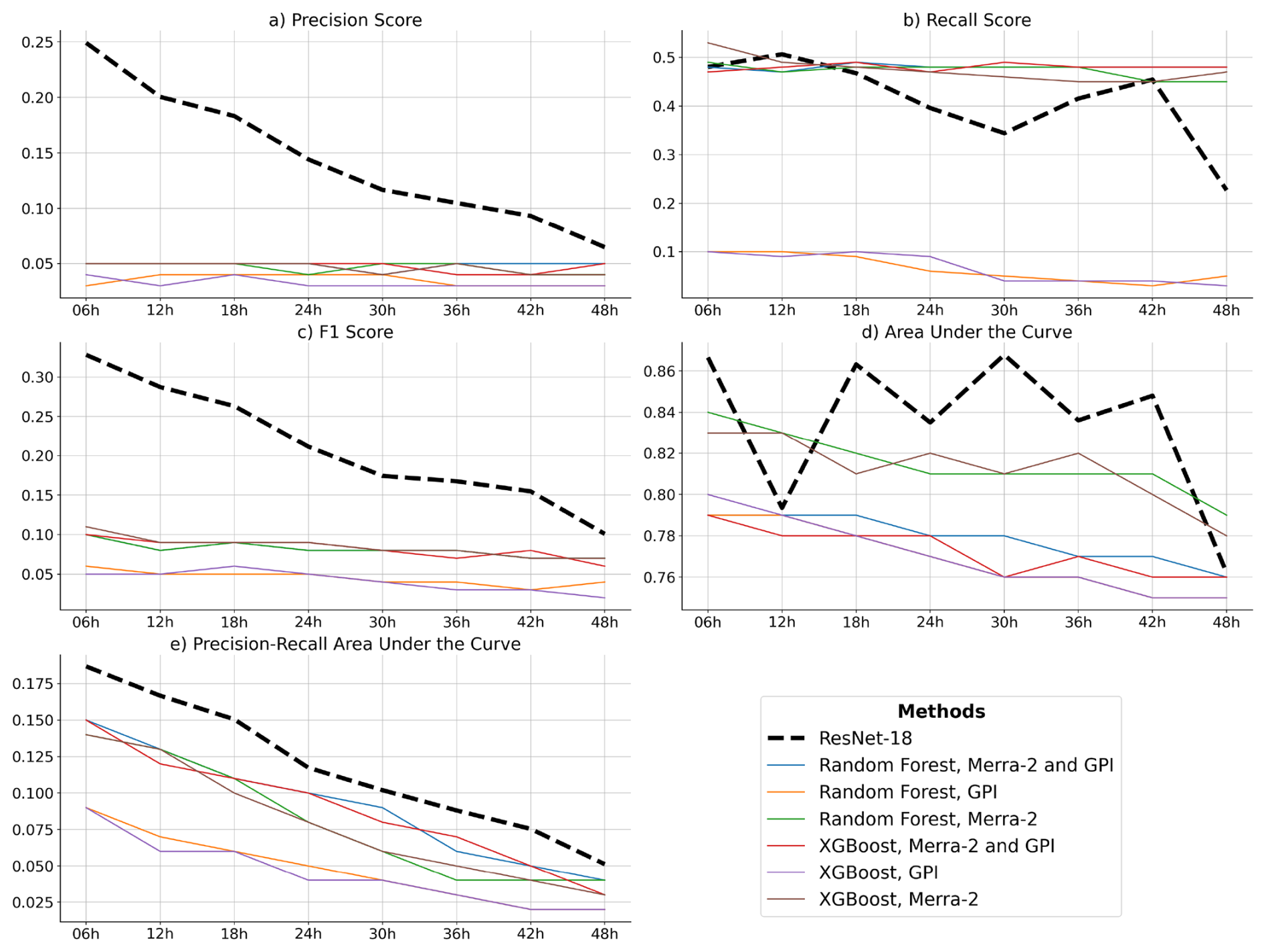
Figure 4 Comparison of the model performance for the Dynamic Domain task between TCG-Net and traditional classification models, i.e., XGboost and random forest, which are enhanced by including the climatological Genesis Potential Index (GPI). The thick dashed line denotes the performance of TCG-Net with ResNet-18 backbone.

4.2 TCG reconstructed climatology

With the optimized ResNet-18 model as presented above, our next attempt is to examine the seasonal distribution of TCG frequency. Here, the seasonal distribution is defined as the averaged ratio of the count of TCG events over the entire WNP basin detected in a given month to the total number of TCG events detected each year, which can be interpreted as monthly TCG frequency. To avoid the issue with an arbitrary choice of the domain location for the PD strategy, we will generate the monthly TCG frequency only for the DD strategy in this analysis.

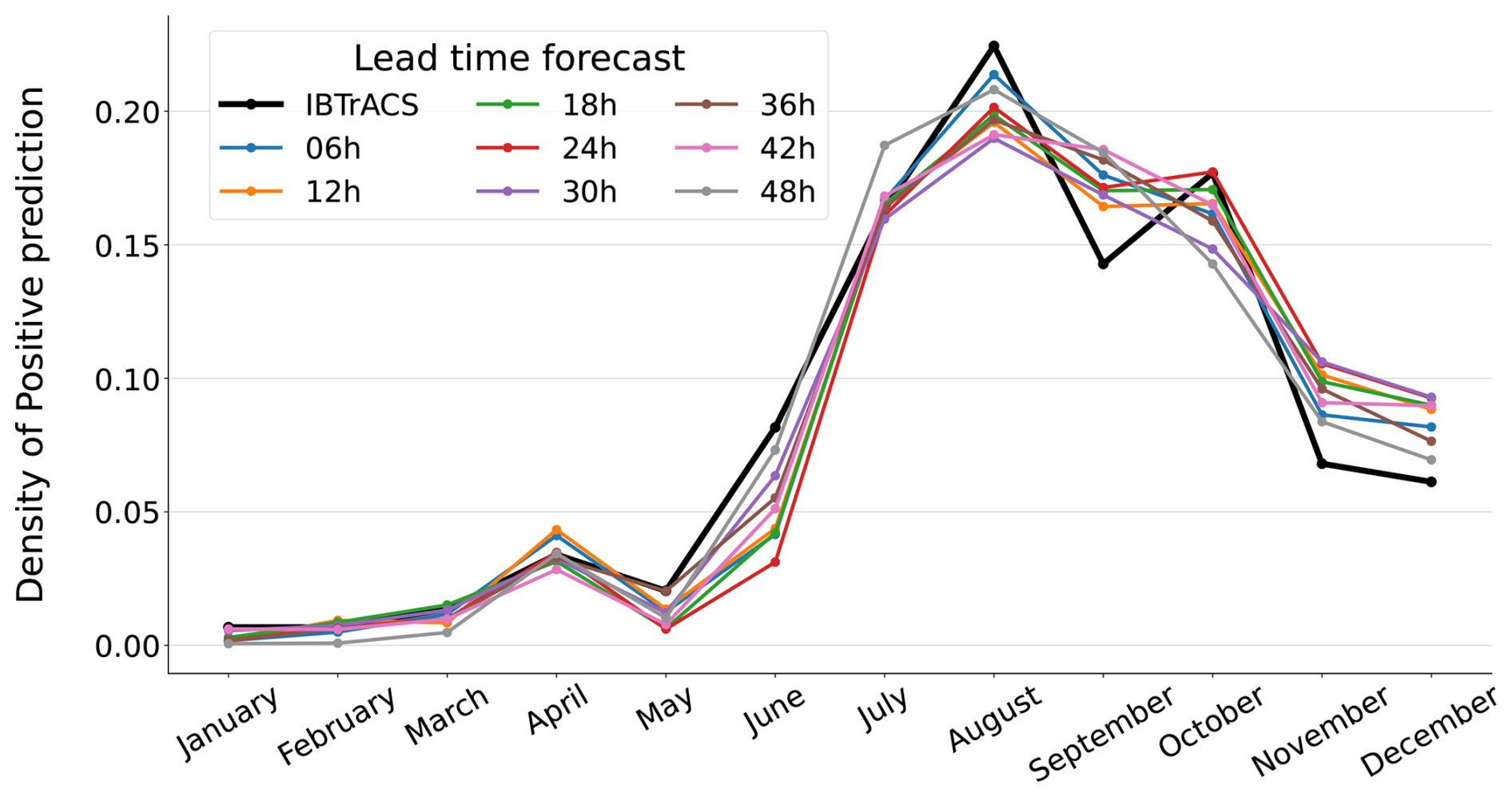
Figure 5 Monthly distribution of TCG frequency detected in the WNP basin from the test data (2017–2022), using the best-tuned ResNet-18 model for the DD strategy with data enrichment windows from 6 to 48 h. The black solid curve denotes the TCG frequency obtained from the best track during the same time period.

As seen in Fig. 5, the ResNet-18 model could reproduce well the overall seasonal distribution of TCG during a test period from 2017–2022, with a peak of TC activities in July–October, followed by an inactive period in January–April, similar to the observed TCG frequency. In addition, the ResNet-18 model appears to also reproduce the double peaks of TCG frequency in August and October consistent with the observed distribution, albeit the dip of TCG frequency in September is not as clear as that from the best track. During the peak period, note that the trainings with longer enrichment windows (i.e., 36–48 h) tend to generate more positive TCG events than those with shorter windows (6–24 h), suggesting that early signals of TC formation become more detectable as more past information is included.

Towards the end of the peak season (during November–December), note that TCG-Net tends to produce more TCG than the observation, while it underestimates the TCG frequency during May–June. These differences indicate a common fact in TC climate research that optimizing a DL model based on one specific metric such as F₁ score, precision, or recall, would lead to biases in other metrics (e.g., Vu et al., 2025). Another possible reason for this discrepancy could also be due to the limited ability of large-scale environments in reproducing the seasonal variability of TCG (e.g., Tippett et al., 2011; Menkes et al., 2012). Regardless of such differences due to different tuning metrics, the consistency of the seasonal TCG reconstruction by the ResNet-18 model across the enrichment windows suggests that ResNet-18 can understand the seasonal changes in large-scale environments for TCG as expected.

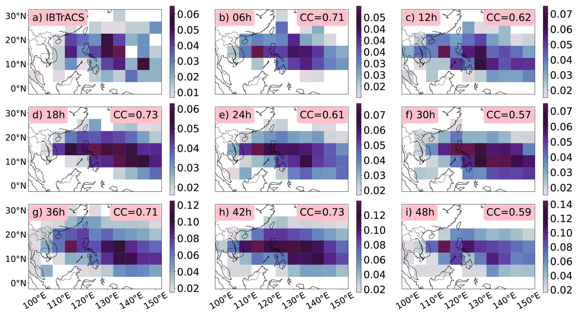
Figure 6 (a) The spatial distribution of the observed TCG density (shaded) during the 2017–2022 period as obtained from the best track; (b–i) 5-year average of TCG probability prediction that is obtained from the ResNet-18 model with different data enrichment windows from 6–48 h during the same test period as in (a). Note that different shading scales are used for different data enrichment windows so that one can better see the contrast between the areas of maximum probability for TCG predicted by the ResNet-18 model.

Along with the seasonal TCG frequency, another important climate metric to validate the ResNet-18 model is the spatial distribution of TCG climatology. In this regard, Fig. 6 shows the horizontal map of the TCG probability detected over the entire WNP basin, using the DD strategy with different enrichment windows from 6 to 48 h. Here, the shading in each 5° ×5° box represents the averaged probability of positive TCG predictions from the ResNet-18 model over the test period (2017–2022). For the observed TCG, the shading denotes however the actual number of TCG events occurs in each box, divided by the total number of TCGs during the 2017–2022 period (commonly known as TCG density in literature). Because the predicted and observed TCG density are proportional to each other, they can serve as a metrics to evaluate our DL model's performance from a different angle.

Overall, ResNet-18 could again reproduce well the TCG density distribution in the WNP basin during the 2017–2022 period, with clear TCG hotspots in both the East Philippine Sea and the South China Sea (SCS), with the spatial correlation in the range of 0.75–0.83. For long enrichment windows between 18–42 h, note that the ResNet-18 model tends to extend the TCG region too far east of the East Philippine Sea as compared to the observation. Despite the deterioration of ResNet-18's performance for longer enrichment windows, the overall spatial distribution of TCG probability is still distinct and concentrated in the central SCS, the eastern Philippine Sea, and the Vietnam coastal region. For the shorter data enrichment window of 6–12 h, the model could also provide a reasonable fit as compared to the observed distribution (Fig. 6b), although it is not as good as the longer windows or the seasonal distribution in Fig. 5. The correlation between the DL-detected and best-track TCG density peaks around 24–36 h windows, reaching the highest correlation of 0.83 for these windows.

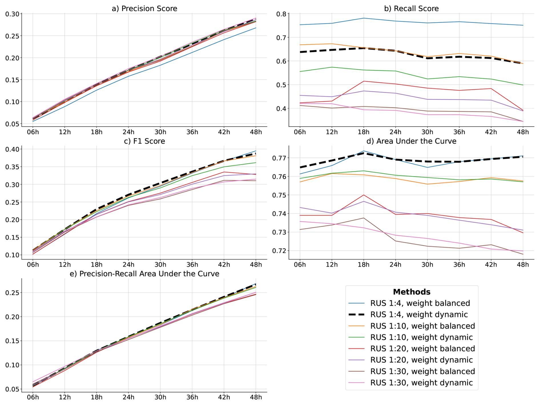
Figure 7 (a) The precision score P for the TCG prediction of TCG-Net using a range of the RUS ratio and class weight (solid colors) for the Past Domain task and the same sampling ratio for both the training and test sets; (b)–(e) similar to (a) but for the R, F₁, AUC and Precision-AUC scores, respectively. The dashed black line denotes the reference obtained from our best-tuned model. Note that weight balanced assigns fixed importance to each class based on frequency whilst weight dynamics adaptively adjusts sample or class importance.

It is worth noting that while the predicted TCG probabilities consistently peak in the eastern Philippine Sea, some localized maxima in the central SCS and along the Vietnamese coastline lack consistency across data enrichment windows. This variability reflects the inherent challenge of detecting early TCG signals in the SCS, which are typically weak and highly variable. As a result, ResNet-18 struggles to capture these localized signals effectively when optimized based on the F₁ score over the broader WNP basin. Unfortunately, the amount of available TCG data in the SCS region alone is insufficient for meaningful DL model training, making it difficult to resolve such inconsistencies given the current limitations of climate datasets. In addition, the test period from 2017–2022 may possess some unique characteristics that the model trained during the 1980–2016 period could not capture. Because of this, we could only reconstruct the TCG climatology using the DD strategy in this subsection, even though the PD strategy is more directly applicable for real-time forecasting purposes.

Aside from these local issues, the ability of our DL model in capturing the broad spatiotemporal patterns of TCG suggests that atmospheric signals associated with TCG become increasingly detectable when more relevant information is incorporated. From a practical standpoint, these results are significant because not only do they validate the performance of our DL model, but they also demonstrate that TCG can be predicted from large-scale environmental information, even at a spatial resolution of 0.5°. This result has two important consequences: (1) as long as climate models can reliably simulate the large-scale environment, it is possible to learn TCG patterns with DL models and derive TCG climatology without resorting to the more computationally expensive high-resolution dynamical downscaling, and (2) changes in TCG climatology can be captured through changes in large-scale environments, which are generally much more robust and reliable in climate projections than individual storm-scale features.

4.3 Sensitivity analyses

Given that the TCG dataset is highly imbalanced due to the rarity of positive TCG labels, it is important to examine how ResNet-18 could be optimized under various training data scenarios. For this purpose, Fig. 7 shows ResNet-18's performance with different RUS ratios as described in Sect. 3.3. For the sake of clarity, we show here the absolute RUS ratios with a fixed number of positive TCG labels (minority) while changing the number of negative labels (majority) according to each ratio displayed in Fig. 7. For each RUS ratio, a class weight value that adjusts the loss function is also provided, which controls the importance towards the positive TCG labels during training.

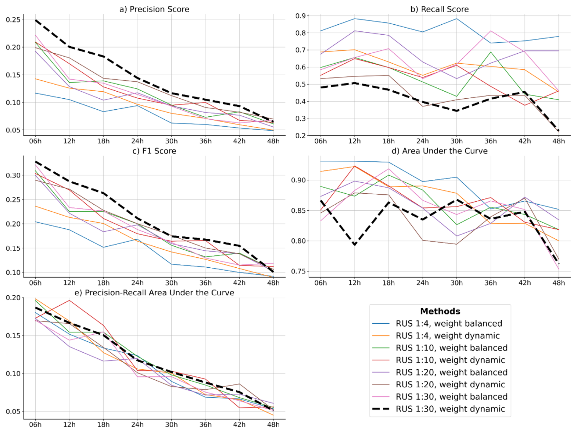
Figure 8 (a) The precision score P for the TCG prediction of TCG-Net using a range of the RUS ratio and class weight (solid colors) for the Dynamic Domain task and the same sampling ratio for both the training and test sets; (b)–(e) similar to (a) but for the R, F₁, AUC and Precision-AUC scores, respectively. The dashed black line denotes the reference obtained from our best-tuned model. Note that weight balanced assigns fixed importance to each class based on frequency whilst weight dynamics adaptively adjusts sample or class importance.

Figures 7–8 display a range of the R, P, and F₁ scores for different RUS ratios and class weights, using both the PD and DD sampling strategies. In general, a larger RUS ratio (i.e., more balance between positive and negative labels) tends to give higher P and R scores, thus resulting in a higher F₁ score for the PD strategy. The optimal RUS ratio of 1:4 (one positive label corresponds to 4 negative labels) combined with a class weight of 0.5 provides the best performance for the PD strategy in terms of detecting TCG, which is chosen as a default value in Fig. 2.

For the DD strategy, the model behavior is somewhat different because of the constrain that one positive TCG location is surrounded by 8 negative labels by design. Therefore, the data imbalance at any given time is always fixed for the training. When applying the data enrichment longer windows, the number of negative TCG labels increases rapidly because most of the days in the test period have no TCG. As a result, the imbalance becomes very small. For a reference, we show here only three RUS ratios of 1:10, 1:20, and 1:30 so one can compare their performance for the DD labeling strategy.

As seen in Fig. 8, the DD strategy performs best when the RUS ratio is 1:30, with a weight class of 0.2. Too small or too large RUS ratios both degrade the model performance. Consistent with the control performance shown in Fig. 2, all RUS ratio and class weight experiments also show best performance when the data enrichment window is around 0–12 h in terms of these scores, beyond which the performance of the DD strategy starts decaying rapidly. Such behavior is likely because the inclusion of larger negative samples from surrounding environment at farther back in time cannot help the model distinguish the positive labels, leading to a much lower R score. In contrast, too large RUS ratio means less over positive TCG data for training. Thus, the overall F₁ score is higher for a RUS ratio of 1:30 and a shorter time window as seen in Fig. 8.

In addition to the model optimizations based on the RUS ratio, feature enrichment time windows, and class weights as presented above, there are many other factors related to model architecture or hyperparameter settings that must also be considered to achieve optimal performance. Many of these aspects are excessively granular and so we cannot discuss every single one of them here. However, it is of interest to note that no single DL model is universally optimal across all weather features and spatial-temporal scales, particularly given the current limitations of available climate datasets and DL architectures.

Along with the above hyperparameter sensitivity, we also experimented with a range of model architectures, from a relatively simple CNN to more complex DL frameworks. However, their performance was broadly comparable in terms of F₁ score, precision, and recall (results not shown). Therefore, in this subsection, we keep the ResNet-18 architecture fixed and focus on sensitivity experiments involving different hyperparameter configurations or sampling strategies, rather than presenting results for different DL architectures.

4.4 Feature Importance Analysis

One last critical question in developing a DL model when the training data does not contain sufficient information is how to make full use of the data to optimize the model's performance. This process, known as feature engineering, becomes more significant when one tries to understand why we get what we see from DL model's output. Instead of running a DL model as a black box with all possible input data channels, exploring the importance of different input data can help better understand the role of different physical information in the model prediction that we wish to examine from a physical standpoint.

This subsection provides several additional analyses that employ a different set of input channels to see how effectively ResNet-18 could perform with limited information. Specifically, we examine two analyses that (1) use a set of features known to be of importance for TCG from previous studies, and (2) apply an automatic feature filter based on the rank of input channels. While this is often considered to be a part of model tuning, we treat them separately in this subsection as choosing the right input channels will have significant implications in our further understanding of TCG processes.

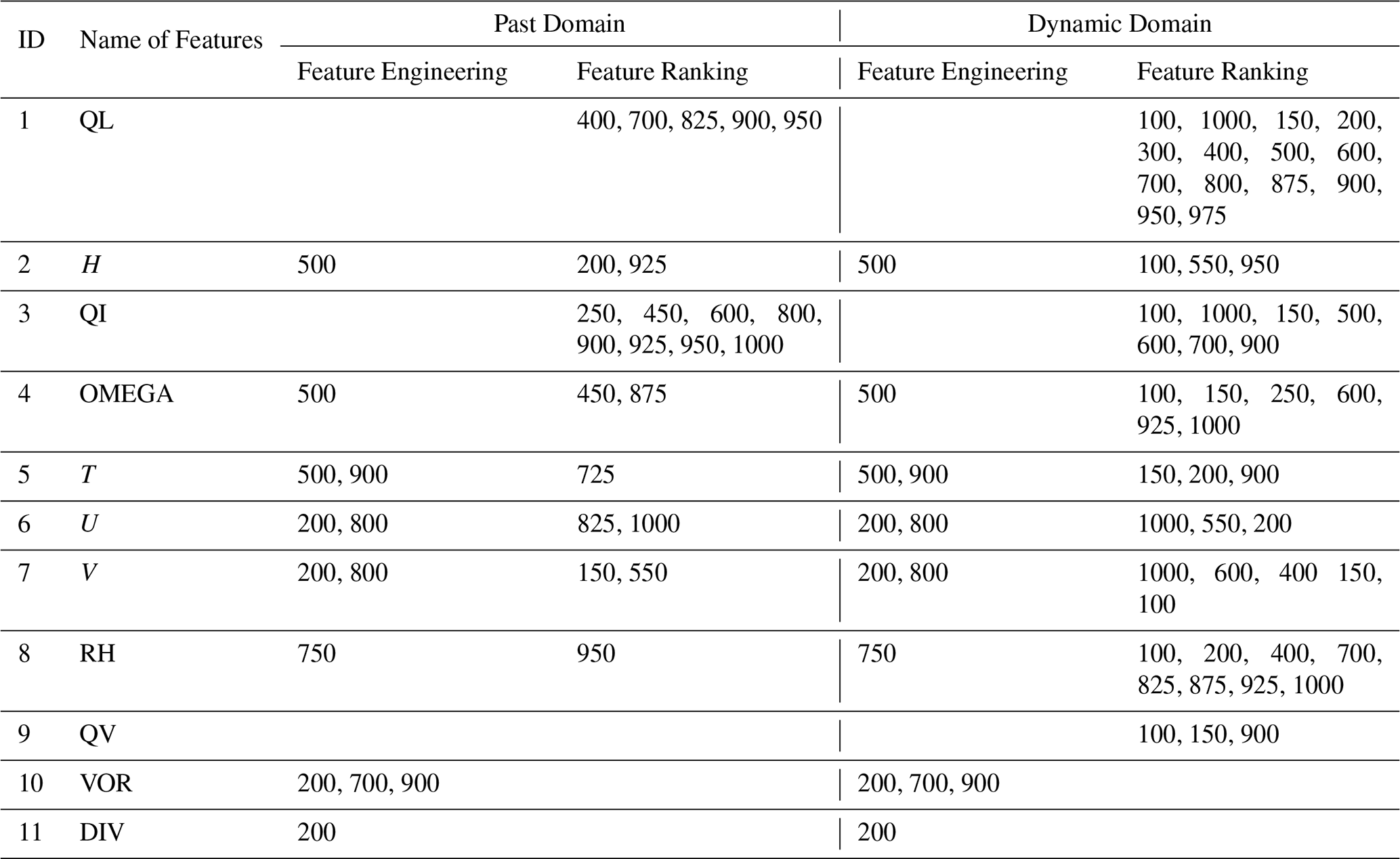
Table 5 List of features selected using the feature engineering and feature ranking filter approach as obtained for each labeling strategy during the training period.

For the first approach (hereafter referred to as feature engineering), input channels are based on their well-documented importance from previous observational and modeling studies (see, e.g., Gray, 1968; Riehl and Malkus, 1958; Yanai, 1964; Zhang and Bao, 1996; Bister and Emanuel, 1997; Ritchie and Holland, 1997; Simpson et al., 1997; Molinari et al., 2000; Nolan et al., 2007; Nguyen and Kieu, 2024; Kieu et al., 2023). These specific channels are useful for DL model development, because not all meteorological data contains independent information about TCG. Thus, using a subset of atmospheric variables that capture the strongest TCG signals will help DL models to learn better TCG processes. Following Nguyen and Kieu (2024), this feature engineering selects a group of variables on several low, middle, and high pressure levels as shown in Table 5.

For the feature filtering based on their importance ranking (hereafter feature ranking), data channels are automatically selected by their contribution to the prediction score instead of depending on specialized knowledge as for the feature engineering approach. This can be done by ranking all input features in terms of their mean activation values of the first filter from our best-tuned ResNet-18 model. Selection is then proceeded iteratively as follows. First, the channel with the highest score in the scoreboard is chosen and removed from the pool. Next, we eliminate any remaining layers that are highly correlated with the chosen channel, based on the Pearson R correlation threshold. Finally, the progress is continued until all remaining features are either selected from their score or discarded, depending on the threshold that is used to stop the selection.

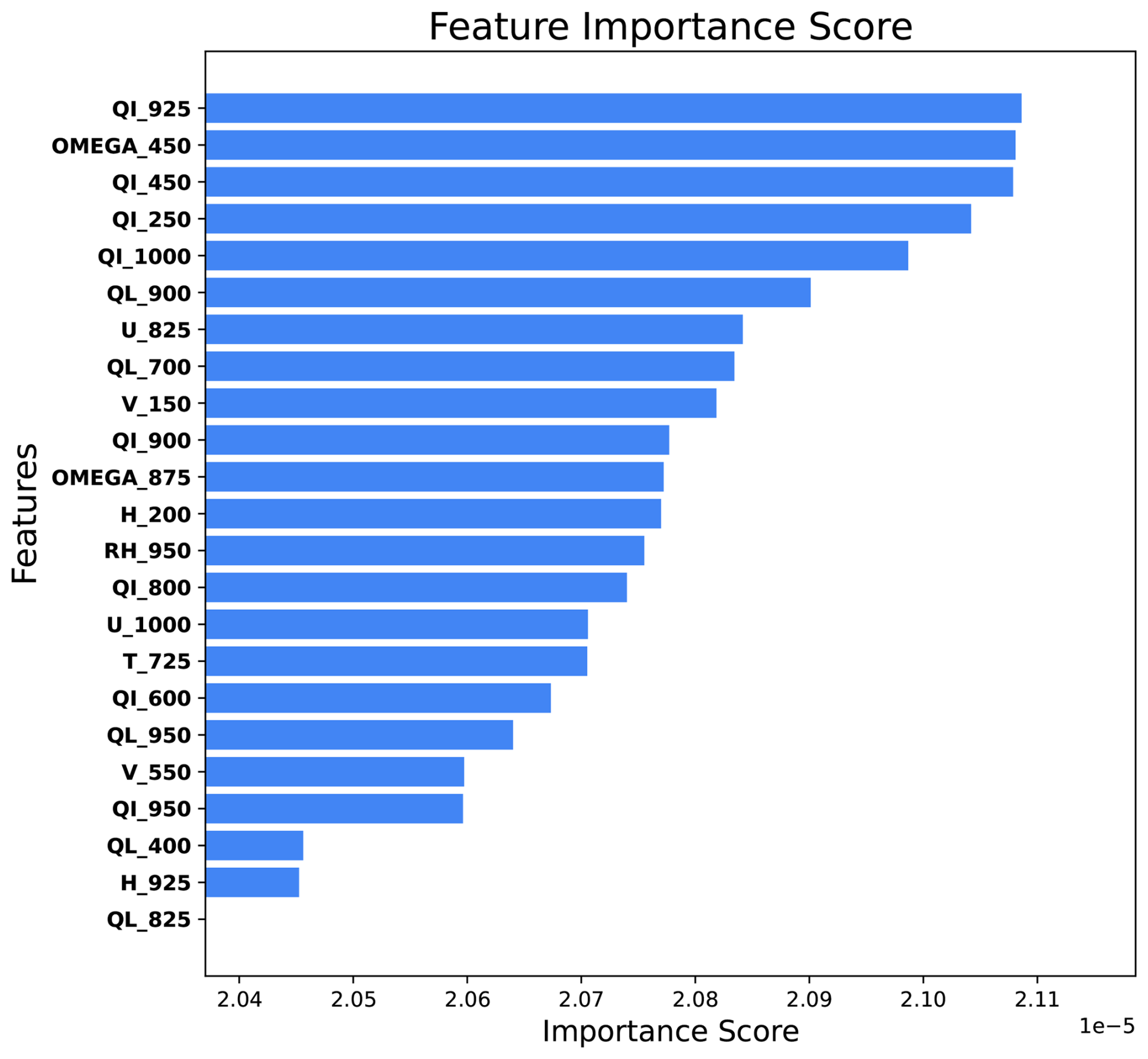
Figure 9 Feature-importance weights of the top-10 % features in the TCG-Net model for the Past Domain task.

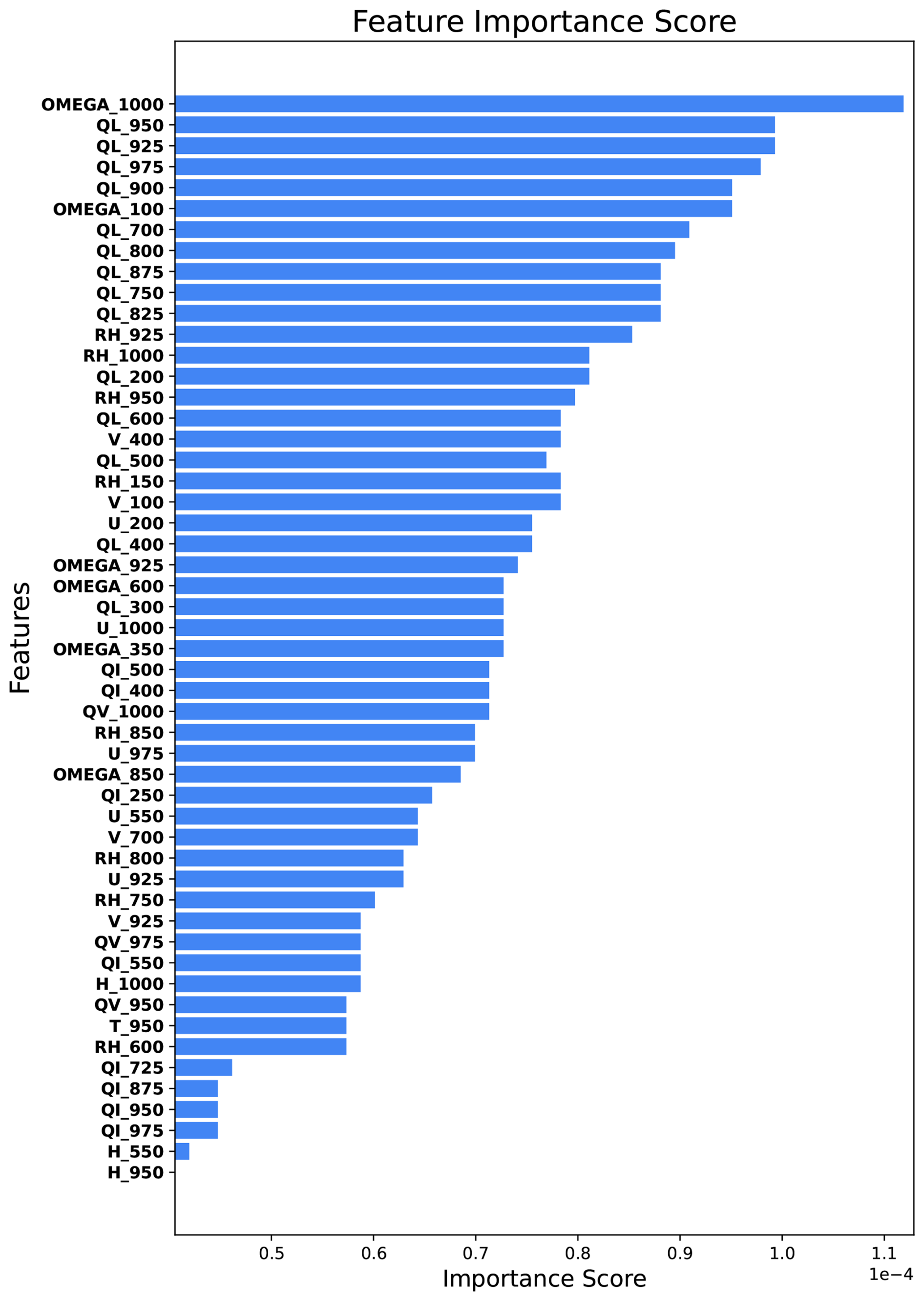
Figure 10 Feature-importance weights of the top-10 % features in the TCG-Net model for the Dynamic Domain task.

Table 5 compares the channels obtained from the two feature selection methods, using the MERRA-2 data during the training with the PD and DD strategies as shown in Figs. 9–10. It is of interest to note that the selected features between these two methods share a great number of overlaps, indicating that previous findings on TCG factors such as vertical wind shear (zonal wind components at 800 and 200 hPa level), low-level moisture (900–700 hPa relative humidity, RH), mid-level vertical motion (OMEGA at 500 hPa), or low-to-mid level temperature all play an important role in TCG prediction.

In addition to these common features, we notice that feature ranking appears to capture more pressure levels than feature engineering. For example, NK2024's feature engineering uses RH at 750 hPa, while feature ranking captures several levels for the DD strategy (see last column in Table 5). Likewise, zonal wind components in feature engineering require only 200 and 800 hPa, but feature ranking captures a group of levels at 1000, 550, 200 hPa. Despite this difference in the pressure levels, the fact that both feature engineering and feature ranking share many common features could indicate that ResNet-18 is capable of learning large-scale environments correctly for the TCG problem. From this regard, our DL model not only justifies the use of the feature engineering method in previous studies, but also presents a way to help enhance our understanding of the key environments governing TCG when the ranking is expanded to include more environmental factors.

Among all selected features, we should note that there are several features from the feature ranking method that are not included in feature engineering such as the specific liquid (QL) and ice content (QI), which represent the cloud information. In their early study, NK2024 did not include these features as they are linked to vertical motion and relative humidity via the CAPE channel. Similarly, the specific humidity (QV) is just an equivalent representation of RH and so it is not included in feature engineering. These variables, however, emerge from the output of feature ranking, probably because of their stronger roles in capturing TCG during the model training, even though they do not provide any new physical implications. Note also that the original MERRA-2 data does not contain some fields such as vorticity or divergence used in NK2024. Thus, several features in NK2024's study cannot be obtained from the ranking feature method shown in Table 5.

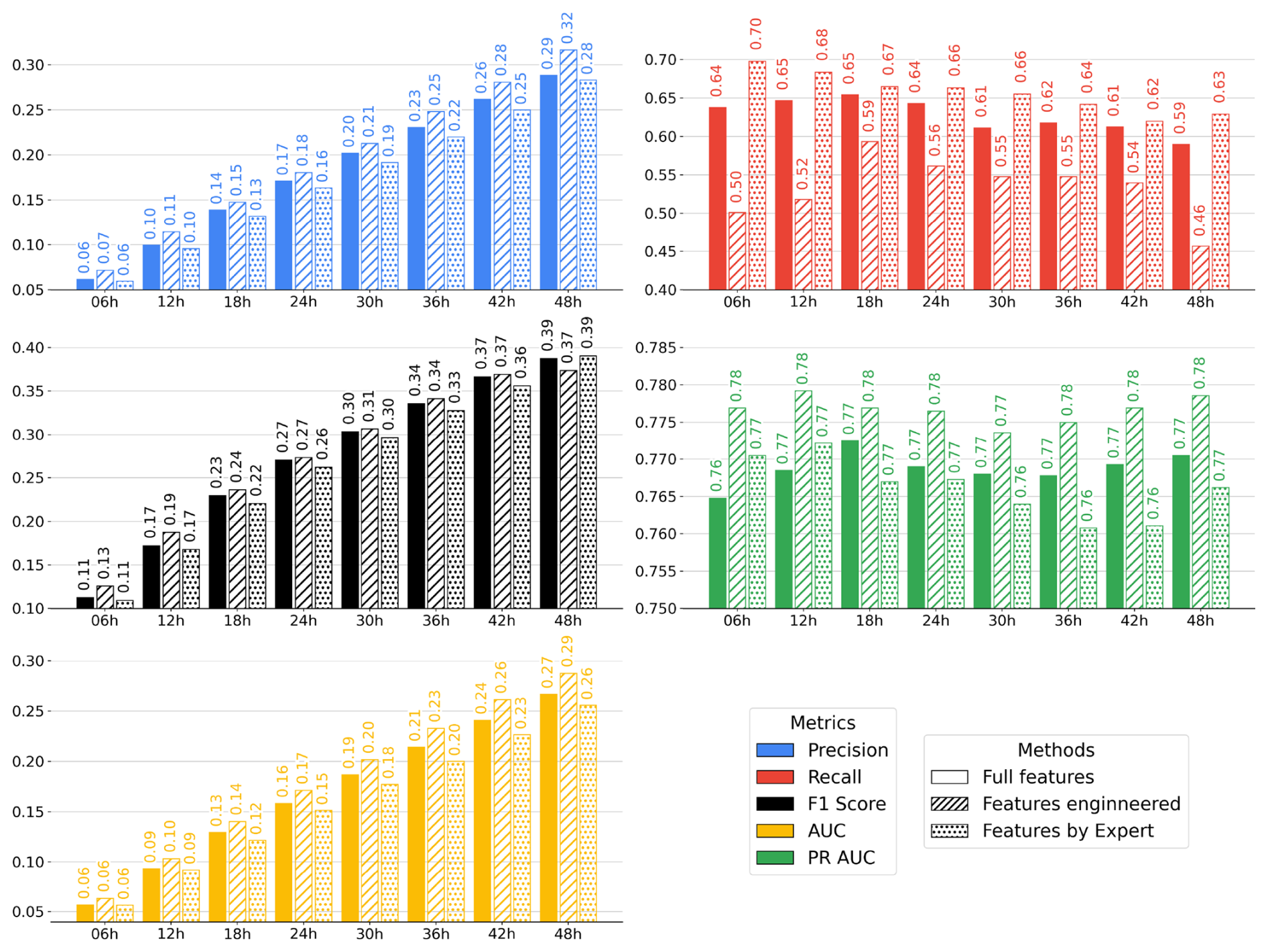
Figure 11 Evaluation of the model performance for several different feature selection methods including all features (solid color columns), 13 selected features based on feature engineering in Nguyen and Kieu (2024) (striped columns), and feature ranking of top 10 % (dotted columns) using the Past Domain task.

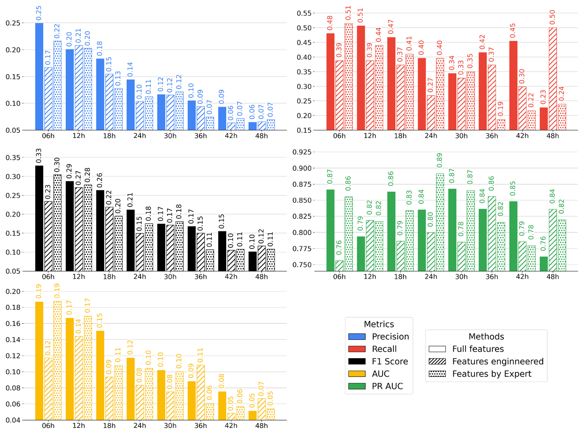
Figure 12 Evaluation of the model performance for several different feature selection methods including all features (solid color columns), 13 selected features based on feature engineering in Nguyen and Kieu (2024) (striped columns), and feature ranking of top 10% (dotted columns) using the Dynamic Domain task.

For model performance, Figs. 11–12 compare the F₁, P, and R scores among the full-feature, feature engineering, and feature ranking methods for both PD and DD labeling strategies. Among these feature selection methods, the feature ranking appears to deliver the most stable and effective results for the PD labeling strategy, particularly for long enrichment windows. The feature engineering and full-feature methods also perform well, but with slightly lower overall performance than feature engineering.

In contrast, the DD labeling strategy shows a declining trend in performance of the feature engineering method, with P,R and F₁ score all decreased over longer time windows. However, feature engineering still maintains relatively higher and more stable R values, indicating its potential utility in capturing more relevant signals in predicting TCG spatial distribution without the need of all data channels.

Regardless of the labeling strategy, one can see that both feature engineering and feature ranking provide similar performance for a range of data enrichment windows, despite much fewer features than the full-feature method. For a long window of 36–48 h, feature engineering and feature ranking could deliver even better performance for the PD approach, thus confirming that detecting TCG would mostly rely on a subset of variables/channels instead of full data at all levels. In fact, examining the spatial distributions of TCG climatology from both feature engineering and feature ranking (Figs. 13–14) shows little change in the overall patterns as compared to the full-feature output (cf. Fig. 6). The consistency among all feature selection methods is also captured for the seasonal TCG density (not shown), thus giving us some foundation for further understanding and predicting TCG based on a set of selected features for future DL improvement or implementations.

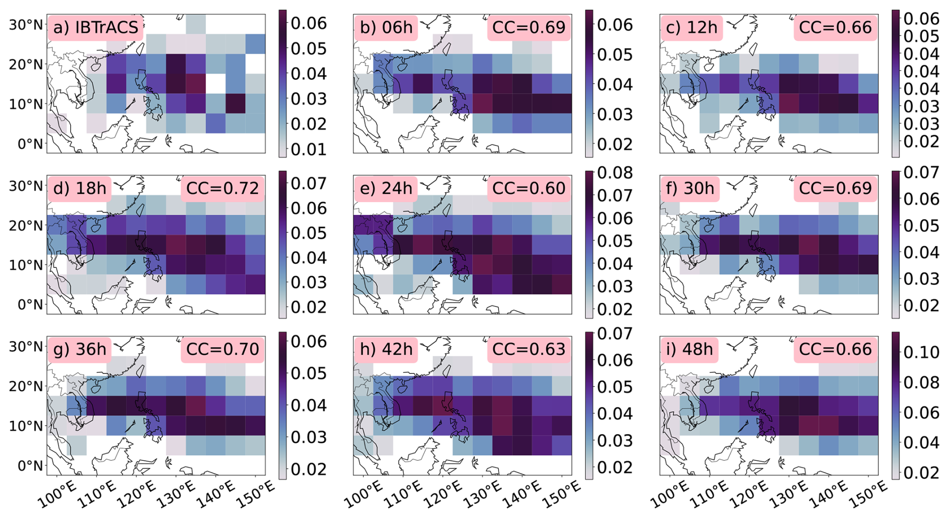
Figure 13 Similar to Fig. 6 but for the feature engineering approach.

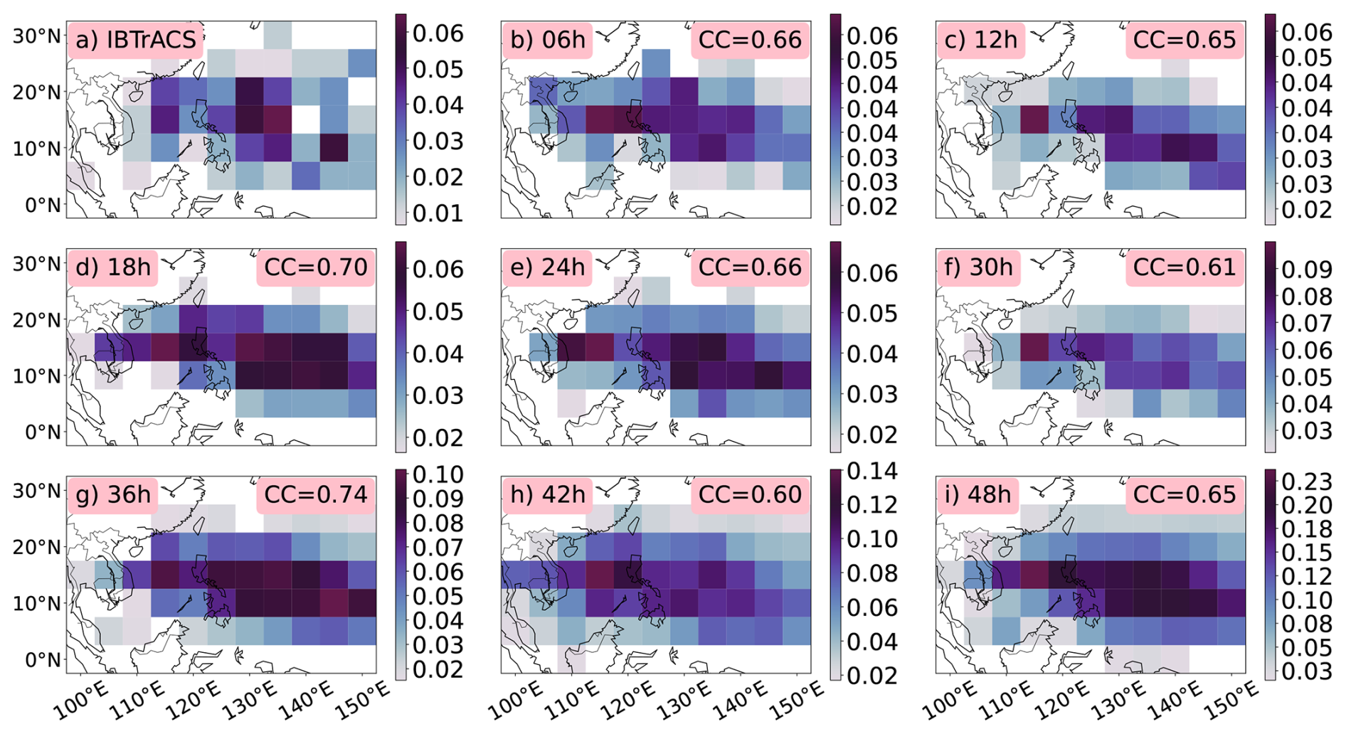
Figure 14 Similar to Fig. 6 but for the automatic feature ranking approach.

5 Conclusions

In this study, we presented a deep learning (DL) framework to reconstruct the climatology of tropical cyclone genesis (TCG) from climate reanalysis datasets. Recognizing that the definition of TCG climatology may vary depending on specific purposes and practical needs, our DL approach was designed and evaluated from multiple perspectives, based on different TCG labeling strategies for model training. Due to the limited number of TCG events available for training, we also implemented different data enrichment and feature selection methods to optimize our DL model for both TCG climatology reconstruction and potential prediction tasks.

Using the MERRA-2 reanalysis for the training data and the ResNet-18 architecture as a backbone for our DL model, we demonstrated that ResNet-18 exhibits promising capability in detecting TCG from climate data at 0.5° resolution. Although the F₁ score for TCG prediction remains relatively low, which is partly due to the inherent low predictability of TCG, the limited TCG samples, and related information available in MERRA-2, we showed that the F₁ score can be improved through appropriate hyperparameter tuning, labeling strategies, class weighting, and feature selections.

Comparing the DL-reconstructed seasonality and spatial distribution of TCG to the best track during the test period showed several noteworthy results. First, our ResNet-18 design could reproduce the seasonality of TCG monthly frequency, with double peaks of TCG frequency in August and October as well as the inactive period from January to May, consistent with those obtained from observations. Second, ResNet-18 could recover also the spatial distribution of TCG climatology, with main areas in the Eastern Philippine Sea and SCS. While there are some fluctuations in the TCG distribution for the areas along the coastal regions or different test periods Kieu et al. (2025), the overall well-recovered map of TCG in the WNP basin indicates that large-scale environments from the MERRA-2 dataset contain some important hidden signals of TCG processes that DL models can be trained and learn.

Further sensitivity experiments with different feature selection methods revealed that reconstructing TCG climatology from reanalysis datasets is possible due to the existence of some key channels that contain the required TCG signals for DL models to learn. Specifically, our use of feature engineering based on a set of features reported in previous studies and feature ranking that filters input features based on the model impacts both capture some common data channels needed for TCG processes. Several of these key features obtained from the MERRA-2 dataset are robust among sensitivity experiments, which include vertical wind shear, low-to-mid level moisture, mid-level vertical motion, or mid-level geopotential height. The feature ranking method could detect some additional features such as high-level liquid or ice content that may contain some cloud signal information beyond what used in previous models.

The results from these feature-sensitivity experiments support that combining expert knowledge with automated feature engineering can help enhance feature representation when training data is not sufficient, or when using full feature for DL model development is too costly. Moreover, while feature engineering helps avoid overfitting and promotes interpretability, the feature ranking approach can help uncover hidden signals beyond what known from previous studies. For our TCG problem here, at least both the feature engineering and feature ranking approaches could share similar factors, which help build more confidence in using those input features to understand the variability of TCG climatology. Future improvements could involve integrating approaches using ranking mechanisms, attention-based models, or dimensionality reduction to retain a compact yet informative feature set for TCG prediction tasks.

Along with the focus on reconstructing TCG climatology, this study suggests that our approach could hold some potential for real-time TCG prediction in operational settings. Depending on a specific forecasting objective, such as predicting TCG at a fixed location (as in the PD labeling strategy) or deriving the spatial distribution of TCG at any given time (as in the DD labeling strategy), a DL model can be designed and trained for each task separately. While the relatively low F₁ scores observed for both strategies indicate that real-time forecasts of TCG from climate or global model output is still considerably uncertain, our DL approach offers a valuable, independent alternative to traditional physical-based models, with the capability of providing early warnings of TCG 1–3 d in advance. In this context, our work contributes to a deeper understanding of TCG processes and offers another practical guidance for improving DL models in real-time applications, particularly for extreme events where minority classes are the main focus.

Despite promising capabilities, this study reveals also several key challenges in applying DL models to TCG research. First, DL performance is highly sensitive to data preprocessing methods, particularly in labeling negative TCG events, an issue that is exacerbated by the limited number of TCG occurrences. Second, the pronounced class imbalance between positive and negative TCG labels during training remains a significant barrier. Addressing this challenge requires a careful integration of undersampling techniques, data augmentation strategies, or dynamic class weighting to ensure more robust and consistent performance across evaluation metrics. Last, any model design and performance are strongly dependent on the training dataset, which make it hard to generalize from one resolution to the others. These challenges highlight the complexity of DL applications to extreme weather events that one needs to fully account for in any DL model development.