Process-oriented evaluation of quasi-stationary Rossby waves and their impact on surface air temperature extremes in dynamical downscaling over North America

Quasi-stationary Rossby waves are a crucial component of the general circulation and play a significant role in regional water and energy cycles, as well as in extreme events. However, process-oriented evaluation for Rossby waves is rarely performed for dynamical downscaling simulations. To close this gap, we evaluate three classes of dynamical downscaling approaches, with a focus on quasi-stationary Rossby waves and their impact on surface air temperature over North America during Northern Hemisphere summer. The three classes of models differ in the way large-scale forcing is provided: a limited-area model (LAM) constrained only by lateral boundary conditions, represented by RegCM4 from the North American branch of the Coordinated Regional Downscaling Experiment (NA-CORDEX), a LAM with spectral nudging to maintain consistency in large-scale dynamics with the forcing data, represented by the Weather Research and Forecasting (WRF) model simulation in NA-CORDEX, and a global variable-resolution model with smoothly varying grid spacings, represented by the Community Atmosphere Model version 5.4, with the Model for Prediction Across Scales (MPAS) as its dynamical core (CAM-MPAS). With no constraints on the atmospheric dynamics, CAM-MPAS exhibits several mean biases in the upper-level circulations over the Pacific Coast region: a weaker subtropical jet, a northward-shifted mid-latitude jet, and an overestimated southerly flow. With the lateral boundary constraint alone, RegCM4 also exhibits weaker jets and overestimated southerly winds off the West Coast. Rossby ray theory reveals that those wind biases direct incoming Rossby waves northward. The erroneously routed Rossby waves distort the relationship between the accumulation of wave activity over the US West Coast and surface temperature anomalies over the Southern Great Plains, which emerges approximately 4 d after the convergence of wave-activity flux in the ERA-Interim reanalysis. Furthermore, the response of heatwaves to the extreme wave activity flux is not reproduced by the two models, a serious drawback as a dynamical downscaling framework is expected to connect large-scale forcing to local-scale phenomena. The WRF model employing spectral nudging is largely free from the aforementioned problems. A pair of sensitivity simulations suggests that spectral nudging is the key to improving the dynamics of quasi-stationary Rossby waves and their impact on surface air temperature. Our results also demonstrate the effectiveness of Rossby wave diagnostics that allow for realistic background flows for assessing the credibility of dynamical downscaling over North America, where incoming Rossby waves propagate through complex circulation patterns before traveling across the continent.

1 Introduction

Rossby waves have the largest spatial scales among the atmospheric waves (1000–10 000 km). Their spatial extent makes it possible to connect tropical convection to mid-latitude weather (Wallace and Gutzler, 1981; Ambrizzi et al., 1995; Branstator, 2014). Rossby waves can be “quasi-stationary” by having a phase speed nearly equal to the background winds but in the opposite direction, thus their phase (maxima and minima) becomes fixed in space. Some large waves become quasi-stationary even within the atmospheric jet streams, where vorticity gradients and strong winds can trap and help the waves travel further (Manola et al., 2013; Branstator and Teng, 2017; Wirth, 2020). Such large, (quasi-)stationary Rossby waves are one of the important drivers for regional climate because their associated momentum and energy fluxes modify regional circulation and atmospheric stability (e.g., Weaver and Nigam, 2008; Hoskins and Woollings, 2015; Teng and Branstator, 2017, 2019; Wills et al., 2019; White et al., 2022). Rigorous evaluations of simulated Rossby waves are thus necessary for establishing confidence in regional climate projections. To this end, this study revisits and evaluates the large-scale circulations relevant to Rossby wave propagation to North America, as well as the physical connection between quasi-stationary Rossby waves and regional climate, specifically near-surface air temperature (tas).

The heatwave over the Pacific Northwest (PNW) in July 2009 is a good example of a relationship between quasi-stationary Rossby waves and tas anomaly. This event marked the highest maximum temperature in the record across the region (Bumbaco et al., 2013), until it was exceeded by a more recent heatwave in 2021 (White et al., 2023), which falls outside our study period. A spatiotemporal correlation between the upper-level geopotential height anomaly and the daily tas anomaly is evident during this month (Fig. 1d–i). Figure 1a–c illustrate the flux of wave activity (WA), second-order variability of wind fields associated with Rossby waves (Takaya and Nakamura, 2001) (hereafter TN01). The WA flux delineates the flux of perturbation geopotential height in the direction of the group velocity, which is also associated with a negative momentum transport for the mean circulation (Takaya and Nakamura, 2001, section 4). In other words, ahead of the WA convergence, one sees an increase in the perturbation geopotential height and a reduction in mean wind speeds. The region behind the WA divergence experiences a decrease in perturbation geopotential height and an acceleration of the mean winds.

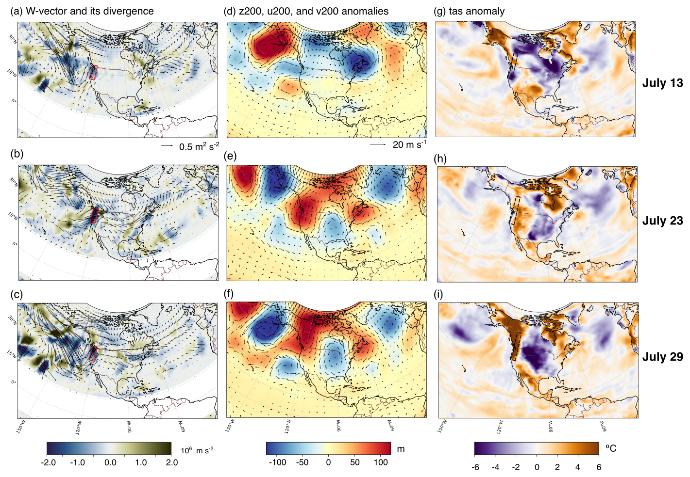
Figure 1 Evolution of quasi-stationary Rossby waves and surface air temperature (tas) during the 2009 heatwave event: (a–c) the flux (arrows) and divergence (color, blue = convergence, green = divergence) of daily-mean wave activity (WA) flux derived from the 25–90 d band-passed geopotential height anomalies, (d–f) 200 hPa winds and geopotential height anomalies (25–90 d band-passed), and (g–i) daily tas anomaly, all variables from ERA-Interim.

About two weeks before the most intense heatwave on 29 July, the PNW region was under a weakly negative height anomaly (Fig. 1d), but the WA flux had already started converging over the region (Fig. 1a). The flux is dominantly meridionally oriented, flowing out northward from the subtropical eastern Pacific, where intense wave activity flux has been converging from the mid-latitude North Pacific. Some WA flux appears to originate from the tropical east Pacific region as well. The WA flux convergence continued and became more intense over the next 10 d, during which a positive geopotential anomaly built up over the PNW region (Fig. 1b and e). In response, a positive tas anomaly has emerged (Fig. 1h). The WA flux convergence over the PNW continued, spreading the positive geopotential anomaly northward to cover Washington state in the United States and the entire Canadian West coast by 29 July (Fig. 1c and f), when a positive tas anomaly > 6 °C has extended over most of the PNW region (Fig. 1i). The effect of WA flux divergence through geopotential changes to tas appears to take approximately 6 d based on the lead/lag correlation. Figure A1a shows that the linear correlation reaches a maximum value of 0.56 at a negative lag of 6 d applied to the WA flux divergence. The evolution of the upper-level geopotential height anomalies follows the typical condition during heatwave events over the region, with the high anomaly centered over Vancouver Island near the Canada–US border (Fig. 1e and f) (Bumbaco et al., 2013). This circulation structure is a part of the East Pacific–North Pacific pattern that is characterized by a southward-shifted and more intense jet across the Pacific (Bell and Janowiak, 1995).

The 2009 heatwave is just one example; significant connections between quasi-stationary Rossby waves and regional climate and extreme events have long been suggested. Analyzing 30 years of reanalysis data, Schubert et al. (2011) found that meridional wind variabilities associated with stationary Rossby waves account for up to 60 % of surface temperature variabilities over large areas in North America. Teng et al. (2013) found that stationary waves with zonal wavenumber-5 patterns often appear 15–20 d before heatwave events in the United States in 12 000 years of atmospheric general circulation model (GCM) simulations. Yuan et al. (2015) investigated the variability and trend of subtropical stationary waves during the NH summer. They found an increasing trend in wave amplitude over the 1979–2013 period, as well as changes in regional moisture fluxes associated with stationary waves that affected hydroclimate across several regions, including the central United States. In recent decades, an increasing number of studies have investigated how quasi-stationary waves contribute to extreme events (Coumou et al., 2014; Hoskins and Woollings, 2015; Kornhuber et al., 2017; Wolf et al., 2018).

Due to the significance of (quasi-)stationary waves on regional climate, several recent studies have evaluated Rossby waves in GCM simulations and further found connections between the model's skills in simulating Rossby waves and in simulating the surface climate (e.g., Holman et al., 2014; Luo et al., 2022). For example, Simpson et al. (2020) used standard performance metrics, such as spatial correlation and root-mean-square errors of the time-mean eddy streamfunction, to evaluate stationary Rossby waves in two generations of model ensembles from the Coupled Model Intercomparison Project (CMIP) and a large ensemble of a single model. They found improved performance from the CMIP phase 5 (CMIP5) to CMIP6, and the model biases tend to be larger in JJA than in DJF. Other studies used metrics derived from linear wave theory and the vorticity budget to evaluate simulated Rossby waves. Nie et al. (2019) evaluated Rossby wave sources in the CMIP5 models, and Henderson et al. (2017) evaluated the teleconnection between North America and Madden-Julian Oscillation using the so-called stationary wavenumbers. Some studies have taken a step further to use more complex diagnostics of Rossby waves, such as the WA flux and Rossby wave ray tracing, to find close connections between near-surface climate and Rossby wave propagation biases in GCMs (Garfinkel et al., 2022; Choi and Stan, 2024). However, few studies have evaluated large-scale stationary Rossby waves in regional, dynamical downscaling simulations.

For limited-area models (LAMs), previous studies have focused on atmospheric circulations with spatiotemporal scales smaller than those of quasi-stationary Rossby waves. Using the “Big-Brother Experiment” in which a smaller domain simulation is forced by the output from the larger-domain simulation using the same model, Denis et al. (2002b), Denis et al. (2003), and Dimitrijevic and Laprise (2005) evaluated the simulated atmospheric circulations on a monthly time scale. These studies found that lateral boundaries (LBs) do not significantly affect modeled sea-level pressure and relative vorticity; however, the vorticity fields exhibit some deviations from the driving model at higher atmospheric levels. Using a similar experimental design but with an idealized dry test case, Park et al. (2014) found unphysical inertia-gravity waves excited at the LBs. The artificial waves become stronger with longer LB update time periods, particularly when they are substantially longer than the LAM timestep, which is usually the case in climate-scale model integration. Miguez-Macho et al. (2004) documented how the interactions between the simulated flow and specified flows at LBs distort large-scale circulations in regional simulations over North America, and also demonstrated the usefulness of spectral nudging for the waves with synoptic and larger scales to remove the large-scale flow biases. Imberger et al. (2020) investigated the impact of the LB update frequency, size of the LB relaxation zone, and spectral nudging in the case study of a fast-propagating, strong mid-latitude storm. They found that the update frequency is most effective in mitigating reductions in storm intensity through LBs. Castro et al. (2007) and Chang et al. (2015) investigated how the modes of large-scale climate variabilities via Rossby waves are simulated in regional downscaling by Empirical Orthogonal Functions, focusing on the teleconnections between tropical sea surface temperature (SST) and the North American Monsoon. They found that spectral nudging helps reproduce large-scale climate variabilities, but the dynamics and kinematics of Rossby waves were not their focus. Scarcity of Rossby wave evaluation in regional simulations may be related to an assumption that the large spatiotemporal scales of quasi-stationary Rossby waves are well resolved by the host GCM grid and sub-daily (e.g., six-hourly) frequency updates of LB conditions. However, this assumption is not necessarily valid.

A common numerical treatment of LB conditions is to blend the specified forcing with the state simulated by LAMs (e.g., Davies, 1976). Staniforth (1997) noted that such blending does not retain the balance within the flow, such as geostrophy. Deviation from the geostrophic balance excites inertia-gravity waves to restore the balance (Holton, 2004). The excitation of inertia-gravity waves would bring the state closer to geostrophic balance, but the LB treatment occurs at every time step; thus, the vicinity of the boundaries may always experience artificial imbalance. Such a disruption would distort the propagation of incoming Rossby waves, and the persistent divergence produced by the unphysical inertia-gravity waves (Park et al., 2014) may also contaminate the amplitude of the incoming Rossby waves.

Another modeling framework for dynamical downscaling is global variable-resolution (VR) models. One such model, the Model for Prediction Across Scales (MPAS, Skamarock et al., 2012), is developed on an unstructured grid that can smoothly change grid spacing over a specified region. This model has been shown not to have the aforementioned issues associated with LBs (Park et al., 2014). However, the amplitude, pathways, and frequency of Rossby waves arriving in North America may be unrealistic. This is because for those waves originating from the tropics, the strength and spatial scales of the wave source are linked to the amplitude and profile of diabatic heating in the organized tropical convection, which is known to be difficult for GCMs to realistically simulate (Dai, 2006; Bacmeister et al., 2014; Bogenschutz et al., 2018; Park and Lee, 2021; Zhou et al., 2022; Chang et al., 2025). Furthermore, GCMs have long-standing biases in the location and strength of the jet (Harvey et al., 2020; Simpson et al., 2020). For dynamical downscaling using LAMs, one can choose host GCMs with small biases in those aspects. For dynamical downscaling with a global VR model, the model must exhibit good skills in both global-scale and regional-scale processes.

There is thus a clear need to evaluate quasi-stationary Rossby waves in dynamical downscaling simulations; however, a process-oriented evaluation has not been conducted to assess how different modeling frameworks simulate them. To fill this gap, we evaluate three classes of dynamical downscaling approaches that have distinct representations of large-scale forcing. The first class is a standard regional climate simulation with a LAM, represented by the Regional Climate Model version 4 (RegCM4) simulation available from the North American branch of the Coordinated Regional Downscaling Experiment (Mearns et al., 2017) (NA-CORDEX). The second class is also an LAM simulation, but employs spectral nudging to constrain large-scale atmospheric dynamics; the WRF simulation in NA-CORDEX is one such dataset. The third class is a global VR model that utilizes the MPAS dynamical core within the Community Atmosphere Model (CAM), referred to as CAM-MPAS. This model's regional refinement and simulation design follow the NA-CORDEX protocol (Sakaguchi et al., 2023). We will demonstrate that these three classes of models exhibit distinct biases in the upper-level circulations and Rossby wave propagations. We also provide reviews and technical details of the diagnostics throughout the text and in the appendices for those interested in more background on Rossby wave theory.

2 Data and methods

2.1 Downscaling and evaluation dataset

We use two simulations from the “Evaluation” experiment in NA-CORDEX (Diez-Sierra et al., 2022a), one using the RegCM4 model and the other using the WRF model. Both models are configured on 25 km grids following the NA-CORDEX protocol (Fig. 2b) (Diez-Sierra et al., 2022b). We also analyze another downscaling simulation conducted with the CAM-MPAS model on a global VR grid with a 100 km coarse domain refined smoothly to 25 km grid spacing over North America (Fig. 2a).

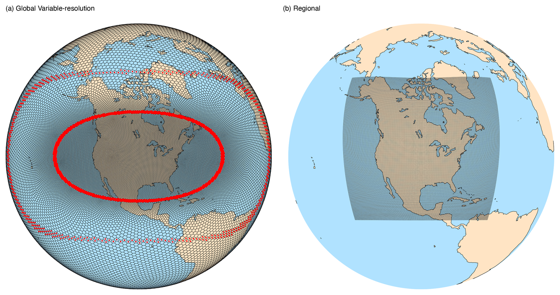
Figure 2 Model mesh examples: (a) global variable-resolution mesh for CAM-MPAS, (b) regional mesh for WRF. The mesh used by RegCM4 is visually similar to that of WRF (hence not shown), except it covers a slightly larger area.

The RegCM model is a widely used regional climate model with a long history (Giorgi and Anyah, 2012). Downscaled data from the fourth-generation RegCM4 are available from NA-CORDEX on both the 50 and 25 km grids (Mearns et al., 2017; Bukovsky and Mearns, 2020; McGinnis and Mearns, 2021). This model version solves the primitive (hydrostatic) equations on a σ coordinate as described in Grell et al. (1994) and Elguindi et al. (2017). Multiple options are available for the cumulus, boundary layer, and land-surface components (Giorgi et al., 2012). The physics parameterizations were selected based on the performance of test simulations over the CONUS region, particularly for warm-season precipitation (Raymond W. Arritt and Melissa S. Bukovsky, personal communication, 2018).

The WRF model is a regional model for weather and climate applications (Skamarock et al., 2008) and has been extensively used to study the present-day and future state of North American climate with a wide range of model resolutions and configurations (e.g., Chang et al., 2015; Liu et al., 2017; Chen et al., 2019; Srivastava et al., 2023). Version 3.5.1 was used for the NA-CORDEX experiment (50 and 25 km). The dynamical core solves the Euler equations without the hydrostatic assumption. The model physics largely follows that of Castro et al. (2012), who focused on the warm-season climate of the western CONUS and the North American monsoon. Spectral nudging is applied to the temperature, winds, and geopotential height fields at the scales larger than approximately 1000 km to retain synoptic-scale variability in the driving GCM or reanalysis data (Castro et al., 2005, 2012; Hu et al., 2018).

CAM-MPAS is an experimental model in which the dynamical core is ported from the MPAS-Atmosphere version 4 to the CAM model within a beta version of the CESM2. The technical description of the model and downscaling experiments are provided in Sakaguchi et al. (2023). Briefly, MPAS is a global dynamical core that solves the Euler equations on an unstructured grid (Skamarock et al., 2012). The unstructured grid can be configured as a global quasi-uniform resolution grid or a VR grid, in which one or more regions of interest have finer grid spacing than the rest of the globe. Advantages of the global VR model over LAMs include the absence of LBs and the consistent dynamical and physical schemes in both the high-resolution (downscaling) and coarse-resolution domains, which can avoid artificial shocks or gradients created by LBs in LAMs.

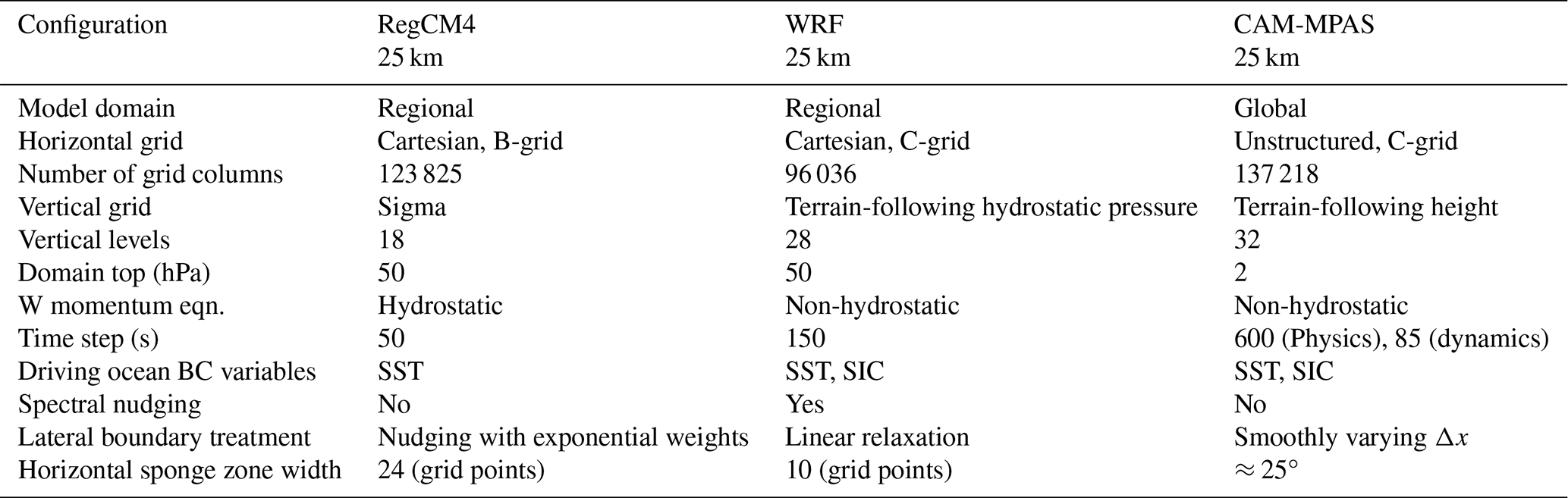
All models use the ERA-Interim reanalysis product for initial and boundary conditions, including six-hourly updates to the LBs and daily updates to SST and sea ice fraction (SIC) at the bottom (surface) boundary. RegCM4 does not have a specific sea ice scheme, so SIC from ERA-Interim is not used. CAM-MPAS uses SST and SIC only since there are no lateral boundaries; therefore, the large-scale circulations are not constrained. Table 1 lists the model characteristics and configurations. Table B1 compares the physics parameterizations used by the three models.

Table 1 Characteristics of the three downscaling models. The sponge zone width in CAM-MPAS refers to the transition zone. All models solve compressible mass and momentum equations. SST: sea surface temperature, SIC: sea ice fraction.

The reference data we use is ERA-Interim, which drives the NA-CORDEX simulations for the “Evaluation” experiment. As discussed by Laprise et al. (2008), we expect that dynamical downscaling adds value primarily in the small-scale processes while maintaining the large-scale flow provided from the driving data. If this tenet is true, incoming Rossby wave signals are not affected by LBs or other model details (see Appendix B1); Rossby wave metrics calculated from the driving data (ERA-Interim) and from downscaling simulations within the LAM domain should be very close to each other. On the other hand, if numerical aspects of the downscaling model affect the circulations, such as artificial sources of divergence over the time scale of quasi-stationary Rossby waves, or the model exhibits mean biases in the general circulations (e.g., jet strength/width/positions), then we would see deviations in the Rossby waves between the driving data and the downscaling simulations. We are aware that this logic ignores a potential upscale effect from the downscaling simulation on the quasi-stationary Rossby waves. We will briefly discuss this assumption in Sect. 4; however, such upscaling signals cannot be easily quantified without a priori designed experiments (e.g., Denis et al., 2002b; Leung et al., 2013; Sakaguchi et al., 2016), and this is left for future work.

2.2 Data preparation

The NH summer season (JJA) in the 30-year period from 1980 to 2010 is analyzed, except for the CAM-MPAS simulation, which starts at 1990. Most analyses are performed using daily-mean variables at 200 hPa (zonal and meridional winds, geopotential height). This particular pressure level is chosen primarily because it is a standard pressure level available in the CORDEX archives (CORDEX, 2009). According to the CORDEX protocol's model data requirements, daily mean quantities are calculated from three-hourly data (CORDEX, 2009). The CAM-MPAS data follow this requirement. The ERA-Interim data is available only every six hours, from which we calculated daily statistics. We compared the seasonal means and standard deviations of the monthly mean tas calculated from the six-hourly and three-hourly data, and found that the differences in these statistics are significantly smaller (less than 10 %) than the model biases against ERA-Interim (not shown).

Grid boxes adjacent to the LBs, or “sponge/buffer/relaxation zone”, where the external forcing and model-predicted variables are blended (Table 1, Appendix B1), have already been removed in the NA-CORDEX data. This post-processing is designed for the common use case of regional climate assessment within the model domain; for this study, it poses a challenge. This is because we patch the outside of the LAM domain with ERA-Interim data to produce spatially continuous fields, on which Rossby wave propagations are diagnosed. Without the relaxation zone that blends LAMs predictions and ERA-Interim data, our patched diagnostic approach exhibits stronger gradients between the model and ERA-Interim data than with the relaxation zone. We used a brief WRF simulation to evaluate the impact of removing the buffer zone, which was found not to significantly alter the analysis results within the model domain (Fig. B2). However, within the blending zone, the strength and spatial pattern of derived quantities (e.g., vorticity, divergence, and WA fluxes) change, and overall, they are notably noisier without the blending zone (Fig. B2a, b, d and e). The noise and spurious WA fluxes can be reduced to some extent by spatial smoothing applied over the relaxation zone (Fig. B2c and f). We tested several smoothing methods and present the figures that utilized a Gaussian filter within the buffer zone when the noise is significant. We do not attempt to evaluate Rossby wave sources/sinks along the LBs; those crucial aspects will be assessed in future work.

Prior to the patched analyses, all the data are regridded to a global 0.7° latitude–longitude grid using the patch method available from the Earth System Modeling Framework (ESMF) library (Balaji et al., 2018). The 0.7° grid is nearly identical to the original ERA-Interim grid and is coarser than the downscaling datasets. We still remap the ERA-Interim data to this grid to more fairly compare variability and extremes with the models, since remapping can smooth the fields and affect those statistics (Sakaguchi et al., 2023). The patch method first estimates the grid corner values on the source grid using the second-order polynomials, then weight-averages the corner values to obtain the final estimate on a target point value on the destination grid; therefore, the computation is more expensive than the commonly used bilinear method (Zienkiewicz and Zhu, 1995). The patch method estimates the values and their derivatives more accurately than the bilinear method (Balaji et al., 2018), which is desirable for calculating Rossby wave diagnostics that involve spatial derivatives.

It is critical to rotate the grid-relative u and v winds to the Earth-relative (eastward and northward) winds in the RegCM4 and WRF data before regridding. For the WRF model, the NCAR Command Language (NCL: NCAR, 2017) provides a function for wind rotation (wrf_uvmet). For RegCM4, we wrote an NCL function to rotate winds onto the Rotated Mercator projection, which is available in Sakaguchi (2025). It is often necessary to spatially smooth the variables, especially for winds at relatively high resolution. In most cases, we used a suite of spherical harmonic functions available in NCL: vhaeC, tri_trunC, and shaeC.

2.3 Diagnostic framework

2.3.1 Rossby wave ray theory

Wirth et al. (2018) reviewed diagnostics to study the dynamics of Rossby waves, particularly the frameworks to identify and track so-called Rossby wave packets. Wave energy, momentum, and other information propagate with the wave packets at the group velocity, not with individual wave crests/troughs (Vallis, 2017, Chap. 6). One commonly used diagnostic is ray theory, which traces the trajectory of a wave packet from a specified source location. The potential or absolute vorticity equations are linearized by decomposing the variables into the base state (or background or reference state), which does not vary in time during the lifetime of the wave packet, and the perturbation from the base state (wave motions). Assuming a wave-like solution to the linearized equation and scale separation between the wave motion (small) and base state (large), we can obtain an algebraic relationship among the wave frequency, wavenumbers, and base states (the wave dispersion relationship) at a given location. Further assuming that the base state varies much more slowly than the waves do, we can get a set of ordinary differential equations for the time evolution of the wavenumbers and frequency. Combining these kinematic and dynamic relationships, we can predict where the wave packets will travel from the source at t=0 to another location at t=1. At the new location, we solve for the wavenumbers again with the new environmental conditions, yielding a new group velocity. Repeating the process gives us the evolution of wavenumbers and group velocities across space and time (Li et al., 2015). Vallis (2017) provides a general introduction to ray theory for Rossby waves.

Hoskins and Karoly (1981) first applied the ray theory (Whitham, 1960) to quasi-stationary Rossby waves. Their ray theory assumes that the meridional wind in the base state ($\stackrel{\mathrm{‾}}{v}$) is zero, and the zonal wind ($\stackrel{\mathrm{‾}}{u}$) is a function of latitude only. Despite these strong assumptions, their result reproduced many aspects of the Rossby wave propagations inferred from statistical analyses and numerical model results. However, this assumption is difficult to justify given our focus on regional climate over North America, as seen in the 2009 heatwave example in the Introduction. Karoly (1983) applied the ray theory to a base state that varies in both the zonal and meridional directions, with non-zero $\stackrel{\mathrm{‾}}{u}$ and $\stackrel{\mathrm{‾}}{v}$. Their work was extended by Li et al. (2015) and Zhao et al. (2015) (hereafter LZ2015), which is adopted in our analysis. The input for the LZ2015 ray theory consists of the wave source location, the initial zonal wavenumber k₀, and the background winds in the Mercator projection $({\stackrel{\mathrm{‾}}{u}}_{\mathrm{M}},{\stackrel{\mathrm{‾}}{v}}_{\mathrm{M}})=(\stackrel{\mathrm{‾}}{u},\stackrel{\mathrm{‾}}{v})/\cos \left(\mathit{\phi }\right)$ where φ is latitude. Given those inputs, LZ2015 solves the following equations (Eqs. 11 and 12 in Li et al., 2015):

$$\begin{array}{}\text{(1)}& {\displaystyle }{\displaystyle \frac{{\mathrm{d}}_{\mathrm{g}}k}{\mathrm{d}T}}=-k{\displaystyle \frac{\partial {\stackrel{\mathrm{‾}}{u}}_{\mathrm{M}}}{\partial X}}-l{\displaystyle \frac{\partial {\stackrel{\mathrm{‾}}{v}}_{\mathrm{M}}}{\partial X}}-{\displaystyle \frac{\mathrm{1}}{K^{\mathrm{2}}}}\left(l{\displaystyle \frac{\partial {\stackrel{\mathrm{‾}}{\mathit{\eta }}}_x}{\partial X}}-k{\displaystyle \frac{\partial {\stackrel{\mathrm{‾}}{\mathit{\eta }}}_y}{\partial X}}\right)\text{(2)}& {\displaystyle }{\displaystyle \frac{{\mathrm{d}}_{\mathrm{g}}l}{\mathrm{d}T}}=-k{\displaystyle \frac{\partial {\stackrel{\mathrm{‾}}{u}}_{\mathrm{M}}}{\partial Y}}-l{\displaystyle \frac{\partial {\stackrel{\mathrm{‾}}{v}}_{\mathrm{M}}}{\partial Y}}-{\displaystyle \frac{\mathrm{1}}{K^{\mathrm{2}}}}\left(l{\displaystyle \frac{\partial {\stackrel{\mathrm{‾}}{\mathit{\eta }}}_x}{\partial Y}}-k{\displaystyle \frac{\partial {\stackrel{\mathrm{‾}}{\mathit{\eta }}}_y}{\partial Y}}\right)\end{array}$$

where k and l are the zonal and meridional wavenumbers (m⁻¹), $K=\sqrt{k^{\mathrm{2}}+l^{\mathrm{2}}}$ is the total wavenumber, $\stackrel{\mathrm{‾}}{\mathit{\eta }}$ denotes the background absolute vorticity (s⁻¹), $\stackrel{\mathrm{‾}}{\mathit{\eta }}=\stackrel{\mathrm{‾}}{\mathit{\zeta }}+f$, f is the Coriolis parameter, and $\stackrel{\mathrm{‾}}{\mathit{\zeta }}$ is the vertical component of the background relative vorticity. The coordinate variables T, X, and Y are the time, zonal, and meridional coordinates for the mean state that has substantially larger scales than a local, wave-scale motion (t, x, y). Here, x=aλ and $y=\ln \left[\right(\mathrm{1}+\sin \mathit{\phi })/\cos \mathit{\phi }]$ in the Mercator projection. The operators ${\mathrm{d}}_{\mathrm{g}}/\mathrm{d}T=\partial /\partial T+u_{\mathrm{g}}\partial /\partial X+v_{\mathrm{g}}\partial /\partial Y$ represent the total derivative describing the rate of change following the wave packet moving at the group velocity (the subscript “g” denotes group, not geostrophic flow). Expressions for the group velocity are given in the Appendix C. To maintain consistency with the assumed scale separation, climatological mean fields are smoothed by truncating wavenumbers greater than 10 after spectral decomposition in spherical harmonics, before being passed to the ray-tracing algorithm. Also, to be consistent with our focus on quasi-stationary Rossby waves, the time frequency is set to zero for our analysis (see Eqs. C10 and C11).

After running the ray tracing algorithm, we can visually compare wave ray trajectories in the background state from ERA-Interim and those from the model simulations. To make model evaluation more quantitative than relying on visual inspection of rays, we compare the probabilities of Rossby wave propagation at each grid point, obtained by tracing a large number of rays. For example, if 5000 Rossby wave rays are initiated in a source region with slightly different input parameters, and 50 of them pass a grid box, then the probability of 0.01 is assigned to the grid box. To create an ensemble ray tracing, we start rays every two grid boxes within a source region (≈20 to 40° wide in the x and y directions), resulting in ≈150 to 300 source points per region. For each source point, we initiate Rossby waves with 12 different k₀ (1–12). We also consider three background states: the climatological winds for June, July, and August. Permuting the source points, 12 initial zonal wavenumbers, and three base states yields 5000 to 10 000 ray trajectories from each source region.

We note that this is a rather arbitrary approach to creating an ensemble of Rossby rays, since our base state and choice of k₀ may ignore important characteristics of Rossby waves in a particular region or time period. For instance, the preferred wavelengths of quasi-stationary waves excited over the Indian Monsoon region and the Tibetan Plateau appear to differ (wavenumbers 6–7 for the former and 4–5 for the latter; Joseph and Srinivasan, 1999; Park et al., 2013). To more accurately quantify the probabilities of ray trajectories beyond model evaluations, one may consider a broader range of parameter space (Li et al., 2019) and/or specify the parameter ranges based on a priori knowledge of the wave sources and time period of interest (Garfinkel et al., 2022; Chang et al., 2023a). Here, our tenet is that, given the same set of parameters and specifications for the base state, dynamical downscaling models can reproduce the probability distributions of quasi-stationary Rossby waves in the original forcing data if the relevant large-scale dynamics are faithfully retained.

2.3.2 Wave activity flux

In the introduction, we used the diagnostic derived by Takaya and Nakamura (1997, 2001) to visualize the WA flux, which is a linear combination of kinetic energy and enstrophy and is also related to the momentum and energy exchange between the mean circulation and perturbations. Similar to LZ15, TN01 used a horizontally non-uniform background with non-zero meridional winds to derive their WA budget equation, making it an appealing tool for regional climate studies (Schneidereit et al., 2012; Sakaguchi et al., 2016; Chen et al., 2023; Zhang et al., 2024). TN01 obtained the following conservation equation for WA from the quasi-geostrophic (QG) potential vorticity equation:

$$\begin{array}{}\text{(3)}& \begin{array}{rl}& {\displaystyle \frac{\partial M}{\partial t}}+\mathrm{\nabla }\cdot \mathit{W}=D_{\mathrm{T}}\\ & M={\displaystyle \frac{\mathrm{1}}{\mathrm{2}}}(A+E)\end{array}\end{array}$$

where M (m s⁻¹) is the wave activity density, W is WA flux (m² s⁻²), A and E are the quantities proportional to perturbation vorticity and kinetic energy, and D_T represents non-conservative diabatic and friction terms (m s⁻²). Since WA flux is denoted by W in TN01, we refer to their WA flux as the W-vector as well. All quantities are derived from the base-state and perturbation geopotential height. The actual expression for the W-vector is provided in the Appendix C3. The vertical components of the W-vector and the wave activity density are not included in the analysis. This is primarily because they involve vertical derivatives, but data at multiple pressure levels with sufficient resolution at a daily frequency are not always available from model archives such as NA-CORDEX. As a result, we infer the source/sink of WA by the convergence/divergence of the horizontal components of the W-vector. With the complexity of realistic atmospheric fields, it can be challenging to identify the climatological sources of WA at a given location; one would need to systematically pre-process the perturbations to decompose Rossby waves into different spatiotemporal scales, or use idealized numerical experiments.

In this study, we apply a 25–90 d frequency band-pass filter to the perturbation geopotential height to extract the quasi-stationary Rossby wave signals. The phase velocity is set to zero in the W-vector terms (Eq. C20). The base state is the 30-year (20-year for CAM-MPAS) daily climatology. The W-vector is calculated for each day and then averaged to produce the 30-year JJA climatology for visualization purposes. We noted that the result is insensitive to varying levels of spatial smoothing of the background state (not shown), presumably due to the underlying QG framework. Insensitivity to the background smoothness is an advantage for a diagnostic metric. On the other hand, the QG assumption appears to limit the validity of the W-vector in low-latitude regions, where we often observe unphysical variability in the W-vector.

The LZ15 ray theory predicts wave-ray propagation based on relationships between wave kinematics and the background state (e.g., how background wind shear changes wave shapes), given the specified initial conditions. It is applicable over the tropics and deals with a single wave packet from a specified location, making the source attribution straightforward. However, the barotropic, non-divergent vorticity equation underlying the LZ2015 does not consider an influence of divergence on Rossby wave propagation (Li, 2020), and the wave amplitude is not diagnosed. These two are included in the W-vector, which diagnoses the wave characteristics directly from the perturbation geopotential height. Therefore, TN01 (the W-vector) and LZ15 (wave-ray) diagnostics complement each other, enabling a better understanding of model biases in Rossby wave dynamics.

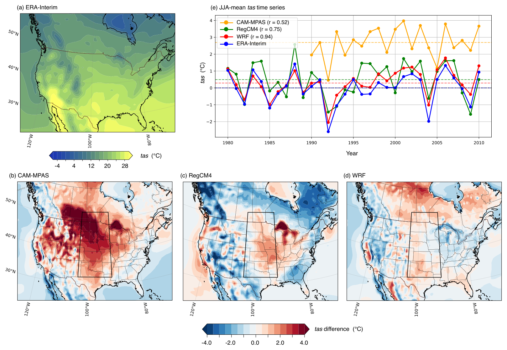
Figure 3 JJA-mean tas over North America in ERA-Interim (a) and tas difference between ERA-Interim and (b) CAM-MPAS, (c) RegCM4, and (d) WRF. The panel (e) shows the time series of JJA-mean tas anomaly in each year, averaged over the central North America (the black box in b–d). The mean bias against ERA-Interim is added to the anomaly time series and shown by the colored dashed lines. The legend text includes the linear correlation (r) between the model and the ERA-Interim time series.

3 Results

3.1 Evaluation of surface air temperature

We begin with the evaluation of tas in the dynamical downscaling simulations. Figure 3b–d shows the JJA-mean tas biases of the three models against ERA-Interim, showing rather distinct spatial patterns across the models. CAM-MPAS and WRF exhibit a warm bias over Canada, whereas RegCM4 tends to have a cold bias there. Over the western CONUS, CAM-MPAS tends to simulate higher tas while RegCM4 and WRF tend to simulate lower tas than ERA-Interim. An exception is central North America, where all three models exhibit warm biases to varying degrees, consistent with previous studies (Morcrette et al., 2018; Sy et al., 2024). CAM-MPAS has by far the worst bias centered around the US–Canada border. The notably higher bias of CAM-MPAS implies the importance of LB constraint for simulating tas, assuming that physics parameterizations in each model perform equally well. In the RegCM4 simulation, the largest bias over land occurs in the South Central region. The highest bias of WRF is over Canada and further south in SGP.

To assess the timing and magnitude of seasonal anomalies, we also plot the time series of JJA-mean tas anomalies relative to the all-year JJA climatology in each dataset (Fig. 3e), averaged over the central North America region (black box in Fig. 3b–d). The mean bias against ERA-Interim is added to the anomaly time series (also indicated by the horizontal dashed lines). Without the LB constraint, the time evolution of tas anomaly in CAM-MPAS is not expected to precisely follow that of ERA-Interim, except for the years with substantially strong external forcing such as the cold anomaly in 1992 after the Pinatubo eruption in the previous year (Robock and Mao, 1995); the impact is felt by CAM-MPAS through the anomalously cold SST, but not through the aerosols since the CAM-MPAS model used prescribed aerosol forcing based on the year 2000 condition (the RegCM4 and WRF simulations do not consider aerosol effects either). RegCM4, with the LB constraint, produces a reasonable correlation with ERA-Interim (0.75). In some years, however, tas anomaly in RegCM4 deviates significantly from that in ERA-Interim (e.g., 1995–1999). WRF with spectral nudging achieves the highest correlation of 0.94 with ERA-Interim, and also with the smallest mean bias over the central North America region (2.7, 0.5, and 0.3 °C for CAM-MPAS, RegCM4, and WRF, respectively).

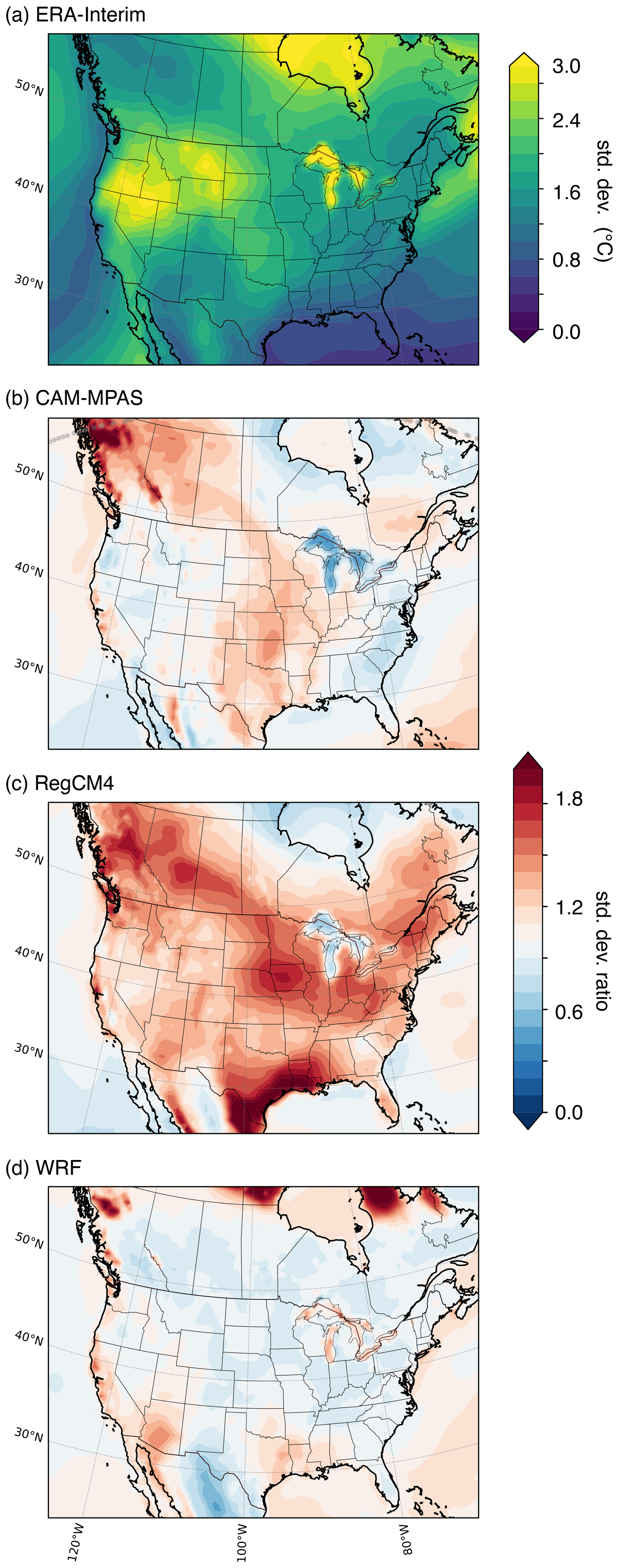
Figure 4 JJA monthly standard deviations of tas in ERA-Interim (a) and the ratio of the standard deviations  ${\mathit{\sigma }}_{\mathrm{model}}/{\mathit{\sigma }}_{\mathrm{ERAI}}$) in (b) CAM-MPAS, (c) RegCM4, and (d) WRF.

Figure 4 compares simulated standard deviations (σ_model) of monthly mean tas of each grid box to those in ERA-Interim (σ_ERAI) as the ratio ($R_{\mathit{\sigma }}={\mathit{\sigma }}_{\mathrm{model}}/{\mathit{\sigma }}_{\mathrm{ERAI}}$). ERA-Interim shows the strongest variability in the PNW region in the United States (Fig. 4a). CAM-MPAS is able to capture this variability center as indicated by R_σ being close to one over the region (Fig. 4b). However, it overestimates the tas variability in western Canada and the central US. RegCM4 overestimates the variability over most of North America, particularly over western Canada, and northern and southern central US, and the east coast (Fig. 4c). The contrast in RegCM4 skills between the mean and variability indicates that LB forcing can constrain the time mean but not necessarily the temporal variability of tas. The WRF simulation again shows very good agreement with ERA-Interim (Fig. 4d).

3.2 JJA climatology of large-scale circulations

Acknowledging that not only the upper-level dynamics but also the local land–atmosphere interactions (Bukovsky et al., 2017; Ma et al., 2018) and the upscale growth of convective systems (Qin et al., 2023) play crucial roles in tas bias, we focus on the role of the subseasonal to seasonal scale upper-level circulations through the lens of Rossby wave dynamics. This section reviews some key aspects of the JJA climatology of the upper-level circulations relevant to quasi-stationary Rossby waves. The evaluation of the model-simulated upper-level circulations over North America follows it.

As in other seasons, the JJA-mean zonal winds are characterized by the extratropical and subtropical jets but with lower wind speeds and less zonally uniform structure (Fig. 5a). The extratropical jet is nearly circum-global except for the discontinuities over the eastern Pacific and Atlantic oceans, where the subtropical jet extends from ≈20° N latitude to merge with the mid-latitude jet. Since jet streams serve as wave guides (Manola et al., 2013; Branstator and Teng, 2017; Wirth, 2020; White and Mareshet Admasu, 2025), we expect that Rossby waves propagate from the Pacific Ocean to North America along the mid-latitude as well as the subtropical jets. When Rossby waves enter the East Pacific and the West Coast of North America, they encounter complex mean wind patterns, where the traditional assumptions for the base state in Rossby wave dynamics – namely, zonally uniform flow with zero meridional winds – are not valid. Indeed, over the Western US, the mean zonal and meridional wind speeds are comparable; the former range from 12 to 20 m s⁻¹, while the latter can be as high as 8 m s⁻¹ (Fig. 5b). Therefore, the role of the meridional wind in Rossby wave dynamics should not be ignored in this region.

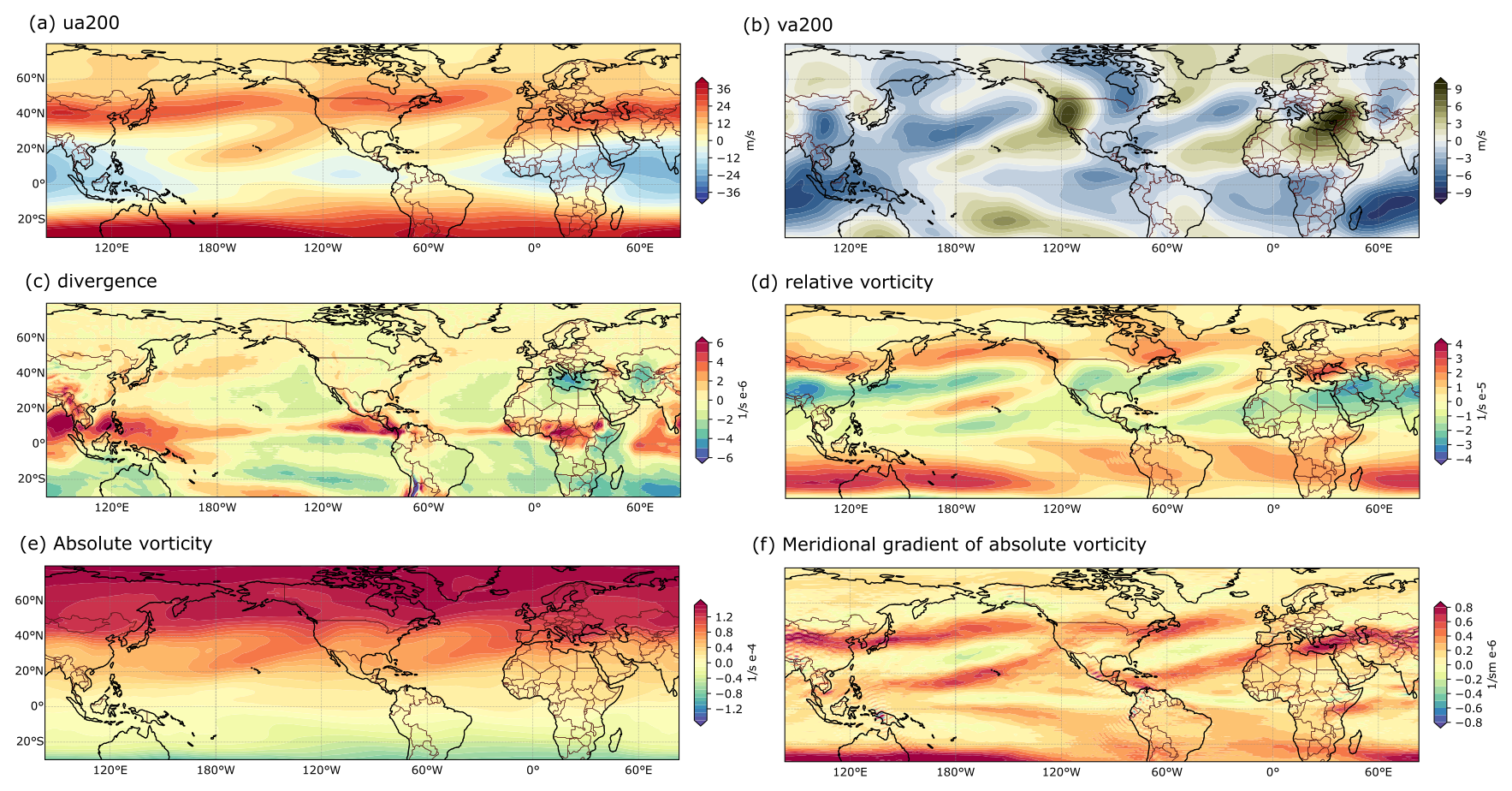
Figure 5 The 30-year JJA-mean winds at the 200 hPa level in the ERA-Interim data: (a) zonal wind, (b) meridional wind, (c) divergence, (d) relative vorticity, (e) absolute vorticity, and (f) meridional gradient of absolute vorticity.

Vorticity and divergence are essential for Rossby wave dynamics and are also shown in the figure (Fig. 5c and d). One aspect of the jet's waveguide nature stems from the strong horizontal shear at its edges, which enhances the vorticity gradient. Also, the interaction between vorticity and divergence alters the local vorticity balance (via vortex stretching, $-\mathit{\eta }(\mathrm{\nabla }\cdot \mathbf{v})$), acting as a source of relative vorticity anomalies, often called Rossby Wave Sources (RWS) (Sardeshmukh and Hoskins, 1988). In JJA, local maxima and minima of the mean relative vorticity near the jet create the meridionally banded structure over the Pacific and Atlantic oceans. The relative vorticity maxima near the subtropical jets are also strong enough to produce zonal anomalies of the absolute vorticity (Fig. 5e). As a result, two sharp meridional gradients of absolute vorticity, or the regions of strong restoring force for Rossby waves, exist upstream of North America from the northern and tropical Pacific (Fig. 5f). In the tropics, strong 200 hPa divergence is co-located with regions of intense deep convective precipitation, most notably in the Asian Monsoon. This massive latent heating drives a downstream dynamical response, maintaining a region of pronounced upper-level convergence over the Mediterranean and the Middle East (Rodwell and Hoskins, 1996). Further north, a secondary divergence anomaly is observed along the southern flank of the North Pacific jet, associated with the midlatitude storm track. Those are potential source regions for Rossby waves propagating to North America.

For evaluating the upper-level circulations in the downscaling simulations, we focus on three variables: the mean 200 hPa zonal winds (ua200), meridional winds (va200), and zonal anomalies of geopotential heights (zg200) (Fig. 6). As explained in Sect. 2.2, the modeled fields from the two LAMs are patched with the same fields of ERA-Interim outside the model domain, a visualization also used by Denis et al. (2002b). We use the full fields here instead of the differences between the simulations and ERA-Interim to emphasize the overall spatial patterns and unphysical discontinuities (difference plots are provided in Fig. B1). Ideally, for LAMs, the mean circulation across the LBs appears seamless. This is the case with the WRF simulation (Fig. 6d, h and l), where its spatial patterns are identical to those from the ERA-Interim even inside the model domain; the contour plot for the difference from ERA-Interim confirms negligible bias (Fig. B1). The geopotential height is slightly and uniformly higher within the WRF domain than ERA-Interim, but identifying the sources of zg200 bias in WRF is left for future work.

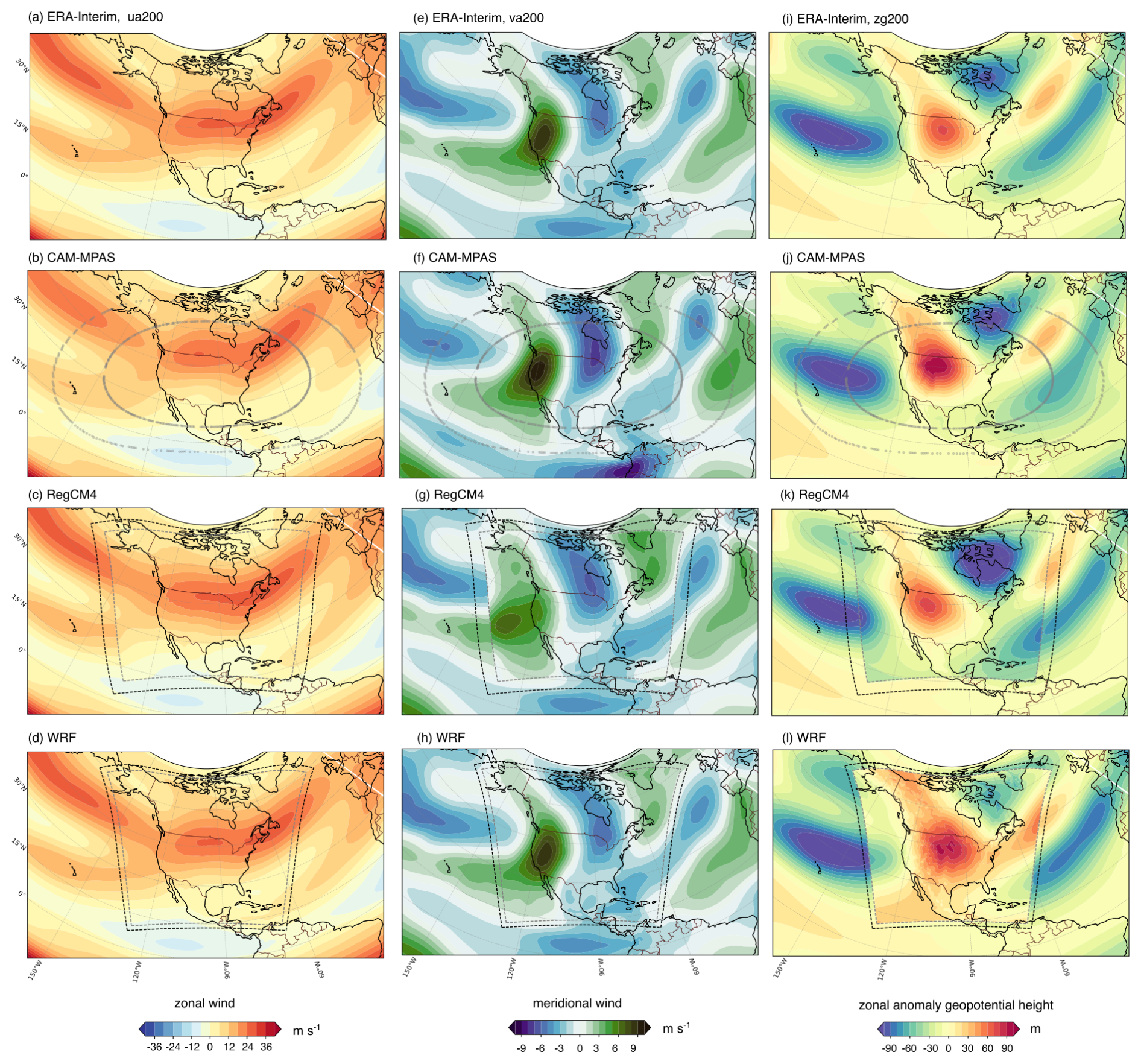
Figure 6 The JJA-mean zonal winds (a–d), meridional winds (e–h), and zonal anomaly geopotential height (i–l) at the 200 hPa level over the NA-CORDEX domain, in ERA-Interim (a, e, i), CAM-MPAS (b, f, j), RegCM4 (c, g, k), and WRF (d, h, l). In the second row for CAM-MPAS, the gray markers denote the approximate boundaries between the high-resolution domain, transition zone, and low-resolution domain of the variable-resolution grid. In the bottom two rows for RegCM4 and WRF, the black dashed lines denote the original model domain boundary, and the gray dashed lines denote the boundaries of the post-processed NA-CORDEX data, which excludes the blending zone near the lateral boundaries (24 and 10 grid points for RegCM4 and WRF, respectively; see also Table 1 and Appendix B1). For RegCM4 and WRF, the regional model data are shown within the NA-CORDEX data domain, and ERA-Interim data are used outside the domain, including the blending zone.

The overall patterns simulated by RegCM4 look reasonable, but discontinuities are apparent along the boundaries (Fig. 6c, g and k). Inside the model domain, the subtropical jet entering California is weaker than ERA-Interim, and the va200 and zg200 patterns are shifted to the west. These patterns are time-invariant stationary waves that exist in the mean circulation, which we distinguish from quasi-stationary waves defined as the perturbation on the mean. CAM-MPAS captures the general structure of the upper-level circulations without artificial boundary effects (Fig. 6b, f and j); however, the jet core is weaker and located more northwestward than ERA-Interim, while the meridional wind speeds are overestimated (also see Fig. B1a and d). Consistent with the overestimated va200 speeds, the zg200 zonal anomaly over North America is too high compared to ERA-Interim (Fig. 6i and j). In other words, the amplitude of the time-mean stationary waves is too strong. The position of the positive maxima of zg200 anomaly coincides with the spatial structure of the mean warm bias in tas (Fig. 3b), indicating the contribution of the upper-level mean wind bias to the tas mean bias. On the other hand, in the case of RegCM4, the mean bias in the upper-level winds and warm bias in tas do not spatially overlap.

3.3 Model biases in Rossby wave propagations

The mean wind biases shown above imply that the waveguide structure for Rossby waves is also biased in the model simulations. Before evaluating the model-simulated Rossby wave propagations, we first diagnose major waveguides in the ERA-Interim data. A commonly used diagnostic is the stationary wavenumber, K_s (Hoskins and Karoly, 1981), which is derived from the dispersion relationship of Rossby waves under a zonally uniform state with zero meridional winds. The stationary wavenumber is defined as

$$\begin{array}{}\text{(4)}& K_{\mathrm{s}}^{\mathrm{2}}={\displaystyle \frac{{\stackrel{\mathrm{‾}}{\mathit{\eta }}}_y}{{\stackrel{\mathrm{‾}}{u}}_{\mathrm{M}}}}.\end{array}$$

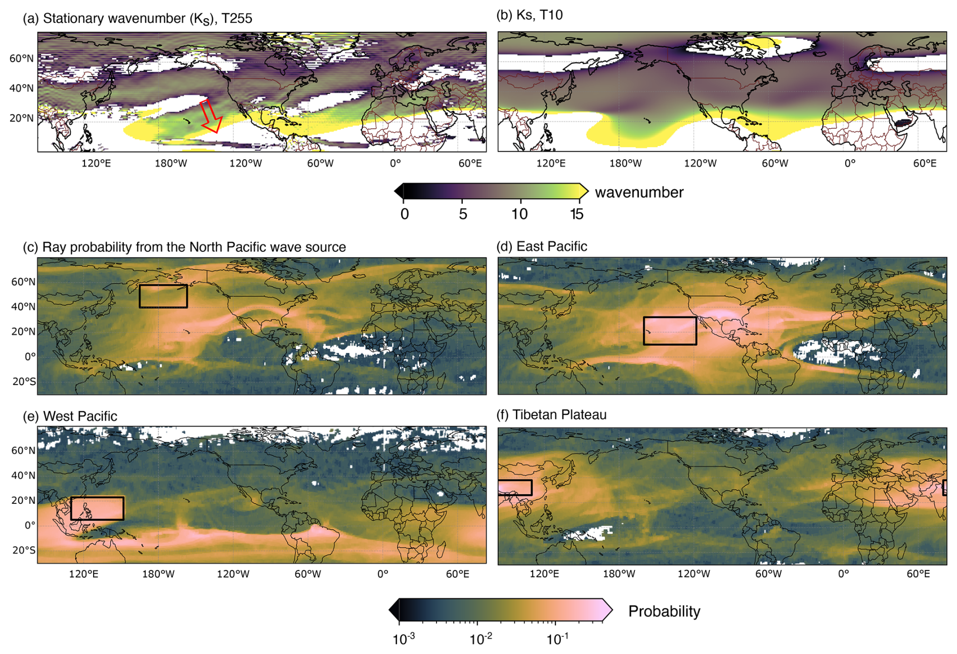
Figure 7 Waveguides for (quasi-)stationary Rossby waves, (a, b) diagnosed by stationary wavenumber, K_s, (Eq. 4) and (c–f) by the probability of Rossby wave propagation obtained by the LZ15 ray tracing method. In (a), K_s is calculated from the JJA climatology from ERA-Interim on its native grid resolution (T255), while in (b) it is calculated from the smoothed climatology (T10), same as the background state for the ray tracing. The grid boxes with imaginary K_s are shown in white. The ray tracing results are presented separately for each source region: (c) northern North Pacific, (d) eastern subtropical Pacific, (e) western tropical Pacific, and (f) Tibetan Plateau. Probability is calculated for each grid box as the fraction of rays reaching the grid box over the total number of rays traced from a source region.

It indicates where Rossby waves can propagate and where they are likely to be trapped or reflected; regions with real-valued K_s are conducive to Rossby wave propagation, while those with imaginary K_s are not. Over the regions where K_s is real-valued, it acts as a cut-off filter for stationary waves. When K_s is small (e.g., in strong westerlies), the total wavenumber allowed is low, so only very long waves can exist as stationary waves. Stationary wavenumber also acts like the refractive index for the optical wave solution, such that Rossby wave rays (paths of group velocity vectors) bend toward regions of higher K_s (see Hoskins and Ambrizzi, 1993; Li et al., 2018, and Appendix C).

In Fig. 7a, we apply this metric to the JJA climatology of ERA-Interim at each grid point, assuming that the metric K_s is locally applicable (e.g., Hoskins and Ambrizzi, 1993; Henderson et al., 2017; Hoskins and Woollings, 2015). The grid boxes with imaginary values are shown in white in the figure. It depicts the two waveguides along the mid-latitude and subtropical jets into North America, consistent with the mean wind patterns. Interpretation of K_s as the refractive index suggests that a Rossby wave excited within the local maximum of K_s, associated with the mid-latitude jet, is trapped within the jet and propagates zonally since the strong vorticity gradients to the north and south refract back the wave. On the other hand, a Rossby wave excited in the subtropical jet would be refracted southward toward the equator with higher K_s (the red arrow in the figure) toward the critical latitude where waves cannot propagate further, rather than traveling into North America. South of the mid-latitude jet over the central Pacific, there is another prohibited region where the zonal winds are near zero, and the meridional gradient of absolute vorticity is slightly negative (see Fig. 5). Figure 7b shows the same diagnostic but calculated from the smoothed background state, which is more appropriate for the WKB approximation underlying the dispersion relationship (Appendix C). The overall waveguide structure is similar to that in Fig. 7a, but regional maxima (i.e., waveguides) are blurred, and the prohibited region over the central Pacific is replaced by small real values.

The assumptions of zonally uniform flow and zero meridional winds are not valid over the eastern Pacific and western North America, prompting us to perform ray tracing by LZ2015 to confirm the waveguide structure. To do this, we need to specify the locations of the wave sources. Previous studies suggest several remote sources of Rossby waves reaching North America during the summer, including the East Asian and Indian Monsoon regions, the western Pacific, the Tibetan Plateau, and the Mediterranean (e.g., Ting, 1994; Ambrizzi et al., 1995; Trenberth et al., 1998; Wang et al., 2001; Lau and Weng, 2002; Ding and Wang, 2005; Wang et al., 2007; Lin, 2009; Li et al., 2015, 2019). Most of them found Rossby waves propagating along the mid-latitude jet, but several studies suggested Rossby wave propagation along the subtropical jet from the central and eastern tropical/subtropical Pacific to North America (Li et al., 2019; Chang et al., 2023a; Chen et al., 2023; Lubis et al., 2024). Those waves can be initiated during the Madden–Julian Oscillation phases 5 and 6, travel across North America, and break over the Atlantic Ocean (Chang et al., 2023a). A closely related subseasonal variability, the boreal summer intraseasonal oscillation, is also found to enhance convective heating during particular phases, which triggers Rossby wave trains that tend to place a high-pressure ridge over the Pacific Northwest region (Lubis et al., 2024).

Ensemble ray tracing is performed as described in Sect. 2.3.1 for the source locations suggested by previous studies and by our preparatory analyses (Appendix C2). Results from four source locations are shown in Fig. 7 using the ERA-Interim climatological winds as the base state. Rossby waves excited in the northern North Pacific (NP) (Fig. 7c) and eastern tropical/subtropical Pacific (EP) (Fig. 7d) have significantly higher probabilities of propagating over North America than those originating from other areas. Waveguides extending from the eastern subtropical Pacific (20–30° N) to North America are evident for the waves originating from both the NP and EP regions.

Most waves excited in the West Pacific region travel southeast across the equator owing to the tropical easterly zonal wind and the monsoonal northerly meridional winds (Li et al., 2019). The Tibetan Plateau generates Rossby waves that propagate westward; some of these waves arrive in North America from the east, while others turn eastward over North Africa and propagate along the jet stream. Some of those results may appear inconsistent with previous studies, and it is possible that wave activities originated from the other locations to reach North America, particularly in other seasons (Wang et al., 2020; Zhang et al., 2024), through non-linear processes such as Rossby wave breaking and associated wave reflection (Abatzoglou and Magnusdottir, 2006), or by the interactions of propagating Rossby waves and the background divergent circulation (Sardeshmukh and Hoskins, 1988; Li, 2020), which are not included in the linear ray theory. Nonetheless, one-point correlation maps for meridional winds are consistent with the ray tracing result, such that statistically significant lead/lag correlations over North America are found only when the base points are specified in the NP and EP regions. Given those results, we consider it reasonable to focus on the upwind source regions of NP and EP to evaluate regional downscaling simulations.

Sub-samples of individual ray trajectories from these two regions are shown in Fig. 8 to illustrate actual wave rays and their relationship to the initial zonal wavenumber (k₀) and background circulations. The figure uses climatological July winds as the base state, but the result is qualitatively similar to those obtained with June or August climatological flows (not shown). Rossby waves excited over the NP region with smaller k₀ (i.e., longer wavelengths) tend to travel south/southeast toward the subtropical eastern Pacific, then turn east/northeast to reach North America. The climatological flow patterns immediately south of the NP source region have the northerly meridional winds of $\approx -\mathrm{5}$ m s⁻¹ with comparable or even weaker zonal winds (Fig. 5a and b). Also, the meridional group velocity is inversely proportional to the second power of the wavenumber; thus, smaller wavenumbers favor larger group velocity (Eq. C12). Those two aspects likely facilitate southward propagation from NP. On the other hand, those initiated with larger k₀ tend to propagate along the mid-latitude jet and travel across North America near the US–Canada border (Fig. 8c).

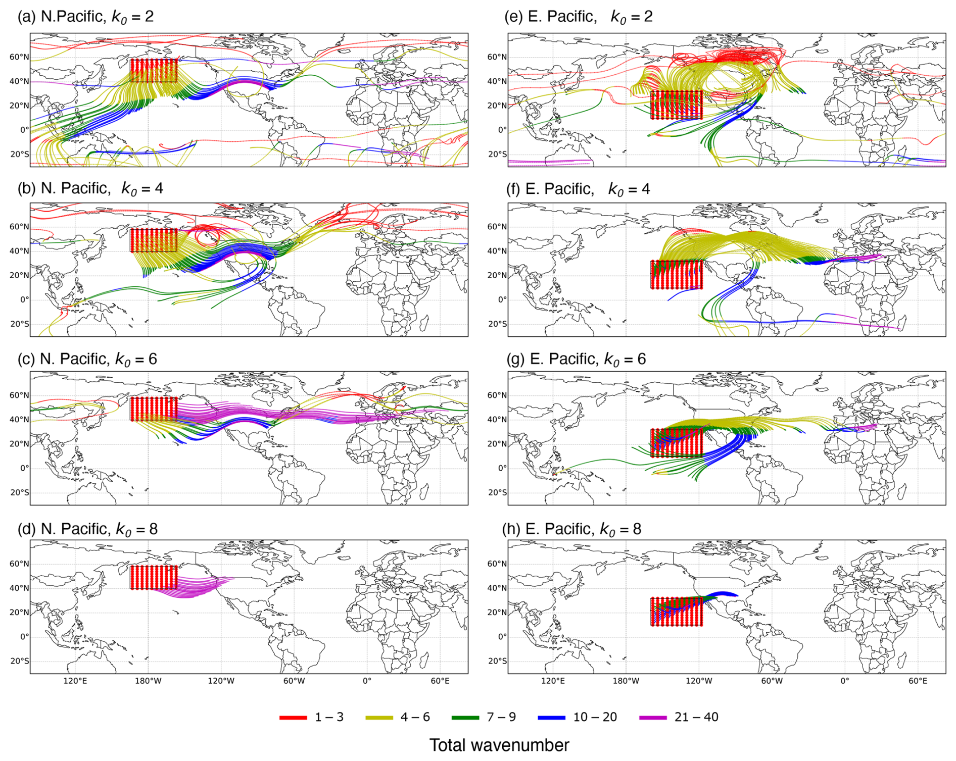
Figure 8 Samples of Rossby wave rays using the climatological July circulation from ERA-Interim as the base state. Rays initiated from the North Pacific source region are shown on the left column, starting with different initial zonal wavenumbers: (a) k₀=2, (b) k₀=4, (c) k₀=6, and (d) k₀=8. The right column shows the rays from the tropical East Pacific source region with: (e) k₀=2, (f) k₀=4, (g) k₀=6, and (h) k₀=8. Line colors represent time-dependent total wavenumber K (Eq. C11), and red dots show the source point location. Rays are terminated when the total wavenumber reaches 40 (wavelength of ≈1000 km), assuming that they are not small-amplitude perturbations at the geostrophic scale anymore (wave-breaking).

Located more southeastward, the EP region is situated within the northward meridional background winds (Fig. 5b). Consistently, the waves excited here with smaller k₀ first propagate north, and turn around at the northern edge of the mid-latitude jet (Fig. 8e and f). The initial northward propagation is not obvious in the K_s diagnostics. Similar to the waves from the NP region, waves initiated with larger k₀ tend to be trapped within the mid-latitude jet and propagate more zonally. For both source regions, waves with even larger   k₀ are not able to propagate across North America (Fig. 8c, d, g and h) (Li et al., 2019). The result illustrates the sensitivity of Rossby ray propagation to the base state, highlighting the profound impact of mean-circulation bias on modeled Rossby wave propagation.

The stationary wavenumber K_s and LZ15 ray tracing agree on the waveguide formed by the mid-latitude jet, which is more effective for waves initiated with k₀≈6 in the LZ15 framework. For waves with smaller k₀, LZ15 results diverge from the waveguide depicted by K_s on: (1) southward propagations over the central Pacific, where K_s prohibits wave propagation, (2) northeastward waveguides by the subtropical jet, where K_s implies equatoward propagation toward the critical latitude south of the jet, and (3) northward propagations off the West Coast guided by southerly meridional winds. As shown below, wave activity flux patterns from TN01 are consistent with the LZ15 result, and meridional winds off the West Coast play an important role in understanding model biases in Rossby wave propagation and their downwind impact over North America. More sophisticated constructions of the background state for K_s have been suggested (e.g., White and Mareshet Admasu, 2025), which may produce a waveguide structure that is more consistent with the LZ15 and TN01 diagnostics.

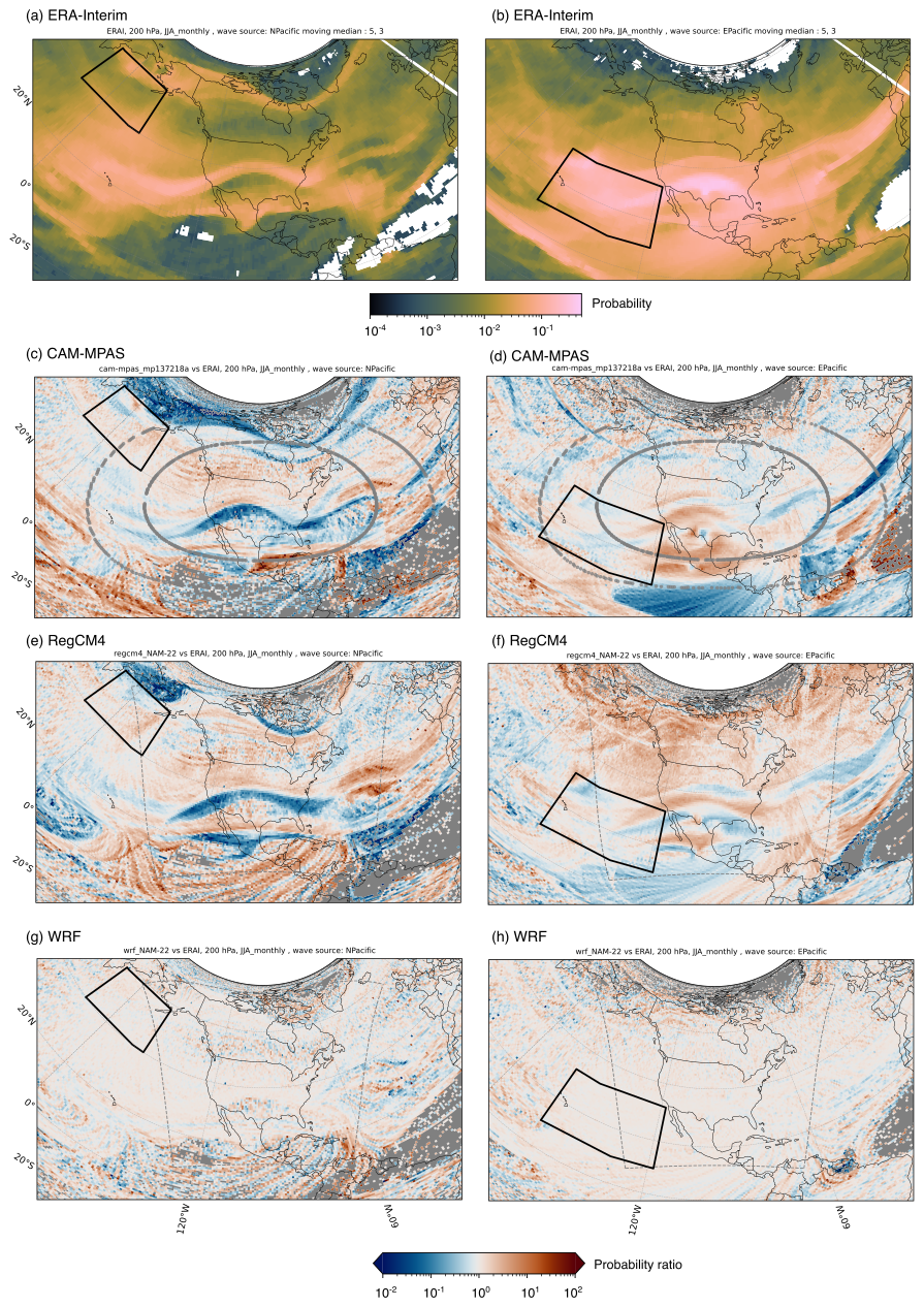
Figure 9 Probability of Rossby wave propagation from the North Pacific and East Pacific source regions obtained from ERA-Interim (a, b), and the ratio of the probabilities as $R=P_{\mathrm{model}}/P_{\mathrm{ERAI}}$ for CAM-MPAS (c, d), RegCM4 (e, f) and WRF (g, h). $R=\mathrm{1}={\mathrm{10}}^{\mathrm{0}}$ means the equal probabilities of ray propagation in the model and ERA-Interim. A five-point running average is applied before plotting to reduce noise, primarily over the regions of low probabilities.

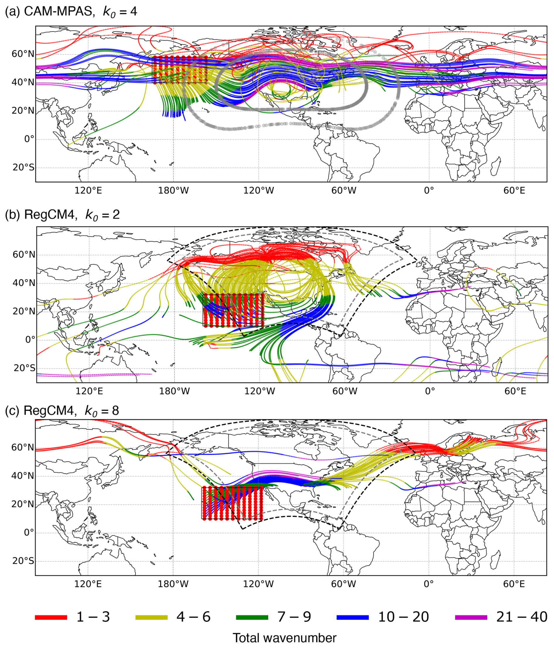
Figure 10 Samples of Rossby wave rays using the climatological July circulation from the downscaling models as the base states. (a) CAM-MPAS for waves initiated in the North Pacific source region with initial zonal wavenumber k₀=4, (b) RegCM4 for waves from the East Pacific source region but with k₀=2, and (c) RegCM4 with k₀=8. Line colors represent time-dependent total wavenumber K (Eq. C11), and red dots show the source point location. Rays are terminated when the total wavenumber reaches 40 (wavelength of ≈1000 km), assuming that they are not small-amplitude perturbations at the geostrophic scale anymore (wave-breaking).

We evaluate the downscaling models by comparing the ray propagation probabilities obtained with the LZ15 framework, using the ratio of model to reanalysis probabilities, $R_{\mathrm{p}}=p_{\mathrm{model}}/p_{\mathrm{ERAI}}$. The ray probabilities in the WRF simulation are almost identical to those in the ERA-Interim (R_p≈1 in Fig. 9g and h), as expected from the small bias in the upper-level circulations. For the other two models, biases in jet and meridional wind speeds lead to significantly different wave-propagation patterns from those in ERA-Interim. For the waves initiated in the NP region, CAM-MPAS overestimates the probabilities over Canada and northern CONUS, and underestimates them over the southern part of CONUS (Fig. 9c). This is likely the result of the northward-shifted mid-latitude jet and overestimated southerly winds over the West Coast (Fig. B1a and d), which promote more zonal propagations at higher latitudes instead of traveling to the south. Such propagations are seen for the waves initiated with relatively small zonal wavenumbers (Fig. 10a for k₀=4). For those waves, the mean circulation patterns in CAM-MPAS support longer-lived, circumglobal propagation that passes over North America twice, thereby increasing propagation probabilities. Such long-lived waves are rare for the same initial zonal wavenumbers with the ERA-Interim base state. For the waves from the EP region, stronger southerly winds over the West Coast region likely allow more waves to travel north, but the slightly weaker and wider jet in CAM-MPAS appears to be a less effective waveguide, spreading the rays more widely over North America, particularly to the south of the jet where CAM-MPAS simulates higher propagation probabilities (Fig. 9d).

The Rossby wave probabilities in RegCM4 (Fig. 9e and f) show some similarity with those in CAM-MPAS, likely due to the two models sharing the mean circulation biases over the western part of the NA-CORDEX domain (Fig. B1d and e). We can see more dense lines of wave rays emanating north from the EP source region (west of 120° W) in the RegCM4 ray tracing than in ERA-Interim (Fig. 10b vs. Fig. 8e), where stronger southerly winds are noted in the RegCM4 simulation (Fig. B1e). At the same time, the overestimated southerly winds appear to limit the southward wave propagation from the NP region, thus shifting the probabilities northward over North America (Fig. 9e). The mean wind patterns over North America in RegCM4 allow waves from the EP region with larger k₀ to travel farther than in the ERA-Interim base state, for example, for the initial zonal wavenumber of eight (Fig. 10c vs. Fig. 8h). Those waves also contribute to the higher probabilities from the EP region. LB effects are not apparent in the RegCM4 ray-tracing results. This is due to the smoothing of the base state after the RegCM4 and ERA-Interim data are patched onto the global grid, thereby effectively weakening discontinuities at the lateral boundaries.

Overall, biases in the large-scale circulations in CAM-MPAS and RegCM4 tend to increase wave-propagation probabilities in the northern part of North America, particularly in the RegCM4 base state. Additionally, the probabilities for Rossby waves around 40° N over CONUS from the NP region are underestimated, whereas the waves from the EP region are overestimated by both models. Those two biases would not simply cancel each other out, because Rossby waves propagating from the NP region tend to have higher wavenumbers (shorter wavelengths) over North America than those from the EP region (Fig. 8). The smaller waves from the NP region may be more susceptible to breaking. In contrast, those from the EP region in wavenumbers four to six may have higher probabilities of resonating with Rossby waves of similar wavelengths but different frequencies (Petoukhov et al., 2013; Coumou et al., 2014). Those non-linear processes are not part of our diagnostics, though.

The shifted Rossby wave propagations in CAM-MPAS and RegCM4 may disrupt the spatiotemporal correlations between Rossby waves and surface climate, as seen in the 2009 heatwave example in the Introduction. In the two model simulations, the biases in Rossby wave probabilities and tas variability are both large over the Pacific Northwest, suggesting a connection between them. We explore the connection in the following sections.

3.4 Wave activity flux and surface air temperature

We begin with a global view of wave activity in ERA-Interim. The area with the most vigorous quasi-stationary Rossby WA in the JJA season is the Pacific Ocean, followed by the Atlantic Ocean, both characterized by large flux and strong divergence of the W-vector (Fig. 11a). We interpret the areas of divergence as indicating WA sources. Vigorous WA fluxes from the NP and EP wave sources converge on the West Coast of North America, then propagate across the continent to diverge out from the East Coast, in general agreement with the 2009 heatwave case (Introduction). The pathways from the two source regions agree with the ray-theory result, including the initial southward propagation from the NP region and waveguiding by the subtropical jet.

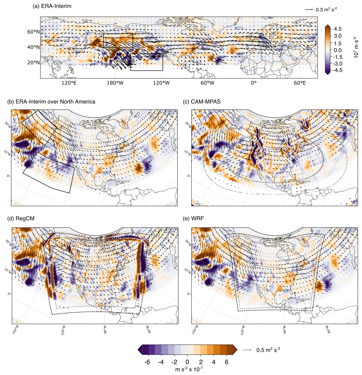
Figure 11 JJA climatology of horizontal components of the W-vector (arrows) and its divergence (color) at the 200 hPa level in (a, b) ERA-Interim, (c) CAM-MPAS, (d) RegCM4, and (e) WRF. The regions between 10° S and 10° N are masked because the Quasi-geostrophic assumption for the W-vector is not generally valid. The black boxes in (a, b) represent the source locations used for the ray tracing in Sect. 3.3. Note that the vector scale and color limits are different between (a) and the other panels. In the RegCM4 result, a Gaussian filter is applied to the relaxation zone.

The bottom four panels in Fig. 11 compare the W-vector patterns over North America in the downscaling models and ERA-Interim. The most notable feature is the bands of strong divergence/convergence pairs along the LBs in the RegCM4 simulation (Fig. 11d), which strongly suggests inconsistency between ERA-Interim and RegCM4 circulations, even considering the removed relaxation zone (Sect. 2.2). Although some spuriously large W-vectors emanating from LBs should be ignored, those downwind over the Pacific coastal area and the Pacific Northwest region are calculated fully from the model data, thus reliable. There, the W-vector in RegCM4 is oriented more zonally than in ERA-Interim, and some of the WA flux appear to originate at the LB rather than from the NP and EP regions. Not only the coastal region, but also the WA fluxes over the central US differ between RegCM4 and ERAI; RegCM4 simulates a more northerly W-vector, while ERA-Interim suggests a more zonally propagating flux. The W-vectors in the WRF simulation are almost identical to those from ERA-Interim (Fig. 11e); subtle linear structures in the divergence pattern parallel to the lateral boundaries may be due to the removal of the relaxation zone in the W-vector calculation. The global VR simulation of the CAM-MPAS model does not suffer from such artifacts (Fig. 11c). However, the zonal propagation of the W-vector is shifted northward from the US to Canada, creating an anticyclonic rotation over the central US, possibly due to the overly strong positive geopotential anomaly (Fig. 6j). With this northward shift, the W-vector divergence over the East Coast of the US, as seen in ERA-Interim, is replaced with weak convergence in CAM-MPAS. In addition, the W-vector divergence in CAM-MPAS is overly strong near the coastlines and mountain ranges on the West Coast compared to other models and ERA-Interim. We have examined the variance spectra of surface topography, vertical velocity, and horizontal winds, but there is no indication that the topography and wind kinetic energy in CAM-MPAS differ significantly from those in other models (Fig. B3). Topography-related processes in the CAM-MPAS downscaling simulations will be investigated in future work, potentially helping to explain the strong WA flux divergence over the mountainous region.

How are the differences in the WA flux patterns reflected in the regional climate? We first look at the lead/lag correlations between the 5 d running mean zg200 anomalies across North America and the divergence of the W-vector averaged over the West Coast region, where we see strong convergence in the climatology of ERA-Interim (Fig. 11a). Each time series consists of daily data spanning 30 years (20 years for CAM-MPAS) of JJA seasons. The statistical significance is determined following Li et al. (2019) using the two-tailed Student's t-test against the null hypothesis of zero correlation, taking into consideration the autocorrelation of each time series in determining the degrees of freedom (Eq. 1 in Pyper and Peterman, 1998).

In ERA-Interim, statistically significant negative correlations appear upstream over the Gulf of Alaska and positive correlation just off the US West Coast around lag −2 (Fig. 12a), that is, zg200 anomalies off the US West Coast for a given day is positively correlated with W-vector divergence over the West Coast happening 2 d later (or the higher zg200 anomalies off the US West Coast are, the stronger WA flux divergence will be in 2 d later over the West Coast). CAM-MPAS can reproduce the correlation pattern, albeit weaker than ERA-Interim (Fig. 12b). RegCM4 misses the negative correlation over the Gulf of Alaska, extending the area with a positive correlation northwest toward the Gulf of Alaska (Fig. 12c). WRF with the spectral nudging can capture this lag-2 correlation pattern (Fig. 12d). At lag+4, statistically significant negative correlation appears over the SGP in ERA-Interim, creating a clear wave pattern (Fig. 12e). This negative correlation means that W-vector convergence (negative values) over the West Coast leads to a positive zg200 anomaly over SGP 4 d later. WRF generally captures this lag +4 correlation pattern, but without statistical significance over SGP (Fig. 12f). The other two models struggle to reproduce the lag +4 correlation (Fig. 12f and g).

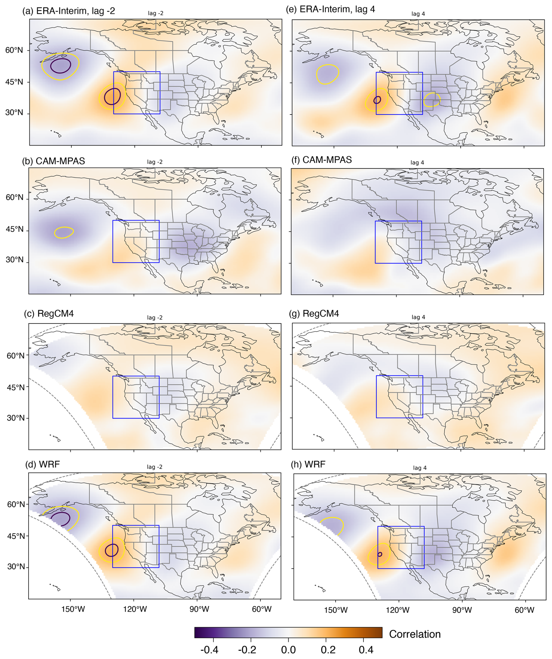
Figure 12 The lead-lag correlation between W-vector divergence averaged over the West Coast (blue box) and the 5 d running mean zg200 at each grid box. Negative lags mean that the zg200 time series leads and is shifted earlier by that amount – e.g., by 2 d in panel (a) – before the correlation is calculated against the time series of W-vector divergence. With positive lags, zg200 lags the W-vector divergence, i.e., the zg200 time series is shifted later by that amount. Yellow and black contours indicate areas with statistically significant correlations at α=0.10 and α=0.05 levels, respectively.

The tas response to the W-vector divergence closely follows the zg200 response. Again, we calculate lead/lag correlations between 5 d running mean tas anomalies at each grid point and the daily W-vector divergence averaged over the West Coast region (Fig. 13). In ERA-Interim, areas of statistically significant negative correlations appear over SGP around a lag of −2, with the maximum extent occurring when the tas anomaly is lagged by 4 d (lag +4). It suggests that the tas over the SGP tends to be higher than normal when the WA flux converges over the West Coast, particularly 4–8 d earlier. We noted that the significant lagged correlation remains when the tas anomaly is band-pass filtered for the periods between 70 and 90 d (not shown). The long timescale may indicate a role for the land surface, particularly soil moisture (e.g., Dirmeyer and Halder, 2017). The actual physical processes underlying the correlation are left for future work.

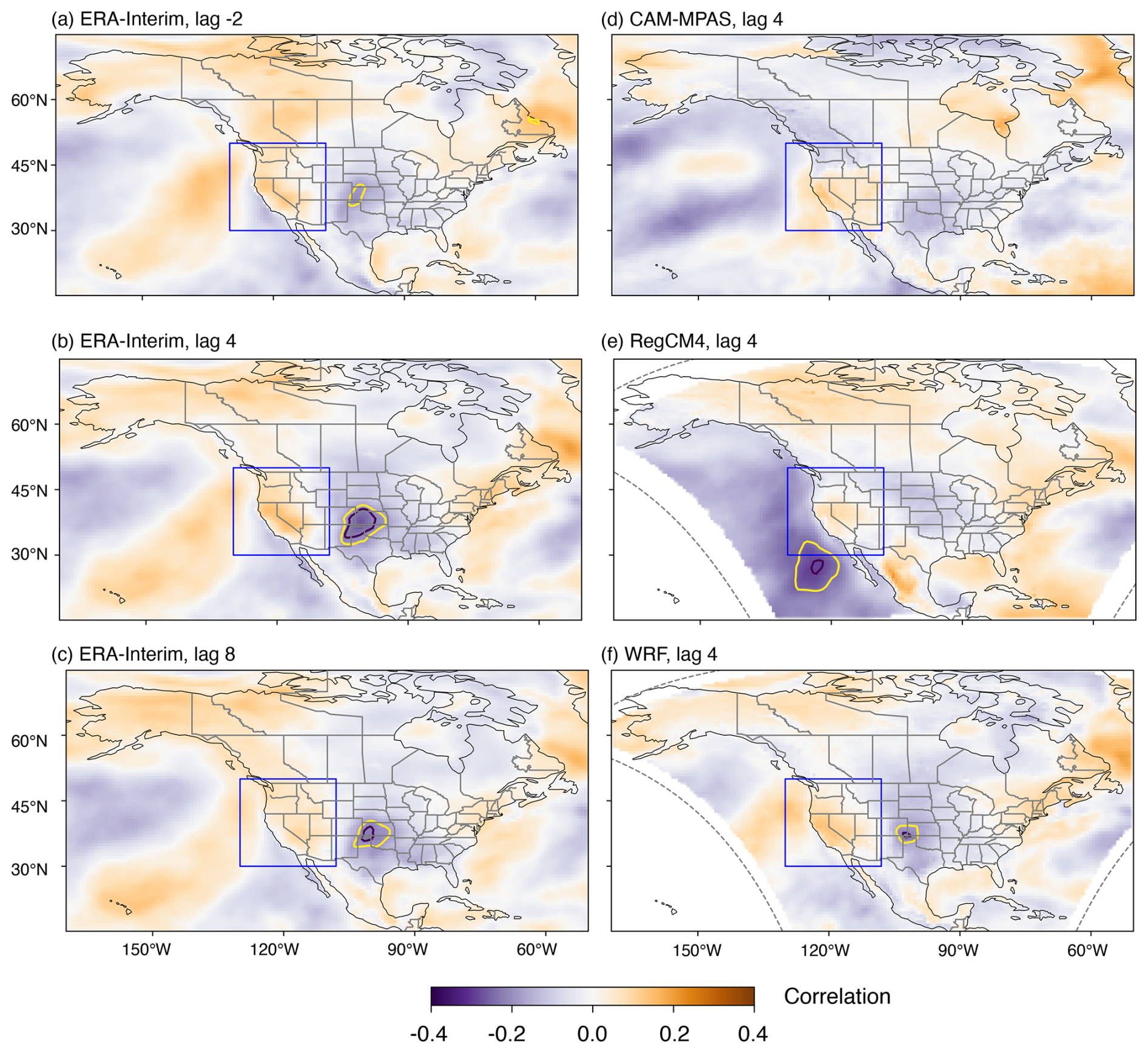
Figure 13 Same as Fig. 12, but for the lead-lag correlations between the W-vector divergence averaged over the West Coast (blue box) and the 5 d running mean (tas) anomaly at each grid box.

Focusing on the lag+4 result, WRF is the only model to simulate the significant negative correlation over SGP and the overall structure of the lead-lag correlation (Fig. 13b and f). CAM-MPAS simulates a weak negative correlation over SGP but misses the statistical significance (Fig. 13d). Also, the correlation patterns over the Pacific Northwest, western Canada, and Alaska do not agree with those in ERA-Interim. Similarly, RegCM4 misses the negative correlation center over SGP, and also simulates unrealistic negative correlation over the eastern Pacific (Fig. 13e). The inability to reproduce the W-vector–tas correlation in these two models is likely one reason for the biases of the mean and/or variability of tas over SGP (Figs. 3 and 4).

It is also possible to correlate the W-vector divergence and the errors in the simulated tas. Figure 14a presents the lead/lag correlations between the W-vector divergence averaged over the West Coast region in the RegCM4 simulation and the difference in the daily mean tas between RegCM4 and ERA-Interim at each grid point. In this case, we observe statistically significant correlations over SGP at lag +4. Those RegCM4 results suggest that accurately receiving Rossby wave signals through LBs and maintaining the large-scale circulation patterns are essential for LAMs to reproduce the cross-scale connections from Rossby waves to tas. Another example is the observation that the W-vector convergence is significantly overestimated by CAM-MPAS over British Columbia, Canada (Fig. 11). The lead/lag correlations between the W-vector divergence averaged over British Columbia, and tas errors in CAM-MPAS exhibit significant positive correlation in the same region, which also overlaps the overestimated tas variability by the same model (Fig. 4b). Part of these tas errors is attributable to out-of-sync temporal evolutions between ERA-Interim and global, free-running CAM-MPAS, which has its own internal variabilities. Nonetheless, this result illustrates another example of how model error can propagate across scales, from the biased mean wind patterns through Rossby wave forcing to tas variability.

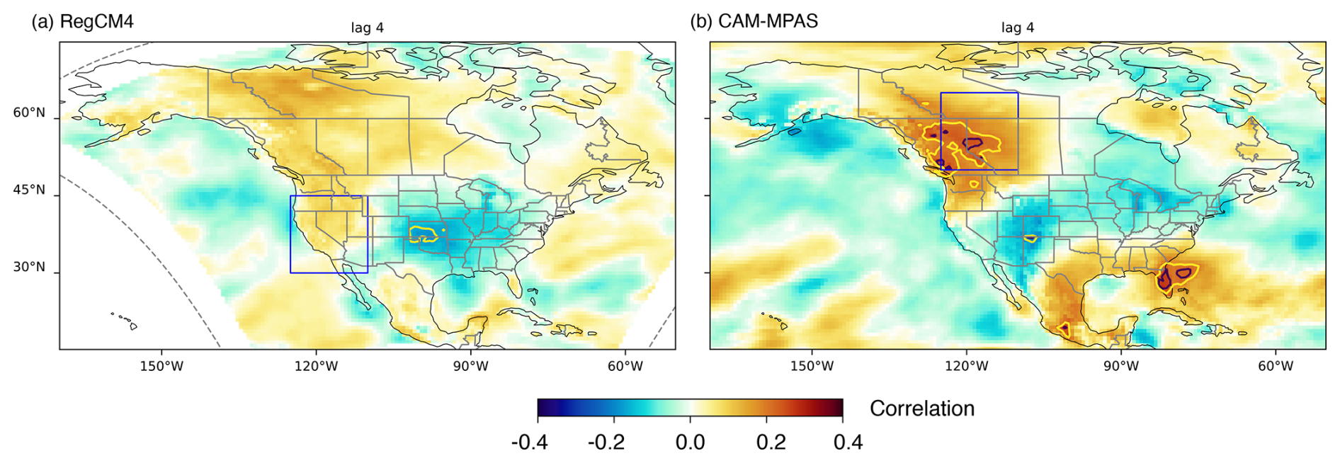
Figure 14 Similar to Fig. 13, but for the lead-lag correlations between the W-vector divergence averaged over the West Coast region in RegCM4 (a) and Canadian Pacific Northwest region in CAM-MPAS (b) and the simulation errors (model minus ERA-Interim) in the 5 d running mean (tas) at each grid box.

3.5 Rossby wave and heatwaves

In this final subsection, we demonstrate a connection between quasi-stationary Rossby wave forcing and heatwave (HW) events, and assess how the downscaling simulations replicate the connection identified in ERA-Interim. We diagnose HW events using the criteria outlined in Barriopedro et al. (2023) (their Appendix A2). Specifically, an HW event is a period of three or more consecutive days with the daily maximum tas exceeding the 95th percentile of the reference period (1981–2010, except for CAM-MPAS, for which we use 1990–2010). All seasons are included in HW identification, and the seasonal cycle is not removed; thus, this criterion favors warm-season occurrences (Barriopedro et al., 2023). Figure 15a shows the spatial distributions of the average fraction of HW days per JJA season (i.e., the number of HW days during one JJA season = 92 d). ERA-Interim indicates two local maxima, one over the southwestern US and the other over the SGP, where ≈15 % of JJA days, or about 14 HW days, are expected each summer.

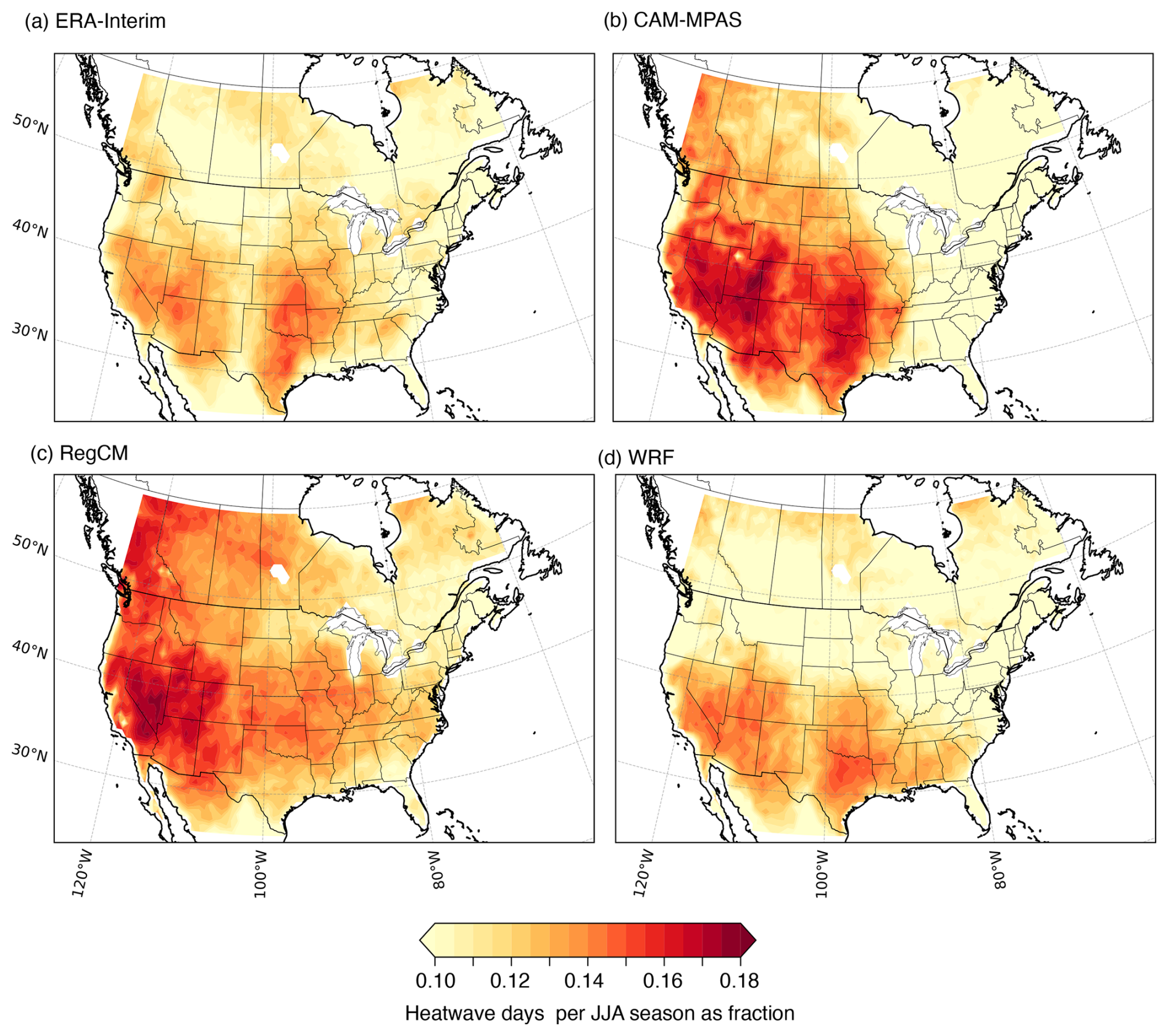
Figure 15 Fraction of the days identified as heatwaves (HWs) (or number of HW days per JJA (92) days), in (a) ERA-Interim, (b) CAM-MPAS, (c) RegCM4, and (d) WRF.

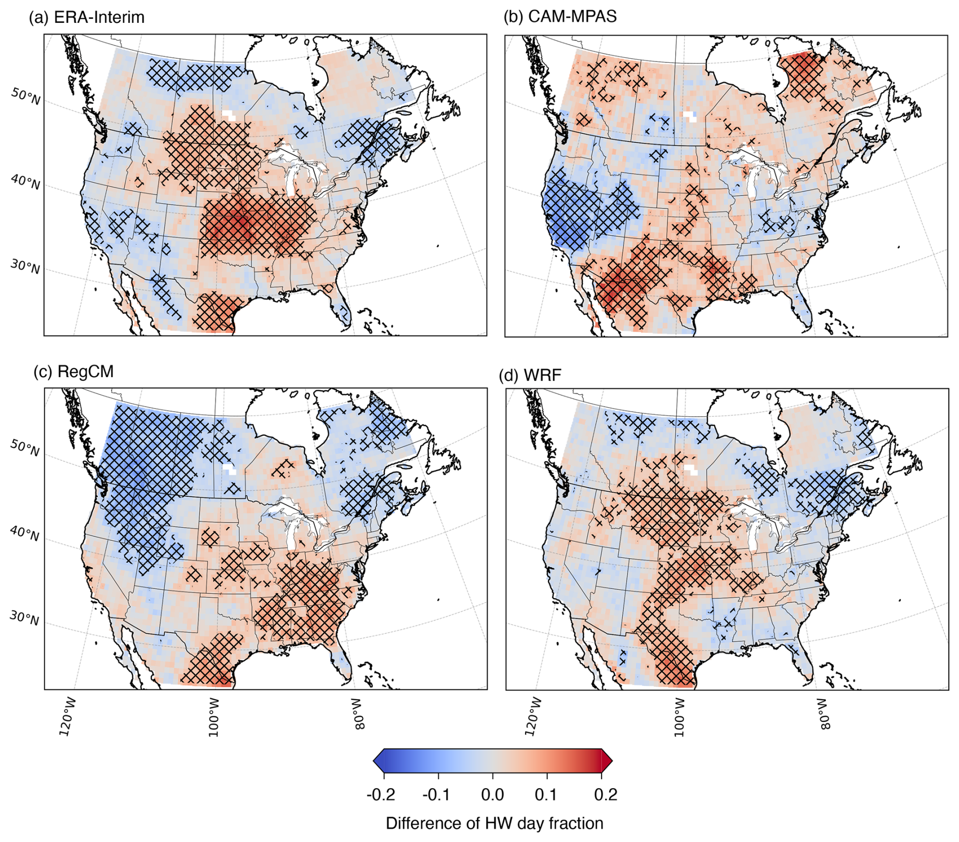
Figure 16 Difference in the fraction of the HW days, as the difference between the fraction calculated only during the extreme W-vector convergence over the Western Coast area and during the rest of the samples in (a) ERA-Interim, (b) CAM-MPAS, (c) RegCM4, and (d) WRF. The cross-hatch indicates that the difference is statistically significant at the 0.05 level.

The same HW definition is applied to the downscaling simulations, also shown in Fig. 15. CAM-MPAS can simulate the overall spatial patterns with two local maxima over the southwestern and south-central US, but overestimates the number of HW days during the summer across most of North America, except in the eastern part, where it simulates fewer HW days. RegCM4 also simulates too many HWs in the JJA season across North America, except for SGP, where it underestimates the number. The HW distributions simulated by WRF agree best with those in ERA-Interim.

How does the HW distribution change during the days with strong Rossby wave forcing? We examine the days when the WA flux convergence ($-\mathrm{\nabla }\cdot \mathit{W}$) over the West Coast region (the same region used for the lead/lag correlations) exceeds the top 90th percentile of all years. The bar graphs in Fig. B4 show how those extreme days are distributed across years. Those top 10 percentiles are not uniformly distributed but instead exhibit variability on a 3–4 year timescale, according to the ERA-Interim data. WRF reproduces this temporal distribution reasonably well, whereas RegCM4 does not. Free-running CAM-MPAS does not simulate the 2009 peak or other clusters in sync with ERA-Interim (Fig. B4b), indicating the significant roles of biased waveguide locations and/or the atmosphere's internal variability. All models agree well with ERA-Interim on the magnitude of the top 10th percentile: the average magnitude of the extreme convergence is −27, −26, −27, and −25 (10⁻⁸ m² s⁻¹) in ERA-Interim, CAM-MPAS, RegCM4, and WRF, respectively.

Calculating the fraction of HW days only on the days with extreme W-Vector convergence over the West Coast area in the ERA-Interim data, we see significantly higher HW fractions over the Midwest and the South Central US and southern Canadian Prairies, and lower fractions in the northern Canadian Prairies, Quebec, and the Southwestern US (Fig. 16a). That is, extremely rapid accumulations of WA over the West Coast region have a statistically significant impact on HW occurrences across broad regions of North America. Note that the HW fraction is roughly doubled over the Central Plains from ≈0.12–0.15 with all the samples to ≈0.2–0.3 during the extreme WA flux convergence. Examining the composite means of the HW day fractions in the downscaling simulations, the WRF simulation yields the best agreement with ERA-Interim, although it does not accurately capture the reduced HW occurrences over the southwestern US. In CAM-MPAS, the higher HW fractions are seen over British Columbia and Quebec, the Southwest, and some parts of the Great Plains. Those responses differ from what ERA-Interim describes, and are somewhat similar to the areas with overestimated variability of tas by this model (Fig. 4b). RegCM4 simulates HW surge with the extreme WA flux over the southern part of CONUS, possibly related to the more northerly WA flux over the West Coast and Great Plains in this simulation compared to the westerly WA flux in ERA-Interim (those during the extreme convergence not shown, but similar to Fig. 11). More in-depth analysis is required to conclude how the modeled HW response to WA flux is linked to the overall mean and/or variability biases of tas. Nonetheless, this diagnosis reveals a connection between extreme Rossby wave forcing and the occurrence of HWs over North America, which is accurately reproduced only by the WRF model with spectral nudging.

4 Discussions

Before summarizing our main findings, we report preliminary investigations into two outstanding questions arising from the presented results. First is the reason for the striking differences between the two LAMs, RegCM4 and WRF, in the upper-level circulations and quasi-stationary Rossby waves presented above. The two differ in many ways: numerical grid discretizations, hydrotstatic vs. non-hydrostatic dynamical core, width and weight functions of the LB buffer zones, and every component of physics parameterizations (Tables 1 and B1). Here, we focus on the impact of spectral nudging adopted in the WRF simulation for NA-CORDEX. We conducted two sensitivity simulations with WRF version 4.6.1. The only difference between the two sensitivity simulations is whether spectral nudging is used (“Nudge”) or not (“NoNudge”). The model configuration is identical to that used for the NA-CORDEX WRF simulations (Chang et al., 2015; Diez-Sierra et al., 2022b), except for using the hybrid sigma-pressure vertical coordinate that is the default option since WRF version 4.0, instead of the traditional sigma coordinate used in the NA-CORDEX simulation (Skamarock et al., 2019). It is not expected that the different vertical grid (with the same resolution) will impact the following result. Both simulations are initialized at 1 March 2010 00:00 UTC and run for nine months, ending at 30 November 2010 23:00 UTC. Only the results from the JJA months are presented. The extended periods before and after JJA are used to apply the 25–90 d band-pass filters as done in the main result to calculate the W-vector for quasi-stationary Rossby waves.

Consistent with the main result, the Nudge experiment shows little difference from ERA-Interim on the upper-level circulations, while NoNudge simulates a weaker and shifted mid-latitude jet during this particular summer (Fig. B5a and b). The NoNudge experiment produces artificial W-vector divergence/convergence pairs along the LBs, similar to the RegCM4 result, while the Nudge experiment shows no such artifacts (Fig. B5c and d). Although the simulation length is limited for a rigorous evaluation of Rossby waves, the result strongly supports the notion that spectral nudging is the dominant factor in the differences between RegCM4 and WRF. This interpretation is consistent with previous studies demonstrating the effectiveness of spectral nudging in maintaining large-scale circulations from the forcing data and their impact on the near-surface climate (Miguez-Macho et al., 2004; Alexandru et al., 2009; Castro et al., 2012).

Another question is the possibility of upscale effects on the mean winds simulated by CAM-MPAS and RegRM4 (Figs. 6 and B1). Both models simulate stronger southerly winds and weaker mid-latitude and subtropical jets off the West Coast of CONUS than in ERA-Interim, which direct Rossby waves northward to higher latitudes (Figs. 9 and 11). Since the two models have finer spatial resolutions than ERA-Interim and their dynamics are not constrained by nudging, momentum and vorticity sources that are not well resolved by ERA-Interim may be better represented by the two models. The impact of the Rockies and organized convection on Rossby waves over North America has been noted by previous studies (Ting, 1994; Stensrud, 2013; Rodwell et al., 2013).

The impact of different spatial resolutions is assessed by comparing the more recent reanalysis product, ERA5 (Hersbach et al., 2020), with ERA-Interim, as ERA5 has a grid spacing similar to that of the models examined (≈25 km). We find that the resolution differences make negligible contributions to the JJA-mean ua200 and zg200 (Fig. B6a and b). We also look at one-season average differences in va200 and zg200 between the NoNudge WRF simulation and ERA-Interim. If higher resolution is responsible for the upper-level wind differences, the NoNudge simulation might exhibit stronger southerly winds and a weaker jet, as in CAM-MPAS and RegCM4. This is not the case based on Figs. B5a and B6c and d. The va200 difference shows weaker southerly winds off the West Coast in the WRF NoNudge experiment, which is the opposite of those by CAM-MPAS and RegCM4. The seasonal means of ua200 and zg200 in NoNudge do not exhibit the same spatial patterns as those in CAM-MPAS or RegCM4. Therefore, it is unlikely that physically oriented upscale effects are the main reasons for the mean circulation differences between ERA-Interim and the two models.

In this study, quantifying large-scale biases is a common practice; we believe the novelty lies in linking circulation biases to quasi-stationary Rossby waves and, in turn, to near-surface air temperature and heatwaves. Some of the diagnostics we use could be helpful as part of climate model diagnostics packages (e.g., Eyring et al., 2020; Zhang et al., 2022; Stan et al., 2025). One use case is to identify GCMs with good skills in simulating wave sources and waveguides toward North America (e.g., Goldenson et al., 2023). Another application is obviously the evaluation of a dynamical downscaling framework, and we expect metrics to depend on the specific regions. For North America, we recommend using ray theory to track Rossby waves from the North Pacific and the Eastern tropical/subtropical regions, which “translate” the biases in the mean circulation into the likelihood of Rossby wave propagations over North America. Another useful diagnosis is the divergence/convergence of WA flux over the West Coast. Among available WA formulations, the WA budget equation derived by TN01 does not require a time average to define the perturbation component. This means we can evaluate time series of W-vector convergence, which can then be correlated with other variables, such as tas.

Despite the insights we can gain from those diagnostics, they also have limitations that must be overcome to be included in such diagnostic packages. As stated earlier, ray tracing involves integrating ordinary differential equations over time, making this technique computationally more intensive than typical evaluation methods. W-vector diagnostics involve a more straightforward calculation, but their challenge lies in the complexity of the underlying theory rather than the numerical coding and data requirements for comprehensively analyzing three-dimensional budget terms. The LZ2015 ray theory also shares the former challenge of complexity in its underlying theory, but its publicly available repository includes documentation explaining the source code, along with example calculations and references to relevant literature (Yang, 2025; Yang and Li, 2025).

Finally, all diagnostics we applied are based on the linear framework that makes several assumptions and excludes the effect of interactions with transient eddies (Teng et al., 2019), waves with finite (larger) amplitude (Huang and Nakamura, 2017), and eventual wave-breaking (Zhang and Wang, 2018), despite the crucial roles they play in extreme events (Nakamura and Huang, 2018; Chang et al., 2023b). In Appendix C, we review the linear wave theory and other common diagnostics for Rossby waves, hoping to provide guidance for those focused on regional climate. We will continue to assess the robustness of Rossby wave diagnostics and their physical relationships with other climate variables at regional scales.

5 Summary

It is well known that not only global but also regional models exhibit warm tas bias during the summer over the central CONUS (Morcrette et al., 2018). While the role of physics parameterizations is significant on the surface warm bias, a recent study by Luo et al. (2022) found that biases in the upper-level stationary waves cause significant errors in the simulated surface temperature and precipitation. Investigating the sensitivity of WRF simulations to model resolution, convective parameterizations, and use of spectral nudging, Gao et al. (2017) found that the SGP warm biases in the model are rather insensitive to the model resolution or the convective parameterization, but they were largely alleviated using spectral nudging that constrains the model to provide realistic moisture transport to the SGP region. Our results reiterate the importance of the model's ability to accurately simulate large-scale circulations, specifically the quasi-stationary Rossby wave, for dynamical downscaling over North America. We evaluate three distinct dynamical downscaling approaches to incorporate large-scale forcing: (1) a standard regional climate simulation with a LAM, represented by the RegCM4 simulation, (2) a LAM simulation with spectral nudging to constrain the large-scale atmospheric dynamics, represented by the WRF simulation, and (3) a global VR model that simulates large-scale circulations on its global grid. The first two model data are obtained from the NA-CORDEX model archive (Mearns et al., 2017), while the CAM-MPAS data is produced by our previous work following the NA-CORDEX protocol (Sakaguchi et al., 2023). We evaluate the consistency of the large-scale circulations across the model domain boundaries by patching the LAM data and the driving data, ERA-Interim, onto a single global grid, on which the upper-level circulation and Rossby wave propagation are diagnosed.

We observe a striking contrast between RegCM4 and WRF in their consistency with the large-scale circulations of ERA-Interim. A pair of short WRF simulations with and without spectral nudging suggests that the spectral nudging applied in the NA-CORDEX WRF simulation is the primary reason for the difference between the two models. Specifically, in the RegCM4 simulation without spectral nudging, the mid-latitude and subtropical jets over the eastern North Pacific are weakened, and the time-mean geopotential patterns are shifted westward, resulting in stronger southerly meridional winds over the same region. Furthermore, discontinuities in the time-mean circulation structure are apparent along LBs. The global model CAM-MPAS also suffers from mean circulation biases over the NA-CORDEX domain, featuring a weaker and northward-shifted mid-latitude jet, a weaker subtropical jet over the eastern North Pacific, and an overly strong positive geopotential anomaly that is centered over the Pacific Northwest, which also results in stronger southerly meridional winds over the West Coast area.

A linear ray theory by LZ15 proves useful for linking those circulation biases to Rossby wave paths entering North America, owing to the relaxed assumption about the meridional winds in the mean background state. In the CAM-MPAS simulation, overestimated southerly winds and weaker zonal jets allow more Rossby waves to propagate northward from the low-latitude eastern Pacific to the Pacific Northwest, particularly to British Columbia. RegCM4 exhibits the same tendency as CAM-MPAS, overestimating the probability of Rossby wave passage over the Pacific Northwest and the eastern half of Canada. The WRF model with spectral nudging reproduces the Rossby wave propagation patterns in ERA-Interim.

Another diagnostic to complement the ray theory is the energy and momentum fluxes associated with Rossby wave packets, combined as wave activity (WA). The formulation by TN01 (W-vector) also allows a non-uniform background state and non-zero meridional winds, showing WA propagation patterns consistent with the LZ15 ray theory. ERA-Interim suggests that WA flux tends to converge over the West Coast of North America, and the temporal evolution of WA flux convergence is correlated to that of tas anomaly over SGP. CAM-MPAS and RegCM4 cannot reproduce this correlation because of a biased mean circulation, leading to different Rossby wave propagation into North America: either to higher latitudes (CAM-MPAS) or at a different angle (RegCM4). We further find a relationship between extreme Rossby wave forcing (the top 10 percentile of WA flux convergence over the West Coast region) and HW occurrences across North America. This relationship is also not well simulated by CAM-MPAS and RegCM4.

The Rossby wave diagnostics used here translate large-scale circulation biases into the propagation of Rossby waves and their influence on the surface climate. This physical connection across space and scales is disrupted by biases in the mean circulation patterns in the global VR model, or by the failure to faithfully retain large-scale forcing in the LAM dynamical downscaling. For the large spatiotemporal scales of quasi-stationary Rossby waves, spectral nudging that constrains only the larger spatial scales helps the model reproduce nearly all aspects of Rossby wave dynamics and their impact on temperature anomalies across North America. Their implications are: (1) the host GCMs and global VR models need to be able to simulate the wave sources in the eastern hemisphere (e.g., diabatic heating from organized convection) as well as the mean wind patterns over the Pacific and North America to provide correct waveguide into North America and (2) spectral nudging is beneficial for dynamical downscaling using LAMs to avoid numerical artifacts from the LB treatment on incoming Rossby waves as well as to maintain the large-scale circulation patterns on which Rossby waves propagate. Although our analysis focuses on the connection between Rossby waves and surface temperature, model biases in WA could also affect precipitation in the simulations, as seen in the common dry biases over the SGP. The latter can be further explored in the future using similar Rossby wave and WA diagnostics discussed in this study.

Appendix A: 2009 heatwave

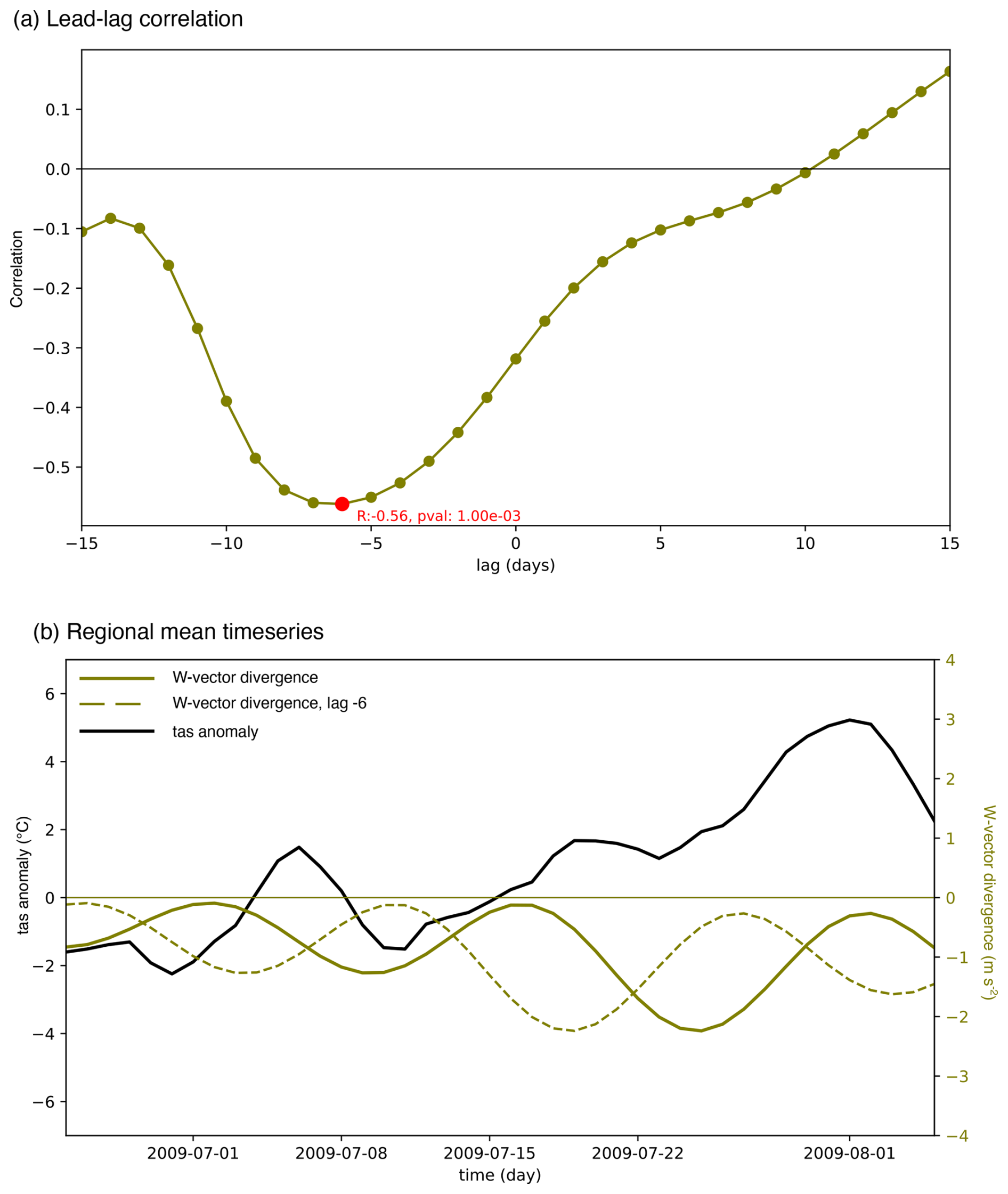
Figure A1 (a) Linear correlations between tas averaged over the Canada–US Pacific Northwest (shown by a box with black dashed line Fig. 1g and h) and the lagged divergence of WA flux averaged over the US Pacific Northwest (the red dashed-line box in Fig. 1a–c) and (b) time series of the regional-average tas anomaly (black), WA flux divergence (green), and the WA flux divergence shifted by 6 d earlier, corresponding the lag −6 at which the lag correlation reaches the absolute maximum (the lowest negative correlation).

Appendix B: Additional information for model evaluations

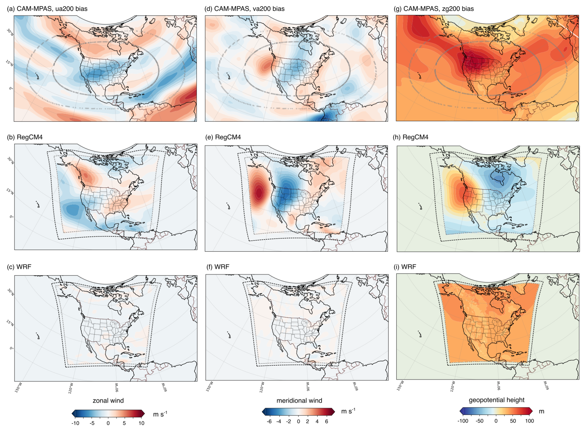
Figure B1 The JJA-mean zonal wind biases against ERA-Interim in (a) CAM-MPAS, (b) RegCM4, and (c) WRF. Corresponding meridional wind biases in (d)–(f) and geopotential biases in (g)–(i).

Table B1 Physics parameterizations used in the three downscaling models. For the references for each parameterization, readers are referred to Diez-Sierra et al. (2022b) for RegCM4 and WRF, and Sakaguchi et al. (2023) for CAM-MPAS.

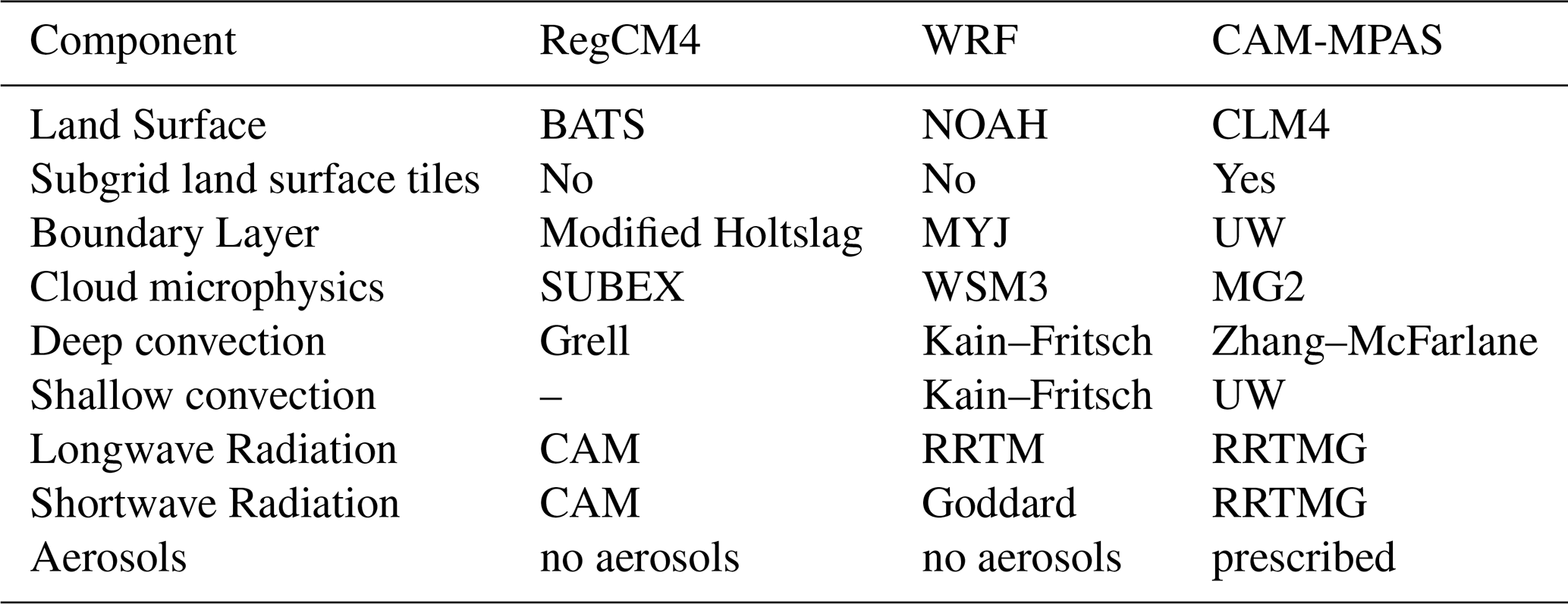
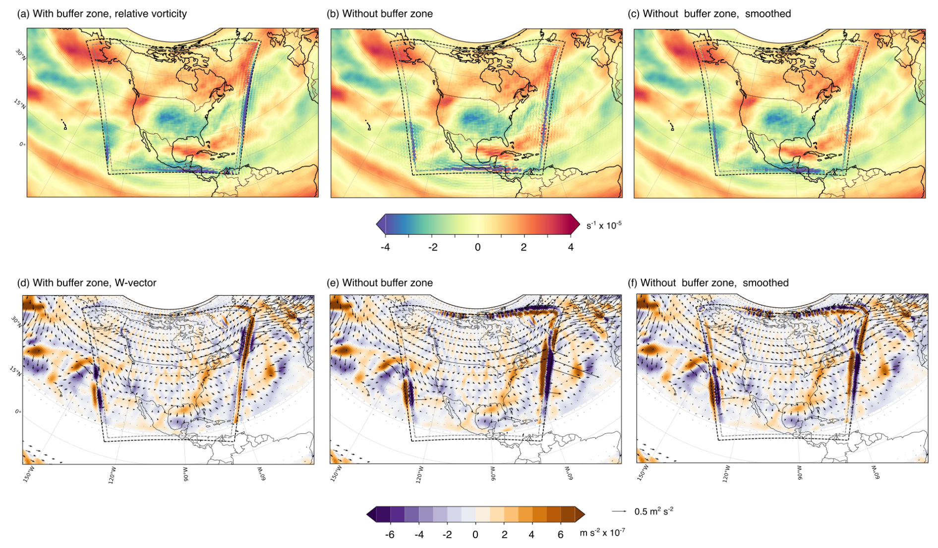
Figure B2 Illustration of the blending zone impact on derived diagnostics. The top row shows the JJA-mean vorticity calculated after remapping to the global grid and patching outside the domain with the ERA-Interim data, and bottom row shows W-vector and its divergence, using the model output with the buffer zone (a, d), without the buffer zone (b, d), and without buffer zone but Gaussian filter is applied to the (remapped) grid points located in the buffer zone (c, f).

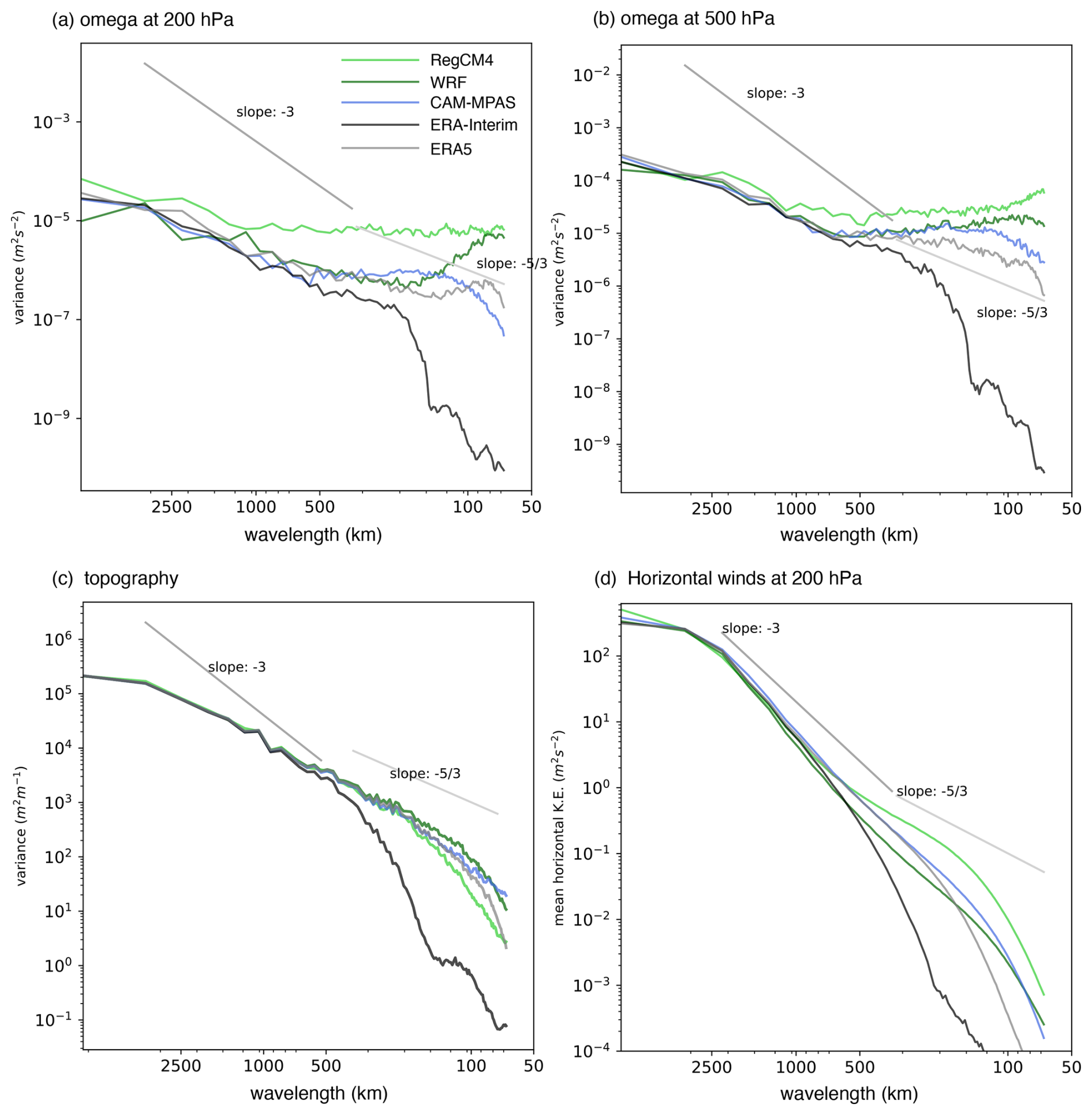
Figure B3 Power spectra of (a) pressure vertical velocity (ω, Pa s⁻¹) at the 200 hPa level, (b) ω at 500 hPa, (c) surface topography, and (d) horizontal winds at the 200 hPa level. All variables are regridded to the WRF native grid with 25 km grid spacing, then the Discrete Cosine Transform is used to calculate the spectra (Denis et al., 2002a).

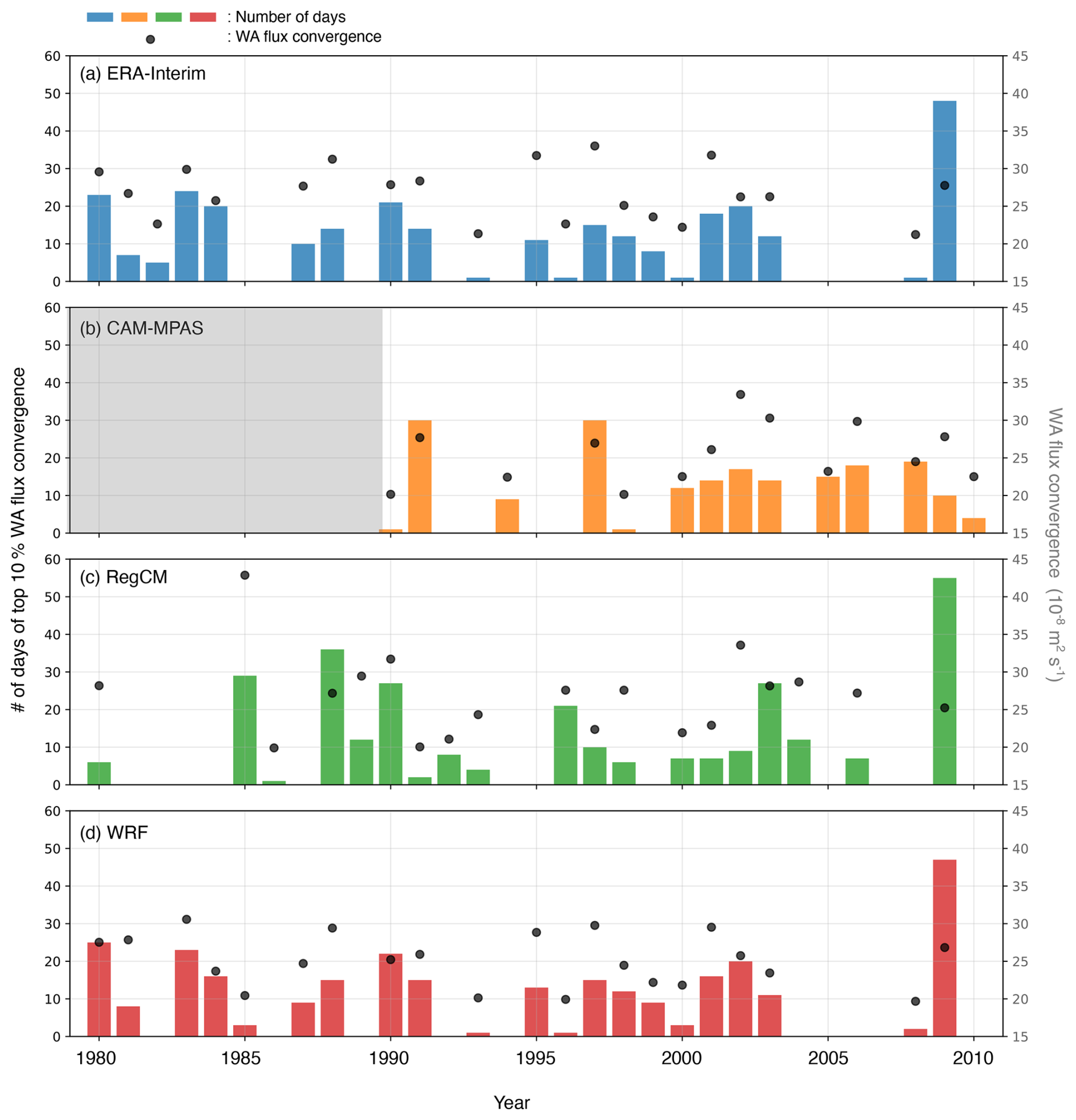
Figure B4 The bar graphs with the left y axis show the distribution of the number of days with the top 10 % strongest convergence of WA flux convergence over the West Coast area (blue boxes in Figs. 12 and 13) in (a) ERA-Interim, (b) CAM-MPAS, (c) RegCM4, and (d) WRF. The black circles represent the average magnitude of the extreme WA flux convergence in each JJA season, with the right y axis. In panel (b), the first 10 years are grayed out since CAM-MPAS data are not available for this period.

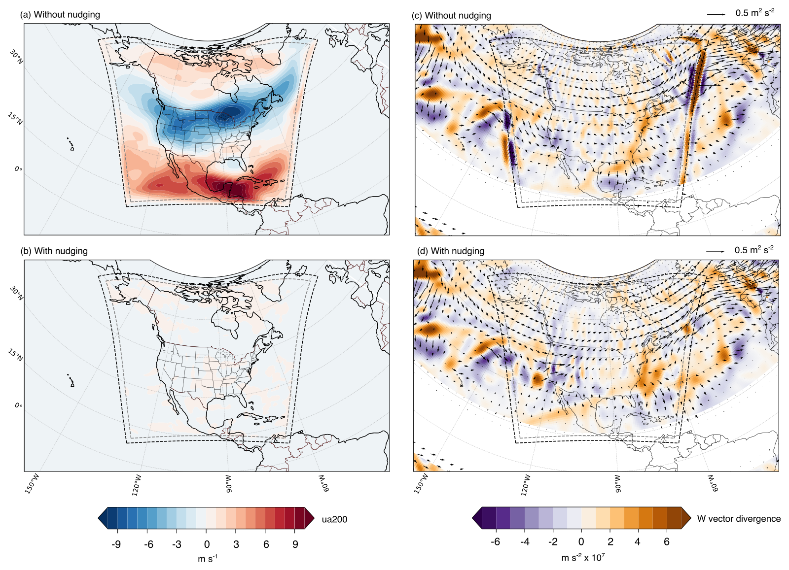
Figure B5 The effect of spectral nudging with the WRF model in the JJA-mean zonal wind bias against ERA-Interim (a, b) and horizontal component of W-vector and its divergence (c, d), all at the 200 hPa level: (a, c) without spectral nudging, (b, d) with spectral nudging. W-vector is calculated from the sensitivity simulations using the single-season JJA mean as the base state.

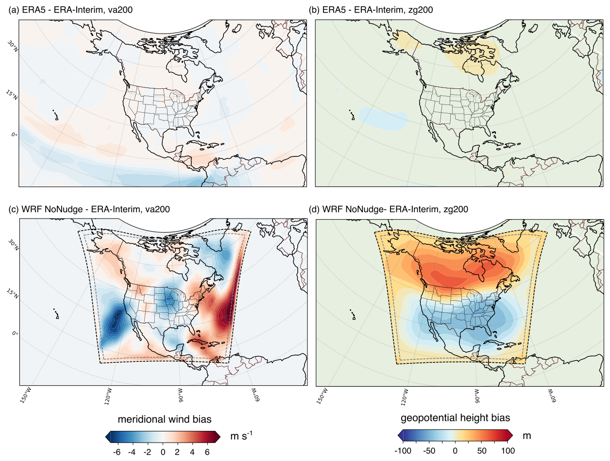
Figure B6 Differences between ERA5 and ERA-Interim in the JJA-mean (a) va200 and (b) zg200, as well as the differences between the WRF simulation without spectral nudging and ERA-Interim in (c) va200 and (d) zg200. The 1980–2010 JJA climatology is used in (a) and (b), while the 2010 JJA season only is used in (c) and (d).

B1 Lateral boundary treatment in RegCM4 and WRF

This subsection introduces the configurations of the LB buffer zone in the RegCM4 and WRF simulations for NA-CORDEX. Both models follow the LB treatment proposed by Davies (1976), with several options for the shape and coefficients of the weighting functions to blend the model-predicted values and the large-scale forcing data. The RegCM4 and WRF simulations for NA-CORDEX differ in several of those options, as summarized below from Mearns et al. (2017) and Diez-Sierra et al. (2022b).

On the outermost grid point, referred to as the specified zone in Skamarock et al. (2008), all the prognostic variables are strictly those provided from the forcing data after interpolation in time and space (Fig. B7a). The specified zone is a single grid box in both RegCM4 and WRF simulations. The next n_relax grid points constitute the relaxation zone, where additional terms are included in the prognostic equations (Eq. 6 in Giorgi et al., 1993 and Eq. 6.1 in Skamarock et al., 2008):

$$\begin{array}{}\text{(B1)}& \begin{array}{rl}{\left({\displaystyle \frac{\partial {\mathit{\alpha }}_{\mathrm{m}}}{\partial t}}\right)}_n=& (\mathrm{advection},\mathrm{source}/\mathrm{sinks},\mathrm{and}\mathrm{other}\\ & \mathrm{physical}\mathrm{terms})+\mathrm{\dots }F(n)F_{\mathrm{1}}\left({\mathit{\alpha }}_{\mathrm{f}}-{\mathit{\alpha }}_{\mathrm{m}}\right)\\ & -F\left(n\right)F_{\mathrm{2}}{\mathrm{\nabla }}^{\mathrm{2}}\left({\mathit{\alpha }}_{\mathrm{f}}-{\mathit{\alpha }}_{\mathrm{m}}\right)\end{array}\end{array}$$

where α_m and α_f are the model-simulated and forcing values for a prognostic variable α, respectively, and n is the gridbox index from the boundary (n=1 for the specified zone, and $n=n_{\mathrm{spec}}+n_{\mathrm{relax}}$ for the last grid box within the relaxation zone). In this formulation, model-predicted values are relaxed toward the external data by Newtonian relaxation (the second-to-last term) and the differences between the modeled and large-scale forcing values are smoothed by the diffusion-like term (the last term).

F₁ and F₂ are constants that depend on the timestep and grid spacing. F₁ is exactly the same in the two models as

$$F_{\mathrm{1}}={\displaystyle \frac{\mathrm{0.1}}{\mathrm{\Delta }t}}$$

where Δt denotes the model time step (s). F₂ is slightly different; RegCM4 uses the following form

$$F_{\mathrm{2}}={\displaystyle \frac{(\mathrm{\Delta }s{)}^{\mathrm{2}}}{\mathrm{50}\mathrm{\Delta }t}}$$

where Δs denotes the grid spacing (km). For WRF, it is given as

$$F_{\mathrm{2}}={\displaystyle \frac{\mathrm{1}}{\mathrm{50}\mathrm{\Delta }t}}.$$

F(n) is a weighting function that gradually reduces its magnitude from the outer-most to the inner-most grid boxes within the relaxation zone. Both RegCM4 and WRF offer the options of linear and exponential functions. The WRF simulations for NA-CORDEX use a linear weighting function with n_spec=1 and n_relax=10:

$$F\left(n\right)={\displaystyle \frac{n_{\mathrm{spec}}+n_{\mathrm{relax}}-n}{n_{\mathrm{relax}}-\mathrm{1}}}=-{\displaystyle \frac{\mathrm{11}}{\mathrm{9}}}n,$$

while the RegCM4 simulations use an exponential function:

$$F\left(n\right)=\exp \left(-{\displaystyle \frac{(n-\mathrm{2})}{N_I}}\right).$$

The coefficient N_I=N_I(z) varies with height so that the model receives stronger large-scale forcing at higher altitudes (Giorgi et al., 1993). Figure B7b shows three examples of RegCM4's exponential weight function for N_I=1, 3, 6, along with the linear function in WRF.

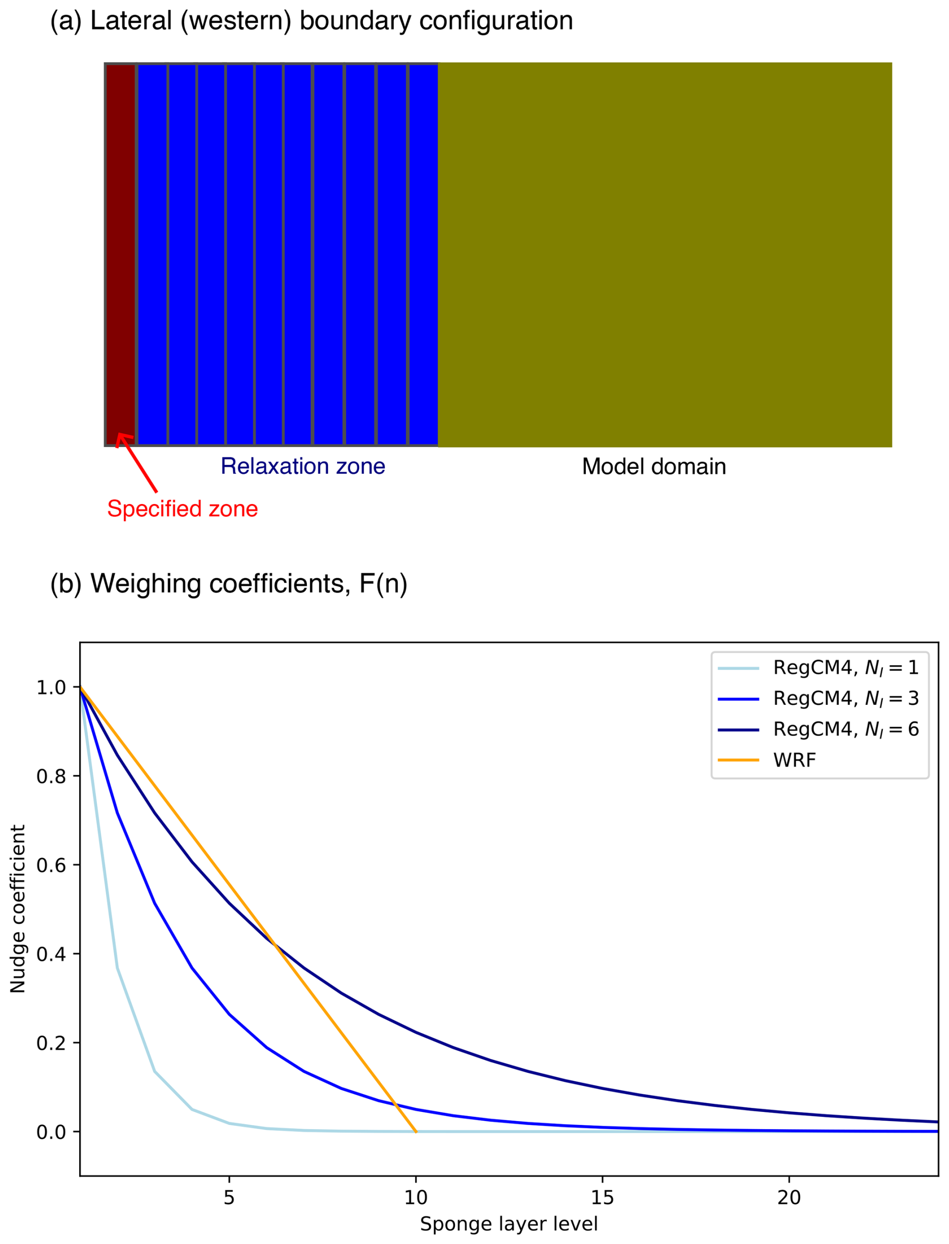
Figure B7 Illustration of the lateral boundary conditions in the RegCM4 and WRF configurations for NA-CORDEX: (a) an example configuration of specified and relaxation zones in the western boundary with n_relax=10, and (b) weighting coefficients (F(n)) in RegCM4 and WRF. Three curves are shown for RegCM4 corresponding to N_I=1, 3, 6.

Appendix C: Rossby wave

C1 Linear wave theory

We provide a brief review of the linear wave theory to help readers without a strong background in this topic understand the Rossby wave diagnostics. The materials follow Sects. 7.7 and 10.5 in Holton (2004), Chap. 6 in Vallis (2017), and more complex cases in Karoly (1983) and Li et al. (2015).

The dynamics of Rossby waves are studied in terms of the conservation law for quasi-geostrophic potential vorticity (e.g., Takaya and Nakamura, 2001; Li, 2020) since the restoring force for Rossby waves is the gradient of potential vorticity. For studying Rossby wave propagation in the atmosphere away from strong divergence, it is also common to use the vorticity equation in the barotropic atmosphere (i.e., a single layer with constant density in x and y, thus non-divergent circulations), which is:

$$\begin{array}{}\text{(C1)}& {\displaystyle \frac{\partial \mathit{\eta }}{\partial t}}+u{\displaystyle \frac{\partial \mathit{\eta }}{\partial x}}+v{\displaystyle \frac{\partial \mathit{\eta }}{\partial y}}=\mathrm{0}\end{array}$$

where η denotes the absolute vorticity $\mathit{\eta }=\mathit{\zeta }+f$, f=2Ωsin ϕ is the Coriolis parameter, and ζ is the vertical component of relative vorticity. The friction is ignored. Also, with the assumption of a non-divergent system, u and v are the zonal and meridional components of rotational winds, respectively. Strictly speaking, this single-layer (barotropic or shallow-water) vorticity equation is applicable for the middle ($<\approx \mathrm{300}$ hPa) or near the top of the troposphere ($>\approx \mathrm{150}$ hPa), where wave structure is nearly vertically uniform (equivalent barotropic) (Sardeshmukh and Hoskins, 1988; Jin and Hoskins, 1995; Holton, 2004; Neduhal et al., 2024). At the same time, one needs to consider that outflows from the tropical convective systems to excite Rossby waves, and subsequent wave propagation to the middle latitudes, take place primarily in the upper troposphere (≈100–300 hPa) (Jin and Hoskins, 1995; Neduhal et al., 2024). Our analysis of the 200 hPa level is chosen primarily for the availability of high-frequency outputs from NA-CORDEX at three pressure levels: 200, 500, and 850 hPa (CORDEX, 2009), but it seems to be a reasonable compromise.

It is also common to use streamfunction, instead of vorticity, to study Rossby waves (Chen and Chen, 1990). The vorticity budget terms are noisy and not straightforward to visually interpret (Kang and Held, 1986). Streamfunction is a scalar from which rotational winds are obtained by differentiation:

$$\begin{array}{}\text{(C2)}& \begin{array}{rl}& u=-{\displaystyle \frac{\partial \mathit{\psi }}{\partial y}}\\ & v={\displaystyle \frac{\partial \mathit{\psi }}{\partial x}},\end{array}\end{array}$$

and we can write vorticity in terms of streamfunction

$$\begin{array}{}\text{(C3)}& \begin{array}{rl}\mathit{\zeta }& ={\displaystyle \frac{\partial v}{\partial x}}-{\displaystyle \frac{\partial u}{\partial y}}\\ & ={\displaystyle \frac{{\partial }^{\mathrm{2}}\mathit{\psi }}{\partial x^{\mathrm{2}}}}+{\displaystyle \frac{{\partial }^{\mathrm{2}}\mathit{\psi }}{\partial y^{\mathrm{2}}}}={\mathrm{\nabla }}^{\mathrm{2}}\mathit{\psi }.\end{array}\end{array}$$

Then Eq. (C1) becomes:

$$\begin{array}{}\text{(C4)}& \left({\displaystyle \frac{\partial }{\partial t}}+u{\displaystyle \frac{\partial }{\partial x}}+v{\displaystyle \frac{\partial }{\partial y}}\right)\left({\mathrm{\nabla }}^{\mathrm{2}}\mathit{\psi }+f\right)=\mathrm{0}.\end{array}$$

All the diagnostics we use are based on a linear perturbation framework, in which Rossby waves are defined as small perturbations (a^′) from the background (mean) state ($\stackrel{\mathrm{‾}}{a}$):

$$\begin{array}{}\text{(C5)}& \begin{array}{rl}& u=\stackrel{\mathrm{‾}}{u}+u^{\prime }\\ & v=\stackrel{\mathrm{‾}}{v}+v^{\prime }\\ & \mathit{\psi }=\stackrel{\mathrm{‾}}{\mathit{\psi }}+{\mathit{\psi }}^{\prime }\\ & \mathit{\zeta }=\stackrel{\mathrm{‾}}{\mathit{\zeta }}+{\mathit{\zeta }}^{\prime }\\ & \stackrel{\mathrm{‾}}{\mathit{\eta }}=\stackrel{\mathrm{‾}}{\mathit{\zeta }}+f={\mathrm{\nabla }}^{\mathrm{2}}\stackrel{\mathrm{‾}}{\mathit{\psi }}+f\end{array}\end{array}$$

then Eq. (C4) becomes:

$$\begin{array}{}\text{(C6)}& {\displaystyle }\begin{array}{rl}\left({\displaystyle \frac{\partial }{\partial t}}\right.& \left.+\stackrel{\mathrm{‾}}{u}{\displaystyle \frac{\partial }{\partial x}}+\stackrel{\mathrm{‾}}{v}{\displaystyle \frac{\partial }{\partial y}}\right){\mathrm{\nabla }}^{\mathrm{2}}{\mathit{\psi }}^{\prime }+u^{\prime }{\displaystyle \frac{\partial {\mathrm{\nabla }}^{\mathrm{2}}\stackrel{\mathrm{‾}}{\mathit{\psi }}+f}{\partial x}}\\ & +v^{\prime }{\displaystyle \frac{\partial {\mathrm{\nabla }}^{\mathrm{2}}\stackrel{\mathrm{‾}}{\mathit{\psi }}+f}{\partial y}}=\mathrm{0}\end{array}\text{(C7)}& {\displaystyle }\left({\displaystyle \frac{\partial }{\partial t}}+\stackrel{\mathrm{‾}}{u}{\displaystyle \frac{\partial }{\partial x}}+\stackrel{\mathrm{‾}}{v}{\displaystyle \frac{\partial }{\partial y}}\right){\mathrm{\nabla }}^{\mathrm{2}}{\mathit{\psi }}^{\prime }-{\displaystyle \frac{\partial {\mathit{\psi }}^{\prime }}{\partial y}}{\displaystyle \frac{\partial \stackrel{\mathrm{‾}}{\mathit{\eta }}}{\partial x}}+{\displaystyle \frac{\partial {\mathit{\psi }}^{\prime }}{\partial x}}{\displaystyle \frac{\partial \stackrel{\mathrm{‾}}{\mathit{\eta }}}{\partial y}}=\mathrm{0}.\end{array}$$

To study Rossby wave propagation from the source, those equations must be written in spherical coordinates or another coordinate system to account for the Earth's spherical geometry. Here, we use simple Cartesian coordinates and refer readers to previous studies for the equation in the appropriate coordinates (e.g., Hoskins and Karoly, 1981; Li et al., 2015). This partial differential equation for ψ^′ has parameters that vary in space, which prevents us from solving it analytically. To obtain an approximate analytical solution, we assume the mean state varies much more slowly than the wave disturbances, thus treating the mean state as constant locally (WKB approximation), and also assume plane wave solutions in the form of:

$$\begin{array}{}\text{(C8)}& {\mathit{\psi }}^{\prime }=A(T,X,Y)\exp \left[i\right(kx+ly-\mathit{\omega }t\left)\right]\end{array}$$

where T, X, and Y are the base-state coordinates with substantially larger scales of variations than those for the waves (t, x, y). A is the amplitude, ω is the angular frequency, k is the zonal wavenumber, and l is the meridional wavenumber (Fig. C1). A is a function of time and space. By substituting Eq. (C8) to EQ. (C6) while ignoring the variations of the base state, we can obtain the following dispersion relation [those and following equations can be found in Karoly, 1983; Takaya and Nakamura, 2001; Li et al., 2015]:

$$\begin{array}{}\text{(C9)}& \mathit{\omega }=\stackrel{\mathrm{‾}}{u}k+\stackrel{\mathrm{‾}}{v}l+{\displaystyle \frac{{\stackrel{\mathrm{‾}}{\mathit{\eta }}}_{x}l-{\stackrel{\mathrm{‾}}{\mathit{\eta }}}_{y}k}{k^{\mathrm{2}}+l^{\mathrm{2}}}}\end{array}$$

where we have used subscripts x and y to denote partial differentiation with respect to x and y. Rearranging Eq. (C9), we define the total wavenumber

$$\begin{array}{}\text{(C10)}& K^{\mathrm{2}}=k^{\mathrm{2}}+l^{\mathrm{2}}={\displaystyle \frac{{\stackrel{\mathrm{‾}}{\mathit{\eta }}}_{y}k-{\stackrel{\mathrm{‾}}{\mathit{\eta }}}_{x}l}{\stackrel{\mathrm{‾}}{u}k+\stackrel{\mathrm{‾}}{v}l-\mathit{\omega }}}.\end{array}$$

For stationary waves with ω=0, the total wavenumber is

$$\begin{array}{}\text{(C11)}& K^{\mathrm{2}}=k^{\mathrm{2}}+l^{\mathrm{2}}={\displaystyle \frac{{\stackrel{\mathrm{‾}}{\mathit{\eta }}}_{y}k-{\stackrel{\mathrm{‾}}{\mathit{\eta }}}_{x}l}{\stackrel{\mathrm{‾}}{u}k+\stackrel{\mathrm{‾}}{v}l}}.\end{array}$$

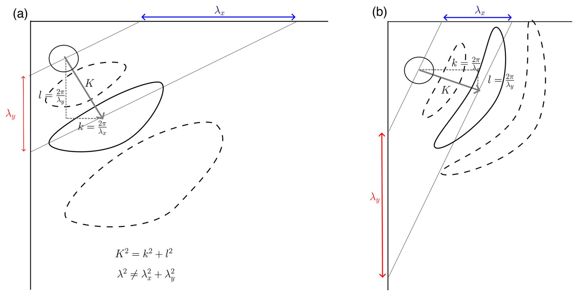
Figure C1 Schematics to clarify the wavenumbers and wavelengths with two example cases: (a) zonal and meridional wavelengths are similar, and (b) meridional wavelength is longer than the zonal wavelength.

The x and y components of group velocity are obtained from the dispersion relationship (with the quotient rule of differentiation):

$$\begin{array}{}\text{(C12)}& \begin{array}{rl}& u_{\mathrm{g}}={\displaystyle \frac{\partial \mathit{\omega }}{\partial k}}=\stackrel{\mathrm{‾}}{u}+{\displaystyle \frac{\left(\left(k^{\mathrm{2}}-l^{\mathrm{2}}\right){\stackrel{\mathrm{‾}}{\mathit{\eta }}}_y-\mathrm{2}kl{\stackrel{\mathrm{‾}}{\mathit{\eta }}}_x\right)}{K^{\mathrm{4}}}}\\ & v_{\mathrm{g}}={\displaystyle \frac{\partial \mathit{\omega }}{\partial l}}=\stackrel{\mathrm{‾}}{v}+{\displaystyle \frac{\mathrm{2}kl{\stackrel{\mathrm{‾}}{\mathit{\eta }}}_y+\left(k^{\mathrm{2}}-l^{\mathrm{2}}\right){\stackrel{\mathrm{‾}}{\mathit{\eta }}}_x}{K^{\mathrm{4}}}}.\end{array}\end{array}$$

The time evolution of wavenumbers is governed by the conservation of the number of waves (Whitham, 1960), accounting for the spatial variation of the base state (rather than ignoring it, as in the previous derivation of the dispersion relationship). Accordingly, the derivatives of ω with respect to the large-scale coordinates (X, Y) determine the time rate of change of the wavenumbers k and l as the wave packet moves along the group velocity,

$$\begin{array}{}\text{(C13)}& {\displaystyle }& {\displaystyle \frac{{\mathrm{d}}_{\mathrm{g}}k}{\mathrm{d}T}}=-{\displaystyle \frac{\partial \mathit{\omega }}{\partial X}}=-k{\displaystyle \frac{\partial \stackrel{\mathrm{‾}}{u}}{\partial X}}-l{\displaystyle \frac{\partial \stackrel{\mathrm{‾}}{v}}{\partial X}}-{\displaystyle \frac{\mathrm{1}}{K^{\mathrm{2}}}}\left(l{\displaystyle \frac{\partial {\stackrel{\mathrm{‾}}{\mathit{\eta }}}_x}{\partial X}}-k{\displaystyle \frac{\partial {\stackrel{\mathrm{‾}}{\mathit{\eta }}}_y}{\partial X}}\right)\text{(C14)}& {\displaystyle }& {\displaystyle \frac{{\mathrm{d}}_{\mathrm{g}}l}{\mathrm{d}T}}=-{\displaystyle \frac{\partial \mathit{\omega }}{\partial Y}}=-k{\displaystyle \frac{\partial \stackrel{\mathrm{‾}}{u}}{\partial Y}}-l{\displaystyle \frac{\partial \stackrel{\mathrm{‾}}{v}}{\partial Y}}-{\displaystyle \frac{\mathrm{1}}{K^{\mathrm{2}}}}\left(l{\displaystyle \frac{\partial {\stackrel{\mathrm{‾}}{\mathit{\eta }}}_x}{\partial Y}}-k{\displaystyle \frac{\partial {\stackrel{\mathrm{‾}}{\mathit{\eta }}}_y}{\partial Y}}\right)\end{array}$$

(these are same as Eqs. 1 and 2, but repeated here). Equations (C13) and (C14) show that the base state wind shear changes the shape and scale of the wave (i.e., k and l) as the wave travels at the group velocity.

If the background (mean) circulations are represented by the zonal mean zonal winds (constant over longitudes) and zero meridional winds, then the dispersion relationship is

$$\begin{array}{}\text{(C15)}& \mathit{\omega }=\stackrel{\mathrm{‾}}{u}k-{\displaystyle \frac{{\stackrel{\mathrm{‾}}{\mathit{\eta }}}_{y}k}{k^{\mathrm{2}}+l^{\mathrm{2}}}}\end{array}$$

and the group velocities are given by:

$$\begin{array}{}\text{(C16)}& \begin{array}{rl}& u_{\mathrm{g}}=\stackrel{\mathrm{‾}}{u}+{\displaystyle \frac{\mathrm{2}{\stackrel{\mathrm{‾}}{\mathit{\eta }}}_y{k}^{\mathrm{2}}}{K^{\mathrm{2}}}}\\ & v_{\mathrm{g}}={\displaystyle \frac{\mathrm{2}{\stackrel{\mathrm{‾}}{\mathit{\eta }}}_{y}kl}{K^{\mathrm{2}}}}.\end{array}\end{array}$$

For stationary waves ω=0 in this zonally uniform background case, we have a stationary wavenumber as

$$K_{\mathrm{s}}^{\mathrm{2}}={\displaystyle \frac{{\stackrel{\mathrm{‾}}{\mathit{\eta }}}_y}{\stackrel{\mathrm{‾}}{u}}},$$

which is the same as Eq. (4) in the main text. In this simpler case, the total wavenumber depends on only two quantities: the meridional gradient of the background absolute vorticity and the background zonal wind. When either is negative, K_s is an imaginary number. In this case, instead of oscillating in space, the wave solution becomes evanescent, decaying exponentially with distance (Eq. C8); hence, Rossby waves do not propagate over such a region.

For a zonally uniform background state, Eq. (C13) suggests $\frac{\partial \mathit{\omega }}{\partial X}=\mathrm{0}=\frac{{\mathrm{d}}_{\mathrm{g}}k}{\mathrm{d}T}$, so k remains the same as given at the initial time k₀, while l (hence K_s) evolves as the wavepacket travels through the background state. Changes in l along the path are related to the meridional propagation of wave packets (l is the y component of the wavenumber vector, Fig. C1). Writing l as:

$$\begin{array}{}\text{(C17)}& l=\pm \sqrt{K_{\mathrm{s}}^{\mathrm{2}}-k_{\mathrm{0}}^{\mathrm{2}}},\end{array}$$

we can see: (1) where K_s is large and K_s≫k₀, l is real and large, thus Rossby waves can propagate meridionally with smaller meridional wavelengths, (2) where K_s≈k₀, l becomes small, the wave fronts become oriented North–South, and the wave energy travels almost purely zonally (Fig. C1b), and (3) where K_s=k₀, l=0, and the wave cannot propagate any further meridionally, and turn back toward higher K_s (turning latitude). If a Rossby wave is excited within the local maximum of K_s with a sufficient latitudinal width, then the wave is trapped within the latitude band and propagates zonally since the strong gradients to the north and south refract back the waves.

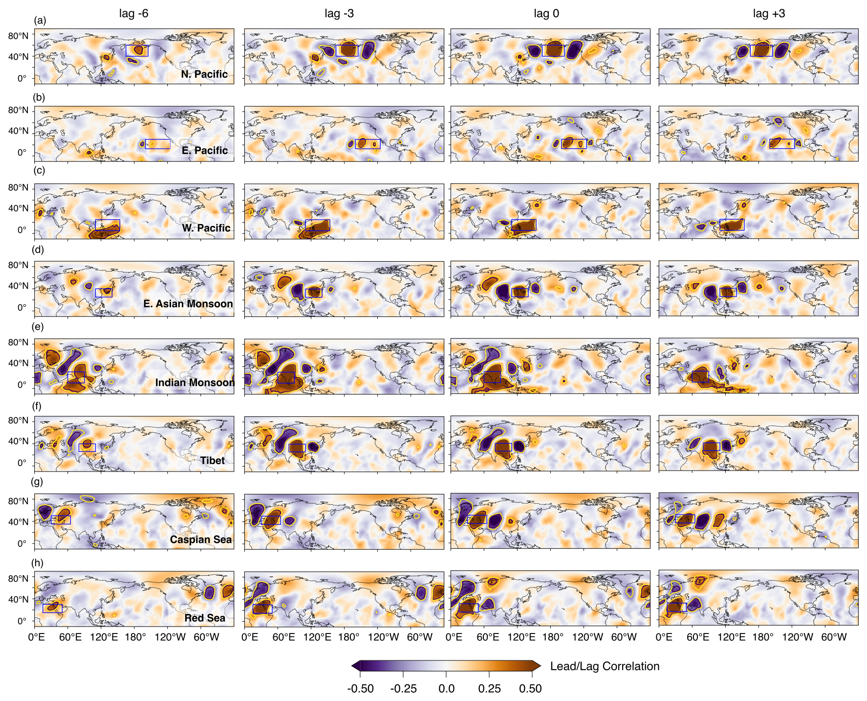
Figure C2 Lead/lag correlation between the band-passed perturbation meridional winds at the 200 hPa level (va200^′) averaged over the source regions (denoted by the blue rectangles) and all the other grid points. Each row represents different source locations: (a) North Pacific, (b) East Pacific, (c) West Pacific, (d) East Asian Monsoon, (e) Indian Monsoon, (f) Tibetan Plateau, (g) Caspian Sea, and (h) Red Sea.

In Fig. 7a, we apply this metric to each grid point, assuming that the metric K_s is locally applicable; this is commonly done and able to provide a qualitative picture of the preferred wave pathways (Hoskins and Ambrizzi, 1993). An example of turning latitude is the north/south of the mid-latitude jet over the Pacific, where K_s is becoming smaller toward the inhibited region. To the south of the subtropical jet, zonal winds are tending to zero, changing from westerly to easterly (Fig. 5a). This makes K_s increase toward infinity, or the wavelength tends toward zero, implying that the waves break and mix into the background flow. Also, the group velocity decreases toward zero with increasing K_s (Eq. C16), thereby prohibiting wave propagation. This is called critical latitude.

C2 Sources of Rossby waves propagating to North America

To apply ray tracing in Sect. 3.3, it is necessary to specify the locations of the wave sources. Following previous studies, we used lead/lag correlation maps of the daily-mean meridional perturbation winds, va200^′, using the same background state and the perturbation winds for the W-vector diagnosis. The base point is placed in one of the eight source regions: North Pacific, East Pacific, West Pacific, East Asian Monsoon, Indian Monsoon, Tibetan Plateau, Caspian Sea, and Red Sea. The time series of va200^′ after area-averaging over the base location (indicated by the box in Fig. C2) is correlated to the same variables at all the other grid points, varying the lags from −15 to +15 d.

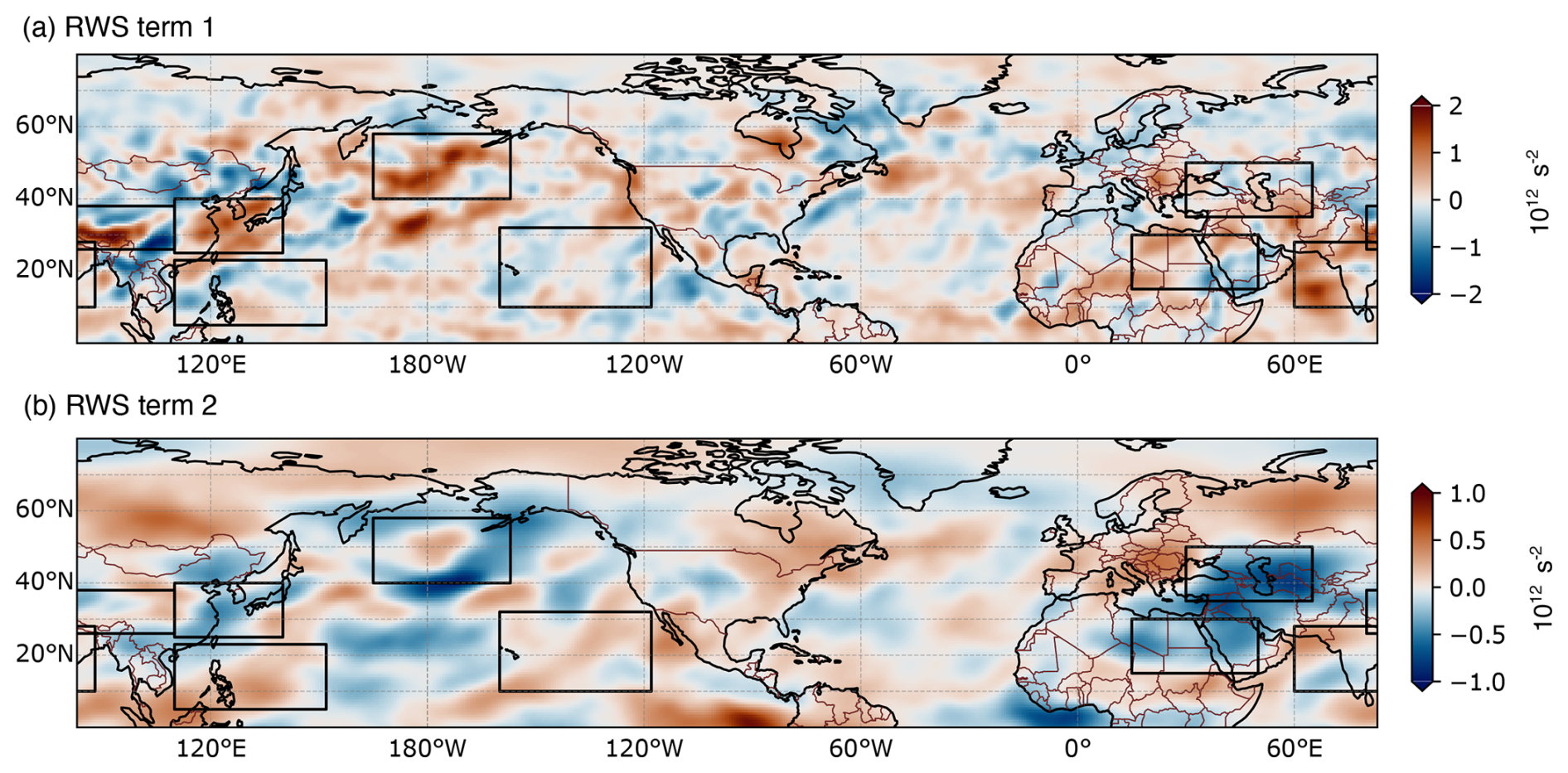
Figure C3 The first (a) and second (b) terms in the Rossby wave source (Eq. C19) calculated from ERA Interim.

Among the eight source locations examined, statistically significant correlations in the grid points over North America are found for the North Pacific and East Pacific (Fig. C2a and b), suggesting that those two are the critical wave sources for quasi-stationary Rossby waves traveling to North America. However, the figure indicates other indirect wave sources from which wave signals reach those two sources. For example, from the East Asian Monsoon region (Fig. C2d), statistically significant signals first appear to its west. The signal becomes stronger over 3 d, such that a statistically significant correlation links the East Asian region to Europe with a lag of −3. Then the signal in the downwind direction becomes strong and significant, reaching the North Pacific source region and almost the West Coast of North America (lags 0 and 3). Meanwhile, the wave signals from the Caspian Sea reach East Asia. A dipole wave pattern first establishes 6 d earlier (from day 0) over the Caspian Sea and Europe (Fig. C2g, lag −6). Three days later (lag −3), another negative phase appears to the east, then another positive phase over China, reaching the East Asian Monsoon source.

Sardeshmukh and Hoskins (1988) suggested another diagnostic for Rossby wave sources. They linearized Eq. (C1) to solve for the time tendency of perturbation absolute vorticity to identify the source terms. Doing so, they suggested to partition the winds into rotational (v_Ψ) and divergent (v_χ) components when diagnosing Rossby wave sources, particularly in the tropics, so that one does not overlook the contribution of vorticity advection by the divergent winds:

$$\begin{array}{}\text{(C18)}& {\displaystyle \frac{\partial \mathit{\eta }}{\partial t}}+{\mathbf{v}}_{\mathrm{\Psi }}\cdot \mathrm{\nabla }\mathit{\eta }=-{\mathbf{v}}_{\mathit{\chi }}\cdot \mathrm{\nabla }\mathit{\eta }-\mathit{\eta }\left(\mathrm{\nabla }\cdot {\mathbf{v}}_{\mathit{\chi }}\right),\end{array}$$

where advection by the rotational and divergent winds is separated, and the latter is moved to the right-hand side as a forcing. Linearizing the equation, we have:

$$\begin{array}{}\text{(C19)}& \begin{array}{rl}{\displaystyle \frac{\partial {\mathit{\eta }}^{\prime }}{\partial t}}& +{\stackrel{\mathrm{‾}}{\mathbf{v}}}_{\mathrm{\Psi }}\cdot \mathrm{\nabla }{\mathit{\eta }}^{\prime }+{\mathbf{v}}_{\mathrm{\Psi }}^{\prime }\cdot \mathrm{\nabla }\stackrel{\mathrm{‾}}{\mathit{\eta }}=-\mathrm{\nabla }\cdot \left({\mathbf{v}}_{\mathit{\chi }}^{\prime }\stackrel{\mathrm{‾}}{\mathit{\eta }}\right)-\mathrm{\nabla }\cdot \left({\stackrel{\mathrm{‾}}{\mathbf{v}}}_{\mathit{\chi }}{\mathit{\eta }}^{\prime }\right)\\ & =-\stackrel{\mathrm{‾}}{\mathit{\eta }}\left(\mathrm{\nabla }\cdot {\mathbf{v}}_{\mathit{\chi }}^{\prime }\right)-{\mathbf{v}}_{\mathit{\chi }}^{\prime }\cdot \mathrm{\nabla }\stackrel{\mathrm{‾}}{\mathit{\eta }}-{\mathit{\eta }}^{\prime }\left(\mathrm{\nabla }\cdot {\stackrel{\mathrm{‾}}{\mathbf{v}}}_{\mathit{\chi }}\right)-{\stackrel{\mathrm{‾}}{\mathbf{v}}}_{\mathit{\chi }}\cdot \mathrm{\nabla }{\mathit{\eta }}^{\prime }.\end{array}\end{array}$$

The left-hand side is the change of the perturbation absolute vorticity following the rotational winds. The right-hand side now has four terms: the first and third are stretching of the mean and perturbation vorticities by the perturbation and mean divergence, respectively. The second and fourth terms are the advection of the mean and perturbation vorticity by the perturbation and mean divergent winds, respectively. The right-hand-side terms are referred to as the Rossby Wave Source (RWS) (S^′). Note that here RWS is defined for the perturbation vorticity, not the mean vorticity. Lin (2009) found the first two terms in the second line in Eq. (C19) dominate other source terms. These are shown in Fig. C3, showing that all the source regions mentioned above exhibit strong magnitudes of either source term.

C3 W vector

Based on the Eqs. (C2), (C3), and (C5), the horizontal component of the wave activity flux by TN01, or the “W-vector” are written as:

$$\begin{array}{c}{\displaystyle }\begin{array}{rl}{\mathit{W}}_x& ={\displaystyle \frac{\mathrm{1}}{\mathrm{2}\left|\mathbf{V}\right|}}\left[\stackrel{\mathrm{‾}}{u}\left({\displaystyle \frac{\partial {{\mathit{\psi }}^{\prime }}^{\mathrm{2}}}{\partial x}}-{\mathit{\psi }}^{\prime }{\displaystyle \frac{{\partial }^{\mathrm{2}}{\mathit{\psi }}^{\prime }}{\partial x^{\mathrm{2}}}}\right)\right.\\ & \left.+\stackrel{\mathrm{‾}}{v}\left({\displaystyle \frac{\partial {\mathit{\psi }}^{\prime }}{\partial x}}{\displaystyle \frac{\partial {\mathit{\psi }}^{\prime }}{\partial y}}-{\mathit{\psi }}^{\prime }{\displaystyle \frac{{\partial }^{\mathrm{2}}{\mathit{\psi }}^{\prime }}{\partial x\partial y}}\right)\right]+{\displaystyle \frac{\stackrel{\mathrm{‾}}{u}}{\left|\mathbf{V}\right|}}{C}_{\mathrm{p}}M\end{array}\\ \text{(C20)}& {\displaystyle }\begin{array}{rl}{\mathit{W}}_y& ={\displaystyle \frac{\mathrm{1}}{\mathrm{2}\left|\mathbf{V}\right|}}\left[\stackrel{\mathrm{‾}}{u}\left({\displaystyle \frac{\partial {\mathit{\psi }}^{\prime }}{\partial x}}{\displaystyle \frac{\partial {\mathit{\psi }}^{\prime }}{\partial y}}-{\mathit{\psi }}^{\prime }{\displaystyle \frac{{\partial }^{\mathrm{2}}{\mathit{\psi }}^{\prime }}{\partial x\partial y}}\right)\right.\\ & \left.+\stackrel{\mathrm{‾}}{v}\left({\displaystyle \frac{\partial {{\mathit{\psi }}^{\prime }}^{\mathrm{2}}}{\partial y}}-{\mathit{\psi }}^{\prime }{\displaystyle \frac{{\partial }^{\mathrm{2}}{\mathit{\psi }}^{\prime }}{\partial y^{\mathrm{2}}}}\right)\right]+{\displaystyle \frac{\stackrel{\mathrm{‾}}{v}}{\left|\mathbf{V}\right|}}{C}_{\mathrm{p}}M\end{array}\end{array}$$

where $\left|\mathbf{V}\right|=\sqrt{{\stackrel{\mathrm{‾}}{u}}^{\mathrm{2}}+{\stackrel{\mathrm{‾}}{v}}^{\mathrm{2}}}$ and C_p is the wave phase speed. The last term represents the wave activity flux at the phase velocity along the background wind vector. This is the form of W-vector on the pressure coordinate (Eq. C5 in TN01). Here, the mean winds ($\stackrel{\mathrm{‾}}{u}$ and $\stackrel{\mathrm{‾}}{v}$) are the time-mean geostrophic winds, and the perturbation winds (and the associated streamfunction: u^′, v^′ and ψ^′) are the deviation of geostrophic winds from the mean winds. We set C_p=0 for quasi-stationary waves.