MeteoSaver v1.0: a machine-learning based software for the transcription of historical weather data

Archives of observed weather data present unique opportunities for scientists to obtain long time series of the historical climate for many regions of the world. Unfortunately, most of these observational records are to-date available only on paper, and thus require digitization and transcription to facilitate analysis of climatic trends. Here we present a new open-source software, MeteoSaver, that uses machine learning (ML) algorithms to transcribe handwritten records of historical weather data. MeteoSaver version 1.0 processes images of tabular sheets alongside user-defined configuration settings, performing transcription through five sequential steps: (i) image pre-processing, (ii) table and cell detection, (iii) transcription, (iv) quality assessment and quality control, and (v) data formatting and upload. As an illustration and evaluation of the software, we apply MeteoSaver to ten pictured sheets of handwritten temperature and precipitation observations from the Democratic Republic of the Congo. The results show that 95 %–100 % of the daily temperature values can be transcribed, of which a median of 74.4 % reached the highest internal quality flag and 74 % matches with the manually transcribed record, yielding a median mean absolute error of 0.3 °C. These results illustrate that MeteoSaver can be applied to a range of handwriting styles and varying tabular dimensions, paper sizes, and maintenance conditions, highlighting its potential for transcribing tabular meteorological observations from multiple regions, especially if the sheets have a consistent format. Overall, our open-source software can help address the challenges of limited available hydroclimatic data within many regions of the world, by helping to save millions of handwritten records of historical weather data presently stored in archives, and expedite research on the climate and environmental changes in data scarce regions.

1 Introduction

Today, access to in-situ meteorological data is more crucial than ever in order to comprehend our globe's climate variability and the effects of climate change. These observational datasets are key for: (i) gaining process understanding of components within the climate system (IPCC, 2021; Roberts et al., 2018), (ii) calibrating satellite data (Funk et al., 2015; Huffman et al., 2023; Adler et al., 2018), (iii) constraining reanalysis products (Hersbach et al., 2020; Bell et al., 2021; Kalnay et al., 1996), (iv) evaluation and improvement of climate models (Flato et al., 2013; Braverman et al., 2017), and (v) constraining uncertainties in future climate projections (Eyring et al., 2019), among others.

However, the availability of in-situ meteorological data is limited in many regions, particularly in the Global South, which poses a significant challenge to these efforts (Xu et al., 2014; IPCC, 2021; Seneviratne et al., 2021). As a result, gridded products for meteorological data often lack sufficient data for regions in the Global South. For example, Shaman (2014) reports that less than 40 stations across Central Africa were employed in the development of the University of East Anglia – Climate Research Unit (CRU) TS3.10 gridded surface temperature dataset for the period 1976–2012, for an area of approximately 3×10⁶ km². Similarly, only 353 stations across the entire South American continent provided surface temperature data to the Global Historical Climatology Network (GHCN-V3) for the period 1951–2011, which is a gridded climate product of the US National Climatic Data Center (Xu et al., 2014). This absence of sufficient in-situ data often leads to inconclusive statements about how climate change is affecting these regions. For example, Central Africa and Southern South America are the only regions where the Intergovernmental Panel on Climate Change (IPCC) has not reported any observed changes in hot extremes or attributed these changes to anthropogenic activities, due to the scarcity of in-situ data (IPCC, 2021; Seneviratne et al., 2021). Moreover, for the same reason, observed changes in heavy precipitation since the 1950s remain unreported for much of Central and South America, as well as Central and East Africa (IPCC, 2021; Seneviratne et al., 2021). Similarly, a recent study by World Weather Attribution highlighted how insufficient historical weather data hindered the assessment of climate change's role in the catastrophic 2023 Lake Kivu floods, which resulted in over 500 deaths in the Democratic Republic of Congo (DRC) and Rwanda (Kimutai et al., 2023). As climate change escalates, the need for reliable historical weather records becomes ever larger. These records are essential not only for scientific research but also for informing discussions on loss and damage by strengthening evidence from attribution research (Noy et al., 2023). This is particularly crucial as losses and damages are projected to rise with climate change, becoming more concentrated in developing countries across the Global South (IPCC, 2022), where current capacity to carry out attribution studies is currently limited by data availability (Otto et al., 2020; King et al., 2023).

In many regions of the world, millions of daily weather records, such as precipitation and temperature records from various stations are still stored in hard copies within archives (e.g. Hawkins et al., 2022, 2023; Brönnimann et al., 2018; Noone et al., 2024). For instance, until 2021, 4 million copies of meteorological records collected from 44 African countries through the African Centre of Meteorological Applications for Development (ACMAD) initiative were stored by the Royal Meteorological Institute of Belgium (RMI) solely in microfilm and microfiche formats (Noone et al., 2024). Additionally, Brönnimann et al. (2018) reports the existence of partially explored archives in countries such as Finland, Sweden, Denmark, France, and Portugal, among others, which still hold ship logs in hard copy. These logs contain meteorological data, such as barometric pressure, recorded along ship routes, including those in the Southern Hemisphere, where data availability remains particularly scarce (Brönnimann et al., 2018; Wilkinson and Vasquez, 2017; Jourdain et al., 2015). These extensive records of observed weather, present valuable opportunities to address the challenges of limited observations, and understanding of our climate variability, by providing long time series of historical climate data for many regions of the world. For example, Hawkins et al. (2023) demonstrates how rescued atmospheric pressure observations from archived data by the UK Met Office and Scottish Meteorological Society were assimilated into the reanalysis of Storm Ulysses, a severe windstorm that occurred in 1903. This significantly improved the reconstruction of the event and the estimation of risks associated with similar windstorms (Hawkins et al., 2023). Moreover, on a broader scale, it demonstrated the value of archived weather data in enhancing the accuracy of extreme event reconstructions and understanding present-day risks (Hawkins et al., 2023; Brönnimann et al., 2018), further underscoring the need for data rescue projects.

According to the World Meteorological Organization (WMO), data rescue involves all efforts to access, catalog and preserve data at risk of being lost by converting these historical hard copy records into digital and/or machine-readable formats (WMO, 2024). These data rescue projects are typically divided into two stages: digitization and transcription. The digitization stage involves organising and imaging (scanning) the hard copy records, as well as saving their corresponding metadata (WMO, 2024). This ensures easy identification and retrieval of the digital data copies. The transcription stage then involves converting the data from these digital copies into machine-readable formats, such as spreadsheets, ready for analysis. Currently, 139 past and ongoing data rescue projects from various parts of the world are reported on the Data Rescue Portal, operated by the WMO and the Copernicus Climate Change Service (C3S) (Copernicus Climate Change Service, 2024). A successful example of these data rescue projects is the recently completed WeatherRescue.org initiative, which digitized and transcribed over 3 million daily weather observations, including atmospheric pressure, precipitation, and temperature, recorded in the Scottish Highlands between 1883–1910 (Hawkins et al., 2019; Copernicus Climate Change Service, 2024). Following this, the data was uploaded to open-access repositories through the C3S, helping to fill gaps in the region's historical climate record (Hawkins et al., 2019). A second example is the digitization and transcription of approximately 5 million weather observations recorded between 1861–1919 in Southern Poland, sourced from the archives of the Institute of Meteorology and Water Management (Wypych et al., 2024). This rescued data was key in the study by Wypych et al. (2024), which highlighted climate variability in the Małopolska region. This project also underscored the urgent need to digitize archived in-situ data, as many weather records in these archives had deteriorated significantly, making parts of the recorded data unrecognizable and difficult to transcribe, resulting in the loss of valuable information (Wypych et al., 2024).

Brönnimann et al. (2018) points out that one of the major challenges in data rescue projects is the transcription process. Many projects tend to halt after the digitization phase, leaving the transcription to be completed at a later stage (Brönnimann et al., 2018). This is because traditional transcription relies on manual efforts, where observations in the images or scans from the digitization phase, are keyed into a spreadsheet or standardized format by hand (e.g. Wypych et al., 2024; Latapy et al., 2022). This process is labor-intensive and time-consuming, as transcribing large data collections can require numerous man-years of effort (Hawkins et al., 2022). Recently, the involvement of citizen scientists, on platforms such as Zooniverse, in transcribing historical weather data from images to digital form has proven more efficient, significantly reducing the person-years required to complete transcription projects, with some projects even mobilizing thousands of volunteers (e.g. Hawkins et al., 2019, 2022; Craig and Hawkins, 2020). However, the success of these citizen science projects relies on effective mobilization factors such as media coverage, volunteer availability and willingness, ongoing engagement, and thorough preparation of the images for upload to the platforms (Hawkins et al., 2022). More recently, several efforts have been made to integrate the transcription into classroom-based assessments (e.g. Noone et al., 2024), but these initiatives have almost exclusively been limited to university settings and have not yet cracked transcription at speed and scale.

An emerging approach to addressing the challenges of transcription involves using Artificial Intelligence/Machine Learning (AI/ML) algorithms. This approach harnesses the power of computer vision algorithms and Optical Character Recognition/Handwritten Text Recognition (OCR/HTR) models to transcribe large datasets more efficiently and quickly (Vercruysse et al., 2025; Nockels et al., 2022). For example, in the field of Digital Humanities, OCR/HTR tools have been explored to expedite and reduce the cost of transcribing vast collections of historical texts and documents in libraries and archives (Nockels et al., 2022; Terras, 2022; Sánchez et al., 2014). A notable case is the recent transcription of over 3 million pages of historical texts from the National Archives of the Netherlands using Transkribus HTR models (Transkribus, 2024). However, despite being suggested by numerous studies (e.g. Bradshaw et al., 2015; Latapy et al., 2022), these AI/ML approaches for transcribing historical meteorological data have not been extensively explored. Bradshaw et al. (2015) highlights that the current models used for transcribing historical texts or pages would need to be adapted to effectively transcribe historical meteorological data, which is often presented in tabular or ledger format. Vercruysse et al. (2025) demonstrates that commercial transcription software like Transkribus and Amazon Textract currently offer more advanced text recognition models compared to open-source alternatives such as Tesseract and Pylaia, and they also include table structure detection. However, transcribing large volumes of data with these commercial tools would be very costly (Vercruysse et al., 2025). Therefore, there is a need to further train and improve open-source transcription models, not only as a cost-effective solution but also to uphold the principles of Open Science in transcribing historical meteorological data (Vercruysse et al., 2025).

To help overcome these challenges, we here present an ML based open source software, MeteoSaver, used here for the transcription of the digitized data to machine readable format. We illustrate the functionality of the software using an example temperature sheet and test its applicability by applying it to ten different temperature sheets, pictured in an archive in DRC, that span multiple handwriting styles, paper quality, and maintenance conditions. The software can be executed on both a local machine and high-performance computing (HPC) infrastructure. The promising results of the software suggest that it can be used to accelerate data rescue efforts worldwide and save numerous man-years of manual data entry from historical weather records in similar case studies.

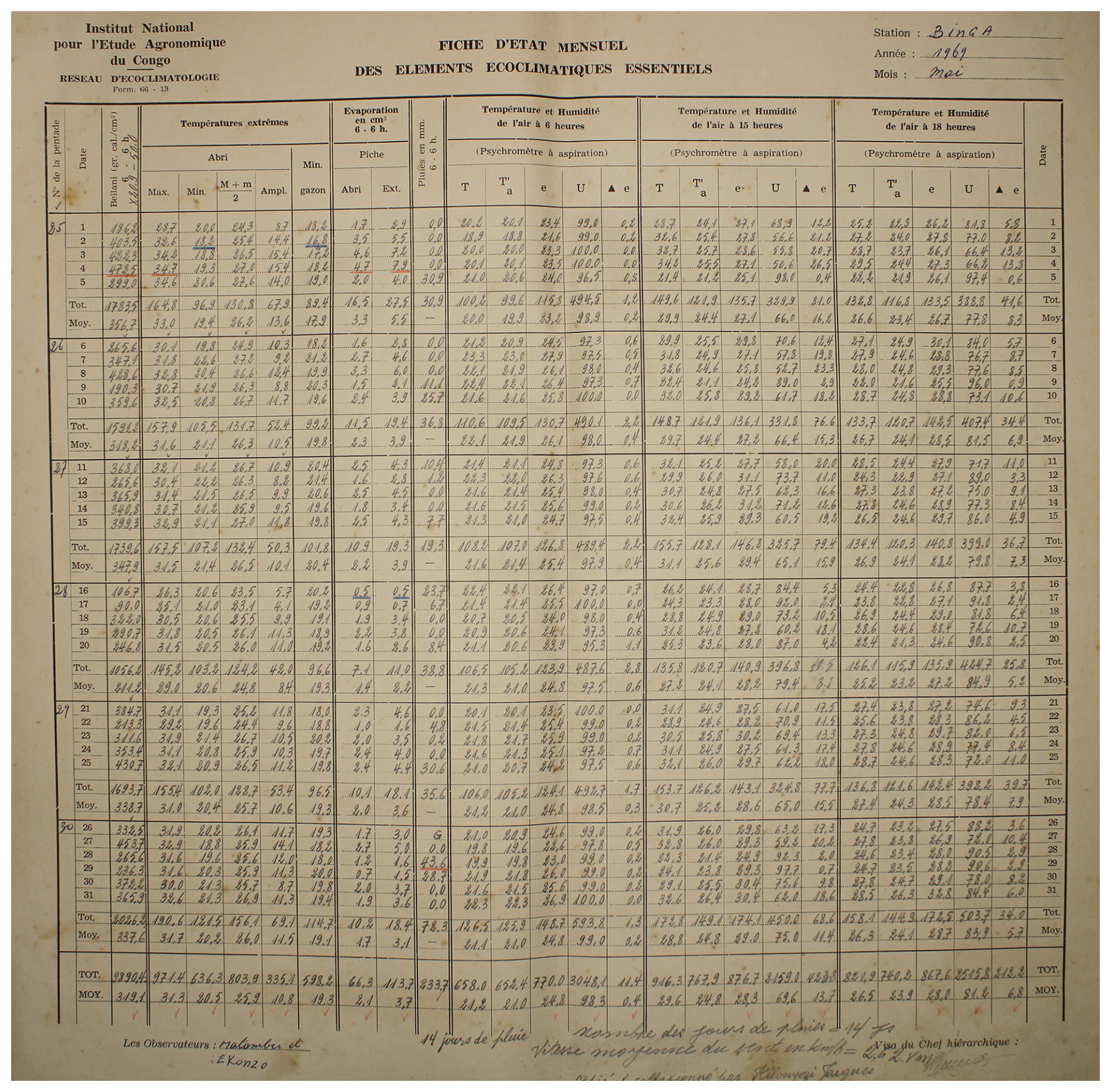
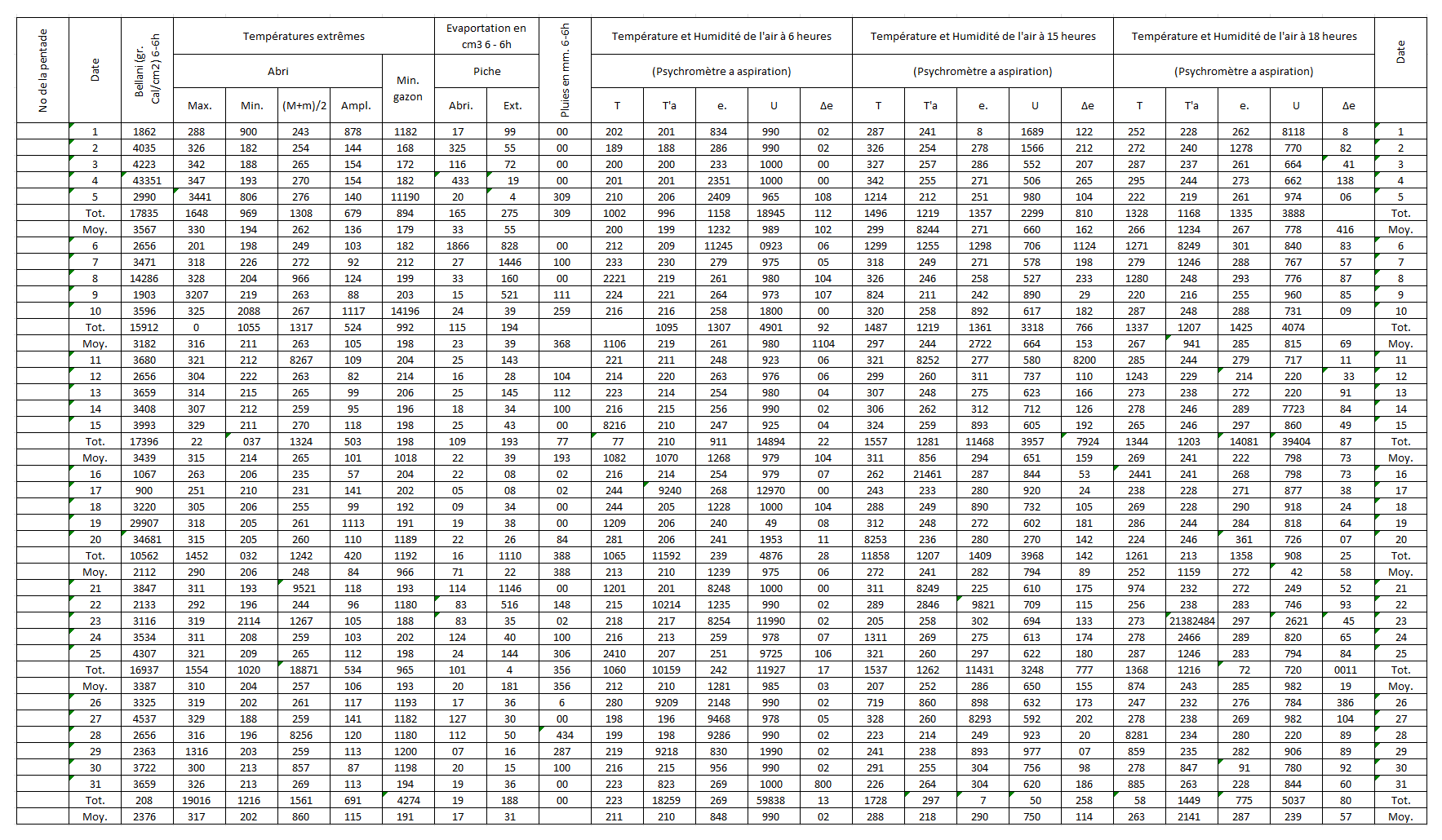
Figure 1 An example one month observed weather data sheet for Station Binga (2°18^′ N, 20°30^′ E) in DRC available within the archives of INERA, Yangambi. The sheet contains the following information: (1) the station name, year (Année) and month (Mois) in the top right corner, (2) the data owner (Institute) in the top left corner, (3) a table (center) showing the pentad number (N^o de la pentade), Date, Bellani (measure for total solar radiation), extreme temperatures in degree Celsius (Températures extrêmes) consisting of maximum, minimum and average temperatures, as well as the diurnal temperature range (Ampl.), Evaporation in centimeter cubed, Rainfall (Pluies) in millimeters per day, and Temperature and Humidity (Température et Humidité) recorded at three times of the day, namely 6 $\mathrm{a}.\mathrm{m}.$, 3 and 6 $\mathrm{p}.\mathrm{m}.$, and (4) observer's names (les observateurs) in the bottom left, authorization signature (Visa du Chef hiérarchique) in the bottom right, and extra comments written in the bottom center of the sheet. Additionally, the table also shows 5 d (and/or 6 d) totals (Tot.) and means (Moy.), as well as monthly totals and mean values. Note that the values in these sheets are all handwritten, and the handwriting styles vary throughout the dataset.

2 Data

To illustrate and test MeteoSaver, we use ten different sheets of meteorological observations across DRC, including daily records of temperature, precipitation, humidity, and other variables. (see Figs. 1, A1–A9, and Table 2). The ten sheets were selected to span a range of handwriting styles, locations, paper size, quality, color, and maintenance conditions. Each sheet records a range of variables at daily resolution across one month, their multi-day totals and averages (5 and/or 6 d), as well as monthly totals and averages. Some variables are directly observed, while others are calculated diagnostics. From the available variables, we here focus on daily minimum temperature (observed), daily maximum temperature (observed), daily mean temperature (diagnosed), and diurnal temperature range (diagnosed) (see Sect. 3.5). The sheets originate from the Yangambi branch of the Institut National pour l'Etude et la Recherche Agronomiques (INERA); a detailed description of the data digitization procedure is provided in Muheki et al. (2026b). All ten sheets were manually transcribed by the main author for use in the independent evaluation (see Sect. 4).

3 MeteoSaver v1.0 software

We have developed an open source software, MeteoSaver, which uses machine learning algorithms to transcribe tabular handwritten historical weather data into spreadsheets ready for analysis (https://github.com/VUB-HYDR/MeteoSaver/, last access: 20 March 2026). The software is written in Python 3.9 and is flexible to be applicable to similar case studies. Here, we describe the setup of MeteoSaver v1.0, which is organized into six modules: (i) configuration, (ii) image pre-processing, (iii) table and cell detection, (iv) transcription, (v) quality assessment and quality control, and (vi) data formatting and upload (Fig. 2). For demonstration purposes, we present the results of each step using one sample data sheet (shown in Fig. 1), and discuss how these steps in MeteoSaver can be applied in similar case studies.

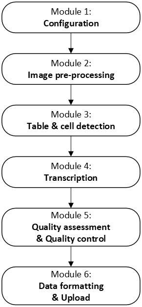
Figure 2 Schematic representation of the modules in MeteoSaver v1.0, illustrating the sequential transcription process from images of paper records to the final digital time series.

3.1 Module 1: configuration

To execute MeteoSaver, the configuration module first requires user settings to ensure smooth operation across different systems, infrastructures, images, and tabular formats (see Table 1). The primary setting, listed under General in Table 1, specifies whether the software will be run on a local machine or HPC infrastructure. On a local machine, the software processes tasks from Modules 2–6 sequentially (see Fig. 2), handling one digitized sheet (and station) at a time. In contrast, when using HPC infrastructure, the software takes advantage of increased processing power, utilizing multiple CPUs and larger dedicated memory, to perform these tasks in parallel for each station. In this case, users can also specify the number of CPUs to be utilized.

Table 1 Configuration: User settings required for execution of MeteoSaver v1.0.

Note: (i) The default settings and values in our case study are described in the subsequent sections (see Sects. 3.3–3.6). (ii) Paths with “…” indicate truncated directory names that are relative to the repository root; see the repository for full names.

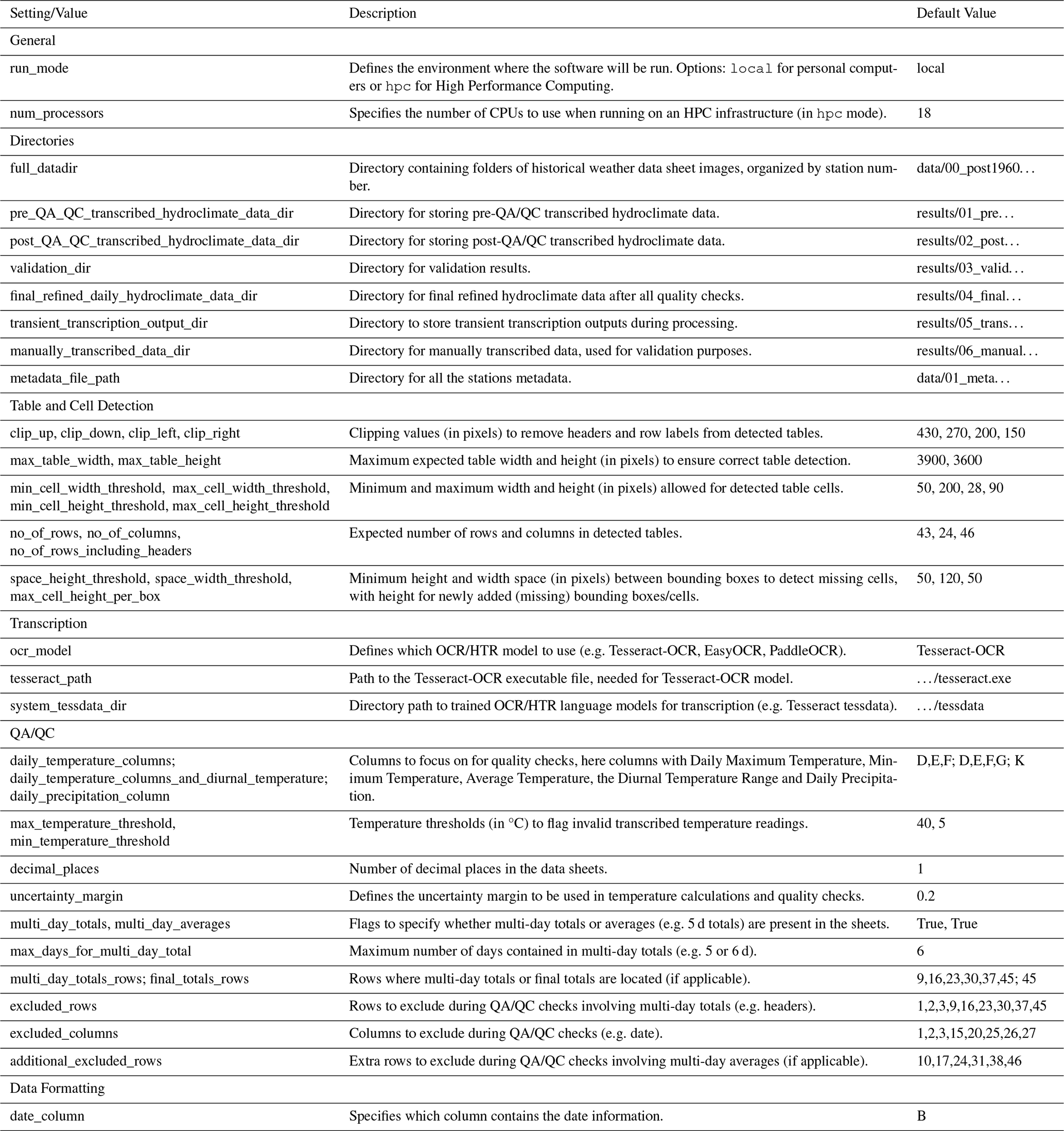
The second step requires specifying the directories for both input and output files, as outlined in Directories in Table 1. For inputs, this includes the folders containing digitized (scanned) historical weather data sheets. For outputs, the locations for the following must be defined: (i) pre-quality assessment and quality control (QA/QC) transcribed data, (ii) post-QA/QC transcribed data, (iii) final refined data, (iv) transient transcription outputs, and (v) manually transcribed data.

Next, the user must input the required settings for the subsequent subsections (Modules 3–6). For Module 3 (Table and Cell Detection), this includes thresholds for maximum table width and height (in pixels) to ensure accurate automatic table detection, as well as clipping values (in pixels) to address table headers and row labels. For Module 4 (Transcription), settings involve selecting the preferred OCR/HTR model, specifying the OCR/HTR execution file directories if applicable, and defining the expected number of rows, columns, and cell dimensions (in pixels) to ensure proper data placement in spreadsheets after transcription. For Module 5 (QA/QC), users configure quality control checks (see Sect. 3.5), including specifying the variables of interest (e.g. daily maximum temperature) and their respective columns, setting thresholds for these variables, defining uncertainty margins, and indicating the presence of multi-day totals or averages, along with their corresponding rows if applicable. Finally, in Module 6 (Data Formatting and Upload), the date column in each sheet is specified as a prerequisite for final data formatting.

These configuration settings ensure the software remains flexible and adaptable to similar case studies. The default settings and values for our case study are described in the following subsections (Sects. 3.3–3.6).

3.2 Module 2: image pre-processing

Within our framework, we use the image processing module of OpenCV (Open Source Computer Vision; http://opencv.org/, last access: 20 March 2026) for pre-processing the images (digitized data sheets). This module, part of the larger OpenCV library, offers multiple computer vision algorithms tailored for image processing. The first step involves loading the images, which should be in an OpenCV-supported format such as JPEG/JPG, PNG, TIFF, BMP, or WEBP. Each image corresponds to data from a single station and month. In our framework, these images follow a specific naming convention: “STN_YYYYMM_SF” or “STN_YYYYMM_HD”, based on the data inventory. Here, STN refers to the three-digit station number, YYYY is the year, MM is the month, SF represents Standard Format (printed tabular format), and HD indicates a hand-drawn version of the standard format. In the following steps, we focus on the images in SF format.

The software processes one image (sheet) at a time on a local machine, or multiple sheets (one per station per allocated CPU) when running on HPC infrastructure. Each image is loaded and converted to grayscale to enhance intensity variations, which is critical for more accurate and efficient table and cell detection (see Sect. 3.3).

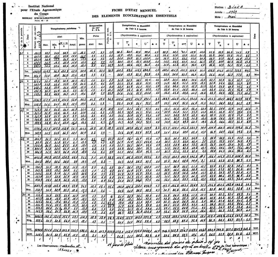
Figure 3 Binary image using adaptive thresholding for an example one month observed weather data sheet for Station Binga (2°18^′ N, 20°30^′ E) in DRC available from the archives of INERA, Yangambi.

Additionally, we binarize the grayscale images using adaptive thresholding, which converts each pixel into either 0 or 1 based on localized thresholds (intensities). Instead of a global threshold, each pixel's threshold is calculated as the mean intensity from a small neighboring area. This method is particularly advantageous for handling images with uneven lighting and localized features, making it ideal for binarizing images with varying paper quality across the sheet and small or faint handwritten text (Yang et al., 1994; Sauvola and Pietikäinen, 2000). Pixels with intensities above the threshold are set to white (e.g. the blank areas on the sheets), while those below the threshold (e.g. the handwritten values) are set to black. The result is a binary image composed entirely of black and white pixels (see Fig. 3), which is optimal for text recognition tasks (as in Sect. 3.4).

3.3 Module 3: table and cell detection

Similarly, we utilize OpenCV's image processing module for both table and cell detection in the pre-processed images (see Sect. 3.2). Here, we employ these ML algorithms following methodologies similar to those described by Badami (2023), customizing them for our case study. First, we binarize the grayscale images again using Otsu's thresholding, which is effective for table detection as it determines a global threshold that maximizes contrast between the foreground and background (Bangare et al., 2015). Unlike adaptive thresholding, which uses localized thresholds, Otsu's method converts the image into pixels of 0 or 1 based on a single automatically calculated threshold (Bangare et al., 2015). This second binary image is used solely for the table detection step in this module.

Next, the table in this second binary image is detected using contours. As described by Yuan et al. (2020), contours are here defined as curves that connect all continuous points with the same color and intensity. Thus, these contours are present for both the individual cells and the entire table in the image (Yuan et al., 2020; Nidhi et al., 2021). In the MeteoSaver framework, we apply morphological operations such as dilation and erosion in OpenCV to close small gaps within the binary image (e.g. gaps in horizontal and vertical lines in the table). This allows us to identify the largest contour in the image as the table. To ensure accurate detection, we set the maximum allowable contour dimensions – table width and height – in the configuration module (see Table 1) to 3900 and 3600 pixels, respectively. This precaution helps avoid instances where the entire sheet is mistakenly identified as the largest contour instead of the table. Using the coordinates of the detected table, we then crop the first binary image (from adaptive thresholding) to isolate the table for further steps (Fig. 4). An additional, but optional, step in our pipeline allows clipping out the headers and the columns with the dates and pentad numbers, allowing us to focus only on the recorded observations (handwritten values). This step is crucial because, in the subsequent Transcription module (Sect. 3.4), we restrict the OCR/HTR model to recognize only digits (0–9). This restriction helps reduce noise from extraneous characters, such as those in the headers and some row labels, thereby enhancing the model's recognition accuracy. In the current version of the software, the latter functionality is tailored to the formats of the ten illustrative sheets considered here, but it can be modified through the configuration module (see Table 1). Moreover, our framework includes a de-skewing function to correct any skew in the table, if present. The function first detects horizontal lines in the image using morphological operations and calculates the average angle of these lines. It then rotates the image by the calculated angle to properly align the horizontal content. This ensures the table is horizontally aligned, a critical step for further analysis.

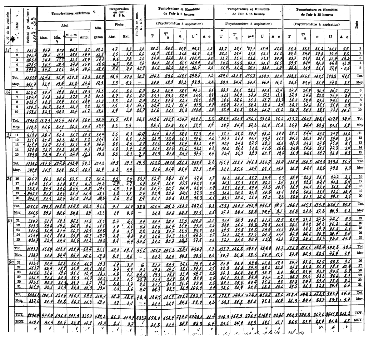
Figure 4 Detected table extracted using MeteoSaver for an example one month observed weather data sheet for Station Binga (2°18^′ N, 20°30^′ E) in DRC available from the archives of INERA, Yangambi.

We then invert the clipped binary image, turning the handwritten values (previously black) to white and the background (previously white) to black. Using OpenCV's structuring element, eroding and dilating features, we identify and erase the vertical and horizontal lines in the inverted images (Yuan et al., 2020) (see Fig. 5). The structuring element allows us to define the pixel neighborhood over which erosion and dilation are applied successively in both the vertical and horizontal directions (Yuan et al., 2020). Erosion shrinks the white regions in the inverted image (including both lines and text), thinning the lines until they disappear, while dilation restores the eroded text by expanding the remaining white regions. The combined effect of these operations produces an inverted image without any horizontal or vertical lines (see Fig. 5). This step is essential for detecting the cells in the table.

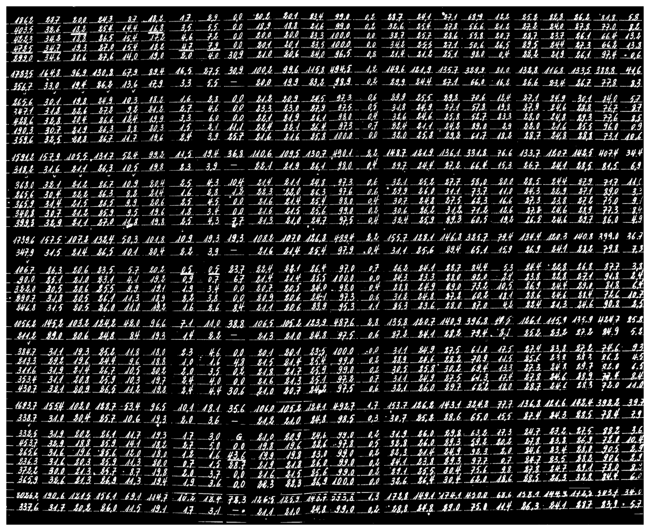
Figure 5 Inverted binary image showing the clipped detected table using MeteoSaver for an example one month observed weather data sheet. Here, we clip the detected table to exclude the headers and row labels such that only the handwritten records are considered for subsequent text detection and transcription steps. In this image, we show how we eliminate both the vertical and horizontal lines from the image using openCV to facilitate the detection of only values as the white blobs in close proximity in the inverted binary image (see Fig. 6).

By applying dilution again on the inverted image without horizontal or vertical lines (as in Fig. 5), we convert the recorded values (text) into white blobs against a black background (see Fig. 6). Contours are then identified around these blobs, enabling the determination of bounding boxes (identified cells) for each detected text area. To filter out small or over sized blobs – often markings or spots on the sheet rather than actual text – we set minimum bounding box dimensions of 50 pixels in width and 28 pixels in height, and maximum dimensions of 200 pixels in width and 90 pixels in height within the configuration module.

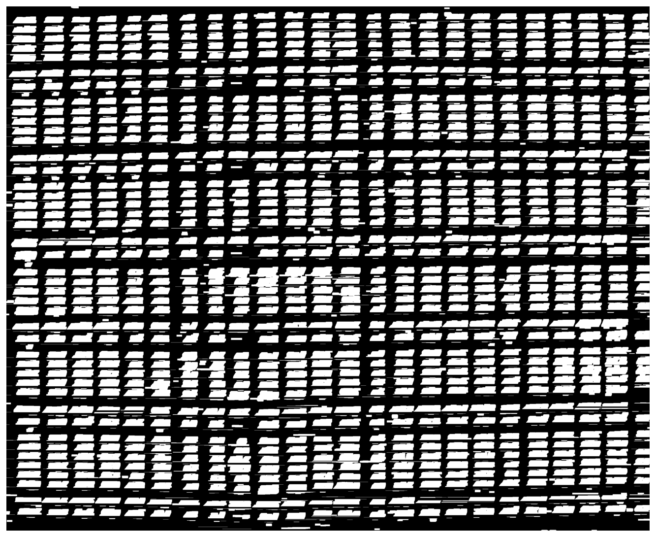
Figure 6 Inverted binary image showing detected text/cell using white blobs in close proximity, in the inverted binary image. The location of these white blobs (detected text) is then used in MeteoSaver to draw boundary boxes on the binary image (see Fig. 7), serving as a prerequisite step for text recognition, here termed as transcription.

An additional, optional step in our framework is to verify the total number of detected bounding boxes per column and insert missing boxes where needed (see Category: Table and Cell Detection in Table 1). Based on the expected number of rows per column (in our case, 43), we identify columns with fewer detected boxes and then check for spaces that exceed the space height threshold (set to 50 pixels) in between bounding boxes. Missing bounding boxes (with a set height 50 pixels) are then inserted into the largest spaces, provided there are neighboring boxes within the same row and that the space between them does not exceed the width threshold (set to 120 pixels), ensuring alignment.

Finally, we overlay all the bounding boxes onto the previously clipped binary images (Fig. 7). These bounding boxes highlight the detected text and table cells in each image. Their dimensions and coordinates are then passed to the Transcription module for further clipping of the table in preparation for the next handwritten text recognition step (Sect. 3.4).

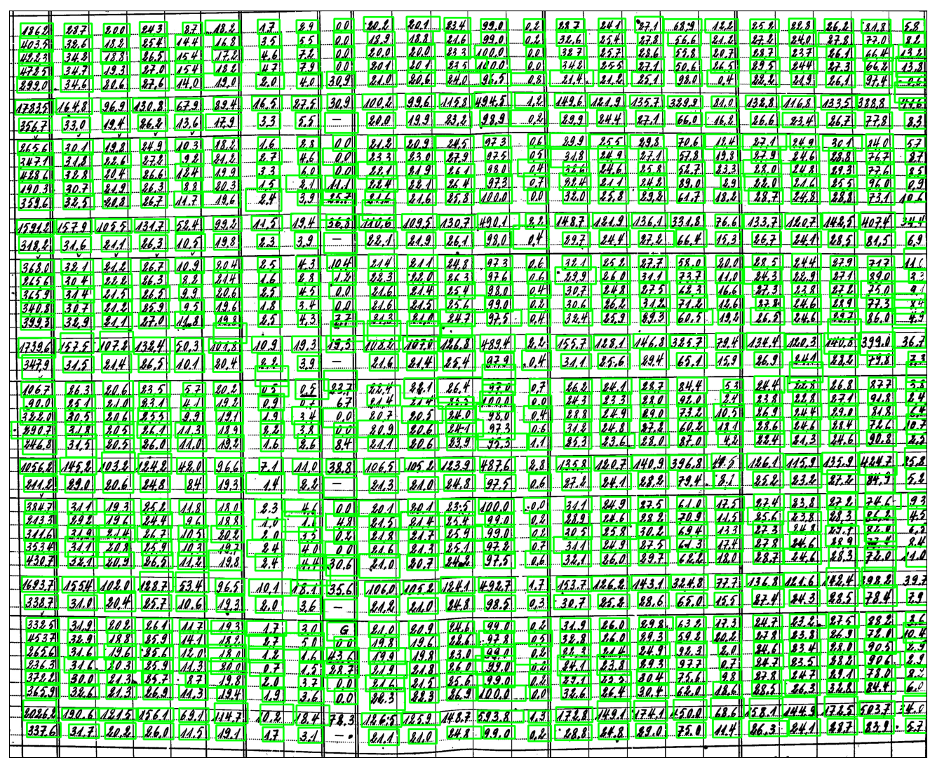
Figure 7 Detected text on the image is highlighted with green boundary boxes. These boxes are then used to clip the image, and the clips are processed by the OCR model to recognize the handwritten values. The coordinates of the boundary boxes are utilized to determine the location of the recognized text for accurate placement in a two-dimensional array.

3.4 Module 4: transcription

The transcription module of MeteoSaver v1.0 leverages our prior work on training an open-source Optical Character Recognition/Handwritten Text Recognition (OCR/HTR) model using the Tesseract OCR framework (Vercruysse et al., 2025). In this prior work, we evaluated both open-source OCR/HTR models, such as Tesseract OCR and Pylaia, and commercial alternatives, including Transkribus, Microsoft Azure, Google Document AI, and Amazon Textract. As demonstrated in Vercruysse et al. (2025), although commercial OCR/HTR models currently offer higher accuracy in text recognition, their use would be extremely costly for transcribing extensive archival datasets and would not align with Open Science principles. For these reasons, we trained the Tesseract OCR model further, enhancing the open-source French Tesseract model with over 35 000 text images from the INERA digitized data (Vercruysse et al., 2025). This was due to the lack of available pre-trained models for handwritten digits in Tesseract OCR, which are primarily optimized for printed text, necessitating additional training. Additionally, following the recommendations in Vercruysse et al. (2025), we provide the option to integrate multiple OCR models within our framework. Currently, MeteoSaver includes two additional open-source OCR models: PaddleOCR (PaddleOCR, 2024) and EasyOCR (JaidedAI, 2023).

In this module, we input clipped binary images, iterating over the detected cells from the previous Table and Cell detection module (bounding boxes shown with green borders in Fig. 7) and feed each into the OCR/HTR model to recognize the handwritten values. To reduce noise from extraneous characters – such as dotted lines in the tables that might be interpreted as decimal points – and to improve accuracy, we restrict the OCR/HTR model to recognize only the digits 0–9.

The bounding box locations are used to identify boxes within the same row using K-means clustering (as in Suresh et al., 2010), while the image width (clipped binary table shown in Fig. 7) determines column placement. K-means clustering groups boxes with similar vertical positions by taking the maximum expected rows as the number of clusters and calculating the average location of each cluster to group boxes into rows. Once row placement is established, column placement is determined by dividing the image into fixed-width segments based on its width, mapping each bounding box to a column using its x coordinate. Finally, we place the recognized handwritten values from each bounding box into a two-dimensional array, organizing them into the correct rows and columns to preserve the original structure of the data. As an additional step, we also define and include the original headers and row labels (such as the Date, Tot. and Moy. labels) in the array (see Fig. 8).

Figure 8 Pre-quality controlled table with transcribed values using MeteoSaver.

3.5 Module 5: quality assessment and quality control

Following the transcription of the data, quality assessment and quality control (QA/QC) is carried out to ensure the final output data is highly accurate with reference to the original handwritten daily temperature records (see Fig. 9). Here, accuracy refers to the agreement between the automatically transcribed and QA/QC confirmed values and their corresponding manually transcribed values, evaluated within a set uncertainty margin to account for small numerical differences arising from rounding or other minor discrepancies. This assumes that the manually transcribed values are correct, which may not always be the case, as manual transcription is also subject to errors depending on the methods applied. This assumption means that the resulting inferred error rates are a conservative estimate.

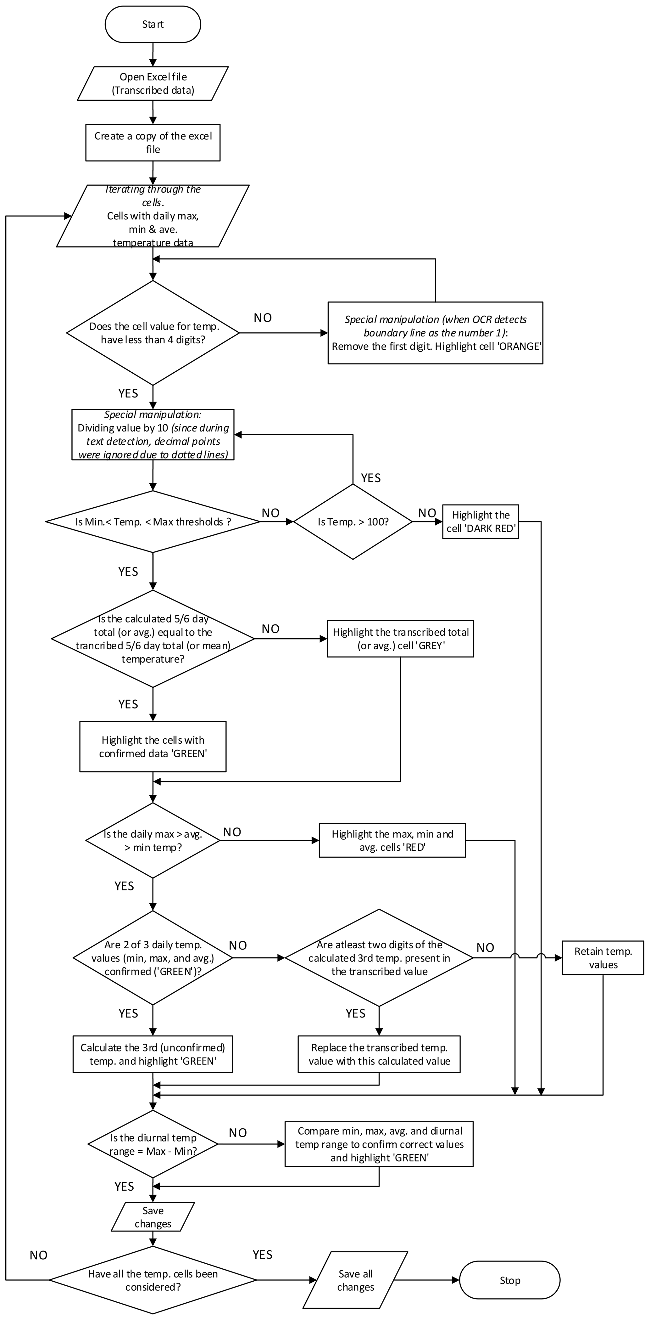
Figure 9 Flow chart showing the quality assessment and quality control checks for the transcribed values with focus mainly on the daily temperature values.

This module performs two complementary roles: (i) validation checks that assess whether the transcribed values are logically and physically consistent, and (ii) correction operations that adjust specific transcription errors where the correct value can be inferred from the structure of the table such as totals or averages, or from related variables.

As a prerequisite, we define the number of decimal places in the original sheets within the QA/QC category of the configuration file (Table. 1, set to one decimal place in our case. This is because during the transcription, the OCR/HTR model is restricted to recognize only digits 0–9 (see Sect. 3.4). We also define the specific columns to assess, in our case those containing daily maximum, minimum, and average temperatures (T_max, T_min, and T_avg, respectively), along with the diurnal temperature range (DTR). Another key user setting addresses the presence of multi-day totals or averages within the sheet, such as pentad (5 and 3, 4, or 6 d for the final pentad, depending on the month), weekly, 10 d, or monthly sums and means. In our case study, the sheets include pentad totals and averages (Figs. 1 and 8).

Additional user settings in the QA/QC category of the configuration module include: (i) specifying an uncertainty margin (in degrees Celsius) for recorded temperature values to account for potential rounding errors during observations, particularly in average temperature readings. In our case, this margin is set to 0.2 °C, meaning QA/QC checks will only flag transcribed values for correction if they fall outside this range when compared to calculated temperatures obtained during QA/QC. (ii) defining maximum and minimum temperature thresholds to identify unusually high or low values that may have been erroneously transcribed, with reference to regional temperature ranges from the literature. According to Alsdorf et al. (2016), the average daily maximum temperatures reported within the Congo basin during the period 1950–1959 were between 30–31 °C, with an approximate increase in daily temperatures of 0.60–1.62 °C per 30 year period. Therefore, we use 40 °C as the threshold for daily maximum temperature in the illustrative case study to ensure extremes are captured, but transcription errors are identified. For the daily minimum temperature threshold, we use 5 °C. Following this, a series of QA/QC checks are conducted on the transcribed data by loading the two-dimensional array from the Transcription module into a spreadsheet format and creating a backup copy of the file (see Fig. 9). Only daily temperature values that pass the following QA/QC checks are included in the final time series for their respective stations (see Figs. 13–14).

The first check involves verifying that the transcribed values for T_max, T_min, and T_avg contain fewer than four digits. This check is specific to daily temperature values recorded in °C units with one decimal place, where the decimal place is deliberately not recognized by the OCR/HTR model. For example, a value of 27.8 °C would be correctly transcribed as “278” (Fig. 11a and b). Therefore, if more than three digits are detected (e.g. MeteoSaver reads “1278”), it is likely that a wrong transcription was made. If this condition is not met, a specific adjustment – unique to our sheets – is applied: the first digit is removed from the value (i.e. “1278” becomes “278” in our example through this data transformation step), and the cell is flagged to indicate this manipulation (see Fig. 11a and b, with manipulated values in b shown in orange). This adjustment addresses cases where the OCR/HTR system mistakenly interprets a cell boundary line as an extra digit, such as “1” (as in Fig. 11a and b). This data transformation assumes that the first digit of the wrongly transcribed value is erroneous which may not always be true, for example, if an extra digit occurs in the middle or at the end of the value.

However, if the check is passed, the transcribed temperature values are then adjusted to match the required decimal places, set to one in this case (see Fig. 11b and c, “278” becomes “27.8” in our example through this postprocessing step). This step corresponds to a scaling operation based on the number of decimal places specified in the configuration settings (Table. 1). This is because the original observations were recorded to one decimal place (Figs. 1, A1–A9), whereas the OCR/HTR model was restricted to recognize only digits (0–9) to avoid misinterpreting dotted table lines as decimal points.

In the second check, daily temperature values are tested to ensure they fall within the set maximum and minimum thresholds and are flagged if they do not (see Fig. 11c and d, with flagged values in d shown in dark red). If a daily temperature value exceeds the maximum threshold and is also greater than 100, a specific adjustment is applied by dividing the value by 10. For values within the thresholds, the multi-day (here, pentad) totals and averages for T_max, T_min, and T_avg are calculated and compared with the transcribed multi-day totals and averages. Similarly, the multi-day totals for daily precipitation values (P) are calculated and compared with the transcribed multi-day totals. If the transcribed values match (or are within the set uncertainty margin of) the calculated totals or averages, both the multi-day values and their respective daily values are flagged as confirmed or not confirmed accordingly (see Fig. 11c and d, with unconfirmed pentad total and average values in d shown in grey).

Thereafter, logical checks are performed for each day (that is to say, per row) as follows: (i) T_min must be less than T_avg, which in turn must be less than T_max, with values flagged if this condition is not met. (see Fig. 11h, with flagged values in red). (ii) if two of the three daily temperature values (T_max, T_min, and T_avg) have already been confirmed through previous checks, the third unconfirmed value would then be calculated (using Eq. 1) and flagged as confirmed. (iii) If the above condition is not met, but at least two digits of the calculated third value match those in the transcribed third value, we replace the transcribed value with the calculated one and flag the three values as confirmed. (iv) if the transcribed value for T_avg is equal to (or is within the set uncertainty margin of) the average of the transcribed T_max and T_min of that same day (as in Eq. 1), all daily values are confirmed (see Fig. 11d and h, with confirmed T_max, T_min, and T_avg in h shown in green. (v) the relationship between T_max, T_min, and T_avg, and the transcribed diurnal temperature range (DTR) is then used to correct unconfirmed values. Here, we iterate through three equations (Eqs. 2–4) to calculate the unconfirmed transcribed values for T_max, T_min, and T_avg, and to confirm those transcribed values that fall within the set uncertainty margin (see Fig. 11g and h, with confirmed T_max, T_min, T_avg and DTR in g shown in green). The following equations define the relationships between T_max, T_min, T_avg, and DTR:

First, the daily average temperature is calculated as:

$$\begin{array}{}\text{(1)}& {\displaystyle }{\displaystyle }{T}_{\text{avg}}={\displaystyle \frac{T_{\text{max}}+T_{\text{min}}}{\mathrm{2}}}\end{array}$$

Next, the diurnal temperature range (DTR) is defined as the difference between T_max and T_min:

$$\begin{array}{}\text{(2)}& {\displaystyle }{\displaystyle }\text{DTR}=T_{\text{max}}-T_{\text{min}}.\end{array}$$

Figure 10 Key for the colors (flags) showing quality assessment and quality control checks shown in Figs. 11 and 12.

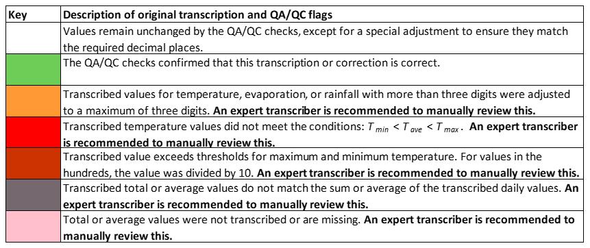
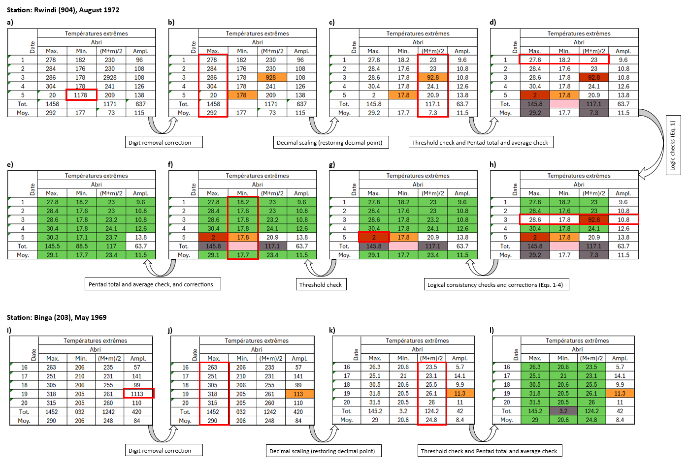
Figure 11 Two examples of pentad transcribed temperature values (Top: Station Rwindi [0°47^′ S, 29°17^′ E], August 1972, and Bottom: Station Binga [2°18^′ N, 20°30^′ E], May 1969) illustrate the sequence of QA/QC checks performed on the initial transcribed values, leading to the final confirmed values (flagged in green). The arrows, along with their respective labels between each panel, indicate the specific QA/QC checks applied at each stage for the pentad, corresponding to the procedures and equations described in Sect. 3.5 and illustrating the progression of the QA/QC workflow. Red-bordered cells, rows, or columns highlight examples where unconfirmed transcribed values were identified and corrected during QA/QC, with changes reflected in the subsequent panel. See Key for all colors (quality flags) in Fig. 10.

Then, by substituting terms from Eq. (1), DTR can also be expressed in terms of T_avg and T_min (in cases of unconfirmed or incorrectly transcribed T_max values) as:

$$\begin{array}{}\text{(3)}& {\displaystyle }{\displaystyle }\text{DTR}=\mathrm{2}{T}_{\text{avg}}-\mathrm{2}{T}_{\text{min}}.\end{array}$$

Or in terms of T_max and T_avg (in cases of unconfirmed or incorrectly transcribed T_min values) as:

$$\begin{array}{}\text{(4)}& {\displaystyle }{\displaystyle }\text{DTR}=\mathrm{2}{T}_{\text{max}}-\mathrm{2}{T}_{\text{avg}}.\end{array}$$

Lastly, temperature threshold checks, as well as multi-day temperature totals and averages, are re-assessed as previously described to leverage all confirmed temperature values for correcting any remaining unconfirmed T_max, T_min, and T_avg values (see Fig. 11f and g and Fig. 11e and f, respectively, with confirmed T_max, T_min, and T_avg values shown in green). We follow the sequence of QA/QC checks outlined above, starting with vertical checks (columns) and then moving to horizontal ones (rows). This approach first confirms values with more inputs (in this case, columns with 5 or 6 values using the total or average), followed by values with fewer inputs (rows with 3 or 4 values). This order minimizes the risk of incorrectly confirming values based on limited input data.

Each of the checks described above assigns a quality flag to the data, color-coded according to Fig. 10 as follows: (i) White cells indicate values that remain unchanged from the original transcription, except for adjustments to match the required decimal places (here, 1 decimal place). (ii) Green cells represent values confirmed as correct by the QA/QC checks, either as transcribed or calculated. (iii) Orange-highlighted cells indicate that the original transcribed temperature value had more than three digits and was adjusted to three digits. (iv) Red cells highlight cases where transcribed temperature values did not meet the conditions $T_{\text{min}}<T_{\text{avg}}<T_{\text{max}}$. (v) Dark red cells show that the transcribed value exceeded the set thresholds for maximum or minimum temperature. (vi) Grey cells indicate that the multi-day (here, 5 d) total or average did not match the sum or average of the transcribed daily values. (vii) Finally, pink cells indicate missing or untranscribed multi-day total or average values. Only the confirmed (green) daily temperature values are passed to the next module, Data Formatting and Upload (Sect. 3.6). It is recommended that values flagged in white, orange, red, dark red, grey, and pink be manually reviewed by an expert transcriber.

In addition to the checks described above, an optional time series consistency check can be applied once a longer temperature series is available for a given station. This step requires the consolidation of daily observations across multiple sheets and therefore cannot be applied during the initial QA/QC stage. It involves identifying outliers in the temperature time series for each station by using standard deviation to detect unusual patterns in the transcribed temperature records (as in Chauhan and Parashar, 2020). This check within our framework unfolds in two steps, following the creation of a distribution of all values across the station's time series: (i) Temperature values that deviate more than three standard deviations from the mean are identified, flagged, and removed (until confirmed by an expert). (ii) we identify abrupt transitions in daily temperature by examining the standard deviation differences of consecutive days. Specifically, we check for cases where a large deviation (e.g. less than −4 standard deviations from the mean) on one day is followed by a large deviation in the opposite direction (e.g. more than +4 standard deviations) on the next day, and then a return to a similar deviation on the third day. When this pattern is observed, we flag the middle day as an outlier and remove it from the time series (until confirmed by an expert). For example, if a sequence of days shows a temperature that deviates significantly below the mean, followed by a sharp increase above the mean, and then returns to a lower deviation on the following day, the middle day is flagged. This approach allows us to capture rapid shifts in temperature that may indicate transcription errors or anomalies, even if the individual values do not exceed the fixed ±3 standard deviation threshold used in the first method. Although included in our framework, the first step is not applied in this demonstration because we illustrate with a single month's data (a short series), where it could lead to mistakenly removing extreme but valid values.

3.6 Module 6: data formatting and upload

In the final module of MeteoSaver, we consolidate all confirmed daily transcribed data (flagged in green) from the previous QA/QC module across all monthly sheets for each station to create long temperature time series per station. As a prerequisite, users specify the column in the monthly sheets that contains date information in the configuration file (see Sect. 3.1). Additionally, the month and year information for each monthly sheet is automatically retrieved from the file names, following the naming convention outlined earlier (see Sect. 3.2).

Finally, we prepare the confirmed historical weather data time series (in this case, temperature) for upload to open-access repositories. In our framework, we convert the data into the standard format prescribed by the Copernicus Data Rescue Service, known as the Station Exchange Format (SEF) (https://datarescue.climate.copernicus.eu/station-exchange-format-sef, last access: 17 April 2026). This format standardizes digitized historical weather records, ensuring compatibility with the Copernicus observational database, facilitating integration and access for climate research and data applications. We integrate the confirmed data with relevant metadata for each station, as specified by the user under the Directories category in the configuration module (see Table 1). This metadata includes key station details such as station name, ID, latitude, longitude, altitude, data source, units, and other relevant information.

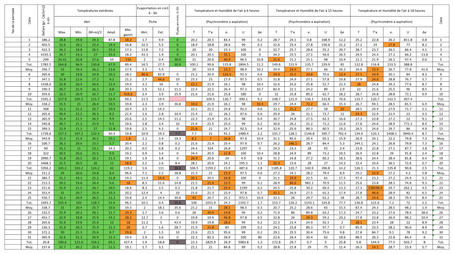
Figure 12 Post-quality controlled table using MeteoSaver, showing confirmed values of daily maximum, minimum and average temperature, diurnal temperature range, and daily precipitation (highlighted in green) for the weather sheet shown in Fig. 1. The description of the colors in the post-quality controlled table is given in Fig. 10.

4 Software evaluation and results

We apply MeteoSaver v1.0 on ten sample data sheets (see Appendix Figs. A1–A9) considering various handwriting styles, paper sizes and formats, and maintenance conditions (ranging from well-preserved in the archives to poor or torn). Here, we present the final results from the QA/QC checks and final data formatting of the transcribed ten sample sheets (Table 2 and Figs. 13 and 14). In addition, we provide the results for all module steps detailed in Sect. 3 (Appendix Figs. B1–B9). We validate the accuracy of MeteoSaver's output in our case study by comparing it to data obtained from manual transcription of these sample data sheets. (Table 2).

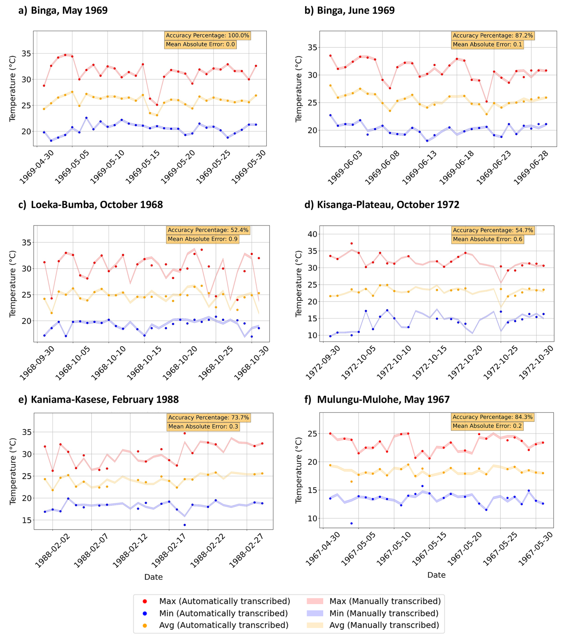
Figure 13 Time series plot of the daily maximum (red), average (orange), and minimum (blue) temperatures for the respective stations. Each variable shows automatically transcribed values as solid markers, while manually transcribed values are displayed as lighter time series bands with a 0.2 °C uncertainty margin applied during QA/QC checks. The accuracy percentage and mean absolute error (MAE) between the automatically and manually transcribed values are noted in the upper right corner of the plot. The accuracy percentage denotes the percentage of confirmed, automatically transcribed values that fall within 0.2 °C of the manually transcribed value. Together, these metrics quantify the agreement between the automatically transcribed values using MeteoSaver v1.0 (markers) and their corresponding manually transcribed values (bands), providing an indication of the reliability of the automatically transcribed observations (with respect to manual transcriptions) for subsequent climatological analyses. The analysis assumes that the manually transcribed values are correct; however, this may not always be the case, as manual transcription is also subject to errors depending on the methods applied.

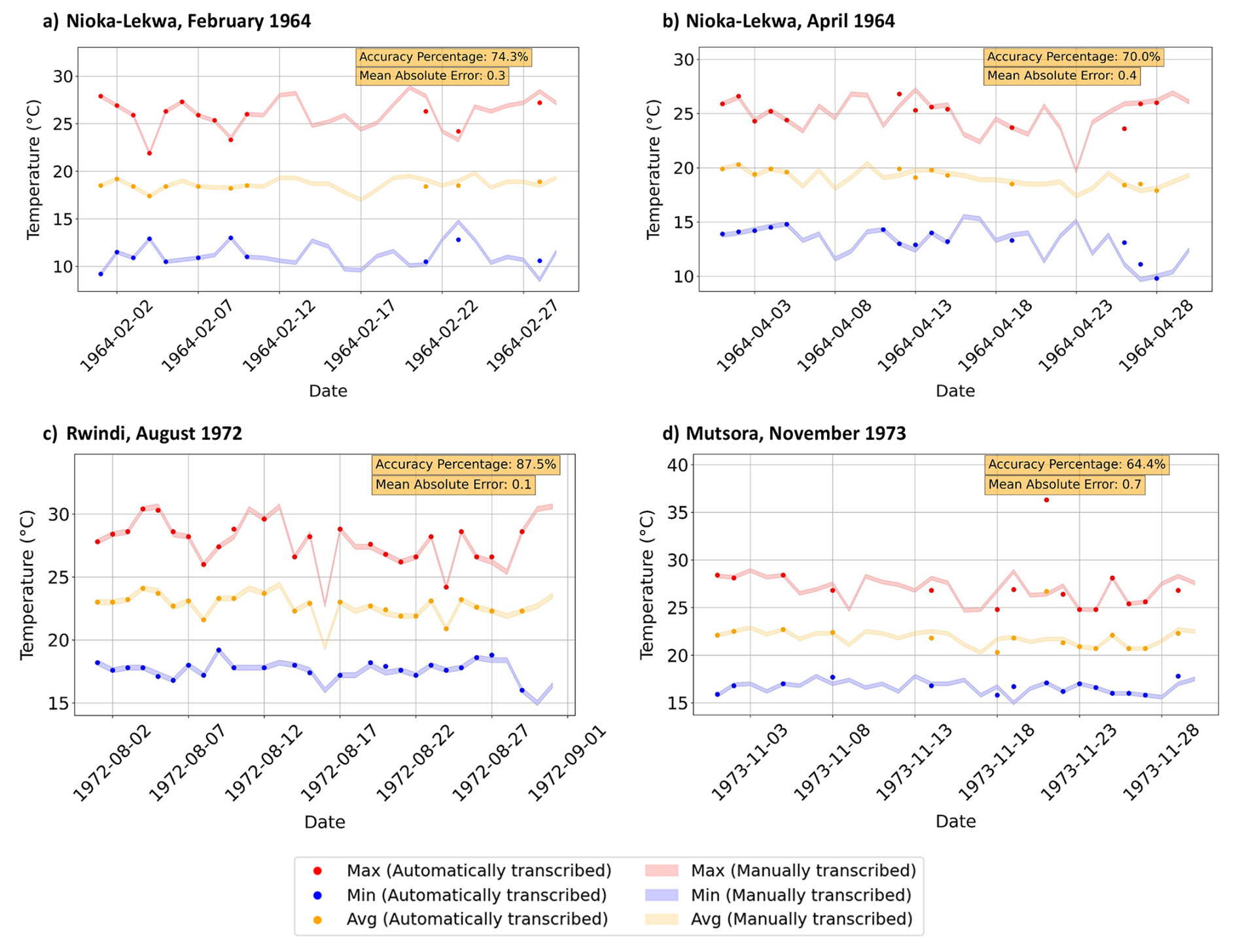
Figure 14 Time series plot of the daily maximum (red), average (orange), and minimum (blue) temperatures for the respective stations. Each variable shows automatically transcribed values as solid markers, while manually transcribed values are displayed as lighter time series bands with a 0.2 °C uncertainty margin applied during QA/QC checks. The accuracy percentage and mean absolute error (MAE) between the automatically and manually transcribed values are noted in the upper right corner of the plot. The accuracy percentage denotes the percentage of confirmed, automatically transcribed values that fall within 0.2 °C of the manually transcribed value. Together, these metrics quantify the agreement between the automatically transcribed values using MeteoSaver v1.0 (markers) and their corresponding manually transcribed values (bands), providing an indication of the reliability of the automatically transcribed observations (with respect to manual transcriptions) for subsequent climatological analyses. The analysis assumes that the manually transcribed values are correct; however, this may not always be the case, as manual transcription is also subject to errors depending on the methods applied.

The results indicate that between 95 %–100 % of the handwritten temperature records (daily maximum, minimum, and average temperatures) from the 10 sheets were successfully detected using the Table and Cell Detection module, with a median of 100 % of cells identified across the sheets. These detected cells were then automatically transcribed by our software. Of these transcribed values, a median of 74.4 % across the sheets achieved the highest quality flag and were therefore confirmed by the QA/QC. This means that 25.6 % of the transcribed values were excluded from the final output timeseries because they could not be confirmed by the QA/QC. The confirmed temperature values showed a median match rate of 74 % with manually transcribed records (see Table 2). Here, accuracy is defined as the proportion of automatically transcribed and QA/QC confirmed values that match manually transcribed values, considering a set uncertainty margin of 0.2 °C. Additionally, we calculate the mean absolute error (MAE) of these automatically transcribed temperature values compared to the manually transcribed ones. The MAE across these transcribed sheets ranged from 0.0–0.9 °C, with a median of 0.3 °C (see Table 2).

Table 2 Validation results of ten sample data sheets transcribed using MeteoSaver v1.0.

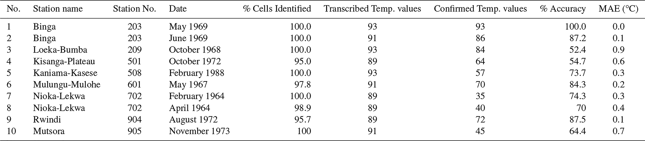
Where: The transcribed values are the daily maximum, minimum, and average temperatures. Accuracy takes into consideration an uncertainty margin of 0.2 °C for transcribed and calculated (confirmed) temperature values.

5 Discussion

In this demonstration, we illustrate the application of MeteoSaver v1.0 on ten sample sheets, where machine learning algorithms are used both to detect tables and cells and to transcribe the data within them. The software also performs QA/QC checks to flag confirmed values and formats the data into Station Exchange Format (SEF) for upload to open-access repositories. The ten sheets, with various handwriting styles, paper sizes, and maintenance conditions, are used to evaluate its flexibility and accuracy in transcribing historical weather data.

Processing each sheet on a local machine equipped with an 11th Gen Intel^® Core™ i7-1165G7 and 16.0 GB of RAM takes under 8 min. Because MeteoSaver processes individual sheets independently, and because it can also be executed on HPC infrastructure through the configuration settings (Sect. 3.1), the transcription process can be parallelized across multiple CPU cores to allow multiple sheets to be processed simultaneously, significantly reducing the total processing time for large archives. For example, processing 1000 sheets sequentially on a local machine would require approximately 130 h, whereas distributing the workload across 20 parallel CPU cores with the same specifications on HPC infrastructure would reduce the processing time to under 7 h. The parallel processing of individual sheets also means that computationally intensive steps such as image pre-processing, table and cell detection and transcription can take advantage of increased processing power and larger dedicated memory on HPC infrastructure.

While the initial transcription results from this sample are promising, with a median accuracy of 74 %, there are limitations in this first version of the software. In the following subsections, we discuss the strengths and weaknesses of this version, highlight developments that were excluded from the initial release, and provide ideas for future improvements in each module.

5.1 Table and cell detection

In our framework, the current table and cell detection module, which utilizes OpenCV's ML algorithms, performs well in identifying tables and cells within entire sheets, achieving a cell detection rate of 95 %–100 % across the sheets (see Table 2). However, while our additional step of adding missing bounding boxes (cells) based on the expected number of rows per column (in our case, 43) generally yields good results, it has some limitations. In some instances, a missing bounding box is added in a large gap between rows that does not actually correspond to a cell (see Fig. 7).

To address this limitation, we explored an alternative approach during software development that involves template matching. In this method, horizontal and vertical guides (lines) are defined for each table layout template using image editing software and overlaid on the sheet to represent cell boundaries. However, this method proved time-consuming, as it requires manually defining guides for each specific template and paper size to ensure accurate alignment with the table lines on different images. This approach therefore becomes impractical for sheets with varying paper sizes or slight modifications in table layout (e.g. the same template but with different row or column widths). Consequently, it lacks re-usability across different case studies, as each user would need to create their own template guides – an unrealistic demand for large historical datasets with diverse templates and paper sizes.

For these reasons, we retained the current table and cell detection module in this initial release. We recommend further refinement within this table and cell detection pipeline to achieve closer to 100 % cell detection accuracy across various table templates.

5.2 Transcription

Within this software release, we offer three open-source OCR/HTR models for text transcription within the identified cells (bounding boxes): Tesseract OCR, EasyOCR, and PaddleOCR. We primarily demonstrate transcription using Tesseract OCR, as it outperforms the other two models due to the availability of our custom-trained language dataset based on the off-the-shelf French Tesseract OCR model, further enhanced with thousands of images of handwritten digits (as detailed in our previous work Vercruysse et al., 2025). While EasyOCR and PaddleOCR are included for flexibility, they are mainly optimized for printed text and digits, making Tesseract the preferred choice for the handwritten data in our sheets. Nevertheless, we include them within our framework for easier integration with potential updates of the models or language datasets, including adaptations for typeset or printed digits.

To minimize noise from extraneous characters, we restrict the OCR/HTR recognized characters within the bounding boxes to digits 0–9. This prevents misreadings, such as dotted lines being read as decimal points or certain handwritten digits being mistakenly recognized as letters. This process generates a two-dimensional array of initially transcribed values, temporarily disregarding decimal places, organized into rows and columns based on bounding box coordinates (see Sect. 3.4 and Fig. 8). The original decimal places, as specified by the user (see Table. 1) are reinstated in the subsequent QA/QC module (as in Fig. 12). For additional characters like minus signs, users are advised to include the minus sign in the OCR/HTR-recognized character set.

5.3 Quality assessment and quality control

The QA/QC results in this release, as outlined in Sect. 3.5, demonstrate that our current pipeline is robust in identifying transcription errors by employing (i) user-defined data thresholds, (ii) multi-day totals and averages, (iii) logic checks, such as $T_{\text{min}}<T_{\text{avg}}<T_{\text{max}}$, (iv) iterative comparisons between related variables, including the relationship between T_min, T_avg, T_max, and the Diurnal Temperature Range (DTR), and (v) reiteration across the different checks (Fig. 9).

It is important to note that some QA/QC checks, specifically the user-defined thresholds (here, maximum and minimum temperature thresholds), are region-specific and should be informed by expert knowledge or prior climatological studies. However, while these regional thresholds are generally effective for identifying incorrectly transcribed values, they may potentially flag correctly transcribed observations associated with extreme events, potentially excluding these undocumented local extremes in the final output dataset.

Notably, the presence of pentad totals and averages in our sheets proved particularly valuable for QA/QC, as they simplified the process of recalculating and confirming transcribed values within each pentad. In contrast, the more common monthly totals and/or averages found in many international archived weather data sheets would present greater challenges, particularly when multiple daily values are transcribed incorrectly.

An evaluation of the values that achieved the highest quality flag revealed a median confirmation rate of 74.4 % of the transcribed temperature data across the sheets, either confirmed or corrected during QA/QC. This means that 25.6 % of the transcribed values were excluded from the final output timeseries. Among these excluded values, a substantial fraction is correctly transcribed but could not be validated by the QA/QC framework. This may occur, for example, when incorrectly transcribed values appear within the same pentad, preventing confirmation of the correctly transcribed values through the QA/QC checks, or in rare cases when extreme but valid observations fall outside the predefined threshold criteria. While the QA/QC checks are used to validate and refine the transcribed data, as demonstrated in Fig. 11, their effectiveness heavily relies on the initial transcription quality, which depends on the OCR/HTR model, the variability in handwriting styles, and the maintenance condition of the paper sheets in the archives. For instance, when the paper condition is well-preserved (as in Fig. 1) and the initial transcription is nearly accurate across most cells, only the first few QA/QC checks are typically sufficient to confirm all daily temperature values in a pentad, as illustrated in Fig. 11i–j. On the other hand, in cases where the initial transcription contains multiple errors, all QA/QC checks and iterative re-evaluations in our framework are necessary to confirm the temperature values in that pentad, as seen in Fig. 11a–h. The latter could, in rare cases, lead to incorrectly confirmed values if the originally transcribed data contains errors that still meet multiple QA/QC checks, or may result in values falling outside the user-defined uncertainty margin, which would therefore remain unconfirmed. Users should be aware that the current QA/QC framework may exclude some valid extreme observations and therefore additional manual verification is advised for applications focusing on rare extremes.

In our study, the final confirmed temperature values showed a match rate of 52.4 %–100 % with manually transcribed records, yielding a median accuracy of 74 % and a median mean absolute error of 0.3 °C (see Table 2). While the accuracy indicates the proportion of automatically transcribed values that match the manually transcribed values with a predefined uncertainty margin, the MAE provides an indication of the magnitude of transcription deviations. The median MAE of 0.3 °C observed in these sample sheets is comparable to typical uncertainties associated with historical thermometer measurements of 0.2 °C (1σ) (Morice et al., 2012; Brohan et al., 2006; Folland et al., 2001). Because many climatological analyses rely on aggregated statistics derived from combined station data, such as spatial averages and long-term trends, transcription deviations of this magnitude are unlikely to substantially affect the resulting climatological interpretations (Brohan et al., 2006). However, for analyses requiring precise daily values such as extreme-event detection, additional manual verification may still be advisable.

These reported performance metrics are specific to this study's sample weather sheet formats, input image quality, handwriting styles on these sheets, paper maintenance conditions, and manual transcription quality. Consequently, the reported performance may differ when MeteoSaver is applied to other historical datasets with different table structures, handwriting styles or image quality. Additionally, the variability of climate variables should be considered, for example, while temperature values in the DRC exhibit relatively small annual ranges, extratropical regions often experience much larger seasonal variations (on the order of tens of degrees). In such contexts, transcription errors may be larger and more difficult to detect through the applied QA/QC procedures. Nevertheless, the modular design of MeteoSaver allows users to adapt the configuration and retrain the OCR/HTR models to accommodate different table layouts and handwriting styles.

To enhance transcription accuracy, we recommend further training of the OCR/HTR model on a wider range of handwriting styles, specifically for handwritten digits. This would improve transcription accuracy even prior to the QA/QC step, subsequently enhancing the accuracy of QA/QC-verified values. Moreover, in future software versions, we suggest incorporating a feedback loop where corrected and confirmed values from the QA/QC process serve as additional training data for the OCR/HTR models. This iterative approach would enable the OCR/HTR model to continuously learn from past corrections and improve its ability to transcribe specific handwriting styles over time. This “on-the-fly” learning capability would progressively increase the model's transcription accuracy with each batch of post-processed data.

While our demonstration focuses exclusively on QA/QC checks for daily temperature and precipitation values, the evaluation of this first version of the software primarily focuses on temperature variables (daily maximum, minimum, and average temperatures). This choice was made because temperature allows the illustration of a broader set of QA/QC procedures available in the sheets, including pentad totals and averages, logical consistency checks (e.g. $T_{\text{min}}<T_{\text{avg}}<T_{\text{max}}$), diurnal temperature range checks, and threshold tests. Together, these checks provide a comprehensive demonstration of the QA/QC framework implemented in MeteoSaver. In contrast, precipitation values presented in the sample sheets include only one QA/QC constraint: the pentad total, which limits the ability to identify and correct erroneously transcribed daily precipitation values. As a result, fewer daily precipitation values can be confirmed through the QA/QC framework compared with daily temperature values (Figs. 12 and B1–B9).

Nevertheless, future software versions could expand these checks to include additional variables and diagnostics. For instance, in our sheets, the columns under Température et Humidité contain vapor pressure (e) and relative humidity (U) recorded at specific times, which are calculated using the observed dry-bulb temperature (T) and wet-bulb temperature ($T_a^{\prime }$). This would allow us to incorporate more equations within the QA/QC module to validate an even broader range of transcribed values across the sheets. Therefore, for this initial release, we provide a detailed description of the current QA/QC checks to guide software users and illustrate the framework's flexibility.

5.4 Potential of the software

Our study demonstrates the flexibility of MeteoSaver in transcribing historical tabular weather data across a range of handwriting styles, table dimensions, paper sizes, and maintenance conditions, highlighting its potential contribution to ongoing climate data rescue efforts. Throughout our model development, we focused on reusability for similar case studies, equipping MeteoSaver with numerous configurable settings within the configuration module (see Sect. 3.1) to allow users to tailor the software for specific table formats. Given this flexibility, MeteoSaver has substantial potential for transcribing millions of rescued archived weather records, such as those available on the C3S Data Rescue Service Portal. It is important to note, however, that in this initial release, users may need to make further adjustments when applying the software to data sheets with complex tabular formats or variables or data types beyond temperature and precipitation, particularly within the QA/QC checks.

MeteoSaver therefore complements existing efforts in historical climate data rescue. Many recent efforts rely on manual transcription workflows, including citizen science initiatives (Noone et al., 2024; Hawkins et al., 2019; Craig and Hawkins, 2020), while other approaches explore open-source and commercial OCR/HTR models to directly transcribe individual values in scanned historical documents (Vercruysse et al., 2025; Nockels et al., 2022). MeteoSaver, on the other hand, contributes to these existing data rescue efforts by providing an open-source end-to-end workflow that integrates machine-learning into image processing, table and cell detection, and transcription, as well as QA/QC and data formatting ready for upload. In addition, MeteoSaver can potentially make use of quality-controlled manually transcribed data as training data with multiple handwriting styles for the OCR models used in the transcription module. By automating these key steps of the data rescue process, following the digitization (imaging) of paper-based records, MeteoSaver aims to substantially reduce the manual effort required for climate data rescue while integrating QA/QC procedures into OCR/HTR-based transcription workflows. Furthermore, its modular and open-source framework allows for continuous improvement of the machine-learning components as additional training data becomes available.

While we showcase its application on tabular weather data, we also envision MeteoSaver's potential in transcribing other historical environmental records in tabular and numerical form, spanning fields like hydrology, biology, ecology, and oceanography. For instance, de Smeth et al. (2024) recently highlighted data rescue efforts for historical river flow records from Irish catchments, recorded from the early 1940s and recently transcribed manually; a process where MeteoSaver could potentially have saved numerous hours of manual work.

6 Conclusions

We introduce MeteoSaver, a new open-source software that uses ML algorithms to automate the transcription of handwritten historical weather records. MeteoSaver version 1.0 takes pictures of tabular sheets as input, along with user-defined settings in the configuration module, and transcribes the data through five iterative steps: (i) image pre-processing, (ii) table and cell detection, (iii) transcription, (iv) quality assessment and quality control, and (v) data formatting and upload.

MeteoSaver is applied on images of ten sample sheets with various handwriting styles, paper sizes, and maintenance conditions to assess its flexibility and accuracy in transcribing historical weather data. Each sheet is processed in under 8 min on a local machine powered by an 11th Gen Intel^® Core™ i7-1165G7 and 16.0 GB of RAM. The initial results are promising, with 95 %–100 % of handwritten temperature records (daily maximum, minimum, and average) detected by the Table and Cell Detection module and successfully transcribed by the Transcription module. Of these, a median of 74.4 % of transcribed values were confirmed by the Quality Assessment and Quality Control (QA/QC) module, with 74 % accuracy against manually transcribed values (considering an uncertainty margin of 0.2 °C). The mean absolute error across these transcribed sheets ranged from 0.0 to 0.9 °C, with a median of 0.3 °C.

While the initial outcomes are promising, we outline recommendations for future software versions to (i) enhance the robustness of the table and cell detection module, (ii) improve transcription accuracy by further training OCR/HTR models on diverse handwriting datasets and enabling continuous learning from corrected values in the QA/QC steps, and (iii) expand QA/QC checks to accommodate additional variables and related diagnostics.

Nevertheless, MeteoSaver v1.0 offers a fast, reliable and open source framework to transcribe vast amounts of historical tabular weather data, employing machine learning algorithms and QA/QC techniques to ensure accuracy of transcribed results, thereby saving significant manual effort. Therefore, MeteoSaver addresses one of the main challenges in climate data rescue projects – the labor-intensive transcription process – and paves the way for rescuing millions of weather records globally. This framework is especially valuable for data-scarce regions, such as those in the Global South, where archived weather data can now be digitized to bridge data gaps. This will enable climate scientists to analyze long-term climate trends in these previously understudied areas and better quantify the impacts of climate change on these regions.

Appendix A: Sample observed weather data sheets for different stations in DRC available within the archives of INERA, Yangambi

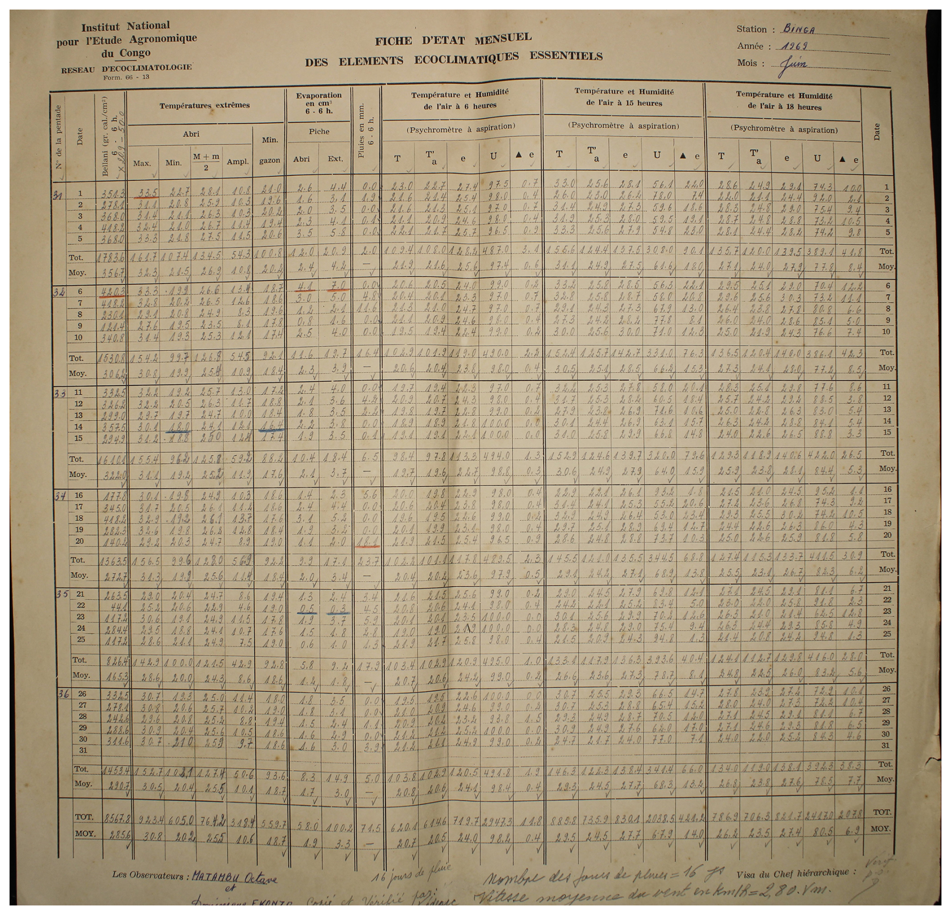
Figure A1 Observed weather data sheet for June 1969 at Station Binga (2°18^′ N, 20°30^′ E) in DRC available within the archives of INERA, Yangambi. Refer to Fig. 1 for the table structure information.

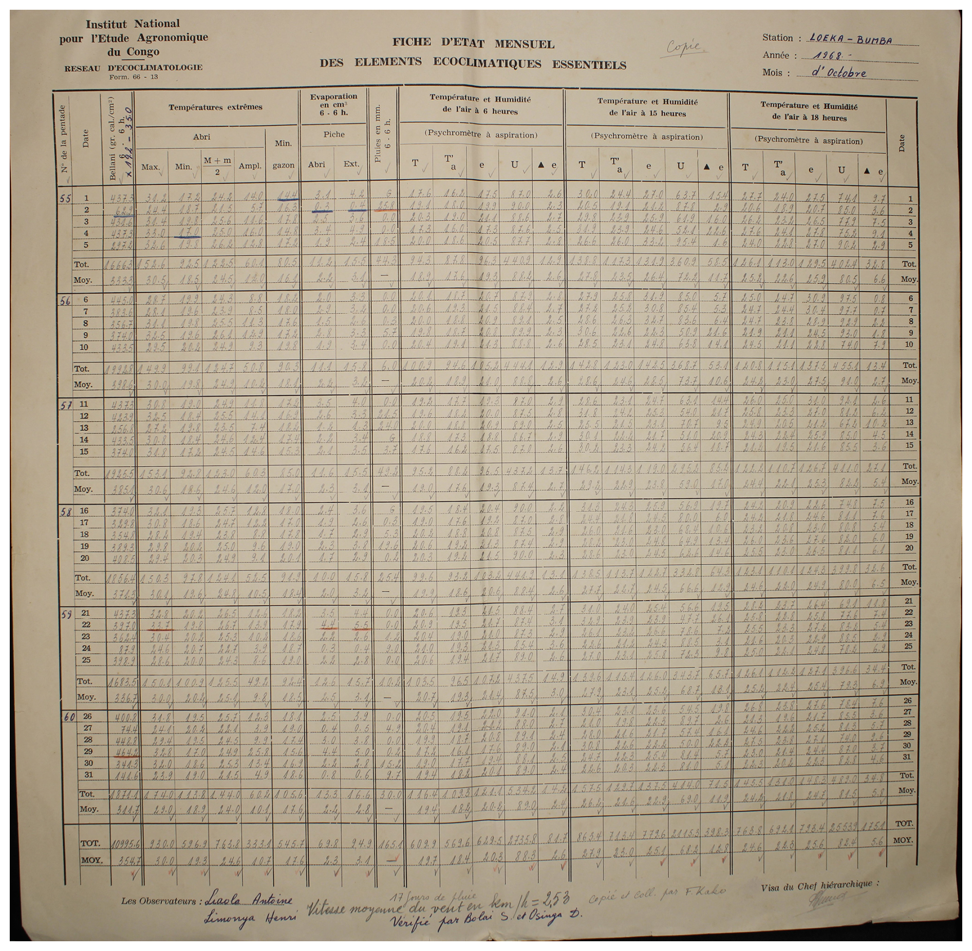
Figure A2 Observed weather data sheet for October 1968 at Station Loeka-Bumba (2°15^′ N, 22°49^′ E) in DRC available within the archives of INERA, Yangambi. Refer to Fig. 1 for the table structure information.

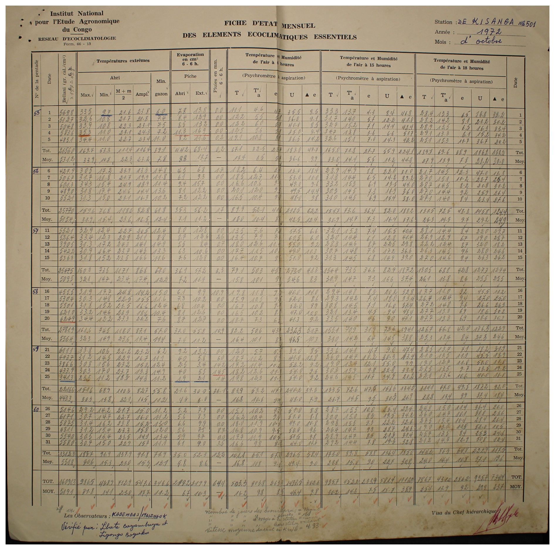
Figure A3 Observed weather data sheet for October 1972 at Station Kisanga-Plateau (11°44^′ S, 27°25^′ E) in DRC available within the archives of INERA, Yangambi. Refer to Fig. 1 for the table structure information.

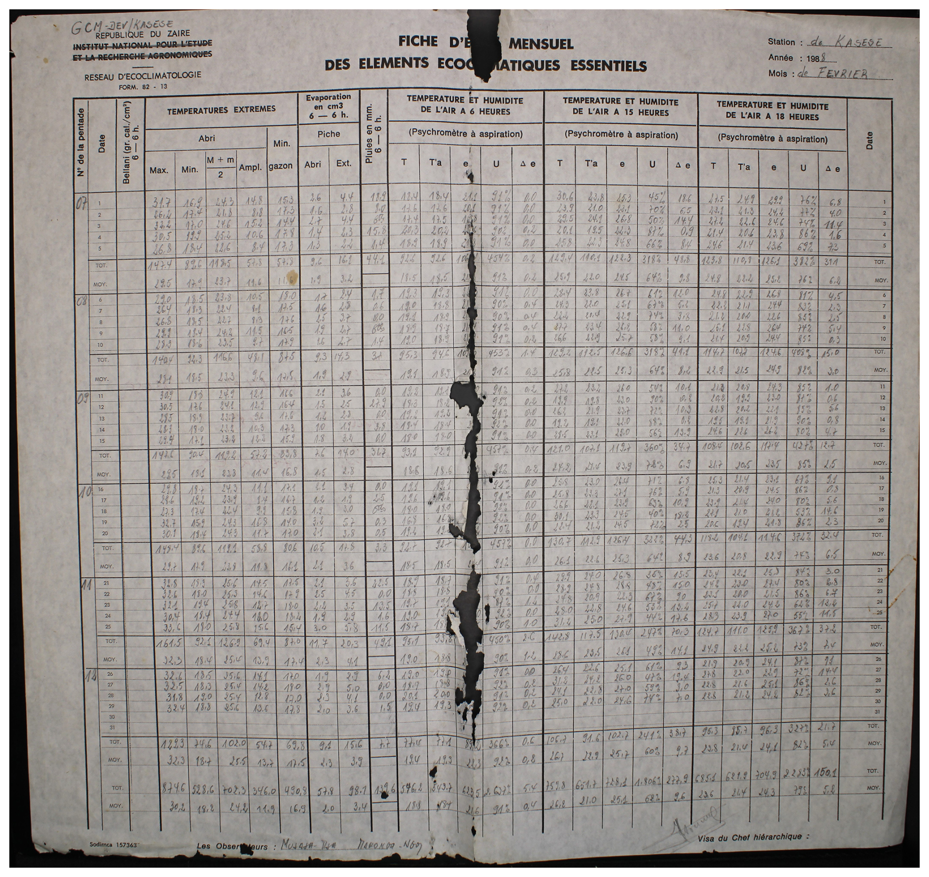
Figure A4 Observed weather data sheet for February 1988 at Station Kaniama-Kasese in DRC available within the archives of INERA, Yangambi. Refer to Fig. 1 for the table structure information.

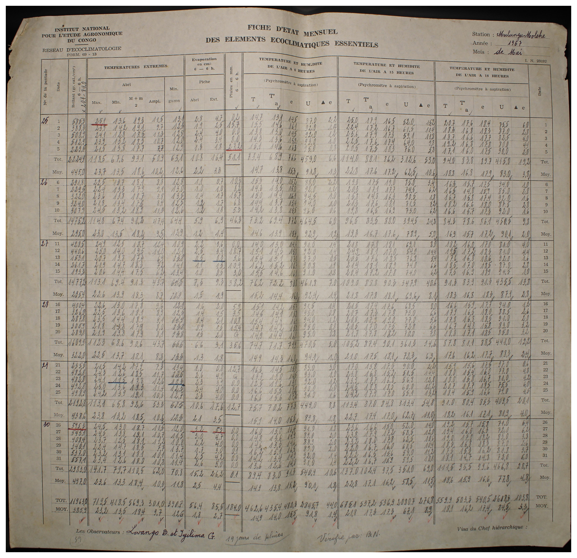
Figure A5 Observed weather data sheet for May 1967 at Station Mulungu-Mulohe (2°18^′ S, 28°47^′ E) in DRC available within the archives of INERA, Yangambi. Refer to Fig. 1 for the table structure information.

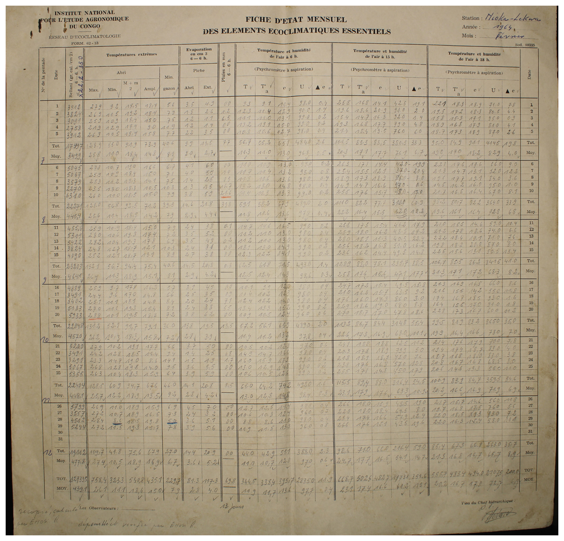
Figure A6 Observed weather data sheet for February 1964 at Station Nioka-Lekwa (2°07^′ N, 30°38^′ E) in DRC available within the archives of INERA, Yangambi. Refer to Fig. 1 for the table structure information.

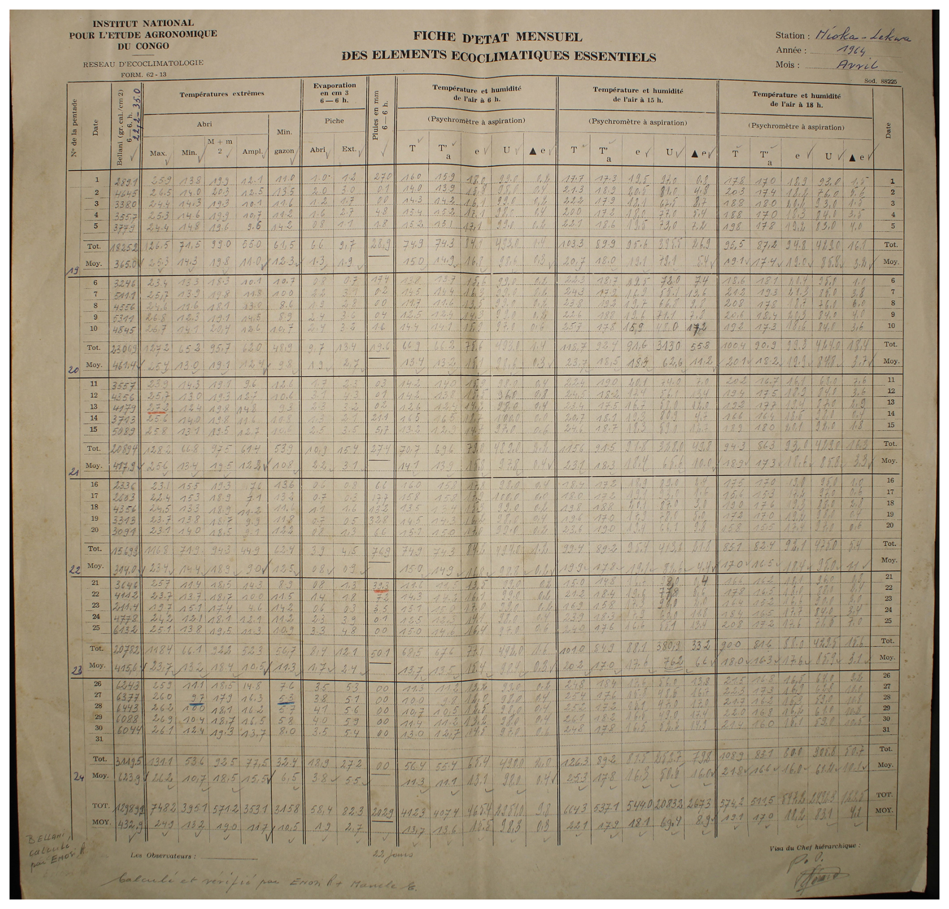
Figure A7 Observed weather data sheet for April 1964 at Station Nioka-Lekwa (2°07^′ N, 30°38^′ E) in DRC available within the archives of INERA, Yangambi. Refer to Fig. 1 for the table structure information.

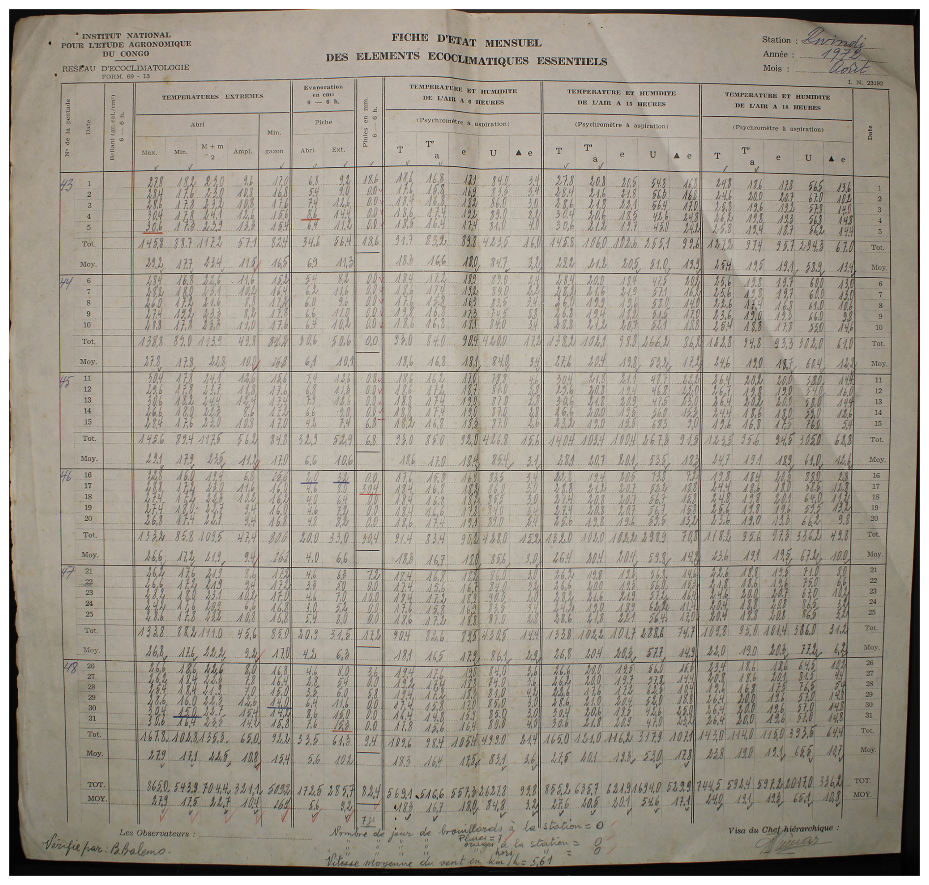
Figure A8 Observed weather data sheet for August 1972 at Station Rwindi (0°47^′ S, 29°17^′ E) in DRC available within the archives of INERA, Yangambi. Refer to Fig. 1 for the table structure information.

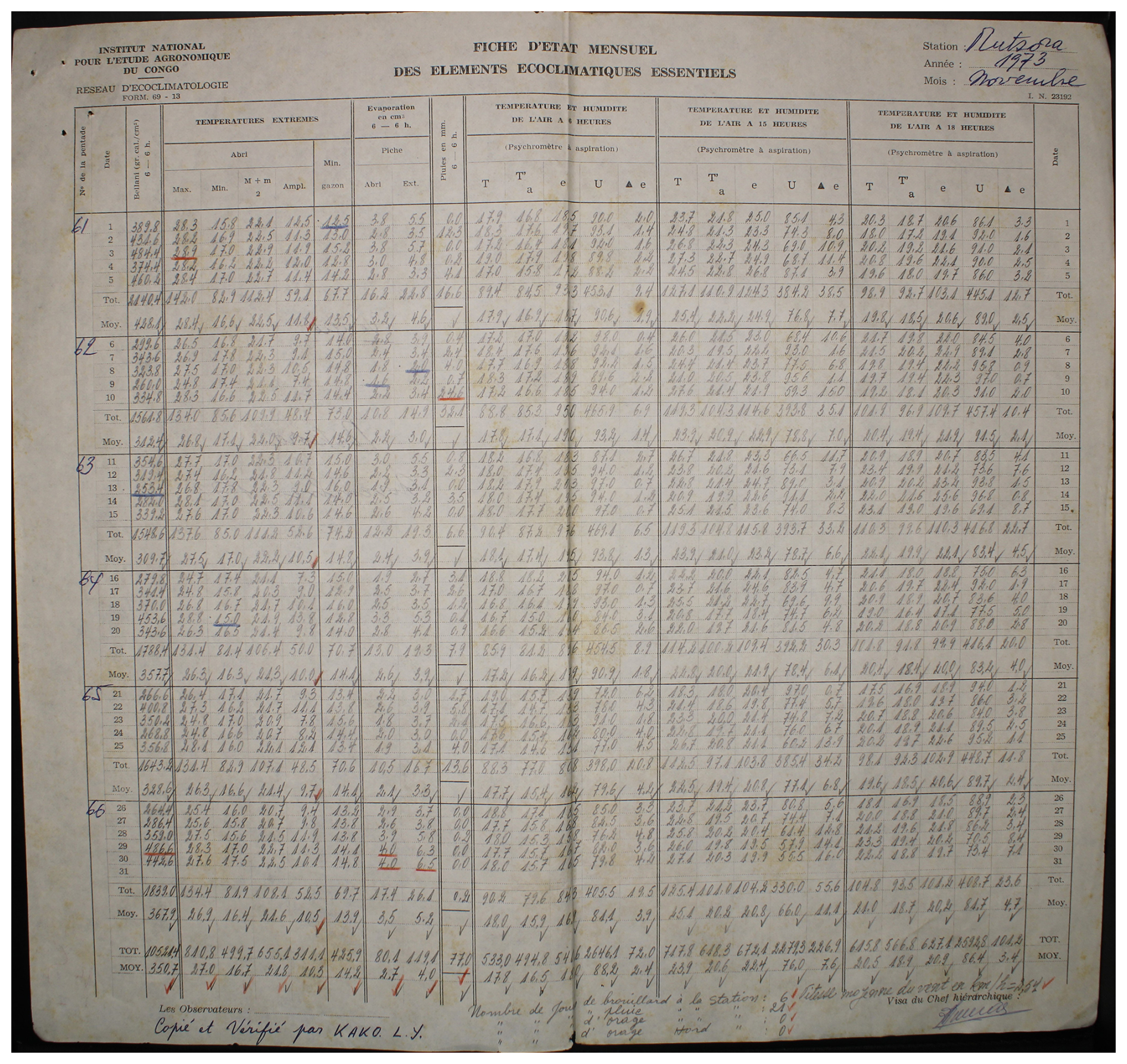
Figure A9 Observed weather data sheet for November 1973 at Station Mutsora (0°19^′ N, 29°44^′ E) in DRC available within the archives of INERA, Yangambi. Refer to Fig. 1 for the table structure information.

Appendix B: Post QA/QC transcribed values of daily maximum, minimum and average temperature, and diurnal temperature range, using MeteoSaver v1.0

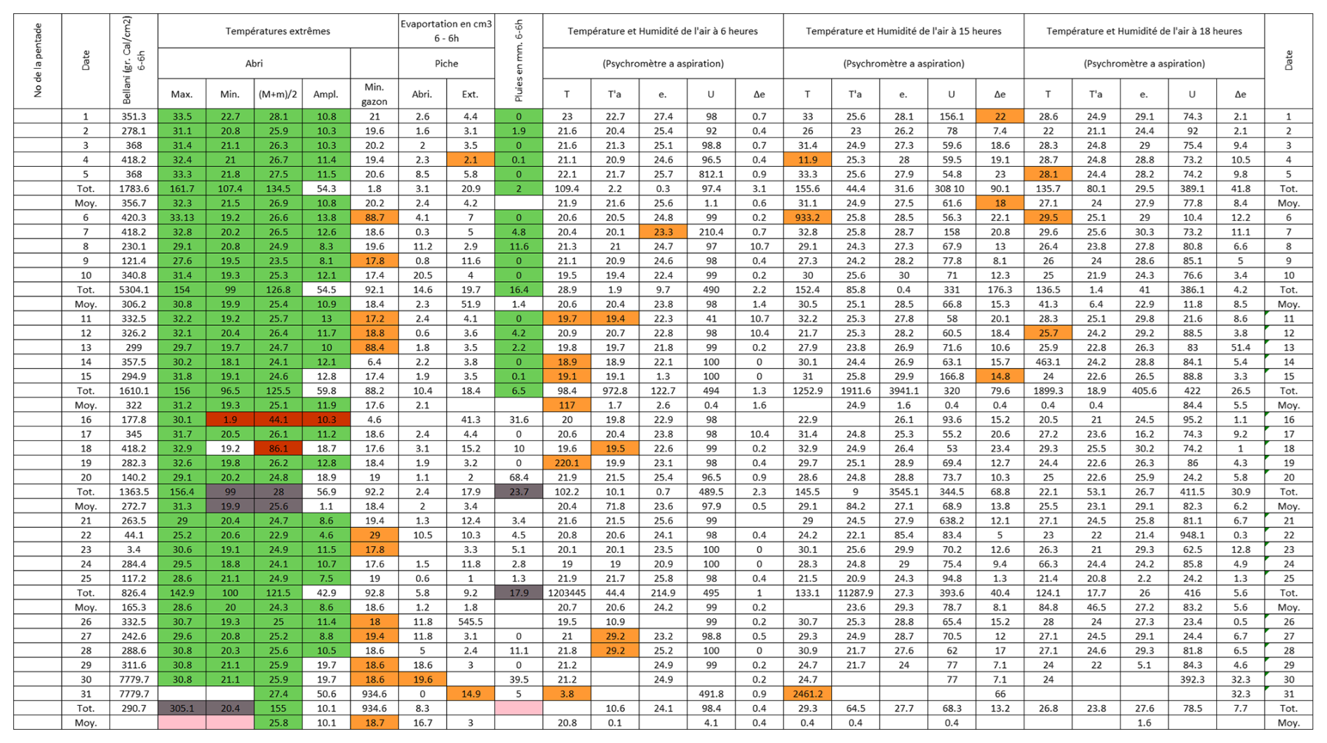
Figure B1 Post-quality controlled table using MeteoSaver, showing confirmed values of daily maximum, minimum and average temperature, diurnal temperature range, and daily precipitation (highlighted in green) for the Station Binga in June 1969 (Fig. A1). The description of the colors in the post-quality controlled table is given in Fig. 10.

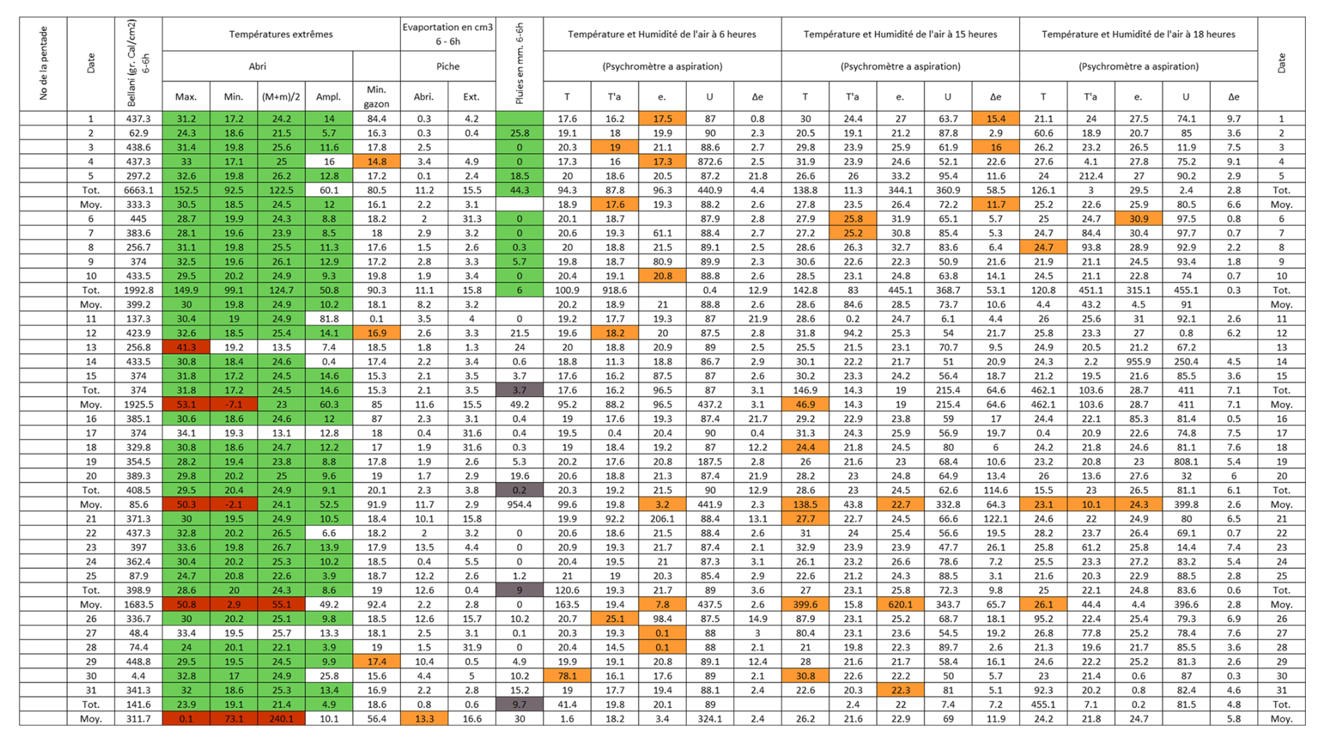
Figure B2 Post-quality controlled table using MeteoSaver, showing confirmed values of daily maximum, minimum and average temperature, diurnal temperature range, and daily precipitation (highlighted in green) for the Station Loeka-Bumba in October 1968 (Fig. A2). The description of the colors in the post-quality controlled table is given in Fig. 10.

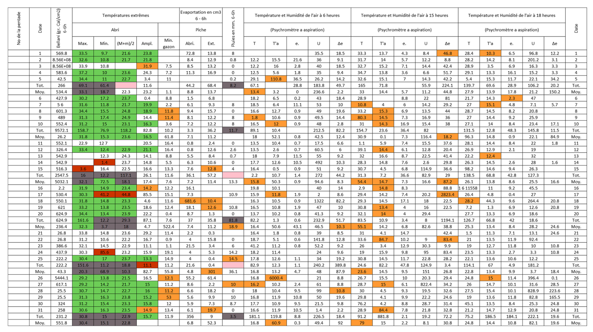
Figure B3 Post-quality controlled table using MeteoSaver, showing confirmed values of daily maximum, minimum and average temperature, diurnal temperature range, and daily precipitation (highlighted in green) for the Station Kisanga-Plateau in October 1972 (Fig. A3). The description of the colors in the post-quality controlled table is given in Fig. 10.

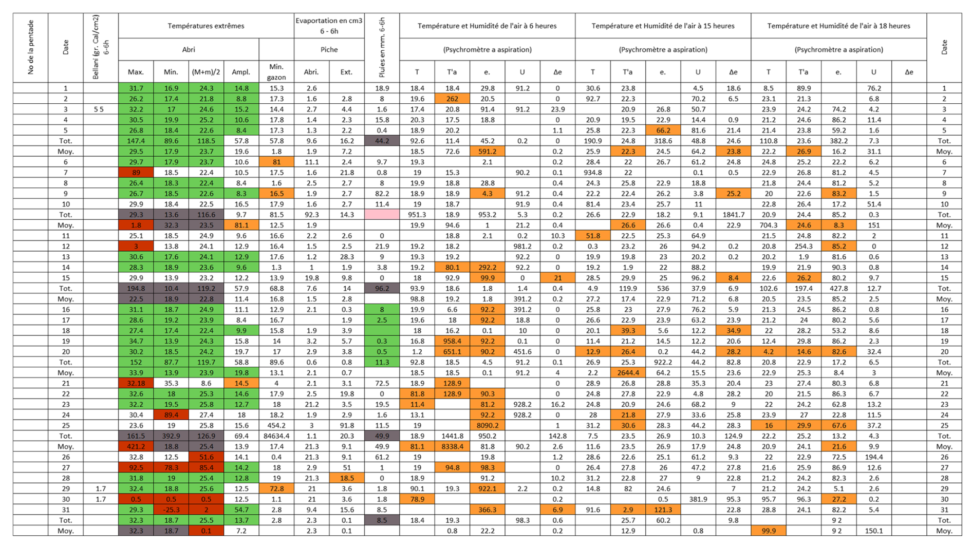
Figure B4 Post-quality controlled table using MeteoSaver, showing confirmed values of daily maximum, minimum and average temperature, diurnal temperature range, and daily precipitation (highlighted in green) for the Station Kaniama-Kasese (Fig. A4). The description of the colors in the post-quality controlled table is given in Fig. 10.

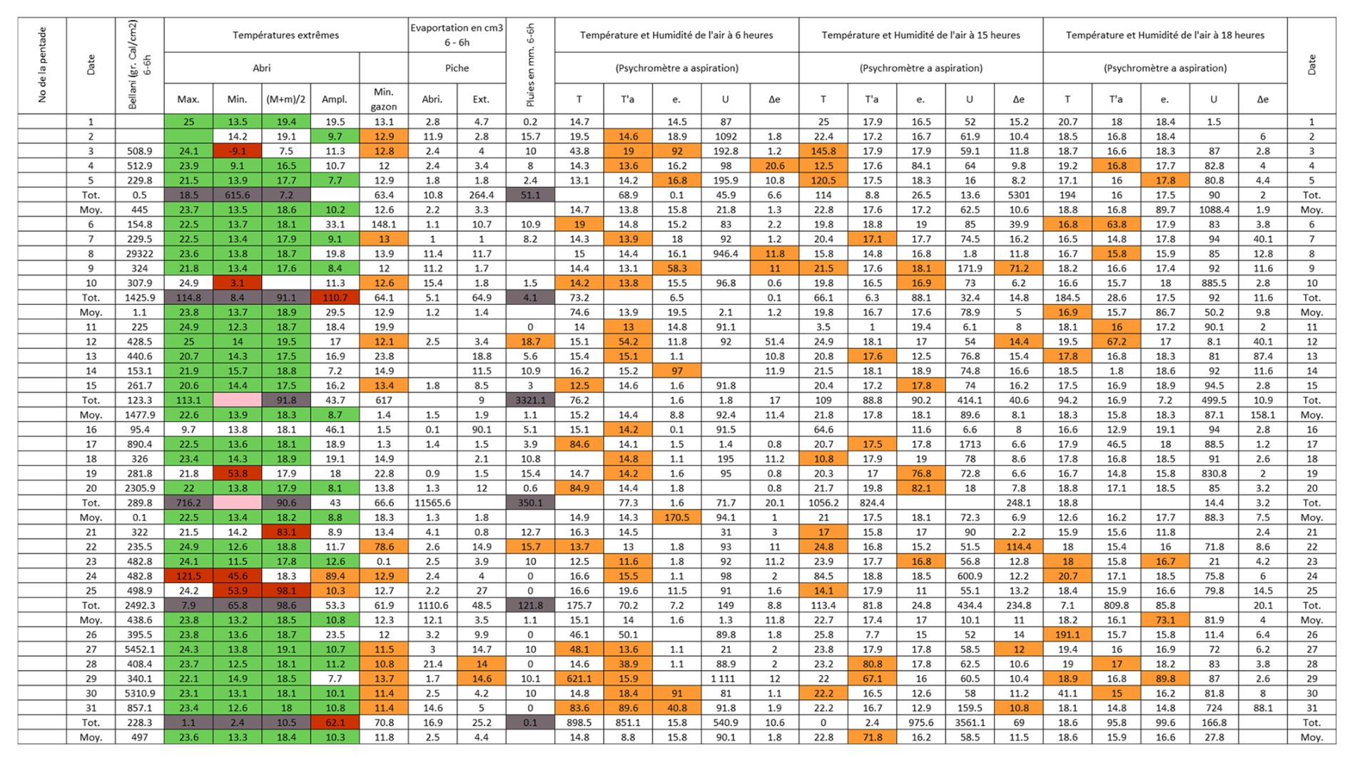
Figure B5 Post-quality controlled table using MeteoSaver, showing confirmed values of daily maximum, minimum and average temperature, diurnal temperature range, and daily precipitation (highlighted in green) for the Station Mulungu-Mulohe in May 1967 (Fig. A5). The description of the colors in the post-quality controlled table is given in Fig. 10.

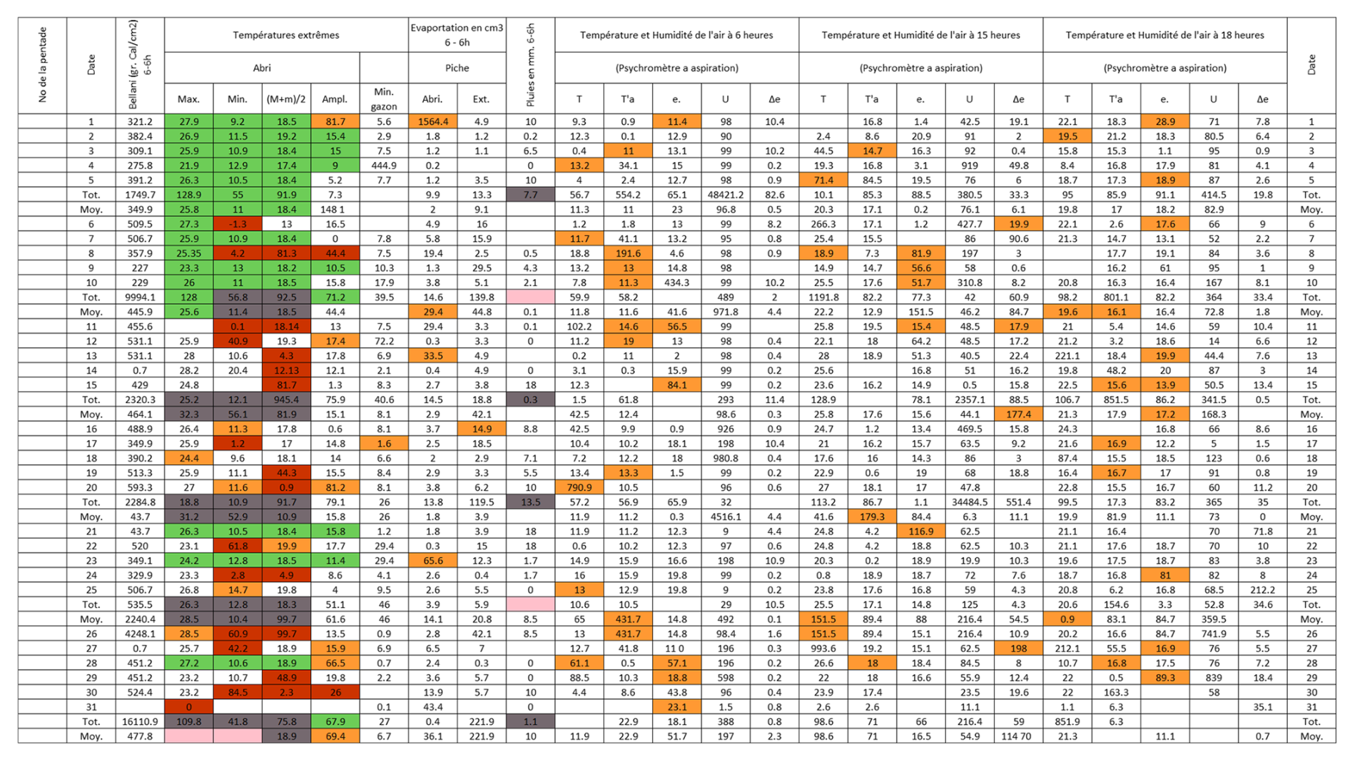
Figure B6 Post-quality controlled table using MeteoSaver, showing confirmed values of daily maximum, minimum and average temperature, diurnal temperature range, and daily precipitation (highlighted in green) for the Station Nioka-Lekwa in February 1964 (Fig. A6). The description of the colors in the post-quality controlled table is given in Fig. 10.

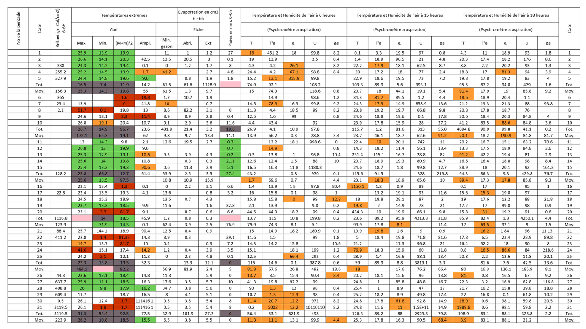
Figure B7 Post-quality controlled table using MeteoSaver, showing confirmed values of daily maximum, minimum and average temperature, diurnal temperature range, and daily precipitation (highlighted in green) for the Station Nioka-Lekwa in April 1964 (Fig. A7). The description of the colors in the post-quality controlled table is given in Fig. 10.

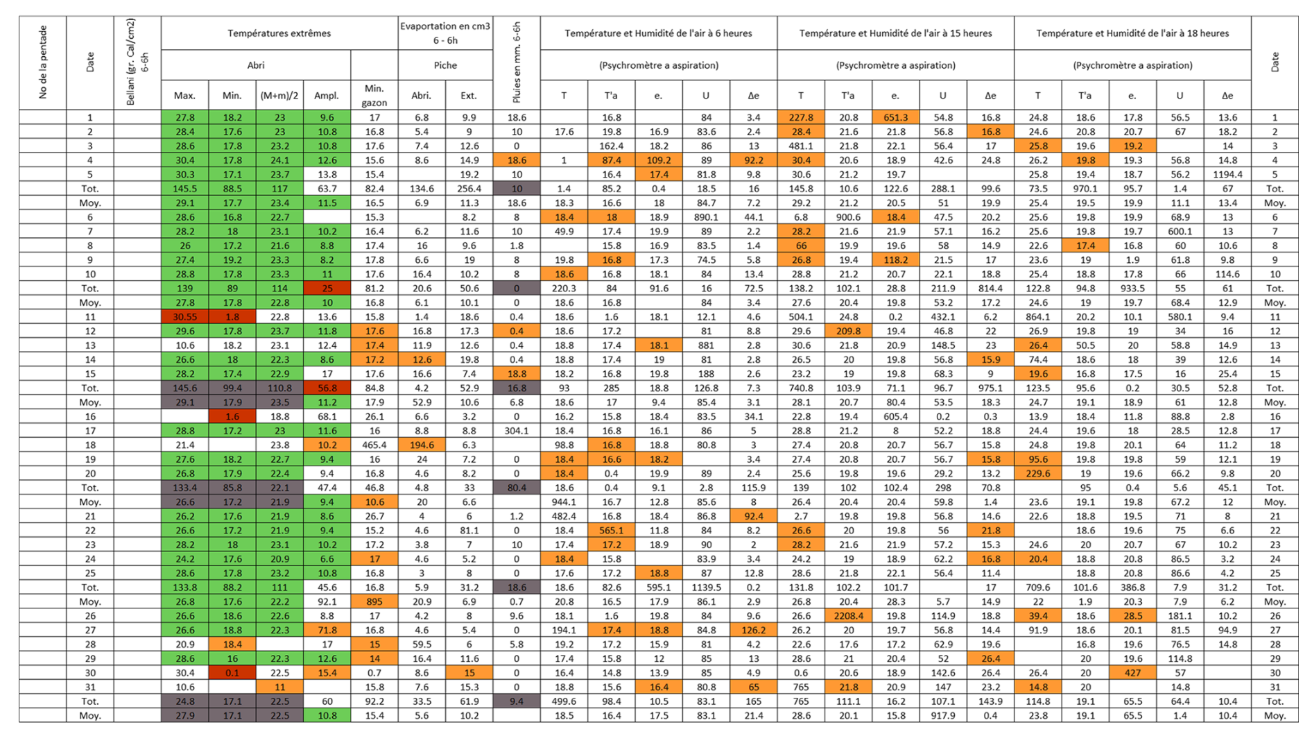
Figure B8 Post-quality controlled table using MeteoSaver, showing confirmed values of daily maximum, minimum and average temperature, diurnal temperature range, and daily precipitation (highlighted in green) for the Station Rwindi in August 1972 (Fig. A8). The description of the colors in the post-quality controlled table is given in Fig. 10.

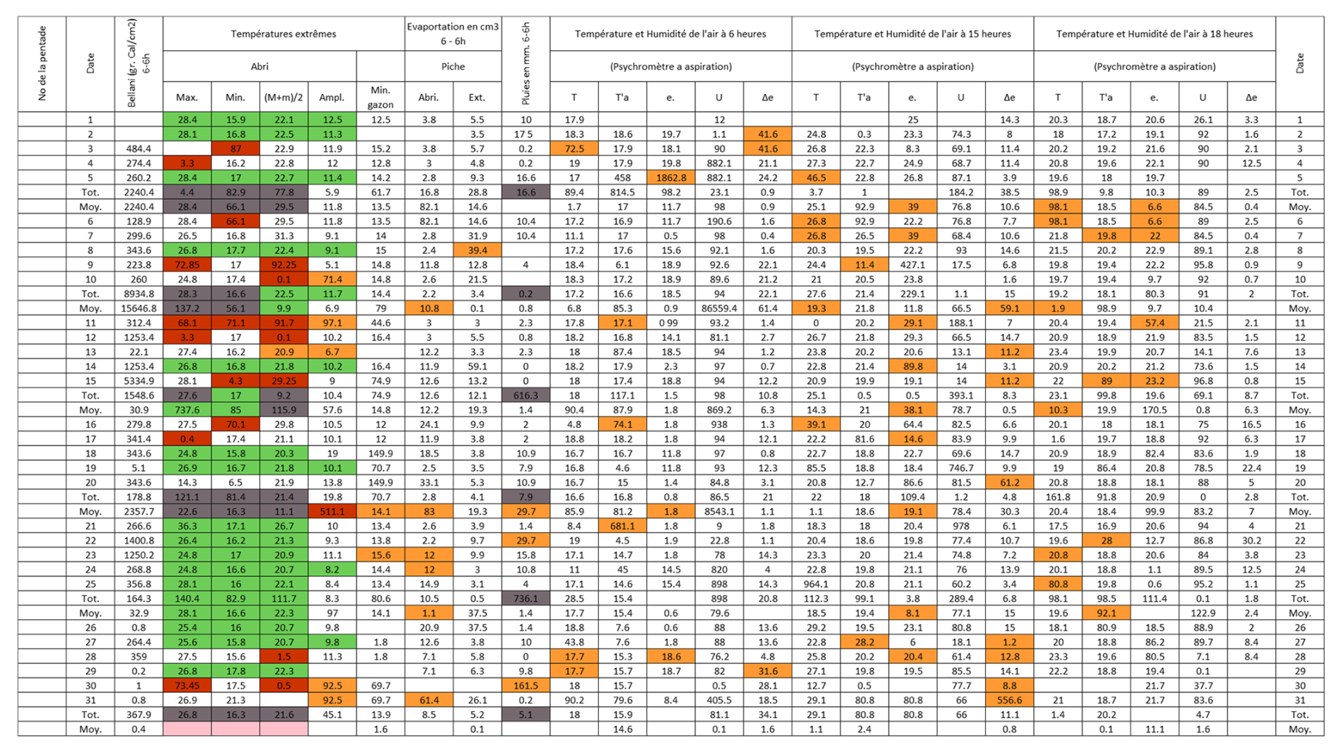
Figure B9 Post-quality controlled table using MeteoSaver, showing confirmed values of daily maximum, minimum and average temperature, diurnal temperature range, and daily precipitation (highlighted in green) for the Station Mutsora in November 1973 (Fig. A9). The description of the colors in the post-quality controlled table is given in Fig. 10.