Numerical strategies for representing Richards' equation and its couplings in snowpack models

The physical processes of heat conduction, liquid water percolation, and phase changes govern the transfer of mass and energy in snow. They are therefore at the heart of any physics-based snowpack model. In the last decade, the use of Richards' equation has been proposed to better represent liquid water percolation in snow. While this approach allows the explicit representation of capillary effects, it can also be problematic as it usually presents a large increase in numerical complexity and cost. This notably arises from the problem of applying a water retention curve in a fully-dry medium such as snow, leading to a divergence and degeneracy in Richards' equation. Moreover, the difficulty of representing both dry and wet snow in a single framework hinders the concomitant solving of heat conduction, phase changes, and liquid percolation. Rather, current models employ a sequential approach, which can be subject to non-physical overshoots. To treat these problems, we propose the use of a regularized water retention curve (WRC) that can be applied to dry snow. Combined with a variable switch technique, this opens the possibility of solving the energy and mass budgets in a fully consistent and tightly coupled manner, whether the snowpack contains dry and/or wet regions. To assess the behavior of the proposed scheme, we compare it to other implementations based on loose-coupling between processes and on the state-of-the-art strategies in snowpack models. Results show that the use of a regularized WRC with a variable switch greatly improves the robustness of the numerical implementation, consistently allowing timesteps greater or equal to 900 s, which results in faster and cheaper simulations. Furthermore, the possibility of solving the physical process in a fully-coupled and concomitant manner results in a slightly reduced error level compared to implementations based on the traditional sequential treatment. However, we did not observe any numerical oscillations and/or divergence sometimes associated with a sequential treatment. This indicates that a sequential treatment remains a potentially interesting tradeoff, favoring computational cost for a small decrease in precision.

1 Introduction

The wetting of snowpacks is a crucial stage in their evolution over time, with direct impacts on their environment. Notably, the intensity and timing of melt runoff have strong implications for the water availability in hydrological basins (Hock et al., 2019; Barnhart et al., 2020). Similarly, the quantification of wet snow avalanche hazard relies on a precise determination of the liquid water content in snowpacks and of the depth of the percolation front (Baggi and Schweizer, 2009; Eckert et al., 2024). Liquid water percolation also plays a crucial role in the formation of ice lenses and crusts (Wever et al., 2016; Quéno et al., 2020), with direct implications for the local ecosystems (Tyler, 2010; Hansen et al., 2010). In this context, numerical snowpack models play a key role to assess the melting and wetting of snowpacks in various locations and under various conditions.

A simple and commonly employed way of representing liquid water percolation in 1D snowpack models is the so-called bucket-scheme. In this picture, snow layers are expected to retain liquid water until a certain threshold, after which all liquid water is instantaneously transferred downward (Bartelt and Lehning, 2002; Vionnet et al., 2012; Sauter et al., 2020). While this implementation is numerically efficient, it cannot capture certain effects, such as capillary barriers, capillary rise, or the finite dynamics of the percolation process. On the other hand, a more detailed description of liquid water flow in snowpacks can be achieved by explicitly solving the liquid water budget under gravitational and capillary forces, i.e. Richards' equation (Richards, 1931; Colbeck, 1974; Illangasekare et al., 1990; Daanen and Nieber, 2009). Richards' equation has for instance been implemented in the detailed 1D models SNOWPACK (Wever et al., 2014) and Crocus (D'Amboise et al., 2017). This more advanced description has notably been shown to better capture the timing associated with the wetting of the snowpack (Wever et al., 2015). In the case of significantly wet snow, capillary forces become negligible and the driving force of liquid water flow reduces to gravity only (Colbeck, 1972). This offers a simplified version of Richards' equation, for instance implemented in the SNTHERM 1D model (Jordan, 1991). However, note that implementations based on the standard 1D Richards' equation cannot represent preferential flow, which is crucial to fully capture the complexity of liquid water percolation in snowpacks (Marsh and Woo, 1985; Schneebeli, 1995; Waldner et al., 2004). Explicit representations of preferential flow in snow have been proposed in the literature. A first broad class of strategies is based on modelling the snowpack in multi-dimensions, allowing the formation of fingering flows in response to snow heterogeneities (Hirashima et al., 2014; Leroux and Pomeroy, 2017; Leroux et al., 2020) and/or instabilities in the wetting front (Moure et al., 2023). These studies offer valuables insights on the physical mechanisms responsible for the formation of preferential flow in snow. A second strategy, which is compatible with a 1D framework, is the use of a dual-domain percolation model (Wever et al., 2016; Quéno et al., 2020).

For all those implementations based on Richards' equation, the simple bucket-scheme is replaced by one or more partial differential equations of liquid water mass budget, with flow driven by capillary and gravitational forces. However, Richards' equation can be notoriously difficult to solve numerically, due to its non-linearities and potential degeneracy (Farthing and Ogden, 2017). Notably, it is usually associated with an adaptive time stepping strategy (e.g. Celia et al., 1990; Forsyth et al., 1995; Wever et al., 2014; D'Amboise et al., 2017), as the use of iterative methods to solve non-linear equations can fail at large timesteps. Therefore, the implementation of Richards' equation in snowpack models can imply a significant increase in numerical cost, hindering its broad use, in particular for simulations over large areas and long periods. For instance, the current implementation of Richards' equation in the detailed snowpack model Crocus (D'Amboise et al., 2017) is known to display signs of numerical instabilities and to require small timesteps of the order of 30 s or less (D'Amboise et al., 2017, and M. Lafaysse, personal communication, 2024), while the model is usually run with a 900 s timestep. This drastically hinders the routine use of Richards' equation in Crocus, as the two-order of magnitude increase in numerical cost can be considered as a too expensive trade-off. Moreover, due to the difficulty of representing both dry and wet snow in a unified framework for Richards' equation, current implementations in snowpack models assume that a small amount of liquid water is always present and need to modify the capillary behavior of snow in consequence (Wever et al., 2014; D'Amboise et al., 2017). This lack of unified treatment of dry and wet snow hinders the concomitant numerical solving of liquid water percolation with other physical processes (such as phase change or heat conduction). Rather, Richards' equation is usually solved sequentially, (Wever et al., 2014; D'Amboise et al., 2017) whereas the processes are inextricably coupled in actual snowpacks (Daanen and Nieber, 2009).

The main goal of this article is to investigate how the specific numerical implementation of liquid water percolation in snow affects the behavior of snowpack models, with a focus on their robustness and numerical cost. For this, we rely on various techniques proposed in applied mathematics, where the efficient solving of Richards' equation has been an active research subject (e.g. Forsyth et al., 1995; Sadegh Zadeh, 2011; Farthing and Ogden, 2017; Bassetto et al., 2020). Specifically, we explore whether the use of regularized capillary laws and the concomitant solving of Richards' equation with other physical processes are beneficial for the numerical behavior of snowpack models. For simplicity, we restrict our focus to the 1D case without preferential flow. The article is organized as follows. Section 2 presents a consistent system of equations describing energy and mass conservation in snowpacks that applies naturally to both dry and wet snow. Section 3 presents toy-models based on different numerical implementations of the heat and mass budget equations and on the standard implementations used in state-of-the art detailed snowpack models as well. Simple test cases, representing three distinct situations of liquid water infiltration in snowpacks are presented in Sect. 4. Finally, the performance of the toy-models on these test cases are discussed in Sect. 5.

2 Deriving a consistent system of equations for the energy and mass budgets in snowpacks

While a real snowpack is a complex 3D structure composed of intertwined ice, air, and liquid water, such complexity is challenging to model. Rather, snowpack models rely on a macroscopic and 1D framework (e.g. Jordan, 1991; Bartelt and Lehning, 2002; Vionnet et al., 2012; Sauter et al., 2020). Here, macroscopic means that snow is not treated as an actual multiphasic medium, but rather as a homogeneous material (Torquato, 2002). In this framework, snow is characterized by macroscopic material properties (sometimes referred to as effective properties, as they characterize the behavior of the porous medium treated as an equivalent homogeneous material; Auriault et al., 2009), such as its thermal capacity (Calonne et al., 2014) or its hydraulic conductivity (Calonne et al., 2012).

The core of any snowpack model thus requires determining and solving the equations governing the evolution of the macroscopic energy and mass contents of snow. This can be done from the first principles of energy and mass conservation, complemented by material laws characterizing the effective material properties. As we focus this article on liquid water percolation, we neglect several processes at play in snowpacks, such as metamorphism or water vapor transport, in order to simplify our analysis. The goal of this section is to present a set of equations that govern the physical evolution of a snowpack and that apply both in dry and wet snow. Note that while this article assumes a 1D framework, as usually done in snowpack models, it could be transposed to a 2D or 3D configuration similar to what is done in several rock, soil, or even some snowpack models (Vauclin et al., 1979; Hirashima et al., 2014; Leroux and Pomeroy, 2017; Cockett et al., 2018). Therefore, we tried to keep the notation used in this article as general as possible.

2.1 Snow internal energy conservation

As a first equation governing the evolution of a snowpack, we consider the energy conservation of snow, understood here as the combination of the ice matrix and the air within (and excluding potential liquid water). The temporal evolution of the snow energy is given by a classical conservation equation, i.e.

$$\begin{array}{}\text{(1)}& {\partial }_t{h}_{\mathrm{s}}+\mathrm{\nabla }\cdot {\mathit{F}}_{\text{cond}}=Q_{\text{abs}}+Q_{\text{freeze}},\end{array}$$

where h_s is the energy content of snow (expressed in J m⁻³), F_cond the heat conduction flux (in W m⁻²), Q_abs a volumetric energy source (in W m⁻³) due to shortwave absorption within the snowpack (van Dalum et al., 2019; Picard and Libois, 2024), and Q_freeze the energy absorbed/released during freezing/melting (in W m⁻³). Moreover, we classically assume that the heat conduction flux F_cond follows Fourier's law

$$\begin{array}{}\text{(2)}& {\mathit{F}}_{\text{cond}}=-\mathit{\lambda }\mathrm{\nabla }T\end{array}$$

where λ is the thermal conductivity of snow (in $\mathrm{W}{\mathrm{K}}^{-\mathrm{1}}{\mathrm{m}}^{-\mathrm{1}}$) and T its temperature (K). These equations, and the value of the snow thermal conductivity in terms of the microstructure, can for instance be derived from homogenization methods (e.g. Boutin et al., 2010; Calonne et al., 2011, 2014; Bouvet et al., 2024). Moreover, the temperature and the energy content are related through the thermal capacity of snow

$$\begin{array}{}\text{(3)}& h_{\mathrm{s}}=\underset{T_{\mathrm{0}}}{\overset{T}{\int }}{c}_p\mathrm{d}T=c_p(T-T_{\mathrm{0}})\end{array}$$

where T₀ is a reference temperature taken as the fusion temperature of ice at standard pressure for simplicity, and c_p is the volumetric thermal capacity of snow (in $\mathrm{J}{\mathrm{m}}^{-\mathrm{3}}{\mathrm{K}}^{-\mathrm{1}}$; Tubini et al., 2021). Note that we have assumed for simplicity that c_p does not depend on temperature, as regularly done in snowpack models (e.g. in the Crocus model; Vionnet et al., 2012). Using homogenization methods, the volumetric thermal capacity of snow can be shown (e.g. Calonne et al., 2014) to be

$$\begin{array}{}\text{(4)}& c_p={\mathit{\varphi }}_{\mathrm{i}}{c}_{\mathrm{i}}+(\mathrm{1}-{\mathit{\varphi }}_{\mathrm{i}})c_{\mathrm{a}}\simeq {\mathit{\varphi }}_{\mathrm{i}}{c}_{\mathrm{i}}\end{array}$$

where ϕ_i is the ice volumetric fraction, and c_i and c_a the volumetric thermal capacity of ice and air, respectively.

2.2 Liquid water conservation

Since the heat budget and temperature of snow are directly related to the melting and freezing of water, it is necessary to also treat the liquid water budget. This can be done with the use of Richards' equation (Wever et al., 2014, 2015, 2016; D'Amboise et al., 2017). Note that in this paper we only consider “matric” water flow, and do not consider fast preferential flow (Vogel et al., 2000; Lewandowska et al., 2004; Wever et al., 2016). This limitation is discussed in Sect. 5.4. Under these conditions, the mass conservation of liquid water is given by

$$\begin{array}{}\text{(5)}& {\mathit{\rho }}_{\mathrm{w}}{\partial }_t{\mathit{\theta }}_{\mathrm{w}}+{\mathit{\rho }}_{\mathrm{w}}\mathrm{\nabla }\cdot {\mathit{F}}_{\mathrm{w}}=-M_{\text{freeze}}\end{array}$$

where θ_w is the volumetric liquid water content (LWC; expressed in m³ of water per m³ of snow), ρ_w the density of liquid water (assumed constant; in kg m⁻³), F_w is the liquid water flux (in m³ of water per m² of snow per s), and M_freeze is the rate of freezing water (counted positive in the case of freezing and expressed in kg of water per m³ of snow per s). The rate of freezing water M_freeze is directly related to the rate of energy release/absorption Q_freeze of Eq. (1) through Q_freeze=L_fusM_freeze, with L_fus the specific enthalpy of fusion of water (in J kg⁻¹).

The liquid water flux is assumed to follow the Darcy-Buckingham law (Sposito, 1978)

$$\begin{array}{}\text{(6)}& {\mathit{F}}_{\mathrm{w}}=-K^{\text{sat}}{k}_{\mathrm{r}}(\mathrm{\nabla }\mathit{\psi }+\cos \mathit{\gamma })\end{array}$$

where K^sat is the saturated hydraulic conductivity (in m s⁻¹), which does not depend on the LWC but only the properties of the ice matrix, k_r the relative hydraulic conductivity, that depends on the LWC, ψ the liquid matric potential (in m and that can be negative due to capillary forces), and γ the slope angle. Note that in the multidimensional case, the gravity term cos γ should be replaced by the unit vector orientated with gravity. In the same way that the snow energy and temperature are related through Eq. (3), the LWC and the matric potential are related through the use of a water retention curve (WRC). This WRC can be expressed with the use of, for instance, the van Genuchten or Brook models (Brooks and Corey, 1964; van Genuchten, 1980; Lenhard et al., 1989). In this article, and consistently with previous snow-related work (Wever et al., 2014; D'Amboise et al., 2017), we use a van Genuchten model for the WRC in snow

$$\begin{array}{}\text{(7)}& {\mathit{\theta }}_{\mathrm{w}}=\left\{\begin{array}{ll}{\mathit{\theta }}_{\mathrm{r}}+({\mathit{\theta }}_{\mathrm{s}}-{\mathit{\theta }}_{\mathrm{r}})(\mathrm{1}+|\mathit{\alpha }\mathit{\psi }{|}^n{)}^{\frac{\mathrm{1}-n}{n}}& \text{if }\mathit{\psi }<\mathrm{0}\\ {\mathit{\theta }}_{\mathrm{s}}& \text{otherwise}\end{array}\right.\end{array}$$

where n and α (in m⁻¹) are parameters characterizing the shape of the WRC and which depends on the snow microstructure (Yamaguchi et al., 2012), and θ_r and θ_s are referred to as the residual and saturation LWC, respectively. Physically, θ_s corresponds to the maximum amount of liquid water a snow sample can hold (thus typically assumed to correspond to the total porosity), and θ_r to the minimum amount of water that can be reached with draining through capillary and gravity forces.

To solve Richards' equation, it is also necessary to provide an expression for the dependence of the relative hydraulic conductivity k_r on the liquid water content. Following Mualem (1976), in complement of the van Genuchten WRC, the hydraulic conductivity is usually taken as

$$\begin{array}{}\text{(8)}& k_{\mathrm{r}}=\sqrt{S}{\left({\displaystyle \frac{{\int }_{\mathrm{0}}^S\frac{\mathrm{d}S}{\mathit{\psi }}}{{\int }_{\mathrm{0}}^{\mathrm{1}}\frac{\mathrm{d}S}{\mathit{\psi }}}}\right)}^{\mathrm{2}}=\sqrt{S}{\left(\mathrm{1}-{\left(\mathrm{1}-S^{\frac{n}{n-\mathrm{1}}}\right)}^{\frac{n-\mathrm{1}}{n}}\right)}^{\mathrm{2}}\end{array}$$

where $S=\frac{{\mathit{\theta }}_{\mathrm{w}}-{\mathit{\theta }}_{\mathrm{r}}}{{\mathit{\theta }}_{\mathrm{s}}-{\mathit{\theta }}_{\mathrm{r}}}$ is referred to as the saturation degree. It can be noted that the relative hydraulic conductivity is an increasing function of θ_w that vanishes at the residual LWC θ_r and reaches unity value at water saturation.

However, Richards' equation presents specific problems in the case of water-saturated and fully-dry materials. In the case of a water-saturated material, the liquid water content reaches a maximum value, while the matric potential can keep increasing. In other words, in the saturated case, the equation becomes degenerate and can no longer be expressed in terms of liquid water content. This is a classical difficulty associated with Richards' equation, usually circumvented by using ψ as the primary variable to describe the material (Celia et al., 1990; Farthing and Ogden, 2017). It can also be treated using a variable switch technique, effectively changing from θ_w to ψ as a primary variable depending on the degree of saturation of the material (Diersch and Perrochet, 1999; Krabbenhøft, 2007; Bassetto et al., 2022). This latter technique is explored below in the article. The problem of a fully-dry material is more specific to snow, and requires a dedicated treatment.

The problem of Richards' equation for dry snow

Indeed, in their usual forms, the WRCs used as material laws in Richards' equation do not apply in dry snow. In Eq. (7), the matric potential ψ diverges when the LWC approaches its residual value θ_r. In material solely driven by capillary and gravity flow, this implies that θ_w cannot drop below this residual value, i.e. that liquid water is always present. To the contrary, snow can become fully dry when energy is removed and the residual liquid water freezes. In such a case, the LWC can fall below the residual liquid water content and even vanish. Then, the matric potential ψ becomes undefined. The use of a WRC with a hysteresis distinguishing the drying and wetting curves (for instance as in Leroux and Pomeroy, 2017) could partially mitigate this problem, as wetting curves can reach a vanishing LWC (Bouvet et al., 2025). However, even in this case, the issue of a diverging WRC at a finite LWC remains a problem for drying snow. In snowpack models, this issue of dry snow has been circumvented in previous implementations of Richards' equation by keeping a small liquid water content, even in the case of snow below the fusion temperature (Wever et al., 2014; D'Amboise et al., 2017). This however hinders a consistent treatment of coupled heat and liquid water budget, as snow below the fusion is considered dry while solving the heat budget but wet while solving the liquid water budget. Furthermore, this technique requires the residual LWC to be artificially modified, in order to remain strictly below the liquid water content at all times. If this modified residual LWC is applied to both the WRC and the hydraulic conductivity, snow containing very little liquid water will tend to percolate, even though the unmodified WRC would rather imply that the liquid water should be held still under capillary forces. Percolation could be stopped by keeping a hydraulic conductivity that vanishes at the residual point, but the physical link between the WRC and the hydraulic conductivity (Mualem, 1976) would then be partially lost.

This issue of the disappearance of a phase and of the divergence of the capillary forces is not only encountered in snow modeling. It is for instance present in underground nuclear-waster storage, where phases can appear and disappear (e.g. Bourgeat et al., 2009). To the best of our knowledge, two types of solutions to this problem have been proposed. First, the gradient of matric potential can be rewritten in terms of the gradient of liquid water content using the chain-rule (similarly to Bourgeat et al., 2009). The liquid water flux is thus taken as $-K^{\text{sat}}{k}_{\mathrm{r}}(\mathrm{\nabla }\mathit{\psi }+\cos (\mathit{\gamma }\left)\right)=-K^{\text{sat}}{k}_{\mathrm{r}}({\partial }_{{\mathit{\theta }}_{\mathrm{w}}}\mathit{\psi }\mathrm{\nabla }{\mathit{\theta }}_{\mathrm{w}}+\cos (\mathit{\gamma }\left)\right)$. While the derivative ${\partial }_{{\mathit{\theta }}_{\mathrm{w}}}\mathit{\psi }$ diverges near the residual point, the product $-K^{\text{sat}}{k}_{\mathrm{r}}{\partial }_{{\mathit{\theta }}_{\mathrm{w}}}\mathit{\psi }$ vanishes near the residual point (as k_r rapidly goes to zero). This product can thus be extended at and below the residual point with a value of zero, allowing the computation of the liquid water flux to be defined at and below the residual point. However, using this technique for the computation of the liquid water flux presents one main issue. The use of the liquid water content gradient as the driving force for the liquid water flux implies that the state of equilibrium is characterized by a uniform liquid water content rather than uniform water (matric + gravitational) potential. While this is not a problem in the case of a homogeneous medium, it will negatively impact the representation of capillary barriers in a stratified medium, unless a specific treatment is implemented at the interfaces between the different strata (Amaziane et al., 2012). This is a major issue for stratified snowpack, as capillary barriers are crucial features that need to be captured (Wever et al., 2016). The second technique proposed in the literature to circumvent the singularity of the WRC near the residual point is to regularize it, so that it does not diverge (Beaude et al., 2019; Moure et al., 2023). The matric potential simply assumes a finite value near and below the residual point.

For our article, we rely on the second technique, namely the regularization of the WRC. Concretely, this is done by limiting the divergence of the retention curve up to a critical liquid water content θ_lim and thus a corresponding limit matric potential ψ_lim. Below that point, the liquid water content is allowed to further decrease (down to 0 in the case of fully dry and cold snow) while the matric potential remains at the value ψ_lim. This was done by choosing a unique limit saturation degree $S_{\text{lim}}=\frac{{\mathit{\theta }}_{\text{lim}}-{\mathit{\theta }}_{\mathrm{r}}}{{\mathit{\theta }}_{\mathrm{s}}-{\mathit{\theta }}_{\mathrm{r}}}$, applied to all snow, below which the WRC reaches its plateau. Some regularized WRC are depicted in Fig. 1 for three different snow samples. The value of S_lim needs to be taken small (typically 10⁻¹⁰), in order not to restrict too much the sharp increase of the matric potential at low LWCs. With this modification of the WRC, θ_lim assumes a role similar to that of the residual value: it corresponds to the point that cannot be further dried with water flow alone. To be consistent with this idea, we propose also to modify the expression of the relative hydraulic conductivity such that it vanishes at θ_lim rather than θ_r. Specifically, we take

$$\begin{array}{}\text{(9)}& k_{\mathrm{r}}=\left\{\begin{array}{ll}\sqrt{S}{\left(\frac{{\int }_{S_{\text{lim}}}^S\frac{\mathrm{d}S}{\mathit{\psi }}}{{\int }_{S_{\text{lim}}}^{S_{\mathrm{s}}}\frac{\mathrm{d}S}{\mathit{\psi }}}\right)}^{\mathrm{2}}=\sqrt{S}{\left(\mathrm{1}-{\left(\frac{\mathrm{1}-S^{\frac{n}{n-\mathrm{1}}}}{\mathrm{1}-S_{\text{lim}}^{\frac{n}{n-\mathrm{1}}}}\right)}^{\frac{n-\mathrm{1}}{n}}\right)}^{\mathrm{2}}& \\ & \mathrm{\text{if}}S>S_{\text{lim}}\\ \mathrm{0}& \mathrm{\text{otherwise}}\end{array}\right.\end{array}$$

which vanishes when θ_w=θ_lim. As θ_lim corresponds to the point where liquid cannot flow anymore, we refer to as it as the retention point, to distinguish it from the residual point θ_r. Note that while we have constructed the regularization as a plateau, other choices could be made. For instance, the WRC could be regularized through a linear function (Moure et al., 2023). With the help of regularized WRCs, Richards' equation now applies to both dry and wet snow, and can naturally handle regime changes between them.

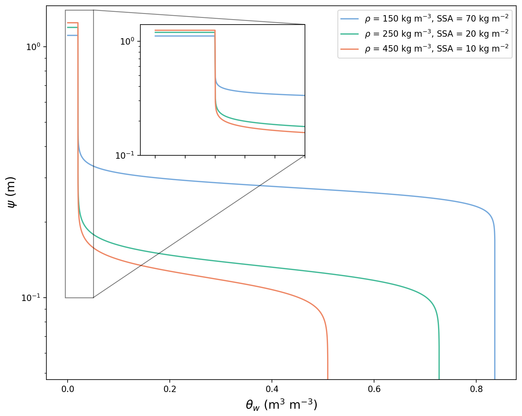
Figure 1 Examples of the regularized water retention curves used in this work, for three different snow density and surface specific area (SSA). The zoomed insert focuses on the regularization and the associated plateau below the retention point.

2.3 Ice budget

Besides the energy and liquid water budgets, the process of water melting and freezing needs to be accounted for in the ice budget to properly close the mass budget. There are two potential ways to account for a melting or refreezing event in the ice budget while respecting mass balance: it can be either viewed as a decrease or increase in density at constant volume, or as a loss or gain of volume at constant density. Depending on the snowpack model, these two possibilities have been employed to represent melt. For instance, melt is treated as a decrease of thickness at constant density in the Crocus model (Vionnet et al., 2012) and a decrease of density at constant thickness in SNOWPACK (Bartelt and Lehning, 2002). The justification for the former choice follows the observation that melting snow is usually of a high density, and thus that the melting process should not act as a de-densification mechanism. Yet, as phase changes occur directly within the snow microstructure, at the surface of the porous ice matrix, we rather believe that both melting and refreezing impact the snow density, without direct impact on the thickness, as done in the SNOWPACK model. With this idea, the relatively high-density nature of melting snow could be attributed to the low viscosity of wet snow (Vionnet et al., 2012) that easily compacts under mechanical stress. Therefore, for the rest of the paper we assume that both type of phase changes affect the snow density, and not directly the snow layer thicknesses. The ice mass budget within the snowpack is thus given by

$$\begin{array}{}\text{(10)}& {\mathit{\rho }}_{\mathrm{i}}{\partial }_t{\mathit{\varphi }}_{\mathrm{i}}=M_{\text{freeze}}\end{array}$$

where ϕ_i is the ice volume fraction and ρ_i the ice density (in kg m⁻³).

2.4 Resulting equations

In order to close the system of equations, it is necessary to provide an expression for the freezing rate M_freeze. This is done by defining both the thermodynamical equilibrium between ice and liquid water and the dynamics with which this equilibrium is restored. However, to the best of our knowledge, there is no broadly accepted theoretical or experimental work providing the dynamics of melting or freezing of water in snow (Moure et al., 2023). As most snowpack models (e.g. Jordan, 1991; Bartelt and Lehning, 2002; Vionnet et al., 2012; Sauter et al., 2020), we assume (i) that liquid water and the snow are in thermodynamical equilibrium (which means that the melting/freezing dynamics can be assumed as infinitely fast) and (ii) that this equilibrium occurs at the single temperature T₀. However, we note that these assumptions are not systematic in snowpack models. First, the recent article of Moure et al. (2023) proposes to relax the assumption of local thermal equilibrium and to introduce a finite rate of phase change, derived from the upscaling of the Frenkel-Wilson equation. This implies that the ice and liquid water temperatures in a snow sample are in general different and can be above or below the fusion point T₀. This modeling framework, composed of four partial differential equations, is briefly presented in Appendix A. However, as observed in the Appendix, the timescale of relaxation towards local thermodynamical equilibrium appears to be much smaller than the timescale of matric water movement and heat diffusion considered in this manuscript, which supports the standard assumption of local equilibrium in snowpack models. Also, due to capillary effects, the thermal equilibrium between the ice and liquid water phases technically occurs on a temperature range rather than at a single temperature. This effect is commonly taken into account in soil models through a so-called soil Freezing Characteristic Curve (soil FCC; Devoie et al., 2022). Some snowpack models have proposed to introduce a similar FCC for snow (Daanen and Nieber, 2009; Dutra et al., 2010; Clark et al., 2017). While the FCC of snow could in principle be computed from the WRC of Sect. 2.2 (as done for instance in Daanen and Nieber, 2009; Li et al., 2023), this would represent a significant increase in the complexity of the snow representation. Indeed, the simple equilibrium condition that ice and liquid water can only coexist at T₀ would have to be replaced by an implicit equation relating the temperature to the matric potential. However, we note that the computation of a FCC from a diverging WRC implies that thermodynamical equilibrium cannot be reached with a LWC below the divergence point (Daanen and Nieber, 2009), and thus that regularizing the WRC is a necessary step to model a dry material.

Under our assumptions, the total energy content of both the snow and liquid water $h=h_{\mathrm{s}}+{\mathit{\rho }}_{\mathrm{w}}{L}_{\text{fus}}{\mathit{\theta }}_{\mathrm{w}}=c_p(T-T_{\mathrm{0}})+{\mathit{\rho }}_{\mathrm{w}}{L}_{\text{fus}}{\mathit{\theta }}_{\mathrm{w}}$, the temperature T, and the LWC θ_w become directly related: in the case where h is below the fusion value, θ_w vanishes and T<T₀; in the case where h is above the fusion value, θ_w is proportional to the excess of energy and T=T₀. Specifically, the liquid water content and the temperature can be expressed as a function of the total energy

$$\begin{array}{}\text{(11)}& {\mathit{\theta }}_{\mathrm{w}}=\left\{\begin{array}{ll}\mathrm{0}& \text{if }h<\mathrm{0}\\ \frac{h}{{\mathit{\rho }}_{\mathrm{w}}{L}_{\text{fus}}}& \text{otherwise}\end{array}\right.\end{array}$$

and

$$\begin{array}{}\text{(12)}& T=\left\{\begin{array}{ll}{T}_{\mathrm{0}}+\frac{h}{c_p}& \text{if }h<\mathrm{0}\\ T_{\mathrm{0}}& \text{otherwise}\end{array}\right.\end{array}$$

Thus, the snowpack becomes governed solely by two PDEs: the total energy budget and the total mass budget. These equations can be obtained by combing Eqs. (1), (5), and (10), which yields

$$\begin{array}{}\text{(13)}& \left\{\begin{array}{l}{\partial }_{t}h-\mathrm{\nabla }\cdot \left(\mathit{\lambda }\mathrm{\nabla }T\right)+{\mathit{\rho }}_{\mathrm{w}}{L}_{\text{fus}}\mathrm{\nabla }\cdot \left(K^{\text{sat}}{k}_{\mathrm{r}}\right(\mathrm{\nabla }\mathit{\psi }+\cos \mathit{\gamma }\left)\right)\\ -Q_{\text{abs}}=\mathrm{0}\\ {\mathit{\rho }}_{\mathrm{w}}{\partial }_t{\mathit{\theta }}_{\mathrm{w}}+{\mathit{\rho }}_{\mathrm{i}}{\partial }_t{\mathit{\varphi }}_{\mathrm{i}}-{\mathit{\rho }}_{\mathrm{w}}\mathrm{\nabla }\cdot \left(K^{\text{sat}}{k}_{\mathrm{r}}\right(\mathrm{\nabla }\mathit{\psi }+\cos \mathit{\gamma }\left)\right)=\mathrm{0}\end{array}\right.\end{array}$$

Note that the rate of freezing/melting M_freeze has been eliminated from the system of equations. It can still be derived as a diagnostic from the closure of Richards' equation. It physically corresponds to the amount of frozen and melted water required to maintain the local thermodynamic equilibrium.

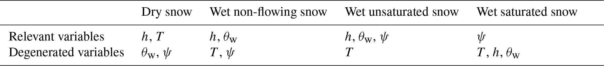
2.5 Choosing primary variables in the presence of regime changes

A difficulty with the system presented in Eq. (13) (complemented with its material laws) is the presence of 4 distinct regimes, where parts of the equations behave differently and sometimes degenerate. The first regime corresponds to dry snow, when the temperature is below the freezing point. Here, the thermodynamical state of snow can be characterized by either its temperature or its energy content (the two being related by the thermal capacity). On the contrary, the LWC and the matric potential cannot be used to describe the state of snow, as they assume constant, degenerate, values. In the second regime, the snow is at its fusion point, but the LWC remains below its retention value. Here, the snow can be characterized by its energy content or its LWC, but not by its temperature nor its matric potential. The third regime corresponds to the classical unsaturated Richards' case, where the LWC is above the retention point. Here, the snow can be characterized by its energy content, its LWC, or its matric potential, but not by the temperature. The fourth regime corresponds to the water-saturated regime. Here, the snow can only be characterized by its matric potential. This regime corresponds to the saturated regime of Richards' equation. A summary of the different regimes and the variables that can be used to characterize them is given in the Table 1. As seen, there is no natural variable that can be used to describe the thermodynamical state of snow over the 4 different regimes. While the energy content could be used to characterize snow in regimes 1, 2, and 3, it degenerates in regime 4. Similarly, while the matric potential is a good candidate to describe regimes 3 and 4 (as usually done when numerically solving Richards' equation; Celia et al., 1990; Farthing and Ogden, 2017), it fails in regime 1 and 2.

Table 1 Summary of the various regimes encountered in snow. For each regime, the relevant variables that can be used to characterize snow are given, as well as the degenerated variables that cannot be used to characterize snow. In all cases, the ice volume fraction ϕ_i is also needed as a second variable.

To circumvent this issue, we rely on a variable switch technique by parametrization (Brenner and Cancès, 2017), through the use of a fictitious variable meant to behave as the energy content in the first three regimes and as the water matric potential in the last one (Bassetto et al., 2021, 2022). For this, we introduce a new variable χ (expressed in J m⁻³) used to parameterize the {h,ψ} graph. Specifically, we choose χ such that

$$\begin{array}{}\text{(14)}& {\displaystyle }h(\mathit{\chi },{\mathit{\varphi }}_{\mathrm{i}})=\left\{\begin{array}{ll}\mathit{\chi }& \text{if }\mathit{\chi }<{\mathit{\theta }}_{\mathrm{s}}\left({\mathit{\varphi }}_{\mathrm{i}}\right){\mathit{\rho }}_{\mathrm{w}}{L}_{\text{fus}}\\ {\mathit{\theta }}_{\mathrm{s}}\left({\mathit{\varphi }}_{\mathrm{i}}\right){\mathit{\rho }}_{\mathrm{w}}{L}_{\text{fus}}& \text{otherwise}\end{array}\right.\text{(15)}& {\displaystyle }\mathit{\psi }(\mathit{\chi },{\mathit{\varphi }}_{\mathrm{i}})=\left\{\begin{array}{ll}\mathit{\psi }\left({\mathit{\theta }}_{\mathrm{w}}\right(\mathit{\chi },{\mathit{\varphi }}_{\mathrm{i}}\left)\right)& \text{if }\mathit{\chi }<{\mathit{\theta }}_{\mathrm{s}}\left({\mathit{\varphi }}_{\mathrm{i}}\right){\mathit{\rho }}_{\mathrm{w}}{L}_{\text{fus}}\\ \frac{\mathit{\chi }-{\mathit{\theta }}_{\mathrm{s}}\left({\mathit{\varphi }}_{\mathrm{i}}\right){\mathit{\rho }}_{\mathrm{w}}{L}_{\text{fus}}}{\mathit{\beta }}& \text{otherwise}\end{array}\right.\end{array}$$

where β is an arbitrary constant, introduced to respect the unit homogeneity of Eq. (15), and where the dependence of ϕ_i has also been made explicit. Thanks to this variable χ, we are now able to characterize the energy content and matric potential of snow in all regimes, and from it to derive the values of all other relevant quantities for snow (θ_w, T, k_r, etc.).

Once parameterized with χ our system of equation becomes

$$\begin{array}{}\text{(16)}& \left\{\begin{array}{ll}{\partial }_{t}h(\mathit{\chi },{\mathit{\varphi }}_{\mathrm{i}})-\mathrm{\nabla }\cdot \left(\mathit{\lambda }\mathrm{\nabla }T\right(\mathit{\chi },{\mathit{\varphi }}_{\mathrm{i}}\left)\right)& \\ +{\mathit{\rho }}_{\mathrm{w}}{L}_{\text{fus}}\mathrm{\nabla }\cdot \left(K^{\text{sat}}{k}_{\mathrm{r}}\right(\mathrm{\nabla }\mathit{\psi }(\mathit{\chi },{\mathit{\varphi }}_{\mathrm{i}})+\cos \mathit{\gamma }\left)\right)\\ -Q_{\text{abs}}=\mathrm{0}\\ {\mathit{\rho }}_{\mathrm{w}}{\partial }_t{\mathit{\theta }}_{\mathrm{w}}(\mathit{\chi },{\mathit{\varphi }}_{\mathrm{i}})+{\mathit{\rho }}_{\mathrm{i}}{\partial }_t{\mathit{\varphi }}_{\mathrm{i}}& \\ -{\mathit{\rho }}_{\mathrm{w}}\mathrm{\nabla }\cdot \left(K^{\text{sat}}{k}_{\mathrm{r}}\right(\mathrm{\nabla }\mathit{\psi }(\mathit{\chi },{\mathit{\varphi }}_{\mathrm{i}})+\cos \mathit{\gamma }\left)\right)=\mathrm{0}\end{array}\right.\end{array}$$

that can be solved searching for χ and ϕ_i. We have explicitly shown the dependency of h, T, ψ, and θ_w on both χ and ϕ_i, but one should keep in mind that the effective properties λ, K^sat, and k_r also depend on the value of χ and ϕ_i. With this set of equations, we now have a consistent description of the energy and mass budgets in snowpacks that naturally applies to both dry and wet snow.

3 Numerical implementations

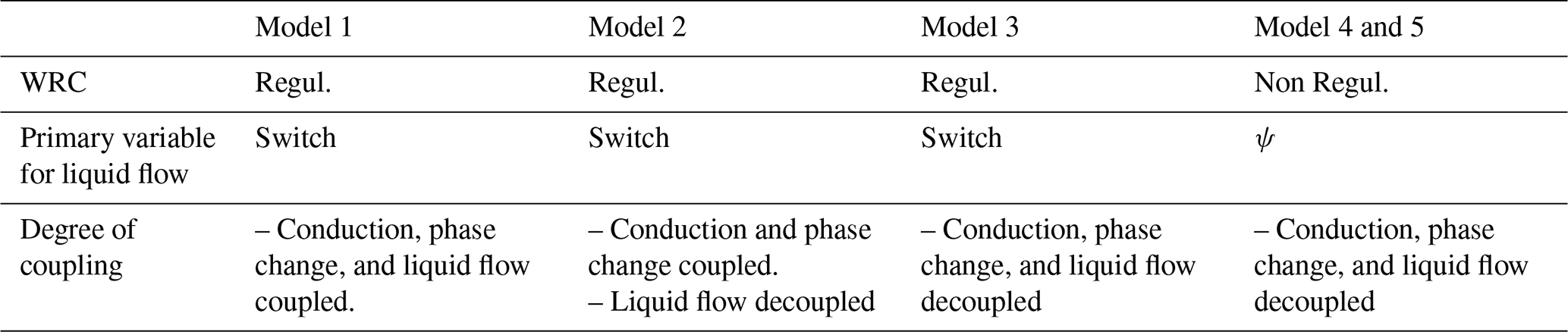
The goal of this section is to present and explore different numerical implementations of the energy and mass budgets in snow, in order to investigate the impacts of the implementation on the results and robustness of the models. We decided to focus this comparison on (i) the use of a regularized WRC with variable switching for matric flow, and (ii) the loosely or tightly-coupled nature of the implementation, where processes can either be solved sequentially (i.e. with operator-splitting) or concomitantly (i.e. with tight-coupling) (Steefel and McQuarrie, 1996; Keyes et al., 2013). By varying the regularization of the WRC and the degree of operator-splitting, we have implemented five snowpack toy-models. Below, we start by briefly presenting the common features shared by all implementations, and then discuss the concrete differences between them. These differences between the numerical implementations are summarized in Table 2.

Table 2 Description of different implemented toy-models based on (i) the regularization of the WRC, (ii) whether the primary variable is a switch (behaving as h in unsaturated snow and ψ in saturated snow) or ψ for solving the matric flow process, and (iii) the degree of couplings between thermodynamics processes.

3.1 A common core between all models

In order to be directly comparable, the models share portions of their numerical implementations. This includes compaction under mechanical stress (assuming a linear viscosity between stress and deformation and which is solved after the thermodynamics), the constitutive laws defining the material properties of snow, the spatial and temporal discretization, and the method for solving the resulting non-linear systems of equations.

3.1.1 Constitutive laws

To be fully closed, the equations of energy and mass conservation need to be complemented with constitutive laws, prescribing the material properties of the snow material. We assume the thermal conductivity λ of snow to follow Calonne et al. (2011) and the saturated hydraulic conductivity K^sat to follow Calonne et al. (2012). The WRC (Eq. 7) and the relative hydraulic conductivity (Eq. 9) require defining the parameters α and n. For this, we follow Yamaguchi et al. (2012). The residual LWC θ_r is taken as 0.02 (Yamaguchi et al., 2010; Wever et al., 2014; D'Amboise et al., 2017) and the saturated LWC θ_s as 1−ϕ_i (i.e. the total porosity). Finally, for the compaction of the snowpack under mechanical settling, we use the linear compactive viscosity of Vionnet et al. (2012), including its dependence on the LWC. The precise expressions for the constitutive laws are given in Appendix B.

3.1.2 Finite Volume discretization

To be numerically solved, the system of Eqs. (16) needs to be discretized in time and space. For the time discretization, we use a simple backward Euler time-stepping. This choice is motivated by the overall stability of the method, mitigating the appearance of overshoots and oscillations in the case of large-time steps (Butcher, 2008). For the spatial discretization, we use a finite volume scheme. Briefly, this numerical method relies on dividing the snowpack into N cells and performing energy and mass balances on each individual cell. In this framework, each cell is described by its average χ and ϕ_i values. The evolution of these average values is obtained by integrating the system of equations over the different cells, and applying the divergence theorem to transform the divergence operator into fluxes at the cells' boundaries.

To be mathematically closed, the heat and liquid water fluxes at the interface between two adjacent cells need to be reconstructed from the cells' averages. For the heat fluxes, this is done by computing the temperature gradient from one cell center to the other, and defining an interfacial thermal conductivity. As classically done in finite volume schemes, this interfacial thermal conductivity ${\mathit{\lambda }}^{k+\mathrm{1}/\mathrm{2}}$ (between cells k and k+1) is taken as some average of the thermal conductivities of the adjacent cells. In our case, we take it as the weighted harmonic average. This is consistent with the idea that the conductances corresponding to adjacent cells are placed in series. It notably ensures that the heat flux vanishes when the thermal conductivity of one of the two cells vanishes (Kadioglu et al., 2008).

For the computation of the liquid water flux, the gradient of the matric potential is also computed based on the average values in the cells and the center-to-center distance. For the computation of the interfacial hydraulic conductivity, we use the so-called upstream mobility formulation (Bassetto et al., 2021). In this framework, the hydraulic conductivity of the interface is split into the product of the saturated conductivity $K_{\text{sat}}^{k+\mathrm{1}/\mathrm{2}}$ and the relative conductivity $k_{\mathrm{r}}^{k+\mathrm{1}/\mathrm{2}}$. As with the thermal conductivity, the interfacial saturated conductivity is taken as the harmonic average of the saturated conductivities of the neighboring cells. This ensures that the liquid water flux vanishes when one the of the cells is impermeable. The interfacial relative conductivity $k_{\mathrm{r}}^{k+\mathrm{1}/\mathrm{2}}$ between cell k and k+1 is taken as the upstream value, i.e.

$$\begin{array}{}\text{(17)}& k_{\mathrm{r}}^{k+\mathrm{1}/\mathrm{2}}=\left\{\begin{array}{ll}{k}_{\mathrm{r}}^k& \text{if}{\mathit{\psi }}^k>{\mathit{\psi }}^{k+\mathrm{1}}+\cos \mathit{\gamma }{d}^{k+\mathrm{1}/\mathrm{2}}\\ k_{\mathrm{r}}^{k+\mathrm{1}}& \text{otherwise}\end{array}\right.\end{array}$$

where $d^{k+\mathrm{1}/\mathrm{2}}$ is the distance between the neighboring cell centers and $\cos \mathit{\gamma }{d}^{k+\mathrm{1}/\mathrm{2}}$ thus is the vertical distance between the cell centers. With this upstream choice, the numerical scheme becomes monotonic (in the sense of Eq. 3.18 of Bassetto et al., 2021). This property is notably beneficial for the convergence of the Newton (or other iterative) method, when solving the resulting non-linear system of equations.

3.1.3 Truncated Newton method with adaptive time-stepping

The systems of equations to be numerically solved in the different models are non-linear and require an iterative scheme. For that, we rely on a Newton method, with a stopping criterion when the iterated estimations is close enough to the solution. In two of the implementations that will be presented below (denoted models 4 and 5), this criterion is complemented with a criterion on mass conservation, as these numerical schemes are not naturally mass-conservative. While the Newton algorithm provides a relatively fast convergence when the starting estimation is close to the solution, it is not a globally convergent algorithm. In other words, it is possible for the algorithm to produce diverging iterations or even to produce iterations that oscillate without converging to the solution. To improve its convergence performance, we implemented two strategies. First, as usually done with Richards' equation we use an adaptive time-step. In the case where the algorithm fails to converge after a given number of iterations, the algorithm is rewound to the start of the time-step and its value halved. By default, we set the maximum number of iterations to 25. In the rest of the article, we thus make the difference between the so-called “default timestep”, corresponding to the timestep that is ideally used if no convergence problems are encountered, and the “adaptive timestep”, that is effectively used to solve the nonlinear equations involving matric flow. Secondly, we use the so-called truncation method when a transition from one regime to another occurs (Bassetto et al., 2020). Indeed, the transitions between regimes are corner points, characterized by discontinuities in the derivatives. Using the derivative computed on one side of a corner point to derive the evolution of the estimate in the other side is therefore problematic and can lead to overshoots, impeding the convergence towards the solution. To avoid this problem, each time a transition from one regime to another occurs in a cell of the snowpack, χ is set back in the vicinity of the corner point. In practice, χ is placed at a small ϵ value before or after the corner point, in order to fall in the good regime. We set this value of ϵ to be 10⁻⁵ J m⁻³. Finally, we note that for solving Richards' equation the SNOWPACK (Wever et al., 2014) and Crocus (D'Amboise et al., 2017) models decided to follow a modified Picard method (Celia et al., 1990), where the contribution of the change in hydraulic conductivity in the Jacobian is not taken into account. As a test, we also run some simulations using the modified Picard rather than the Newton method. As this did not modify the results of the article (not shown), it will not be further discussed.

3.2 Differences between the five different numerical implementations

3.3 Model 1: Fully coupled with a regularized WRC

For the first model, we use the regularized WRC and solve the energy and mass budgets in a tightly-coupled manner, that is to say that the system of Eq. (16) is solved concomitantly for both χ and ϕ_i. In this version, there is therefore no degree of operator-splitting when solving the thermodynamical state of the snowpack.

3.4 Model 2: Partially coupled with a regularize WRC

While the numerical implementation of model 1 appears to be the most consistent, it results in a large non-linear system that can be numerically expensive to solve. As a compromise, some degree of operator-splitting (i.e. sequentiallity) between processes can be introduced. For model 2, we thus used the regularized WRC with a decoupling of the computation of the energy and liquid water budgets from that of the ice budget. The motivation behind it is that the timescale for the evolution of the density is usually longer (of the order of a day, unless in case of abrupt melting) than that of the energy and LWC evolution (of the order of an hour or less). Concretely, in Eq. (16) we thus first solve the evolution of χ (assuming a fixed ϕ_i). Then, we find the evolution of ϕ_i by closing the mass budget.

3.5 Model 3: Full operator-splitting with a regularized WRC

Keeping with the idea of using operator-splitting to reduce the numerical cost and complexity of the model, the third implementation is based on a decoupling of the energy, liquid water, and ice budgets solutions. Specifically, we first evolve χ under the process of heat conduction and phase changes only. We then evolve χ again, this time under the process of matric liquid water flow. Finally, ϕ_i is updated by re-applying phase transition and closing the mass budget.

3.6 Model 4 and 5: Full operator-splitting without a regularized WRC

The last two models are meant to emulate the techniques used so far in snow models to handle the degeneracy of the retention curve in dry snow. Specifically, model 4 is based on the SNOWPACK implementation (Wever et al., 2014) and model 5 on the Crocus implementation (D'Amboise et al., 2017). The specificities of the implementation are given in Appendix C, but we recall that both techniques are based on the idea of introducing a small amount of liquid water in cold snow, shifting the residual liquid water content value below it, and using ψ as the primary variable. Moreover, these models rely on a decoupled solution of the thermodynamical processes.

4 Numerical tests

The goal of this section is to build simple synthetic examples, meant to represent different situations in which liquid water percolation might occur in snowpacks, and to investigate the differences in behavior between the various implementations.

Table 3 Description of three different test cases considered in this article, with their durations and external forcings.

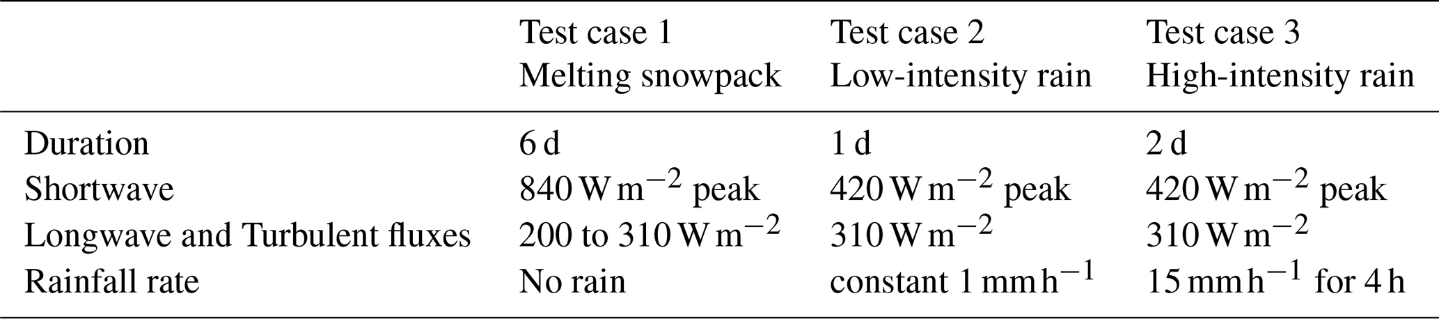
4.1 Test case 1: Melting snowpack

The first test case is meant to represent the situation of melting snowpack, releasing liquid water near the surface that then percolates downward. For the initialization of the snowpack, we rely on a simulation performed with the Crocus snowpack (Vionnet et al., 2012). This yields a realistic stratigraphy, with thinner cells near the surface in order to better capture the generally steep gradients of density, temperature, and liquid water content near the surface. For the initial state of the simulation, the initial temperature was decreased compared to the Crocus output in order to obtain a cold and dry snowpack near its peak snow water equivalent. This defines the ice volume fraction, temperature, and specific surface area at the start of our simulations. Note that the specific surface area is needed as it plays a role in the hydraulic properties of the snowpack (Calonne et al., 2012; Yamaguchi et al., 2012). However, as we did not implement metamorphism laws in our toy model, the specific surface area is simply kept constant during the simulation.

For the top boundary conditions, we impose an incoming diurnal energy flux at the surface of the snowpack (oscillating between 310 W m⁻² at noon and 200 W m⁻² at night), encapsulating the effect of incoming longwave radiation and turbulent heat fluxes. We also impose diurnal shortwave radiation (peaking at 840 W m⁻² at noon and vanishing at night) that penetrates within the snowpack (with an albedo of 0.7 and an e-folding depth of 5 cm; Libois et al., 2013). No liquid, nor solid, precipitation is considered in this test case. As the bottom boundary condition, we impose a constant heat flux of 10 W m⁻², emulating the heat flux received from a warm ground below, and a free-drainage condition for the liquid water flux. For each model, simulations are run for 6 d, so that water percolates to the bottom of snowpack. Default timesteps vary between 112 and 7200 s (we recall that because of the adaptive timestep strategy, the actual timestep used for some process might be shorter than the prescribed default value).

4.2 Test case 2: Water infiltration under low-intensity rain

This second test case is meant to represent the slow infiltration of rain under a long but low-intensity event. The initialization is the same as in case 1, based on the output of the same Crocus simulation, but with a higher temperature in order to have a snowpack close to its melting point. For the top boundary condition, we impose a constant surface energy flux of 310 W m⁻², a shortwave radiation flux peaking at 420 W m⁻² at noon (lower than in the first test case to represent cloudiness), and a constant rain flux of 1 mm h⁻¹ lasting the whole simulation. For the bottom boundary condition, we use the same conditions as in the test case 1 (constant heat flux and free-drainage). Simulations were performed with each model for 1 d, in order for shallow infiltration to occur. Default timesteps range from 112 to 7200 s.

4.3 Test case 3: Water infiltration under high-intensity rain

The third test case represents the case of a short but high-intensity rain event. The initialization is also based on a Crocus simulation, with a temperature field intermediate between test case 1 and 2. The boundary conditions are taken as in test case 2, except for the incoming rain flux that is now 15 mm h⁻¹ and lasts for 4 h. This results in an abrupt input of liquid water in the snowpack, rapidly percolating downward. Simulations were run for about 2 d, long enough for deep percolation to occur. Default timesteps range from 112 to 7200 s.

The initial conditions for the density, SSA, and temperature are displayed in Fig. 2. For all three test cases, reference simulations were performed with the fully coupled model (model 1) and a timestep of 1 s. The resulting LWC profiles over time are displayed in Fig. 3. As seen in the figure, the first test case shows diurnal surface melt with liquid water infiltrating deeper in the snowpack days after days. Note that a significant amount of liquid water is retained around the 20 cm horizon. This coincides with an abrupt drop in the snow SSA, which acts as a capillary barrier. In the second test case, surface melt is less pronounced due to the lower input radiative fluxes. The constant rain input produces a steady percolation of the liquid water that reaches about the middle of the snowpack after a day. In the last test case, the abrupt rain input results in a fast movement of the percolation front through almost the whole snowpack. As in the first test case, a significant amount of liquid water is retained around the 20 cm horizon. In these three cases, liquid water is produced directly at the bottom of the snowpack in response to the 10 W m⁻² heat flux from the warm ground. In the absence of such heat flux, the bottom of the snowpack would remain dry until liquid water percolates through the whole snowpack. Finally, we note that using model 1 as a benchmark is not neutral, as it places this model in a specific position compared to the others. This choice was made as we expect its physics to be the most cleanly defined (without diverging WRC and artificial displacement of the residual LWC to circumvent this divergence) and that the use of operator-splitting is known to introduce errors (Keyes et al., 2013; Connors et al., 2014)

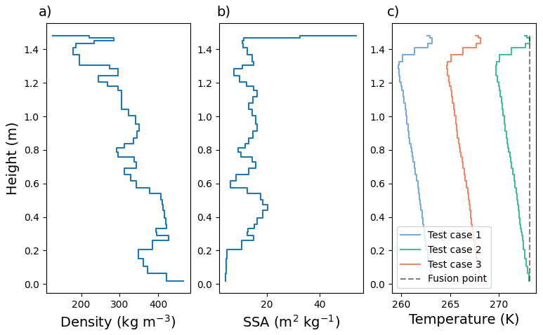
Figure 2 Initial conditions of the snowpack used in the simulation, in terms of density (panel a), SSA (panel b), and temperatures (panel c). Note that the initial temperatures are lower in test cases 1 and 3 in order to simulate liquid water infiltration withing a colder snowpack.

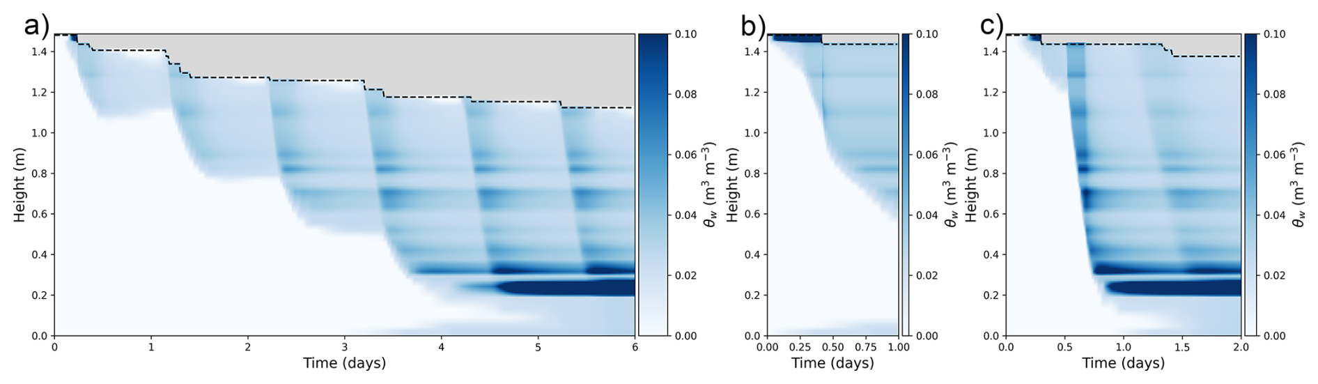
Figure 3 Results of the reference simulations for the three investigated test cases: (a) surface melting with a deep infiltration of surface melt, (b) a low-intensity rain with limited infiltration, (c) a high-intensity rain event with a fast and deep water infiltration.

5 Results and discussion

5.1 Robustness and numerical cost

The first difference in behavior between the different implementations is their respective numerical cost, i.e. the computation time required to perform a given simulation. In the presence of an adaptive timestep, required to accommodate the strong non-linearity of the liquid matric flow and of the WRC, we observed that the numerical cost of the models is, at first order, controlled by the ability of the models to stick to large adaptive timesteps. Figure 4 displays the adaptive timesteps required by the models in the three test cases presented above. While the models using a regularized retention curve with a variable switch (models 1, 2, and 3) are able to maintain a timestep of around 1 h for most of the simulations, models 4 and 5 require the adaptive timestep to regularly drop, sometimes below 10 s. In the end, models 4 and 5 require about one order of magnitude more steps to perform the same simulation, resulting in significantly increased numerical cost and computation time. For instance, in the case of the test case 3 with a default timestep of 3600 s, models 4 and 5 require a computation time of about 500 s, while models 1, 2, and 3 require about 130, 25, and 45 s, respectively. Note that these numbers should only be interpreted qualitatively to assess numerical complexity, as the precise computation time is also influenced by factors that we did not control for (such as the level of code optimization or memory-caching). Therefore, the use of a regularized WRC with a variable switch appears as a very favorable practice to increase the robustness of the numerical scheme and to decrease its numerical cost by accommodating larger timesteps. Our understanding of this behavior is that the combination of regularized WRC and not using the matric potential as the primary variable near the retention point hinders the presence of abrupt, and nonlinear, variations of the numerical solution, thus making the problem easier to solve. To the contrary, using the matric potential as the primary variable is known to be inefficient for low LWC materials and to require timesteps that are much smaller than the actual timescale of liquid water transport (Forsyth et al., 1995; Sadegh Zadeh, 2011).

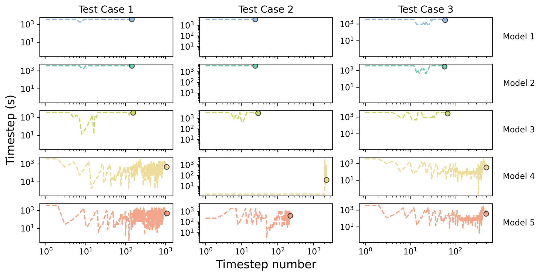
Figure 4 Adaptive timesteps required to simulate matric flow in each test case (columns) and for each model implementation (rows). The default value for the timestep is set to 3600 s. In each plot, the marker marks the total number of timesteps required and the average timestep size.

Focusing on models 1, 2, and 3 in Fig. 4, it appears that these three implementations require very similar timesteps, apart from a notable drop for model 3 in the first and second test case. Their differences in numerical cost should be controlled by the complexity of the assembly and solving of the matrix-form of the equations. According to our numerical test cases, models 2 and 3 have about the same numerical cost, while our implementation of model 1 requires a longer computational time. This is to be expected, as model 1 requires the largest matrix to be assembled and solved (2N×2N), while the other models handle smaller matrices (N×N). However, we also note that a large portion of the up-cost of model 1 comes from the computation of derivatives with respect to ϕ_i for the assembly of the Jacobian. In our implementation, computing these derivatives comes with a high cost, as we rely on generic automatic differentiation without any attempt at optimization. If these derivatives with respect to ϕ_i are ignored (thus transforming the scheme from a true Newton to a form of modified Picard method), the numerical solving of the coupled system of Eqs. (16) can be made more efficient. For instance, in the aforementioned test case 3 with a default timestep of 3600 s, the computational time can be lowered from 130 to about 50 s, i.e. in the same range as models 2 or 3.

5.2 Error-level and timestep convergence

Besides their numerical cost, the different implementations also yield different levels of error when compared to the reference simulations. While the error level generally tends to decrease with shorter timesteps, not all models perform the same for decreasing timesteps. Here, we thus investigate the degree error of each model, for default timesteps ranging from 7200 to 112 s. For that, we compute the Root Mean Square Difference (RMSD) between the models' outputs and the reference simulations. Figure 5 display the RMSDs in LWC and temperature for the three test cases as a function of the default timestep. Note that because of the presence of an adaptive timestep for solving liquid water percolation, the value of the default timestep should be interpreted with caution in Fig. 5. Indeed, as models 4 and 5 (and 3 to some degree) require small adaptive timesteps, their solving of liquid water percolation actually occurs with a timestep much lower than the default value. This gives them an advantage in terms of RMSD, as errors stemming from the temporal discretization of Richards’ equation are reduced in the process. Also, the RMSD is computed over the whole snowpack, while errors tend to be spatially located near the percolation front. Therefore, the RMSD value is smaller, typically by an order of magnitude, than the errors occurring at the percolation front. As expected, the overall trend is a decrease of the RMSDs with small timesteps. However, while the unregularized models 4 and 5 perform similarly as the other models with large default timesteps, they do not show a clear decrease of error at smaller timesteps. Our understanding is that the strategy of modifying the residual LWC based at the start of each timestep impacts the physics and changes the solution to which the models converge with small timesteps. This results in a plateau or even an increase of the associated RMSDs in Fig. 5. However, it further appears that model 3 does not show a clear convergence for vanishing timesteps as well, despite having in principle the same physics as model 2 and 3. This is visible in the tendency of the RMSD model 3 to plateau for timesteps below 225 s. After investigation, we found that model 3 actually diverges away from the benchmark solution for very small timesteps (of the order of the second). The same behavior for very small timesteps was seen for models 4 and 5 as well. This is puzzling as it suggests that either (i) models 3, 4, and 5 require timesteps well below 1 s to reach convergence, or that (ii) they do not have a converging solution with vanishing timesteps. Unfortunately, due to high numerical cost, we were not able to run the models well below the 1 s timestep to further explore this behavior. Concerning the regularized models (1, 2, and 3), our results suggest that model 1 consistently yields the lowest RMSDs for timesteps of 900 s and less. The comparison of the errors of models 2 and 3 for timesteps between 112 and 900 s depends on the specific test case and the variable of interest, with no clear advantage of one over the other. We note that under some circumstances (e.g. test case 2 and timestep of 900 s), one model can appear better in one metric (e.g. LWC RMSD) while it is outperformed in another metric (e.g. temperature RMSD).

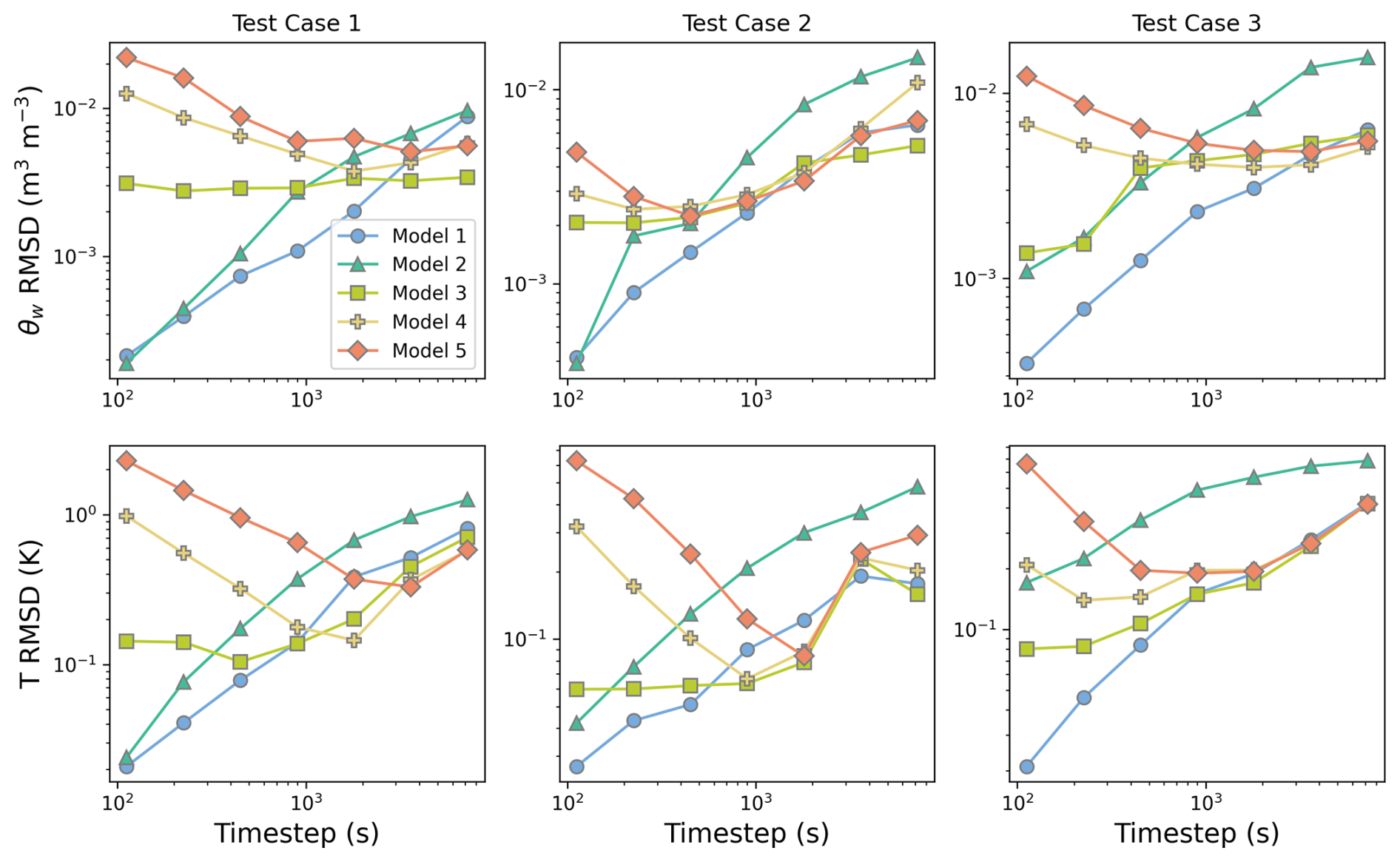
Figure 5 Root Mean Squared Difference in LWC and temperature between the models and a reference simulation as a function of the default timestep size.

5.3 Is full-coupling benificial?

As seen above, the use of a tightly-coupled solution in numerical models usually provides a slightly better precision and a better robustness (Keyes et al., 2013; Brondex et al., 2023), at the expense of a more complex numerical solution. Indeed, by ensuring physical consistency between the different variables, tightly-coupled solutions are known to prevent overshooting, which could develop into numerical oscillations or even divergence (Brondex et al., 2023). One of the motivation behind the investigation of the impact of operator-splitting on the numerical solution of the energy and mass budgets with liquid water matric flow was thus to examine whether a tightly-coupled solution was warranted in this case. To our surprise, the problem of heat conduction, liquid matric flow, and phase changes, appears to be quite robust to operator splitting. Indeed, even in the case of a quite large timestep of 4 h, we did not observe any clear sign of numerical instabilities or very large overshoots in the models using operator-splitting. Our understanding is that this overall insensibility to operator-splitting comes from the nature of the involved processes, which do not play in the same regimes. Indeed, the process of heat conduction only occurs in dry snow, the process of matric flow in wet snow, and the process of phase change at the wet-dry interface. The possibility of interaction between processes thus remains limited and the large physical inconsistencies, that can be problematic with operator-splitting, did not emerge in most situations. However, as explained in Sect. 5.2, it appears that the models with phase changes decoupled from heat conduction and liquid percolation (i.e. models 3, 4, and 5) do not yield well-converged solution with timesteps of 1 s. While we were not able to precisely explain this behavior, the fact that it appears in models 3, 4 and, 5 might suggest that it is linked with the use of operator-splitting for phase changes. However, this point needs to be further investigated. Therefore, the standard practice of operator-splitting seems to be overall well-justified, at least with timesteps of the order of 900 s and when representing the interaction of matric flow with heat conduction and phase changes in snowpack models.

5.4 Inclusion of other physical mechanisms

In this article, we considered the coupled mechanisms of heat conduction, matric liquid water percolation, and liquid-solid phase changes. While we focused on these mechanisms, as they can be found in all snowpack models (with more or less degrees of complexity), other thermodynamical mechanisms could be included as well. This is for instance the case of water vapor diffusion and vapor phase changes. To the best of our understanding, vapor-related mechanisms could be easily added to the systems of the thermodynamical equations governing snowpacks. For that, one would need to (i) introduce a new partial differential equation governing the mass balance of water vapor, (ii) introduce a water vapor component in the energy balance equation, and (iii) close the system by prescribing the phase change term for the gas phase (or assuming water vapor thermodynamical equilibrium with the other phases) and parametrizing the diffusivity of vapor. This could be done based on works of Calonne et al. (2014), Jafari et al. (2020), Brondex et al. (2023), and Bouvet et al. (2024). Similarly, an important mechanism relating to the transport of liquid water in snowpacks is the process of preferential (i.e. non-matric) flow (Schneebeli, 1995; Yamaguchi et al., 2018). While the exact mechanisms, and therefore description, of preferential flow in snowpacks remain unclear at this point (Hirashima et al., 2014, 2019; Moure et al., 2023), the presence of fast flowing, and out-of-equilibrium with the rest of the snow layer, liquid water appears as a prerequisite for the formation of internal horizontal ice layers. In this picture, the preferential flow transports liquid water through cold snow layers down to a capillary barrier, where the liquid water can then horizontally spread and refreeze as a horizontal crust (Quéno et al., 2020). This is illustrated by the close relation between refrozen preferential paths (i.e. ice columns) and internal horizontal crusts, for instance illustrated in picture #58 of Fierz et al. (2009). As percolation chimneys are likely to play a key role for preferential flow, the use of a so-called dual-porosity/dual-permeability model (e.g. Vogel et al., 2000; Lewandowska et al., 2004) has notably been proposed to take into account preferential flow in the SNOWPACK model (Wever et al., 2016; Quéno et al., 2020). As preferential flow shares many similarities with matric flow (being essentially a faster version), the governing equations are subjected to the same degenerate behaviors in the case of a dry or a fully-saturated medium. Therefore, the techniques explored in this article, namely the regularization of the WRC to handle dry media with the use of a switch variable, could also benefit the numerical implementation of preferential flow. Moreover, as preferential flow is a fast and out-of-equilibrium process, it can introduce stiffness in the equations governing snowpacks (Fazio, 2001), potentially resulting in overshoots and oscillations when using operator splitting with a large timestep (Brondex et al., 2023; Fourteau et al., 2024). As discussed above, the derivation of a fully-consistent system of equations, that applies from dry to water-saturated snow, enables a tightly-coupled numerical solution, which could be key to handle stiff and fast systems of equations (Keyes et al., 2013).

6 Conclusions

This article focuses on the numerical implementation of matric water flow and its interaction with other physical processes in snowpack models using Richards' equation. While the use of Richards' equation can improve the representation of water flow, its complexity and numerical cost can sometimes hinder widespread adoption. To overcome this issue, we explored a new numerical implementation of Richards' equation. We started by recalling the governing equations of energy and mass conservation in snowpacks that govern the evolution of the snow material both in dry and wet zones. However, for these equations to be directly applicable for both dry and wet snow, it is necessary to provide an expression of the liquid water flow that also applies in dry snow (where simply no flow is expected). For this, we regularized the water retention curve in order to avoid the divergence of the matric potential as the snow material dries. Another issue with the concomitant and consistent representation of a whole snowpack is that dry and wet snow are not described by the same thermodynamical variables, as dry snow is described in terms of temperature/energy while wet snow is rather described in terms of liquid water content/matric potential. To seamlessly handle this change in the physical variables characterizing the snow material, we introduced a variable switch technique implemented thanks to the introduction of a fictitious variable building on the idea introduced in Brenner and Cancès (2017). This defines a single thermodynamical variable to describe all states of snow, from dry to water-saturated. Eventually, we thus obtained a consistent system of two equations (energy and mass conservation) governing the evolution of snowpacks and which allows a unified treatment of dry and wet snow.

To compare the behavior and performance of this new description, we have implemented five toy snowpack models. This includes three models, all using a regularized WRC with a variable switch but relying on various degrees of operator splitting during the solution, as well as two models based on the treatment of Richards' equation in the SNOWPACK and Crocus snow models (i.e. using a non-regularized retention curve). Based on three test cases, representing various situations of snowpack humidification, we observe that the use of a regularized WRC with variable switch significantly increases the robustness of the numerical implementation, which can run with timesteps of 15 min and above without the need for a shorter internal timestep (although using large timesteps naturally results in a degradation of the simulations' accuracy), while the non-regularized models require shorter timesteps to handle liquid water percolation. On the other hand, the possibility of a fully tightly-coupled implementation seems to have a smaller impact compared to an operator-splitting implementation, both in terms of stability and timestep sensitivity. While this article focused on matric liquid flow, we believe that the methodology put forward, namely the use of regularized laws, variable switch, and physically consistent description of the various thermodynamical states of snow, could also be useful for the description of preferential flow. Indeed, as preferential flow is usually modeled as a faster version of matric flow, the ability of regularized models to nonetheless handle relatively large timesteps could prove crucial to limit their numerical cost.

Appendix A: Ice-Water thermodynamics equilibrium in snow

In this section, we briefly discuss the relaxation of the thermodynamics equilibrium assumption between the ice and water phases in snow. This appendix is largely based on the recent work of Moure et al. (2023). If we assume that the ice and liquid water are out-of-equilibrium, it is necessary to distinguish between the ice temperature and the liquid water temperature. It is thus no-longer possible to write a single energy-equation, as in Eq. (13). Similarly, we also need to distinguish between the solid and liquid mass budgets. The out-of-equilibrium ice and liquid water system is now described by T_i, T_w, m_i, and m_w (the ice and liquid temperatures and the ice and liquid mass content, expressed in kg m⁻³) and the four equations provided by Moure et al. (2023)

$$\begin{array}{}\text{(A1)}& \left\{\begin{array}{l}{\partial }_t\left(c_{\mathrm{i}}{m}_{\mathrm{i}}{T}_{\mathrm{i}}\right)+\mathrm{\nabla }\cdot {\mathit{F}}_{u,\mathrm{i}}=W_{\text{SSA}}\frac{{\mathit{\lambda }}_{\mathrm{i}}}{r_{\mathrm{i}}}(T_{\text{int}}-T_{\mathrm{i}})\\ {\partial }_t\left(c_{\mathrm{w}}{m}_{\mathrm{w}}{T}_{\mathrm{w}}\right)+\mathrm{\nabla }\cdot \left({\mathit{F}}_{\mathrm{w}}{c}_{\mathrm{w}}{T}_{\mathrm{w}}\right)\\ +\mathrm{\nabla }\cdot {\mathit{F}}_{u,\mathrm{w}}=W_{\text{SSA}}\frac{{\mathit{\lambda }}_{\mathrm{w}}}{r_{\mathrm{w}}}(T_{\text{int}}-T_{\mathrm{w}})\\ {\partial }_t{m}_{\mathrm{i}}=-{\mathit{\rho }}_{\mathrm{i}}{R}_m{W}_{\text{SSA}}(T_{\text{int}}-T_{\mathrm{0}})\\ {\partial }_t{m}_{\mathrm{w}}+\mathrm{\nabla }\cdot {\mathit{F}}_{\mathrm{w}}={\mathit{\rho }}_{\mathrm{i}}{R}_m{W}_{\text{SSA}}(T_{\text{int}}-T_{\mathrm{0}})\end{array}\right.\end{array}$$

where F_u,i, F_u,w, and F_w are heat conduction fluxes in the ice, in the water, and the water flux, respectively, $R_m=\frac{c_{\mathrm{w}}}{\mathit{\beta }{L}_{\text{fus}}}$ (with β the kinetic attachment coefficient for ice growth from liquid water and c_w the thermal capacity of liquid water), W_SSA is the wet surface area, T_int the temperature ice-liquid water interface, λ_i and λ_w are the ice and liquid water thermal conductivities, and r_i and r_w two microstructural parameters estimated to be 0.06 d_i and 0.081 d_i, respectively (with d_i the diameter of the grain in the snow microstructure; Moure et al., 2023). The temperature T_int is given as a linear combination of the ice, water, and melting temperature

$$\begin{array}{}\text{(A2)}& \begin{array}{rl}{T}_{\text{int}}& ={\displaystyle \frac{\frac{c_{\mathrm{w}}{\mathit{\rho }}_{\mathrm{w}}}{\mathit{\beta }}{T}_{\mathrm{0}}+\frac{{\mathit{\lambda }}_{\mathrm{i}}}{r_{\mathrm{i}}}{T}_{\mathrm{i}}+\frac{{\mathit{\lambda }}_{\mathrm{w}}}{r_{\mathrm{w}}}{T}_{\mathrm{w}}}{\frac{c_{\mathrm{w}}{\mathit{\rho }}_{\mathrm{w}}}{\mathit{\beta }}+\frac{{\mathit{\lambda }}_{\mathrm{i}}}{r_{\mathrm{i}}}+\frac{{\mathit{\lambda }}_{\mathrm{w}}}{r_{\mathrm{w}}}}}\\ & =b_{\mathrm{0}}{T}_{\mathrm{0}}+b_{\mathrm{i}}{T}_{\mathrm{i}}+b_{\mathrm{w}}{T}_{\mathrm{w}}.\end{array}\end{array}$$

In this system of equations, the temperature of the ice-liquid interface governs the chemical equilibrium. Melting occurs if T_int>T₀, freezing occurs if T_int<T₀, and local equilibrium is achieved when T_int=T₀.

A difficulty in this equation is relating W_SSA to the actual specific surface area. Here, we follow Moure et al. (2023) and assume that W_SSA scales linearly with the saturation degree S (i.e. liquid water filling 50 % of the porosity would wet 50 % of the interfaces). However, we note that as the liquid water is the wetting phase in snow, it preferentially covers the ice surface, and the interface rapidly gets wet when liquid water is present. Therefore, the assumption that the wet SSA scales linearly with the saturation degree is likely an underestimation, which slows down the relaxation towards thermodynamics equilibrium in snow. To estimate the timescale of relaxation, we have implemented a simple model simulating relaxation towards local equilibrium (ignoring spatial fluxes for simplicity in the system of Eqs. A1). Figure A1 shows the evolution of the temperatures of the ice, the liquid water, and the interface, with $T_{\mathrm{i}}=\mathrm{273.15}=T_{\mathrm{0}}$ K, T_w=274.15 K, m_i=275 kg m⁻³, m_w=100 kg m⁻³, and a SSA of 2 m² kg⁻¹ as initial conditions. This illustrates that starting from a situation of non-equilibrium, thermodynamical equilibrium is achieved within about 20 ms. As this timescale of relaxation is much shorter than the timescale of evolution of the snowpack, the assumption of thermodynamical equilibrium between the ice and liquid water appears justified.

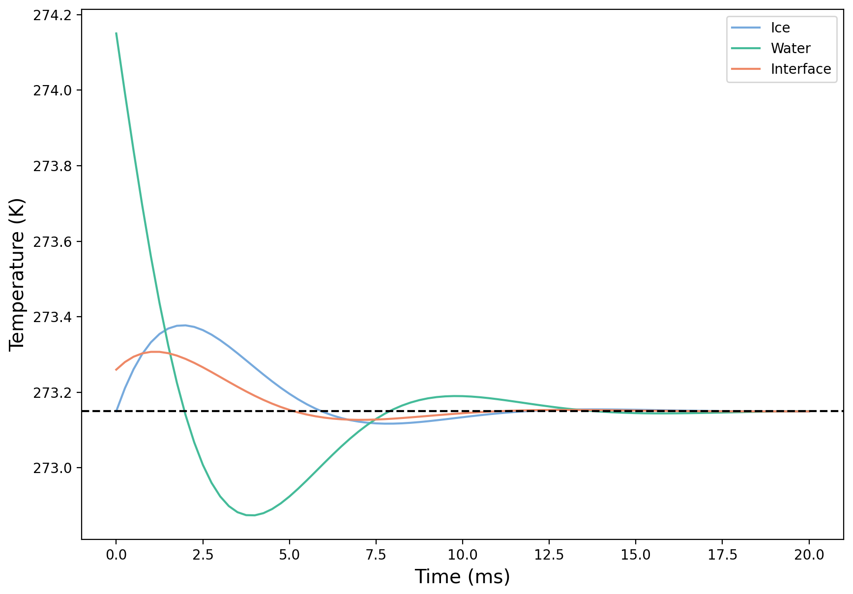
Figure A1 Evolution of ice, liquid water, and interface temperatures towards equilibrium, starting from a non-equilibrium situation.

Appendix B: Constitutive laws

This appendix presents the constitutive laws chosen for the models. For the thermal conductivity (expressed in $\mathrm{W}{\mathrm{K}}^{-\mathrm{1}}{\mathrm{m}}^{-\mathrm{1}}$) we have

$$\begin{array}{}\text{(B1)}& \mathit{\lambda }=\mathrm{2.5}\times {\mathrm{10}}^{-\mathrm{6}}{\mathit{\varphi }}_{\mathrm{i}}{\mathit{\rho }}_{\mathrm{i}}-\mathrm{1.23}\times {\mathrm{10}}^{-\mathrm{4}}{\mathit{\varphi }}_{\mathrm{i}}{\mathit{\rho }}_{\mathrm{i}}+\mathrm{0.024}\end{array}$$

and for the saturated hydraulic conductivity (expressed in m s⁻¹)

$$\begin{array}{}\text{(B2)}& K^{\text{sat}}={\displaystyle \frac{g{\mathit{\rho }}_{\mathrm{w}}}{{\mathit{\mu }}_{\mathrm{w}}}}\mathrm{3}{r}_{\text{es}}^{\mathrm{2}}\exp (-\mathrm{0.0130}{\mathit{\varphi }}_{\mathrm{i}}{\mathit{\rho }}_{\mathrm{i}})\end{array}$$

where g=9.81 m s⁻² is the gravity acceleration, ρ_w is the density of liquid water and ${\mathit{\mu }}_{\mathrm{w}}=\mathrm{1.79}\times {\mathrm{10}}^{-\mathrm{3}}$ Pa s is the dynamic viscosity of water at 0 °C, and $r_{\text{es}}=\mathrm{3}/\left(\text{SSA}{\mathit{\rho }}_{\mathrm{i}}{\mathit{\varphi }}_{\mathrm{i}}\right)$ is the equivalent optical radius. For the α and n parameters, defining the van Genuchten WRC, we have

$$\begin{array}{}\text{(B3)}& \mathit{\alpha }=\mathrm{4.4}\times {\mathrm{10}}^{\mathrm{6}}{\left({\displaystyle \frac{{\mathit{\varphi }}_{\mathrm{i}}{\mathit{\rho }}_{\mathrm{i}}}{\mathrm{2}{r}_{\text{es}}}}\right)}^{-\mathrm{0.98}}\end{array}$$

and

$$\begin{array}{}\text{(B4)}& n=\mathrm{1}+\mathrm{2.7}\times {\mathrm{10}}^{-\mathrm{3}}{\left({\displaystyle \frac{{\mathit{\varphi }}_{\mathrm{i}}{\mathit{\rho }}_{\mathrm{i}}}{\mathrm{2}{r}_{\text{es}}}}\right)}^{\mathrm{0.61}}.\end{array}$$

Finally, for the compactive viscosity η (expressed in Pa s) we have

$$\begin{array}{}\text{(B5)}& \mathit{\eta }={\displaystyle \frac{\mathrm{3.05}\times {\mathrm{10}}^{-\mathrm{7}}}{\mathrm{1}+\mathrm{60}{\mathit{\theta }}_{\mathrm{w}}}}{\displaystyle \frac{{\mathit{\varphi }}_{\mathrm{i}}{\mathit{\rho }}_{\mathrm{i}}}{\mathrm{250}}}\exp \left(\mathrm{0.1}\right(T_{\mathrm{0}}-T)+\mathrm{0.023}{\mathit{\varphi }}_{\mathrm{i}}{\mathit{\rho }}_{\mathrm{i}}).\end{array}$$

Appendix C: Details on the implementation of models without WRC regularization

In this appendix, we briefly present the implemenations of models 4 and 5, which are based on the treatment of Richards' equation in the SNOWPACK (Wever et al., 2014) and Crocus (D'Amboise et al., 2017) models, respectively. Note, that even though our implementations are based on SNOWPACK and Crocus, they cannot be considered as strict copies. Rather, our implementations mimic how the treatment of Richards' equation in SNOWPACK and Crocus could be translated into other models.

C1 Model 4

The implementation of this model is based on the SNOWPACK implementation (Wever et al., 2014) and its publicly available source code (master branch, f89d8c17 commit; checked on 16 December 2024). As explained in the main part of the manuscript, we follow here a sequential scheme, where the process of heat conduction, surface energy fluxes, and phase changes are first solved (and liquid percolation treated in a second step). This yields a LWC field, potentially with wet zones that flows and dry zones where the WRC is undefined. This issue is circumvented in two steps: (i) a small amount of liquid water is introduced, to avoid fully-dry media and (ii) the residual point of the WRC is lowered-down such that the LWC lies on a defined part of the WRC. Concretely, to solve Richards' equation, at the beginning of each adaptive timestep:

1. We compute the residual LWC of the snow material ${\mathit{\theta }}_{\mathrm{r}}=\text{max}(\mathrm{0},\text{min}({\mathit{\theta }}_{\mathrm{w}}-{\mathit{\theta }}_{\text{acc}}/\mathrm{10},\mathrm{\text{max}}(\mathrm{0},\text{min}(\mathrm{0.02},\text{max}({\mathit{\theta }}_{\mathrm{r}}^{\text{prev}},\mathrm{0.75}{\mathit{\theta }}_{\mathrm{w}})\left)\right)\left)\right)$, with θ_w the LWC at the start of the timestep, ${\mathit{\theta }}_{\mathrm{r}}^{\text{prev}}$ the residual LWC used in the previous timestep, and θ_acc the error aimed for on θ_w during the non-linear iteration. This step defines a residual LWC that is positive, equals the default value of 0.02 when the snow LWC is above 0.027, and tends to 75 % of the LWC when it is below 0.027. This corresponds to the lines 395 to 397 in the vanGenuchten.cc source file of SNOWPACK.

2. We compute the matric potential of “dry” layers. For this, we compute the matric potential of layers if they were just above their residual points. We then compute the minimum (maximum in absolute value) of these matric potentials, and define it as the matric potential that “dry” layers should have. This corresponds to the lines 967 to 969 in the ReSolver1d.cc source file of SNOWPACK.

3. We compute the minimum required LWCs that need to be present in the snow layers to reach the “dry” matric potential. This corresponds to line 976 to 999 in the ReSolver1d.cc source file of SNOWPACK.

4. If needed, we increase the LWC of layers that fall below their minimum required LWCs (computed in step 3 above), and recompute the residual LWC as in step 1. In order to ensure mass conservation, this is done by taking mass from the ice. This corresponds to the lines 1017 to 1024 in the ReSolver1d.cc source file of SNOWPACK.

After this step, we obtain consistent fields of LWC and WRC for the whole snowpack. Richards' equation (liquid water conservation under matric flow) is solved using the matric potential as the primary potential. For consistency with the other toy-models, we use a Newton method for the non-linear iterations. As with the other models, the stopping criterion is based on the error when trying to close the PDE, with an additional criterion on mass conservation (as using the matric potential as the primary variable affects mass conservation, Celia et al., 1990).

C2 Model 5

Model 5 is based on the Crocus implementation of Richards' equation (D'Amboise et al., 2017) and its source code (damboise_dev branch, 67bda59d commit; checked on 16 December 2024). It follows the overall same strategy as model 4. The main difference relates to the definition of the residual LWC. Concretely, at the beginning of each (adaptive) timestep:

1. We compute the residual points of the snow material as ${\mathit{\theta }}_{\mathrm{r}}=\text{min}(\mathrm{0.02},\mathrm{0.75}{\mathit{\theta }}_{\mathrm{w}})$, with θ_w the LWC at the start of the timestep. This results in a residual LWC that equals the standard value of 0.02 in well-wet material (θ_w>0.027), and that can drop to zero in the case of fully-dry material. This corresponds to the lines 3417 in the snowcro.F90 source file of Crocus.

2. We compute the matric potential of “dry” layers. This corresponds to the minimum matric potential of the layers when they are at the so-called “pre-wetting” level (${\mathit{\theta }}_{\mathrm{w}}={\mathrm{10}}^{-\mathrm{5}}$; D'Amboise et al., 2017). This corresponds to the lines 3408 to 3438 in the snowcro.F90 source file of Crocus.

3. If the LWC of a cell is below the “pre-wetting” level, the LWC is increased so that the matric potential reach the “dry” matric potential. This is done without ensuring mass conservation.

4. The residual points are re-computed as in step 1.

After this step, liquid water matric flow is solved using the same strategy as in model 4.