The Community Fire Behavior model for coupled fire–atmosphere modeling: implementation in the Unified Forecast System

There is an increasing need for simulating the evolution of wildland fires. The realism of the simulation increases by accounting for feedbacks between the fire and the atmosphere. These coupled models combine a fire behavior model with a regional numerical weather prediction model and have been used for fire research during the last few decades. This is the case, for instance, for the widely adopted Weather Research and Forecasting model with fire extensions (WRF-Fire). Typically, the coupling includes specific code for the particular models being coupled such as interpolation procedures to exchange variables between the atmospheric grid to the fire grid, and vice versa. However, having a fire modeling framework that can be coupled to different atmospheric models is advantageous to foster collaborations and joint developments. With this aim, we have created, for the first time, a fire behavior model that can be connected to other atmospheric models without the need for developing specific low-level procedures for the particular atmospheric model being used. To this end, the fire behavior model, referred to as the Community Fire Behavior model (CFBM), makes use of the Earth System Modeling Framework (ESMF) library to communicate information between the fire and the atmosphere. More specifically, CFBM is available as a national unified operational prediction capability (NUOPC) component which allows for an agnostic coupling to atmospheric models and other Earth system components. CFBM closely follows WRF-Fire version 4.3.3 methods in its version 0.2.0 which allows us to verify the adequacy of our implementation. The CFBM can be also run offline using an existing WRF simulation to propagate the fires in what we refer to as the standalone model. Herein we describe CFBM and its implementation in the Unified Forecast System (UFS). Simulations of the Cameron Peak Fire performed with UFS and WRF-Fire are presented to compare results from both models in order to verify our implementation. Results from both models, as well as with the standalone version, are consistent indicating a proper development of the CFBM and its coupling to the UFS-Atmosphere. This is the starting point to go beyond WRF-Fire methods and improve the realism of the simulations in the future. The possibility of using the fire behavior model with other atmospheric models provides an attractive collaborative framework to further improve the realism of the CFBM model in order to meet the growing demand for accurate wildland fire simulations.

1 Introduction

Many of the hazards posed by wildland fires can be mitigated with accurate predictions of the fire evolution. These predictions can be based on models of a wide complexity (Sullivan, 2009a, b, c) ranging from empirical models that require just the surface winds to drive the fire evolution to combustion models that resolve relevant atmospheric chemistry. For real-time applications, coupled fire–atmosphere models provide a balance between the realism of the physical processes represented and the computational resources required to run the model. For instance, Jiménez et al. (2018) showed the potential for real-time applications of coupled fire–atmosphere models using simulations performed at 111/27.75 m grid spacing for the atmospheric/fire computational mesh. These models consist of a fire behavior model coupled with a numerical weather prediction (NWP) model (the atmospheric component) to explicitly account for fire–atmosphere interactions.

A number of coupled fire–atmosphere models are in use nowadays (Peace et al., 2020). For example, the Weather Research and Forecasting (WRF, Skamarock et al., 2021) model includes a widely used model known as WRF-Fire (Mandel et al., 2011; Coen et al., 2013). Essentially, the atmosphere model computes the winds, surface roughness, and other surface variables, and passes them to the fire model wherein these variables are used to drive the fire evolution. The fire evolution takes place on a refined grid which allows the user to better represent elevation and fuels, and more realistically propagate the fire. The fuels in the corresponding grid cells are ignited at the pass of the fire front which is tracked with the level set method (Mandel et al., 2011; Muñoz-Esparza et al., 2018). The ignited grid cells release heat and moisture, and the fire component adds the vertical flux divergences back into the atmosphere as temperature and moisture tendencies. The smoke produced by the combustion of the fuels is transferred to the atmosphere, where it is advected and diffused as a tracer. Other fire–atmosphere coupled models follow similar strategies to provide feedback to the atmosphere (e.g. Filippi et al., 2011; Coen, 2013; Dahl et al., 2015).

A non-negligible challenge in the fire–atmosphere coupling is the necessity of interpolating variables from the atmospheric grid to the fire grid and vice versa. This is especially the case when coupling fire behavior models with non-structured atmospheric grids or grids with unequal distance between grid points. To address this limitation, grid remapping or regridding, is done using software especially developed to couple models with different grids. For example, one can use the Earth System Modeling Framework (ESMF, Balaji et al., 2023), which is a library that facilitates interoperability between model components, to couple the fire and atmosphere components as it has been done to couple other Earth system components (e.g., Sun et al., 2019; Bauer et al., 2021). Following ESMF standards, this requires implementing the model to be coupled as a national unified operational prediction capability (NUOPC) component. The NUOPC components are independent models of the bigger Earth system model with their own procedures to initialize and advance the component. Several NUOPC components can be run jointly in a coupled mode building an Earth system application also using the ESMF library to coordinate the evolution of the components. However, we are not aware of any fire behavior model available to couple with atmospheric models in such a way.

Herein we present, for the first time, a fire behavior model implemented as a NUOPC component to facilitate its coupling with other atmospheric models. The fire behavior NUOPC component is publicly available and we refer to it as the Community Fire Behavior model (CFBM). The CFBM is based on WRF-Fire version 4.3.3 procedures and can be coupled to the atmosphere via the ESMF infrastructure. We demonstrate its coupling with the atmospheric component of the Unified Forecast System (UFS-Atmosphere), and compare results between UFS-Fire and WRF-Fire to verify the implementation. During the process of building the fire model, we created a standalone version of the code that can be run using the output of a WRF simulation (offline coupling). This standalone version of the code runs faster because there is no need to run the atmospheric component which is more computationally demanding than the fire. Results from the standalone fire code are also compared with WRF-Fire and UFS. Our results of this model inter-comparison exercise reveal consistency between the simulated fire evolution with the different models highlighting the adequacy of the CFBM development. This is the starting point to go beyond WRF-Fire methods to improve the realism of the fire simulations. The coupled UFS-CFBM is fully integrated within the UFS Community model, and allows UFS users, for the first time, to explicitly model fire-weather interactions to conduct fundamental and applied fire research. The CFBM can be coupled to other atmospheric models which has the potential to foster joint developments with the ultimate goal of advancing fundamental understanding of wildland fires and their impacts on the Earth system, and, from a more applied point of view, contribute to minimizing the deleterious impacts of wildland fires.

The manuscript is organized as follows. The next section describes the fire behavior model and Sect. 3 describes its implementation in UFS. Section 4 presents idealized simulations testing the implementation of the fire spread algorithm, and the model inter comparison of UFS-CFBM, the standalone version of the code, and WRF-Fire for a wildland fire event, the Cameron Peak Fire. Finally, the conclusions are presented in Sect. 5.

2 The Community Fire Behavior Model

The structure of the code is shown in Fig. 1. The code was organized into folders containing: fire behavior physics, input/output, Earth system model state, driver modules (initialization and advance procedures), shared modules, NUOPC coupling interface, build infrastructure, and test infrastructure. Each of the major portions of the code is described in the following sections that focus on the fire behavior model (Sect. 2.1); the coupling with the atmosphere (Sect. 2.2) either offline (Sect. 2.2.1) or online via the ESMF extensions to create the NUOPC component (Sect. 2.2.2); and the automatic compilation and testing (Sect. 2.3).

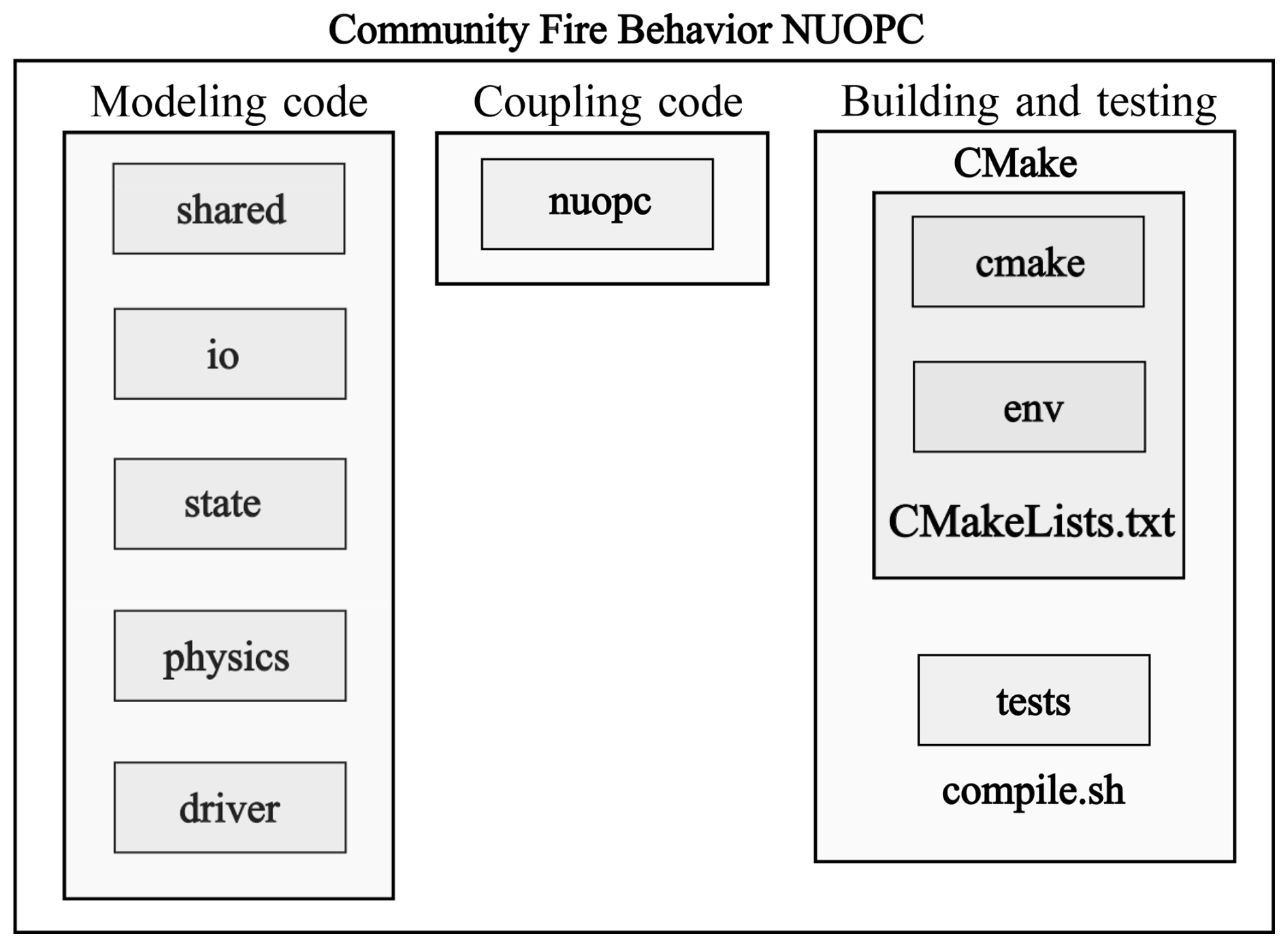
Figure 1 Diagram illustrating the organization of the CFBM code. Each box corresponds with a directory in the code.

2.1 The fire behavior model

The fire behavior model is based on WRF-Fire version 4.3.3. In WRF, the user defines an atmospheric domain and a refinement ratio that produces a finer horizontal grid spacing to compute fire processes. The result is a fire grid with a finer grid spacing, covering the same region as the atmosphere. To represent fire processes, it is also required to provide a fuel dataset, based on the 13-fuel categories from Anderson (1982) or the 40-fuel categories of Scott and Burgan (2005), and an elevation dataset to account for the high resolution topography on the fire grid. The elevation dataset is used to calculate the slope in the south-north and west-east directions, which is then used by the fire model to propagate the fire. Different elevation datasets can be used for the atmosphere and the fire given their different grid spacing. The domain configuration and the interpolation of the static datasets are performed by the Geogrid program which is part of the WRF Pre-Processing System (WPS). In the current version of CFBM, we also rely on the Geogrid program to define the fire grid and interpolate the static datasets, but, since there is no atmospheric component in CFBM, only the fuels and elevation (including slopes) in the fire grid are used. It is expected that future versions of CFBM will have its own preprocessing system.

Besides the Geogrid file, the only other file needed to run the model is the namelist (i.e., namelist.fire). Examples of the namelist are provided in the tests directories inside the tests folder (Fig. 1).

Ignitions can be performed in two ways. One option is to set up the ignition parameters in the fire namelist. The ignition can be a point, a circle, or a line ignition, and the ignition time is set up as seconds since the beginning of the simulation. The other option is to initialize the fire perimeter from observations (e.g. fire mappings from aircraft or satellites). The observations are used to initialize the level set function which defines the location of the fire front. The level set function is a signed distance function from the fire front, positive (negative) outside (inside) the fire perimeter (Mallet et al., 2009). Hence, at the fire perimeter the level set function is zero. The user is required to generate and add this initial level set function to the file generated by the WPS Geogrid program. This fire-perimeter initialization method is the only such approach available in WRF-Fire and has been successfully used in previous research with the WRF-Fire model (DeCastro et al., 2022; Turney et al., 2023). More sophisticated methods (e.g. Kochanski et al., 2023) could be explored in future versions of the model that will go beyond the existing WRF-Fire methods. The ignition time from the perimeter is also defined in the fire namelist as seconds from the beginning of the simulation.

Once a fire has been ignited, the fire front is propagated based on a parameterization of the fire rate of spread (R). Currently, only surface fires are considered and R is parameterized based on Rothermel (1972). R depends on the fuel characteristics, the surface winds, and the terrain slope using

$$\begin{array}{}\text{(1)}& R=R_{\mathrm{0}}(\mathrm{1}+{\mathit{\varphi }}_{\mathrm{w}}+{\mathit{\varphi }}_{\mathrm{s}})\end{array}$$

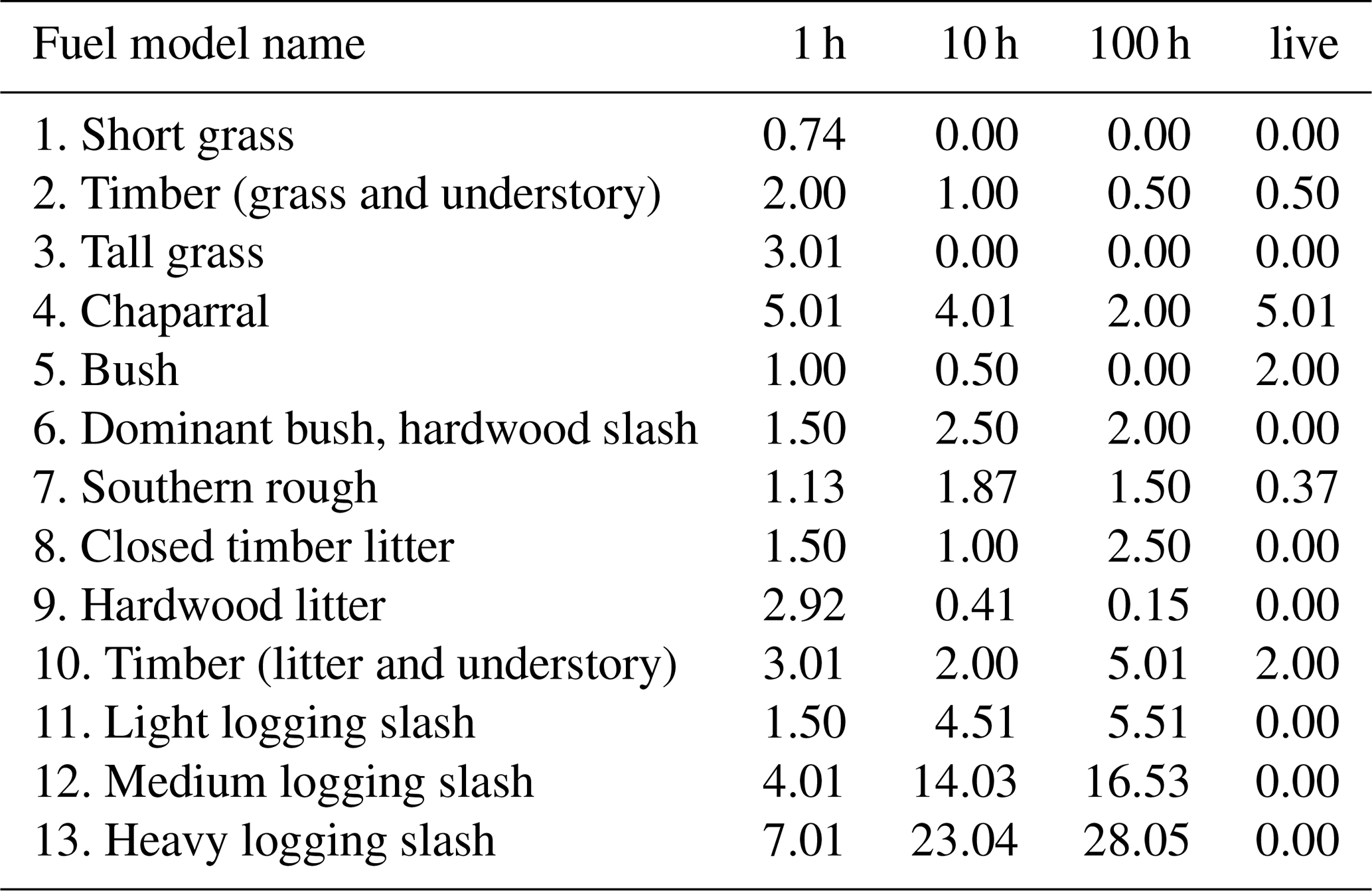
where R₀ is the rate of spread over flat terrain for a case with no wind; ϕ_w is the wind correction, and ϕ_s is the slope correction. The fire rate of spread is limited to a maximum of 6 m s⁻¹. A comprehensive description of each term involved in the parameterization is provided by Andrews (2018). R₀ depends on only the fuel characteristics. Some of the fuel characteristics are constant and others are a function of the fuel type defined by the 13 Anderson categories. The use of the more refined fuel models of Scott and Burgan (2005) is supported with a mapping of its 40 categories into the 13 categories of Anderson (1982). The fuel-dependent variables (Table 1) are the fuel load of the surface fuel, the fuel bed depth, the surface area to volume ratio, the characteristic time scale for burnout rates, and the fuel moisture content (FMC, the mass of water per unit mass of dry fuel) of extinction. The FMC can be either set to constant (8 % by default), or estimated dynamically using a FMC model (Mandel et al., 2014). If the FMC model is used, the mass of the surface fuels for 1, 10, 100, and 1000 h dead fuels and live fuels (Table 2) for each fuel type is also used. The constant characteristics are the ovendry fuel density (512.6 kg m⁻³), the fuel particle total mineral content (5.55 %), and the fuel particle effective mineral content (1.0 %). The fuel information is used to calculate R for the case of no wind and flat terrain (R₀). In the presence of winds, the wind correction, a function of the fuel characteristics and the surface wind, is also needed (ϕ_w). The surface wind responsible for the fire propagation are interpolations of the three-dimensional horizontal winds from the atmospheric component (see next section) to a height specified by the user in the namelist. This height represents the mid-flame height. Two interpolation options are available. The first one uses a linear interpolation on the logarithm of height from two adjacent model layers to the target height. In the second one, the user specifies a second height and the interpolation is performed from this height to the target height using the logarithmic wind profile. This second option was implemented to use upper-level winds less affected by the fire since Rothermel's parameterization was designed to use ambient winds. In the future, we intend to alleviate this subjective choice and implement the use of wind adjustment factors to automatically identify the height that drives the fire evolution based on the fuel characteristics (Eghdami et al., 2025). Similar to the wind correction term, the effects of the terrain slope are also accounted for by an additional term (ϕ_s). This term depends on fuel properties and the terrain slope. The only exception to the Rothermel rate of spread parameterization is the chaparral fuel model that uses a function that only depends on the wind speed (Clark et al., 2004). In this way, the fuel characteristics, winds, and terrain slope determine the fire rate of spread.

Table 1 Some characteristics of the Anderson's 13 surface fuel models used in the CFBM.

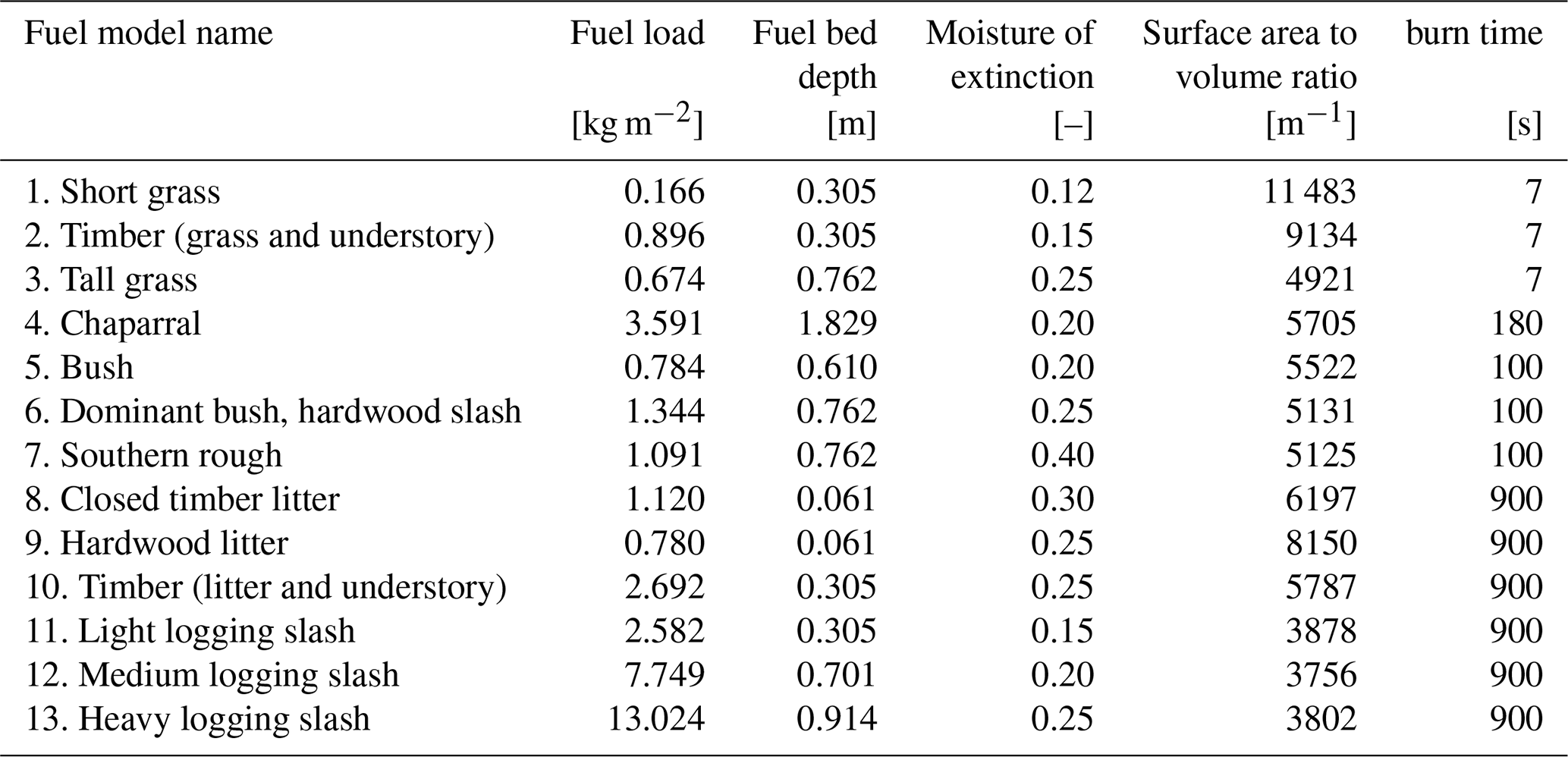
Table 2 Fuel loads for the 1, 10, 100 h and live fuels [kg m⁻²] for the Anderson's 13 surface fuel models. The 1000 h load is set to zero.

The rate of spread is used to propagate the fire by advancing the level set function (Mandel et al., 2011; Muñoz-Esparza et al., 2018). This is accomplished by numerically solving the level set equation:

$$\begin{array}{}\text{(2)}& {\displaystyle \frac{\partial \mathit{\phi }}{\partial t}}+R(\parallel \mathbf{\nabla }\mathit{\phi }\parallel -\mathit{ϵ}\mathrm{\Delta }\mathit{\phi })=\mathrm{0}\end{array}$$

where φ is the level set function, $\mathrm{\nabla }\mathit{\phi }=\left(\frac{\partial \mathit{\phi }}{\partial x},\frac{\partial \mathit{\phi }}{\partial y}\right)$, and ϵΔφ is an artificial viscosity stabilizer with $\mathrm{\Delta }\mathit{\phi }=\mathrm{\Delta }x\frac{{\partial }^{\mathrm{2}}\mathit{\phi }}{\partial x^{\mathrm{2}}}+\mathrm{\Delta }y\frac{{\partial }^{\mathrm{2}}\mathit{\phi }}{\partial y^{\mathrm{2}}}$, and ϵ the artificial viscosity constant. Here, R is the rate of spread of the fire normal to the fire front which is calculated using the wind speed and wind slope normal to the fire front in Rothermel's rate of spread parameterization (Eq. 1). The normal unit vector to the fire front needed for the projections is $\frac{\mathbf{\nabla }\mathit{\phi }}{\parallel \mathbf{\nabla }\mathit{\phi }\parallel }$. The level set equation is solved using a third order explicit Runge-Kutta scheme for the time integration. For the spatial derivatives, several methods are available. By default, the spatial derivatives are solved using the fifth-order weighted essentially nonoscillatory (WENO5) method around the fire front and a first-order essentially nonoscillatory (ENO1) method elsewhere. This allows for an accurate solution of the level set function near the fire front, while at the same time, minimizing the computational cost elsewhere when the value of the level set function is not relevant. The term representing the artificial viscosity requires two values of viscosity, one that is valid near the fire front and another that is valid elsewhere (by default the value of both viscosities is set to 0.4). The motivation for this is to allow for an accurate solution of the level set equation near the fire front, and facilitate stability of the numerical method. However, as the fire propagates, the level set function needs to be reinitialized to maintain its properties (signed distance function from the fire front). The reinitializations require solving the equation

$$\begin{array}{}\text{(3)}& {\displaystyle \frac{\partial \mathit{\phi }}{\partial \mathit{\tau }}}+S\left({\mathit{\phi }}_{\mathrm{0}}\right)(\parallel \mathbf{\nabla }\mathit{\phi }\parallel -\mathrm{1})=\mathrm{0}\end{array}$$

where $S\left({\mathit{\phi }}_{\mathrm{0}}\right)={\mathit{\phi }}_{\mathrm{0}}({\mathit{\phi }}_{\mathrm{0}}^{\mathrm{2}}+\mathrm{\Delta }{x}^{\mathrm{2}}{)}^{-\mathrm{1}/\mathrm{2}}$, φ₀ is the level set function after solving the level set equation (Eq. 2), and τ is a pseudo time (Sussman et al., 1994; Muñoz-Esparza et al., 2018). Considering the importance of reinitializing the properties of the level set function, reinitializations are activated by default. The reinitialization equation is also solved using a third order explicit Runge-Kutta scheme for the time integration and WENO5/ENO1 for the spatial derivatives. Solving the reinitialization equation requires iteration. One iteration is set as default based on our previous work (Muñoz-Esparza et al., 2018). Hence, the level set equation (Eq. 2) and its reinitialization equation (Eq. 3) are solved every time step in order to advance the level set function that tracks the evolution of the fire front.

After advancing the level set function, the fire can propagate into adjacent grid cells which are ignited as fire front passes. To refine the accuracy of the front propagation, each grid cell is further subdivided into four parts, and the level set function is interpolated to this refined grid, also allowing better estimate the burnt area and fuel consumption (Mandel et al., 2011). The fuel available to burn in a given grid cell depends on the fuel type (Table 1). The time it takes to burn the fuel is approximated with an exponentially decaying function (Clark et al., 2004; Mandel et al., 2011; Coen et al., 2013) which requires a characteristic time that also depends on fuel type (burn time in Table 1). The burn time produces a decrease of 40 % in the fuel amount in 10 min for a value of 1000 s, and it is translated to the e-folding time by dividing the burn time by 0.85 (Mandel et al., 2011). The combustion process generates heat and moisture fluxes that are parameterized. The heat release is represented with the following equation

$$\begin{array}{}\text{(4)}& \text{SH}=\mathrm{\Delta }m{f}_{\mathrm{dry}\mathrm{\_}\mathrm{fuel}}{h}_{\mathrm{c}}\end{array}$$

where SH is the kinematic sensible heat flux released by the ground fire [J m⁻² s⁻¹]; Δm is the fuel mass burned [kg m⁻² s⁻¹], f_{dry_fuel} is the fraction of dry fuel mass per fuel mass defined in terms of the FMC following $f_{\mathrm{dry}\mathrm{\_}\mathrm{fuel}}=\frac{\mathrm{1}}{\mathrm{1}+\text{FMC}}$; and h_c is the heat of combustion for dry cellulose (17.433 MJ kg⁻¹). The kinematic latent heat flux (LH [J m⁻² s⁻¹]) from the ground fire is

$$\begin{array}{}\text{(5)}& \text{LH}=\mathrm{\Delta }m(f_{\mathrm{water}}+f_{\mathrm{water}\mathrm{\_}\mathrm{in}\mathrm{\_}\mathrm{cellulose}}{f}_{\mathrm{dry}\mathrm{\_}\mathrm{fuel}})L_{\mathrm{v}}\end{array}$$

where f_water is the fraction of water in the fuel mass ($f_{\mathrm{water}}=\frac{\text{FMC}}{\mathrm{1}+\text{FMC}}$); f_{water_in_cellulose} is the fraction of water in cellulose released during combustion (56 %); and L_v is the latent heat of vaporization of water (2.5 MJ kg⁻¹). In addition to the heat and moisture fluxes, a fraction of the fuel burnt during the combustion, 2 % by default (following Coen, 2013), is released as smoke.

The procedures of the CFBM described above closely follow WRF-Fire methods, but important modifications have been introduced in the code. Using the same methods is desirable in the version 0.2.0 of the CFBM herein presented to ensure proper implementation as will be shown below. The WRF-Fire methods are mostly confined to the physics directory (Fig. 1). We have reorganized, modified and added substantial new source code (mostly in the directories not labelled as physics in Fig. 1) to create a standalone fire model, with built-in tests. We have also improved code clarity. Additionally, the code is more orthogonal in order to facilitate maintenance and future extensions. For the same reasons, we have added new derived types with their own type-bound procedures. For example, the most important physical processes that are parameterized have an abstract derived type with deferred procedures, and the derived type is extended with a particular parameterization of the process. Furthermore, procedures were reformatted to have a consistent format, and most of the code is self-documented to facilitate understanding of what is being done. Some procedures had arguments that were passed but not used, and these arguments have been removed. We also have incorporated the implicit none statement in all procedures, and, when possible, functions are declared as pure. A substantial number of consistency checks and prints through the code have been removed to improve readability and performance. The namelist options controlling the fire evolution have been simplified keeping only a reduced set. In addition, all the source code related to WRF's atmosphere has been removed from the fire modules in the physics directory. This includes removing procedures to interpolate atmospheric variables from the atmospheric grid into the fire grid. The interpolation procedures were used to interpolate the latitudes and longitudes from the atmosphere into the fire grid, and now the geolocation of the fire grid is calculated using the map projection information, as it is done in the atmospheric grid. The code is compliant with the Fortran 2008 standard.

CFBM can be run without any atmospheric component in idealized mode. This requires the user to define the winds and the fuels which are homogeneous across the fire domain. The size of the domain is also defined via the namelists. This allows one to test developments before coupling it with an atmospheric component.

The left portion of Fig. 1 shows the directories with the modeling code. The shared directory contains modules used to define the constants of the model, manage dates and times, and handle Lambert-Conformal projections used to initialize the latitudes/longitudes of the fire grid from the Geogrid file. It also contains abstract derived types with deferred procedures for fuels, the rate of spread parameterization, and the FMC model. These types are currently extended, or instantiated, with WRF-Fire approaches, but they can be extended with other methods in order to have different parameterization of these processes. The io directory contains modules to write to the standard output/error streams, to read the Geogrid file, the fire namelist, and WRF variables in the standalone mode. To facilitate the reading of Geogrid and WRF data (see next section), the io directory also includes a module with generic procedures to read data from NetCDF files. The state directory contains a module to defining state variables and methods to initialize variables, updating atmospheric variables in the standalone mode, and saving the state variables in a NetCDF file. There are two additional modules to divide the domain into tiles for the upcoming OpenMP parallelization, and to define a derived type to handle ignition line data and methods to ignite the prescribed fire lines. The fire code is located in the physics directory. This code includes modules with the fire driver, level set procedures, fire physics procedures, and the extension of the abstract types for (1) fuel type following Anderson (1982); (2) the fire rate of spread type following Rothermel (1972); (3) and the dynamic FMC model (Mandel et al., 2014). Finally, the driver directory has modules to initialize and advance the fire model that are used by a standalone program to perform offline fire behavior simulations and for online coupling with the atmosphere via the ESMF library as described in the following section.

2.2 Coupling with the atmosphere

2.2.1 Offline coupling

The CFBM can be driven by an existing WRF simulation in an offline manner in what we refer to as the standalone model. The standalone model was implemented to ensure consistency with WRF-Fire, and thus minimize the number of issues during the developments. With this aim, we generated automatic tests to check the output of a short run of the standalone model against the WRF-Fire solution. The standalone model does not need the fire grid, specified by the Geogrid output, to match the WRF domain. The only requirements are that the fire grid be within the extent of the WRF domain, and the WRF simulation has the required variables available. The interpolation of variables from the WRF atmospheric data into the fire grid uses a nearest-neighbour interpolation. We plan to include other interpolation methods in future versions of the model. These variables are the three-dimensional winds (U and V variables in WRF), the geopotential height (PH and PHB), the roughness length (ZNT), the 2 m temperature (T2), the 2 m water vapor mixing ratio (Q2), the precipitation (RAINC and RAINNC), and the surface pressure (PSFC). The surface pressure, precipitation, 2 m water mixing ratio, and 2 m temperature variables are only used if the FMC model is activated. In addition, the WRF projection must be Lambert-Conformal in CFBM version 0.2.0. Support for Mercator and polar stereographic projections will be added in future versions. The frequency to update the atmospheric state is controlled by a namelist setting. Although the standalone model was implemented to ensure consistency between WRF and the CFBM, the model is also useful for efficiently testing sensitivities in model parameters and methods defined in the fire namelist. This offline coupling can be extended to other atmospheric models having the basic atmospheric variables described above. The only external library required to compile the standalone fire code are the C and Fortran NetCDF libraries that are used for reading and writing procedures.

When connected to an atmospheric model using two-way coupling, the ESMF library is also required in order to pass the kinematic fire fluxes (Eqs. 4 and 5) and fire emissions to the atmosphere to account for fire–atmosphere interactions. The coupling framework is described in the following section.

2.2.2 Online coupling: The Community Fire Behavior NUOPC component

In order to couple the CFBM to an atmospheric model using the ESMF library, the CFBM is available as a NUOPC component. The NUOPC layer has been proven to promote interoperability as seen in the Earth System Prediction Suite (Theurich et al., 2016). This means that one modeling component codebase implemented as a NUOPC can be used in multiple Earth system modeling applications.

NUOPC compliance requires a standardized wrapper around the model code. This lightweight interface is commonly referred to as the “NUOPC cap”. The cap is responsible for initializing the model, including the definition of the fire grid from the Geogrid file, and to coordinate its advancement with other Earth system components. To this end, we use the fire initialization subroutine and the subroutine that advances the fire state one time step. The NUOPC cap also bundles all of the necessary coupling requirements into import and export states. The variables that are mandatory to import are the 3 dimensional winds and geopotential height, the roughness length, the 2 m temperature, the 2 m water vapor mixing ratio, the surface pressure, and precipitation. Precipitation can be passed either as a precipitation rate or as accumulated precipitation since the beginning of the simulation. The variables that can be exported are the kinematic sensible heat flux and the kinematic latent heat flux released from the fire (Eqs. 4 and 5), and the fire smoke emissions. This strategy to import/export variables differs from inline coupling where data structures pass directly between components, which would require explicit knowledge of the atmosphere component's code. Built into the NUOPC interoperability layer is the ESMF and therefore regridding between the different grids across the Earth system components. In the fire NUOPC cap, we also perform the vertical interpolation of the 3-dimensional horizontal winds into a 2-dimensional array with the winds at the target height above ground level to propagate the fire.

The middle portion of Fig. 1 shows the directory providing the ESMF functionality. This is the nuopc directory which contains the fire NUOPC cap. It connects to the fire model via the initialization and advance subroutines available in the driver directory. The NUOPC directory also has files to create an Earth system model (fire driven by an atmospheric component) that we use for testing purposes as will be described in the following section.

2.3 Compilation and testing

The organization of the code related to compilation and testing is shown in the right portion of Fig. 1. The automatic compilation of the code is implemented with CMake. A bash script, compile.sh, is used to compile the code and test it if instructed. The test is designed to minimize the number of potential issues introduced into the code. The test runs a series of short simulations of the fire evolution and compares results against the known solution. The test can check the offline or standalone model (Sect. 2.2.1) build, and the NUOPC build (Sect. 2.2.2). Checking the offline model is straightforward, as it simply requires having a previously run WRF simulation. In order to test the online coupling via the NUOPC, we have created a WRF-data NUOPC component. The WRF-data NUOPC component only has the cap since the WRF-data NUOPC component just reads variables from the output of an existing WRF simulation. The cap defines the WRF-data grid, from the Geogrid file, and imports the variables that the fire NUOPC component needs. This is a one-way coupling from the atmosphere to the fire and therefore behaves as the standalone model described in the previous section. The main difference is that this coupling requires ESMF whereas the standalone code described before does not. The regridding from the atmospheric grid to the fire grid is performed by the ESMF library. The diagram shown in Fig. 2 summarizes the coupling strategy between the Earth system model coupling the WRF-data NUOPC component and the CFBM NUOPC component which is used for testing purposes. NUOPC caps have been written for each model, which allows data to pass from one component to another through NUOPC connectors (arrow). NUOPC connectors are built into NUOPC and redistribute or regrid data between connected pairs of components.

The Earth system model connecting the fire and the WRF-Data NUOPC caps that is built for testing uses ESMF or the Earth System modeling eXecutable (ESMX). The ESMF build is the standard, and requires additional code with the NUOPC driver that connects the components, and this code is available in the nuopc directory (Fig. 1). The ESMX application is a community oriented application that builds a NUOPC coupled system, the Earth system model, containing NUOPC compliant components, the CFBM and WRF-Data components in this case, without creating or maintaining the NUOPC driver. Components are added to or removed from an ESMX build through configuration files written in YAML therefore eliminating the need to write code. Hence, using the ESMX extension reduces the amount of code to build the Earth system application, and thus allows for faster developments and easier maintenance. The ESMX build includes an extra test that utilizes an ESMX Data component to prescribe meteorological forcing values. The forcing values are exported to the CFBM which then returns kinematic sensible heat flux and the kinematic latent heat fluxes to the ESMX Data component for validation. These tests, as well as all the offline tests, run nightly to ensure the CFBM and CFBM cap do not break during development. Furthermore, any system utilizing ESMX as its application can embed the CFBM component. Our fire NUOPC component has been an early adopter of the ESMX technology and both coupling strategies, ESMF and ESMX, are being tested.

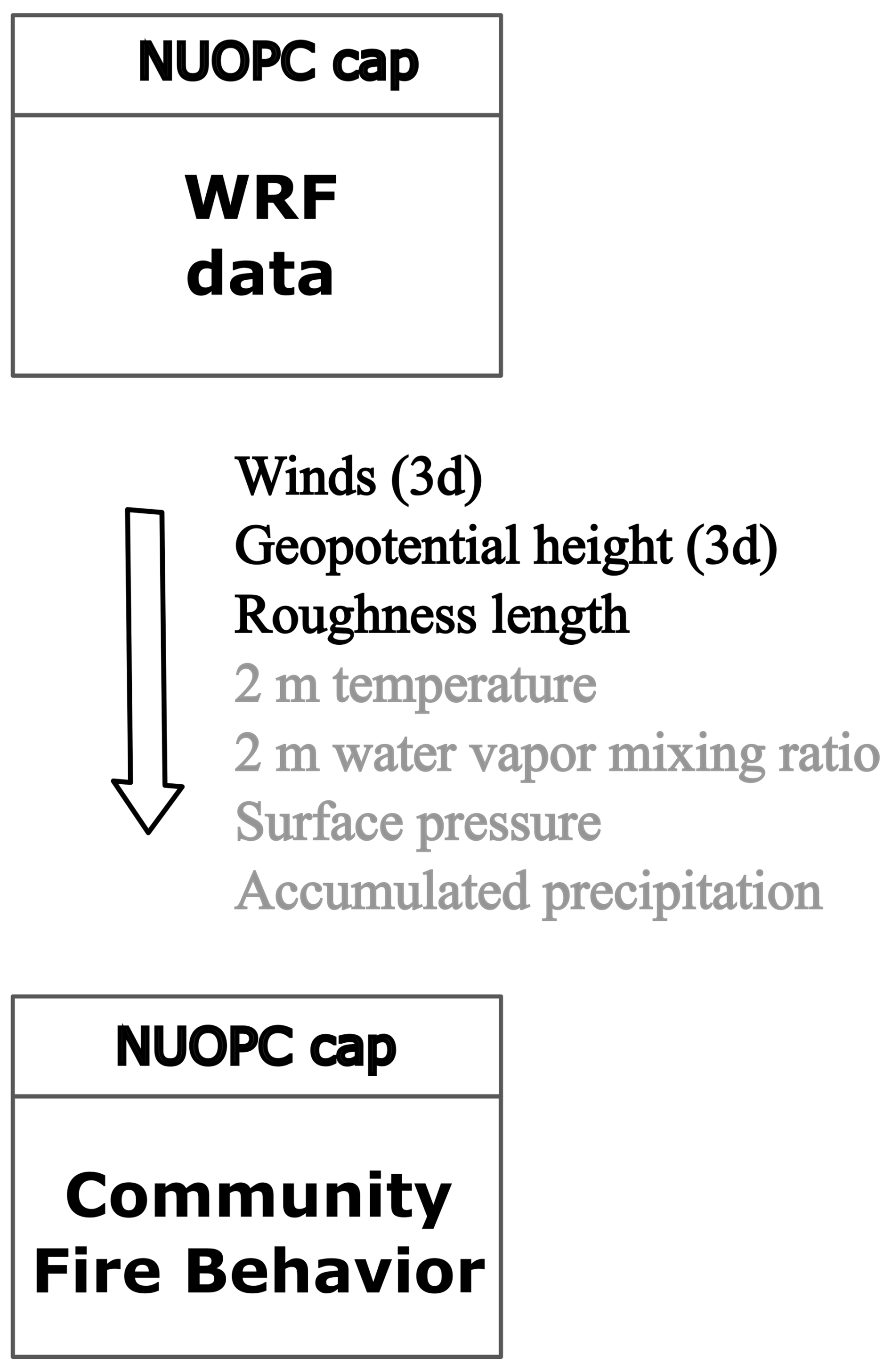
Figure 2 Diagram illustrating the WRF-data NUOPC component and the CFBM NUOPC component with the variables that exported (imported) by WRF-data (Fire behavior). The variables in gray are only used if the fuel moisture content model is activated to simulate the moisture content dynamically.

The tests are included in the tests directory (Fig. 1). Currently, there are two tests implemented with and without activating the FMC model. The github repository of the CFBM also runs the tests every time there is a new code development pushed to the repository to minimize the introduction of bugs in the code.

The only necessary libraries to compile and test the code are NetCDF and ESMF (the latter one only for the NUOPC builds). The code can also be built with MPI libraries. Parallelization is not supported in version 0.2.0, but MPI compilation is included in order to couple CFBM with UFS that uses MPI-based compilation. In this way, the CFBM model can be integrated into an MPI parallelized application but at this time the CFBM model runs serially on a single processor. The CFBM model includes MPI library linking for future development. CMake is able to find these three libraries in the user environment. To ensure reproducibility and ease of use, the environment used to build executables and run tests can be automatically configured, via adding –env-auto to the compile script. This flag then locates a bash script that loads modules and defines environment variables for defined systems. At the time of writing, the only computer in env is Derecho, a high performance computer that is part of the NSF NCAR-Wyoming Supercomputer Center. New systems can be defined by adding a <system_name> directory containing bash configuration files. The new system must then be added to the “auto environment” section of the compile script.

3 Coupling the Community Fire Behavior model to the UFS

The UFS has its components implemented as NUOPC components (e.g., atmosphere, ocean, land, etc.) to facilitate their coupling. Hence, we have coupled the CFBM NUOPC component to the UFS-Atmosphere NUOPC component using the existing infrastructure.

The coupling diagram illustrating the combined UFS-Atmosphere and the CFBM is shown in Fig. 3. The UFS has other NUOPC components that are not illustrated here since it is possible to just run the UFS-Atmosphere together with the fire component. The variables imported by the fire NUOPC component are similar to the ones imported for the case of the WRF-data NUOPC component (Fig. 2), but the accumulated precipitation has been replaced by the precipitation rate. Comparison of Figs. 2 and 3 serves to illustrate that a single NUOPC cap written for CFBM is agnostic to the external atmosphere being coupled. Differences being that a completely different atmospheric component, whether data or not, can be coupled therefore creating an entirely different coupled Earth system model. In this case, a main difference is the feedback provided by the fire NUOPC component to the atmosphere via sensible and latent heat fluxes released by the fire. This allows for two-way coupling between the two components if desired. In practice, the user decides if the coupling is one way (information from the atmosphere to the fire only) or two ways (one way plus adding the fire feedback to the atmosphere component) via the fire namelist. Smoke emissions as a result of burning the surface fuels by the fire model are also passed to the atmosphere.

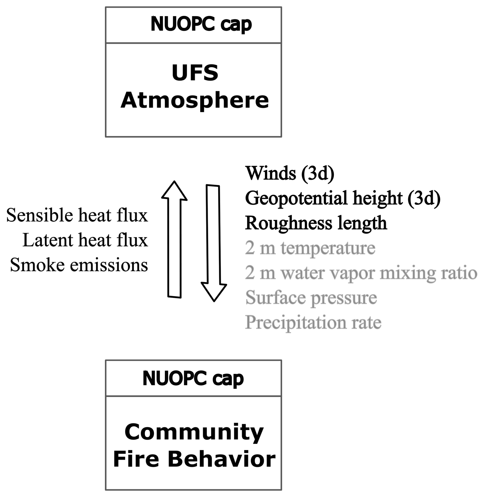
Figure 3 Diagram illustrating the UFS-Atmosphere NUOPC component and the CFBM NUOPC component with the variables that are exported (imported) by the fire behavior (UFS) on the right, and the variables that are exported (imported) by UFS (Fire behavior) on the right. The variables in gray are only used if the fuel moisture content model is activated to simulate the moisture content dynamically.

In UFS, the physical processes, or parameterizations, are represented using the Common Community Physics Package (CCPP, Heinzeller et al., 2023). It is inside CCPP wherein the kinematic fluxes from the fire (Eqs. 4 and 5) are used to update the temperature and moisture tendencies. This is done in the fluxes wrapper. Originally, the wrapper combined surface fluxes from the land, ocean, and ice, but we extended the functionality to include the fire fluxes. The kinematic flux divergences are added to the temperature and moisture tendencies of the first atmospheric layer. The smoke emissions are added to the first atmospheric layer of a passive tracer to represent the smoke transport and dispersion associated with atmospheric dynamics. A more comprehensive coupling of the smoke with radiation and cloud microphysics is left for future work.

To facilitate running coupled fire–atmosphere simulations with UFS, we have incorporated the fire behavior model into the UFS Short-Range Weather App (SRW App). This is the application that is used to run UFS-Atmosphere in a regional, limited-area configuration, with a workflow that conveniently links pre-processing, running, and post-processing of the model, with a single configuration file ensuring all components are linked and run together in a self-consistent way. This contribution is a mutually beneficial relationship: the CFBM gets a robust, well-supported workflow for running experiments coupled to an atmospheric model on a wide range of computational platforms, and the UFS community receives new capabilities for fire prediction experiments within the existing, familiar and well-documented framework of the SRW App. With this new capability contributed to the publicly available and supported SRW App, one can perform fire–atmosphere simulations without altering the steps required to run a conventional atmospheric simulation, using a workflow that allows for easy modification of domains, dates, and other configurable options of the atmospheric component in a way that is consistent with the fire component.

Currently, the main limitation is that CFBM can run with just one dynamical core, but we are working to include OpenMP parallelization soon. However, the region covered by the fire simulation in CFBM does not need to match the atmospheric domain allowing for using smaller fire domains which reduces the computational requirements of the fire model. Also, it is possible to have any kind of atmospheric grid (e.g., unstructured) and the NUOPC cap will perform the interpolation of variables automatically.

4 Model inter-comparison: testing the Community Fire Behavior NUOPC component and its coupling with UFS

The version 0.2.0 of the CFBM herein presented closely follows WRF-Fire methods (see description in Sect. 2.1) in order to compare results between the CFBM NUOPC component implemented in UFS and WRF-Fire results. This allows us to ensure a proper implementation in order to have a starting point to introduce further developments to improve the realism of the fire simulations in subsequent studies. In order to test the implementation, we have performed idealized simulations as well as simulations for a real fire event.

The idealized simulations replicate our previous study with WRF-Fire to test the performance of the level set method in tracking the location of the fire front (Muñoz-Esparza et al., 2018). The simplicity of the idealized simulations, with homogeneous winds and fuel characteristics, provides one with a theoretical solution of the location of the fire front which is the benchmark for comparison with different numerical methods used to resolve the level set partial differential equation (Eq. 2).

For the real fire, we have selected a wildland fire over complex terrain in Colorado, U.S., the Cameron Peak Fire, and configured UFS and the CFBM similar to the WRF-Fire configuration to compare the consistency of results. In spite of having a very similar configuration of the models, identical results are not expected considering the different dynamical cores, differences in the implementation of parameterizations, and the nonlinear behavior of the atmosphere; but the fire evolution should be similar considering the close experimental set up between the models.

4.1 Experimental set up

4.1.1 Idealized case

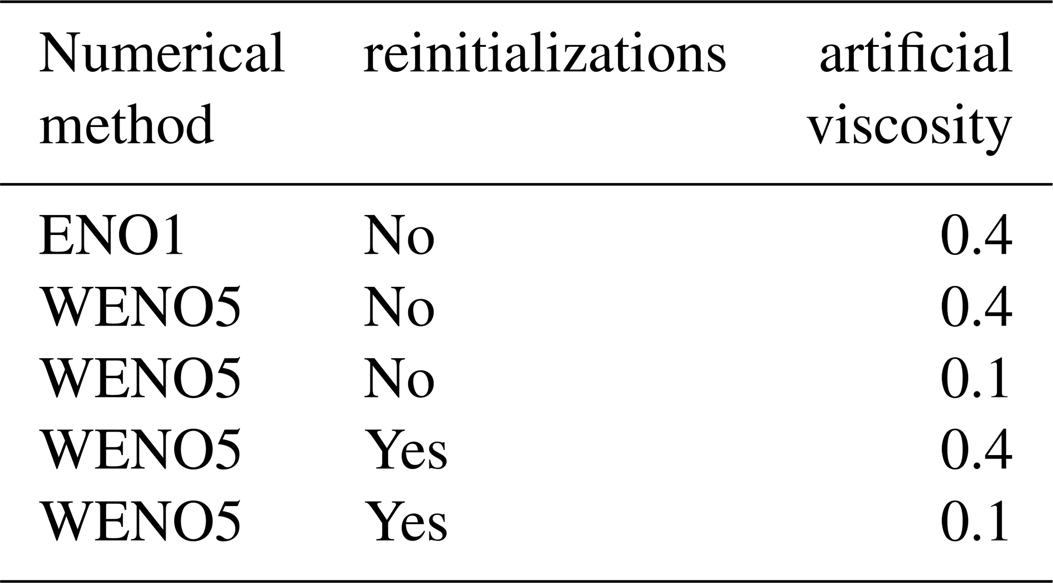
The idealized case simulates the fire evolution of a meridional ignition line driven by westerly winds. The westerly winds are constant, 4.55 m s⁻¹, over the whole domain (2 km by 5 km grid). The fuels are also homogeneous and set to short grass. The grid spacing is set to 25 m. Five simulations are performed using different methods to resolve the level set equation (Eq. 2). The experiments differ in the numerical method (ENO1 or WENO5), the activation of the reinitialization of the level set function (no reinitialization or 10 iterations), and the value of the artificial viscosity (0.4 or 0.1), and are summarized in Table 3. The performance of the experiments is assessed by comparing results after 35 min of simulation with the theoretical location of the fire front which is calculated based on the rate of spread of the fire (Eq. 1).

Table 3 Description of the idealized simulations performed.

4.1.2 The Cameron Peak fire

In order to test the adequacy of the CFBM developments and its coupling to UFS, we inspected the consistency of results from simulations using UFS-CFBM, WRF-Fire, and the standalone CFBM for the Cameron Peak fire. The Cameron Peak Fire started on 13 August 2020 at approximately 20:00 UTC (02:00 p.m. MDT) on the Arapaho and Roosevelt National Forests, west of Chambers Lake in northern Colorado. The fire started East of Cameron Peak, on a hot, dry, and windy day with gusts reaching 32 m s⁻¹. The fire spread quickly through the mountainous terrain and beetle-killed trees in the region. The fire was contained on 5 December 2020 with an estimated area of around 209 000 acres, representing the largest wildfire perimeter in Colorado's history.

In this work, we focus on approximately the first 28 h of the fire evolution to minimize the effects of human intervention. Three fire perimeters are available during this period from the Colorado Wildfire Information Management System (CO-WIMS) database. The first perimeter, hereafter referred to as Perimeter-1, corresponds to 13 August 2020, 23:42 UTC (05:42 p.m. MDT), the second perimeter, Perimeter-2, to 14 August 2020, 15:54 UTC (09:54 a.m. MDT), and the last perimeter, Perimeter-3, to 14 August, 22:16 UTC (04:16 p.m. MDT).

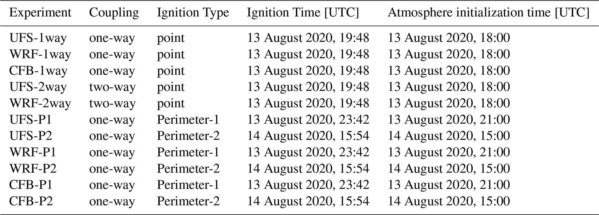
A total of 11 fire simulations were performed using either WRF version 4.3.3, UFS, or the standalone CFBM version 0.2.0 (Table 4). A few minor changes were introduced to WRF version 4.3.3. First, we update the atmospheric roughness length used by the fire model every time step since it varies between the first time step and subsequent ones. Second, we decreased the pseudo time for reinitializations by a factor of 100 to avoid numerical instabilities. And third, we fixed the VEGPARM.TBL to correct for missing/incorrect lines, this fix being a bugfix part of the official WRF release. The FMC model was not activated in the experiments since this is the default option in WRF-Fire. Instead, FMC was set to its default constant value, 8 %. Besides the atmospheric models, the experiments differ in the type of ignition (point ignition or from a perimeter) and the fire–atmosphere coupling strategy (one-way or two-way).

In the point ignition experiments, we simulate the initial 28 h of the fire evolution, corresponding to a 30 h model simulation period from 13 August 2020, 18:00 UTC, to 15 August 2020, 00:00 UTC. The ignition point was set to 40.609° latitude and −105.879° longitude, with 250 m radius, and it ignited from 6480 to 7000 s after initialization. The first three experiments in this set, UFS-1way, WRF-1way, and CFB-1way are configured with one-way feedback, meaning the atmosphere affects the fire but the atmosphere does not respond to the fire (i.e., uncoupled). This is the simplest configuration of the models and thus a good first step to assess the consistency between simulations. In the following experiments, UFS-2way and WRF-2way, the feedback from the fire to the atmosphere is activated. No simulation is performed with the standalone CFBM since the standalone code can only run in one-way mode.

In the remaining experiments, the fire is ignited from an observed perimeter. The UFS-P1, WRF-P1, and CFB-P1 are initialized from Perimeter-1, whereas UFS-P2, WRF-P2, and CFB-P2 are initialized from Perimeter-2. These six experiments do not pass information from the fire to the atmosphere (one-way coupling) since the standalone code only runs in one-way mode and the objective is to compare the consistency of the simulations. The perimeters were ignited at their corresponding timestamps, and the atmospheric state was initialized according to the closest model cycle used for initial condition (3-hourly intervals), i.e., 13 August 2020, 21:00 UTC for Perimeter-1 and 14 August 2020, 15:00 UTC for Perimeter-2. This leaves 2.7 h of spin up for the Perimeter-1 runs and 0.9 h for the Perimeter-2 runs.

Table 4 Description of the simulations performed for the Cameron Peak fire. The experiments labelled with CFB use the CFBM with the atmospheric information from the equivalent one-way WRF experiment.

The atmospheric models WRF and UFS ran with initial and boundary conditions from the High-Resolution Rapid Refresh (HRRR, Benjamin et al., 2016; Dowell et al., 2022) model at 3-hourly intervals. The simulations were configured with a single domain covering the state of Colorado at 1 km horizontal grid spacing. The WRF domain has 629 by 599 grid points whereas the UFS domain has 599 by 570 grid points. Although going to finer grid spacing is desirable to better represent fire–atmosphere interactions using a turbulence resolving mode based on large-eddy simulation (LES), this is not possible with UFS because it currently lacks an LES approach. Hence, we use 1 km because is at the limit of what can be achieved with traditional planetary boundary layer parameterizations available in both UFS and WRF. Grid spacings finer than 1 km are within the “gray zone” or “Terra Incognita” (Wyngaard, 2004) where turbulence starts to be explicitly resolved, and thus not easy to parameterize. For WRF, we used a fire grid refinement of 10 to reach a 100 m grid spacing in the fire grid. A smaller domain centered over the fire with 100 m grid spacing and 200 by 200 grid points was used when the CFBM was used (UFS and CFB experiments in Table 4). Hence, both UFS and WRF use a fire domain of 100 m grid spacing which is sufficient to capture the main heterogeneities in fuels and elevation over the region. The fuel and elevation data are generated by Geogrid in both models which is desirable for our main purpose of checking consistency between both models. Both models used the same number of vertical layers, 65, and the same time step of 4 s. The atmospheric data necessary to run the CFB experiments came from the equivalent one-way WRF experiment. In all the simulations, we used the Anderson 13-fuels obtained from the LANDFIRE database. Finally, we set the fire wind height to 2.5 m in all the simulations. This experimental setup provides a very close configuration of both WRF and UFS.

We also used the same parameterizations in all our experiments. In WRF, the physics processes were modeled with the following parameterizations: Thompson microphysics (Thompson et al., 2008); the Rapid Radiative Transfer Model for Global models (RRTMG, Iacono et al., 2008) for long and shortwave radiation; Mellor-Yamada Nakanishi and Niino (MYNN) Level 2.5 for the planetary boundary layer parameterization (Olson et al., 2019) and the surface layer parameterization (Olson et al., 2021), and the Rapid Update Cycle (RUC) land Surface Model (Benjamin et al., 2004). For UFS, the physics parameterizations were set to the CCPP FV3-HRRR which use the same parameterizations as in WRF. The experiments using the standalone CFBM (CFB-1way, CFB-P1, and CFB-P2) use atmospheric data from the WRF model. The atmospheric fields were provided in 20-min intervals. Effectively, this means the atmosphere runs with an identical configuration used by the WRF simulation, whereas the fire behavior component receives updates at 20 min intervals.

It will be shown that at 1 km grid spacing the fire feedback to the atmosphere produces a small impact. However, the impacts are sufficient to assess the consistency between WRF and UFS fire simulations which is the main objective of this model inter-comparison experiment. To quantify the agreement between the simulated fire perimeters we use the Heidke skill score (Wilks, 2011). A perfect agreement receive a Heidke skill score of one, and a prediction equivalent to the reference forecasts, the proportion correct that would be achieved by random forecasts that are statistically independent of the observations (Wilks, 2011), receive zero scores. Forecasts worse than the reference receive a negative Heidke skill score.

4.2 Results

4.2.1 Idealized simulations

Figure 4 summarizes the results of the idealized experiments. It shows the simulated fire perimeters after 35 min of the line ignitions for the five experiments performed (Table 3). The dashed vertical line on the right of the figure shows the expected location of the fire front after 35 min. The experiment using ENO1 (red line) is the one showing the largest discrepancy as a result of the larger numerical dissipation introduced by this numerical scheme with respect to WENO5. For the WENO5 experiments, reducing the artificial viscosity from 0.4 to 0.1 contributes to improving the agreement with the theoretical results (yellow and purple lines). Similar results to the WENO5 experiment with 0.1 artificial viscosity can be obtained by keeping the artificial viscosity to 0.4 but activating the reinitializations of the level set function (Eq. 3, light blue line). The fire front from this experiment is very close to the theoretical solution. Even better results can be obtained by reducing the artificial viscosity to 0.1 (dark blue line). These results are in agreement with a similar experiment based on WRF-Fire (Muñoz-Esparza et al., 2018) and it is the first indication of the adequacy of the CFBM developments.

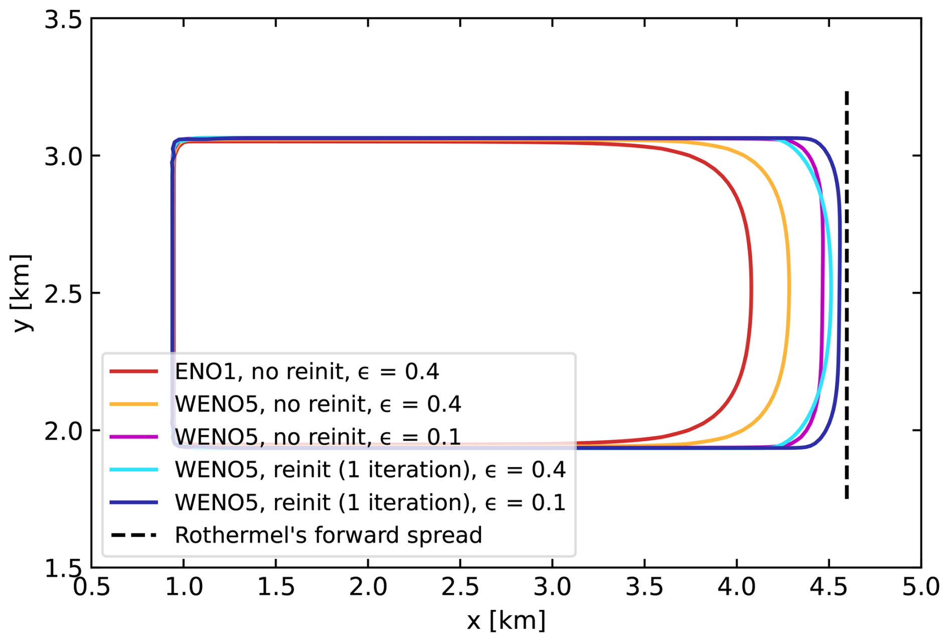
Figure 4 Location of the fire perimeter after 35 min of fire evolution for the idealized simulations using different numerical methods to resolve the level-set equation (see legend). The fire starts as a line ignition in the left side of the domain.

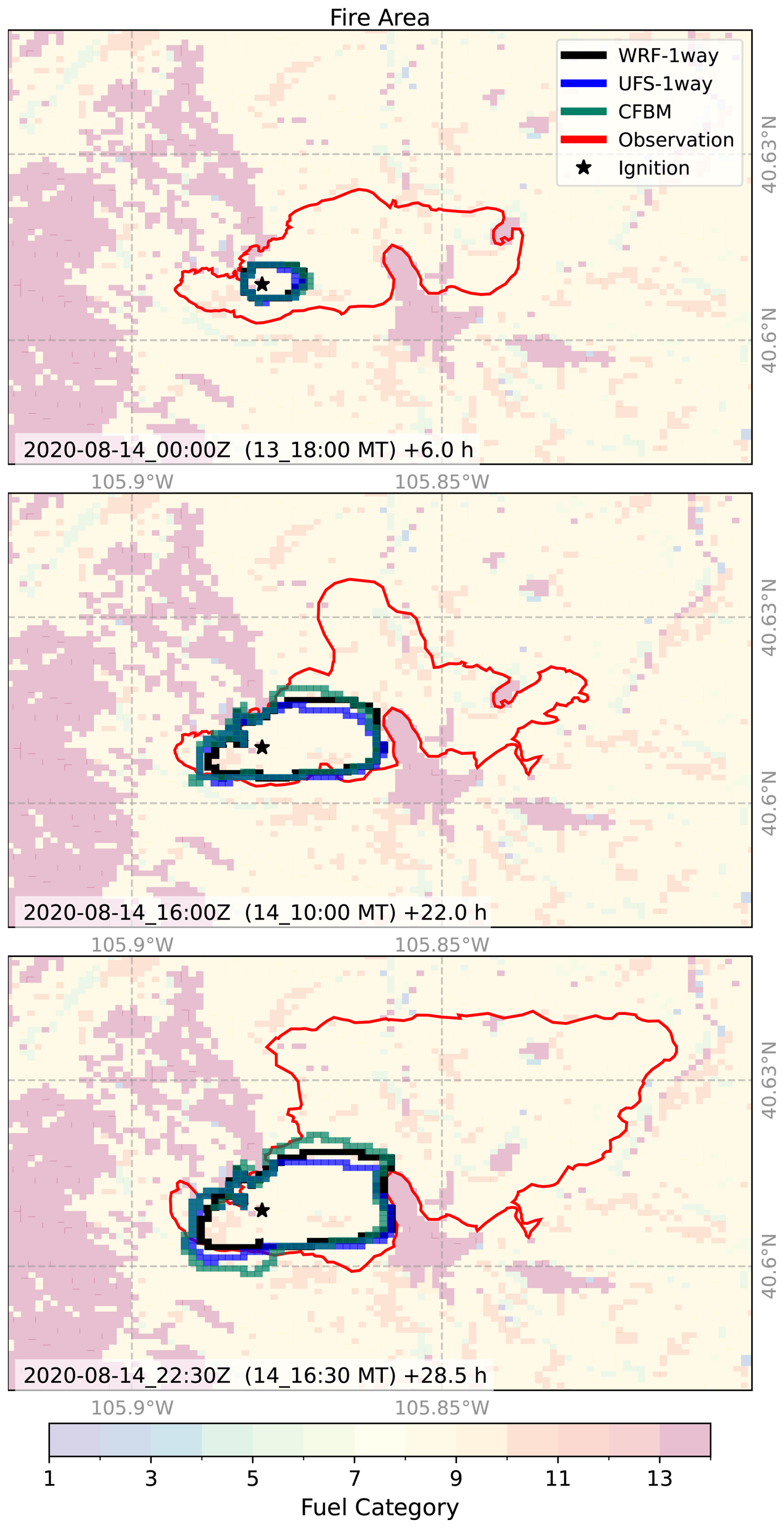
Figure 5 Simulated fire perimeters from experiments WRF-1way (black line), UFS-1way (blue line), and CFB-1way (green line) at the three times with available observations. The observed perimeters are also shown (red lines).

4.2.2 Point ignition: one-way simulations of the Cameron Peak Fire

Figure 5 shows a comparison of the simulated fire area for the one-way simulations that start the fire from a point ignition (UFS-1way, WRF-1way, and CFB-1way) and the observed perimeters from CO-WIMS. As expected, the three simulations, WRF-1way (black), UFS-1way (blue), and CFB-1way (offline coupling of WRF and the fire behavior model, green) show consistency in the simulated fire perimeters. A perfect match is not expected considering WRF and UFS are different atmospheric models and the standalone code only uses a fraction of the WRF atmospheric data and even a different interpolation from the atmospheric grid to the fire grid. In spite of these differences, the perimeters show good consistency with a Heidke skill score around 0.9 (Fig. 6), suggesting a proper implementation of the fire behavior model in the CFBM and its coupling with UFS. Although the comparison between simulation and observation shows the simulated fire underestimate the observed fire rate of spread, the simulations show consistent results among themselves. The underestimation with respect to observations is at least partially a result of inaccuracies in the ignition time and location records, and on the perimeter timestamps used to verify the simulations.

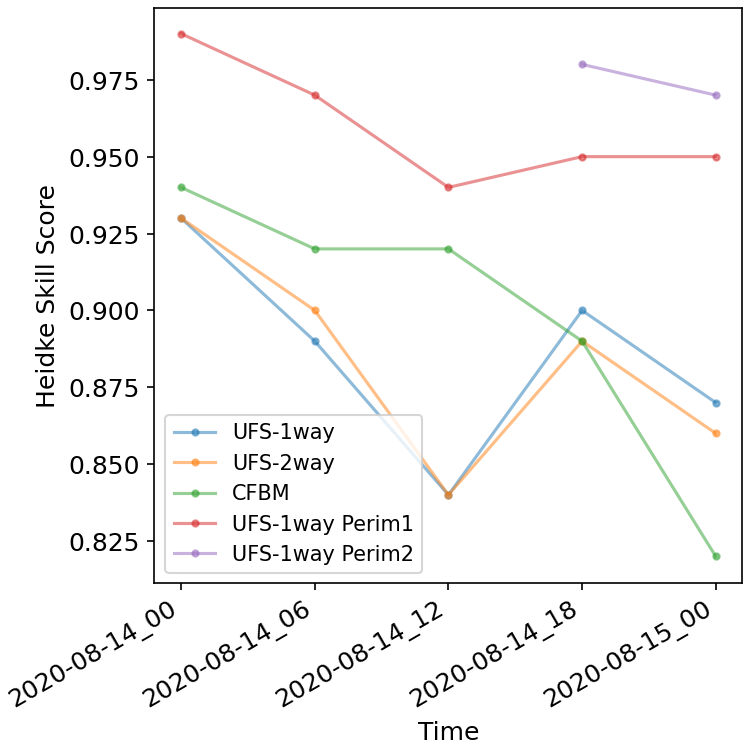
Figure 6 Heidke skill score comparing the simulated perimeters from UFS to the WRF-Fire results. The simulation labelled as CFBM is the standalone run driven by WRF data and has been compared against WRF-Fire results.

The consistency among the simulations is further illustrated in Fig. 7 which shows the evolution of the mean wind at the fire perimeter and the burned area. The mean wind speed at the fire perimeter (Fig. 7, right panel) is mostly between 1 and 3 m s⁻¹ and there is consistency in the three simulations (UFS-1way, WRF-1way, and CFB-1way). The mean bias error (MBE) and mean absolute error (MAE) between UFS-1way and WRF-1way are −0.3 and 0.5 m s⁻¹, respectively. For the comparison between WRF-1way and CFB-1way the MBE and MAE are 0.1 and 0.2 m s⁻¹, respectively. The variability is also similar with a correlation coefficient of 0.69 between UFS-1way and WRF-1way, and 0.87 between WRF-1way and CFB-1way. Again, discrepancies between the CFB-1way and WRF-1way experiments are expected because we use different interpolation methods to interpolate the wind speed to the target location, and the WRF data is updated only every 20 min in the CFB-1way experiment. Discrepancies between UFS-1way and WRF-1way experiments are also affected by different interpolation methods, but, more importantly, by different dynamical cores. However, in spite of these differences, we expected similar wind evolution in both simulations because we used the same HRRR forcing for initial and lateral boundary conditions. This agreement is evident in Fig. 7 (right). The wind consistency translates into a similar evolution of the burnt area (Fig. 7, left). CFB-1way shows larger differences because there are larger winds than WRF at the beginning of the simulation that conditions the evolution of the fire. The similarities between WRF-1way and UFS-1way are remarkable considering these are different atmospheric models.

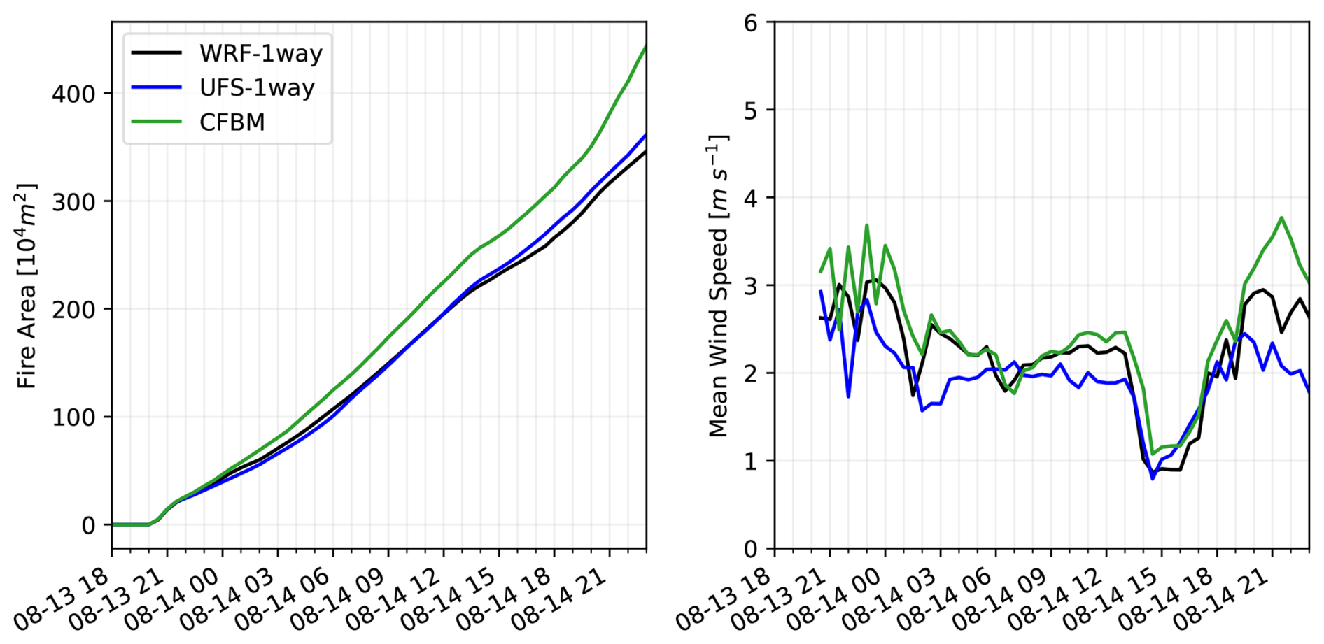
Figure 7 Evolution of the burnt area (left) and mean wind speed at the fire front (right) for experiments WRF-1way (black line), UFS-1way (blue line), and CFB-1way (green line). The wind speed corresponds to the wind at 2.5 m above ground level. The fire front is defined as the grid cells that are burning.

4.2.3 Point ignition: two-way simulations of the Cameron Peak Fire

After ensuring consistency of the perimeter evolution in one-way coupled simulations, we turn our attention to the two-way coupled experiments (WRF-2way and UFS-2way) that also allow for inspecting fire fluxes and atmospheric interactions. The comparison of the simulated and observed fire areas is shown in Fig. 8. Again, although we see an underestimation of the observed burned area, there is consistency between the simulated perimeters using WRF and UFS with a Heidke skill score around 0.9 (Fig. 6). Indeed, results are similar to the ones obtained with the one-way experiments (Fig. 5). The relatively small impact of the fire heat and moisture fluxes in these experiments is due to the use of 1 km grid spacing in the atmosphere, which results in the dissipation of the fire fluxes over a significantly larger area than the one where they were produced. We further show the evolution of the burnt area and the wind speeds calculated with the one-way and two-way experiments using WRF and UFS (Fig. 9). The two-way experiments show small differences with respect to their one-way counterparts. Again, there is consistency between the two-way results of UFS and WRF for both the evolution of the wind speed at the fire front and the burnt area.

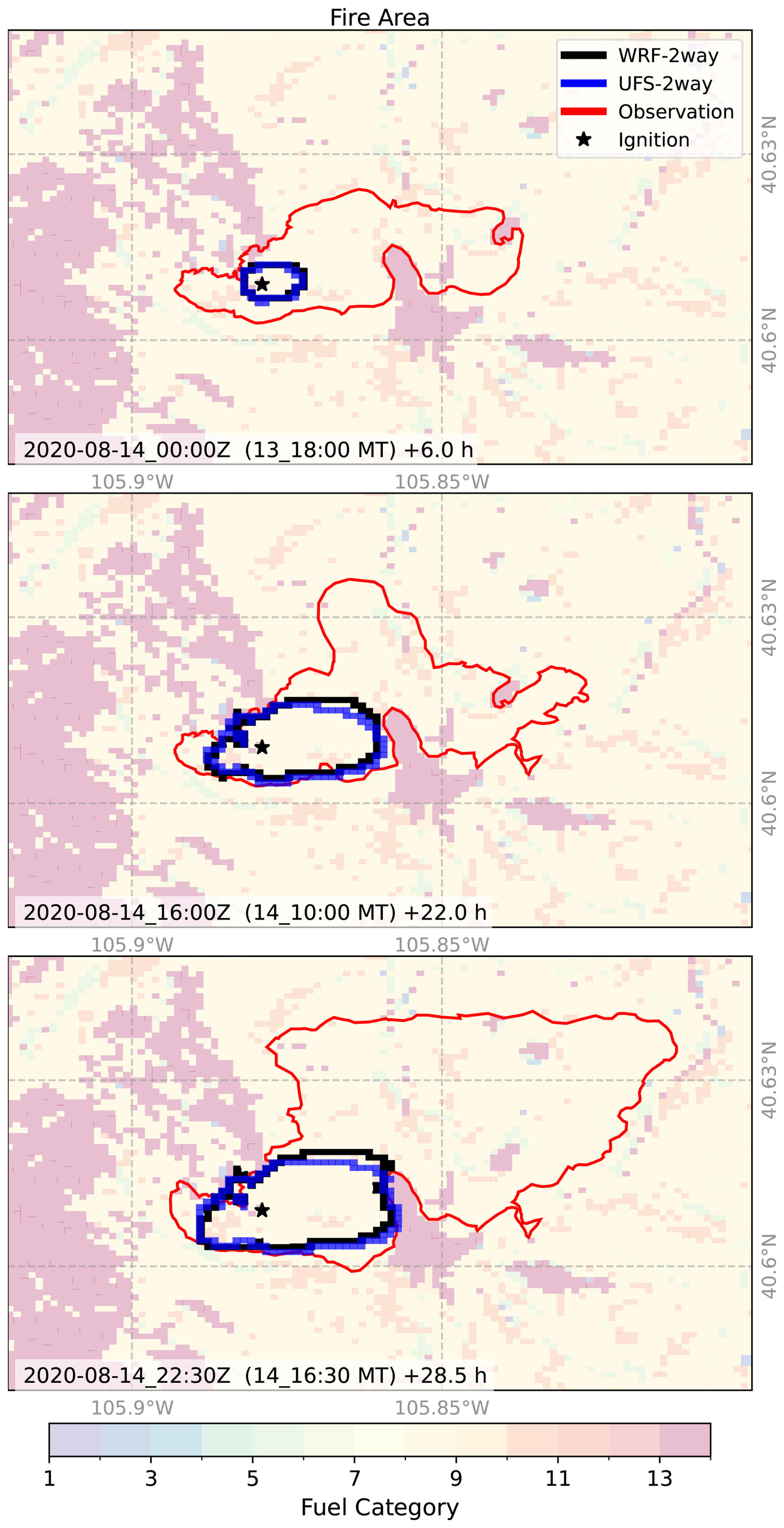
Figure 8 Same as Fig. 5 but for the WRF-2way and UFS-2way experiments. Results for the CFBM are not shown because the model can not be run with two-way coupling.

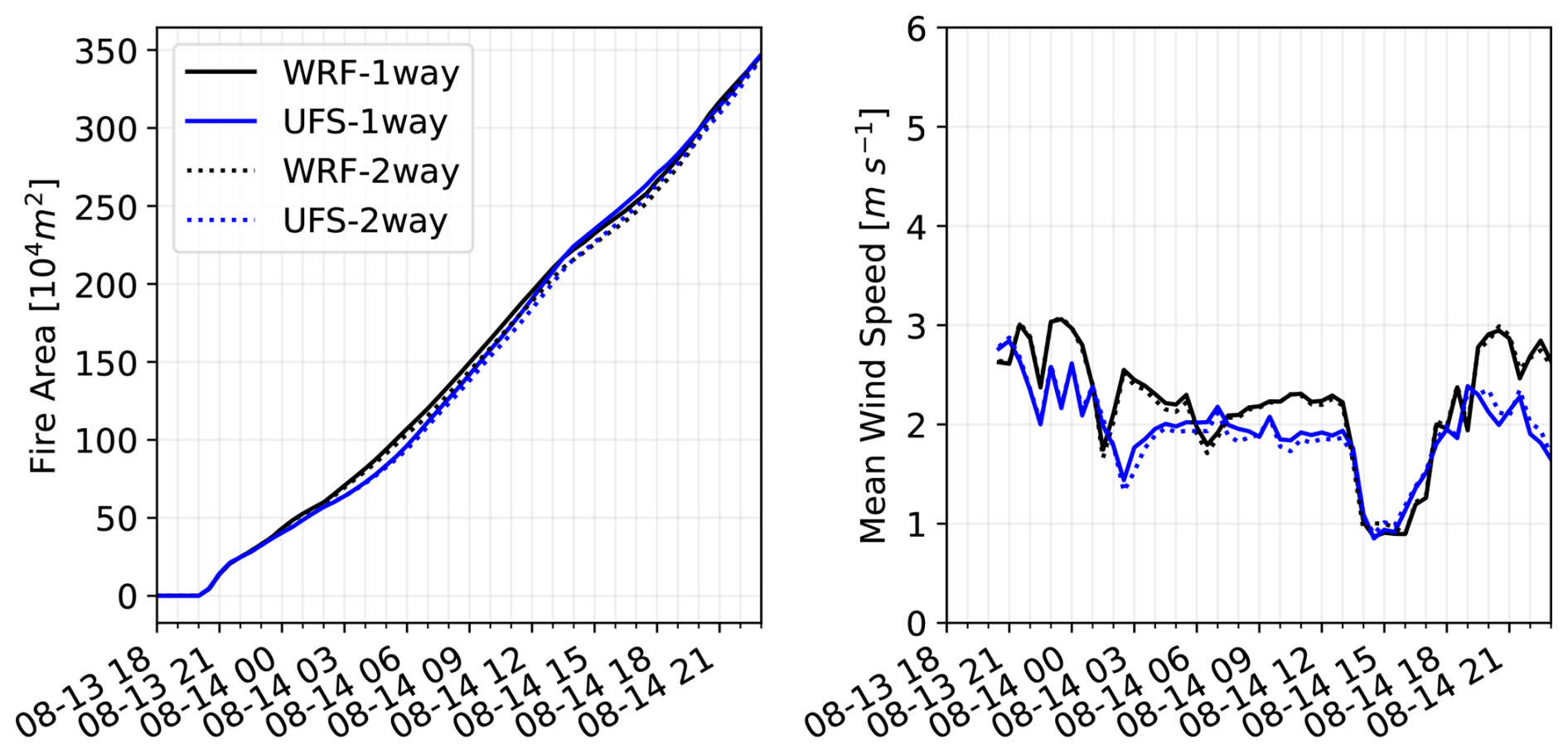
Figure 9 Same as Fig. 5 but including both one-way and two-way coupled fire–atmosphere simulations with WRF and UFS.

The overall consistency is also evident in the time series of the fire heat and moisture fluxes, and the smoke emissions (Fig. 10). These are the variables that are passed from the fire to the atmosphere component. This figure confirms that the one-way and two-way simulations produce similar fire fluxes at this grid spacing. There are some alternating peaks between the fluxes from WRF and UFS, but the fluxes from both models show similar overall lower frequency variability which is what would be expected given the similar configuration of the atmospheric models and the methods used in the fire behavior models.

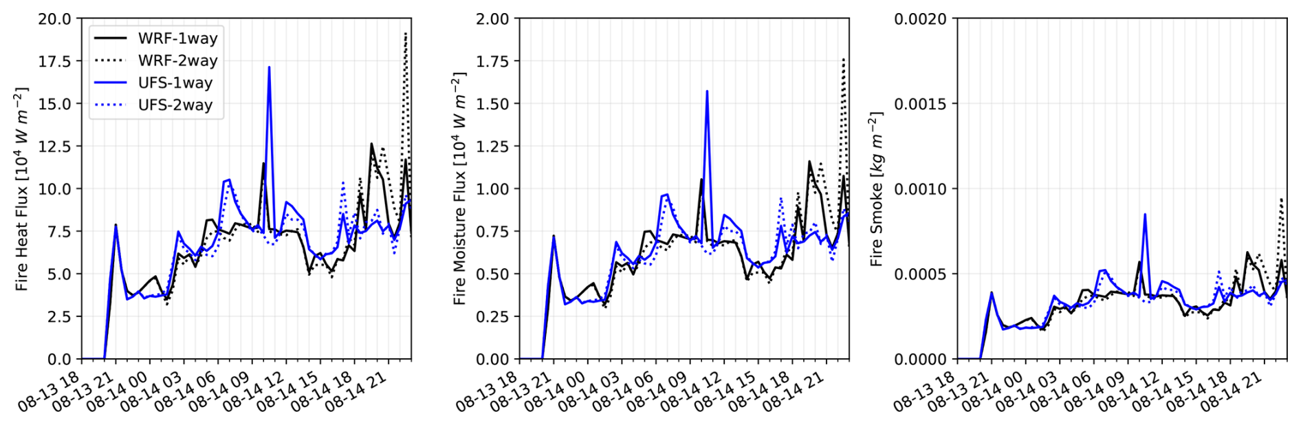
Figure 10 Time series of the fire heat flux (left), moisture flux (center), and smoke emissions (right).

The consistency of the fluxes passed to the atmospheric component are illustrated with the differences in the heat fluxes calculated with the two way and one way experiments using WRF and UFS shown in Fig. 11. The WRF differences are positive because WRF has dedicated variables for the fire fluxes in the atmospheric grid, with values set to zero in one-way experiments. However, UFS does not have dedicated variables for the fire fluxes in the atmospheric grid. The fire fluxes are incorporated into the heat and moisture fluxes at the surface. As a consequence, UFS differences sometimes can also be negative. However, at the location of the fire both models show positive differences of similar magnitude, with the UFS impact spread across more grid cells, at the three times shown.

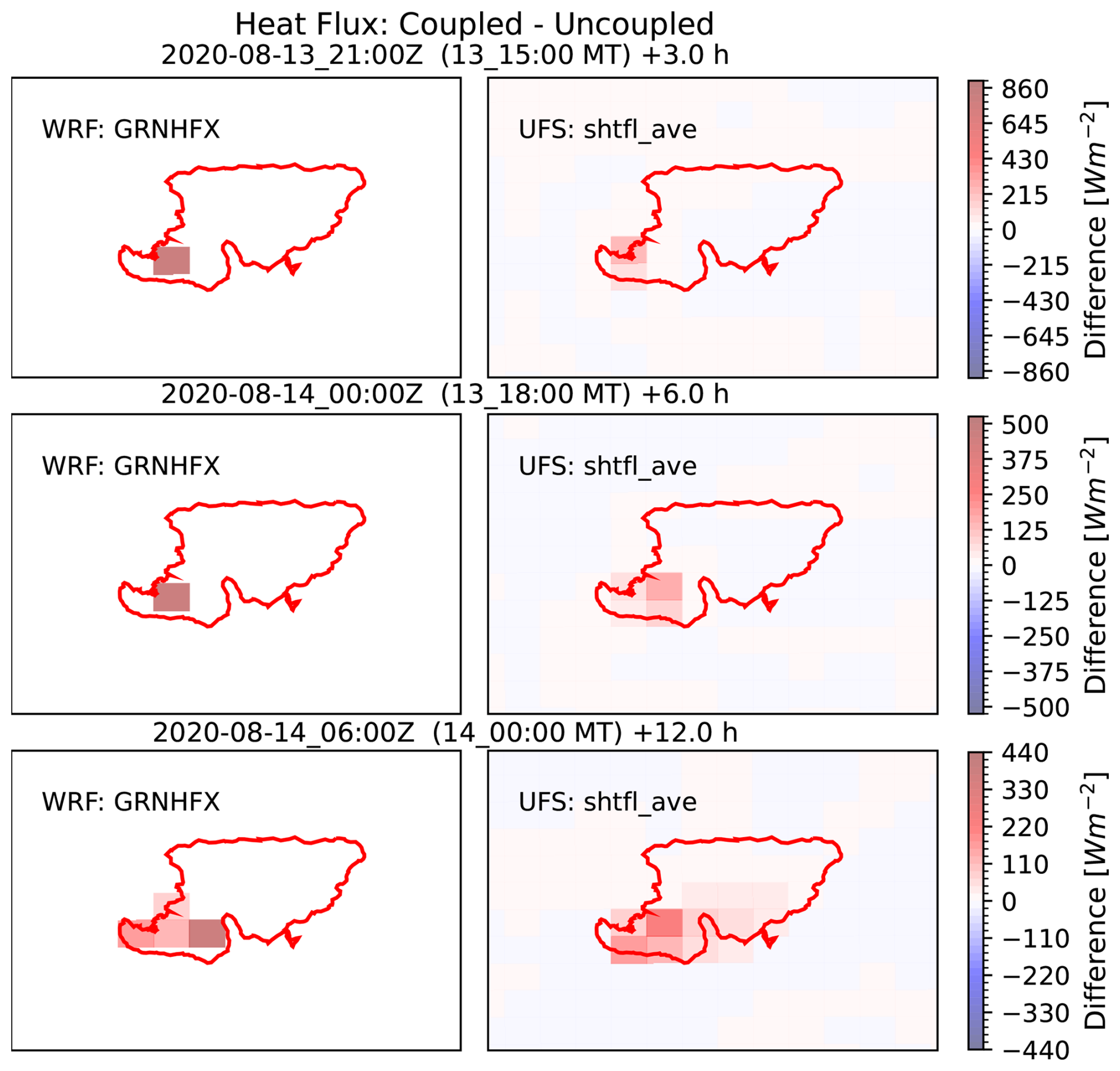
Figure 11 Fire heat flux differences between two-way and one-way simulations using the WRF model (left column) and the UFS model (right column) at 3 h (top row), 6 h (middle row), and 12 h (bottom row) into the simulations. To illustrate the location of the fire we also show Perimeter 3 valid for 14 August, 22:16 UTC (red solid line).

To conclude our analysis of the two way experiments, in Figs. 12, 13, and 14 we show the impacts of the fire fluxes in the first model vertical layer temperature, moisture, and vertical velocity, respectively. Outside of the active fire area, there is a mix of positive and negative differences without a clear pattern. However, the temperature shows positive values over the active fire region, increasing with lead time. The water vapor at the first model layer shows a smaller response to the fire moisture flux and no noticeable differences between the two way and one way simulation are seen as revealed by the near zero differences. For the case of the vertical velocity, there is not a noticeable difference in the first hours of the simulation, but, 12 h into the simulation when the fire grows in size, there is an increase in the vertical velocity as a result of the heat flux from the fire. Both models, WRF and UFS, show consistency in the spatial patterns of the differences.

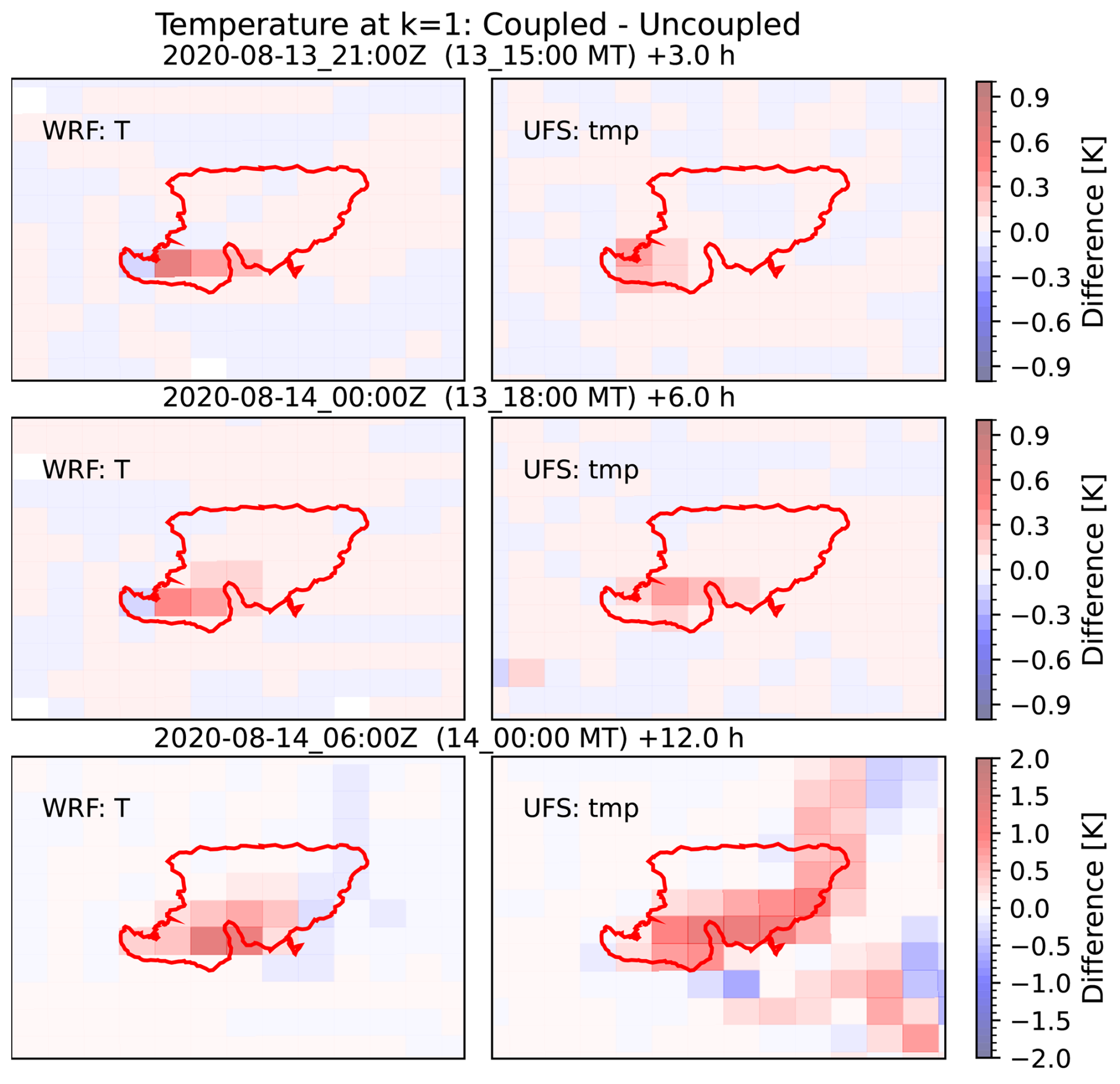
Figure 12 Same as Fig. 11 but for the temperature at the first model layer.

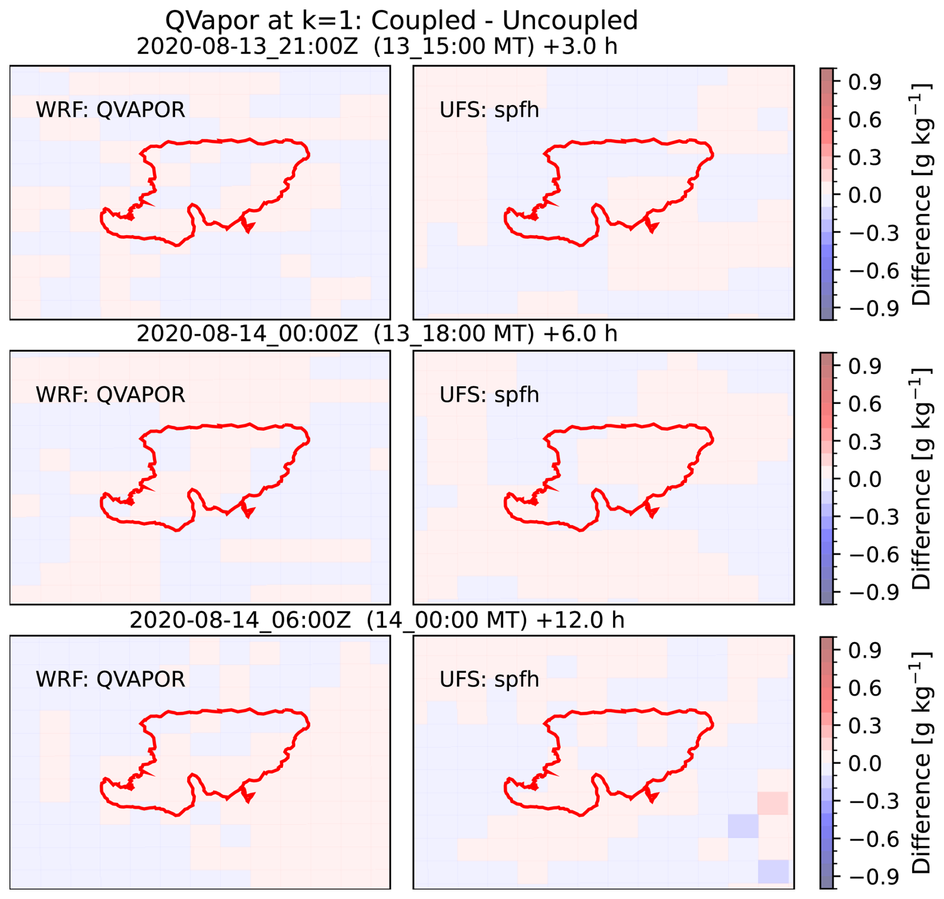
Figure 13 Same as Fig. 11 but for the water vapor mixing ratio at the first model layer.

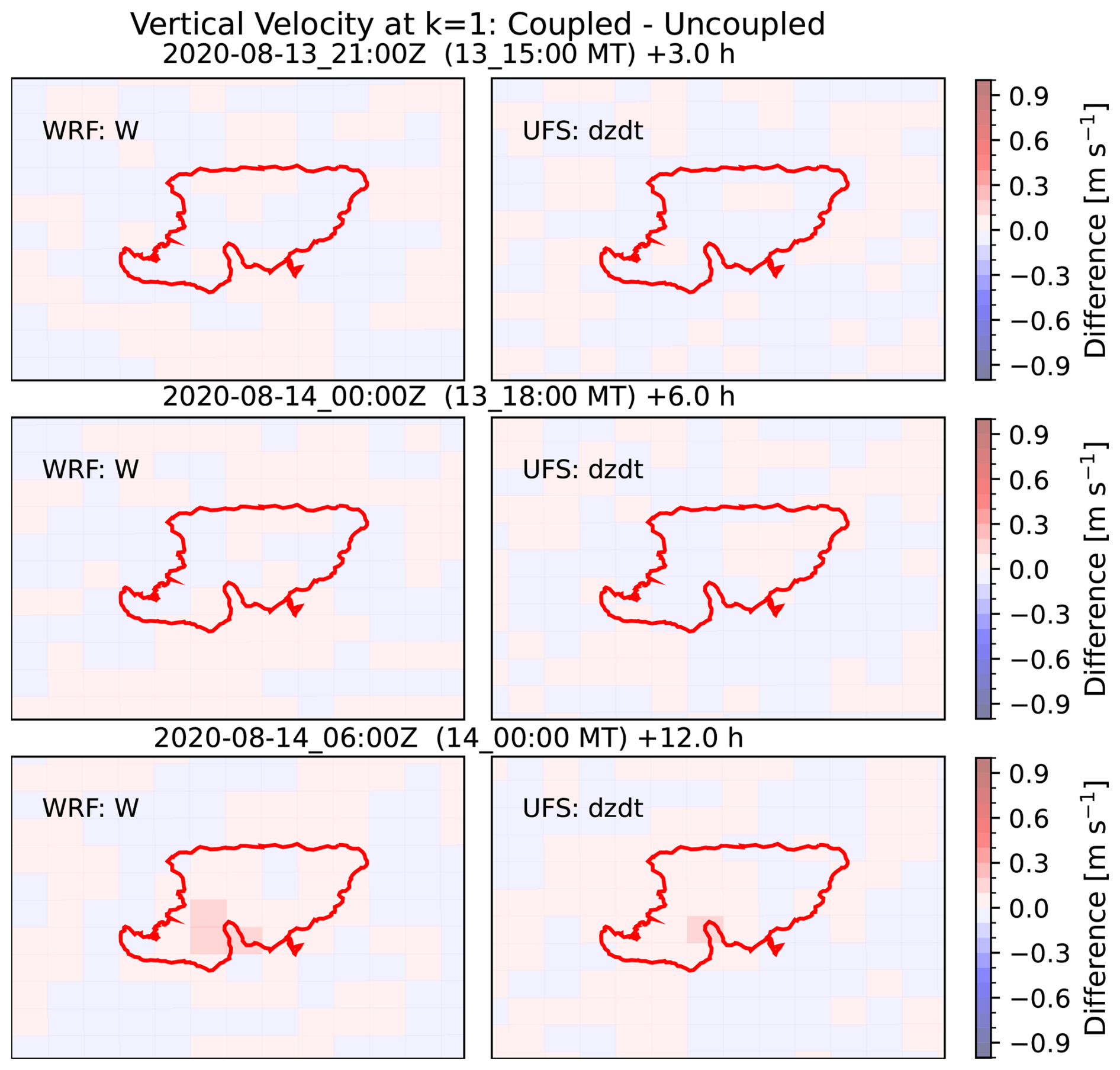
Figure 14 Same as Fig. 11 but for the vertical velocity at the first model layer.

4.2.4 Ignitions from observed perimeters for the Cameron Peak Fire

The comparison of the simulated fire perimeters for those experiments starting from Perimeter-1 or Perimeter-2 is shown in Fig. 15. For the experiments starting from Perimeter-1 (WRF-P1, UFS-P1, and CFB-P1) the fire mostly grows toward the northeast and southwest (Fig. 15 top). There is a general overprediction of the fire growth with respect to the CO-WIMS observations in certain portions of the perimeter. The overprediction seems to be a result of the fire perimeter not being active at the time of ignition as revealed by the similar observed perimeters in these regions at the beginning of the simulation and at the time shown (gray and red lines). If this is not the case, the discrepancies likely arise as misrepresentations of the winds in these portions of the perimeter. However, the three simulations, WRF-P1, UFS-P1, and CFBM-P1, are in good agreement in the northeast portion of the perimeter. Near the southwestern side of the perimeter, UFS-P1, and CFBM-P1 are in remarkably good agreement with WRF-P1 simulation a bit behind. This produces high Heidke skill scores between UFS and WRF-Fire, 0.95 or higher (Fig. 6), which highlights the consistency of the simulated fire perimeters between the two models.

The simulations starting from Perimeter-2 are also consistent with each other (Fig. 15 bottom). The three simulations (WRF-P2, UFS-P2, and CFB-P2) show remarkably good agreement. Indeed, the Heidke skill score comparing the perimeters from UFS-P2 and WRF-P2 is around 0.95 (Fig. 6). There is good agreement with observations in the western half of the perimeter. However, there is an overestimation in the southeastern part of the perimeter which is a result of misrepresentations of fuel barriers in the area, e.g. Highway 14 and Wright Creek, which run in parallel with the southeast portion of Perimeter-3 (red line) in this part of the fire front. To the northeast, the rate of spread of the fire is underestimated which is the opposite of what we found in this portion of the perimeter in the simulations starting from Perimeter-1 (Fig. 15 top). This could be attributed to timing errors in the simulation of the wind field, or inaccuracies in the timestamps of the observed perimeters.

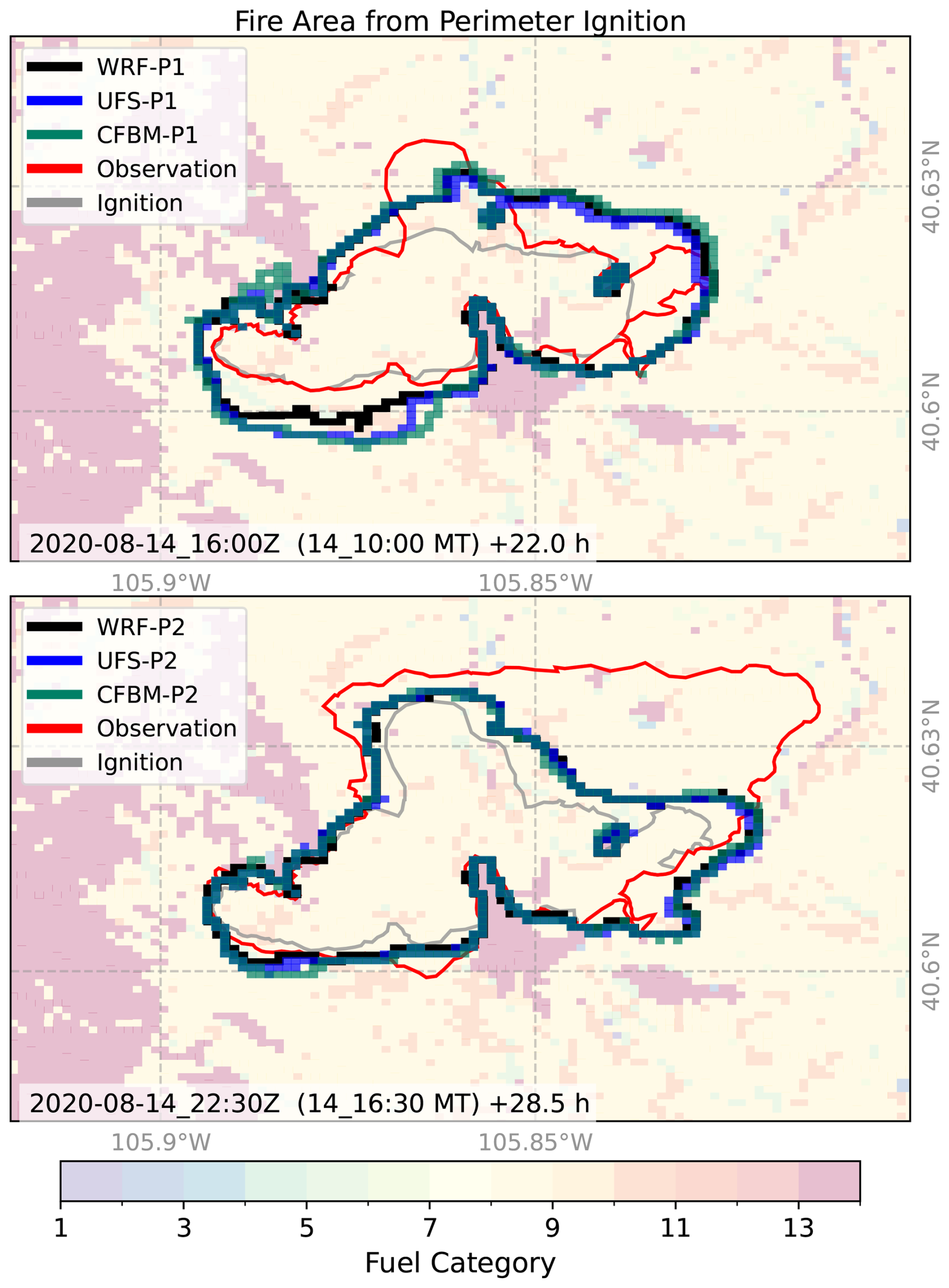
Figure 15 Simulated perimeters for the WRF-P1, UFS-P1, and CFB-P1 experiments at the time of the observed Perimeter-2 (top) as well as the simulated perimeters for the WRF-P2, UFS-P2, and CFB-P2 experiments at the time of the observed Perimeter-3 (bottom). The observed perimeters at the beginning of the simulations (gray line) and at the valid time of the simulations are also shown (red line).

5 Conclusions

In this study we present the CFBM, which, at its core in its current version 0.2.0, is a redesigned implementation of WRF-Fire 4.3.3 procedures in a new model available for coupling with atmospheric models through the ESMF library. The use of the ESMF library minimizes the source code needed to interpolate variables between the atmospheric and fire grids, and the synchronization and exchange of data between the atmosphere and the fire components. The fire behavior model is available as a NUOPC component and thus follows ESMF standards to integrate with other Earth system components. The CFBM is the first fire behavior model available for coupling via the ESMF library. Coupling to already existing Earth system's models where the atmospheric model is available as a NUOPC component should be straightforward. In its simplest configuration, the atmospheric model passes the winds and the roughness length to propagate the fires (one-way coupling). If the evolution of the ground FMC is simulated, then other standard surface variables (pressure, temperature, humidity, and precipitation) are used by the fire model. In addition, the fire behavior model can provide feedback to the atmosphere via sensible heat and latent heat fluxes, and smoke emissions (two-way coupling). This configuration requires connecting the heat/moisture fluxes to the atmospheric tendencies in the atmospheric model to modify the atmospheric evolution which in turn affects the winds and the fire evolution by accounting for fire–atmosphere interactions. Smoke emissions simulated as a fraction of the fuel burned at the ground are also available to the atmospheric component for coupling with radiation and cloud processes if desired.

In order to facilitate the evaluation of the CFBM NUOPC component, we closely followed WRF-Fire version 4.3.3 methods in the CFBM version 0.2.0. This allows for comparing CFBM simulations with an atmospheric host to WRF-Fire, a widely used fire behavior model. In spite of following WRF methods, substantial changes have been introduced in the code to create a fire model independent of the atmospheric component which also allows for ESMF coupling, improved performance, and readability, as well as facilitating maintenance and extension of the code. The model can be also run in standalone mode using data from an existing WRF simulation. This standalone version of the code does not require the ESMF library and can be used to test developments and sensitivities to the fire evolution.

The CFBM has been coupled to UFS, and this allowed us, for the first time, to perform fire behavior simulations with UFS. We then compared UFS simulations to WRF-Fire to ensure a proper development. Our results for the Cameron Peak Fire show consistency of the fire evolution simulated by the standalone model, UFS, and WRF-Fire (Fig. 6). Comparisons of one-way versus two-way fire simulations showed small impacts in the atmospheric evolution. This is mostly a consequence of the relatively coarse grid spacing used, 1 km, but it was sufficient to ensure consistency between UFS and WRF-Fire. The consistency between UFS and WRF-Fire is encouraging for the UFS community to start performing fundamental research on fire-weather interactions. This consistency is also the starting point for ongoing developments to improve the accuracy of the simulated fire evolution beyond the original WRF-Fire model.

The CFBM is the first fire behavior model available for coupling with atmospheric models as a NUOPC component in ESMF. This is expected to facilitate its adoption by other atmospheric models, especially those already using the ESMF library. In this way, the fire community can benefit from having the same modeling framework. We also envision that our efforts may pave the way for future fire model intercomparison efforts, a common practice in various atmospheric science modeling communities. Indeed, our vision is to foster collaborative development in fire behavior modeling with the ultimate goal of increasing our fundamental understanding of fire science and minimizing the adverse impacts of wildland fires.