RTSEvo v1.0: a retrogressive thaw slump evolution model

Widespread thermal degradation in permafrost regions is accelerating the development of retrogressive thaw slumps (RTS), severely threatening ecological stability and critical infrastructure. Current RTS modeling efforts, however, are largely confined to static susceptibility mapping, lacking the capacity to predict their spatiotemporal evolution. To bridge this gap, we developed RTSEvo, a novel dynamic RTS evolution model that couples three modules: (1) a time-series forecast of regional RTS area demand, (2) a machine-learning module for pixel-level probability mapping, and (3) a physically constrained spatial allocation module that simulates RTS expansion by integrating neighborhood effects, stochasticity, and a novel retrogressive erosion factor. Validated using manually interpreted RTS maps for 2021 and 2022 in the Beiluhe Basin on the Qinghai-Tibet Plateau, the model successfully simulated dynamic RTS growth, with the Logistic Regression-based model showing superior stability and accuracy. Furthermore, cross-regional validation confirmed the framework's structural generalizability. An interesting finding is that predictive skill is significantly enhanced by integrating process-based rules with statistical probability. Specifically, the inclusion of the retrogressive erosion factor, which mechanistically simulates upslope headwall retreat, proved critical, improving model performance by up to 29.3 % as measured by the Figure of Merit. The primary innovation of this study is the successful realization of a regional-scale dynamic simulation and prediction of RTS expansion. RTSEvo offers a highly robust scientific tool for informing proactive RTS-related risk mitigation strategies.

1 Introduction

Permafrost, defined as ground that remains at or below 0 °C for at least two consecutive years, is a critical component of the cryosphere that underlies approximately 15 % of the Northern Hemisphere's exposed land area (Obu, 2021). The Qinghai-Tibet Plateau (QTP) hosts the most extensive permafrost terrain in the world's low to mid-latitudes and is a recognized hotspot of climate sensitivity (Cheng et al., 2019; Yao et al., 2019; Zhao et al., 2024). In recent decades, the QTP has warmed at more than twice the global average rate (Kuang and Jiao, 2016; Zhang et al., 2021), triggering widespread permafrost degradation. This degradation is evidenced by rising ground temperatures, a deepening active layer, and a reduction in permafrost extent (Zhang et al., 2022; Ran et al., 2018). The rate of active layer thickening, for instance, has accelerated to an estimated 46.7±26.9 cm per decade (Ziteng et al., 2025).

A prominent and destructive consequence of the rapid thawing of ice-rich permafrost is the proliferation of thermokarst hazards, particularly retrogressive thaw slumps (RTSs) (Maier et al., 2025a). An RTS is a form of slope failure characterized by a steep, retreating headwall where exposed ground ice melts, leading to the downslope movement of a slurry of thawed sediment and water. The spatiotemporal footprint of these features across the QTP is expanding dramatically, with the total area of RTS increasing more than 26-fold since 1986 (Yang et al., 2023). These disturbances not only threaten the stability of alpine ecosystems (Lantz et al., 2009) and the safety of critical infrastructure (Niu et al., 2005; Hjort et al., 2022) but also mobilize large quantities of previously frozen organic carbon (Mu et al., 2016; Cassidy et al., 2017), creating a positive feedback loop to global climate change (Zhou et al., 2023).

The development of RTS is governed by a complex interplay of environmental controls. They typically form on gentle slopes in areas of warm permafrost (mean annual ground temperature > −1 °C) with high ground ice content. While climate warming and heavy precipitation are primary drivers that reduce slope stability (Luo et al., 2024b), local factors such as engineering disturbances and thermal erosion also play a crucial role (Li et al., 2024; Jin et al., 2005; Luo et al., 2022a). To identify high-risk areas, many recent studies have successfully applied machine learning algorithms such as random forests (RF) and generalized linear models (GLM) to produce static susceptibility maps (Yin et al., 2021, 2023; Wang et al., 2024; Rudy et al., 2016).

However, these susceptibility assessments have a fundamental limitation: they provide a static snapshot of risk based on a set of conditioning factors, but they cannot capture the inherently dynamic evolution of RTSs. The expansion of an RTS is not merely a probabilistic occurrence but a process-driven phenomenon characterized by positive feedback mechanisms, such as the continuous exposure of ice at the headwall (Deng et al., 2024; Lewkowicz and Way, 2019), which accelerates retreat. Static models lack the capacity to simulate this temporal progression or predict how RTS fields will evolve under future climate scenarios.

To address this gap, we draw inspiration from the well-established field of Land Use and Land Cover Change (LUCC) modeling. For decades, LUCC models have been developed to simulate the spatiotemporal dynamics of landscape change by coupling a macro-scale projection of change with a spatially explicit allocation module (Verburg et al., 2002; Verburg and Overmars, 2009). This framework is well-suited for modeling process-driven phenomena because the allocation of new cells is governed by transition rules that can encode underlying physical processes. For example, the common use of neighborhood effect in LUCC models is a simple but powerful way to represent the positive feedback and spatial contagion characteristic of RTS expansion. This flexible structure allows for the integration of more sophisticated, physically-based rules that can guide the simulation. This methodological paradigm, which combines statistical probabilities with process-driven spatial rules, therefore offers a promising foundation for dynamically modeling RTS evolution.

Building on this approach, we developed an innovative dynamic evolution model for RTS (RTSEvo). This framework moves beyond static susceptibility by coupling three core modules: (1) a time-series forecasting module to project the total regional RTS area demand; (2) a machine learning module to generate a baseline pixel-level occurrence probability based on environmental drivers; and (3) a constrained spatial allocation module that simulates RTS expansion by integrating the occurrence probability with neighborhood effects, a retrogressive erosion factor, and stochasticity, ensuring the total simulated area matches the projected demand. By explicitly modeling spatial propagation and temporal growth, our approach aims to provide a more realistic and predictive tool for regional disaster risk assessment and management under a changing climate.

2 Material and methods

2.1 The RTS evolution model framework

Our model (RTSEvo v1.0) simulates RTS evolution by discretizing the landscape into a grid of cells (pixels). Unlike LUCC models that often manage transitions among multiple land cover types, our model simplifies the system to a binary classification. Each cell exists in one of two states: non-RTS (value = 0) or RTS (value = 1). This focus allows the framework to concentrate on the irreversible transition of cells from a non-RTS to an RTS state over annual time steps. This state transition is governed by a modular framework designed to integrate regional-scale trends with local-scale drivers (Fig. 1).

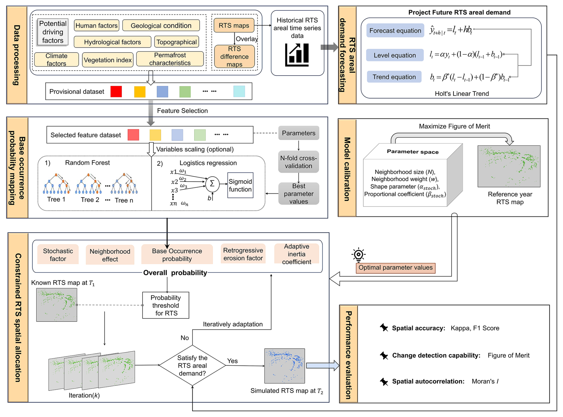
Figure 1 Conceptual framework and workflow of the dynamic retrogressive thaw slump (RTS) evolution model. The workflow begins with processing multi-source data to train the models. It consists of three interlinked modules: (1) areal demand forecasting, which uses Holt's linear trend model to project the total RTS area serving as a macro-scale constraint; (2) base occurrence probability mapping, which employs machine learning algorithms (Random Forest or Logistic Regression) to generate a pixel-level probability map for RTS initiation; and (3) constrained spatial allocation, which dynamically allocates new RTS pixels by integrating the base probability with neighborhood effects, a retrogressive erosion factor, a stochastic factor, and an adaptive inertia coefficient until the projected area demand is met. Model parameters are optimized through a calibration process that maximizes the Figure of Merit (FoM), and final performance is evaluated using FoM, κ, F₁ Score and Moran's I.

The framework consists of three core, interlinked modules. (1) RTS areal demand forecasting module: This module projects the total RTS area for the target year, establishing a top-down, macro-scale constraint on overall RTS expansion. (2) Base occurrence probability mapping module: This module uses machine learning to calculate the baseline probability of RTS initiation for each individual pixel based on its unique environmental characteristics (e.g., topography, climate, geology). (3) Constrained spatial allocation module: This module serves as the dynamic engine of the model. It iteratively allocates new RTS cells on the landscape by combining the base occurrence probability with spatial interaction rules (neighborhood and retrogressive erosion effects) until the estimated total area demand is met.

The model is calibrated using a historical RTS distribution map from a reference year. The optimal model parameters are determined by systematically tuning them to maximize the agreement between the simulated and observed RTS patterns from that reference year.

2.2 Module 1: RTS areal demand forecasting

A key constraint for the simulation is the total new area of RTS to be allocated in a given year. To prevent uncontrolled expansion, we first forecast this regional demand. We employed Holt's linear trend method, an exponential smoothing technique well-suited for time-series data exhibiting a clear trend (Holt, 2004), which has been observed for RTS growth on the QTP since 2011 (Maier et al., 2025b). The method uses a level equation (current magnitude), a trend equation (rate of change), and a forecast equation:

$$\begin{array}{}\text{(1)}& \left\{\begin{array}{ll}\mathrm{Level}\mathrm{equation}:& l_t=a{y}_t+(\mathrm{1}-a)\left(l_{t-\mathrm{1}}+b_{t-\mathrm{1}}\right)\\ \mathrm{Trend}\mathrm{equation}:& b_t={\mathit{\beta }}^{*}\left(l_t-l_{t-\mathrm{1}}\right)+\left(\mathrm{1}-{\mathit{\beta }}^{*}\right)b_{t-\mathrm{1}}\\ \mathrm{Forecast}\mathrm{equation}:& {\widehat{y}}_{(t+h\mathrm{|}t)}=l_t+h{b}_t\end{array}\right.\end{array}$$

where l_t is the estimated level (baseline area) at time t, b_t is the estimated trend (growth rate), y_t is the observed area at time t, and ${\widehat{y}}_{(t+h\mathrm{|}t)}$ is the forecasted area for h time steps into the future. The smoothing parameters for level (α) and trend (β^*) range from 0 to 1 and control the weighting of recent versus past observations.

2.3 Module 2: base occurrence probability mapping

This module quantifies the intrinsic suitability of each pixel for RTS formation based on a suite of environmental driving factors, independent of its spatial context. We tested two widely used machine learning algorithms for this task: Logistic Regression (LR) and Random Forest (RF).

LR is a generalized linear model that calculates the probability of an outcome using the sigmoid function, providing a clear, interpretable relationship between the drivers and RTS occurrence (Cramer, 2003). The probability P_i for pixel i is given by:

$$\begin{array}{}\text{(2)}& P_i\left({\mathit{X}}^i\right)={\displaystyle \frac{\mathrm{1}}{\left(\mathrm{1}+e^{(-z)}\right)}}\end{array}$$

where Xⁱ represents the feature vector for a single pixel i, containing the values of all environmental driving factors for that specific pixel, and $z=w_{\mathrm{1}}{x}_{\mathrm{1}}^i+w_{\mathrm{2}}{x}_{\mathrm{2}}^i+\mathrm{\dots }+w_n{x}_n^i+b$, is the linear combination of weighted predictor variables. w represents the weights associated with each predictor variable, and b is the bias term.

RF is an ensemble learning algorithm that builds a multitude of decision trees and aggregates their outputs. It is robust to non-linear relationships and interactions between variables. The probability is calculated as the proportion of trees in the forest that classify the pixel as an RTS (Breiman, 2001; Sun et al., 2021):

$$\begin{array}{}\text{(3)}& P_i\left({\mathit{X}}^i\right)={\displaystyle \frac{\sum _{n=\mathrm{1}}^{{\mathrm{Tree}}_{\mathrm{total}}}\mathrm{1}\left({\mathrm{Tree}}_n\left({\mathit{X}}^i\right)=\mathrm{1}\right)}{{\mathrm{Tree}}_{\mathrm{total}}}}\end{array}$$

where 1(⋅) is the indicator function and Tree_total is the total number of trees in the forest. Tree_n(Xⁱ) refers to the prediction from a single decision tree within the RF, i.e., the output of the nth tree when it is given the feature vector Xⁱ as input.

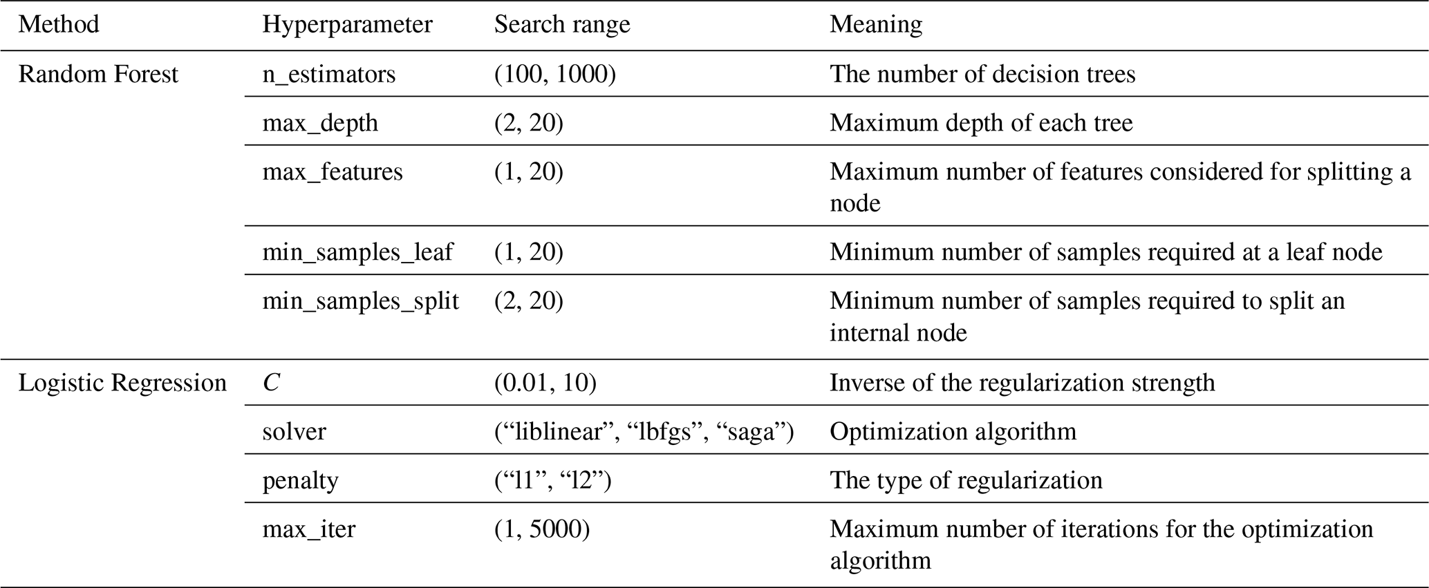
The performance of machine learning models is highly dependent on the selection of their hyperparameters, which are settings that control the learning process itself (Probst et al., 2019). To find the optimal configuration for both the RF and LR models, we implemented a systematic tuning process. While traditional methods like Grid Search and Randomized Grid Search are common, they can be computationally inefficient, especially with many parameters. Therefore, we employed Latin Hypercube Sampling (LHS), a more advanced statistical method for parameter optimization. LHS is superior because it explores the parameter space more efficiently by dividing each parameter's range into equal intervals and sampling exactly one value from each interval, ensuring a more uniform and representative coverage with fewer trials (McKay et al., 1979). We first defined a plausible search range for each key hyperparameter in the RF and LR models (Table 1). For RF, this included parameters like the number of trees (n_estimators) and maximum tree depth (max_depth); for LR, it included regularization strength (C) and the optimization algorithm (solver). LHS was used to generate 100 unique combinations of hyperparameters from these ranges. Then each parameter combination was evaluated using 10-fold cross-validation accuracy as the objective function. The hyperparameter combination that resulted in the highest average cross-validation accuracy was selected as the optimal configuration for the final model used for base occurrence probability mapping.

Table 1 Hyperparameter search ranges for the Random Forest (RF) and Logistic Regression (LR) models. These ranges were systematically explored using Latin Hypercube Sampling to determine the optimal parameter combination for the base occurrence probability mapping.

2.4 Module 3: constrained RTS spatial allocation

This module transforms the static probability map from Module 2 into a dynamic RTS distribution that adheres to the area demand from Module 1. This is achieved through an iterative process within a cellular automata framework (Wolfram, 1983; Toffoli and Margolus, 1987). At each iteration k, a total transition probability ($P_{\mathrm{Total},i}^k$) is calculated for every non-RTS cell, integrating the base probability with four dynamic factors:

$$\begin{array}{}\text{(4)}& P_{\mathrm{Total},i}^k=P_i\times U_i^k\times {\mathrm{Erosion}}_i^k\times R{A}_i^k\times {\mathrm{Inertia}}_i^k\end{array}$$

where P_i is the base occurrence probability representing the intrinsic suitability of pixel i, as calculated in Module 2; $U_i^k$ represents the neighborhood effect that accounts for spatial autocorrelation, based on the principle that a new RTS is more likely to form near existing ones; Erosion${}_i^k$ is a retrogressive erosion factor, a novel component designed to mimic the characteristic upslope (headward) retreat of RTS; $R{A}_i^k$ is a stochastic factor designed to simulate the inherent randomness and unmodeled variables in natural systems; and Inertia${}_i^k$ denotes an adaptive inertia coefficient serving as a dynamic regulator that accelerates or decelerates the overall rate of new RTS allocation to ensure the final simulated area matches the target area demand from Module 1.

The neighborhood effect factor is calculated as the density of RTS cells within a defined neighborhood window:

$$\begin{array}{}\text{(5)}& U_i^k={\displaystyle \frac{\sum _{N\times N}\mathrm{1}\left(s_i^{k-\mathrm{1}}=\mathrm{1}\right)}{N\times N-\mathrm{1}}}\times w\end{array}$$

where the numerator counts RTS cells in an N×N window at the previous iteration (k−1) and w is a weight factor. $\mathrm{1}(s_i^{k-\mathrm{1}}=\mathrm{1})$ is an indicator function that counts how many neighboring cells are already in the RTS state (s=1).

The retrogressive erosion factor assigns a higher probability weight to cells located in the direction opposite to the local slope aspect (Luo et al., 2024a), thereby promoting directional growth. The directional weight (w_mn) is calculated based on the angular difference (Δθ) between the potential growth direction and the theoretical erosion direction (θ_erosion), which is 180° from the slope aspect, representing how closely its direction aligns with the ideal erosion path. The equations are given as follows:

$$\begin{array}{}\text{(6)}& \left\{\begin{array}{l}{\mathit{\theta }}_{\mathrm{erosion}}=\left({\mathit{\theta }}_{\mathrm{aspect}}+\mathrm{180}\mathit{°}\right)\mathrm{mod}\mathrm{360}\mathit{°}\\ {\mathit{\theta }}_{mn\to ij}=\arctan \mathrm{2}(i-m,n-j)\mathrm{mod}\mathrm{360}\mathit{°}\\ \mathrm{\Delta }\mathit{\theta }=\min \left(\mathrm{|}{\mathit{\theta }}_{mn\to ij}-{\mathit{\theta }}_{\mathrm{erosion}}\mathrm{|},\mathrm{360}\mathit{°}-\mathrm{|}{\mathit{\theta }}_{mn\to ij}-{\mathit{\theta }}_{\mathrm{erosion}}\mathrm{|}\right)\\ w_{mn}=\cos (\mathrm{\Delta }\mathit{\theta }/\mathrm{2})\\ {\mathrm{Erosion}}_i^k=\frac{\sum _{N\times N}{w}_{mn}\times \mathrm{1}\left(s_{mn}^k=\mathrm{1}\right)}{\sum _{N\times N}{w}_{mn}}\end{array}\right.\end{array}$$

where θ_aspect is the standard slope aspect for the cell calculated from the digital elevation model (DEM), and θ_mn→ij is the azimuth angle from a central cell at coordinates (i, j) to each of its neighbors at coordinates (mn). 1(s_mn=1) is an indicator function (where state s=1). Erosion${}_i^k$ is thus calculated as a proportion of a numerator term that sums the directional weights (w_mn) of all neighboring cells that are currently in the RTS state, over a denominator that is the sum of the directional weights of all neighbors, regardless of their state.

The stochastic factor ($R{A}_i^t$) is based on an extreme value distribution (Coles, 2001; Davison and Huser, 2015):

$$\begin{array}{}\text{(7)}& R{A}_i^k=\mathrm{1}+{\mathit{\beta }}_{\mathrm{stoch}}\times \left((-\log R{)}^{{\mathit{\alpha }}_{\mathrm{stoch}}}-\mathrm{0.5}\right)\end{array}$$

where R is a random value between 0 and 1, and α_stoch and β_stoch control the shape and magnitude of the perturbation. The search range of α_stoch was set to (0.01, 0.5) for practical purposes, as this range ensures the introduction of moderate, plausible fluctuations without destabilizing the model. The range of β_stoch was set to (0.1, 1) which aims to balance the influence of randomness in the model.

The inertia coefficient is calculated by a piecewise function (Eq. 8). The core variable is D^k, which represents the difference between the number of simulated RTS cells and the required number (the demand) at iteration k.

$$\begin{array}{}\text{(8)}& {\mathrm{Inertia}}^k=\left\{\begin{array}{ll}{\mathrm{Inertia}}^{k-\mathrm{1}}& \mathrm{if}\left|D^{k-\mathrm{1}}\right|\le \left|D^{k-\mathrm{2}}\right|\\ {\mathrm{Inertia}}^{k-\mathrm{1}}\times \frac{D^{k-\mathrm{2}}}{D^{k-\mathrm{1}}}& \mathrm{if}{D}^{k-\mathrm{1}}<D^{k-\mathrm{2}}<\mathrm{0}\\ {\mathrm{Inertia}}^{k-\mathrm{1}}\times \frac{D^{k-\mathrm{1}}}{D^{k-\mathrm{2}}}& \mathrm{if}\mathrm{0}<D^{k-\mathrm{2}}<D^{k-\mathrm{1}}\end{array}\right.\end{array}$$

Once the total transition probability ($P_{\mathrm{Total},i}^k$) is calculated for each non-RTS cell, a probability threshold method is used to determine if a state change occurs. If $P_{\mathrm{Total},i}^k>P_{\mathrm{Threshold}}^k$, the cell's state transitions from non-RTS (0) to RTS (1). Crucially, this state transition is assumed to be irreversible; once a pixel converts to the RTS state, it remains in that state for all subsequent time steps of the simulation. This entire allocation process continues iteratively. The simulation for a given year concludes when the total area of simulated RTS cells meets the target demand projected by Module 1.

2.5 Model calibration

The Constrained Spatial Allocation module contains several key parameters (e.g., neighborhood size N, neighborhood weight w, stochastic shape parameters α_stoch and proportional coefficient β_stoch) that require calibration (Table 2). We implemented a systematic calibration procedure using LHS to efficiently sample the multi-dimensional parameter space. For each parameter set generated by LHS, the model was run to simulate the RTS distribution for a historical reference year. The performance of each run was evaluated by comparing the simulated map to the actual observed map using the Figure of Merit (FoM) metric, which measures the accuracy of change detection. The parameter set that yielded the highest FoM was selected as the optimal configuration for future simulations.

Table 2 Parameter search ranges and optimal values for the constrained RTS spatial allocation module.

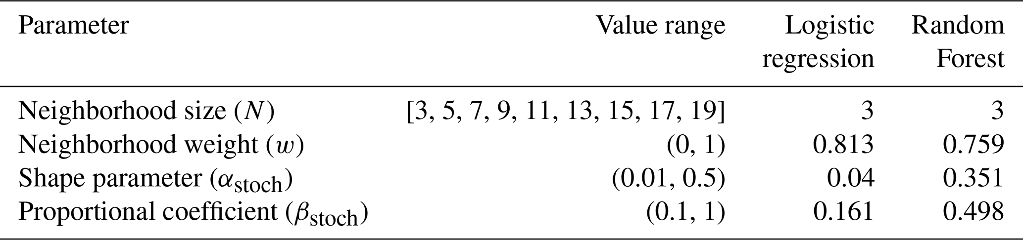
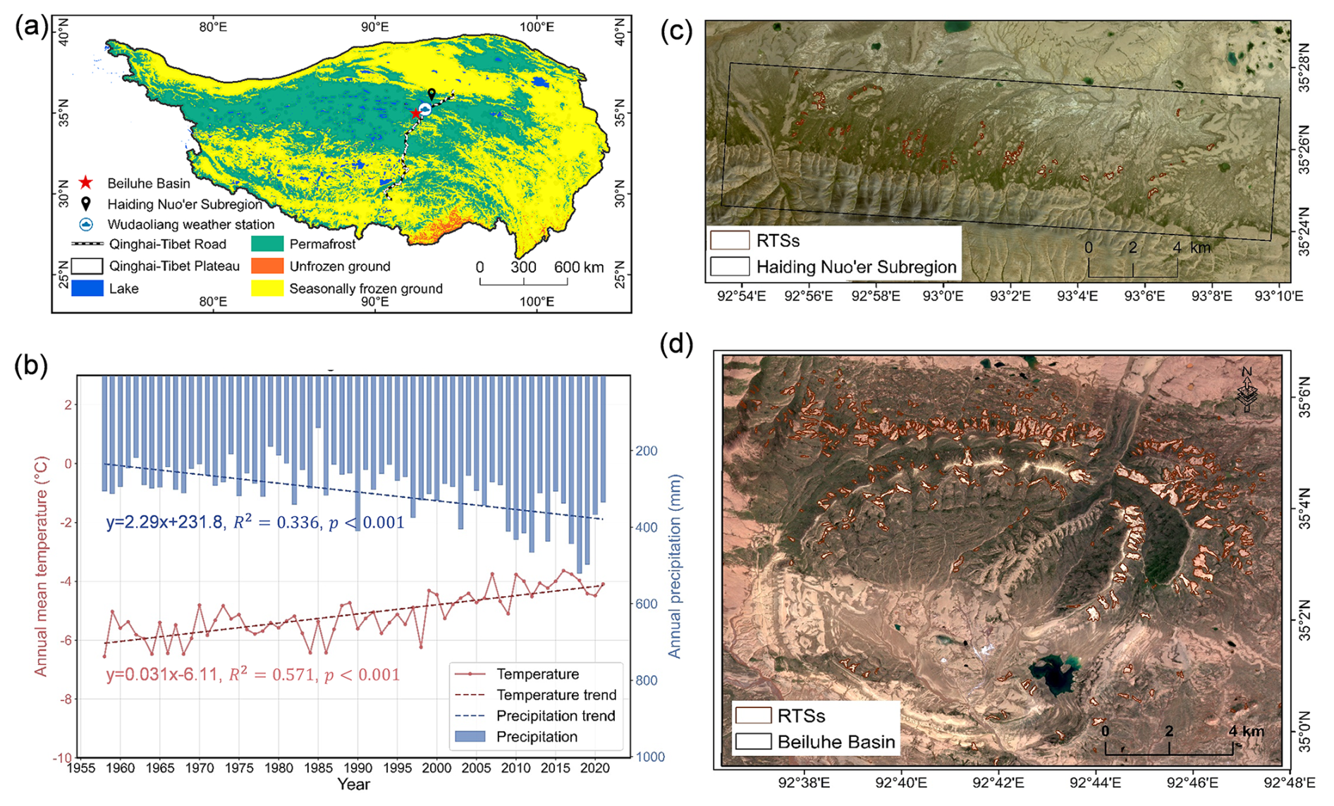
Figure 2 Location of the primary study area (Beiluhe Basin) and the transferability test region (Haiding Nuo'er Subregion), alongside regional climate trends and RTS distribution. (a) Permafrost distribution on the QTP, with the primary study area marked by a red star and the Haiding Nuo'er Subregion marked by a black pin. Permafrost data are from Cao et al. (2023). (b) Air temperature and precipitation records from the nearby Wudaoliang weather station (1955–2021), with trend lines illustrating regional warming and humidification. (c, d) 2022 PlanetScope satellite images (Planet Team, 2025) of the Haiding Nuo'er Subregion and the Beiluhe Basin, respectively, overlaid with mapped RTS boundaries from Xia et al. (2024a).

2.6 Case study application

2.6.1 Primary study area and transferability test region

We tested and validated our model primarily in the Beiluhe Basin, a region in the central QTP (Fig. 2d) that is a representative hotspot for permafrost degradation. Situated at an average elevation of over 4500 m, the basin is underlain by continuous, ice-rich permafrost, with volumetric ice content exceeding 25 % (Yin et al., 2017). The permafrost here is thermally sensitive, classified as warm with a mean annual ground temperature at 15 m depth ranging from −1.8 to −0.5 °C (Luo et al., 2015). The landscape is dominated by alpine meadows and alpine grasslands, which cover over 40 % of the regional land area (Yin et al., 2017). The local climate is cold and semi-arid; observations from the Wudaoliang meteorological station near the Beiluhe Basin, show a mean annual air temperature of −5.0 °C and mean annual precipitation of approximately 300 mm (Fig. 2b). Over 90 % of this precipitation is concentrated in the summer months (May to September), while annual evaporation exceeds 1000 mm. Since 1960, the region has experienced a significant warming and humidification trend, with an accelerated rate of increase in both temperature and precipitation after 2000 (Yu et al., 2025). The combination of climate change, topography, and vulnerable permafrost has resulted in the formation of over 450 documented RTS features (Xia et al., 2024b), making it an ideal primary study area.

To independently validate model transferability, the Haiding Nuo'er Subregion (extending from 92.889 to 93.167° E and from 35.396 to 35.469° N) is introduced as a secondary test region (Fig. 2c). The Haiding Nuo'er Subregion is characterized by alpine meadow and alpine grassland ecosystems, similar in general land cover to the Beiluhe Basin, but it exhibits distinct environmental conditions. The number of mapped RTS features in this region increased from 52 to 92 between 2016 and 2022, indicating active thermokarst development. Compared to the Beiluhe Basin, RTS occurrences in the Haiding Nuo'er Subregion are associated with lower elevations and reduced vegetation greenness, as well as higher silt content in the 30–60 cm soil layer and greater thawing degree days (Fig. S1 in the Supplement). These differences reflect variations in topographic setting, surface conditions, soil composition, and thermal forcing, which are key controls on permafrost stability and RTS initiation. Such differences provide a valuable opportunity to examine the model's applicability and generalizability under varying environmental controls.

2.6.2 Data acquisition and preparation

The ground-truth data for this study consisted of annual RTS inventories for both the Beiluhe Basin and the Haiding Nuo'er Subregion from 2016 to 2022. Over this period, more than 200 new RTS were identified, covering a cumulative area of 1042.47 ha (Xia et al., 2024b). Individual slump areas ranged from 0.11 to 22.39 ha, with an average of 2.61 ha (Luo et al., 2022b). For the Haiding Nuo'er Subregion, the corresponding annual inventories captured the active expansion of these features over the same timeframe. These inventories were derived from the manual interpretation of high-resolution (3 m) PlanetScope imagery acquired in August of each year; their high reliability was confirmed by a low relative area error of 4.6 % when compared against field-mapped boundaries (Xia et al., 2024b). Because August marks the end of the summer thaw season, the resulting maps are assumed to represent the full extent of RTS activity for the annual cycle spanning from September of the preceding year to August of the current year.

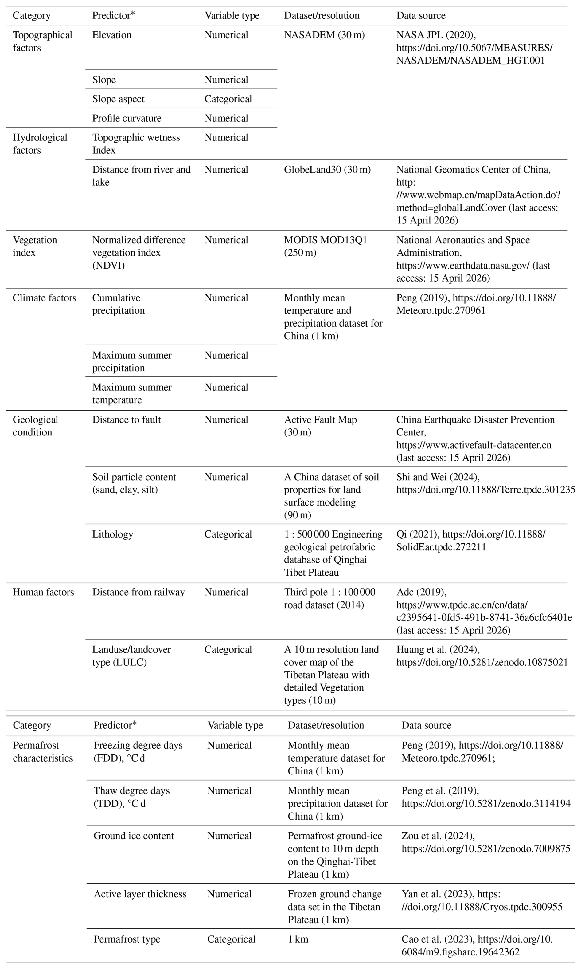
For the explanatory variables, a comprehensive set of 36 potential driving factors was initially compiled (Table A1), spanning six categories: topography, climate, geology, hydrology and vegetation, permafrost characteristics, and human activities (Rudy et al., 2016; He et al., 2024; Lacelle et al., 2009; Kokelj et al., 2015; Yin et al., 2023). The suitability of the remaining factors was validated using non-parametric tests to assess differences between RTS and non-RTS groups. The Mann–Whitney U test was applied to numerical data and the χ² test to categorical data. The results confirmed that all but one factor (clay content at 100–200 cm depth) showed a statistically significant difference (p<0.01), supporting their inclusion as potential predictors (Figs. A1 and A2). In particular, the active layer thickness (ALT) exhibits a clear bimodal distribution (Fig. A2). The bimodal distribution reflects the presence of two dominant ground thermal regimes in the Beiluhe Basin. Continuous vegetation and organic layers maintain a shallow active layer through strong thermal insulation, whereas RTS-affected surfaces experience abrupt deepening of the active layer due to vegetation loss, reduced insulation, and enhanced soil heat flux (Wang et al., 2018; Yi et al., 2018). Furthermore, ALT observation data from adjacent sites along the Qinghai-Tibet Railway have also shown significant differences ranging from 120 to 300 cm (Zhao et al., 2021), corroborating the physical reality of this distinct separation.

Finally, all selected data layers were prepared for modeling by resampling them to a uniform 10 m spatial resolution.

2.6.3 Data preprocessing and feature engineering

We used the annual RTS inventories from 2016 to 2020 in the Beiluhe Basin to construct a robust dataset for training the primary model, holding the 2021 and 2022 maps in reserve for independent model validation. To support the independent transferability experiments, the Haiding Nuo'er Subregion datasets were preprocessed using an identical workflow. We developed a dynamic, multi-period approach to create the sample set, which is a significant improvement over traditional static methods that fail to capture the temporal dynamics of expansion. Our method extracts only those pixels that changed state from non-RTS to RTS between any two consecutive years within the 2016–2020 timeframe. These “changed pixels”, representing active expansion fronts, were aggregated to form a cumulative dataset of positive samples (labeled “1”). This strategy trains the model on the specific environmental conditions that trigger new growth and, by pooling data from multiple years, ensures the model is robust to a variety of annual climate conditions.

An equal number of stable non-RTS pixels were then randomly selected as negative samples (“0”) to create a balanced 1:1 dataset. Sensitivity experiments using alternative RTS to non-RTS sampling ratios (1:2 and 1:3) indicated that model performance is highly robust and insensitive to the choice of class balance (Fig. S2). Based on these results, a balanced 1:1 sampling strategy was ultimately adopted, as it ensures stable model learning of the environmental occurrence signatures without degrading predictive accuracy.

The predictor variables for these samples underwent extensive preprocessing. Categorical variables (Table A1), such as slope aspect, lithology, and land use/land cover, were converted into a binary (0 or 1) vector format using one-hot encoding to prevent the model from learning false ordinal relationships. During this step, the permafrost type variable was excluded from the analysis, as its uniformity across the study area offered no predictive power. Continuous variables were subsequently scaled to a [0, 1] range using Min–Max Normalization (Halder et al., 2025) to ensure they contributed equitably to the model.

The initial feature space after preprocessing consisted of 51 dimensions, comprising 18 categorical features generated through one-hot encoding and 33 numerical features. To reduce dimensionality and identify the most influential predictors (Guyon and Elisseef, 2003), we employed Recursive Feature Elimination with Cross-Validation based on a Random Forest classifier (Misra and Yadav, 2020). This process identified an optimal subset of 14 variables that maximized model accuracy (Fig. A3), including factors related to topography (DEM), vegetation (Normalized Difference Vegetation Index), climate (cumulative precipitation, maximum summer precipitation, maximum summer temperature), geology (distance from fault, semi-hard rock, clay content at 60–100 cm, silt content at 30–60 cm), human activity (alpine grassland, alpine meadow, distance from railway), and permafrost (thaw degree days, ground ice content).

Finally, this preprocessing workflow yielded two distinct final datasets. The primary Beiluhe dataset (comprising the optimal 14 features) was partitioned into a 70 % training set for model fitting and hyperparameter tuning within the base probability mapping module, and a 30 % testing set for unbiased evaluation. The statistical homogeneity of this split was confirmed using Kolmogorov–Smirnov (K–S) and χ² tests. The K–S statistics for all numerical features were below 0.0061, and the chi-square statistics for all categorical features were above 1.2 (all corresponding p values > 0.05), indicating no significant distributional differences between the sets (Table A2). Conversely, the prepared Haiding Nuo'er dataset was kept entirely separate and reserved strictly for the independent transferability experiments.

2.7 Experimental design and performance evaluation

We designed four experiments to systematically evaluate the performance of both the individual model components and the integrated framework, as well as its cross-regional generalizability.

• Experiment 1: Areal Demand Forecasting. To test the capability of this time series forecasting module, we trained the Holt's linear trend model using the observed total RTS area in the Beiluhe Basin for each year from 2016 to 2020. The trained model was then used to predict the total regional RTS area within the basin for 2021 and 2022. The performance was evaluated using the coefficient of determination (R²) and the Mean Absolute Percentage Error (MAPE).

• Experiment 2: Base Occurrence Probability Mapping. To evaluate the discriminative power of the machine learning models, the full dataset derived from the 2016–2020 RTS maps of the Beiluhe Basin was partitioned into a 70 % training set and a 30 % testing set. The training set was used to fit the models and optimize their hyperparameters. The held-out testing set was used for an unbiased evaluation of performance, which was assessed using the Area Under the Receiver Operating Characteristic (ROC) curve (AUC) (Hanley and McNeil, 1982). The temporal robustness of the models was also verified using rolling time-window cross-validation (Roberts et al., 2017).

• Experiment 3: Full Evolution Model Simulation. To assess the performance of the entire RTS evolution model, we first calibrated the parameters of the spatial allocation module using the observed 2020 RTS map in the Beiluhe Basin as the reference year. With the optimal parameters determined, we then ran the full simulation starting from the 2020 RTS distribution to predict the RTS maps for 2021 and 2022 within the same basin.

• Experiment 4: Cross-regional transferability testing. A key challenge in regional geohazard modeling is whether model parameters calibrated in one geographic setting can be applied to other areas with differing environmental conditions. We designed a cross-regional transferability experiment using the Haiding Nuo'er Subregion as an independent test domain. The experiment was conducted under two scenarios: (1) direct parameter transfer, in which spatial allocation parameters optimized in the Beiluhe Basin were applied without modification to simulate RTS evolution in the Haiding Nuo'er Subregion; and (2) local recalibration, in which parameters were re-optimized using the regional RTS inventory of the Haiding Nuo'er Subregion as the calibration reference. Identical data sources and preprocessing workflows were applied in both scenarios to ensure methodological consistency and to isolate the effect of parameter transferability from differences in data preparation.

The performance of the simulations in both Experiments 3 and 4 was assessed by comparing the simulated maps to the observed maps using three distinct types of metrics: overall spatial accuracy, change detection capability, and spatial pattern fidelity.

First, the κ coefficient (Eq. 9) and F₁ Score (Eq. 10) were used to measure overall spatial accuracy. This metric quantifies the level of agreement between the simulated and observed maps, correcting for agreement that could have occurred by chance (Cohen, 1960). It ranges from −1 to 1, with values closer to 1 indicating higher consistency between the simulated and actual data.

$$\begin{array}{}\text{(9)}& \mathit{\kappa }={\displaystyle \frac{p_{\mathrm{0}}-p_{\mathrm{e}}}{\mathrm{1}-p_{\mathrm{e}}}}\times \mathrm{100}\mathit{\%}\end{array}$$

where p₀ is the proportion of correctly classified cells and p_e is the expected agreement by chance.

$$\begin{array}{}\text{(10)}& F_{\mathrm{1}}=\mathrm{2}\cdot {\displaystyle \frac{\mathrm{precision}\cdot \mathrm{recall}}{\mathrm{precision}+\mathrm{recall}}}\end{array}$$

where “precision” is the proportion of predicted RTS that are actually RTS, and “recall” is the proportion of actual RTS that are correctly predicted.

Second, FoM (Eq. 11) was used to specifically assess the model's change detection capability (Pontius et al., 2008). FoM is a highly stringent metric that focuses exclusively on the model's ability to correctly simulate new RTS growth. It ranges from 0 to 1, with higher values indicating a more accurate capture of the evolution process.

$$\begin{array}{}\text{(11)}& \mathrm{FoM}={\displaystyle \frac{\mathrm{Hit}}{\mathrm{Miss}+\mathrm{Hit}+\mathrm{False}\mathrm{alarm}}}\times \mathrm{100}\mathit{\%}\end{array}$$

where “Hit” is the number of pixels that were correctly simulated as new RTS growth, “Miss” is the number of pixels that were actual new RTS growth but were not identified by the model, and “False alarm” is the number of pixels that the model incorrectly simulated as new RTS growth, but in reality, did not change.

Finally, the global Moran's I index (Eq. 12) was used to evaluate the model's ability to reproduce the observed spatial pattern (Moran, 1950). This metric assesses the degree of spatial autocorrelation in the simulated RTS distribution. It ranges from −1 to 1, where positive values indicate spatial clustering, negative values indicate dispersion, and values near 0 suggest a random spatial pattern.

$$\begin{array}{}\text{(12)}& I={\displaystyle \frac{n}{S_{\mathrm{0}}}}\times {\displaystyle \frac{\sum _{i=\mathrm{1}}^n\sum _{j=\mathrm{1}}^n{w}_{ij}\left(y_{ij}-\stackrel{\mathrm{‾}}{y}\right)\left(y_j-\stackrel{\mathrm{‾}}{y}\right)}{\sum _{i=\mathrm{1}}^n{\left(y_i-\stackrel{\mathrm{‾}}{y}\right)}^{\mathrm{2}}}}\end{array}$$

where n is the total number of spatial units in the study area, y_i and y_j are attribute values for pixel i and j, respectively, $\stackrel{\mathrm{‾}}{y}$ is the mean of the attribute values across all spatial units, w_ij is a spatial weight defines the relationship between pixel i and pixel j, and S₀ is the sum of all the spatial weights in the map.

3 Results

3.1 Areal demand forecast

The Holt's linear trend model was trained using RTS area data from 2016 to 2020 to forecast the total area demand for the Beiluhe Basin in 2021 and 2022 (Experiment 1). The model's performance was evaluated against the observed RTS areas derived from the RTS distribution maps, yielding R²=0.545 and MAPE = 11.3 %. The model fit was noted to be strong for the 2017–2020 period, with the lower overall R² value influenced by a relatively large discrepancy in the initial year of 2016.

An analysis of the optimal model parameters was revealing: a level smoothing coefficient (α) of 0.6650 indicated that the forecast is highly sensitive to recent observations, reflecting the strong influence of short-term factors like extreme precipitation events on the RTS area within the basin. A trend smoothing coefficient (β^*) of 0.6650 suggested that while the long-term growth trend maintains strong inertia consistent with geological processes, it remains responsive to rapid environmental changes. The model's initial trend value of 3 484 800 m² a⁻¹ confirmed a substantial expansion rate within the Beiluhe Basin at the onset of the study period. This rapid expansion aligns with the broader central QTP's observed warming rate of 0.4 °C per decade (Yao et al., 2022), which is a primary driver of widespread permafrost degradation.

3.2 Performance of base occurrence probability models

The predictive performance of the RF and LR models, which form the basis of the probability mapping module, was evaluated using the testing dataset for the Beiluhe Basin (Experiment 2). The hyperparameter optimization process yielded significant improvements for both models. The AUC for the RF model increased from an initial 0.9434 to 0.9903, and the AUC for the LR model increased from 0.8573 to 0.8777 (Fig. 3c and g). Both optimized models demonstrated excellent discriminative performance (AUC > 0.85), with the RF model achieving the highest accuracy. The rolling time-window validation confirmed that the models effectively captured spatiotemporal dynamics, maintaining high performance across different annual periods. The RF model was particularly stable, with AUC values consistently above 0.91 for all validation windows. The LR model also remained stable with AUC values mostly above 0.85, though it showed a performance dip to 0.7771 for the 2019–2020 test set (Fig. 3d and h). While the near-perfect AUC of the RF model might initially suggest potential overfitting, its excellent performance on unseen future years during the rolling time-window validation (AUC > 0.91) indicates that the highly tuned model still generalizes well. In contrast, the smaller gap between the LR model's main AUC (0.8777) and its temporal validation scores (mostly >0.85) suggests the simpler model was less prone to overfitting.

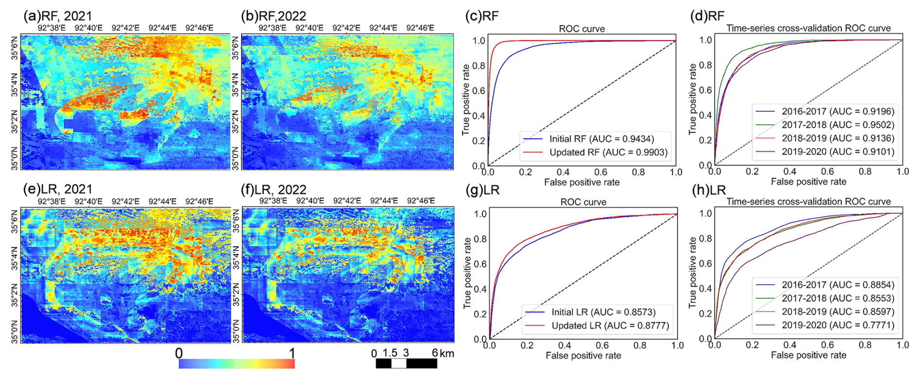
Figure 3 Performance evaluation and spatial predictions of the base probability models in the Beiluhe Basin. (a, b, e, f) Spatial distribution maps of predicted RTS occurrence probability for the 2020–2021 (a, e) and 2021–2022 (b, f) periods for the Random Forest (RF) (a, b) and Logistic Regression (LR) (e, f) models, respectively. (c, g) Receiver Operating Characteristic (ROC) curves illustrating the performance improvement before (Initial) and after (Updated) hyperparameter optimization. (d, h) Results of the rolling time-window cross-validation.

Based on the hyperparameter-optimized models, occurrence probability maps were predicted for the Beiluhe Basin for the 2020–2021 and 2021–2022 periods (Fig. 3a, b, e and f). A visual analysis reveals significant similarities between the predictions of both the RF and LR models. In both years, the models agreed on the general spatial pattern, identifying the highest RTS occurrence probabilities in the central regions of the basin while assigning lower probabilities to the peripheral areas. This overall pattern is consistent with the known distribution of existing RTSs. Despite this broad agreement, the models produced distinct spatial textures. The RF model's output is characterized by discrete, scattered patches of high probability (Fig. 3a for 2021, Fig. 3b for 2022), whereas the LR model yields continuous, ribbon-like zones with more gradual transitions between high- and low-risk areas, revealing finer spatial details (Fig. 3e for 2021, Fig. 3f for 2022). The LR model consistently identified a larger proportion of high-probability pixels (probability > 0.9) than the RF model in both 2021 (2.67 % vs. 2.07 %) and 2022 (1.12 % vs. 0.22 %). These high-risk zones from the LR model demonstrate a higher degree of spatial consistency with the observed clusters of actual RTSs. Comparing the predictions between the two years reveals subtle inter-annual variations that reflect the models' sensitivity to the different climate inputs. For instance, in the LR model's predictions, the peak probabilities appear slightly less intense and widespread in the 2022 map (Fig. 3f) compared to the 2021 map (Fig. 3e).

3.3 Model calibration and spatiotemporal simulation

In Experiment 3, the integrated Logistic Regression Evolution Model (LR-EM) and Random Forest Evolution Model (RF-EM) were first calibrated using the observed 2020 RTS distribution in the Beiluhe Basin as the reference target, with optimized parametric values presented in Table 2. In this calibration step, both models achieved a strong fit to the data (Table 3). While both models demonstrated high overall spatial accuracy with κ coefficients and F₁ Scores exceeding 88 %, these global metrics are inevitably inflated by the massive class imbalance inherent to regional geohazard modeling, where the vast majority of the landscape remains stable. A more stringent and realistic evaluation metric is the FoM, which evaluates only correctly predicted changes and excludes stable areas. In this regard, the LR-EM exhibited a superior ability to capture new growth, achieving a FoM of 20.05 %, which surpassed the RF-EM's 17.36 %. In comparable land-use and land-cover change (LUCC) simulation studies, FoM values commonly range between approximately 2 % and 25 %, particularly for rare or spatially clustered change processes (Pontius et al., 2008). Within this context, the FoM values obtained by RTSEvo are highly competitive and indicate a highly effective capture of the underlying expansion mechanisms. Furthermore, the model demonstrates a substantial relative improvement compared to baseline probability-only simulations, with FoM increases exceeding 29 % when our dynamic allocation process-based rules are included. Both calibrated models also effectively reproduced the observed spatial clustering; the Moran's I of the simulated results for both the LR-EM (0.603) and RF-EM (0.599) closely matched the Moran's I of the actual 2020 RTS distribution (0.596).

Table 3 Performance metrics for the spatial calibration (2020) and independent validation (2021–2022) of the Logistic Regression Evolution Model (LR-EM) and Random Forest Evolution Model (RF-EM). All metrics were measured by comparing the simulated results against the observed RTS distribution in the primary Beiluhe Basin study area for each respective year.

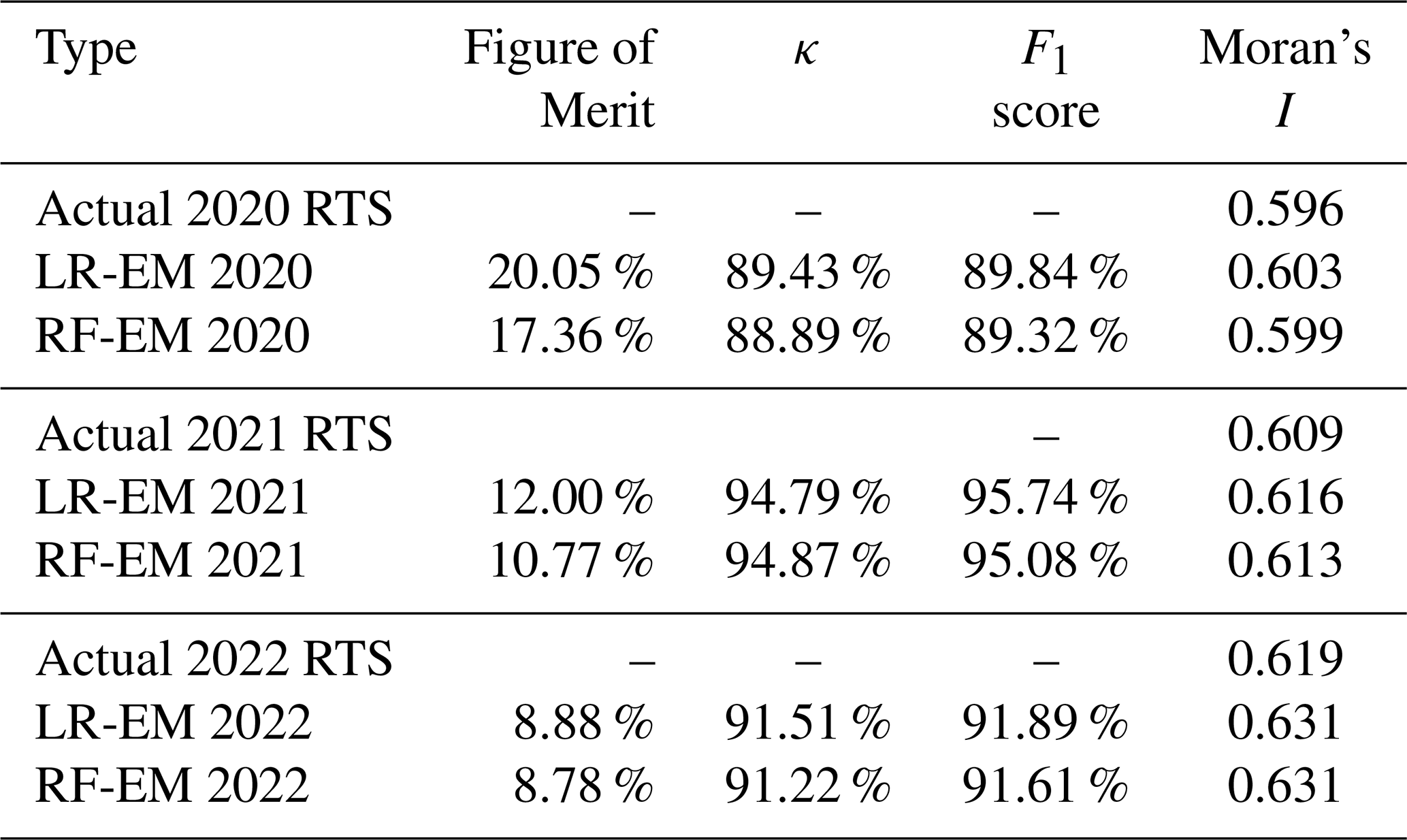
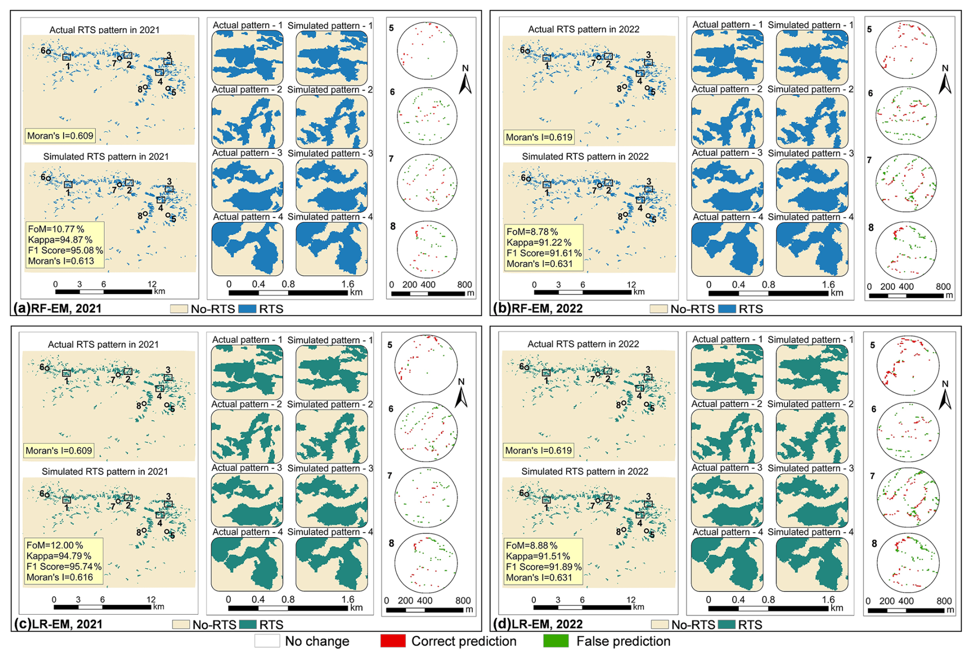
Figure 4 Comparison of simulated and observed RTS spatial distributions in the Beiluhe Basin for 2021–2022. The main maps show the overall simulated distributions and performance metrics for the (a) RF-EM in 2021, (b) RF-EM in 2022, (c) LR-EM in 2021, and (d) LR-EM in 2022. The rectangular inset panels (numbered 1–4) provide a detailed visual comparison between the observed (“Actual pattern”) and simulated slump morphologies for four representative sub-regions randomly selected from areas of intense RTS expansion. The circular insets (numbered 5–8) provide a pixel-level spatial evaluation of simulated versus observed RTS expansion. Note that the 2022 expansion simulations in the circle insets show the cumulative change from 2020 to 2022. Correct prediction (Red): Pixels that were correctly simulated as new RTS growth (Hits). False prediction (Green): Pixels representing either observed growth that the model missed (Misses) or areas incorrectly simulated as growth (False Alarms). No change (Blank/White): Areas that correctly remained non-RTS in both the simulation and reality.

Following calibration, the models with their optimized parameters were used for a predictive simulation of RTS evolution for the subsequent years, 2021 and 2022, which served as an independent validation. The LR-EM model consistently outperformed the RF-EM in both validation years in terms of absolute accuracy (Table 3). In 2021, the LR-EM achieved a FoM of 12.00 % compared to 10.77 % for the RF-EM. However, the accuracy of both models notably declined in 2022. Rather than a structural failure of the model, this drop is likely linked to a severe, anomalous summer heatwave occurred that year (Zhu et al., 2024), which introduced extreme non-linear thermal forcing that deviates from the baseline conditions used for calibration. This extreme climatic event highlighted differences in model robustness; while the RF-EM's performance declined less sharply, the LR-EM still maintained higher overall accuracy scores (FoM, κ, and F₁ Score) in both validation years. A spatial analysis of the simulation errors (Fig. 4) provides further insight. It reveals that while the models correctly identify the active margins of existing slumps as the primary zones for new growth, they struggle to pinpoint the precise, pixel-by-pixel location of that expansion. Most errors, both observed growth that the model missed (Misses) and areas incorrectly simulated as growth (False Alarms), are concentrated along these active boundaries. Visually, the LR-EM tended to produce larger, more contiguous clusters of correctly predicted pixels (Hits), which is consistent with its higher FoM score (Fig. 4c and d).

Despite variations in pixel-level accuracy, both models demonstrated excellent performance in reproducing the overall spatial patterns of RTS development. The average relative error of the Moran's I index was controlled within 1.5 % for both models, validating the effectiveness of the spatial allocation rules in capturing the characteristic regional clustering of RTSs. Furthermore, a qualitative comparison of slump morphology in the validation areas (Fig. 4) shows that the simulations successfully captured the general shape, size, and orientation of observed RTS expansion. The simulated slump boundaries, however, were generally smoother and less intricate than their real-world counterparts, indicating that while the model excels at capturing the macro-scale physical process, it tends to simplify complex, fine-scale topographic boundary details.

3.4 Model transferability and cross-regional generalizability

Evaluating the model's cross-regional generalizability revealed the physical limitations of direct parameter transfer across heterogeneous permafrost environments (Experiment 4). Baseline parameters derived from the highly concentrated RTS samples in the Beiluhe Basin proved strictly optimized for that region's specific climate forcing. When testing the Holt's linear trend model in the Haiding Nuo'er Subregion, an independent test area, the module achieved strong areal demand forecasting performance (R²=0.913, MAPE = 13.75 %). However, this regional forecast required a higher smoothing coefficient (α=0.8401) and a lower trend smoothing coefficient (${\mathit{\beta }}^{*}=\mathrm{0.4330}$) relative to the Beiluhe Basin. These parameter differences indicate that the temporal dynamics and climatic responsiveness of RTS expansion differ meaningfully between the two regions.

During the spatial allocation phase, the base occurrence probability maps generated by the LR module for the Haiding Nuo'er Subregion (Fig. S3) revealed that high probability zones are predominantly distributed in elongated, ribbon-like patterns adjacent to existing RTS features. Applying the direct transfer of Beiluhe Basin spatial allocation parameters to the Haiding Nuo'er Subregion yielded baseline FoM values of 15.81 %, 5.27 %, and 6.10 % for 2020, 2021, and 2022, respectively. Conversely, locally recalibrating the parameters based on the 2020 RTS distribution of the secondary site produced notable performance improvements, increasing the FoM to 18.15 % in 2020 and 6.25 % in 2021, although a modest decrease to 4.29 % was observed in 2022 (Fig. 5).

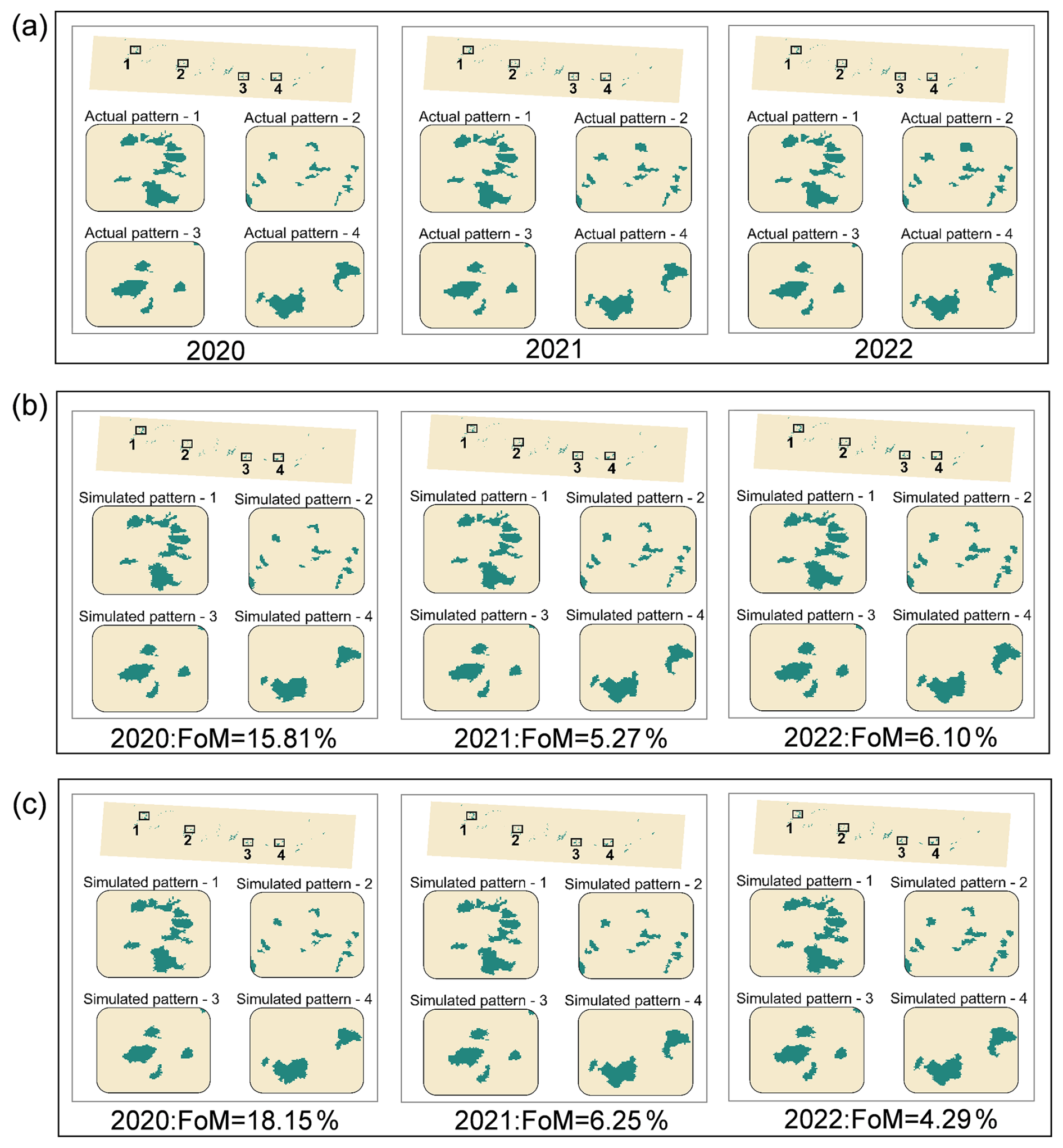
Figure 5 Comparison of simulated and observed RTS spatial distributions in the independent transferability test region (Haiding Nuo'er Subregion) for the 2020–2022 period. (a) Observed RTS spatial distributions based on historical inventories. (b) Simulated RTS spatial distributions using parameters directly transferred from the primary Beiluhe Basin without modification. (c) Simulated RTS spatial distributions using parameters locally recalibrated specifically for the Haiding Nuo'er Subregion.

These performance outcomes demonstrate that the RTSEvo architecture remains fully operational and capable of simulating RTS evolution when deployed in a different permafrost region. At the same time, the consistent accuracy gains achieved through local recalibration prove that spatial allocation parameters exhibit limited cross-regional generalizability. This finding highlights a reality of permafrost geomorphology: local topography, soil composition, and thermal forcing heavily modulate RTS expansion, necessitating region-specific optimization to achieve maximum predictive accuracy.

4 Discussion

4.1 Advancing from static susceptibility to dynamic evolution

While traditional RTS research has heavily relied on static susceptibility mapping, which successfully identifies high-risk spatial zones, these approaches inherently fail to capture the temporal evolution and physical propagation of these dynamic features. Our framework represents a paradigm shift in permafrost geohazard modeling by introducing a dynamic spatial allocation module constrained by a macro-scale area demand. This approach offers three key scientific advantages: (1) it ensures that simulated local spatial patterns are strictly anchored to observed regional expansion trends; (2) its rigorous calibration yields higher predictive accuracy in reproducing the realistic morphologic extent and clustering of RTS development; and (3) it provides a true predictive capability that is essential for forecasting RTS response under future climate scenarios.

From a scientific and practical standpoint, this predictive power is invaluable for engineering and environmental planning. It provides a more robust tool for assessing short- and long-term risks to critical infrastructure in permafrost regions and offers a quantitative method for understanding the cascading impacts of permafrost degradation, such as the mobilization of previously frozen carbon. However, this dynamic approach also introduces modeling challenges. A key issue is the potential for error propagation, where small inaccuracies in early simulation steps can accumulate over time, leading to deviations in long-term predictions. Furthermore, the base probability models showed some sensitivity to non-stationary environmental conditions. This was particularly evident in 2022, when a severe summer heatwave altered permafrost stability and led to a decline in simulation accuracy. This highlights a vulnerability of pure data-driven models when extrapolating to extreme, anomalous climatic events that are not well-represented in their historical training data.

While the RTSEvo model adopts its core top-down demand and bottom-up allocation structure from established LUCC modeling framework, it is technically specialized for geohazard simulation in two fundamental ways. First, and most critically, unlike many LUCC models where transition rules are set empirically based on expert knowledge, RTSEvo integrates mechanistic, process-based rules by embedding a direct physical understanding of terrain failure into the allocation rules. Second, the model implements a systematic optimization routine driven by maximizing FoM, ensuring the algorithm explicitly learns the behavior of new slump growth rather than just static background features.

4.2 The critical role of process-based rules

A central innovation of RTSEvo is the explicit integration of physical geomorphic processes, particularly the retrogressive erosion factor, into a data-driven framework. Our comparative experiments in the Beiluhe Basin definitively quantify the value of this approach. When comparing baseline models (using only statistical occurrence probability) against the full evolution models for the 2020 calibration year, the results were obvious: the FoM for the LR-based model increased from 6.67 % (baseline) to 20.05 % (full model), while the RF-based model's FoM jumped from a mere 0.42 % to 17.36 %. This massive discrepancy demonstrates that spatial allocation rules are absolutely essential for accurately capturing RTS evolution.

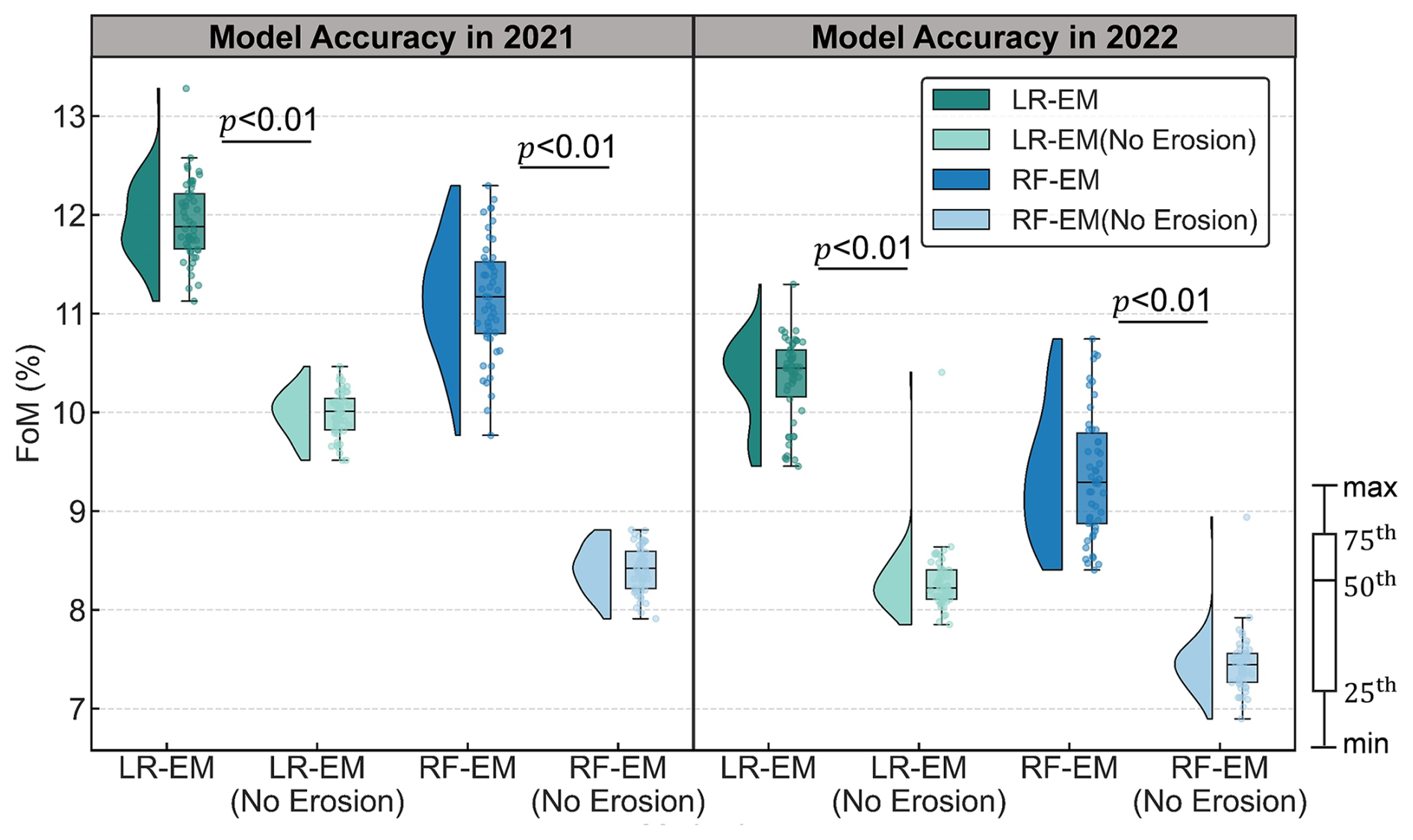
Figure 6 The impact of the retrogressive erosion factor on simulation accuracy for 2021 and 2022 in the Beiluhe Basin. “No Erosion” denotes the performance of the models when the physical retrogressive erosion allocation rule is deactivated.

To specifically isolate the contribution of the retrogressive erosion factor, we conducted a sensitivity analysis comparing the full evolution models with and without this single factor across 50 randomized trials (Fig. 6). The results confirm that excluding this physical rule led to a statistically significant (p<0.01) reduction in simulation accuracy. In the 2021 validation, its inclusion improved the FoM from 9.99 % to 11.94 % for the LR-EM, and from 8.41 % to 11.15 % for the RF-EM. The stabilizing power of this physical constraint was even more pronounced during the anomalous 2022 heatwave, where its inclusion drove massive relative FoM improvements of 29.3 % for the LR-EM and 22.3 % for the RF-EM.

The theoretical importance of this factor stems from its ability to encode fundamental geomorphic feedbacks that are otherwise absent in purely statistical frameworks. In natural RTS evolution, headwall retreat is governed by thermally driven ice melt and subsequent slope failure, which cause a highly directional growth pattern. By introducing a directional weighting term aligned with upslope retreat, the model effectively reduces spatial randomness in cell transitions and enhances spatial autocorrelation that is strictly consistent with observed morphodynamics. The larger relative improvement observed in 2022 highlights a modeling reality. Because extreme thermal forcing diminished the predictive reliability of the purely statistical components during that specific year, the physical rule provided by the erosion factor acted as a critical anchor. It guided the simulation toward a physically plausible outcome even when the statistical relationships temporarily broke down.

To further understand the underlying environmental drivers of RTS initiation, a SHapley Additive exPlanations (SHAP) analysis was performed (Fig. A4). The results identified maximum summer temperature (mean SHAP value: 0.09) and ground ice content (0.087) as the two most influential factors, representing the key energy input and material basis for RTS development. Factors of moderate importance, such as land cover and geology, reflect the synergistic control of surface conditions. In contrast, precipitation parameters exhibited relatively weaker impacts. This temperature-dominance strongly aligns with the known mechanisms of permafrost degradation on the QTP, corroborating field observations that link RTS events to anomalously high thermal energy inputs (Lewkowicz and Way, 2019; Luo et al., 2022a).

4.3 Predictor resolution and the scale-mismatch challenge

A practical challenge in regional permafrost modeling is the scale mismatch between local geomorphological features and the coarse resolution of continuous satellite-derived environmental predictors. In the Beiluhe Basin, individual RTS features have a mean area of 2.61 ha, corresponding to an approximate diameter of 160 m. When predictors like MODIS NDVI (250 m) or reanalysis climate forcing are resampled to 10 m modeling grid, sub-pixel spatial heterogeneity is not explicitly represented. In traditional susceptibility mapping, this scale gap typically results in overly smooth, unrealistic hazard zones that fail to capture the sharp boundaries of actual terrain failure.

RTSEvo is designed to mitigate this scale gap through its two-stage modeling structure, which mathematically isolates the smoothing effect. In the first stage, the probability estimation module uses regional-scale predictors merely to identify permissive bioclimatic areas where RTS expansion is environmentally plausible. In the second stage, the constrained spatial allocation module determines how RTS expansion is actually expressed at high spatial resolution. This allocation process is controlled by neighborhood interactions and RTS expansion rules, allowing fine-scale spatial patterns to emerge even when the background predictors are spatially smooth.

To rigorously validate this structural merit, we focused our sensitivity testing on vegetation (NDVI). Vegetation is a critical modulator of ground thermal regimes and was confirmed as a meaningful predictor in our SHAP analysis (Fig. A4). We tested whether its coarse representation was bottlenecking our simulation. Upgrading the vegetation input from 250 m MODIS to a reconstructed 30 m Landsat 8 NDVI dataset for the 2021 independent simulation in the Beiluhe Basin yielded only marginal performance gains (<1.2 % FoM increase) (Figs. S4 and S5). This counterintuitive finding reveals that while finer-resolution vegetation data naturally enhances local contrast, vegetation density only indicates general environmental susceptibility. Because RTSEvo explicitly delegates physical constraints to the high-resolution spatial allocation module, it prevents the smoothing effect of coarse predictors from destabilizing the final simulation.

This finding carries significant operational implications for permafrost geohazard forecasting. High-resolution imagery (e.g., 30 m or finer) on the QTP frequently suffers from severe temporal limitations, including frequent cloud contamination and irregular acquisition intervals. Our results demonstrate that regional simulation efforts do not need to be bottlenecked by the absence of high-resolution datasets. By combining coarse but temporally consistent environmental data with strict, physically based allocation rules, researchers can generate highly realistic, fine-scale evolutionary projections.

4.4 Model transferability and regional permafrost heterogeneity

The parametric sensitivity observed during our cross-regional validation is not a structural limitation of the RTSEvo algorithm, but rather a direct reflection of the profound spatial heterogeneity inherent to permafrost landscapes. Because RTS expansion is fundamentally a phase-change driven geomorphic process, regional variations in subsurface thermal regimes, active layer thickness, and ground ice distribution physically alter how a slump propagates. Consequently, a parameter set highly optimized for the specific ice-rich, high-elevation environment of the Beiluhe Basin naturally misaligns with the distinct climatic and topographic boundary conditions of the Haiding Nuo'er Subregion. This confirms that while the universal physical rules encoded in the model (such as retrogressive erosion) remain valid across all environments, the statistical weights governing their local spatial expression cannot be universally transferred.

This physical reality exposes a critical vulnerability in the growing trend of applying monolithic, “one-size-fits-all” machine learning frameworks to pan-Tibetan or pan-Arctic permafrost simulations. Purely data-driven models trained on concentrated regional inventories risk severe spatial uncertainty and catastrophic predictive failure when extrapolated to novel environments because they conflate universal failure mechanisms with local environmental sensitivities. Our results prove that by mathematically separating universal physical mechanisms (the spatial allocation rules) from local environmental sensitivities (the occurrence probability weights), dynamic models developed a structural resistance to this deterioration and can be successfully ported across regions. However, to achieve reliable continental-scale projections, the permafrost modeling community still have to adopt a “regionalized” parameterization paradigm.

4.5 Limitations

Although the proposed evolution model demonstrates strong predictive capabilities for simulating RTS dynamics, several limitations remain. These primarily stem from inherent uncertainties in input data and necessary simplifying modeling assumptions.

A first source of uncertainty arises from the RTS inventory datasets used for model calibration and validation. While high-resolution imagery and field surveys minimize mapping errors, the delineation of slump boundaries remain subject to interpreter bias, seasonal visibility constraints, and the time gaps between observations .(Xia et al., 2024b; Nitze et al., 2025). These uncertainties inevitably propagate into the training samples and affect the model's reliability. The driving factor datasets also exhibit inherent limitations. While prepared at a high spatial resolution, they may not adequately capture highly localized or short-duration extreme events, such as acute heatwaves, intense precipitation, or seismic disturbances, that are known to play a key role in triggering or accelerating RTS activity (Yin et al., 2023; Chen et al., 2024; Nesterova et al., 2024; Luo et al., 2025). This omission likely contributed to the decline in model accuracy observed under the anomalous conditions of the 2022 extreme heatwave.

Beyond data-related issues, the modeling framework also embeds several theoretical assumptions that require careful consideration. The model assumes synchronicity between RTS mapping and environmental drivers by using annual snapshots of both. In reality, RTS initiation and expansion is likely to exhibit a time-lagged geomorphic response to climate and geomorphic forcing (Dai et al., 2025), suggesting that an annual resolution may oversimplify complex thermal-mechanical delays. Furthermore, the framework assumes that once a pixel converts to an RTS, it irreversibly remains in that state. This assumption is physically justified over short- to medium-term simulations. Field observations and remote-sensing studies consistently indicate that the processes of RTS stabilization, revegetation, and surface recovery typically operate over multi-decadal timescales, often exceeding 20 years, and are strongly modulated by local climate, sediment availability, and hydrological conditions (Burn and Friele, 1989; Leibman et al., 2014; Nesterova et al., 2024; Krautblatter et al., 2024). However, for extended temporal horizons (e.g., >30–50 years), neglecting stabilization and recovery processes may lead to a systematic overestimation of active RTS extent. Future iterations of the model must incorporate multi-class state transitions to simulate the recovery state of the RTS.

Therefore, future improvements should focus on integrating multi-source uncertainty quantification, incorporating event-based drivers such as extreme climate anomalies and seismic activity, and relaxing the irreversibility assumption to account for possible slump stabilization processes. These enhancements will improve the evolution model's robustness and generalizability across diverse permafrost environments.

5 Conclusions

In this study, we developed and validated RTSEvo, a novel dynamic evolution model for retrogressive thaw slumps (RTS). The model framework integrates three core modules: a time-series forecast to establish regional RTS areal demand, machine learning algorithms to map base occurrence probability, and a physically constrained spatial allocation module that incorporates neighborhood effects, stochasticity, and a retrogressive erosion factor. Based on independent validation on the QTP, the results yield four key conclusions:

1. Applied and validated in the Beiluhe Basin, QTP for the 2021 and 2022 periods, the model successfully simulated dynamic RTS expansion. The Logistic Regression-based model (LR-EM) achieved a Figure of Merit (FoM) of 12.00 % and simulated Moran's I values closely matching those of the actual RTS distribution in the independent 2021 validation, demonstrating its effectiveness as a robust new tool for forecasting RTS evolution in space and time.

2. While both the Random Forest (RF-EM) and LR-EM evolution models performed well, the simpler architecture of the LR-EM demonstrated superior predictive accuracy and temporal stability in both calibration and validation years.

3. The integration of physical, process-based rules is an absolute computational necessity for accurately simulating RTS behavior. Specifically, encoding the retrogressive erosion factor significantly enhanced model performance, increasing the FoM by up to 29.3 % compared to purely statistical simulations without this process, particularly during periods of extreme climatic forcing.

4. Cross-regional validation confirmed the structural generalizability of the RTSEvo framework across heterogeneous permafrost environments. However, it also highlighted a reality of permafrost geomorphology that spatial allocation parameters must be locally recalibrated to account for distinct regional variations in ground-ice distribution and thermal forcing to achieve optimal predictive accuracy.

The primary contribution of this work is the successful development of a framework capable of moving beyond static susceptibility mapping to the dynamic, regional-scale simulation of RTS evolution. This dynamic modeling framework provides a critical scientific basis for designing RTS-related risk mitigation strategies for critical infrastructure and for accurately quantifying the cascading impacts of permafrost degradation in a warming climate.

Appendix A

Table A1 Summary of potential environmental driving factors used for RTS modeling. Soil particle content (sand, clay, and silt) is provided for six depth layers (0–5, 5–15, 15–30, 30–60, 60–100, and 100–200 cm). Note that permafrost type was excluded as a variable in this study, as its uniformity across the study area offered no predictive power.

^* As RTS map from August captures the cumulative result of the entire summer thaw season, predictor variables cover the same period of the September-to-August “growth” year to avoid temporal mismatch.

Table A2 Results of statistical homogeneity tests evaluating the consistency of predictor variables between the training and testing dataset. All p values exceed the 0.05 significance level, confirming no significant distributional differences between the data splits. Clay60–100 and silt30–60 refer to the clay and silt contents at depths of 60–100 and 30–60 cm, respectively. TDD denotes thawing degree days, calculated as the sum of mean daily temperatures above 0 °C.

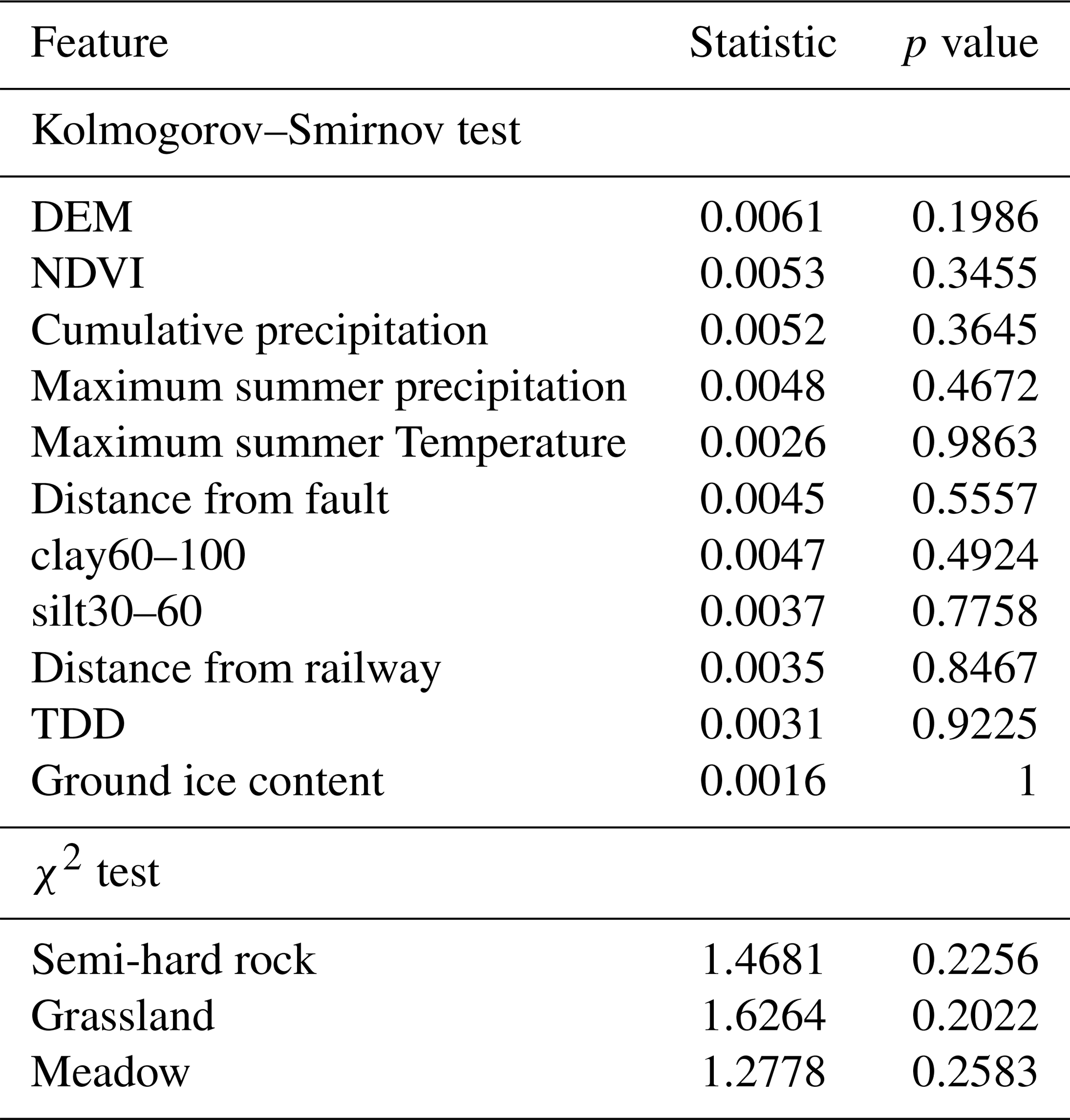
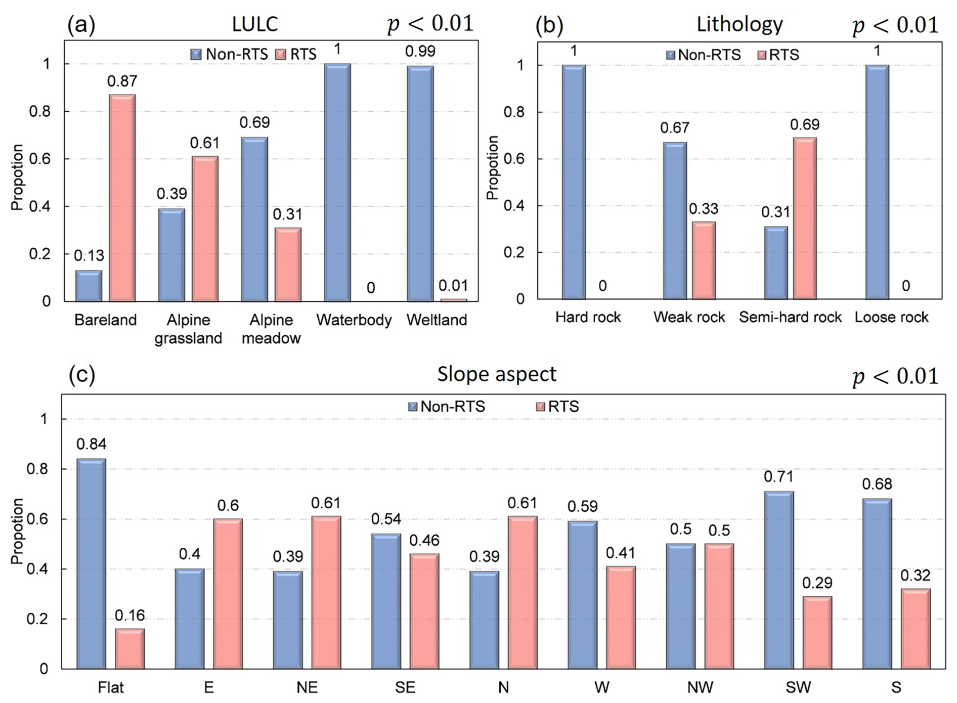
Figure A1 Frequency distribution of categorical predictor variables for RTS versus non-RTS locations. The bar charts compare the relative frequencies of categories for (a) land use/land cover, (b) lithology, and (c) slope aspect. χ² tests indicate a statistically significant difference (p<0.01) between the RTS and non-RTS groups for all variables shown.

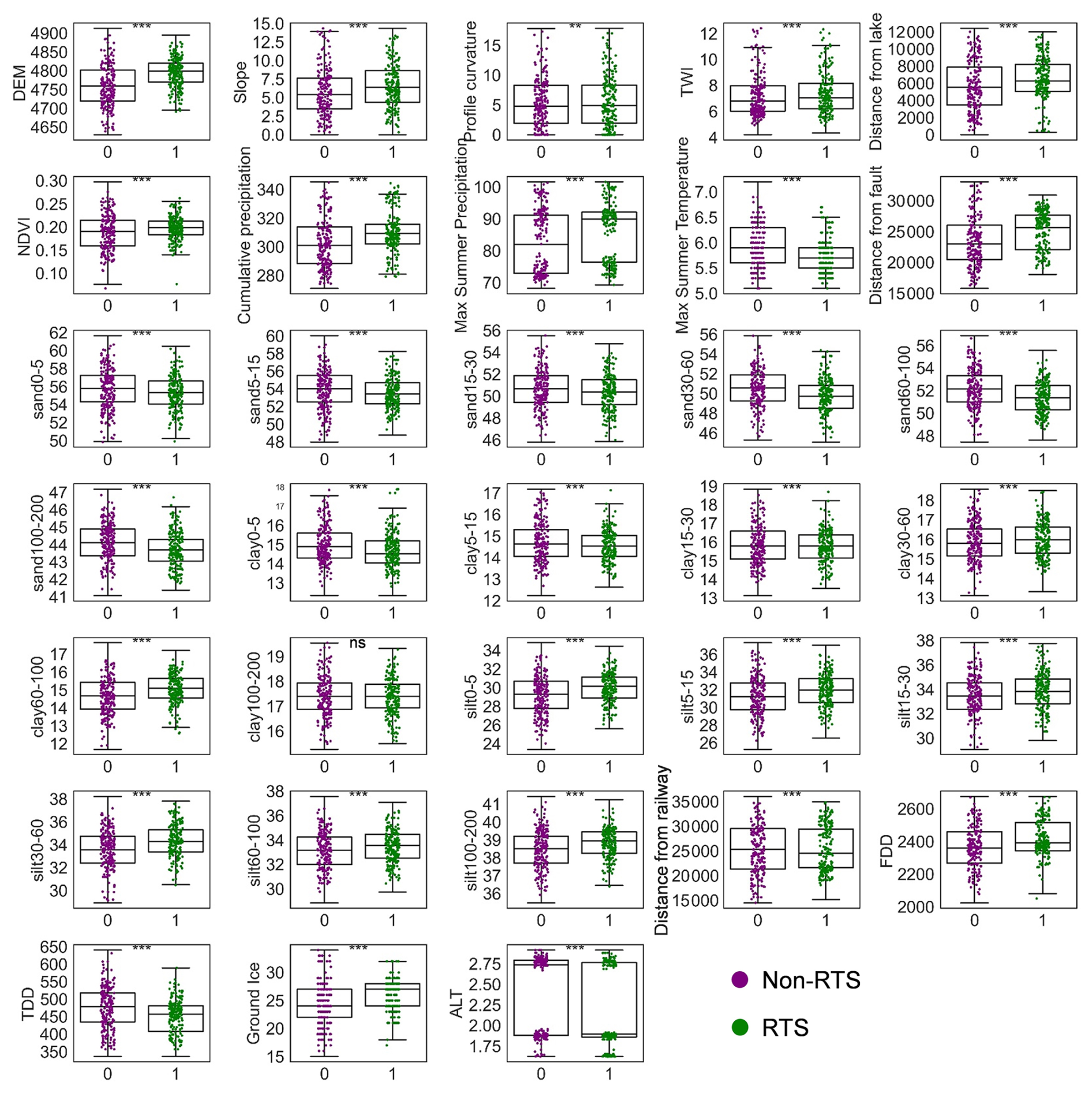
Figure A2 Distribution of numerical predictor variables for RTS versus non-RTS locations. The box-and-whisker plots compare the distributions between zones with RTS occurrence (RTS = 1) and stable, non-RTS zones (RTS = 0). Significance levels between the groups, determined by the Mann–Whitney U test, are indicated as follows: ns, not significant; ^* p<0.05; ${}^{**}$ p<0.01; ${}^{***}$ p<0.001.

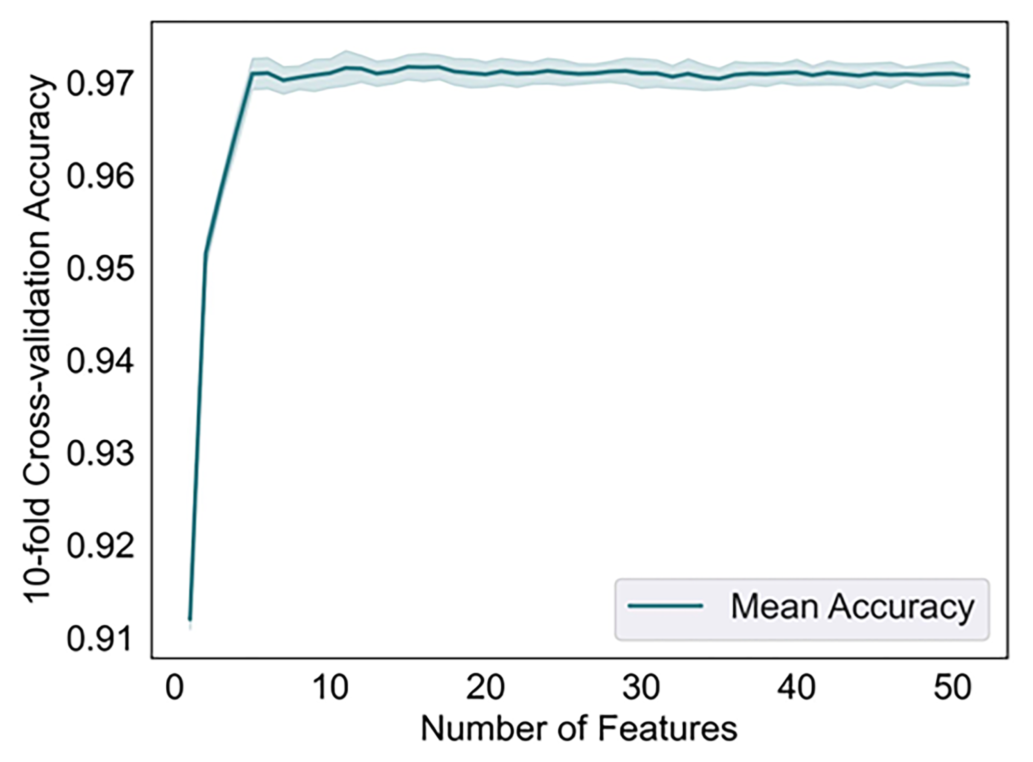
Figure A3 Feature selection curve from the Recursive Feature Elimination with Cross-Validation analysis. The curve plots the mean 10-fold cross-validation accuracy against the number of features included in the model, with the shaded envelope representing ±1 SD (standard deviation). Peak model accuracy (0.97) is achieved with an optimal subset of 14 features, which was used for the final model.

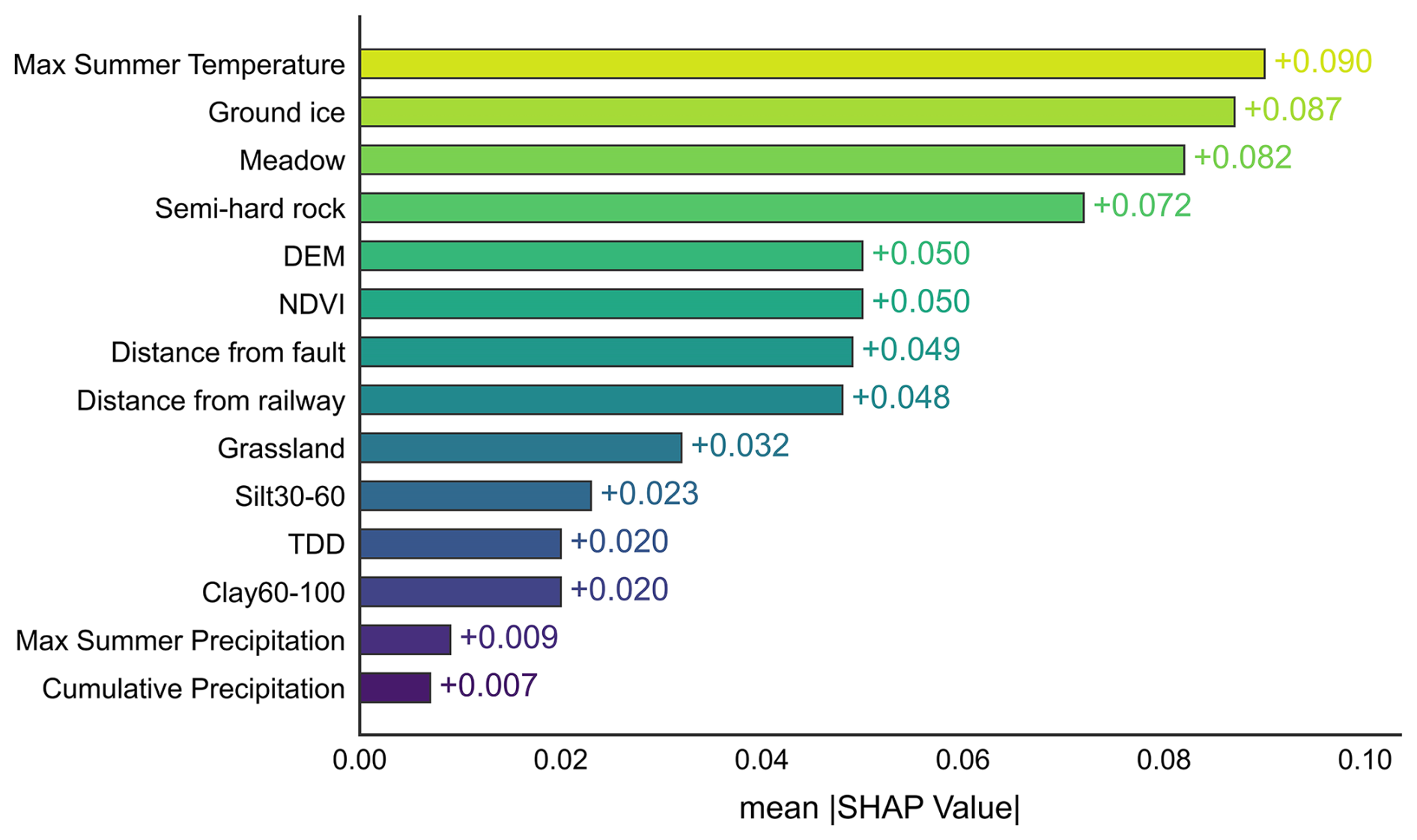
Figure A4 Global feature importance ranking based on mean absolute SHapley Additive exPlanations (SHAP) values.