MinSIA v1: a lightweight and efficient implementation of the shallow ice approximation

Simulations of ice flow have recently been boosted to an unprecedented numerical performance by machine learning techniques. This paper aims at keeping classical numerics competitive in this field. It introduces a new numerical scheme for the shallow ice approximation. Key features are a semi-implicit time-stepping scheme in combination with a dynamic smoothing of the nonlinearity in the slope-dependence of the flow velocity. As a first step, the software MinSIA presented here provides lightweight implementations of the new scheme in MATLAB and Python. MinSIA is designed for simulations on grids with several million nodes on standard desktop PCs and allows for spatial resolutions of 25 m or even finer. The numerical scheme performs particularly well for heavily glaciated topographies with moderately inclined ice surfaces. In turn, the advantage of the scheme decreases slightly for alpine topographies with steep walls during phases of moderate glaciation. The main limitation, however, arises from the simplified physics behind the shallow ice approximation, which becomes particularly severe in narrow valleys and if sliding along the bed is strong.

1 Introduction

Numerical glacier and ice-sheet models have been widely used in the context of climate change (e.g., Goelzer et al., 2020; Seroussi et al., 2020), paleoglacial reconstruction (e.g., Cohen et al., 2018; Seguinot et al., 2018; Weber et al., 2021), and long-term landform evolution (e.g., Braun et al., 1999; Egholm et al., 2012). While models of ice dynamics typically include a multitude of processes beyond the flow of ice (e.g., meltwater flow and heat transport), the latter is typically by far the computationally most expensive part.

Three-dimensional simulations of the Stokes equations with a free surface (as implemented, e.g., in the model Elmer/Ice) and the shallow ice approximation (SIA) are end-members in the hierarchy of ice-flow models. In its simplest form, the SIA reduces the problem to a single partial differential equation for the elevation of the ice surface by assuming hydrostatic pressure and neglecting all stresses arising from horizontal shearing. Mathematically, the SIA requires that the ice layer is thin compared to the horizontal length scale defined by the topography. In particular for alpine glaciers, this condition is typically not met. In order to overcome this limitation, several depth-integrated approaches that account for horizontal stress components were developed, such as the second-order approximation iSOSIA proposed by Egholm et al. (2011) and the Parallel Ice Sheet Model (PISM), which includes the shallow shelf approximation (Bueler and Brown, 2009).

Several benchmark experiments were performed in order to compare depth-averaged models to solutions of the full Stokes equations based on synthetic examples (e.g., Hindmarsh, 2004; Le Meur et al., 2004; Pattyn et al., 2008) or real-world scenarios (e.g., Seddik et al., 2017). These experiments confirmed the relevance of the theoretical limitations of the SIA concerning the topography and also pointed out its limited applicability to scenarios with fast sliding along the bed.

The numerical expense of all these models depends strongly on spatial resolution. Seguinot et al. (2018) achieved a spatial resolution of 1 km in a simulation covering the entire Alps (900×600 km) over a time span of 120 000 years with PISM. However, these simulations required high-performance computing facilities and a resolution of 1 km is by far not perfect for a complex topography with many valleys of various sizes. Cohen et al. (2018) achieved a spatial resolution of about 500 m in 3-D full Stokes simulations of the Rhine glacier with Elmer/Ice. Although the domain was smaller and the simulated time span was much shorter then in the study of Seguinot et al. (2018), these numbers tentatively suggest that the numerical advantage of depth-averaged models over full Stokes simulations is not as huge as it might be expected.

The limited computational performance of depth-integrated models arises from a combination of assuming hydrostatic pressure and the explicit time-stepping scheme implemented in almost all contemporary models (Bueler, 2023). The main problem is that local variations in the slope of the ice surface generate a horizontal pressure gradient in the ice column down to the bed and thus affect the velocity of the entire ice column. As a consequence, all depth-integrated models, including the SIA in its simplest form, are susceptible to short-wavelength oscillations in surface elevation. Explicit schemes can only avoid the resulting instability by small time increments, which decrease quadratically with decreasing grid spacing.

The limited progress concerning the numerical efficiency has motivated the development of alternative approaches. In the context of large-scale landform evolution, Deal and Prasicek (2021) and Hergarten (2021) independently developed an approach to simulate erosion of valley glaciers without simulating the flow of ice explicitly. Implemented in the landform evolution model OpenLEM, it allows for simulations with spatial resolutions of less than 100 m over millions of years, and a benchmarking with the iSOSIA model yielded promising results (Liebl et al., 2023). However, this approach circumvents the numerical issues of simulating the flow of ice for a specific application, but does not solve them.

The most remarkable alternative approach is based on deep learning. The Instructed Glacier Model (IGM) (Jouvet et al., 2021) is an ice flow emulator that uses a Convolutional Neural Network trained by a two- or three-dimensional fluid-dynamical model. It achieves a speedup of up to three orders of magnitude compared to the original models. Recently, a version has been developed that even does not require a numerical model for training, but integrates a Convolutional Neural Network directly in the numerical solver (Jouvet and Cordonnier, 2023).

The purpose of this paper is to challenge the hypothesis that the potential for further improvements in computational efficiency with classical numerical methods is limited (Jouvet et al., 2021). Despite the deficiencies of the SIA, this study only considers the SIA without extensions by horizontal stress components. The reason for this restriction is that the SIA can be formulated as a single partial differential equation, which makes the development of efficient numerical schemes much easier than for systems of differential equations. In this sense, the development proposed here is only a starting point with the perspective that parts of it can be transferred to models with a more elaborate stress balance in the future.

The approach presented in the following combines a semi-implicit time-stepping scheme as already implemented in a few models (Bueler, 2016; Wirbel et al., 2018) with a novel dynamic stabilization against small-wavelength oscillations. Implementations in MATLAB and Python are available. Since the MATLAB implementation was developed prior to the Python implementation, the numerical tests presented in this paper were performed with the MATLAB version. Further details are given in Sect. 7.

2 Scope and governing equations

MinSIA simulates the flow of ice on a given topography b(x,y) in a two-dimensional approximation in Cartesian coordinates. The vertical ice thickness $h(x,y,t)$ is the considered variable. The rate of change in ice thickness is defined by the volumetric balance equation

$$\begin{array}{}\text{(1)}& {\displaystyle \frac{\partial h}{\partial t}}=-\text{div}\mathit{q}+r\end{array}$$

where $\mathit{q}(x,y,t)$ is the two-dimensional flux density (volume per time and cross-section length), $r(x,y,t)$ the net rate of ice production and melting (thickness per time), and div the two-dimensional divergence operator.

Combining efficiency with maximum flexibility was the design goal of MinSIA. At the lowest level of complexity, simple predefined functions for q and r are offered, which do not require much additional programming for running the model. These functions can be combined with spatially and temporally variable parameter values for more complex applications. Finally, custom functions can be included, which also allow for coupling MinSIA with other models., e.g., for temperature.

The simple predefined model for the flux density is based on a decomposition into ice deformation and sliding along the bed,

$$\begin{array}{}\text{(2)}& \mathit{q}={\mathit{q}}_{\text{d}}+{\mathit{q}}_{\text{s}}.\end{array}$$

The contribution of deformation is described by the relation

$$\begin{array}{}\text{(3)}& {\mathit{q}}_{\text{d}}=-f_{\text{d}}{h}^{\mathrm{5}}\left(\cos \mathit{\beta }{)}^{\mathrm{8}}\right|\mathrm{\nabla }s{|}^{\mathrm{2}}\mathrm{\nabla }s,\end{array}$$

where

$$\begin{array}{}\text{(4)}& s(x,y,t)=b(x,y)+h(x,y,t)\end{array}$$

is the elevation of the ice surface and ∇s is its gradient. This relation is based on Glen's flow law, which assumes that the strain rate is proportional to τⁿ with n=3, where τ is the shear stress. For a detailed discussion of this relation and the value of the exponent n, readers are referred to Cuffey and Paterson (2010). The factor f_d mainly depends on temperature in reality.

The factor involving the cosine of the slope angle β of the ice surface with

$$\begin{array}{}\text{(5)}& {\cos }^{\mathrm{2}}\mathit{\beta }={\displaystyle \frac{\mathrm{1}}{\mathrm{1}+{\tan }^{\mathrm{2}}\mathit{\beta }}}={\displaystyle \frac{\mathrm{1}}{\mathrm{1}+|\mathrm{\nabla }s{|}^{\mathrm{2}}}}\end{array}$$

is a simple correction for steep slopes. It takes into account that the thickness perpendicular to the surface is lower than the vertical thickness and that driving forces by gravity are proportional to sin β instead of $\tan \mathit{\beta }=\left|\mathrm{\nabla }s\right|$. The correction is explained in the derivation of Eq. (3) in Appendix A. It compensates the apparent inadequacy of the SIA for thin layers at steep bedrock slopes reported by Le Meur et al. (2004, Fig. 5). However, it is less elaborate than the full version of the SIA for an inclined bed developed by Hutter (1983). While the full version allows for moderately different slopes of the bed and the ice surface, the simplified version considered here assumes that the bed is parallel to the ice surface. This simplified version is basically the same as the parallel sided slab elaborated by Greve and Blatter (2009, Sect. 7.2).

For sliding at the bed, the relation

$$\begin{array}{}\text{(6)}& {\mathit{q}}_{\text{s}}=-f_{\text{s}}{h}^{\mathrm{3}}{\left(\cos \mathit{\beta }\right)}^{\mathrm{5}}|\mathrm{\nabla }s{|}^{\mathrm{2}}\mathrm{\nabla }s,\end{array}$$

is used. It combines the ideas of Weertman (1957) and Bindschadler (1983) (see also Cuffey and Paterson, 2010, Chap. 7). As a strong simplification, Eq. (6) with a given value of the parameter f_s relies on the assumption that the water pressure at the bed is proportional to the normal stress, following some simple models of glacial erosion that do not consider meltwater hydraulics explicitly (Braun et al., 1999; Deal and Prasicek, 2021; Hergarten, 2021). A short derivation of Eq. (6) is given in Appendix B. It should, however, be emphasized that modeling sliding along the bed is still one of the major challenges in this field and that the applicability of the SIA is limited under fast sliding conditions (e.g., Hindmarsh, 2004; Pattyn et al., 2008; Seddik et al., 2017).

To make the model more flexible, the values of f_d and f_s may vary in space and time. This would, e.g., allow for taking into account their dependence on temperature in combination with a thermal model or taking into account water pressure explicitly.

The generic form of the flow law,

$$\begin{array}{}\text{(7)}& \mathit{q}=-D(h,|\mathrm{\nabla }s\left|\right)\mathrm{\nabla }s,\end{array}$$

with a user-defined function $D(h,|\mathrm{\nabla }s\left|\right)$, offers the highest degree of flexibility.

Taking into account that $\frac{\partial h}{\partial t}=\frac{\partial s}{\partial t}$, the considered differential equation then reads

$$\begin{array}{}\text{(8)}& {\displaystyle \frac{\partial s}{\partial t}}=\text{div}\left(D(h,|\mathrm{\nabla }s\left|\right)\mathrm{\nabla }s\right)+r,\end{array}$$

where the specific version defined by Eqs. (3) and (6) assumes

$$\begin{array}{}\text{(9)}& D(h,|\mathrm{\nabla }s\left|\right)=\left(f_{\text{d}}{h}^{\mathrm{5}}(\cos \mathit{\beta }{)}^{\mathrm{8}}+f_{\text{s}}{h}^{\mathrm{3}}{\left(\cos \mathit{\beta }\right)}^{\mathrm{5}}\right)|\mathrm{\nabla }s{|}^{\mathrm{2}}.\end{array}$$

The property D is denoted diffusivity in the following, although the diffusion equation formally only allows a dependence of the diffusivity on s (and thus on h), but not on ∇s.

Different approaches are also included for the net rate of ice production and melting, $r(x,y,t)$. The simplest model is piecewise linear with an equilibrium line altitude (ELA) z_e and a maximum rate r_max,

$$\begin{array}{}\text{(10)}& r\left(z\right)=\left\{\begin{array}{ccc}min\left(g_{+}\left(z-z_{\text{e}}\right),r_{max}\right)& \text{for}& z\ge z_{\text{e}}\\ g_{-}\left(z-z_{\text{e}}\right)& \text{for}& z<z_{\text{e}}\end{array}\right.\end{array}$$

applied to the ice surface ($z=s(x,y,t)$), where g₊ is the accumulation gradient (net rate of ice production per meter above the ELA) and g₋ is the ablation gradient (net rate of melting per meter below the ELA). A typical application would be a time-dependent ELA while keeping the other parameters constant. However, MinSIA allows for a variation of all parameter values in space and time as well as for replacing Eq. (10) by a custom function. Alternatively, $r(x,y,t)$ can also be defined directly for each cell of the grid at each time.

3 Numerical scheme and implementation

3.1 Semi-implicit time stepping

MinSIA employs a semi-implicit time-stepping scheme. This scheme combines an explicit discretization of the diffusivity with an implicit discretization for the diffusion process itself. The respective time-discrete version of Eq. (8) reads

$$\begin{array}{}\text{(11)}& {\displaystyle \frac{s(t+\mathit{\delta }t)-s\left(t\right)}{\mathit{\delta }t}}=\text{div}\left(D\left(t\right)\mathrm{\nabla }s(t+\mathit{\delta }t)\right)+r\left(t\right).\end{array}$$

This semi-implicit scheme already ensures stability for arbitrary time increments δt in the sense that perturbations remain bounded. Let us neglect ice production and melting (r=0) and consider the point with the highest ice surface at t+δt. Since the fluxes also refer to t+δt, this point must have lost ice towards all its neighbors. Therefore, the ice surface must have declined from t to t+δt at this point. In turn, the ice surface of the point with the lowest ice surface at t+δt must have risen. So the total variation in s decreases in each time step (unless a different behavior is enforced by production and melting or by the boundary conditions), regardless of δt. The resulting unconditional stability, however, neither ensures a reasonable accuracy nor a physically meaningful solution at large δt. Therefore, some extensions are necessary, which will be explained in the following sections.

3.2 Finite volumes with upstream diffusivity

MinSIA uses a finite-volume discretization of the domain with square cells. Since the finite-volume approach is based on the flux densities across the boundaries between adjacent cells, it requires the diffusivity $D(h,|\mathrm{\nabla }s\left|\right)$ at the cell boundaries. MinSIA uses an upstream scheme here, which means that the diffusivity of the node with the higher ice surface is adopted for the respective cell boundary.

The upstream scheme helps to maintain the volumetric balance. While the finite-volume scheme itself preserves the ice volume exactly, the semi-implicit scheme does not see the obvious condition h≥0 (equivalent to s≥b) since D is fixed during the time step. Therefore, negative values of h may occur, which have to be compensated afterwards. Setting negative values to zero causes a systematic increase in total volume. This problem predominantly occurs at the contact of valley glaciers with ice-free slopes. If D>0 at the contact of a glacier cell and a (higher) slope cell, the slope cell will deliver non-existing ice to the glacier. The upstream scheme ensures D=0 in this situation and thus avoids a permanent systematic increase in ice volume. However, the upstream scheme cannot avoid that cells flip from positive to negative values of h occasionally. This effect will be investigated numerically in Sect. 4.3.

3.3 Smoothing the slope in the diffusivity

While the semi-implicit scheme is unconditionally stable, the explicit treatment of $D(h,|\mathrm{\nabla }s\left|\right)$ still limits the accuracy. Regions with a high diffusivity tend to become rather flat in the next step, which then leads to a low diffusivity. It will be shown in Sect. 4.1 that these oscillations in the diffusivity result in staircase-shaped ice surfaces and oscillations in the ice surface. While these oscillations are limited by the decreasing total variation, reducing these oscillations to achieve a reasonable accuracy requires small time steps. For the high-resolution example considered in Sect. 4, a reasonable accuracy was achieved for $\mathit{\delta }t=\mathrm{1}/\mathrm{4096}$ years, while an explicit scheme was found to be stable for $\mathit{\delta }t=\mathrm{1}/\mathrm{32}\mathrm{768}$ years. So the semi-implicit only allows for an 8 times larger time increment in this example, which is not a great enhancement in view of the higher numerical effort per time step.

Therefore, a dynamic smoothing of the slope of the ice surface in the diffusivity $D(h,|\mathrm{\nabla }s\left|\right)$ is the central novel idea in MinSIA. The main challenge is to reduce the numerical artifacts arising from the explicit treatment of $\left|\mathrm{\nabla }s\right|$ in $D(h,|\mathrm{\nabla }s\left|\right)$ without introducing new artifacts. In particular, the typically small values of $\left|\mathrm{\nabla }s\right|$ at large glaciers should not be merged with high values of $\left|\mathrm{\nabla }s\right|$ at the adjacent slopes. This is achieved in MinSIA by assuming that the length scale of smoothing is proportional to the ice thickness and by using a thickness-weighted average instead of a simple arithmetic mean. In sum, these assumptions ensure that smoothing is weak at at low thickness, where smoothing is also typically not necessary, and that regions with high thickness are not affected strongly by adjacent regions with low thickness.

As a starting point, the slope of the ice surface is computed at each node (i,j) according to

$$\begin{array}{}\text{(12)}& {\left|\mathrm{\nabla }s\right|}_{i,j}=\sqrt{{\left|{\displaystyle \frac{\partial s}{\partial x}}\right|}_{i,j}^{\mathrm{2}}+{\left|{\displaystyle \frac{\partial s}{\partial y}}\right|}_{i,j}^{\mathrm{2}}}\end{array}$$

with the individual components approximated by

$$\begin{array}{}\text{(13)}& {\displaystyle }{\left|{\displaystyle \frac{\partial s}{\partial x}}\right|}_{i,j}={\displaystyle \frac{\mathrm{1}}{\mathrm{2}}}\left(\left|{\displaystyle \frac{s_{i,j+\mathrm{1}}-s_{i,j}}{\mathit{\delta }x}}\right|+\left|{\displaystyle \frac{s_{i,j}-s_{i,j-\mathrm{1}}}{\mathit{\delta }x}}\right|\right)\text{(14)}& {\displaystyle }{\left|{\displaystyle \frac{\partial s}{\partial y}}\right|}_{i,j}={\displaystyle \frac{\mathrm{1}}{\mathrm{2}}}\left(\left|{\displaystyle \frac{s_{i+\mathrm{1},j}-s_{i,j}}{\mathit{\delta }y}}\right|+\left|{\displaystyle \frac{s_{i,j}-s_{i-\mathrm{1},j}}{\mathit{\delta }y}}\right|\right)\end{array}$$

and δx=δy. In contrast to the conventional central difference quotient, the absolute values are taken individually for the left-hand and right-hand parts. While this modification has no effect for smooth inclined ice surfaces, it avoids the formation of unrealistic spikes in the ice surface at local maxima during the simulation.

Smoothing is implemented by computing the thickness-weighted average of $\left|\mathrm{\nabla }s\right|$ over a square,

$$\begin{array}{}\text{(15)}& {\left|\mathrm{\nabla }s\right|}_{i,j}^{\text{smoothed}}={\displaystyle \frac{{\sum }_{k=i-m}^{i+m}{\sum }_{l=j-m}^{j+m}{h}_{k,l}{\left|\mathrm{\nabla }s\right|}_{k,l}}{{\sum }_{k=i-m}^{i+m}{\sum }_{l=j-m}^{j+m}{h}_{k,l}}}.\end{array}$$

The sum extends over a square of 2m+1 cells along each coordinate axis. To achieve a smoothing scale proportional to the thickness, a nondimensional smoothing factor f is introduced in such a way that averaging is performed over a length of 2fh along each axis (so fh in each direction). In the context of Eq. (15), this implies

$$\begin{array}{}\text{(16)}& \left(\mathrm{2}m+\mathrm{1}\right)\mathit{\delta }x=\mathrm{2}fh\end{array}$$

and thus

$$\begin{array}{}\text{(17)}& m=f{\displaystyle \frac{h}{\mathit{\delta }x}}-{\displaystyle \frac{\mathrm{1}}{\mathrm{2}}}.\end{array}$$

However, m will typically not be an integer number. Therefore, the weighted average is computed for the two integer numbers around m and linear interpolation between the results is used. So smoothing starts gently as soon as $h>\frac{\mathit{\delta }x}{\mathrm{2}f}$.

The weighted average can be implemented efficiently by computing the cumulative sums

$$\begin{array}{}\text{(18)}& G_{i,j}=\sum _{k=\mathrm{1}}^i\sum _{l=\mathrm{1}}^j{h}_{k,l}{\left|\mathrm{\nabla }s\right|}_{k,l}\end{array}$$

and

$$\begin{array}{}\text{(19)}& H_{i,j}=\sum _{k=\mathrm{1}}^i\sum _{l=\mathrm{1}}^j{h}_{k,l}\end{array}$$

at first. Then the weighted average (Eq. 15) is obtained as

$$\begin{array}{}\text{(20)}& \begin{array}{rl}& {\left|\mathrm{\nabla }s\right|}_{i,j}^{\text{smoothed}}=\\ & {\displaystyle \frac{G_{i+m,j+m}-G_{i+m,j-m-\mathrm{1}}+G_{i-m-\mathrm{1},j+m}-G_{i-m-\mathrm{1},j-m-\mathrm{1}}}{H_{i+m,j+m}-H_{i+m,j-m-\mathrm{1}}+H_{i-m-\mathrm{1},j+m}-H_{i-m-\mathrm{1},j-m-\mathrm{1}}}}\end{array}\end{array}$$

3.4 The linear solver

The linear equation system to be solved in each time step is positive definite and sparse. To improve efficiency for partly ice-covered surfaces, it is reduced to the relevant nodes (ice-covered nodes and their direct neighbors) in each step.

The preconditioned conjugate gradients (PCG) method is used for solving the linear equation system. An incomplete Cholesky factorization is used as a preconditioner, whereby the version that compensates dropped nondiagonal elements at the respective diagonal elements turned out to be particularly suitable. A direct solver is also implemented for testing.

4 Numerical tests

The present-day topography of the Southern Black Forest was used for the numerical tests. The considered domain consists of a 60×60 km square centered to the highest peak (Feldberg, 1493 m). The publicly available 1 m terrain model (Landesamt für Geoinformation und Landentwicklung, 2025) was downsampled to a grid spacing of $\mathit{\delta }x=\mathit{\delta }y=\mathrm{25}$ m, resulting in a grid of 2400×2400 cells. The spatial resolution was chosen to investigate the accuracy and the efficiency of the numerical scheme within in the framework of the SIA. To the author's knowledge, such a high spatial resolution cannot be achieved at a reasonable computational effort by any existing scheme for the SIA or for a more elaborate model of ice flow. In turn, the considered topography contains several steep valleys where the physical limitations of the SIA become relevant. This topic will be briefly addressed in Sect. 6, but is not the primary subject of this paper.

The values $f_{\text{d}}=\mathrm{5.34}\times {\mathrm{10}}^{-\mathrm{5}}$ ${\mathrm{m}}^{-\mathrm{3}}{\mathrm{yr}}^{-\mathrm{1}}$ and f_s=3.56 ${\mathrm{m}}^{-\mathrm{1}}{\mathrm{yr}}^{-\mathrm{1}}$ are assumed for the flow parameters, corresponding to the values used by Deal and Prasicek (2021). For the net rate of ice production, the simple ELA-based approach (Eq. 10) was used with an accumulation gradient of $g_{+}=\mathrm{0.002}$ yr⁻¹ and an ablation gradient of $g_{-}=\mathrm{0.003}$ yr⁻¹. These values are oriented on the rates assumed in the model comparison of Liebl et al. (2023). All simulations were run over a time span of 3000 years with a constant ELA at z_e=1000 m, starting from an ice-free surface. This setup does not address anything that ever happened, but was designed as a simple scenario with a transition from isolated valley glaciers towards a continuous ice cap, as illustrated in Fig. 1.

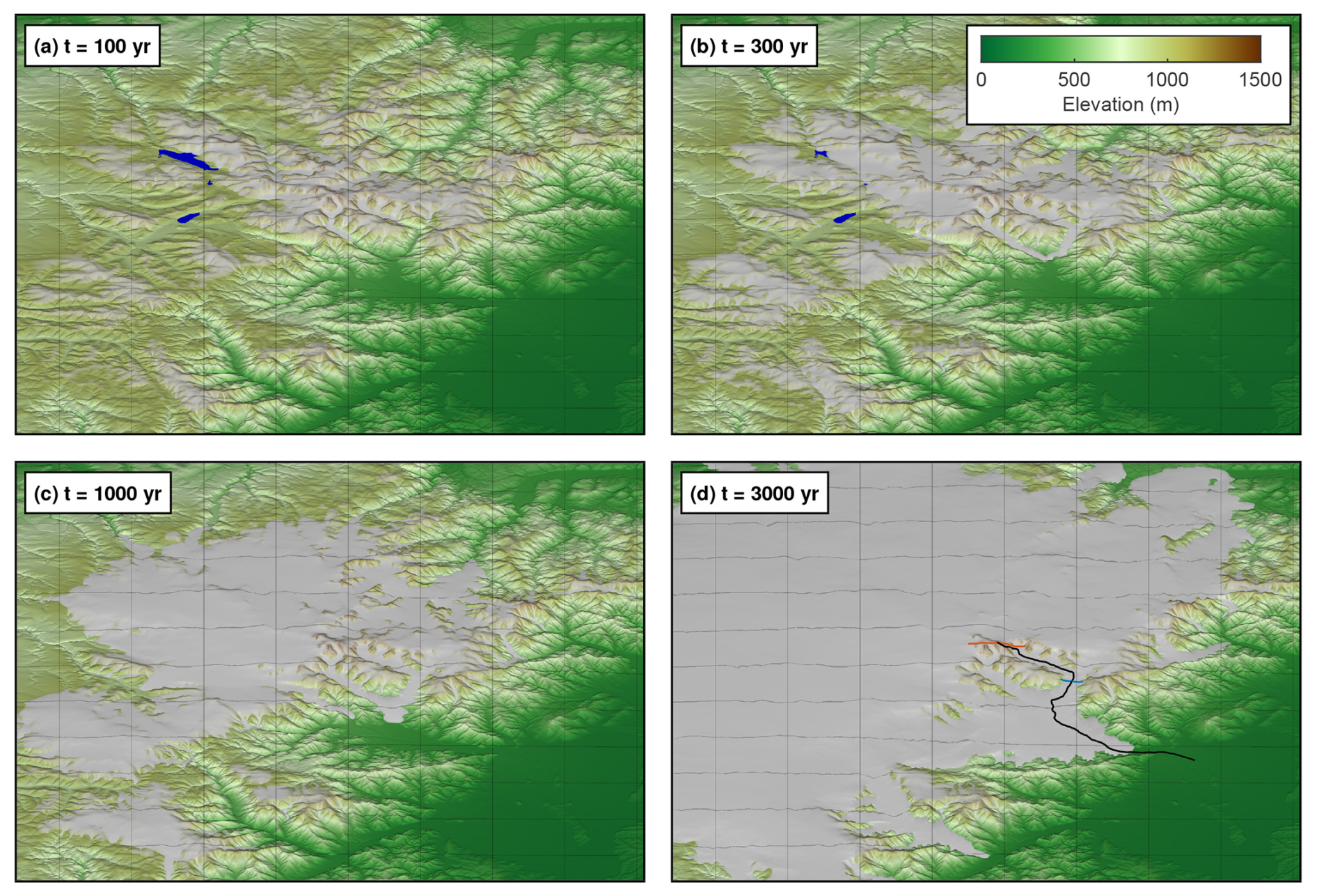
Figure 1 Snapshots from the reference scenario with a 5 km grid for illustrating the spatial scale. The black line in (d) refers to the longitudinal profile analyzed in Fig. 3, the blue line to the cross section shown in Fig. 11, and the red line to the profile through the highest peak shown in Fig. 12.

Time increment was $\mathit{\delta }t=\mathrm{1}/\mathrm{64}$ years and the smoothing factor was set to f=0.25 as a reference. As the maximum thickness achieved at the end was h=637 m, this choice corresponds to smoothing over squares of 13×13 cells (325 m; m=6 in Eq. 15) at maximum. While it would be desirable to use a simulation without smoothing as a reference scenario, the scenario considered here was originally chosen as a tradeoff between accuracy and numerical effort. The semi-implicit scheme without smoothing requires $\mathit{\delta }t=\mathrm{1}/\mathrm{4096}$ years and would have taken several months on a standard desktop PC. The error arising from the choice of the reference scenario will be discussed at the end of Sect. 4.1.

All simulations, except for the tests of the linear solver (Sect. 4.4), were performed either with the direct solver or with the PCG solver with a relative tolerance of 10⁻¹⁰. This value is small enough to ensure that the errors caused by the iterative PCG solver are negligible.

4.1 The effect of smoothing

As a first test, the accuracy of the solutions for different values of the smoothing factor f with respect to the reference solution (f=0.25, $\mathit{\delta }t=\mathrm{1}/\mathrm{64}$ years) is measured. For this purpose, the empirical cumulative distribution function (CDF) of the node-by-node deviation from the reference solution is computed, derived from all nodes covered by ice in either of the two compared scenarios.

The colored curves in Fig. 2 show an increase in deviation from the reference solution (f=0.25) with increasing f. Comparing the deviations at t=300 years (Fig. 2a) to those at t=3000 years (Fig. 2b) reveals an increase through time. This increase is, however, not only due to the accumulation of errors, but also goes along with the overall increase in ice thickness.

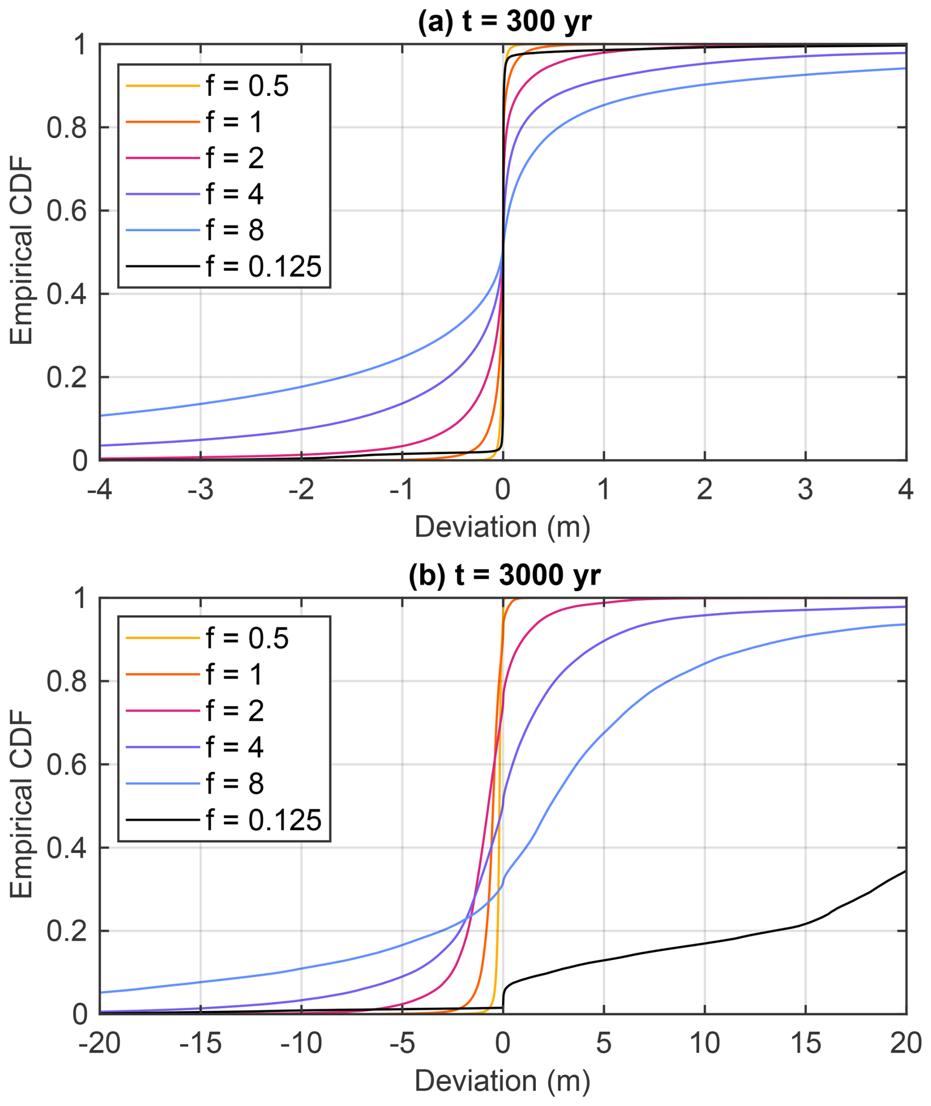
Figure 2 Deviation in ice thickness from the reference scenario (f=0.25). The empirical CDF was derived from all nodes covered by ice in either of the two compared scenarios.

To get a better feeling for the accuracy, Fig. 3 shows the longitudinal valley profile defined in Fig. 1d. The profile line follows the direction of the steepest descent of the bedrock topography. The profiles for f=0.5 and f=1 are visually indistinguishable from the reference profile, in agreement with the small deviations in Fig. 2. For f=1, 95 % of all deviations are in the range from −1.79 to 0.23 m at t=3000 years. While the deviation in the profile (Fig. 3) is still small for f=2, the ice surface is considerably too low for f≥4, in particular in the upper part of the glacier. Here the ice thickness is almost 100 m lower for f=8 than for f=0.25.

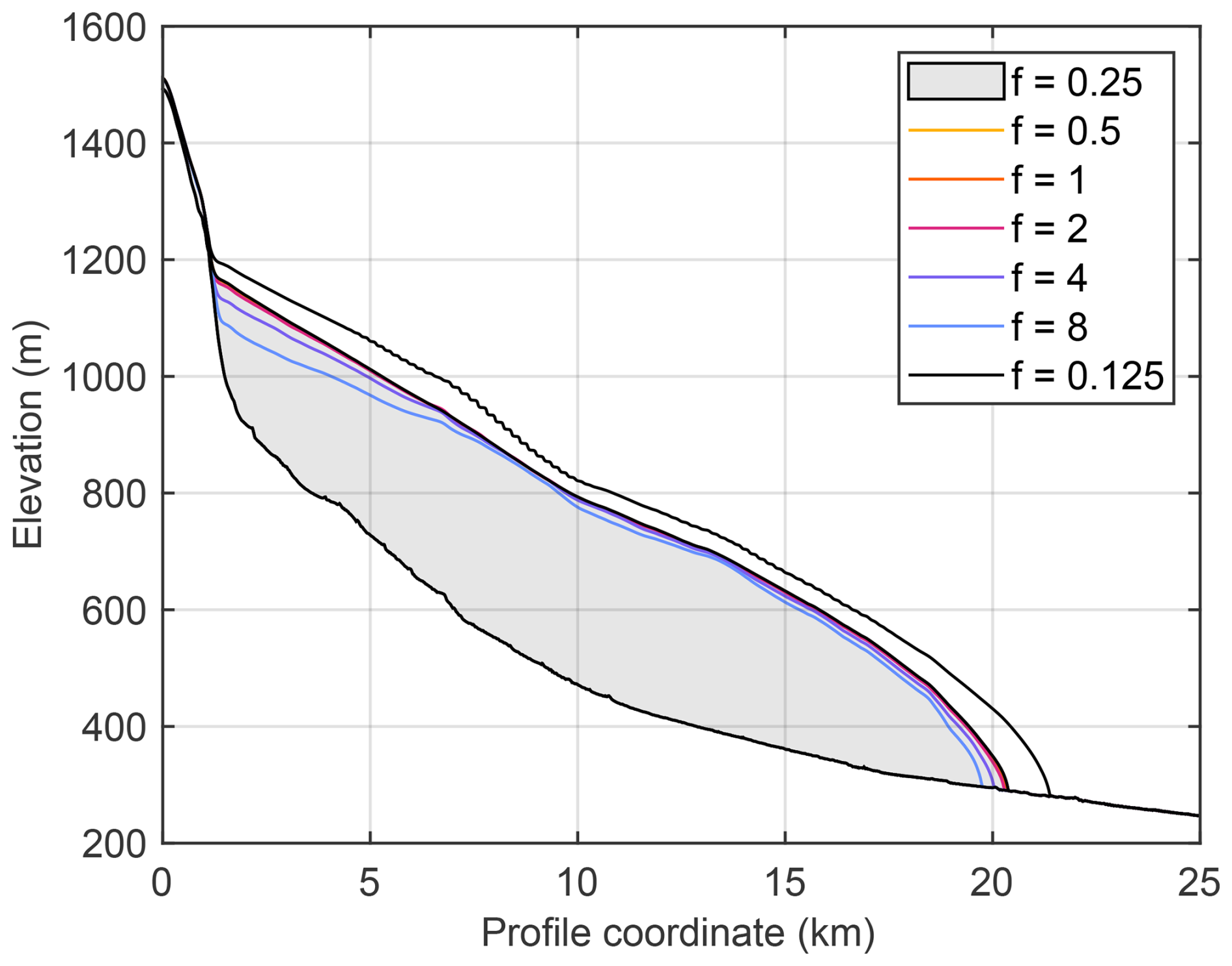
Figure 3 Longitudinal glacier profile along the line defined in Fig. 1d at t=3000 years for different values of f.

The behavior is completely different for f=0.125. The vast majority of all nodes has a very small deviation from the reference surface (f=0.25) at t=300 years (Fig. 2a). However, the distribution already shows quite long tails at both sides, reflecting a considerable deviation for a few percent of the nodes. The deviations become much larger at t=3000 years (Fig. 2b) with a strong trend towards large elevations. This trend is also visible in the glacier profile (Fig. 3), where the ice surface is systematically too high and the glacier is 1 km too long.

Figure 3 also reveals that the strong decrease in accuracy for f=0.125 goes along with staircase-shaped surface. One of the staircase-shaped sections is even considerably steeper than the reference surface. This means that the step-like shape has a negative effect on the ice flux, which must be compensated either by a greater thickness or a greater average slope. As mentioned above, a reference scenario without smoothing (f=0) would have required $\mathit{\delta }t=\mathrm{1}/\mathrm{4096}$ years, which was considered too expensive. To get an idea about the errors arising from the considered reference scenario, simulations over a shorter time span were conducted. While an analysis of convergence can be performed with an arbitrary initial condition theoretically, the end of the simulated time span is more representative here since smoothing has little effect in the early phase due to the low ice thickness.

The results shown in Fig. 4, obtained from a 100 year time span starting from the reference scenario at t=2900 years, suggest that the deviation from the solution with f=0 even decreases stronger than linearly with f. Comparing the root mean square deviations (0.0583 m for f=0.25 vs. f=0 and 0.158 m for f=0.5 vs. f=0) suggests that the error is proportional to f^1.43. The root mean square deviations of the full time span (0.262 m for f=0.5 vs. f=0.25, 0.778 m for f=1 vs. f=0.25, and 2.17 m for f=2 vs. f=0.25) yield the same dependence with an offset of 0.11 m, corresponding to the deviation between f=0.25 and the unknown solution for f=0. So the error of the reference scenario (f=0.25) is clearly smaller than the smallest deviations shown in Figs. 2 and 3 and is thus irrelevant for the considerations.

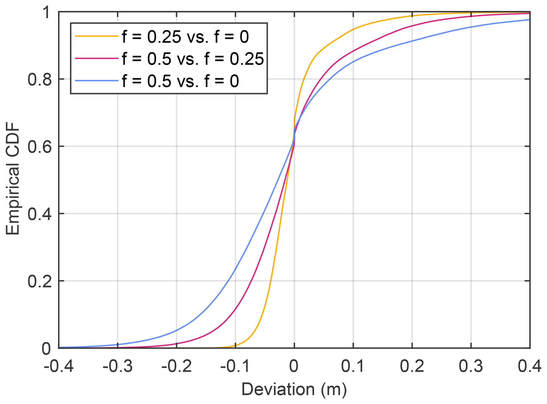
Figure 4 Deviation in ice thickness at t=3000 years obtained from simulations starting at t=2900 years. The empirical CDF was derived from all nodes covered by ice in either of the two compared scenarios.

4.2 The maximum time increment

Since even explicit schemes are stable for sufficiently small time increments, the occurrence of the staircase oscillation must be related to both the smoothing factor f and the time increment δt. It can be easily detected by tracking the elevation of the ice surface node by node without analyzing the topography of the ice surface. Let us define

$$\begin{array}{}\text{(21)}& \mathit{\delta }h\left(t\right)=\left\{\begin{array}{ccc}h(t+\mathit{\delta }t)-h\left(t\right)& \text{for}& h\left(t\right)<h(t-\mathit{\delta }t)\\ -\left(h(t+\mathit{\delta }t)-h\left(t\right)\right)& \text{for}& h\left(t\right)\ge h(t-\mathit{\delta }t)\end{array}\right..\end{array}$$

Positive values of δh describe points that decreased previously and increase now or increased previously and decrease now. So positive values of δh are a measure of the oscillation. MinSIA returns the maximum value of δh over all nodes in each time step.

Figure 5 shows the 95 % quantiles of the oscillation (still the maximum δh over all nodes in each step, but then the value that is not exceeded in 95 % of all time steps). Since not all changes from increasing to decreasing thickness or vice versa are necessarily numerical artifacts, the 95 % quantile is more useful than the maximum over all time steps. The exact choice of the quantile, however, is not important.

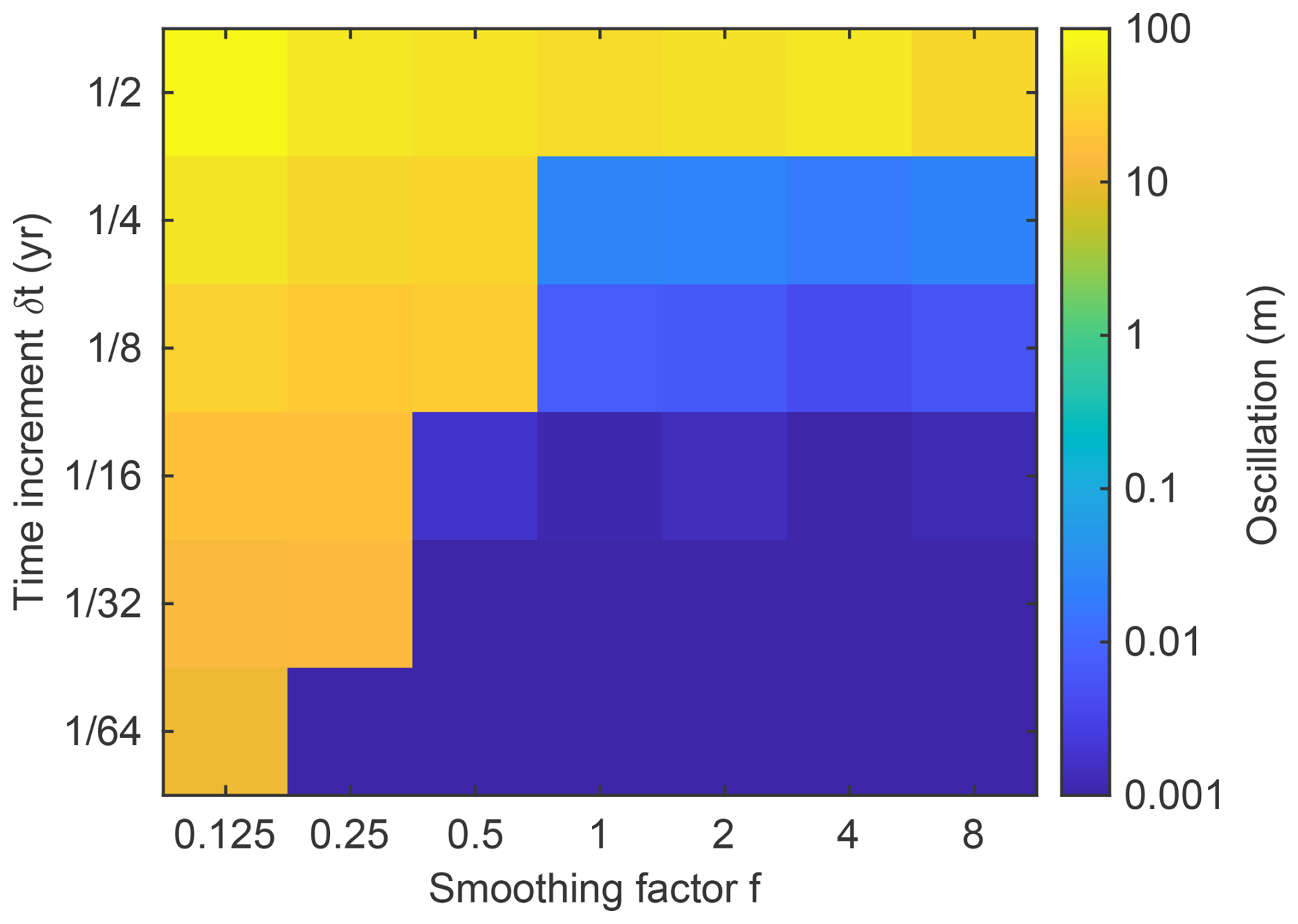
Figure 5 95 % quantiles of the maximum oscillation for different values of f and time increments δt.

The values of the 95 % oscillations show a clear distinction with only values above 10 m (yellow) and below 0.1 m (blue). So there is a clearly defined (at least within a factor of two) maximum time increment for each value of f. There seem to be two different regimes concerning the value of f. While the maximum δt increases strongly with increasing f for f≤1, it seems to remain constant for f>1.

At least for this example, this means that increasing the smoothing factor to values f>1 does not improve performance strongly. In combination with the good accuracy observed for f≤1 in Sect. 4.1, this finding suggests f=1 tentatively as a good tradeoff between accuracy and performance.

4.3 The volumetric balance

As discussed in Sect. 3.2, the upstream scheme cannot avoid an occasional occurrence of negative thickness values. These negative values have to be compensated (set to zero) to keep the ice surface consistent, which causes a systematic error in the volumetric balance.

Figure 6 shows the results of an analysis similar to that from Fig. 5, but for the total ice volume added throughout the simulation instead of the maximum oscillation. Effects of melting were removed from the considered volume. As an example, 2 m initial thickness, 1 m loss by melting, and 5 m loss by outflow would be only 3 m to be compensated.

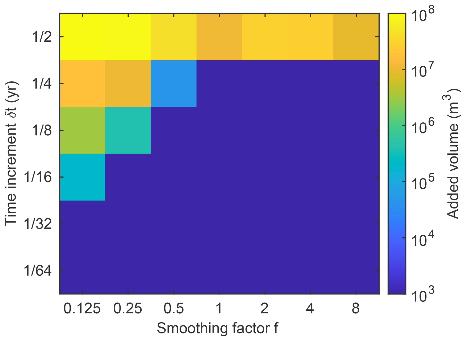
Figure 6 Total volume added throughout the simulation in order to keep the ice surface consistent (h≥0).

The result for the added volume looks qualitative similar to the result for the oscillation (Fig. 5) with only values below 1000 m³ (blue) and above 200 000 m³ (green to yellow). The transition takes place at higher δt than in Fig. 5 at least for f<1, which means that avoiding staircase oscillations defines a lower limit for δt than preserving the volumetric balance.

It should, however, be mentioned that even the highest added volume of about 1.4×10⁸ m³ is small in relation to the total volume of about 5×10¹¹ m³. To ensure that this result is not limited to advancing glaciers, two additional scenarios were considered. One of them assumes a sudden rise of the ELA to z_e=3000 m at t=3000 years, which lets all ice vanish within 100 years. The other scenario switches off ice production and melting at t=3000 years, so that the existing ice flows down toward the boundaries of the domain. The added volume per time is even lower than for advancing glaciers in both cases.

These results suggest that the systematic error in the volumetric balance is negligible compared to the immediate effect of the staircase oscillations on accuracy. So focus should be on limiting δt to avoid these oscillations.

4.4 The linear solver

The application of the iterative PCG solver is a tradeoff between accuracy and numerical effort. The version implemented in MinSIA uses the relative norm of the residuum (the default for the used MATLAB function) as a criterion for terminating the iteration, called tolerance in the following.

The colored lines in Fig. 7 show the error caused by the finite tolerance of the PCG solver for f=1 at t=3000 years, quantified by the root mean square deviation. Following the same concept as in Fig. 2, the deviation is derived from all nodes covered by ice in either of the two compared scenarios.

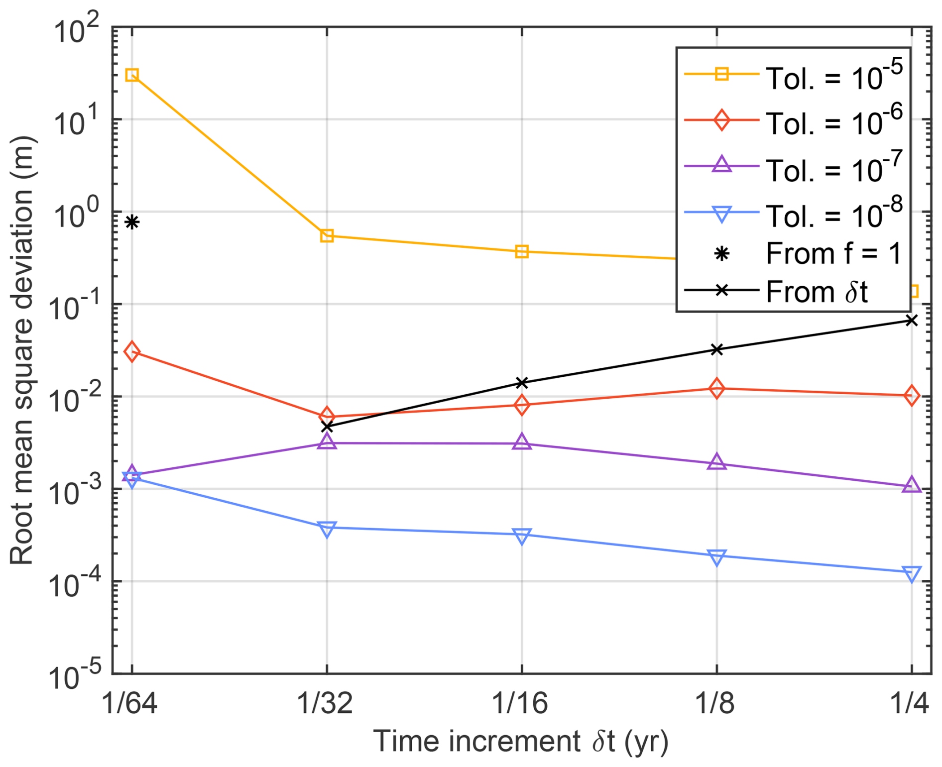
Figure 7 Root mean square deviations for f=1 at t=3000 years. Colored lines correspond to different tolerance levels of the PCG solver. Black lines and points correspond to the error arising from smoothing (f=1 vs. f=0.25) and from the finite time increment (actual δt vs. $\mathit{\delta }t=\mathrm{1}/\mathrm{64}$ years).

As long as the tolerance is not bigger than 10⁻⁶, the respective error is much smaller than the error arising from smoothing with f=1. Therefore, a tolerance of 10⁻⁶ is sufficient here. However, a decrease to 10⁻⁷ increases the numerical effort by less than 10 % here and thus provides an additional safety margin at reasonable cost. These results also hold for the coarser resolutions considered in the next section.

4.5 The spatial resolution

While the upstream scheme is necessary for maintaining the volumetric balance, it reduces the numerical accuracy. Upstream schemes achieve a linear convergence, which means that the numerical error due to the finite spatial resolution is theoretically proportional to δx in the limit δx→0. Schemes of higher order achieve a faster convergence.

The deviations in ice thickness between simulations with different resolutions are analyzed in Fig. 8. It is visually recognized that the respective deviations are roughly proportional to the change in δx at t=300 years (solid lines). This means that the theoretical linear convergence of the upstream scheme is confirmed here. At t=3000 years (dashed lines), however, the dependence of the deviation on δx is weaker than linear, indicating that linear convergence is practically not achieved here.

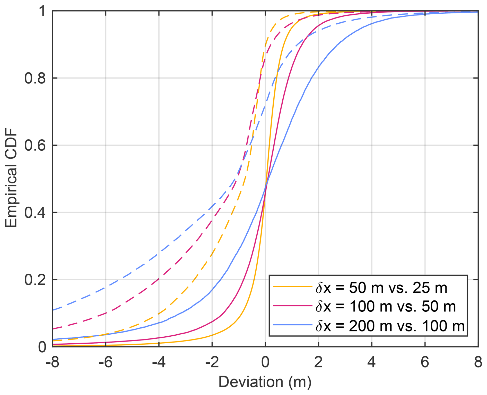
Figure 8 Deviation in ice thickness between simulations with different spatial resolutions. Solid lines refer to t=300 years and dashed lines to t=3000 years. The empirical CDF was derived from all nodes covered by ice in either of the two compared scenarios.

It is also recognized that the deviations arising from the finite resolution are considerably higher than those arising from smoothing at least for f≤1 (Fig. 2). From the mathematical point of view, this means that a high resolution, even with a grid spacing lower than the 25 m considered here, is useful. This argument is, however, only valid within the framework of the SIA and does not take into account the physical error due to neglecting horizontal stress components. This error may be much higher than the numerical error and will be discussed briefly in Sect. 6.

If there is a maximum stable time increment for a numerical scheme, it typically depends on the spatial resolution. Figure 9 shows the maximum time increment that avoids staircase oscillations for grids of different resolutions. A sudden increase in maximum oscillation at a certain time increment was observed for each set of simulations and a threshold of 1 m could be used consistently.

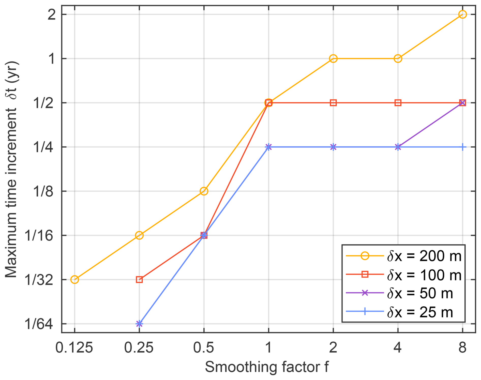
Figure 9 Maximum time increment that avoids staircase oscillations for different spatial resolutions.

Basically the same behavior was found for δx=25, 50, and 100 m. In particular, the benefit of values f>1 is small. Overall, a fourfold increase in δx increases the maximum δt by a factor of 2 at maximum. This decrease is small compared to the total number of nodes, which decreases by a factor of 16 here. So the immediate effect of the number of nodes on the computational effort is much stronger than the effect of changes in maximum δt. Increasing grid spacing to δx=200 m still has a minor effect on the maximum δt around f=1. However, the dependence on f becomes less clear. Instead of the distinct change in behavior at f=1, the maximum δt rather increases linearly with f.

The simulations over the entire time span with δt=0.25 years took 35 400 s for δx=25 m, 6740 s for δx=50 m, and 1290 s for δx=100 m on an Intel Core i5-7600 CPU (3.50 GHz) from 2018 with the MATLAB implementation. Since no dedicated parallel computing options were used, the usage of multiple cores only concerned the default vectorization of MATLAB. With the PCG solver and the incomplete Cholesky preconditioner written in C++ (see Sect. 7), the Python version was at least 1.5 times as fast in all performance tests, although only a single core was employed.

The measured computing times tentatively suggest that the numerical effort increases like δx^−2.4 at constant δt, which is not much stronger than δx⁻² from the number of nodes alone. Taking into account the above finding that the maximum δt increases like δx^0.5 or weaker, the increase in numerical effort is still weaker than δx⁻³.

5 Finding the best time increment

Finding a suitable time increment is the main challenge in setting up a simulation with MinSIA. As illustrated for the considered example in Fig. 7, the error caused by the finite time increment is quite small as long as staircase oscillations are avoided. So a time increment slightly below the limit at which staircase oscillations are initiated is typically the best tradeoff between accuracy and efficiency.

The findings from Sect. 4.5 suggest that the dependence of the maximum time increment on grid spacing is weaker than linear. Since the criteria that are typically applied to explicit schemes predict a stronger dependence, these criteria are not immediately useful for estimating the maximum time increment. In particular, the Fourier criterion for the diffusion equation predicts a maximum δt proportional to δx², which would be a much stronger dependence than found here numerically. The Courant–Friedrichs–Lewy (CFL) criterion for the advection equation, which roughly says that the material must not move by more than the grid spacing in one step, predicts a maximum δt proportional to δx, which also is still stronger than found here numerically. The maximum depth-averaged velocity is approximately 500 m yr⁻¹ here, which means that distances of up to 5δx are traveled per step for δx=25 m and δt=0.25 years. So the CFL criterion is also exceeded absolutely.

However, the CFL criterion becomes relevant in some situations. As described in Sect. 3.3, The numerical scheme was tailored to capture the high sensitivity of $D(h,|\mathrm{\nabla }s\left|\right)$ to changes in $\left|\mathrm{\nabla }s\right|$ at large ice thickness h. In turn, the sensitivity to changes in h is high at steep slopes. Concerning this sensitivity, the semi-implicit scheme is not much better than an explicit scheme.

Figure 10 illustrates the weakness of the scheme at steep slopes for δx=25 m and δt=0.25 years. Oscillations of several meters occur during the early phase when the maximum thickness is still much lower than at the end. A detailed analysis of the strong oscillations with δh≥10 m around t≈50 years reveals that these affect only a few nodes. While the slope $\left|\mathrm{\nabla }s\right|$ is greater than 0.74 at these nodes, the ice thickness is lower than 30 m.

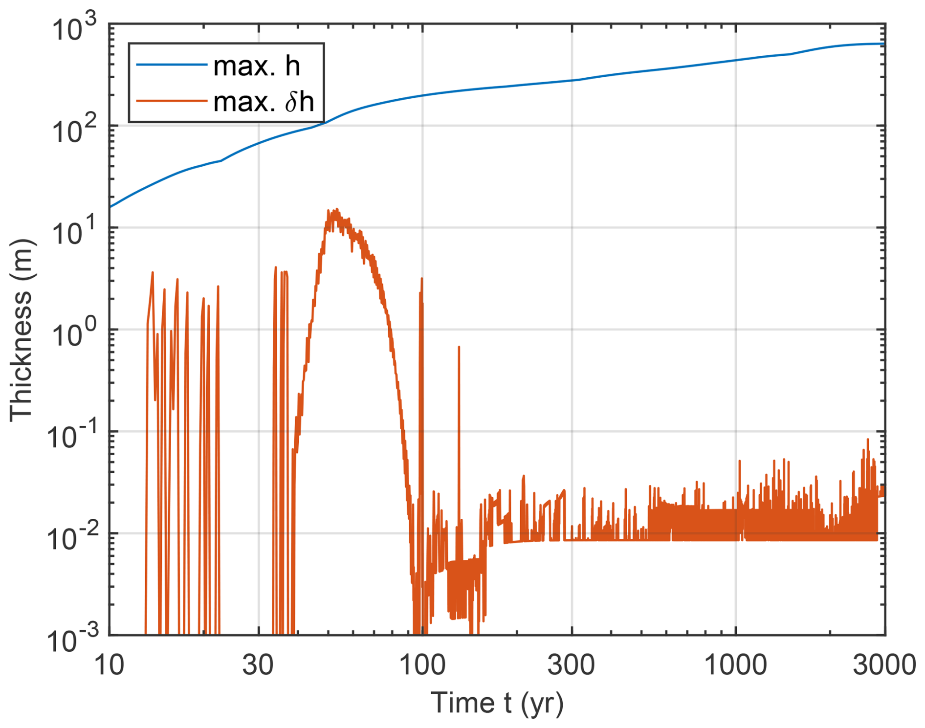
Figure 10 Maximum ice thickness h and maximum oscillation δh (Eq. 21) for δx=25 m and δt=0.25 years.

These oscillations are not a problem for the test scenario. Practically, it does not matter whether ice flows down steep slopes uniformly or in distinct surges, provided that the oscillations do not cause large errors in the volumetric balance due to negative values of h. In this example, the oscillations even cease for t>100 years due to filling up the steep slopes with ice. However, this is not necessarily the case for other topographies.

Some additional, but preliminary tests were performed for the Rhone–Aare region in Switzerland and the Salzach region in Austria as two examples of alpine topography. All parameter values were the same as for the Black Forest example, except for an ELA of z_e=1500 m and an upper limit for the net rate of ice production (Eq. 10) of $r_{max}=\mathrm{1}$ m yr⁻¹.

A time increment of $\mathit{\delta }t=\mathrm{1}/\mathrm{32}$ years turned out to be sufficient for both scenarios at δx=50 m, whereby the maximum ice thickness exceeded 2000 m in the Rhone–Aare example and 1450 m in the Salzach example. This time increment is 8 times smaller than that found for the Black Forest example. However, the maximum ice thickness is also more than 3 times higher and it was already found in Sect. 4.1 that the occurrence of staircase oscillations depends on ice thickness.

However, larger time increments caused oscillations of several meters at steep slopes already in an early phase of the simulation at moderate ice thickness. These oscillations cease in the Salzach example when the valleys have been filled with ice, which allows for increasing δt to $\mathrm{1}/\mathrm{16}$ years. This is, however, not the case for the Rhone–Aare example.

So the numerical efficiency is limited by the weak performance at steep slopes for moderate ice thickness in the alpine examples. Even increasing the ELA so that the maximum ice thickness is similar to that in the Black Forest example does not bring the maximum time increment close to the value $\mathit{\delta }t=\mathrm{1}/\mathrm{4}$ years achieved there.

Since the scheme is not much better than an explicit scheme concerning the dependence of the ice flux on h at steep slopes, the CFL criterion becomes relevant here in contrast to the results from the previous section. As mentioned above, the CFL criterion predicts a stronger (linear) dependence of the maximum δt on δx than found numerically for large ice thickness. Therefore, the limitation arising from steep slopes becomes more relevant with increasing spatial resolution.

As a consequence, simulations of large alpine regions with δx<50 m are hardly feasible on standard PCs. Beyond the limitation of the maximum time increment, the number of iterations of the PCG scheme also contributes to the increasing numerical effort. The results on the tolerance of the PCG solver found in Sect. 4.4 also hold for the alpine examples, whereby a tolerance of 10⁻⁵ even seems to be slightly better than in the Black Forest example. However, the absolute number of iterations is higher for the alpine examples. It even reaches 100 at h=2000 m, which lets the PCG solver contribute more than 80 % to the total effort.

However, the results obtained from the numerical tests still do not allow for estimating the maximum time increment from the topography and the parameters directly. Finding the maximum time increment experimentally by watching the maximum oscillation δh (Eq. 21) seems to be the best way to estimate the maximum δt at present.

6 Limitations of the SIA

While the numerical scheme proposed here introduces a major progress concerning the numerical efficiency, it cannot overcome the physical limitations of the SIA. As a main limitation, the SIA in the simple form considered here completely neglects stresses arising from horizontal shearing.

As an example, Fig. 11 shows the valley cross section marked in Fig. 1d. The valley is quite narrow here with a large ice thickness. The slope angles are about 30° and the depth-to-width ratio is higher than 0.25 and thus clearly not close to zero as theoretically assumed for the SIA.

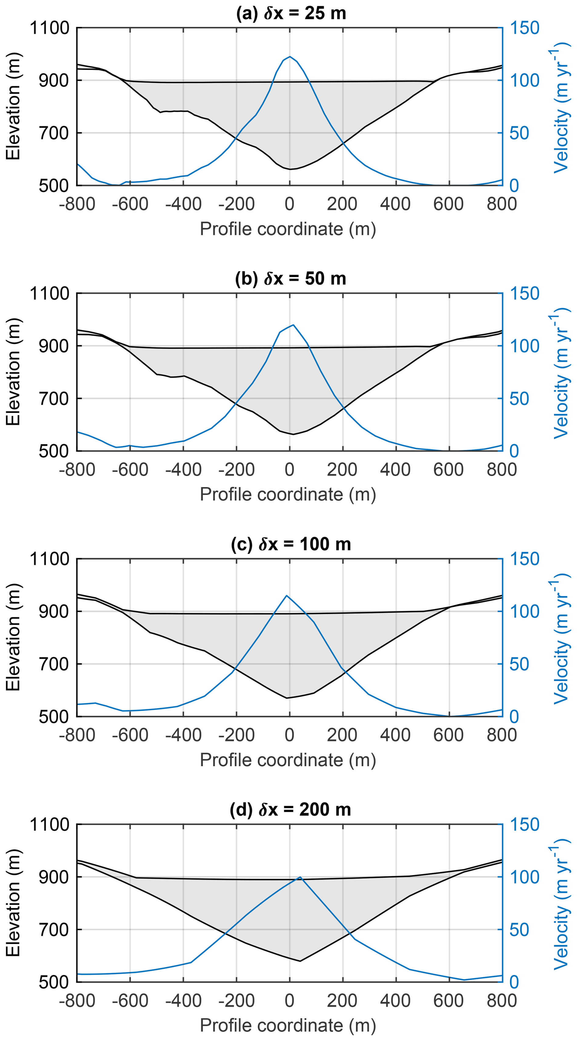
Figure 11 Cross section through the valley marked in Fig. 1d. Velocity is depth-averaged and includes deformation and sliding.

The simulated flow velocity is strongly concentrated around the center of the valley. The depth-averaged velocity decreases to half of its maximum value over a distance of about 150 m. In relation to a maximum thickness of about 300 m, this means that the horizontal velocity gradients are in the same order of magnitude as the vertical gradients. Accordingly, the horizontal shear stresses not captured by the SIA are in the same order of magnitude as the vertical shear stress and are by far not negligible.

In combination with the large ice thickness, the horizontal shear stresses would slow down the flow strongly in the central region. In turn, the horizontal stresses exert a driving force to regions of low velocity and thus increase the velocity there. Furthermore, these stresses increase the fluidity of the ice according to the nonlinear flow law. So the SIA overestimates the velocities in the central part of the valley and vice versa.

As shown in Fig. 11, neither the ice surface nor the velocities depend strongly on δx at least for δx≤100 m. The variations in the elevation of the ice surface at the center are a few meters, in agreement with the overall deviations analyzed in Fig. 8. In combination with the strong effect of horizontal stresses, the moderate dependence of thickness and velocity on δx shows, however, that we are already in the regime where the physical error of the SIA dominates over the numerical error.

The artificial concentration of high velocities around the center of the valley would be a crucial issue in glacial erosion models that assume that the erosion rate depends on the local sliding velocity (e.g., Braun et al., 1999; Egholm et al., 2012). Here it would even generate narrow canyons instead of U-shaped valleys, and their width would depend on the spatial resolution. In turn, the effect on reconstructions of ice margins might be smaller since the errors in flow velocity compensate partly and small changes in ice thickness have a large effect on the ice flux. So it depends strongly on the application how far the SIA can be pushed outside its theoretical range of validity, defined by the ice thickness being much smaller than the length scale of horizontal variations.

While the physical deficiencies of the SIA obviously limit the merit of spatial resolutions much finer than the width of steep valleys, this is not necessarily the case for the entire topography. Figure 12 shows the profile through the highest peak marked in Fig. 1d. The ice thickness is much smaller than the horizontal scale of the major topographic structures in the central part (e.g., 18 m at the highest peak and 7.7 m at the minimum). Since either the thickness is low or the spatial variation in velocity is moderate in each part of the profile, horizontal stresses should not have a major effect here. So the limitations of the SIA should not be crucial here.

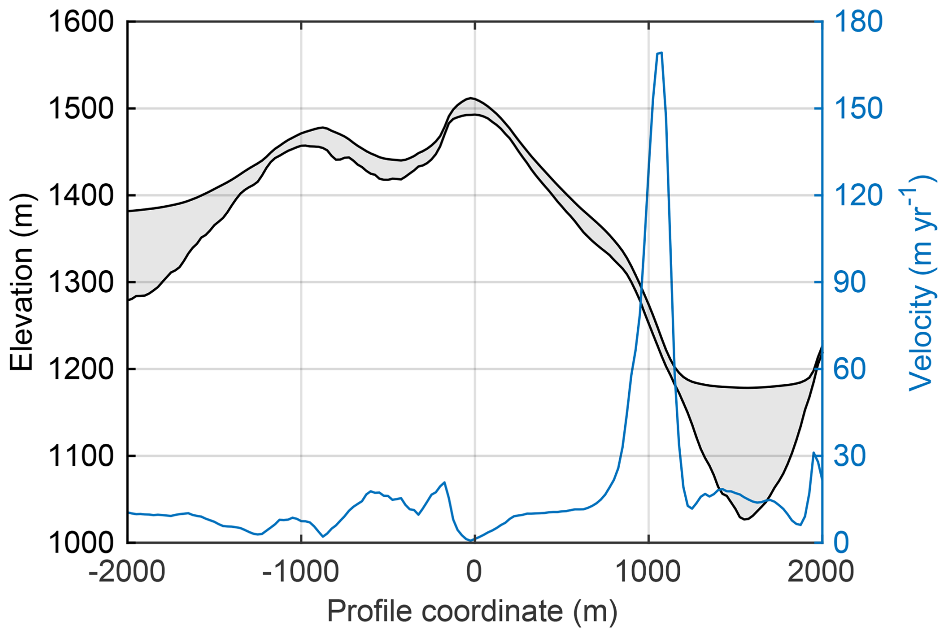
Figure 12 Cross section through the highest peak marked in Fig. 1d with a fivefold vertical exaggeration. Velocity is depth-averaged and includes deformation and sliding.

In any case, it would be desirable to include horizontal stress components. It is, however, not trivial whether any of the existing approaches (a second-order approximation or a combination with the shallow shelf approximation) could be implemented in such a way that the numerical efficiency is preserved or whether a different approximation is needed.

7 Software description

At present, MATLAB and Python implementations of MinSIA are available under the GNU General Public License. None of them requires specific packages, except for NumPy and SciPy for the Python version.

For performance reasons, the PCG solver and the incomplete Cholesky preconditioner used in the Python version were written in C++. Depending on the operating system, the C++ code (pcg.cpp) has to be compiled and the respective shared object file (pcg.so) should be placed in the same folder as the Python package (minsia.py). The respective dynamic-link library for Windows systems (pcg.dll) can be directly downloaded instead of compiling the source code.

Developers are encouraged to include and test alternative solvers for the linear equation system, which typically consumes the biggest part of the computing time. In particular for the Python version, it is recommended to include alternative solvers at the location of the direct solver in the code since the sparse matrix and the right-hand side of the equation system are easily recognized there. Improving the performance further by GPUs may be one option. It should, however, be noted that the standard PCG solver of SciPy was by up to 20 times slower than the compiled C++ version in the tests, which may reduce the improvement achievable by parallel computing strongly.

The implementation is minimalistic and consists of a class minsia (MATLAB) or MinSIA (Python), which contains only a constructor and a method step for performing a forward time step. Data handling and visualization are left to the user.

The constructor requires 4 mandatory arguments:

• An array b for the topography b.

• The grid spacing dx (δx=δy).

• The ice flow parameters fd (f_d) and fs (f_s). These parameters must be either scalar values or arrays with the same size as b.

Further optional arguments are:

• The model for the net rate of ice production prod, either given as an array with up to 3 elements or as a function handle. A 3-element array defines the accumulation gradient g₊, the ablation gradient g₋, and the maximum rate r_max (in this order) for the ELA-based model (Eq. 10). A 2-element array corresponds to $r_{max}=\mathrm{\infty }$ and a scalar value additionally to $g_{-}=g_{+}$. If prod is a function handle, it must refer to a function that receives the actual elevation s of the ice surface and the ELA z_e as arguments (so prod = @(s,ela)... or prod = lambda s,ela:...) and returns the net production rate r. It must be able to handle array-valued arguments. If the argument prod is not used, the production rate must be defined in each time step by the respective argument prod of the method step.

• The scalar smoothing factor f (f). Based on the findings of Sect. 4.1, the default value is f=1.

• A logical variable slopecorr that defines whether or not the correction for steep slopes (terms with cos β in Eqs. (3), (6), and (9)) are used. Default is true.

• The relative tolerance tol of the PCG solver. The default value is 10⁻⁷, which is a very conservative setting according to the findings of Sect. 4.4. A value of 10⁻⁶ should not affect the accuracy strongly and should improve the performance by about 10 %. Values higher than 10⁻⁵ are not recommended. Setting the tolerance to zero switches to a direct solver.

• The diffusivity diffus for custom models of ice flow according to Eq. (7). It must be a handle to a function that receives the ice thickness h, the slope of the ice surface $\left|\mathrm{\nabla }s\right|$, and the flow parameters f_d and f_s as arguments (so diffus = @(h,slope,fd,fs)... or diffus = lambda h,slope,fd,fs:...). It must be able to handle array-valued arguments.

The method step requires two out of the following three arguments:

• The time increment dt (δt) is strictly required. Since the occurrence of staircase oscillations depends on topography, ice thickness and flow parameters, it is not possible to provide a useful default value. It is instead recommended to watch the maximum oscillation and adjust δt manually. According to the preliminary tests, it is suggested to start the search somewhere around δt=0.1 years.

• A scalar value or an array ela (z_e) that defines the ELA.

• An array prod that defines the net rate of ice production (r) in each cell. If this argument is provided, the argument ela is not used.

The method step updates the thickness h. It returns the maximum oscillation (Eq. 21) and the ice volume that was added to compensate negative thickness values (Sect. 4.3). It also updates the class variable slope, which contains the smoothed slope of the ice surface, |∇s|^smoothed (Sect. 3.3). This property may be useful for calculating velocities. Furthermore, it updates the class variable dh, which contains the oscillation at each node (Eq. 21). This property may be helpful for analyzing oscillations in detail.

MinSIA assumes homogeneous Neumann boundary conditions, i.e., closed boundaries. If ice reaches the boundary, it will accumulate. Alternatively, Dirichlet boundary conditions, i.e., a given ice thickness, can be mimicked by setting the thickness to the requested value after each time step.

8 Summary and outlook

This paper presents a novel numerical scheme and a lightweight implementation of the SIA for the flow of ice over a given topography. Key features are a semi-implicit time-stepping scheme and a dynamic smoothing of the slope of the ice surface. The proposed scheme overcomes the limitations of explicit schemes at large ice thickness and small slopes, which are crucial to their numerical efficiency. The results of the performed numerical tests with grid spacings down to 25 m are promising.

Numerically, steep slopes are the main problem. In contrast to thick ice layers with moderately inclined surfaces, the new scheme is not much better than an explicit scheme for thin layers on steep slopes. This limitation depends on the topography and on the model parameters and becomes increasingly relevant for finer grids. Practically, some loss of performance was observed for steep alpine topographies at 50 m grid spacing. However, this loss does not affect the improvement compared to explicit schemes strongly.

Conceptually, the restriction to the SIA is the main limitation of the new scheme at present. Since the SIA neglects all horizontal stress components, it overestimates the flow velocities in the middle of valleys and vice versa. The SIA is also not well-suited if sliding along the bed is strong.

The physical limitation due to the restriction to the SIA is clearly stronger than the remaining numerical limitations. The new scheme allows for spatial resolutions that seem not to be achievable with conventional numerical models at a reasonable computational effort. In turn, however, such high resolutions are particularly useful in rugged alpine terrain, where the limitations of the SIA are most severe. At the moment, it has to be evaluated carefully how much the physical deficiencies of the SIA affect the respective application.

In this sense, challenging the hypothesis about the limited potential for further improvements in computational efficiency with classical numerical methods made by Jouvet et al. (2021) was partly successful. Numerical performance has been improved greatly, but only for a very simple model with clear physical limitations. Therefore, the approach developed here cannot compete with the Instructed Glacier Model (IGM) at present since the IGM achieves a high numerical efficiency without obvious limitations concerning the underlying physics.

Concerning the future development, the crucial question is whether horizontal stress components can be included to overcome the limitations of the SIA. If this is possible without losing much of the numerical efficiency, classical numerics may become competitive again to the IGM. It is, however, not trivial whether any of the existing approaches (a second-order approximation or a combination with the shallow shelf approximation) could be implemented in such a way that the numerical efficiency is preserved or whether a different approximation is needed.

Appendix A: The flux density for deformation

Let us, for simplicity, assume that the ice surface is parallel to the bed with a slope angle β and that the z-coordinate is perpendicular to the surface with z=0 at the bed. Then the shear stress acting on a surface-parallel plane is given by the downslope component of the weight of the ice column above z,

$$\begin{array}{}\text{(A1)}& \mathit{\tau }\left(z\right)=\mathit{\rho }g\sin \mathit{\beta }\left(\mathit{\kappa }-z\right)\end{array}$$

for $\mathrm{0}\le z\le \mathit{\kappa }$, where ρg is the specific weight of the ice and κ the thickness perpendicular to the surface. According to Glen's flow law, the strain rate is

$$\begin{array}{}\text{(A2)}& {\displaystyle \frac{\mathrm{1}}{\mathrm{2}}}{\displaystyle \frac{\partial }{\partial z}}{v}_{\text{d}}\left(z\right)=A\left(\mathit{\tau }\right(z){)}^n=A{\left(\mathit{\rho }g\sin \mathit{\beta }\left(\mathit{\kappa }-z\right)\right)}^n,\end{array}$$

where v_d(z) is the respective velocity and A the creep parameter (Pa⁻ⁿ s⁻¹). The velocity is then obtained by integration,

$$\begin{array}{}\text{(A3)}& \begin{array}{rl}{v}_{\text{d}}\left(z\right)& =\underset{\mathrm{0}}{\overset{z}{\int }}{\displaystyle \frac{\partial }{\partial \mathit{\zeta }}}{v}_{\text{d}}\left(\mathit{\zeta }\right)\mathrm{d}\mathit{\zeta }\\ & ={\displaystyle \frac{\mathrm{2}A{\left(\mathit{\rho }g\sin \mathit{\beta }\right)}^n}{n+\mathrm{1}}}\left({\mathit{\kappa }}^{n+\mathrm{1}}-{\left(\mathit{\kappa }-z\right)}^{n+\mathrm{1}}\right)\end{array}\end{array}$$

if A is constant. Integrating the velocity yields the flux density

$$\begin{array}{}\text{(A4)}& q_{\text{d}}=\underset{\mathrm{0}}{\overset{\mathit{\kappa }}{\int }}{v}_{\text{d}}\left(z\right)\mathrm{d}z=f_{\text{d}}{\left(\sin \mathit{\beta }\right)}^n{\mathit{\kappa }}^{n+\mathrm{2}},\end{array}$$

with

$$\begin{array}{}\text{(A5)}& f_{\text{d}}={\displaystyle \frac{\mathrm{2}A{\left(\mathit{\rho }g\right)}^n}{n+\mathrm{2}}}.\end{array}$$

Expressing κ in terms of the vertical thickness h according to κ=hcos β yields the relation

$$\begin{array}{}\text{(A6)}& \begin{array}{rl}{q}_{\text{d}}& =f_{\text{d}}{h}^{n+\mathrm{2}}{\left(\cos \mathit{\beta }\right)}^{n+\mathrm{2}}{\left(\sin \mathit{\beta }\right)}^n\\ & =f_{\text{d}}{h}^{n+\mathrm{2}}{\left(\cos \mathit{\beta }\right)}^{\mathrm{2}n+\mathrm{2}}{\left(\tan \mathit{\beta }\right)}^n,\end{array}\end{array}$$

which is the scalar version of Eq. (3) for n=3.

Appendix B: The flux density for sliding at the bed

Starting point is the relation

$$\begin{array}{}\text{(B1)}& v_{\text{s}}=k{\mathit{\tau }}^{\frac{n+\mathrm{1}}{\mathrm{2}}}{\displaystyle \frac{\mathit{\tau }}{\mathit{\sigma }-p}}\end{array}$$

(Cuffey and Paterson, 2010, Eqs. 7.11. and 7.17) for the sliding velocity v_s, where σ is normal stress and p water pressure. The term $k{\mathit{\tau }}^{\frac{n+\mathrm{1}}{\mathrm{2}}}$ describes the original relation proposed by Weertman (1957), whereby the factor of proportionality k depends on the thermal and mechanical properties of ice and on the roughness of the bed. The last multiplier in Eq. (B1) is the bed separation index introduced by Bindschadler (1983). According to Eq. (A1) for z=0, the shear stress at the bed is

$$\begin{array}{}\text{(B2)}& \mathit{\tau }=\mathit{\rho }g\sin \mathit{\beta }\mathit{\kappa }.\end{array}$$

For the normal stress, the component of gravity perpendicular to the surface must be taken into account, which yields

$$\begin{array}{}\text{(B3)}& \mathit{\sigma }=\mathit{\rho }g\cos \mathit{\beta }\mathit{\kappa }\end{array}$$

Inserting the stresses into Eq. (B1) yields

$$\begin{array}{}\text{(B4)}& v_{\text{s}}=f_{\text{s}}{\left(\mathit{\kappa }\sin \mathit{\beta }\right)}^{\frac{n+\mathrm{1}}{\mathrm{2}}}\tan \mathit{\beta }\end{array}$$

with

$$\begin{array}{}\text{(B5)}& f_{\text{s}}={\displaystyle \frac{k{\left(\mathit{\rho }g\right)}^{\frac{n+\mathrm{1}}{\mathrm{2}}}}{\mathrm{1}-\frac{p}{\mathit{\sigma }}}}.\end{array}$$

Then the flux density is

$$\begin{array}{}\text{(B6)}& \begin{array}{rl}{q}_{\text{s}}& =\mathit{\kappa }{v}_{\text{s}}=f_{\text{s}}\mathit{\kappa }{\left(\mathit{\kappa }\sin \mathit{\beta }\right)}^{\frac{n+\mathrm{1}}{\mathrm{2}}}\tan \mathit{\beta }\\ & =f_{\text{s}}{\mathit{\kappa }}^{\frac{n+\mathrm{3}}{\mathrm{2}}}{\left(\cos \mathit{\beta }\right)}^{\frac{n+\mathrm{1}}{\mathrm{2}}}{\left(\tan \mathit{\beta }\right)}^{\frac{n+\mathrm{1}}{\mathrm{2}}}\tan \mathit{\beta }\\ & =f_{\text{s}}{h}^{\frac{n+\mathrm{3}}{\mathrm{2}}}{\left(\cos \mathit{\beta }\right)}^{n+\mathrm{2}}{\left(\tan \mathit{\beta }\right)}^{\frac{n+\mathrm{3}}{\mathrm{2}}}\end{array}\end{array}$$

This equation is the scalar version of Eq. (6) for n=3.