Revisiting the parameterization of dense water plume dynamics in geopotential coordinates in NEMO v4.2.2

Based on an analytical study of the physics of dense overflow plumes, we suggest a new version of the bottom boundary layer parameterization of dense water plumes for geopotential vertical coordinates models. This parameterization is implemented in the NEMO ocean engine, based on a modification of the already existing tools to represent dense water plumes, and for the case of dense plumes that can be considered as geostrophic or quasi-geostrophic flows. A test case is designed to test the performance of the parameterization on a critical area of the North Atlantic Ocean, the Iceland-Scotland ridge, that includes the Faeroe Bank Channel. A comparison with the existing parameterizations already implemented in the NEMO ocean engine show that our approach increases the bottom density along the plume pathway. A sensitivity experiment of the different possible stages of this new parameterization shows their gradual effects. The addition of a downslope bottom pressure gradient term in the primitive equations is its most important feature to boost the bottom dense plume advection, although the parameterization of the downslope advection of the dense plume also contributes.

1 Introduction

Dense water plumes are an important feature of the global ocean circulation, which both supply dense water at various critical locations, and drive upper ocean circulation. Examples include plumes from the Antarctic slope, through the Strait of Gibraltar, and the broader Atlantic Meridional Overturning Circulation (AMOC) (Buckley and Marshall, 2016). The dynamics of oceanic circulation at the Iceland-Scotland Ridge, which here is used as a test case, plays a critical role in regulating the AMOC (Hansen et al., 2010) and, consequently, the marine climate in the northeastern Atlantic and the global climate system. The Faeroe Bank Channel (FBC) overflow, which is the coldest and densest water source for the AMOC (Larsen et al., 2024), becomes strongly modified by entrainment of ambient water masses within a short distance from the FBC-exit (Mauritzen et al., 2005; Ullgren et al., 2014). The confluence of the FBC plume and plumes from the weaker, more complex and less well monitored Iceland-Faeroe Ridge overflow (de Marez et al., 2024), produces the Iceland-Scotland Overflow Water, a key component of the deeper AMOC limb. Details of these overflows, their flow pathways, and complex entrainment processes are, however, not well understood, and pose major challenges for numerical ocean models. Since ongoing climate change is expected to impact this vital ocean system, there is a critical need to address these limitations.

Therefore, a proper representation of such dense overflows is necessary in ocean circulation models, including those using vertical geopotential coordinates such as NEMO (Madec and the NEMO system team, 2022), although the latest can also work using terrain following coordinates. Because of their staircase representation of the bottom, and because of the hydrostatic approximation, such models poorly represent overflows of dense water: any dense water mass that moves from a shelf towards a deeper region in a geopotential coordinates ocean model, will inevitably be at some point at the top of a water column, above water masses of lower density. At which point, since the hydrostatic assumption is equivalent to considering the vertical primitive equation as an only balance between density gradient and pressure, no resulting vertical velocity can be computed directly. Therefore, any hydrostatic ocean model will have no other choice than to mix down the water column, until it becomes stable, with denser water masses located below lighter ones only. What should be a downslope advection of dense water masses, that preserves the dense water mass characteristics, results therefore, in geopotential coordinates ocean models, in a mixing with downslope water masses. A consequence is that, in such models, dense water masses usually end their downslope journey with a bias regarding the depth that they are supposed to reach, reaching regions more shallow than observed.

In order to try to correct this issue, two parameterizations of the so-called “bottom boundary layer” (BBL hereafter) are used in models such a NEMO (Beckmann and Döscher, 1997; Campin and Goosse, 1999), referred respectively BD and CG hereafter. Such parameterizations aim at reproducing in geopotential coordinate models, the behaviour of sigma coordinates (or terrain following) models such as ROMS or BOM (Berntsen et al., 2023, 2024), for which the direct connection of grid cells along the bottom is a natural model feature. Although these parameterizations are relevant, their efficiency is not fully acknowledged in the literature, several numerical studies of dense overflows in numerical model consider that such parameterizations mix the dense plume more than they help its propagation (Colombo et al., 2020), and are sometimes referred with derogatory terms (Legg et al., 2006). Both BD/CG use methods that connect non-adjacent bottom grid cells, located at different depth, one that will be referred in the present article as the “shelf” grid cell, and another “deeper” one located down the shelf. The original BD parameterization is based on a coupling between a geopotential coordinates ocean model and a sigma coordinates sub-model to compute the bottom tracer changes in the BBL. However, they also provide a simpler approach, that only links shelf and deeper grid cells with a diffusion coefficient that is non-zero only if a downslope negative density gradient exists (end of Sect. 3c and Eq. 7, in BD), and it is only this approach that has been implemented in NEMO. When it comes to the implementation of CG in NEMO, it is close to that described in the reference article, with two notable exceptions though. First, the parameterization links shelf and bottom grid cells with an explicit volume and tracer flux in CG, whereas the NEMO implementation only creates a “virtual” link applied to tracers exclusively. Additionally, in the original parameterization of CG, it is implied that the downslope dense water advection can be tuned against the bottom slope, which is not the case in the NEMO implementation. The velocity of this flux is based on an empirical formulation linked with the density difference between shelf and deeper grid cells, and is non-zero only if a positive density gradient occurs between shelf and deeper areas. In NEMO, this velocity can also be replaced with the model's bottom velocity, with the extra restriction that this velocity must be orientated downslope. In the present article, we shall refer to the BD/CG parameterizations as their NEMO implementations, and not as the original versions described in the reference articles.

Our goal is to revisit these parameterizations to make them more consistent with the physics of dense water plumes which form the core of dense overflows, and show that this reformulation provides better results. In this framework, we mean that the purpose of a dense water plume parameterization should be to drive the plume along its observed pathway, and prevent it from mixing too rapidly with the ambient water masses, although we acknowledge it is quasi impossible in a z vertical coordinate model, to reach the quality of the dense water plume representation that could be achieved with a sigma-coordinates ocean model. We therefore define a better parameterization as one that permits the propagation of the dense water plumes along their observed pathway plume, and preserves their denser nature as much as possible. To reach this purpose, we distance ourselves from the assumptions of the BD/CG parameterizations, that consider either only that the plume downslope advection can be represented by a constant downslope diffusion coefficient, or that the dense plume velocity is that of the downslope bottom flow of the model, or that it is simply proportional to the downslope density gradient with a constant coefficient. We aim for a flexible parameterization, that takes into account the local plume physical characteristics. We base our new parameterization on an analytical study of dense water plumes (Wåhlin and Walin, 2001), and the conclusions of which have been confirmed by several experimental or numerical studies (Tassigny et al., 2024; Wirth and Negretti, 2022). We use as a test case NEMO based simulations of the Iceland-Faeroe-Scotland ridge, and more specifically of the dense overflows through the narrow Faeroe Bank Channel (FBC hereafter), and the Iceland-Faeroe ridge (IFR hereafter). For this purpose, we use the NEMO based regional configuration of Hordoir et al. (2022). A first section presents our strategy of parameterization and its implementation in NEMO, a second section presents a set of sensitivity experiments for the FBC and IFR region which shows that our parameterization provides better and more physically consistent results for this region. A third section discuses the results, and concludes this article.

2 Modifying and Improving BBL parameterizations

2.1 Dense Plume Advection Theory

We base our new parameterization on an analytical study of dense plume advection (Wåhlin and Walin, 2001). They represent a dense plume as a positive density anomaly located on a sloping bottom (Fig. 1), which can be described by a set of primitive equations (Eq. 1).

$$\begin{array}{}\text{(1)}& \begin{array}{rl}& {\displaystyle \frac{\partial u}{\partial t}}+u{\displaystyle \frac{\partial u}{\partial x}}+v{\displaystyle \frac{\partial u}{\partial y}}-fv=-F_x/h\\ & {\displaystyle \frac{\partial v}{\partial t}}+u{\displaystyle \frac{\partial v}{\partial x}}+v{\displaystyle \frac{\partial v}{\partial y}}+fu=-g^{\prime }{\displaystyle \frac{\partial }{\partial y}}(h-H)-F_y/h\end{array}\end{array}$$

in which h is the plume thickness, H is the depth, u and v are the h thickness-mean plume velocity components along the x and y axis respectively. f is the Coriolis parameter, F_x and F_y are friction terms along the x and y axis respectively, $g^{\prime }=g\mathrm{\Delta }\mathit{\rho }/{\mathit{\rho }}_{\mathrm{0}}$ is the reduced gravity related with the dense anomaly created by the plume. ρ₀ is the local ocean ambient density.

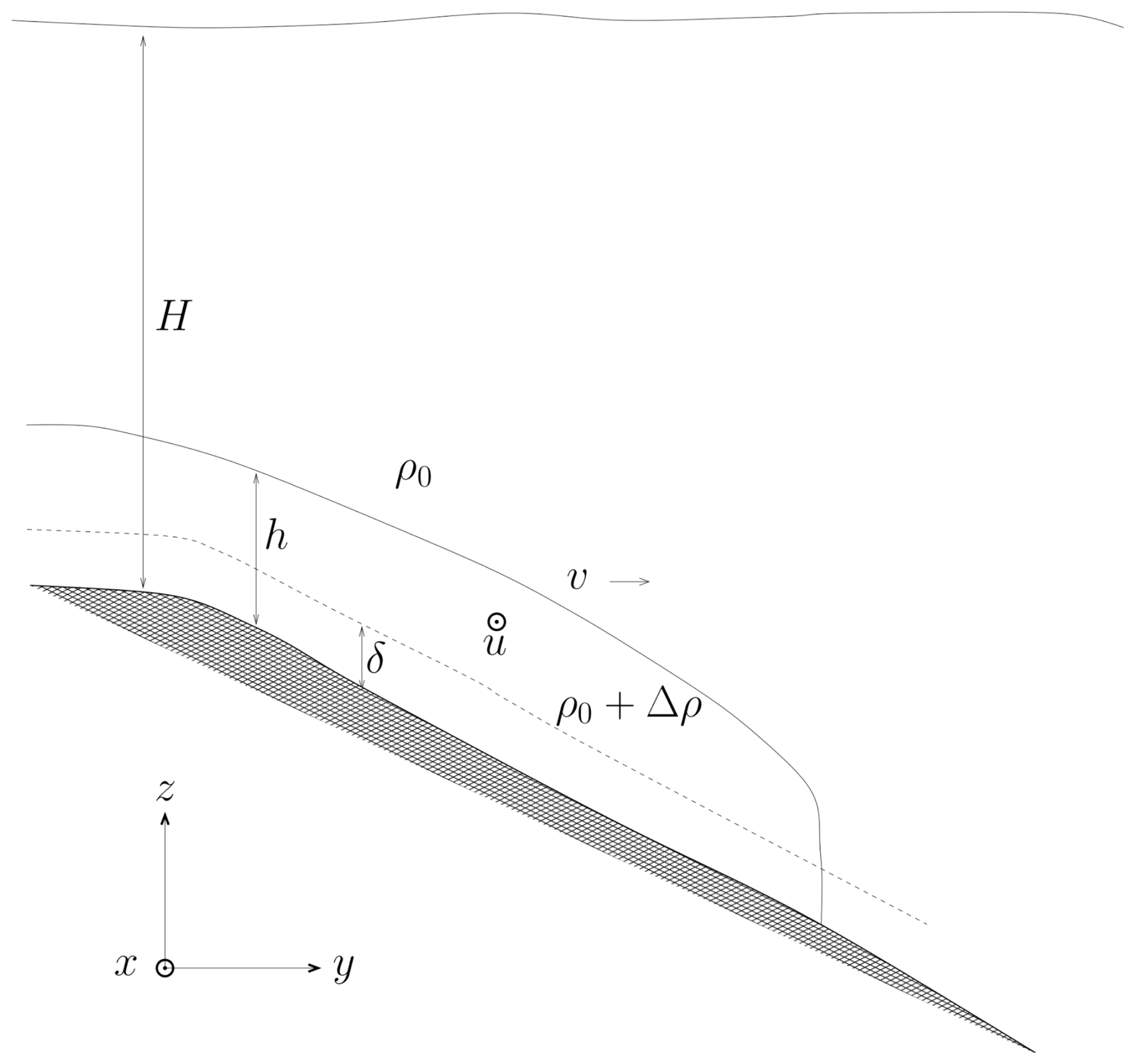
Figure 1 Following Wåhlin and Walin (2001), sketch of a dense plume advection located on a sloping bottom. h is the plume thickness, H is the depth, u and v are the h thickness-mean plume velocity components along the x and y axis respectively. δ is the thickness on which the plume friction effects occur. ρ₀ is the reference density, ρ₀+Δρ is the plume density.

Using dimensional analysis, Wåhlin and Walin (2001) show that the advection of a dense water plume moving along and down a slope (Fig. 1) can be represented with a simplified version of Eq. (1), as a set of quasi-geostrophic equations (Eq. 2). Wåhlin and Walin (2001) also consider a sub-thickness process in the friction layer δ which can create larger velocities than u, but since the size of δ is typically less than 10 m, we will consider it as a vertical subgrid scale process in our case, that can not be resolved, and consider only the h thickness-mean plume advection. Further results show that indeed, in our numerical simulations, δ≪h. Typical values of plume thicknesses h are of the order of 50 to 100 m (Wåhlin and Walin, 2001).

$$\begin{array}{}\text{(2)}& \begin{array}{rl}& -fv=-F_x/h\\ & fu=-g^{\prime }{\displaystyle \frac{\partial }{\partial y}}(h-H)-F_y/h\end{array}\end{array}$$

We define the alongslope geostrophic velocity u_g as:

$$\begin{array}{}\text{(3)}& u_{\mathrm{g}}={\displaystyle \frac{-g^{\prime }}{f}}{\displaystyle \frac{\partial }{\partial y}}(h-H)\end{array}$$

As in Wåhlin and Walin (2001), we compute $\mathit{\delta }=\frac{C_{\mathrm{D}}\left|u_{\mathrm{g}}\right|}{f}$, in which C_D is a dimensionless quadratic drag coefficient.

A linearisation of friction terms can be written as:

$$\begin{array}{}\text{(4)}& \begin{array}{rl}& F_x=C_{\mathrm{D}}\left|u_{\mathrm{g}}\right|u\\ & F_y=C_{\mathrm{D}}\left|u_{\mathrm{g}}\right|v\end{array}\end{array}$$

Equation (2) can be re-expressed as:

$$\begin{array}{}\text{(5)}& \begin{array}{rl}& v={\displaystyle \frac{\mathit{\delta }}{h}}u\\ & u=u_{\mathrm{g}}-{\displaystyle \frac{\mathit{\delta }}{h}}v\end{array}\end{array}$$

from which the h thickness-mean alongslope u and downslope v plume velocity components can be computed as:

$$\begin{array}{}\text{(6)}& \begin{array}{rl}& u={\displaystyle \frac{u_{\mathrm{g}}}{(\mathrm{1}+{\mathit{\delta }}^{\mathrm{2}}/h^{\mathrm{2}})}}\\ & v={\displaystyle \frac{\mathit{\delta }}{h}}{\displaystyle \frac{u_{\mathrm{g}}}{(\mathrm{1}+{\mathit{\delta }}^{\mathrm{2}}/h^{\mathrm{2}})}}\end{array}\end{array}$$

From this analytical analysis, Wåhlin and Walin (2001) show that the alongslope advection velocity of the plume is of an order of amplitude higher than that of the downslope advection. Downslope advection that is the result of a balance between friction and geostrophy.

These results can only be partially transposed to an ocean model in order to reach a parameterization of the plume advection however, for two main reasons. First because they are valid only from a large scale point of view, Wåhlin and Walin (2001) neglect the advection terms of Eq. (1) to reach them, and such an approximation can only be made if these terms can be neglected when compared with the effects of planetary rotation. Although valid for most major overflows in the global ocean (Faeroe Bank Channel flow, Denmark Strait, Gibraltar etc.), such an approximation is not valid in the case of a coastal overflow such as that of a Fjord, where the effect of rotation is not as relevant, and where the width of the Fjord is most likely to be less than that of the Rossby radius corresponding with the baroclinic flow of the dense plume. Second, the analysis of Wåhlin and Walin (2001) considers the dense water plume as integrated over its width. And so would an ocean model which resolution is coarser than that of the plume's Rossby radius. But if the ocean model is set with a higher resolution, it shall consider the dense plume as an ensemble of grid cells, and in each grid cell, the advection terms of Eq. (1) could be impossible to neglect. For example, in cases such as Baltic Sea dense inflows (Hordoir et al., 2019), the plume density difference with the ambient water masses is related with a baroclinic Rossby radius that can be higher than the grid resolution.

In the present article however, for which the main modelling tool is a NEMO based ocean model which resolution is about 10 km (Hordoir et al., 2022), we will consider that we are always in the case in which the plume baroclinic Rossby radius is less than the grid resolution, a case which would also apply to most ocean models used for climate simulations. Therefore, the advection terms of Eq. (1) are a subgrid scale process from a horizontal point of view, and the integration of Eq. (1) over a grid cell, yields a system of quasi-geostrophic equations. We will consider the plume advection can be therefore described according to Wåhlin and Walin (2001) and Eq. (2). As an example, if we consider a dense plume of thickness roughly 100 m, and the maximum density anomaly of the test case considered hereafter, we then get a baroclinic Rossby radius of about 3.6 km. So the quasi-geostrophic dynamics start to be described with a grid cell resolution higher than 1.3 km.

2.2 Implementation

The implementation of the analytical analysis of Wåhlin and Walin (2001) requires making further assumptions when it comes to vertical space scales. The thickness h of the dense water plume considered in Eq. (1) is an input data of the problem. We consider that h is simply equal to the bottom resolution of the numerical model, keeping a form of consistency with the former parameterizations of BD/CG. Further, we keep the axis notation used in the analytical study, but at this stage it is important to understand that the x or y direction used in the analytical study are exchangeable with any direction used in the numerical model. As long as what stands for y is equivalent with the downslope direction in NEMO, and what stands for x is equivalent with the alongslope direction in NEMO, with the triplet ($x,y,z$) in which z is orientated upwards, corresponding with the right-hand rule in the Northern Hemisphere.

Once h is set, it becomes possible to compute the driving momentum term, which is the downslope pressure gradient of Eq. (2). We define it as $\frac{\partial P_{\mathrm{r}}}{\partial y}=-g^{\prime }\frac{\partial }{\partial y}(h-H)$. A term that simply does not exist in geopotential ocean models such as NEMO, as it is a pressure gradient that is not between adjacent grid cells, meaning that the very energy source of dense plume advection is absent. This extra source of momentum cannot be naturally computed by a geopotential vertical coordinates ocean model, but can be computed using the already existing features inspired by CG implemented in NEMO. We add this extra source of momentum to the hydrostatic pressure gradient. This addition is a source of momentum to the model, will produce a response of the model in terms of volume, heat and salt transport, but which should remain conservative from a tracer point of view since only momentum was added to the model as for an extra forcing term.

This first stage of parameterization is referred hereafter as DPLUME-PRGR. It is worth noticing that this first stage of parameterization can be generalized to any ocean modelling configuration, as it just adds to the model a source of momentum that should exist. Adding this source of momentum parallel to the downslope density gradient, is always rightly orientated, regardless of the configuration (i.e.: large scale circulation or fjord) or of its numerical resolution. Further, any diagnostic made on energy balance, will include the flux of pressure, or pressure anomaly (Hordoir et al., 2008). It will therefore naturally take into account the inclusion of the parameterisation from this early stage onward.

Table 1 Comparison of the different BBL parameterizations and of their implementations.

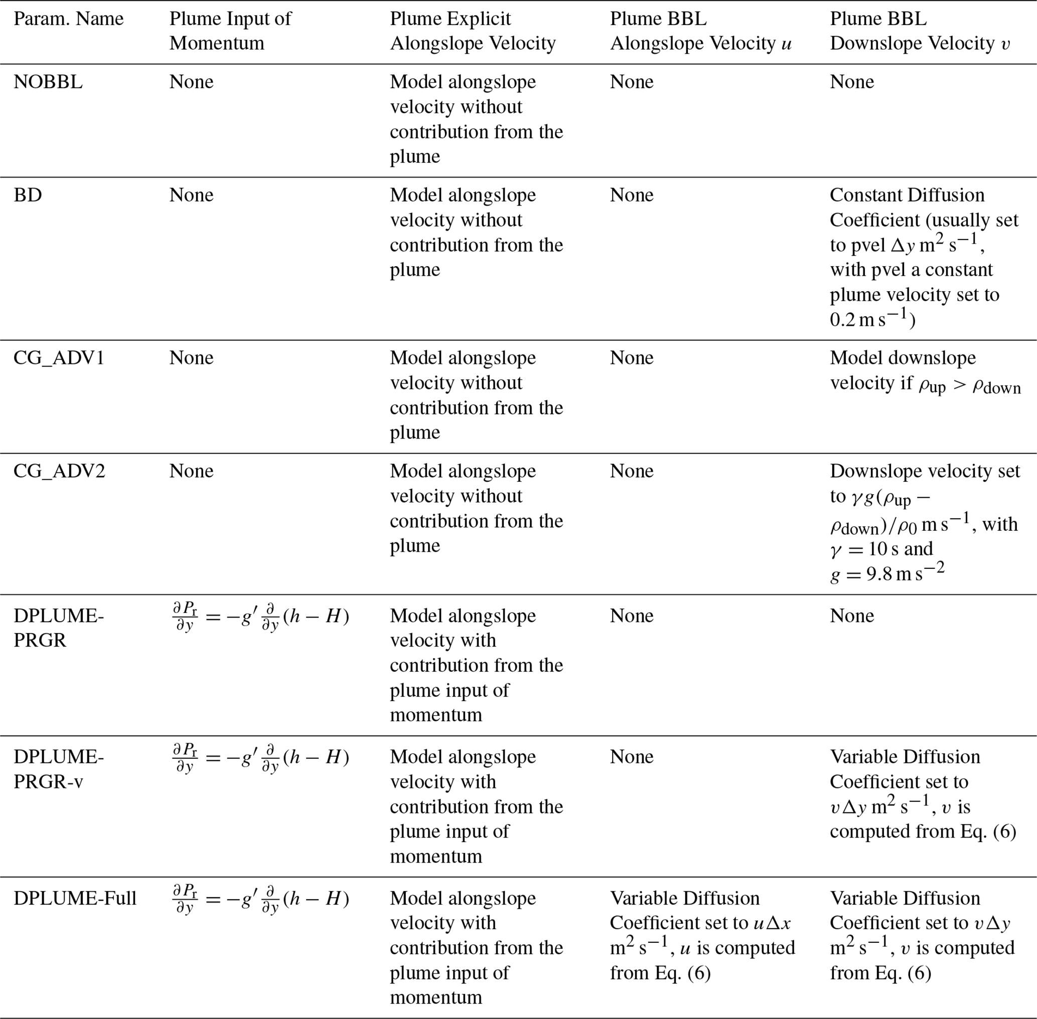
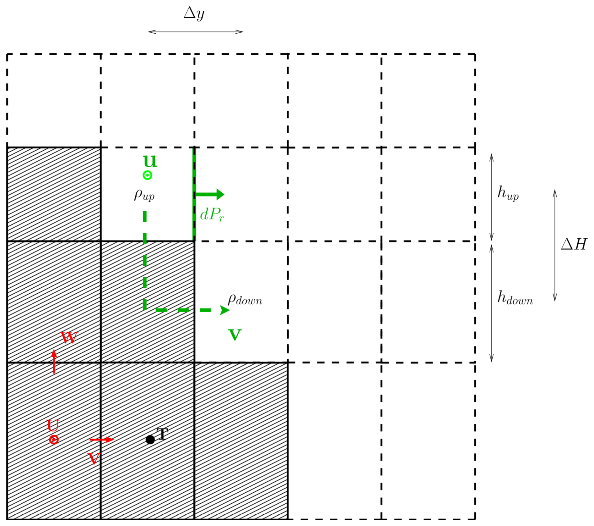
Figure 2 Numerical equivalent transposed on the Arakawa C-Grid of NEMO of the dense plume sketch of Fig. 1. The lower-left corners show the location of the T, U, V, and W points of the Arakawa C-grid. If a shelf grid cell has a shelf density ρ_up that is higher than the deeper density ρ_down, then at the shelf edge V point of the grid cell, an additional pressure gradient dP_r is added (Green Plain Arrow), and that is orientated horizontally towards deeper regions. Additionally, BBL velocities u and v of Eq. (6) are computed to be used for alongslope and downslope tracer advection between shelf and deeper grid cells, if such cells exist and if the addition is physically relevant.

The NEMO ocean engine solves the ocean dynamics primitive equations on an Arakawa C-Grid, for which a numerical sketch of a shelf break equivalent to that of Fig. 1 can be represented by Fig. 2. Using the model grid (Fig. 2), the additional downslope bottom pressure gradient is computed as

$$\begin{array}{}\text{(7)}& {\displaystyle \frac{\partial P_{\mathrm{r}}}{\partial y}}={\displaystyle \frac{g({\mathit{\rho }}_{\mathrm{up}}-{\mathit{\rho }}_{\mathrm{down}})}{{\mathit{\rho }}_{\mathrm{0}}}}{\displaystyle \frac{\mathrm{\Delta }H+(h_{\mathrm{up}}-h_{\mathrm{down}})}{\mathrm{\Delta }y}}\end{array}$$

in which the ρ_up, ρ_down, ΔH, h_up, h_down and Δy parameters are also represented in Fig. 2, and ρ₀ is the reference density. If a shelf grid cell has a shelf density ρ_up that is higher than the deeper density ρ_down, then $\frac{\partial P_{\mathrm{r}}}{\partial y}$ is non-zero. It is worth mentioning two points regarding Eq. (7), related with the use of partial steps for the description of bathymetry in an ocean model, as it will be illustrated hereafter. First, even if the thickness of the deeper grid cell h_down is more important than that h_up, the depth gradient term never becomes negative (and therefore unphysical). Due to the grid geometry, the bathymetry gradient ΔH is always higher than the gradient of grid cell thickness (h_up−h_down). Second, the bottom grid thickness h which we chose to coincide with the plume thickness, could appear to be too small compared with the observed plume thickness, due to the use of partial steps. From a practical point of view, this turns out to be true in shallow regions, where the vertical grid resolution is high. But in such regions, this high resolution also permits to limit the effect of steps on the mixing of overflows, which implies a BBL parameterization is not so relevant. In deeper regions, the bottom grid cell thickness in our experiments, turns out to be much larger and be close to the actual thickness of a dense water plume.

The addition of the extra pressure gradient $\frac{\partial P_{\mathrm{r}}}{\partial y}$ is made naturally at the V point of the Arakawa C-grid, as for any baroclinic pressure gradient (Fig. 2). Adding linearly this term to the hydrostatic pressure gradient creates a response of the model in terms of flow, especially close to the bottom as it will be shown hereafter, but this response is the addition of the dense plume effect to that of the local circulation. Adding this term should ensure, in a geostrophic or quasi-geostrophic case, to add the alongslope advection u of the plume to the model. As u is mostly a purely geostrophic velocity, and therefore mostly a linear response, we can consider that for small values of δ, adding the downslope pressure gradient results in adding u to the main flow. Indeed, computing δ based on the bottom drag coefficient corresponding with the bottom grid cell thickness, and the bottom roughness, shows that it is almost always an order of magnitude below that of the bottom grid cell thickness (usually below 10 %). In this case, u is not a sub-grid scale process from a vertical point of view, when it comes to considering the bottom grid cell as the plume thickness. This is not the case for the downslope advection v, that is a sub-grid scale process from a vertical point of view, generated by friction over the thickness δ of Eq. (6). v can therefore not be computed explicitly by the model as a result of the injection of the downslope pressure gradient. Injecting v directly as a volume flux, without violating volume or tracer conservation in the model could only be done if the total velocity components of the plume ($u,v,w$) were non-divergent, following for example the approach of Gent and Mcwilliams (1990). Such an injection is not suitable anyway, as v is the downslope velocity and should therefore connect the shelf grid cell with the deeper grid cell, and not with an adjacent grid cell. We therefore represent v as a tracer advection between bottom grid cells, following the approach of CG with v as a velocity linking those two grid cells, or v converted as diffusion coefficient following the approach of BD. We chose this later approach that we find produces better results. Adding the downslope v dense plume velocity as its equivalent in terms of downslope diffusion coefficient applied only to tracers, to the DPLUME-PRGR stage, defines a second stage of parameterization that we refer to as DPLUME-PRGR-v. When it comes to the alongslope velocity, computed by the model after the addition of the downslope pressure gradient, nothing forbids that the neighbouring alongslope grid cell is actually also downslope, meaning that the possibility of the alongslope transport to propagate higher density downward in that direction should also be considered. This is completed by adding the corresponding relevant diffusion between bottom grid cells in this direction too, also applied only to tracers. This can be done either by considering the local alongslope velocity computed by the model or the value of u computed from Eq. (6). Although consistent physically in terms of alongslope advection, we found that the resulting alongslope diffusion coefficients computed from the model bottom velocities reach high values that deteriorate the plume density. However, considering the u velocity for this purpose does improve results. Adding this contribution to the DPLUME-PRGR-v parameterization, defines a third and last stage of parameterization, referred as DPLUME-Full. We summarize the different stages of parameterization with their respective implementation, as well as the previously existing ones in NEMO in an array (Table 1).

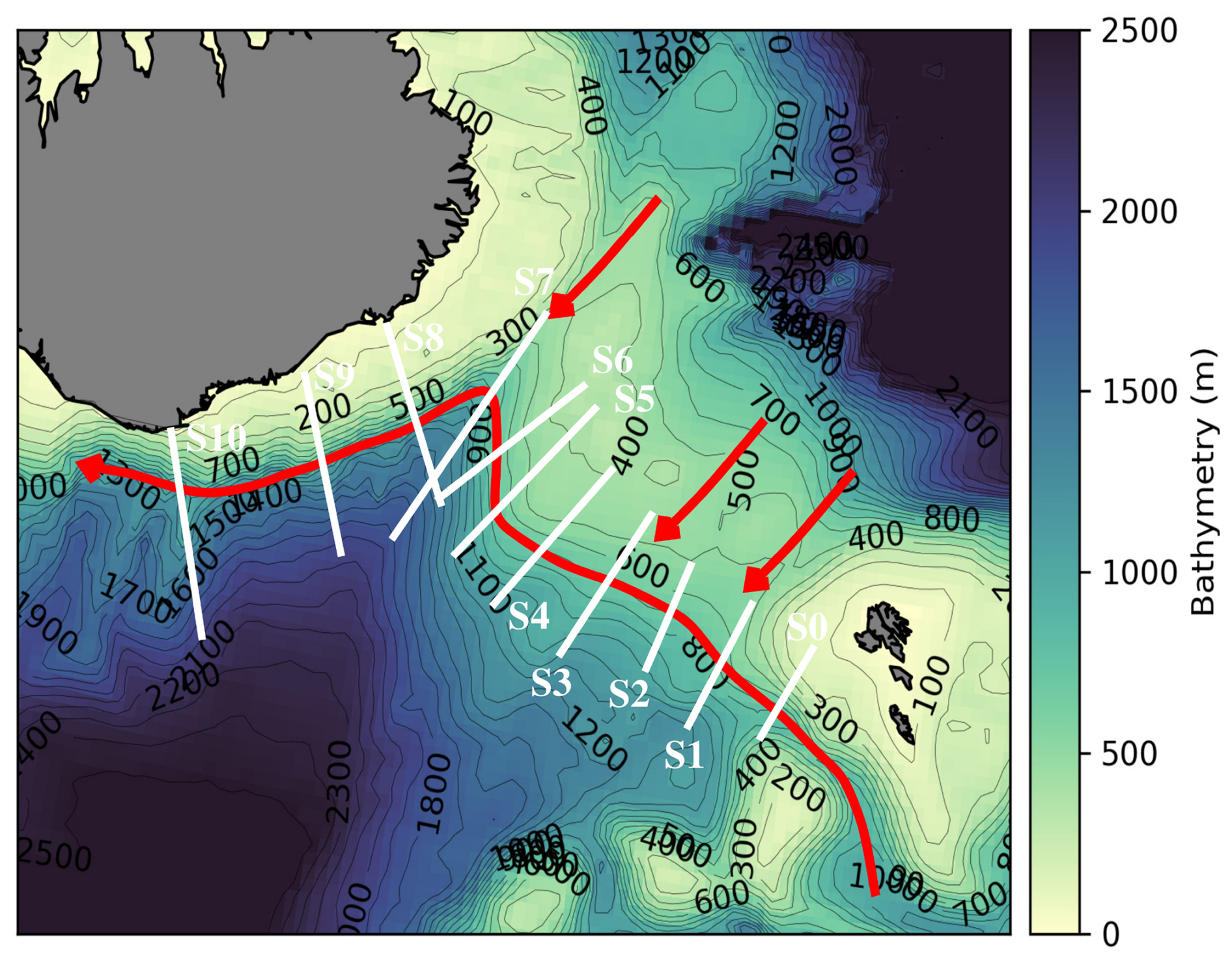
Figure 3 Bathymetry of the overflow region of the IFR and FBC. The red arrow shows the dense water pathway. Eleven sections (S0 to S10, white lines) are considered along the dense plume pathway, which propagates from FBC, get contribution across the IFR, and follows isobaths until it reaches the Southern Icelandic Shelf.

.

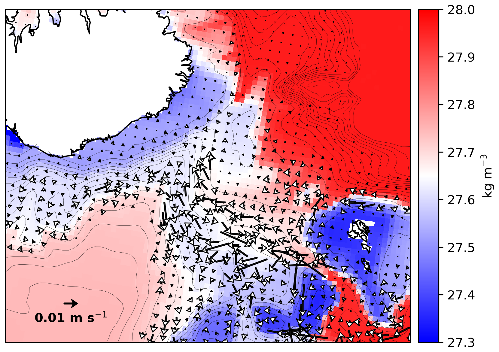
Figure 4 Vectors: Impact of the DPLUME-Full parameterization on bottom velocities, compared with the NOBBL reference. Comparison of bottom velocities EMO. Colourscale: NOBBL Bottom Density.

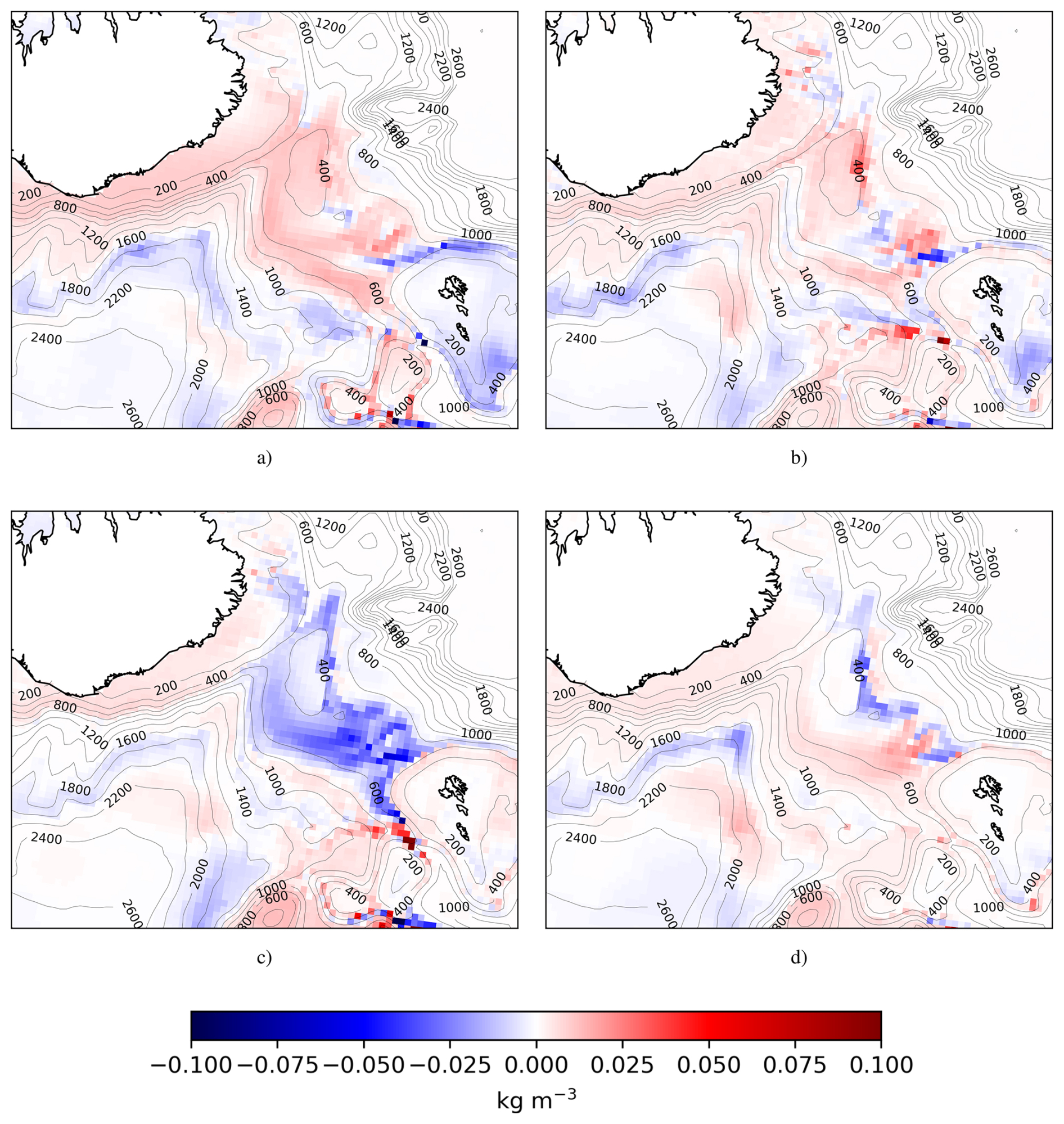
Figure 5 Comparison of bottom density between several BBL parameterizations. (a) DPLUME-Full minus NOBBL (b) BD minus NOBBL (c) CG_ADV1 minus NOBBL (d) CG_ADV2 minus NOBBL.

3 Comparison with Previous BBL Parameterizations and Sensitivity Experiment

Within the scope of this article, which is mostly to describe an alternative BBL parameterization, we did not test its effects based on a long term simulation. As a complete analysis of such a simulation would be out of the scope of this article, we instead use a test case to show the short term effects of the parameterization, and compare it with the previously implemented BD and CG parameterizations.

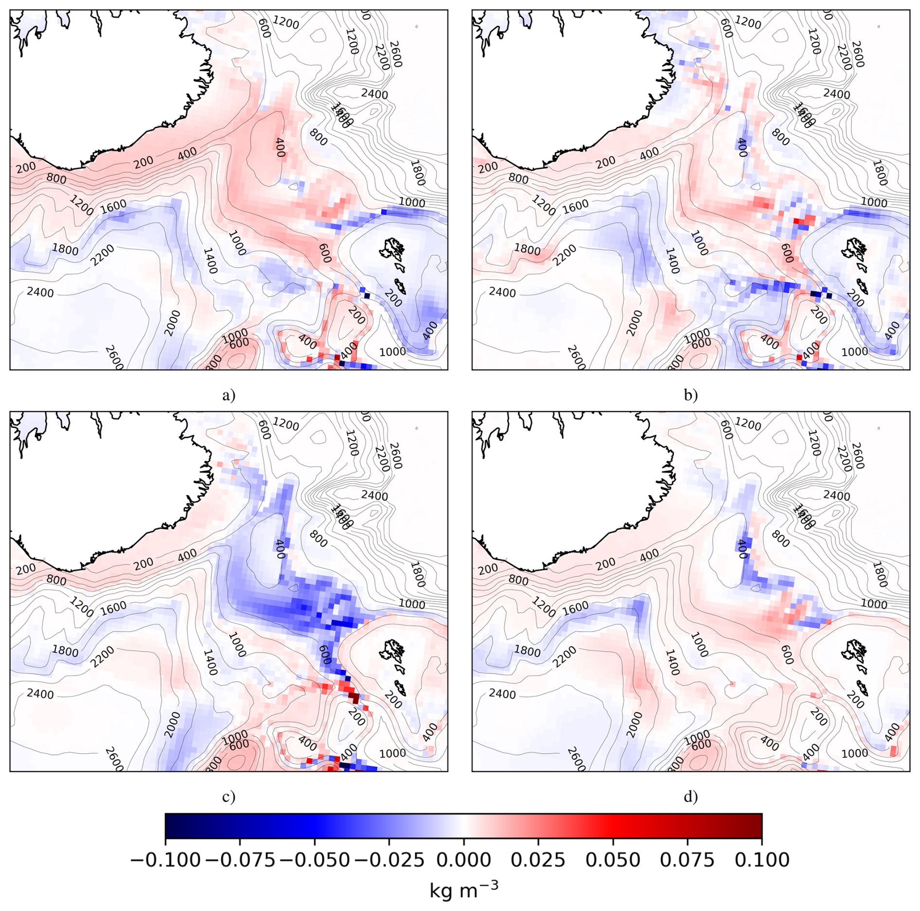
Figure 6 Comparison of bottom density between the DPLUME-Full parameterization with previously existing BBL parameterizations of NEMO. (a) DPLUME-Full minus NOBBL (b) DPLUME-Full minus BD (c) DPLUME-Full minus CG_ADV1 (d) DPLUME-Full minus CG_ADV2.

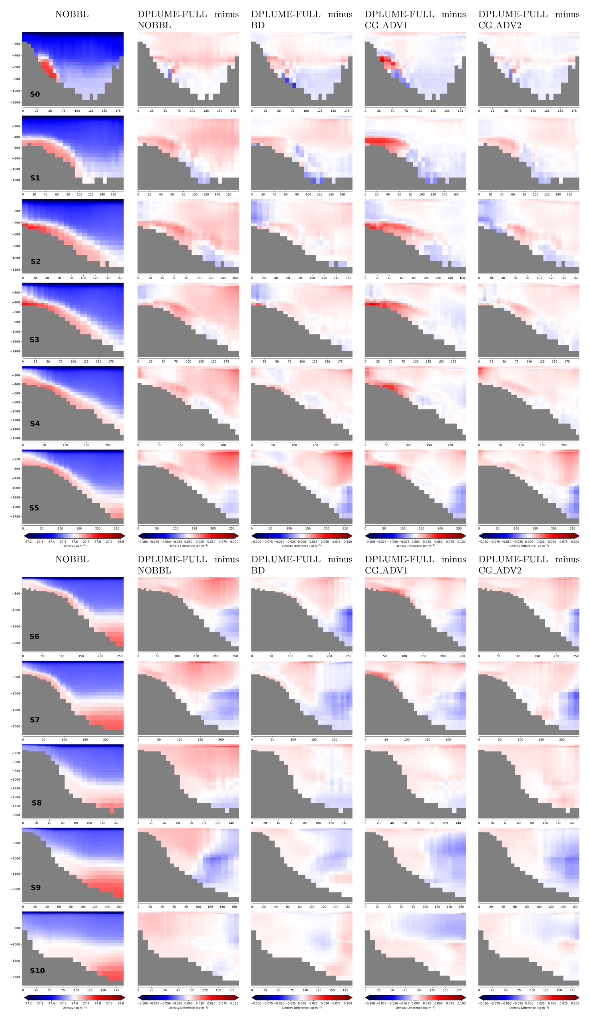
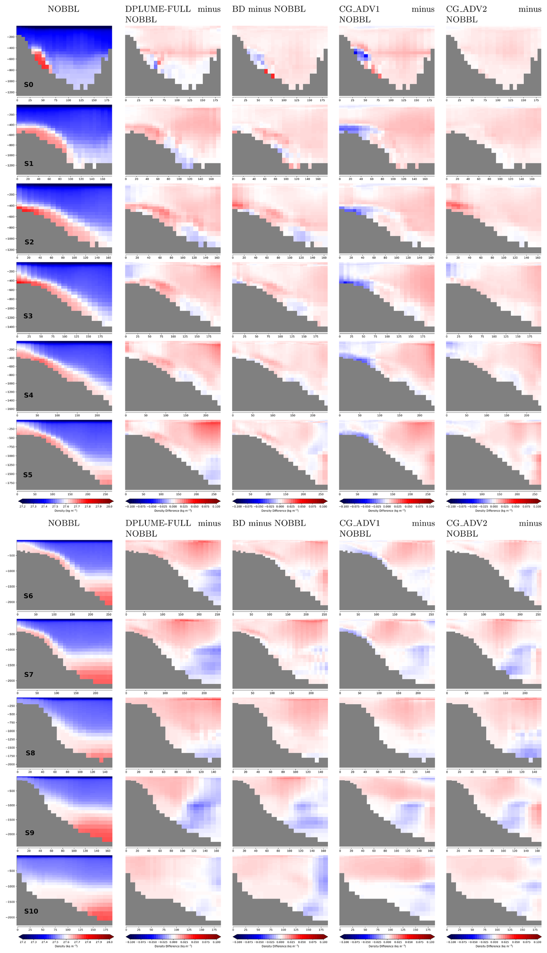
Figure 7 Comparison of density for the existing BBL parameterizations implemented in NEMO, based on BD/CG, with the DPLUME parameterization introduced in the present article. The cross-sections numbered 0 to 10 are that of Fig. 3. The vertical units are m (meters), and the horizontal units are km (kilometres).

3.1 The Iceland-Scotland Ridge Test Case

We consider the overflow region of the Nordic Seas to the Northern Atlantic of the IFR and FBC (Fig. 3). Along the dense plume pathway considered (Red Arrows in Fig. 3), the FBC sill is located before section S0. The dense water plume mixes with ambient water at the sill location, then follows isobaths, and gets dense water contributions from other sills located along the IFR. Considering the density anomaly of the dense plume at section S0, we compute that the plume baroclinic Rossby radius is about 3.6 km, suggesting the resolution required to resolve the quasi-geostrophic equations of the dense plume is more precise than 1.3 km. The numerical configuration that is to be used has a resolution of about 10 km at the location of IFR/FBC, which makes the plume can not be resolved from a quasi-geostrophic perspective, even where it exerts its strongest density gradient.

We consider a 3 year hindcast simulation of the Hordoir et al. (2022) configuration, for the period 1974–1976. The simulation starts from a restart file, and has been spun up for a long time period before 1974, with no BBL parameterization. From 1974 onward, the different parameterizations are activated, and we consider mean values of year 1976 to visualize results. We consider four reference simulations. One without any BBL parameterization (referred as NOBBL hereafter), one with a diffusive BBL following BD, one with an advective BBL following CG for which the advection velocity is the local bottom velocity if the flow goes downslope (referred as CG_ADV1 hereafter), and one for which the advection velocity is proportional to the density gradient (referred as CG_ADV2 hereafter). The different parameterizations are summarized in Table 1. We compare the effect of our DPLUME-Full parameterization on bottom density in the IFR/FBC region, with each of the four simulations. We also visualize the effects of the previously available parameterizations for comparison. Adding a source of momentum increases bottom velocities along the direction of propagation of the dense plume (Figs. 3 and 4).

A comparison of the DPLUME-Full parameterization with the previously existing parameterizations, shows that DPLUME-Full keeps the dense plume more concentrated, and propagates the positive density anomaly further along the plume pathway (Figs. 5 and 6). Taken individually, the BD, CG_ADV1 and CG_ADV2 parameterizations do increase the bottom density of the plume in certain locations, although the CG_ADV1 parameterization also destroys totally the overflow over the IFR ridge, but this increase is diffused and limited (Fig. 5). The DPLUME-Full parameterization advects dense water along the slope, which creates a negative anomaly just after the FBC sill, compared with the other parameterizations (Fig. 6). Compared with all the parameterizations previously implemented in NEMO, our DPLUME-Full parameterization produces the most consistent increase of bottom density along the dense plume pathway.

Comparing the parameterizations along the dense plume pathway, presented in Fig. 3, provides a comparison of the DPLUME-Full parameterization for each cross-section (Fig. ). The plume location follows the shelf break and loses density, before it can not be distinguished from the density of lower layers of the North Atlantic Basin located Southward of the Icelandic shelf break, and of the IFR. This latest water mass is made of North Atlantic Deep Water (NADW), and is not linked with the density of the dense plume. For sections located after the sill, the DPLUME-Full parameterization produces a higher density increase at the location of the dense plume, than the BD, CG_ADV1 and CG_ADV2 parameterizations (Fig. ), although it produces a weaker density increase in deeper regions, which can be attributed to a lower downslope flux (Sects. S1 to S5). However, for Sects. S6 to S10, there is a density increase that is more consistent across the entire section. One notices that for each comparison, there is a density increase close to the surface, which can even be higher than the bottom increase. We attribute this increase to an indirect effect, as the deep density increases, this effect propagates by entrainment in the mixed layer, which increases thermal stratification during summer, hence blocking a warming of deeper water and therefore positive feedback of density increase. This effect can be also noticed if a comparison between the existing parameterizations and the NOBBL simulation is made (not presented here). From the point of view of the dense plume, the DPLUME-Full parameterization is the one that prevents most of the plume from mixing with the surrounding water masses, and insures its advection along its natural pathway.

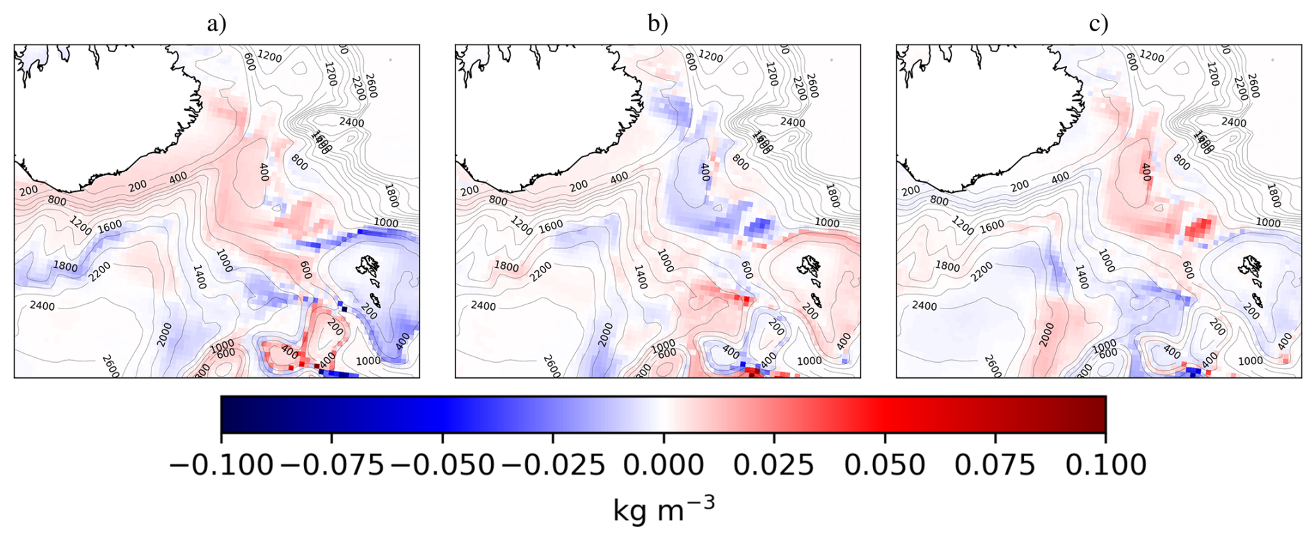
Figure 8 Difference of bottom density for the three stages of the DPLUME parameterization. (a) DPLUME-PRGR minus NOBBL (b) DPLUME-PRGR-v minus DPLUME-PRGR (c) DPLUME-Full minus DPLUME-PRGR-v.

3.2 Several Stages of Parameterization, a Comparison

It is relevant to assess the effect of the three different stages of the parameterization, in order to understand what are the physical processes that drive the plume's density increase created by the parameterization. Any increase of bottom density will result in an increase of the dense plume pressure gradient, and of u and v velocities, which makes the stages of the parameterization non-linear in terms of response. But it is still possible to compute the effect of each stage (Fig. 8). The most important effect is that of the addition of the downslope pressure gradient (Fig. 8a), which creates a consistent bottom density increase along the plume pathway, and a strong decrease downslope of the FBC sill, due to the increased alongslope advection that does not exist if the model runs with NOBBL, CG_ADV1 or CG_ADV2. Adding the v downslope velocity component, decreases the density at the location of the ridge line of the IFR, as denser water masses characteristics are diffused downslope, resulting however into a slight density increase further down. The last stage of the parameterization produces an additional density increase along the dense plume pathway.

4 Discussion and Conclusion

We suggest a refreshed and synthetic version of the parameterizations of BD/CG of dense water plumes. From a technical point of view, we used the tools already defined into the NEMO ocean engine, but reformulated the problem to make it more consistent with the physics of dense water plumes. The major addition of our parameterization is the addition of the downslope pressure gradient to NEMO, which is the momentum source of the motion of a dense plume. Inclusion which can never be unphysical regardless of the case considered (large scale circulation or fjord for example), or of the model's resolution. In the case of a quasi-geostrophic or geostrophic circulation, our parameterization uses diffusion coefficients to assess for downslope dense plume velocities as in BD, but whereas the parameterization of BD used a constant downslope diffusion coefficient, our DPLUME-Full parameterization computes diffusion coefficients which depend on the evolution of the dense plume anomaly, hence adapting the downslope diffusion to the dense plume dynamics. We show that this adaptation produces more consistent increases of bottom density. Further work is required however. First to adapt such a parameterization to the case of high baroclinic plume Rossby numbers. One can think of fjords for which the width of a fjord defines a space scale that limits the influence of geostrophy. But further, in the case we present (FBC and IFR dense overflow), the density difference is mostly a temperature related effect, that is limited at its very upper limit to 1 kg m⁻³, whereas the dense plume density of a fjord inflow is mostly generated by salinity gradient, which in a case of 10 to 15 PSU difference, may create larger density gradients (Arneborg, 2004). And therefore higher reduced gravity values g^′, and a higher dense plume baroclinic Rossby radius. It could also be the case of configurations such as the Black Sea Bosphorus salinity input (Gunduz et al., 2020), or that of the Baltic Sea (Hordoir et al., 2019), which present different circulation features for which the model resolution might enable a direct resolution of baroclinic eddies in the case of the plume. In this case our parameterization may not be relevant, at least for its DPLUME-PRGR-v and DPLUME-Full stages, but variations could easily be tested in which downslope velocities could be considered as being a full bottom grid cell process, instead of a sub-grid scale process related with a friction layer. We aim at testing such variations using the Baltic & North Sea NEMO configuration Nemo-Nordic (Hordoir et al., 2019). We also aim at testing long term effects of our DPLUME-Full parameterization over the entire Nordic Seas and Arctic Ocean, and study how it affects the renewal and export of Arctic dense water masses. Reaching a generalized version of the parameterization that would work regardless of the case is beyond the scope of this article, and so far it appears that final users should consider whether such a parameterization can apply or not, depending on the case considered. We conclude this article by mentioning a few technical points regarding the code and its computational efficiency. Our modified BBL parameterization is based on the existing NEMO 4.2.2 code, but has not been yet optimized from a computational point of view. We estimate that using this new parameterization increases computational costs by more than 10 %, but believe improvements can be made so that this new parameterization is computationally lighter.

Appendix A: Effect of existing BBL parameterizations implemented in NEMO, based on BD/CG and of the DPLUME-Full parameterization introduced in the present article

We provide in this appendix figures similar to Fig. , to show the effect of the BD, CG_ADV1 and CG_ADV2 parameterizations independently against a NOBBL simulation. For comparison purpose, we provide again in these figures the effect of the DPLUME-Full parameterization against a NOBBL simulation, as well as the NOBBL reference simulation.

Figure A1 The cross-sections numbered 0 to 10 are that of Fig. 3.