PM_2.5 assimilation within JEDI for NOAA's regional Air Quality Model (AQMv7): application to the September 2020 Western US wildfires

This paper describes efforts to establish aerosol data assimilation capabilities for NOAA's National Air Quality Forecasting Capability (NAQFC), a regional online air quality modeling (AQM) system under NOAA's Unified Forecast System (UFS), by assimilating measurements of fine particulate matter (PM_2.5, particles with aerodynamic diameters less than 2.5 µm). PM_2.5 assimilation is developed within the Joint Effort for Data assimilation Integration (JEDI) framework and tested using its 3D-Var data assimilation (DA) component. The PM_2.5 observation operator is constructed by combining newly developed PM_2.5 transformation recipes in the JEDI Variable Derivation Repository (VADER) with a general spatial interpolation operator in the Unified Forward Operator (UFO).

Cycled DA and forecast experiments were conducted from 1–21 September 2020, during a period of Western US wildfires, to assess the impact of assimilating PM_2.5 observations from the AirNow and PurpleAir networks. The control and analysis variables include individual aerosol species, with background error standard deviations generated by scaling their respective background values. Prognostic variables such as aerosol particle number and total particulate surface area are updated accordingly following each analysis update. All DA experiments use a 3-hourly cycling interval, with PM_2.5 observations assimilated every 3 h. The control experiment uses the same configuration but without any data assimilation. Results show that assimilating either AirNow or PurpleAir PM_2.5 data reduces 1–24 h forecast errors in terms of mean absolute error (MAE) and root mean square error (RMSE) compared to the control run over Continental United States (CONUS). Substantial improvements are in regions where fire events took place and largely affected by transported smoke. Overall, the assimilation of PurpleAir observations in addition to AirNow data leads to a slight reduction in 3–24 h MAE.

1 Introduction

Particulate matter with an aerodynamic diameter of 2.5 µm or smaller (PM_2.5) is a key contributor to poor air quality in the United States, posing significant risks to public health and the environment, and contributing to substantial loss of life (Cohen et al., 2017; Colmer et al., 2020; Huang et al., 2025). Over the past few decades, poor air quality in the US has contributed to over 100 000 premature deaths annually, far exceeding fatalities from all other weather-related causes combined, which average around 500 per year (Huang et al., 2025). Given its public health significance, PM_2.5 is one of the important pollutants used in calculating the Air Quality Index (AQI) – a standardized system designed to communicate daily air pollution levels to the public at the US Environmental Protection Agency (EPA). Elevated PM_2.5 concentrations frequently result in “unhealthy” AQI ratings, triggering health advisories and public warnings.

PM_2.5 in the United States originates from a range of both anthropogenic and natural sources. Anthropogenic sources include agricultural activities and combustion processes, such as emissions from motor vehicles, power plants, industrial facilities, and residential heating systems. Among natural sources, wildfires are a particularly significant contributor, especially in the western United States, where their frequency and intensity have escalated dramatically over the past two decades (Wen and Burke, 2021). According to the US Environmental Protection Agency (EPA), wildfires account for approximately 15 % to 30 % of total PM_2.5 emissions nationwide (EPA, 2017). While national seasonal averages of PM_2.5 have generally declined, summer PM_2.5 concentrations in the western US have remained persistently high, primarily due to wildfire smoke (O'Dell et al., 2019). In addition to degrading air quality, wildfires have caused widespread property loss. Since 2005, more than 129 000 homes, businesses, and other structures have been destroyed by wildfire-related events (https://headwaterseconomics.org/natural-hazards/structures-destroyed-by-wildfire, last access: 18 February 2026), underscoring the urgent need for more effective strategies in air quality monitoring, forecasting, and wildfire management.

The National Oceanic and Atmospheric Administration (NOAA) has developed an advanced regional Air Quality Modeling (AQM) prediction system within the Unified Forecast System (UFS) framework to enhance the accuracy of air quality forecasts across the United States, particularly during wildfire events (Huang et al., 2025). The National Air Quality Forecast Capability (NAQFC), operated by NOAA's National Weather Service (NWS), has been providing operational air quality forecast guidance for over 20 years, with continuous inclusion of new capabilities. Under NAQFC, the AQM version 7 was implemented and became operational on 14 May 2024. The system features online coupling of atmospheric and chemical models, allowing dynamic interactions between meteorology and atmospheric chemistry. This integration improves the representation of emissions and ensures real-time feedback of meteorological fields that influence chemical transformations and the transport of pollutants in the atmosphere. The UFS-AQM online system has consistently shown improved performance in simulating major wildfire events, including the significant wildfires in the northwestern coastal regions of the US in September 2020, and widespread smoke transport from Canadian wildfires in the summer of 2023. This system was officially implemented on 14 May 2024 as NOAA's operational air quality prediction system (AQMv7), replacing the previous offline-coupled Global Forecast System using the Finite Volume Cube-Sphere dynamical core (GFS-FV3) version 15 with the Community Multiscale Air Quality modeling system (CMAQv5.0.2) (Chen et al., 2021).

PM_2.5 data assimilation (DA) has proven effective in reducing errors in air quality forecasts (e.g., Pagowski et al., 2010, 2014; Schwartz et al., 2012; Wu et al., 2015; Robichaud, 2017; Sun et al., 2020; Lee et al., 2022; Chen et al., 2022; Ha, 2022; Park et al., 2022; Vogel et al., 2025, among others). Pagowski et al. (2010) demonstrated that fine aerosol forecasts benefit from AirNow PM_2.5 DA, showing improved verification scores for a period of at least 24 h. Schwartz et al. (2012) found that assimilating AirNow PM_2.5 observations significantly improved surface PM_2.5 forecasts over the CONUS compared to forecasts without DA. Wu et al. (2015) reported that incorporating ground-based PM_2.5 observations notably enhanced 24 h forecasts during a severe pollution episode in Shanghai. Similarly, Chen et al. (2022) showed that assimilating multi-source PM_2.5 data significantly improved WRF-Chem PM_2.5 forecasts with benefits lasting up to 48 h. Lee et al. (2021) highlighted the effectiveness of assimilating ground in-situ surface PM_2.5 observations in improving the short-term PM_2.5 predictions in Northeast Asia.

Many operational regional air quality prediction systems around the world use some form of data assimilation to initialize the forecasts. These approaches vary in complexity, ranging from simple optimal interpolation to full variational or ensemble Kalman filter methods (e.g. Robichaud et al., 2016; Wei et al., 2024; Colette et al., 2025). In NOAA's current regional air quality model (AQM) operations, aerosol and chemical initial conditions are “warm-started” using 6 h forecasts from the previous model cycle. The implementation of an aerosol data assimilation system can further enhance short-term air quality forecasts by providing more accurate spatial analyses of initial aerosol distributions.

To establish aerosol data assimilation capabilities for NOAA's regional operational AQM system, we employ the Joint Effort for Data assimilation Integration (JEDI) (Trémolet and Auligné, 2020). JEDI is a flexible, agnostic, and modern data assimilation system applicable to a wide range of forecasting systems (e.g. Liu et al., 2022; Huang et al., 2023; Sluka, 2024). JEDI offers a platform that supports efficient scientific development and facilitates the transition from research to operations. As part of a broader strategic shift, NOAA and partner agencies are transitioning their data assimilation systems to JEDI, opening the door for rapid integration of new scientific advancements, greater consistency across modeling systems, and enhanced collaboration across research communities and operational centers.

This study aims to develop and evaluate an initial aerosol analysis capability for the NOAA's regional AQM system by assimilating PM_2.5 observations using the JEDI three-dimensional variational (3D-Var) data assimilation framework. Compared to previous PM_2.5 data assimilation studies, this research adopts the NOAA's regional operational AQMv7 system and incorporates a new PM_2.5 transform in JEDI for assimilating PM_2.5 observations. In addition to evaluating the impact of assimilating AirNow PM_2.5 measurements on air quality prediction, this study also examines the impact of assimilating low-cost PurpleAir observations. Although PurpleAir data are valuable for PM_2.5 analysis (White et al., 2026) and real-time air quality monitoring, their potential impact on numerical air quality prediction remains insufficiently explored. To the authors' best knowledge, this is the first study to demonstrate the value of PurpleAir observations for air quality prediction during the wildfires of September 2020 using the AQMv7 system.

The paper is organized as follows: Sect. 2 provides a description of Methodology including the NOAA's AQM system, 3D-Var approach, and JEDI PM_2.5 assimilation. Experimental setup is presented in Sect. 3 including case description, AQM configuration, AirNow and PurpleAir PM_2.5 observations and background errors setup. Results are described in Sect. 4. A summary and discussion are presented in the final section.

2 Methodology

2.1 AQMv7 overview

The NOAA's regional operational AQMv7 system was developed through the online coupling of the Finite-Volume version 3 (FV3) dynamical core-based atmospheric model (Black et al., 2021) with the EPA's Community Multiscale Air Quality (CMAQ) model v5.2.0 within the UFS framework (Huang et al., 2025). In this UFS-AQM online system, CMAQ is treated as an atmospheric chemistry column model to simulate atmospheric chemistry reactions that govern concentrations of chemical species including gas- and aerosol-phase species. The transport terms of chemical species are handled by the FV3 dynamical core in the same way as other physics tracers (Huang et al., 2025). Aerosol module version 6 (AERO6) (Zhang et al., 2018) is utilized by CMAQ to simulate aerosol processes.

2.2 PM_2.5 assimilation within JEDI 3D-Var

In the JEDI framework, a series of components are provided to create a flexible, comprehensive data assimilation system (Trémolet and Auligné, 2020). The JEDI 3D-Var component is used to assimilate PM_2.5 for AQMv7. The 3D-Var method is chosen for its operational feasibility, primarily due to its low computational cost and the fact that it does not require an ensemble prediction system, as is needed in (hybrid) ensemble–variational data assimilation.

In practice, a 3D-Var data assimilation system typically uses an incremental approach to minimize a quadratic cost function which is defined in terms of the analysis increment δx relative to the guess state x_g:

$$\begin{array}{}\text{(1)}& \begin{array}{rl}J\left(\mathit{\delta }x\right)=& {\displaystyle \frac{\mathrm{1}}{\mathrm{2}}}(\mathit{\delta }x-\mathit{\delta }{x}_{\mathrm{g}}){\mathbf{B}}^{-\mathrm{1}}(\mathit{\delta }x-\mathit{\delta }{x}_{\mathrm{g}}{)}^T\\ & +{\displaystyle \frac{\mathrm{1}}{\mathrm{2}}}\left(\mathbf{H}\right[\mathit{\delta }x]-\mathit{d}){\mathbf{R}}^{-\mathrm{1}}\left(\mathbf{H}\right[\mathit{\delta }x]-\mathit{d}{)}^T\end{array}\end{array}$$

Where:

• $\mathit{\delta }{x}_{\mathrm{g}}=x_{\mathrm{b}}-x_{\mathrm{g}}$ is the guess state departure from background state, which is usually taken from a previous short-term forecast.

• H is the linearized observation operator of nonlinear observation operator H.

• B and R are the background and observation error covariance matrices, respectively.

• d is the innovation vector, defined as:

$$\begin{array}{}\text{(2)}& \mathit{d}=\mathit{y}-H\left(x_{\mathrm{g}}\right)\end{array}$$

with y representing the observation vector.

Once the increment δx is obtained, the analysis state x_a is reconstructed as:

$$\begin{array}{}\text{(3)}& x_{\mathrm{a}}=x_{\mathrm{g}}+\mathit{\delta }x\end{array}$$

2.2.1 PM_2.5 observation operator

To assimilate PM_2.5 data, a PM_2.5 transform that builds relationships between the model aerosol variables and the observed PM_2.5 needs to be developed. In AQMv7, the modal approach taken in the CMAQ model represents aerosol particle size distributions as the superposition of three lognormal modes: Aitken (I), accumulation (J), and coarse (K). It predicts only three integral properties of the size distribution for each mode: the total particle number concentration, the total surface area concentration, and the total mass concentration of the individual chemical components.

The total PM_2.5 concentration is calculated as a weighted sum of the individual aerosol concentration across these three modes:

$$\begin{array}{}\text{(4)}& \begin{array}{rl}{\mathrm{PM}}_{\mathrm{2.5}}=& \text{ATOTI}\cdot \text{PM25AT}+\text{ATOTJ}\cdot \text{PM25AC}\\ & +\text{ATOTK}\cdot \text{PM25CO}\end{array}\end{array}$$

Here, ATOTI, ATOTJ, and ATOTK represent the total aerosol mass concentrations in the Aitken, accumulation, and coarse modes, respectively. For example, ATOTI is the combined mass of 14 prognostic aerosol variables in the Aitken mode from the AERO6 aerosol module. Similarly, ATOTJ and ATOTK are the aggregated mass concentrations of 49 and 7 aerosol variables in the accumulation and coarse modes, respectively. PM25AT, PM25AC, and PM25CO are mass scaling factors for the three modes that vary by location and time. The aerosol variables within the same mode share the same mass scaling factor.

The PM_2.5 observation operator is constructed by combining the newly developed PM_2.5 transformation recipes in the JEDI Variable Derivation Repository (VADER) with an existing general spatial interpolation operator in the Unified Forward Operator (UFO). VADER is responsible for transforming model variables using user-defined “recipes” to generate new variables in model space. For PM_2.5 assimilation, VADER computes PM_2.5 from individual aerosol species using model-specific transformation, specifically using the Eq. (4) for this application. Since PM_2.5 composition varies by model, these transforms are implemented within VADER to match the specific structure of the regional air quality model AQMv7. Once PM_2.5 is derived in model space, UFO applies a generic spatial interpolation operator to map the model-simulated values to the observation locations, enabling computation of the observed minus forecast values.

The inputs for the PM_2.5 transformation are mixing ratio of the 70 aerosol variables with respect to dry air, the three mass scaling factors in the three modes, and dry air density for unit conversion. The output is the PM_2.5 in unit µg m⁻³. It is noted that a new routine (recipe) has been added to VADER to derive dry air density from air temperature, pressure, and the specific gas constant for the dry air using the ideal gas law. This is applied in cases where the dry air density is not otherwise provided for the PM_2.5 calculation.

The new JEDI/VADER PM_2.5 recipe provides nonlinear (NL), tangent linear (TL), and adjoint (AD) transforms of PM_2.5 that keeps the output products in the same grid space as the input variables. Hence, the generic interpolation operator in UFO is used to connect the model-derived PM_2.5 fields with observed surface PM_2.5 measurements. This respects the JEDI paradigm of keeping the UFO component of the JEDI model independent.

2.2.2 Background error covariance modeling

In a 3D-Var system, the background error covariance (BEC) determines both the spatial spreading of information from observations, and the magnitude of the analysis increments along with the observation error variance.

The background error covariance matrix B can be decomposed into a standard deviation matrix (Σ) and a correlation matrix (C), as follows:

$$\begin{array}{}\text{(5)}& \mathbf{B}=\mathbf{\Sigma }\mathbf{C}\mathbf{\Sigma }\end{array}$$

The correlation matrix C is generally non-diagonal. Σ is a diagonal matrix, with the standard deviations of the background errors for each variable on the diagonal.

The error modeling of the correlation matrix and standard deviations usually apply to control variables. In the first implementation of aerosol data assimilation in JEDI for AQMv7, the control variables are defined as individual forecast aerosol variables, resulting in 70 control variables for AQMv7 with the AERO6 aerosol mechanism. The setup of background error standard deviation and correlation modeling will be described in Sect. 3: Experimental setup.

2.2.3 Minimization Algorithm (DRIPCG)

JEDI provides several minimization algorithm options. In this paper, we use the Derber–Rosati Inexact Preconditioned Conjugate Gradient (DRIPCG) algorithm (Derber and Rosati, 1989), as implemented in the JEDI's OOPS (Object-Oriented Prediction System) framework. DRIPCG has been extensively tested and is chosen here for stability and convergence efficiency.

3 Experimental setup

3.1 The September 2020 fire event and AQMv7 system setup

The wildfires of September 2020 ranked among the most intense in the US in recent years. These fires produced dense smoke that initially moved westward over the Willamette Valley in western Oregon and eventually blanketed the broader region. As a result, air quality rapidly across Oregon, Washington, and Idaho deteriorated to hazardous levels, marking one of the worst air quality periods in recent decades (Mass et al., 2022). Wildfire smoke originating from California, Oregon, and Washington was injected into the free troposphere and transported across the country by prevailing winds, leading to hazy conditions in several states. According to Li et al. (2021), from August to October 2020, wildfires in the western US contributed 23 % of surface PM_2.5 across CONUS, with higher contributions observed along the Pacific Coast (43 %) and in mountain region (42 %). This study focuses on the peak fire activity occurring between 1 and 21 September.

In this research, the model configuration is almost the same as the operational AQMv7 setup except for running over the CONUS domain with a 3-hourly cycling interval. The AQMv7 system is configured over the CONUS domain with a grid-spacing of 13 km and 65 vertical levels, extending up to 0.2 hPa. The system uses the Global Forecast System version 16 (GFSv16) physics package within the Common Community Physics Package (CCPP) framework to generate the meteorological fields driving air quality predictions. Meteorological initial conditions and lateral boundary conditions are generated using GFS forecast outputs with lead times up to 30 h at 3 h intervals from the previous GFS cycle. Fire-related emissions are represented using real-time Regional hourly Advanced Baseline Imager (ABI) and Visible Infrared Imaging Radiometer Suite (VIIRS) Emissions (RAVE) data at 0.03° spatial resolution. Anthropogenic emissions are based on the 2016 US EPA NEI Collaborative (NEIC2016v1) modeling platform. Gas-phase chemistry is simulated using the Carbon Bond Mechanism version 6 (CB6r3) with updated isoprene chemistry and revised photolysis rates. More detailed information including physics, chemistry options, anthropogenic emissions, and fire emissions about the model configuration can be found in Huang et al. (2025).

3.2 PM_2.5 observations

In this study, surface PM_2.5 observations were obtained from two sources: AirNow and PurpleAir observing networks. These datasets differ in sensor type, spatial coverage, and quality control (QC) requirements. AirNow provides regulatory-grade measurements from federal, state, and local monitoring stations, while PurpleAir is a low-cost, community-based network of air quality sensors. PurpleAir sensors are widely deployed by individuals and communities, providing real-time data on PM_2.5 concentrations as well as meteorological variables such as temperature, pressure, and relative humidity. Only the data reported from outdoor PM_2.5 sensors are used in this study. The PurpleAir data were available for registered users through the PurpleAir API (https://community.purpleair.com/t/api-use-guidelines/1589, last access: 18 February 2026).

3.2.1 PurpleAir PM_2.5 quality control

Quality control and correction of PurpleAir data followed the methodology described in Barkjohn et al. (2021). Readers are referred to that paper for further details. The following quality control (QC) filters were applied to the raw PurpleAir PM_2.5 measurements:

• Reported PM_2.5 values from two Plantower sensors within the PurpleAir sensor (channels A and B) must be nonnegative.

• The PurpleAir sensor channel A and B consistency:

  • –

    Absolute difference <5 µg m⁻³, or

  • –

    Relative difference within 61 %.

• PM_2.5 values must not exceed PM₁₀ values.

• PM_2.5 values must be less than 3000 µg m⁻³ (upper threshold).

• Gross check of relative humidity with range 0 %–100 %.

Only PurpleAir PM_2.5 measurements that passed all the above QC criteria were retained for subsequent correction.

3.2.2 PurpleAir PM_2.5 correction

A correction is required because the PurpleAir raw data usually overestimate PM_2.5 concentrations under typical ambient and smoke-impacted conditions. Correction of PurpleAir PM_2.5 measurements was performed using a multiple linear regression model based on sensor-reported PM_2.5 (PA) and relative humidity (RH), following the correction formula proposed by Barkjohn et al. (2021):

$$\begin{array}{}\text{(6)}& {\mathrm{PM}}_{\mathrm{2.5}}=\mathrm{0.524}\times \text{PA}-\mathrm{0.0862}\times \text{RH}+\mathrm{5.75}\end{array}$$

We adopt the above equation because it was United States-wide valid by fitting data from September 2017 until January 2020. In addition, although the correction was originally derived for 24 h averaged PM_2.5, it is consistent with a regression equation obtained from the September 2020 dataset based on 1 h averaged PM_2.5.

3.2.3 Observation error assignment

Observation error standard deviations were assigned to each network. The AirNow PM_2.5 observation errors were set to 5 % of the observed values. For PurpleAir PM_2.5 data, the observation errors were set to 10 % of the observed values to reflect the greater uncertainty typically associated with lower-cost sensors compared with regulatory AirNow monitors. The 10 % value is also consistent with the EPA definition of acceptable measurement uncertainty, which specifies a 10 % coefficient of variation for total precision (EPA, 2006).

3.2.4 Observation spatial distribution

Figure 1a and b shows the spatial distribution of AirNow and PurpleAir PM_2.5 monitoring stations at 12:00 UTC on 16 September 2020. PurpleAir sensors are especially concentrated in densely populated areas, leading to notable spatial variability in observation coverage during the September 2020 wildfire events. Coverage is particularly dense in urban regions of the western United States (e.g. California, Oregon, Washington, Utah, Arizona and Colorado), while rural and remote areas have significantly fewer sensors, for example, Nevada and North Dakota. Figure 1c displays the time series of domain averaged PM_2.5 values and station counts from the AirNow and PurpleAir networks. The number of AirNow stations ranges from approximately 800 to 900, while PurpleAir stations number between 1160 and 1300. Dropouts in the AirNow network lead to sudden decreases in station count and corresponding drops in the PM_2.5 time series. In contrast, the PurpleAir network shows a general upward trend in station count, with no major data dropouts observed.

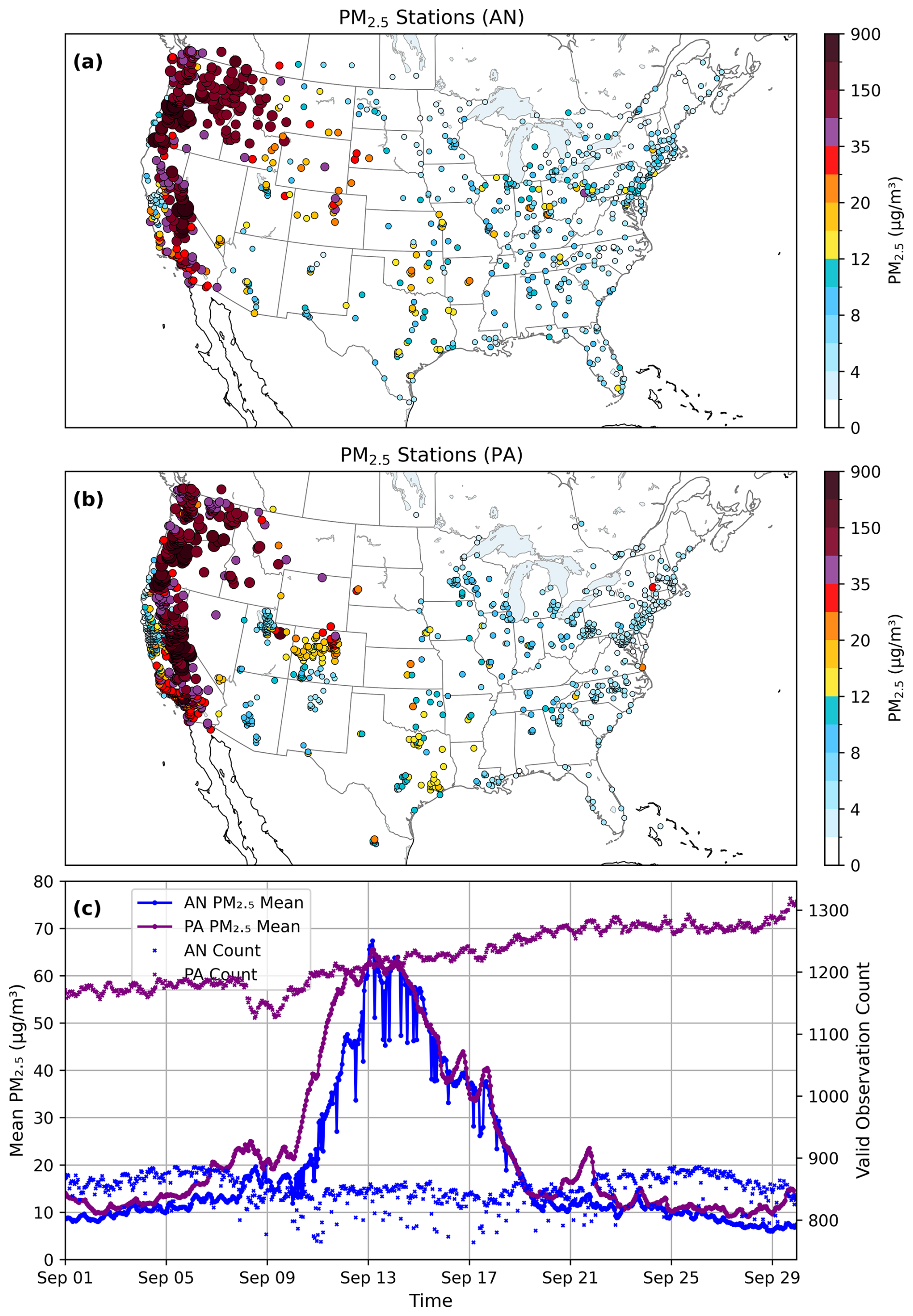
Figure 1 (a, b) Spatial distribution of AirNow(AN) and PurpleAir(PA) PM_2.5 monitoring stations on 12:00 UTC 16 September 2020. For PurpleAir, only stations that passed the quality control are shown. The displayed values are the corrected concentrations calculated using Eq. (6). (c) Time series of domain averaged PM_2.5 values and numbers from AirNow and PurpleAir observing networks.

3.3 Background error covariance

In this study, the background error standard deviation (Σ) for each control variable is constructed based on the background forecast; specifically, the error standard deviations of an aerosol variable are prescribed as proportional to its background values.

The proportional scaling factor s is approximately estimated by building a linear relationship between the PM_2.5 standard error (Σ) and the background forecast ${\mathrm{PM}}_{\mathrm{2.5}}^{\text{bkg}}$ concentrations:

$$\begin{array}{}\text{(7)}& \mathbf{\Sigma }=s\cdot {\mathrm{PM}}_{\mathrm{2.5}}^{\text{bkg}}\end{array}$$

The scaling factor s is subsequently applied to all PM_2.5 components, i.e., the 70 prognostic aerosol variables, to construct their error standard deviations.

This proportionality-based approach has also been adopted in the MOCAGE operational system (Colette et al., 2024), where background error standard deviations are similarly prescribed relative to background concentrations as a first-order approximation.

Tang et al. (2023) tested a similar method, in which the background PM_2.5 error variance is first estimated using the Hollingsworth–Lönnberg method (Hollingsworth and Lönnberg, 1986). A linear relationship is then established between the estimated PM_2.5 standard error and the background forecast ${\mathrm{PM}}_{\mathrm{2.5}}^{\text{bkg}}$.

Here we take the same idea but using an alternative approach to roughly estimate the background PM_2.5 forecast error variance. The background PM_2.5 error variance (Σ²) is estimated using PM_2.5 innovation information d defined in the Sect. 2.2, and observation error information R specified in the Sect. 3.2.3, specifically,

$$\begin{array}{}\text{(8)}& {\mathbf{\Sigma }}^{\mathrm{2}}=E\left(\mathit{d}{\mathit{d}}^{\mathrm{T}}\right)-\mathbf{R}\end{array}$$

In Eq. (8), E(⋅) denotes the mathematical expectation operator. The superscript T denotes the transpose of a vector. Equation (8) is valid under the assumption that observation and background errors are uncorrelated. This assumption is reasonable when the innovation vector d is calculated using forecasts from a free-running model without any aerosol data assimilation.

In this study, short-term (e.g., 3 h) PM_2.5 forecasts from a free run conducted during 1–21 September 2020 were used to compute the innovation vector d. This free run, referred to as the control run, is described in detail in the following section. Using the innovations and observation errors from Sects. 2.2 and 3.2.3 as inputs to Eq. (8), the background error variance of PM_2.5 was first estimated. This error, along with the background values, was then used in Eq. (7) to estimate the scaling factor, s. This scaling factor was subsequently applied in all assimilation experiments presented in this study.

This proportionality-based approach implicitly assumes that displacement errors and severe background underprediction errors do not dominate, thereby focusing the assimilation process on correcting amplitude. It offers several benefits:

• It helps constrain analysis increments to physically meaningful regions. For example, it prevents the generation of sea salt aerosol increments over inland areas where no sea salt is present in the background. This is a problem that can occur when using GSI's height-dependent or latitude–height-dependent background error variance formulations, particularly when individual aerosol species are used as control variables.

• It introduces location- and time-dependent background error variance information, improving the realism of background error specification. Moreover, the aerosol variables that dominate background errors vary by location and assimilation cycle, rather than being consistently dominated by the same species when using constant static background error statistics. For example, organic and black carbon typically exhibit the largest errors in wildfire regions and downwind areas affected by smoke, whereas other regions may be dominated by non-organic aerosols.

An example of domain averaged background PM_2.5 error standard deviation from a data assimilation run that assimilated both AirNow and PurpleAir PM_2.5 is shown in Fig. 2. This figure is intended to illustrate the main difference to static constant background errors, though the actual errors used in the data assimilation experiments are the errors of the individual aerosol control variables. It is obvious that this approach produces dynamically location- and time-dependent varying error estimates that yield particularly large error variances during the peak fire events from 10–20 September 2020.

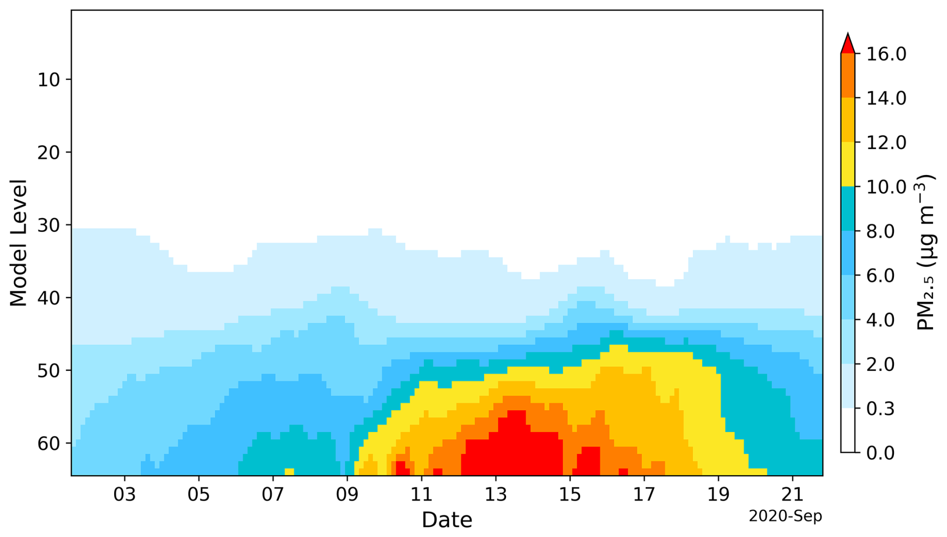
Figure 2 Domain averaged PM_2.5 error standard deviations for the data assimilation run that assimilated both AirNow and PurpleAir PM_2.5.

The background error correlation matrix C is modeled using a generic diffusion correlation operator designed for short length scales, as implemented in the System-Agnostic Background Error Representation (SABER) repository (Sluka, 2024). The primary input parameters are the horizontal and vertical cutoff length scales, defined as the distances beyond which correlations are zero. A horizontal cutoff scale of 100 km is applied, consistent with estimates derived from NMC statistics in previous GSI applications (Wang et al., 2021). For vertical correlations, this study uses a cutoff length scale of 12 model levels, which helps confine the influence of surface PM_2.5 observations within the average daytime planetary boundary layer (PBL) height (∼1450 m) and has demonstrated improved surface PM_2.5 prediction as will be discussed in Sect. 4.

3.4 Update of total particle number and surface area concentrations

After the aerosol mass concentration has been analyzed, total particle number concentration and total surface area concentration can be updated accordingly. For simplicity, it is assumed that the ratio of the particle number concentration to total particulate volume within each mode (I, J, K) remains the same as in the background. Total particulate volume is used instead of mass mixing ratio because it is proportional to the particle number concentration (see Eq. 3 in Binkowski and Roselle, 2003). A similar assumption was adopted by Li et al. (2013) to update number concentrations for the WRF-Chem model.

The number of particles is updated using the following relation:

$$\begin{array}{}\text{(9)}& N_{\mathrm{a}}={\displaystyle \frac{N_{\mathrm{b}}}{V_{\mathrm{b}}}}\times V_{\mathrm{a}}\end{array}$$

Where:

• N_a and N_b are the number of particles in the analysis and background, respectively, within each mode.

• V_a and V_b the total particulate volumes in the analysis and background, respectively, within the same mode.

The total particulate volume (V_a or V_b) within each mode is calculated by dividing the mass concentration of each aerosol variable by its corresponding density in that mode, and then summing the results. This updating approach implicitly assumes that changes in volume across the three modes are driven solely by variations in particle number, rather than shifts in the aerosol size distribution. The total particulate surface area within each mode is then updated using the same volume ratio, i.e., $\frac{V_{\mathrm{a}}}{V_{\mathrm{b}}}$ multiplied by the background surface area.

In preparatory work for this study, six-hourly cycling experiments (Wang et al., 2025a) have shown that updating these variables is crucial for improving AQMv7 performance. In contrast, previous work using GSI with earlier developmental versions of AQM did not update these variables, primarily because those model versions were less advanced than the current operational AQMv7. As a result, there was still significant room for improving prediction skills.

3.5 Experiments

In the operational AQMv7 configuration, aerosol initial conditions (IC) are warm-started from a previous forecast cycle. In contrast, in cycling data assimilation and forecasting experiments, the data assimilation system provides aerosol initial conditions for the subsequent forecast, while the short-term (3 h) forecast serves as the background for the next data assimilation cycle. A schematic of the data assimilation and forecasting cycles is shown in Fig. 3.

Figure 3 A schematic of the data assimilation and forecasting cycles.

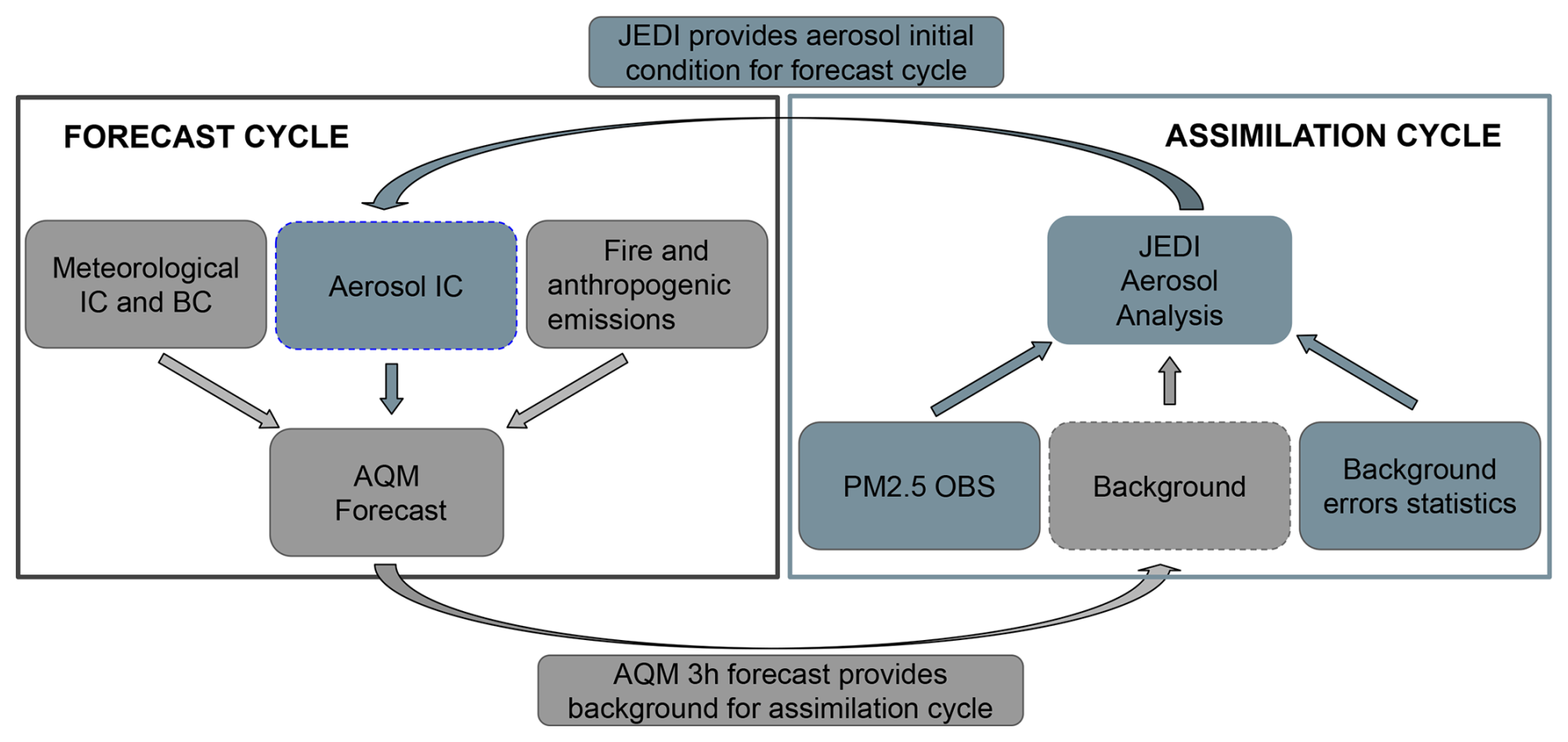
In the assimilation cycle, JEDI updates the aerosol analysis by combining PM_2.5 observations with the background information. The updated aerosol analysis, together with meteorological initial conditions, emissions, and other inputs, is then used to initialize the subsequent forecasts in the forecast cycle. Note that the meteorological initial conditions are not updated by JEDI but are generated from GFS forecast outputs of the previous GFS cycle.

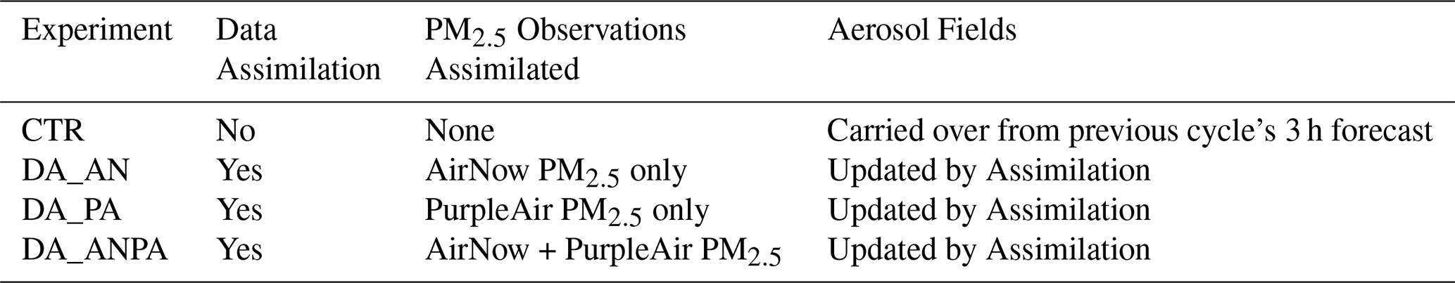
Four experiments were conducted to evaluate the performance of JEDI/AQM PM_2.5 DA. Table 1 provides a description of the experiments.The first experiment is a control run (CTR), in which meteorological initial and boundary conditions are updated every 3 h, while chemical and aerosol fields are carried over from the 3 h forecast of the previous cycle. The other three experiments incorporate data assimilation: DA_AN, DA_PA, and DA_ANPA, which assimilate AirNow PM_2.5 only, PurpleAir PM_2.5 only, and both AirNow and PurpleAir PM_2.5 observations, respectively.

Table 1 Descriptions of the experiments.

Like the CTR experiment, all DA experiments are conducted as 3-hourly cycling runs. Data assimilation is performed every 3 h, and a 3 h forecast is launched at each cycle. This 3 h forecast serves as the background for the subsequent data assimilation and forecasting cycle. In addition, forecasts initialized at 00:00, 06:00, 12:00, and 18:00 UTC are extended to 24 h for evaluation purposes. The experimental period spans from 12:00 UTC on 1 September to 18:00 UTC on 21 September 2020. It is noted that to reduce random sensor noise and improve comparability with the model resolution (∼13 km), the PurpleAir PM_2.5 data were spatially averaged onto a 0.1°×0.1° latitude–longitude grid before assimilation.

4 Results

This section provides an overview of the impact of DA on PM_2.5 forecasts. A total of 80 forecasts – initialized four times daily from 00:00 UTC on 2 September to 18:00 UTC on 21 September 2020 – are used to evaluate model performance. AirNow PM_2.5 observations are used to verify the forecast. Forecast errors are assessed using bias, mean absolute error (MAE), and root mean square error (RMSE). Forecast performance is evaluated using box plots, which illustrate the distribution, spread, and central tendency of forecast errors. Time series of PM_2.5 at various forecast hours are presented to examine the temporal evolution of forecast performance. Additionally, spatial distributions of PM_2.5 including observations, forecasts, forecast errors, and forecast differences are analyzed to evaluate the spatial impact of data assimilation on PM_2.5 predictions.

Figure 4 presents the bias, mean absolute error (MAE), and root mean square error (RMSE) for the 1–24 h forecast of domain-averaged PM_2.5. Domain averages are computed over all states in the mainland United States. From the bias statistics (Fig. 4a), it is seen that the bias in the control run follows an upward trend initially, then reverses into a downward trend. The data assimilation runs show a similar trend, as data assimilation primarily corrects the model state and does not fully resolve inherent model bias. The control run underpredicted surface PM_2.5 throughout the 24 h forecast period by about 1 µg m⁻³. This underprediction was improved in the data assimilation experiments. The two assimilated experiments, DA_AN and DA_ANPA, reduced the 1–24 h mean bias to −0.2 and −0.3 µg m⁻³, respectively. The PurpleAir PM_2.5 assimilation experiment (DA_PA) also slightly improved the 1–24 h mean bias.

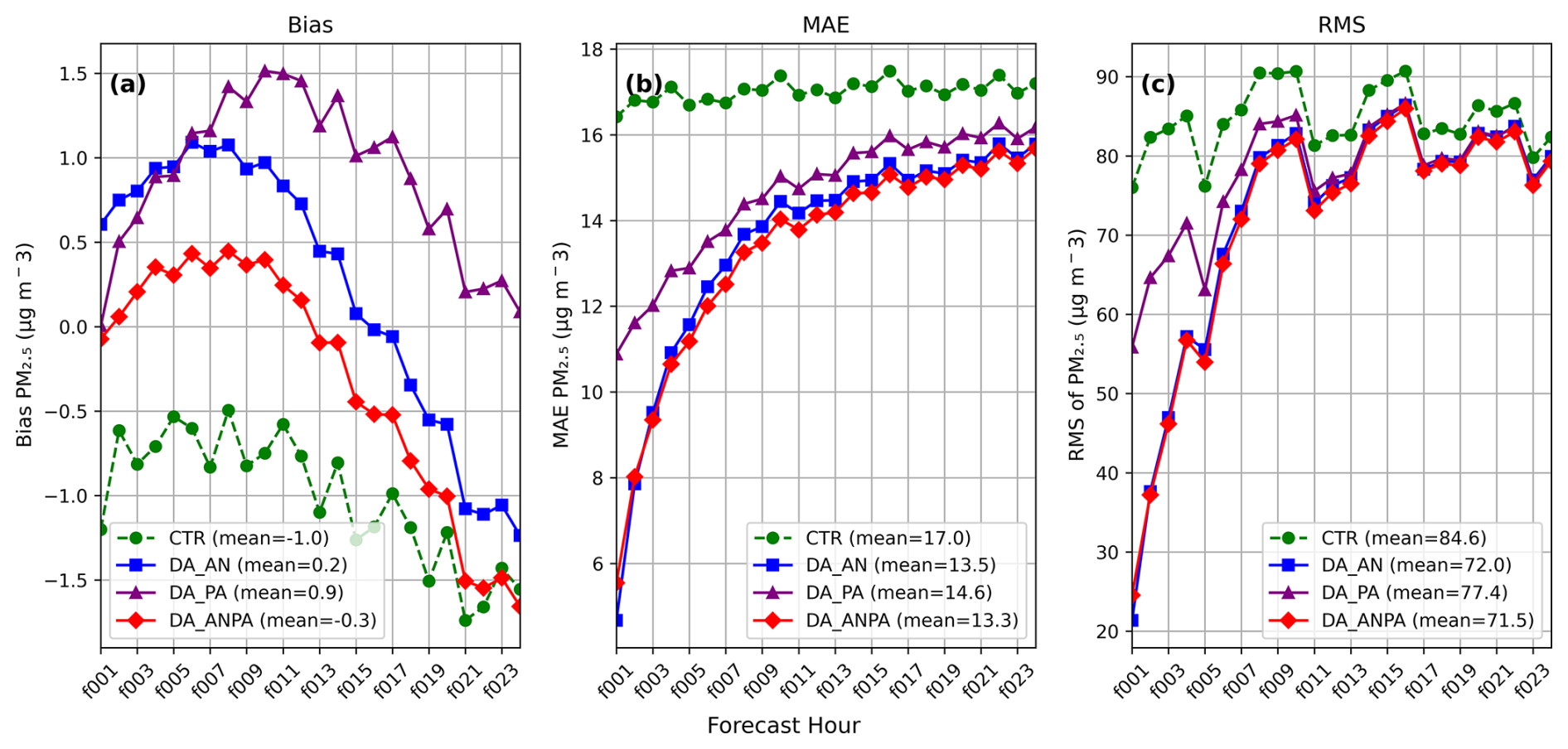
Figure 4 PM_2.5 forecast errors for 1–24 h lead times based on 80 forecasts initialized four times daily during 2–21 September 2020. Domain-averaged over CONUS. The x axis represents forecast lead times from 1 to 24 h. (a) Bias, (b) Mean Absolute Error (MAE), (c) Root Mean Square Error (RMSE).

It is seen that DA_PA produces a near zero bias at 1 h forecast, however this is due to large positive and negative biases canceling out. Therefore, it should be used together with norms like Mean Absolute Error (MAE) and Root Mean Square Error (RMSE), which quantify the actual magnitude of forecast errors.

In terms of MAE and RMSE, all the three data assimilation experiments reduced the surface PM_2.5 forecast error throughout the 24 h forecast period. The added value of assimilating PurpleAir PM_2.5 data alongside AirNow observations is evident in the consistent MAE reduction (Fig. 4b). Its impact on RMSE (Fig. 4c) is also positive, though relatively small. Overall, all the data assimilation experiments show improved forecast skill compared to the control run.

Figure 5 shows box-and-whisker plots of PM_2.5 forecast bias. Across all forecast hours, the interquartile range (IQR) – represented by the height of the boxes – is consistently smaller for the DA experiments compared to the control run. This indicates reduced forecast error spread between the 25th and 75th percentiles and suggests more consistent forecasts in the DA experiments. Although the median forecast bias in the control run is sometimes closer to zero, the DA_ANPA experiment performs comparably in terms of central tendency while showing clear improvements in reducing the mean forecast bias, as also reflected in Fig. 4a. Among the DA experiments, DA_AN and DA_ANPA show the most consistent improvement at 24 h lead times, with DA_ANPA slightly outperforming others during the early forecast hours (e.g., hour 1 to 12). This suggests that assimilating PurpleAir observations in addition to AirNow helps reduce bias and brings the forecasts closer to observed PM_2.5 values in the short term.

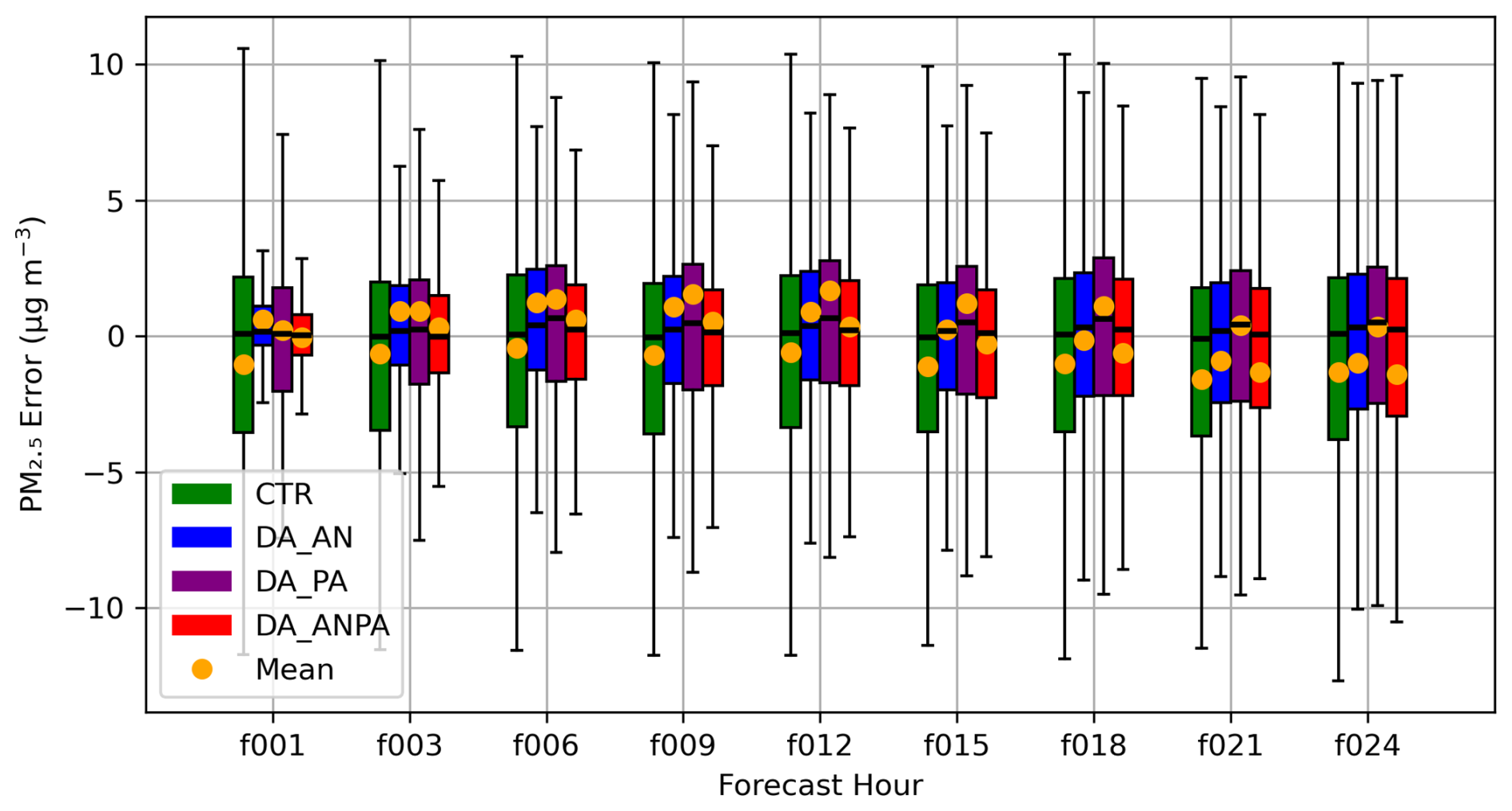
Figure 5 Box-and-whisker plot of PM_2.5 forecast bias. Orange dot: domain averaged mean; Bottom edge  =  Q1 (25th percentile); Top edge  = Q3 (75th percentile); Height  =  Interquartile Range (IQR = Q3 − Q1); Horizontal line inside box: The median (50th percentile); Whiskers: Extend to the min and max values within 1.5× IQR from Q1 and Q3.

Figure 6 shows time series of PM_2.5 averaged over CONUS at forecast hours 1, 12, and 24, respectively. Consistent with the evaluations in Figs. 4 and 5, all DA experiments generally improve PM_2.5 forecasts. Notably, all DA experiments help correct underpredictions during 2–9 and 14–17 September. In addition, the substantial overprediction during 9–13 September observed in the control run is partially mitigated by the DA experiments. Among the DA experiments, DA_AN and DA_ANPA show comparable performance and both outperform DA_PA.

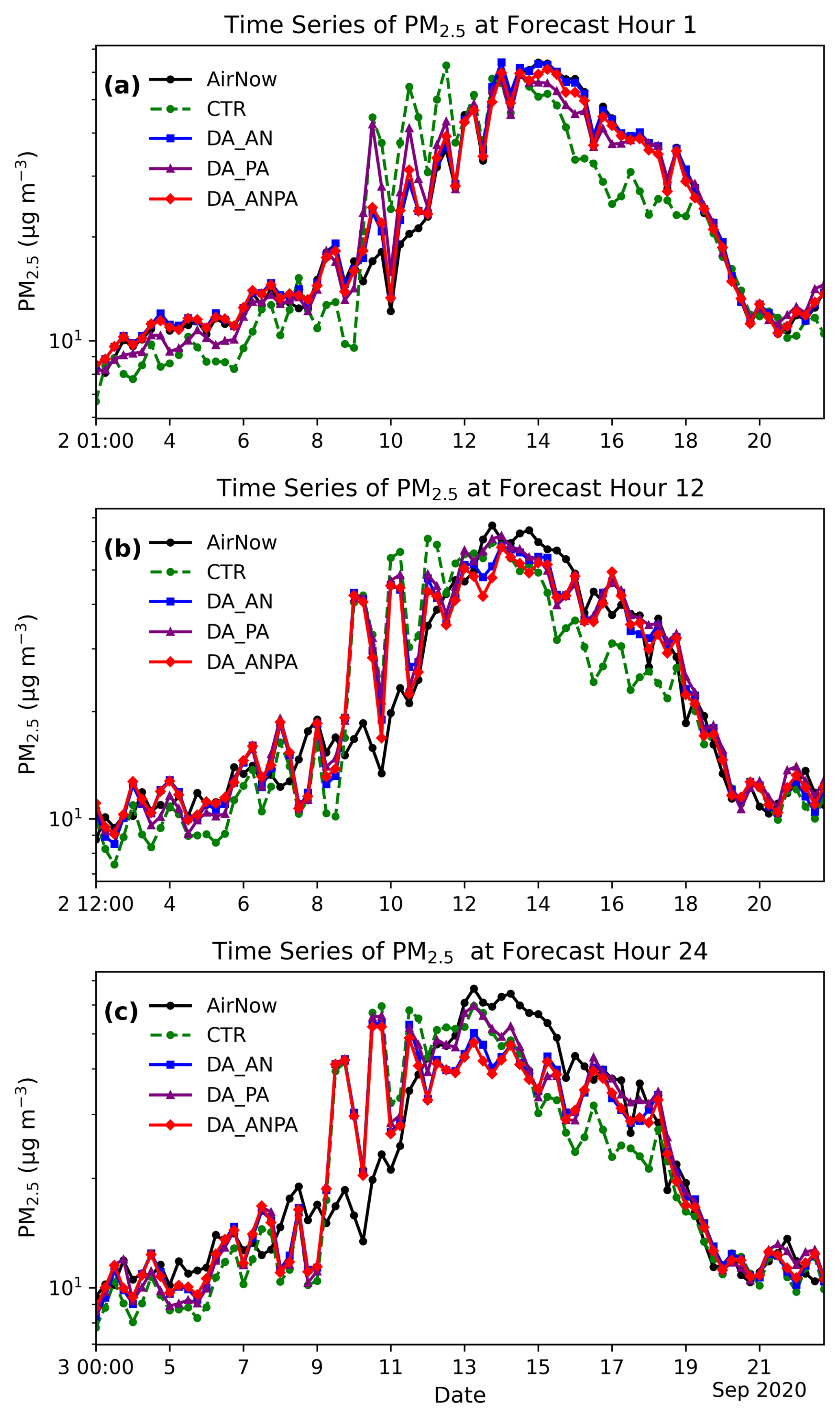
Figure 6 Time series of PM_2.5 averaged over CONUS for (a) forecast hour 1, (b) forecast hour 12, and (c) forecast hour 24. The y axis is shown on a logarithmic scale.

While we have investigated the impact of DA on PM_2.5 forecasts in terms of temporal evolution, it is also important to examine the spatial distribution of forecast fields, associated errors, and the impact of PM_2.5 data assimilation.

Figure 7 presents the spatial distribution of temporally averaged PM_2.5 forecasts at forecast hour 1, based on 80 forecasts initialized four times daily (00:00, 06:00, 12:00, and 18:00 UTC) from 2–21 September. The effects of wildfire events are clearly seen in Fig. 7a, c and e across California, Oregon, and Washington – where the fires occurred – as well as in downstream regions such as Montana, Wyoming, Utah, and Colorado impacted by smoke advection and transport.

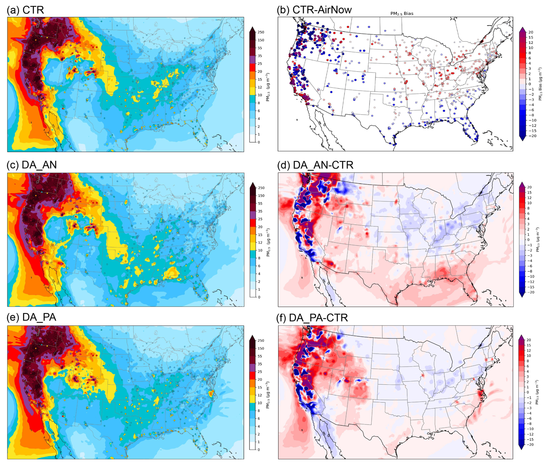
Figure 7 Spatial distribution of average PM_2.5 at forecast hour 1, based on 80 forecasts initialized four times daily (00:00, 06:00, 12:00, and 18:00 UTC) during 2–21 September. (a) PM_2.5 in experiment CTR (shaded) overlaid with AirNow PM_2.5 observations (filled dots). (b) PM_2.5 bias in experiment CTR. (c) PM_2.5 in experiment DA_AN (shaded) overlaid with AirNow PM_2.5 observations. (d) PM_2.5 difference between experiments DA_AN and CTR. (e) PM_2.5 in experiment DA_PA (shaded) overlaid with AirNow PM_2.5 observations. (f) PM_2.5 difference between experiments DA_PA and CTR.

1 h PM_2.5 forecast errors in the control run are evident in Fig. 6a but are more clearly highlighted in Fig. 7b, which shows the difference between the control run and AirNow observations. Significant overpredictions appear along the California coast, as well as in parts of the Midwest and Northeast US, including Tennessee, Kentucky, West Virginia, and Virginia. Conversely, notable underpredictions are found over Colorado, New Mexico, much of Texas and Oklahoma, and several Gulf Coast states.

Both DA_AN (Fig. 7c and d) and DA_PA (Fig. 7e and f) show similar spatial correction patterns across California, Oregon, and Washington, particularly in reducing overpredictions along the California coast. They also produce comparable large-scale adjustments across the Northeast, Midwest, and Southern US, with their spatial patterns (Fig. 7d and f) largely opposite in sign to those in the CTR–AirNow difference (Fig. 7b). This indicates that both DA experiments effectively mitigate the control run's over- and underpredictions.

However, the magnitude of the corrections is generally smaller in DA_PA than in DA_AN. DA_PA shows its strongest impact over Nevada, northern Utah, Colorado, and southwestern New Mexico, where it helps alleviate regional underpredictions (Fig. 7e and f). These improvements are also observed in DA_ANPA, whose spatial pattern closely resembles DA_AN except over these few states (figures not shown).

The above analysis shows that data assimilation effectively corrects the 1 h forecast errors in the control run, particularly in the DA_AN and DA_ANPA experiments. It is therefore of interest to examine how data assimilation affects longer forecast lead times. Figure 8 presents the MAE from the CTR experiment and the percentage change in MAE (%) between the data assimilation (DA) experiments and the CTR experiment at the 24 h forecast lead time. Negative values in Fig. 8b–d indicate a reduction in MAE.

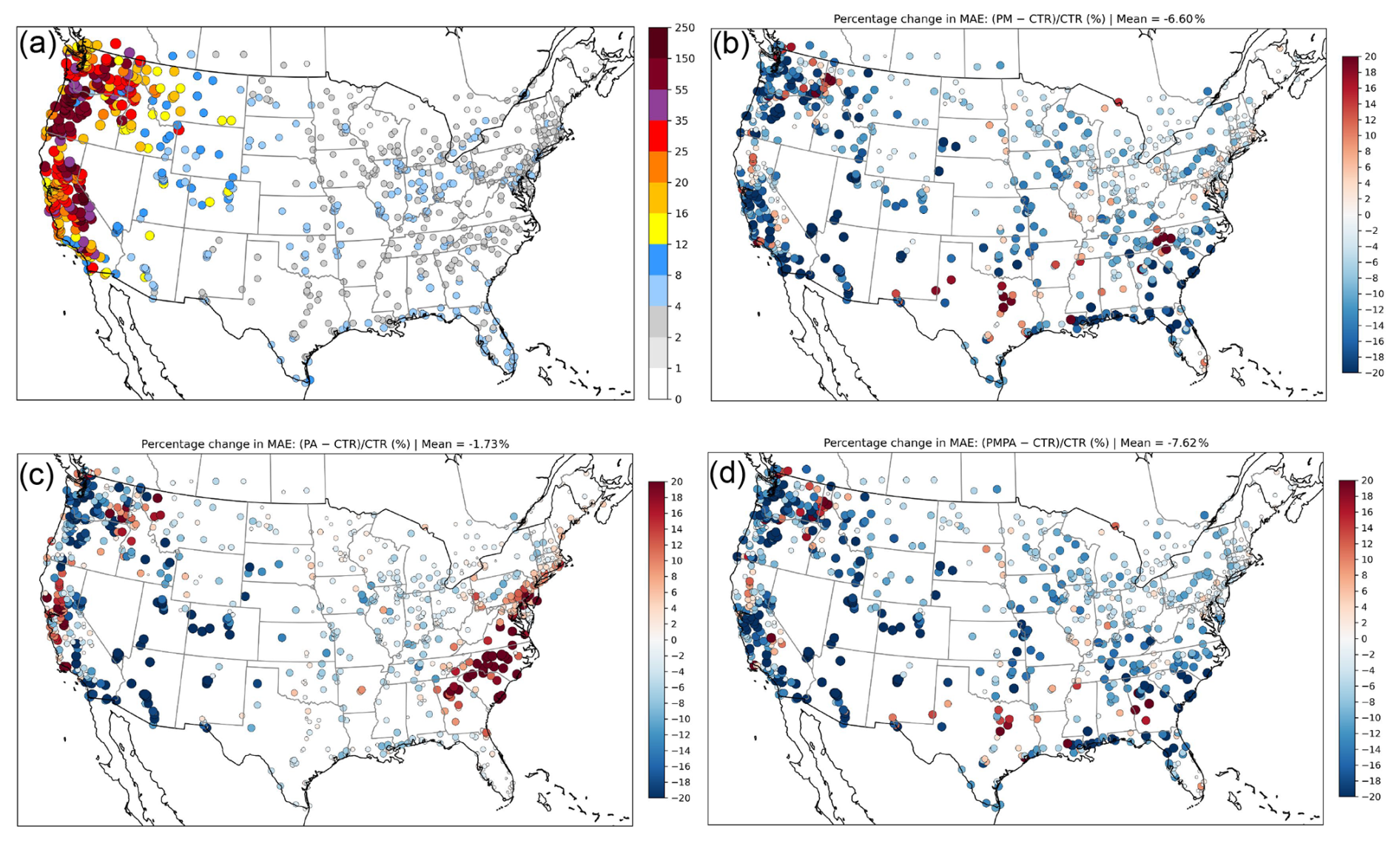
Figure 8 (a) MAE from the control (CTR) experiment. Percentage change in MAE (%) relative to CTR for (b) DA_AN, (c) DA_PA, and (d) DA_ANPA. The percentage change is calculated as (MAE(DA) − MAE(CTR)) $/$ MAE(CTR) ×100.

It is seen from Fig. 8a that the largest MAE values occur in California, Oregon, Washington, Idaho, Montana, Wyoming, Utah, Colorado, and Arizona. The PM_2.5 MAE in these states is generally greater than 10 µg m⁻³, with maximum values exceeding 150 µg m⁻³ at certain stations in California, Oregon, and Washington. In contrast, regions less affected by wildfire smoke exhibit MAE values below 10 µg m⁻³.

All DA experiments (Fig. 8b–d) show overall reductions in MAE at most stations. MAE reduction varies by location, with substantial improvements observed in regions with large forecast errors, such as California, Oregon, Washington, and Idaho, where MAE is reduced by approximately 20 %. On average, assimilation of AirNow PM_2.5 observations alone significantly improves the 24 h forecast skill, with MAE reductions of 6.6 % based on MAE percentage changes averaged over all stations. In contrast, assimilation of PurpleAir data alone reduces the MAE by only 1.7 %. Assimilating both AirNow and PurpleAir PM_2.5 observations reduces the MAE by 7.6 %, indicating that PurpleAir data provides complementary value to AirNow in improving forecast skill.

In the DA_PA experiment, a few eastern coastal states from Georgia to Virginia exhibit large percentage increases in MAE. These increases are associated with relatively small absolute errors, as MAE values in the CTR experiment over these states are typically only 2–4 µg m⁻³ (Fig. 8a). Increased MAE is also present at several stations at the 1 h forecast lead time in the DA_PA experiment in these areas (figure not shown). In contrast, the MAE increase at the 24 h forecast lead time is much less pronounced in the experiment assimilating only AirNow PM_2.5 observations. This behavior suggests potential quality issues in the assimilated PurpleAir data in those areas that require further investigation, although a contribution from model errors cannot be ruled out.

To further examine model performance across different regions, error statistics (bias, MAE, and RMSE) for the averaged 1–24 h PM_2.5 forecasts from the control and data assimilation experiments over the 10 EPA regions are analyzed. Figure 9 presents the EPA Regions 1–10 and Averaged 1–24 h PM_2.5 forecasts errors statistics in each EPA region.

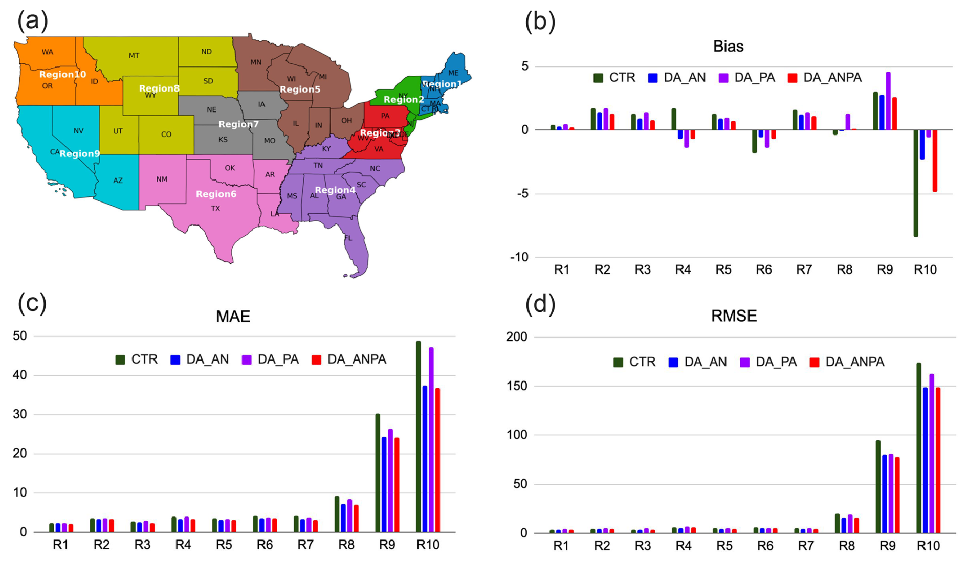
Figure 9 (a) EPA Regions 1–10. Averaged 1–24 h PM_2.5 forecasts errors: (b) Bias, (c) MAE and (d) RMSE.

In terms of bias (Fig. 9b), the DA_AN and DA_ANPA forecasts show improved performance relative to the control run. The DA_PA experiment also improves bias over most EPA regions, except for increased overprediction in EPA regions 8 and 9. For MAE and RMSE, the DA_AN and DA_ANPA experiments generally show improved performance across all EPA regions. The DA_PA experiment also exhibits improved, or at least comparable, MAE relative to the control run. However, DA_PA shows slightly increased RMSE over EPA regions 1–4, while reduced RMSE is found over other EPA regions.

Substantial reductions in MAE and RMSE are observed over EPA regions 8–10, where fire events occurred and/or where regions were most influenced by transported smoke. This is consistent with the large 1 h MAE reduction shown in Fig. 8. Notably, the DA_PA experiment, which assimilates PA observations alone, reduces both MAE and RMSE over EPA regions 8–10. Assimilating PurpleAir data together with AirNow data results in slightly smaller MAE and RMSE over these regions, suggesting that PurpleAir observations nonetheless provide complementary information to AirNow in these regions.

5 Summary and discussion

The latest version of NOAA's regional AQM system became operational on 14 May 2024. This system is based on the online coupling of the FV3 atmospheric model with the CMAQ model within the UFS framework. To improve initial conditions for AQM and enhance predictions of wildfire impacts on air quality, the capability to assimilate PM_2.5 observations into AQMv7 was developed within JEDI and evaluated using its 3D-Var assimilation component in this study. The developed assimilation scheme can also be used to generate analysis (reanalysis) dataset for other applications, for example, providing data for training artificial intelligent models used in air quality prediction.

Data assimilation experiments were conducted for the September 2020 Western US wildfire episode, using 3-hourly cycling with observations from the AirNow and PurpleAir networks. In the data assimilation experiments, the location- and time-dependent background error standard deviations of an aerosol variable are specified as proportional to its background values, using a diagnosed scaling factor. In addition to updating the analyzed aerosol variables in each mode, the particle number concentration and surface area of each mode are also updated. The results show that assimilating AirNow PM_2.5 observations improves 1–24 h forecast skill. Assimilating PurpleAir data alone yields modest improvements in MAE. Combining PurpleAir with AirNow observations provides additional benefit by slightly further reducing MAE relative to AirNow-only assimilation, indicating that PurpleAir observations nonetheless provide complementary information to AirNow. The AirNow data assimilation alone or with PurpleAir data generally show reduced MAE and RMSE across all EPA regions, whereas the largest reductions in MAE and RMSE are observed over regions affected by fire events and/or strongly influenced by transported smoke. The positive impact of PurpleAir data assimilation on smoke prediction during the September 2020 wildfires has also been demonstrated in an experimental Rapid Refresh Forecast System coupled with the Smoke and Dust Model (Wang et al., 2023), where it significantly reduced the model's 24 h underprediction of surface PM_2.5. Given that PurpleAir data coverage has improved since September 2020, the results of this study further highlight its potential to complement AirNow observations by filling spatial gaps and improving PM_2.5 analysis and forecast skill.

In this initial development and evaluation of aerosol data assimilation in JEDI for AQMv7, the control variables are defined as individual forecast aerosol variables. In previous work on aerosol data assimilation for an earlier version of AQM using the GSI system (Wang et al., 2021), one option for the control variables was to define them as the total aerosol mass in each of the three modes, resulting in just three control variables. A control variable transform was then applied to partition the analysis increments across these modes to individual aerosol species, based on the ratio of each species' mass to the total mass within the corresponding mode. The use of total aerosol mass in the three modes as control variables – thereby reducing the number of control variables from 70 to 3 – is planned for a future phase of development. The use of total masses as control variables also reduces the cost of the background error statistics calculation and iterative minimization (Kumar et al., 2019).

This study focused on surface-level PM_2.5 and did not incorporate vertical profile constraints with satellite-based aerosol optical depth (AOD) retrievals, which could further enhance forecast skill. A key challenge is the need for a robust forward operator in the CRTM AOD module – specifically, the creation and validation of lookup tables (LUTs) for AOD calculations with AQM. As an intermediate solution, existing LUTs in CRTM, such as the GEOS-5 LUTs, have been tested by grouping and mapping AQM aerosol species to those used in GEOS-5 (Wang et al., 2025). AOD assimilation also depends on an accurate vertical distribution of aerosols in the background field so that the CRTM AOD operator can provide meaningful gradient information at the correct vertical levels to constrain the analysis update. However, AQM models have shown deficiencies for the September 2020 fire events in representing smoke concentrations at and above plume rise levels, largely due to how fire emissions are injected into the model. This will be improved in the next update of the operational AQM.