EcoTWIN 1.0: a fully distributed tracer-aided ecohydrological model tracking water, isotopes, and nutrients

The value of stable water isotopes in constraining process representation in hydrological models is well acknowledged with numerous tracer-aided hydrological models developed in recent years, yet few have leveraged these benefits for more robust water quality modelling. Therefore, we introduce EcoTWIN, a fully distributed tracer-aided ecohydrological model that simultaneously tracks water, isotope, and nutrient fluxes. A thorough model test was conducted by calibrating EcoTWIN against discharge, in-stream isotopes, and NO₃–N concentrations (1980–2024) in 17 large-scale (10³–10⁵ km²) European catchments spanning a wide range of geographic and climatic gradients. Furthermore, three reanalysis products (ERA5 snow depth, MODIS evapotranspiration, and GRACE surface water anomaly) were employed to further validate the capacity of EcoTWIN to reproduce associated but uncalibrated internal water fluxes. Results showed good model performance of both calibrated in-stream targets and uncalibrated internal fluxes in most catchments. Therefore, we conclude that EcoTWIN is a flexible, transferable modelling tool for prediction and process inference in terrestrial ecosystems ranging from boreal to subtropic climates. Constrained by tracer simulations, the model not only captures the celerity, but also the velocity of hydrological fluxes, thus providing spatio-temporally-explicit estimations of water ages and travel times. Such information provides opportunities to bridge catchment hydrology and water quality by linking travel times with biogeochemical processing kinetics. We demonstrate this with a proof of concept using Damköhler Number in nitrogen modelling.

1 Introduction

The development of ecohydrological models has been accelerating in the recent decades towards frameworks that are more spatially distributed (instead of lumped or semi-distributed) and complex (integrating more ecohydrological processes) (Pechlivanidis et al., 2011; Wellen et al., 2015). A few examples include SWAT (Arnold et al., 2012), HYPE (Lindström et al., 2010), and mHM-Nitrate (Yang et al., 2018), which have been widely applied worldwide. As process-based models, they are used not only as prediction tools for specific variables, but also as learning tools for model inference, i.e., to track the internal states/fluxes from available observations (Wang et al., 2024). This, however, poses challenges due to the considerable uncertainties in model inference.

Inference of internal processes is naturally uncertain due to the lack of direct observations, though such uncertainty can be constrained to some extent by rigorous split-sample calibration and validation. The reason we use “to some extent” here is based on the fact that most models are calibrated to a minimal number of variables, and 81 % of calibrations used data from a single gauge (mostly at a catchment outlet) as reviewed in Wellen et al. (2015). Additionally, from a technical perspective, “equifinality” further adds to the inference uncertainty due to the potential misinformation in data (uncertainty in model forcing and observations) and model structure (the use of simplified, abstract mathematics to simulate real world processes) (Beven, 2006). This can result in inaccurate process representations yielding deceptively good results through error compensation, thus leading to overconfidence in a model's ability to reproduce within-basin dynamics (Wen et al., 2024; Wu et al., 2025a). As acknowledged by the hydrological community, models calibrated solely against discharge at the catchment outlet reflect only the celerity of hydrological systems (pressure wave propagation), yet constituent transport in water quality modelling relies on the velocity (mass flux of the water) (McDonnell and Beven, 2014). Failure to reconcile these differences can lead to questionable process inferences from many ecohydrological and water quality models.

One way to strengthen model inference is to include auxiliary data for calibration (Efstratiadis and Koutsoyiannis, 2010). However, there is a paradox in multi-criteria calibration, as on the one hand, more auxiliary data will feed unique information to the calibration process, thus effectively constraining the model behaviour from an ecohydrological perspective; yet on the other hand, it increases the dimensionality of calibration thus resulting in degraded performance or failure of calibration from a technical perspective. The “curse” of dimensionality in ecohydrological modelling is universal for all the commonly used algorithms under both Bayesian and Pareto theories as demonstrated in Wu et al. (2025c). Therefore, modellers should expect the selected auxiliary data to contain as much information as possible (Nearing et al., 2020). For distributed modelling, the auxiliary data should reflect the cumulative contribution of all upstream reaches/regions, rather than variables that are highly dependent on local condition/processes (e.g. point-scale soil moisture and evapotranspiration measurements etc.).

Stable water isotopes, in this context, have powerful potential in cumulative flux tracking. As conservative tracers, ²H and ¹⁸O are independent of biogeochemical reactions and naturally integrate landscape heterogeneity, thus providing effective constraints on spatially distributed (dis)connections of hydrological flow paths as well as velocity of the hydrological systems which reflect flux-storage interactions (Jung et al., 2025; Tetzlaff et al., 2015). The value of tracers has long been recognised by hydrologists (Hooper et al., 1988), with many tracer-aided hydrological models developed and evolved in recent years from lumped (Birkel et al., 2011; Godsey et al., 2010), to semi-distributed (van Huijgevoort et al., 2016; Nan et al., 2021), and distributed structure (Kuppel et al., 2018; Remondi et al., 2018). However, few attempts have been made to integrate a tracer-aided hydrological structure into water quality modelling (Birkel and Soulsby, 2015; Jung et al., 2025), despite the need being evident for nearly four decades (Neal et al., 1988). Moreover, existing pioneering models are mostly conceptualised/lumped (Benettin et al., 2015; Dick et al., 2015) and/or loosely coupled via external tracer/water quality modules (Pesántez et al., 2023; Yang et al., 2024; Zhang et al., 2020). The external coupling of model chains transfer necessary internal states and fluxes between sub-models (e.g. hydrological fluxes for constituent mixing in water quality or isotopic modules) via online in-memory coupling (instead of offline on-disk coupling), thus significantly increasing the resources consumption in input/output operations. Such model chains, though providing useful scientific insights, can become problematic for large-scale applications owing to the exponential growth in computational and storage requirements. Therefore, there remains a need to develop a fully distributed, computationally efficient ecohydrological model that combines hydrological, isotopic, and water quality simulations.

This research gap motivated the development of EcoTWIN, the model that we present in this paper. To our knowledge, the model is one of the first distributed tracer-aided ecohydrological models that tracks water, isotopic, and nutrient fluxes simultaneously in a C$++$-based framework. For a thorough testing of EcoTWIN, 17 large European catchments were selected for calibration against discharge, in-stream isotopes, and NO₃–N concentrations. These catchments span over a wide range of geographic (Alpine to lowland plain) and climatic (from snow-dominated to Mediterranean) gradients. In addition, the robustness of modelled inference on uncalibrated internal fluxes were also compared with three remote sensing products (snow depth, evapotranspiration, and water storage). Given the overall good integrated performance in most catchments, EcoTWIN is presented as an ecohydrological modelling framework applicable for terrestrial ecosystems ranging from boreal to temperate and subtropical climates across a wide range of geographical environments. The subsequent sections are organised as follows: Sects. 2 and 3 introduce the model structure of EcoTWIN and details in calibration and validation; the model performance is shown in Sect. 4; in Sect. 5 we show the advantages of a tracer-aided ecohydrological framework with an example of how water ages bridge catchment hydrology and water quality models; finally, the current limitations and planned future development of EcoTWIN are also discussed.

2 Model description

EcoTWIN is fully distributed ecohydrological model implemented in C$++$. The model consists of hydrological, isotopic, and nitrogen modules, which simulate major ecohydrological states and fluxes from canopy to groundwater (Fig. 1). Aided by tracer simulations, the model is additionally able to track the water movement vertically and laterally via the calculation of water ages and travel times. For detailed information of model parameters please refer to Table S1.

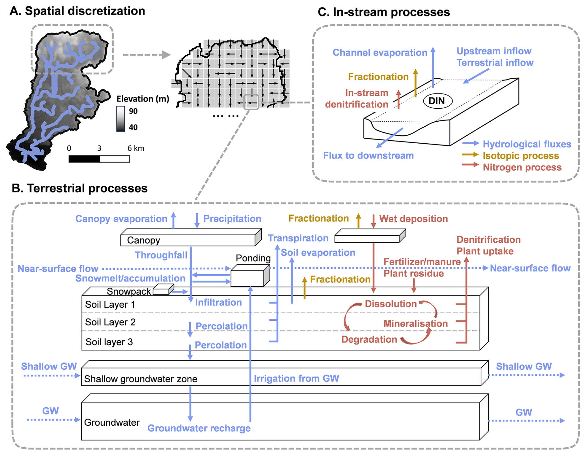
Figure 1 Model structure of EcoTWIN. As a distributed model, EcoTWIN disentangles the spatial domain into grid cells (A). In each grid cell, hydrological, isotopic, and nitrogen processes were simulated in canopy, snow, soils, shallow groundwater, and groundwater (B) and river channel if channels are present (C).

2.1 Hydrological module

EcoTWIN follows a typical multi-layer, top-down, bucket-type approach that resolves the water balance sequentially for the vegetation canopy, three soil layers, unsaturated zone, and groundwater. As the foundation of solute transport, the hydrological module employs a selective disassembly structure with multiple alternative conceptualisations possible for specific important hydrological processes. The configuration can be specified a priori based on the goal of modelling and prior knowledge of the studied catchment(s).

2.1.1 Soil properties

Before iterative simulations, soil characteristics are estimated using appropriate pedotransfer functions. Three different alternatives are provided, each of which requires different levels of inputs but all were found to provide robust estimation of soil porosity (θ_s), field capacity (θ_fc), wilting point (θ_wp), and hydraulic conductivity (Ks). All the soil properties are required for each soil layer/depth. This can be achieved via three alternative options: (i) assigning identical properties across the whole soil column, (ii) calculating separately for each depth based on depth-dependent inputs, or (iii) extrapolating deeper profile characteristics from the top soil properties based on a depth-dependent equation in Maneta and Silverman (2013).

The distribution of soil types and land use is assigned from raster file in EcoTWIN. This can be specified as a static boundary condition; alternatively, the distributions can also be updated dynamically via a user-specified interval to reflect any temporal changes due to land management.

2.1.2 Vertical fluxes

The vertical fluxes are resolved for storages in the canopy, soil layers, unsaturated zone, and groundwater. The mass balance of canopy storage (ΔC) follows:

$$\begin{array}{}\text{(1)}& \mathrm{\Delta }C=P-I-\mathrm{Th}\end{array}$$

where P, I, Th are precipitation, interception, and throughfall, respectively. The throughfall is calculated as the exceedance of current canopy storage from the maximum storage calculated by Leaf Area index LAI and a correlation parameter α.

$$\begin{array}{}\text{(2a)}& C_{\max }=\mathit{\alpha }\cdot \mathrm{LAI}\end{array}$$

Alternatively, the maximum canopy storage can be estimated with explicit consideration of precipitation intensity (Landgraf et al., 2023):

$$\begin{array}{}\text{(2b)}& C_{\max }=\mathit{\alpha }\cdot \mathrm{LAI}\cdot \left(\mathrm{1}-{\displaystyle \frac{\mathrm{1}}{\mathrm{1}+\mathrm{SCF}\cdot P/(\mathit{\alpha }\cdot \mathrm{LAI})}}\right)\end{array}$$

where SCF is the vegetation cover fraction calculated by LAI and an extinction coefficient (rE) adopted from HYDRUS-1D (Šimùnek et al., 2013):

$$\begin{array}{}\text{(3)}& \mathrm{SFC}=\mathrm{1}-\exp (\mathrm{rE}\cdot \mathrm{LAI})\end{array}$$

Then throughfall is calculated as the exceedance of canopy storage from the maximum:

$$\begin{array}{}\text{(4)}& \mathrm{Th}=\left(P+C\right)-C_{\max }\text{if}\left(P+C\right)>C_{\max }\text{else}\mathrm{0}\end{array}$$

After reaching land surface, throughfall becomes ponding water (S_Pond) or snow (S_snow) depending on a temperature threshold for separation (Thre_SN). Snow will melt and recharge the ponding water in warm conditions (air temperature Ta exceed Thre_SN) following a degree-day model.

$$\begin{array}{}\text{(5)}& \begin{array}{rl}\mathrm{melt}& =S_{\mathrm{snow}}\cdot min({\mathrm{dd}}_{\min }+{\mathrm{dd}}_{\mathrm{inc}}\cdot \mathrm{Th}\\ & \cdot \left(\mathrm{Ta}-{\mathrm{Thre}}_{\mathrm{SN}}\right),{\mathrm{dd}}_{\max })\end{array}\end{array}$$

Where dd_min and dd_max are the minimum and maximum of degree day factor, while dd_inc denotes the rate of increase in the degree-day factor per degree Celsius rise in temperature.

The available ponding water infiltrates into the top soil layer using Green-Ampt model (Kale and Sahoo, 2011; Maneta and Silverman, 2013), with infiltration capacity first calculated as a function of average soil moisture over the hydrologically active depth:

$$\begin{array}{}\text{(6)}& I_f=\mathrm{Ks}\cdot (\mathrm{1}+{\displaystyle \frac{\mathit{\psi }\cdot {\mathit{\theta }}_{\mathrm{s}}\cdot (\mathrm{1}-({\mathit{\theta }}_{\mathrm{1}}-{\mathit{\theta }}_{\mathrm{wt}})/({\mathit{\theta }}_{\mathrm{s}}-{\mathit{\theta }}_{\mathrm{wt}}\left)\right)}{{\mathit{\theta }}_{\mathrm{1}}\cdot d_{\mathrm{1}}}})\end{array}$$

Where θ₁, θ_s, θ_wt, and d₁ are the moisture content, porosity, wilting point, and depth in top soil layer; ψ is a parameter representing soil air entry pressure in m. Then potential infiltration (F_p) is determined from the lesser between the available ponding water (S_pd) and potential infiltration rate integrated over time before ponding occurs (I_f⋅t_p).

The actual infiltration (F) is solved iteratively using the Newton–Raphson scheme:

$$\begin{array}{}\text{(7)}& \begin{array}{rl}F=\mathrm{\Delta }\mathit{\theta }\cdot d_{\mathrm{1}}& =F_{\mathrm{p}}+\mathrm{Ks}\cdot w_{\mathrm{Ks}}\cdot \left(\mathrm{\Delta }t-t_{\mathrm{p}}\right)-\mathit{\psi }\mathrm{\Delta }\mathit{\theta }\\ & \cdot \ln \left({\displaystyle \frac{\mathit{\psi }\mathrm{\Delta }\mathit{\theta }+\mathrm{\Delta }\mathit{\theta }{d}_{\mathrm{1}}}{\mathit{\psi }\mathrm{\Delta }\mathit{\theta }+F_{\mathrm{p}}}}\right)\end{array}\end{array}$$

where w_Ks is anisotropy ratio of vertical to horizontal Ks.

The soil storage in each layer is conceptualised as two water pools – a gravitational, free-flowing pool and a capillary, soil-bound pool. The two pools are separated based on field capacity (Maneta and Silverman, 2013), and percolation happens when soil storage exceeds the threshold. Three alternative schemes are included in EcoTWIN.

In the first scheme, all water in excess of field capacity percolates to deeper layer:

$$\begin{array}{}\text{(8a)}& {\mathrm{Pc}}_i=\left({\mathit{\theta }}_i-{\mathit{\theta }}_{\mathrm{fc}}\right)\cdot d_i\end{array}$$

where Pc_i, θ_i and d_i depict the percolation, moisture content and depth from/in ith soil layer in m.

The second scheme additionally considers the hydraulic conductivity (Ks) following the conceptualisation in SWAT (Arnold et al., 2012):

$$\begin{array}{}\text{(8b)}& {\mathrm{Pc}}_i=\left({\mathit{\theta }}_i-{\mathit{\theta }}_{\mathrm{fc},i}\right)\cdot d_i\cdot \left(\mathrm{1}-\exp \left({\displaystyle \frac{-\mathrm{\Delta }t\cdot \mathrm{Ks}}{{\mathit{\theta }}_{\mathrm{s},i}-{\mathit{\theta }}_{\mathrm{fc},i}}}\right)\right)\end{array}$$

The third scheme relates percolation to the extent of soil saturation with an exponential parameter β (Kumar et al., 2013; Samaniego et al., 2010):

$$\begin{array}{}\text{(8c)}& {\mathrm{Pc}}_i=\left({\mathit{\theta }}_i-{\mathit{\theta }}_{\mathrm{fc},i}\right)\cdot d_i\cdot (\mathrm{1}-\exp (\mathit{\beta }\cdot \log ({\mathit{\theta }}_i/{\mathit{\theta }}_{\mathrm{s},i})\left)\right))\end{array}$$

For evapotranspiration, soil evaporation and transpiration are estimated separately. The separation of PET is realised by surface cover fraction introduced above:

$$\begin{array}{}\text{(9)}& \mathrm{PT}=\mathrm{PET}\cdot \mathrm{SCF};\mathrm{PE}=\mathrm{PET}-\mathrm{PT}\end{array}$$

Soil evaporation is simulated in the top soil layer based on the soil saturation:

$$\begin{array}{}\text{(10)}& {\mathrm{Evap}}_{\mathrm{s}}=\mathrm{PE}\cdot min\left({\displaystyle \frac{{\mathit{\theta }}_{\mathrm{1}}}{{\mathit{\theta }}_{\mathrm{fc},\mathrm{1}}}},\mathrm{1}\right)\end{array}$$

Transpiration is simulated in all soil layers based on the fractions (f_root,i) of root density (D_root,i) in each layer partitioned by soil depth and a parameter (γ_root):

$$\begin{array}{}\text{(11)}& {\displaystyle }{\mathrm{Tr}}_i=\mathrm{PT}\cdot f_{\mathrm{root},i}\cdot {\displaystyle \frac{{\mathit{\theta }}_{\mathrm{1}}-{\mathit{\theta }}_{\mathrm{wp},\mathrm{1}}}{{\mathit{\theta }}_{\mathrm{fc},\mathrm{1}}-{\mathit{\theta }}_{\mathrm{wp},\mathrm{1}}}}\text{(12)}& {\displaystyle }{f}_{\mathrm{root},i}=D_{\mathrm{root},i}/\sum _{j=\mathrm{1}}^m{D}_{\mathrm{root},j}\text{(13)}& {\displaystyle }{D}_{\mathrm{root},i}=\left(\mathrm{1}-{\mathit{\gamma }}_{\mathrm{root}}^{\left({\sum }_{j=\mathrm{1}}^m{d}_j\right)}\right)-\left(\mathrm{1}-{\mathit{\gamma }}_{\mathrm{root}}^{\left({\sum }_{j=\mathrm{1}}^i{d}_j\right)}\right)\end{array}$$

Channel evaporation is also estimated using Penman equation, which relies on net radiation, wind speed, air pressure, and air temperature as inputs.

The last soil layer percolates to an unsaturated storage in unsaturated zone (S_unsat). The compartment stores the excess water from soil and percolates either downward to groundwater storage (S_GW) or laterally downstream. The percolation to groundwater Pc_GW is determined by a weighting parameter p_GW as a proportion of unsaturated storage:

$$\begin{array}{}\text{(14)}& P{c}_{\mathrm{GW}}=S_{\mathrm{unsat}}\cdot p_{\mathrm{GW}}\end{array}$$

Additionally, irrigation is conceptualised in EcoTWIN, which is realised via the water extraction from river or groundwater. The source is determined by the geographic location: for a grid cell with channel network, water is extracted directly from river, and local groundwater is used as irrigation source for non-channel grids. The amount of extraction is estimated from a predefine coefficient for crop water demands (w_irr) from which the deficit is calculated for each of the m soil layers.

$$\begin{array}{}\text{(15)}& \mathrm{deficit}=\sum _{i=\mathrm{1}}^m\left({\mathit{\theta }}_{\mathrm{fc},i}-{\mathit{\theta }}_{\mathrm{wp},i}\right)\cdot w_{\mathrm{irr}}\cdot d_i\end{array}$$

Note that the irrigation can switch to groundwater extraction if river storage cannot fill the deficit.

2.1.3 Lateral fluxes

In EcoTWIN, grid cells are connected laterally at three levels - surface, unsaturated zone, and groundwater. Note that some models omit the unsaturated storage and directly calculate excess water to drain based on the saturation extent of the bottom soil layer (e.g., EcH₂O-iso, Kuppel et al., 2018). EcoTWIN did not follow this conceptualisation because in reality, the lateral drainage is focused in the saturated zone, and thus the bottom of the soil layer instead of the whole soil profile. The drainage of an entire soil layer thus brings considerable uncertainty to the velocity of lateral transport when the lower boundary of the soil is a parameter to tune in calibration. For instance, a large soil depth will dramatically reduce the velocity of interflow drainage and slow down the mixing of constituents, though this might still perfectly reproduce the celerity (hydrograph) for purely hydrological modelling. Our conceptualisation (an independent unsaturated compartment) aligns with most hydrological models (Arnold et al., 2012; Yang et al., 2018) and fits the recent analysis supporting the dominant role of lateral drainage over vertical transports globally (McMillan et al., 2025).

By the end of each timestep, ponding water receives upstream inputs and contributes to channel storage if the grid is connected to the channel network, while non-channel grid has Ovf_C=0:

$$\begin{array}{}\text{(16)}& {\mathrm{Ovf}}_{\mathrm{C}}=({\mathrm{Ovf}}_{\mathrm{T},\mathrm{in}}+S_{\mathrm{pond}})\cdot p_{\mathrm{Ovf}}\cdot \mathrm{d}{x}_{\mathrm{C}}/\mathrm{d}{x}_{\mathrm{T}}\end{array}$$

dx_C and dx_T are the channel length and size of terrestrial grid cell; p_Ovf is a weighting parameter for channel recharge. Then the remaining ponding water routes to downslope terrestrial grid following the topographic gradient. In none-channel grid cells, all available ponding storage routes lateral downstream (Ovf_C=0):

$$\begin{array}{}\text{(17)}& {\mathrm{Ovf}}_{\mathrm{T},\mathrm{out}}=\left({\mathrm{Ovf}}_{\mathrm{T},\mathrm{in}}+S_{\mathrm{pond}}\right)-{\mathrm{Ovf}}_{\mathrm{C}}\end{array}$$

Similarly, unsaturated storage contributes first to channel storage in grid cells within channel network, while non-channel grid cells have Inf_C=0:

$$\begin{array}{}\text{(18)}& \begin{array}{rl}{\mathrm{Inf}}_{\mathrm{C}}& =\left({\mathrm{Inf}}_{\mathrm{T},\mathrm{in}}+S_{\mathrm{vadose}}\right)\cdot K_{\mathrm{vadose}}\\ & \cdot \left(\mathrm{1}-e^{-\mathrm{1}\cdot {\exp }_{\mathrm{Inf}}\cdot \left({\mathrm{Inf}}_{\mathrm{T},\mathrm{in}}+S_{\mathrm{vadose}}\right)}\right)\cdot p_{\mathrm{Inf}}\end{array}\end{array}$$

where K_vadose is the effective conductivity of lateral transport in the unsaturated zone; while exp_Inf is an exponential parameter determining the strength of positive correlation between recharge and current unsaturated storage. Then the remaining unsaturated storage is partially routed to downslope grid cell following a linear approximation of Kinematic wave equation, which assumes gravitational flux per unit width Inf_T,out is proportional to the subsurface hydraulic conductivity (K_vadose) and bedrock slope (slope approximated from the surface slope):

$$\begin{array}{}\text{(19)}& {\mathrm{Inf}}_{\mathrm{T},\mathrm{out}}=\left({\mathrm{Inf}}_{\mathrm{T},\mathrm{in}}+S_{\mathrm{unsat}}-{\mathrm{Inf}}_{\mathrm{C}}\right)\cdot \left(\mathrm{1}+\mathit{\alpha }\cdot {\displaystyle \frac{\mathrm{d}t}{\mathrm{d}x}}\right)\cdot \mathit{\alpha }\cdot {\displaystyle \frac{\mathrm{d}t}{\mathrm{d}x}}\end{array}$$

where $\mathit{\alpha }=K_{\mathrm{unsat}}\cdot \sin \left(\mathrm{slope}\right)$.

Groundwater routing is similar to that of interflow, with channel recharge followed by terrestrial transport. Note that the terrestrial groundwater flow does not consider the bedrock slope as groundwater storage is generally much large than unsaturated storage, and thus independent from topographic gradients:

$$\begin{array}{}\text{(20)}& {\displaystyle }\begin{array}{rl}{\mathrm{GWf}}_{\mathrm{C}}& =\left({\mathrm{GWf}}_{\mathrm{T},\mathrm{in}}+S_{\mathrm{GW}}\right)\cdot K_{\mathrm{GW}}\\ & \cdot \left(\mathrm{1}-e^{-\mathrm{1}\cdot {\exp }_{\mathrm{GWf}}\cdot \left({\mathrm{GWf}}_{\mathrm{T},\mathrm{in}}+S_{\mathrm{GW}}\right)}\right)\cdot p_{\mathrm{GWf}}\end{array}\text{(21)}& {\displaystyle }\begin{array}{rl}{\mathrm{GWf}}_{\mathrm{T},\mathrm{out}}& =\left({\mathrm{GWf}}_{\mathrm{T},\mathrm{in}}+S_{\mathrm{GW}}-{\mathrm{GWf}}_{\mathrm{C}}\right)\\ & \cdot \left(\mathrm{1}+\mathit{\alpha }\cdot {\displaystyle \frac{\mathrm{d}t}{\mathrm{d}x}}\right)\cdot \mathit{\alpha }\cdot {\displaystyle \frac{\mathrm{d}t}{\mathrm{d}x}}\end{array}\end{array}$$

where α=K_vadose.

The channel routing is realised using Kinematic wave equation based on a scaled channel roughness parameter (Maneta and Silverman, 2013).

2.2 Isotopic module

The isotopic module in EcoTWIN tracks the composition of stable water isotopes in all water storage compartments following hydrological mixing and fractionation. The module also provides estimation of water age and travel time conceptualised as the time since water molecules enter the catchment as precipitation, and the time water molecules need to travel through the specific storage.

2.2.1 Mixing

The mixing and transport of isotopes (²H and ¹⁸O, both noted as C) are governed by the velocity of hydrological fluxes with a complete mixing strategy for most water storages:

$$\begin{array}{}\text{(22)}& {\displaystyle \frac{\mathrm{d}(V\cdot C)}{\mathrm{d}t}}=\sum _{k=\mathrm{1}}^{N_{\mathrm{in}}}{q}_{\mathrm{in},k}\cdot C_{\mathrm{in},k}-\sum _{k=\mathrm{1}}^{N_{\mathrm{out}}}{q}_{\mathrm{out},k}\cdot C\end{array}$$

Where V and C are the volume and composition/concentration of the storage, while N_in and N_out denote the number of influx and outflux. Such strategy is built on two assumptions: (i) constitutes (i.e., isotopes) are fully mixing within each timestep; (ii) the composition/concentration in outflow equals to that in storage. Additional mixing between ponding and upper soil water storage is allowed (with proportion determined by a parameter SrfMixing), as nutrients in top soils can be flushed out in large hydrological events (Seybold et al., 2022).

The full-mixing assumptions have been widely used and shown to be reasonable for storages with relatively small volumes in many mixing/water quality models (Arnold et al., 2012; Yang et al., 2018). However, some studies show that a complete mixing strategy can be problematic for large storages such as groundwater as they are generally poorly constrained (e.g. Soulsby et al., 2015). Therefore, the mass conservation equation used in the INCA-N model and mHM-Nitrate is employed to calculate the mixing of groundwater storages with influxes (i.e., percolation from unsaturated storage and lateral groundwater inflow).

$$\begin{array}{}\text{(23)}& {\displaystyle \frac{\mathrm{d}C}{\mathrm{d}t}}={\displaystyle \frac{\mathrm{1}}{V+V_{\mathrm{r}}}}\cdot \left(\sum _{k=\mathrm{1}}^{N_{\mathrm{in}}}{q}_{\mathrm{in},k}\cdot C_{\mathrm{in},k}-\sum _{k=\mathrm{1}}^{N_{\mathrm{out}}}{q}_{\mathrm{out},k}\cdot C\right)\end{array}$$

where V_r is the retention storage. The equation is solved by the fourth order Runge-Kutta technique.

2.2.2 Fractionation

As conservative tracers, the composition of isotopes in water storages/fluxes is only changed by kinetic fractionation apart from hydrological mixing. The process is accompanied by evaporation, resulting in the preferential loss of lighter isotopes (¹H and ¹⁶O) to the vapor phase and a corresponding enrichment of heavier isotopes (¹⁸O and ²H) in the residual water. In EcoTWIN, the fractionation is simulated along with evaporation of top soil water and river storage based on the Craig-Gordon model (Craig et al., 1964; Kuppel et al., 2018), while transpiration is assumed to be a non-fractionating process (Dawson and Ehleringer, 1991; Kuppel et al., 2018).

$$\begin{array}{}\text{(24)}& C=C^{\ast }-\left(C^{\ast }-C\right)\cdot {\left({\displaystyle \frac{S-\mathrm{Evap}}{S}}\right)}^m\end{array}$$

where C^∗ and m are the limiting isotopic composition (in ‰) and the dimensionless enrichment slop that are estimated via the following equations in Good et al. (2014):

$$\begin{array}{}\text{(25)}& {\displaystyle }{C}^{\ast }={\displaystyle \frac{h_{\mathrm{a}}{C}_{\mathrm{a}}+h_{\mathrm{s}}{\mathit{\epsilon }}^{+}+{\mathit{\epsilon }}^{\mathrm{k}}}{h_{\mathrm{s}}-h_{\mathrm{a}}+{\mathit{\epsilon }}^{\mathrm{k}}/\mathrm{1000}}}\text{(26)}& {\displaystyle }m={\displaystyle \frac{h_{\mathrm{a}}-(h_{\mathrm{s}}{\mathit{\epsilon }}^{+}+{\mathit{\epsilon }}^{\mathrm{k}})/\mathrm{1000}}{h_{\mathrm{s}}-h_{\mathrm{a}}+{\mathit{\epsilon }}^{\mathrm{k}}/\mathrm{1000}}}\end{array}$$

where h_a is the relative humidity above the soil surface normalised from atmospheric relative humidity (h), air temperature (T_a), and soil temperature (T_s estimated from Amato and Giménez, 2024). C_a is the isotopic composition of ambient air moisture estimated from precipitation composition:

$$\begin{array}{}\text{(27)}& C_{\mathrm{a}}=(C_{\mathrm{rain}}-{\mathit{\epsilon }}^{+})/{\mathit{\alpha }}^{+}\end{array}$$

where ε⁺ is the equilibrium fractionation factor (Skrzypek et al., 2015); α⁺ is a temperature factor estimated from T_a.

$$\begin{array}{}\text{(28)}& {\mathit{\epsilon }}^{+}=\left(\mathrm{1}-\mathrm{1}/{\mathit{\alpha }}^{+}\right)\cdot \mathrm{1000}\end{array}$$

The factor of diffusion-controlled kinetic isotopic separation ε^k is calculated based on the relative humidity of soil surface (h_a) and soil pore (h_s).

$$\begin{array}{}\text{(29)}& {\mathit{\epsilon }}^{\mathrm{k}}=\left(h_{\mathrm{s}}-h_{\mathrm{a}}\right)\cdot \left(\mathrm{1}-{\displaystyle \frac{D_{\mathrm{i}}}{D}}\right)\cdot n\end{array}$$

Where D_i and D denote the diffusivities of water vapor molecules containing heavier isotope and the lighter isotope, respectively. The ratio can be acquired in Horita et al. (2008) for ²H (0.9877) and ¹⁸O (0.9859). n is an advection term ranging between 0.5 (in saturated soils) and 1 (in dry soils). The factor is included in calibration for the fractionation of top soil evaporation yet fixed as 0.5 for that of channel evaporation.

2.2.3 Water age and travel time

EcoTWIN can track the age of water i.e., the time since water enters the catchment as precipitation, in each storage. In age tracking, precipitation is defined as new water with age of zero. At the end of each time step, water ages of all storages are advanced based on the temporal resolution (for instance one day if the model is set up for daily timesteps). Note that in some circumstances, the modellers might need to disable the age evolution of specific storage(s) (e.g., groundwater storage) as the storage can be too large to achieve steady states in model spin-up. Similar to isotopes, water ages are only controlled by hydrological transport with the same mixing strategy (i.e., complete mixing except for groundwater).

The water ages in EcoTWIN are the mean values averaged from all water molecules in the storage, which might be dominated by the inflow of very old water that obscure the age distribution of the young water (e.g., the groundwater input to top soils due to the groundwater extraction for irrigation). Therefore, EcoTWIN additionally provides the estimation of travel time - the time of water molecule travelling through each storage. The simulation is similar to that of water ages. The only difference is that the transition of water between storges (e.g., percolation into deeper soil layers) resets the travel time to zero. Accordingly, all the water enters a new storage becomes new water instead of just precipitation in water age tracking.

2.3 Nitrogen module

The nitrogen module describes the mass balance of nitrogen, particularly nitrate as the main form of dissolved nitrogen, which is dominated by the interaction of hydrological transport and biogeochemical transformations.

For each timestep, the nitrate concentration is simulated in each storage following three processes – hydrological transport/mixing, nitrogen inputs, and biogeochemical transformations. Fully integrated with hydrological module, nitrate transport also aligns with hydrological fluxes following the same mixing strategy as in the isotopic simulation. For nitrogen sources, EcoTWIN considers the inputs from fertiliser, manure, and plant residues, whose annual inputs can be specified via configuration. Notably, fertilization can be parameterised via spatial raster inputs if corresponding dataset is available. The timing and extent of nitrogen addition of all sources are determined following the implementation in HYPE (Lindström et al., 2010), which distributes the annual sum across a specified period (e.g., the period between planting and harvest for crops). Additionally, wet deposition is conceptualised as the atmospheric nitrogen source, whose concentration can be specified via spatial raster and simply as a constant value.

The biogeochemical transformations are mainly modified from the mHM-Nitrate model (Yang et al., 2018), and the HYPE model (Lindström et al., 2010), which are conceptualised for the soil profile and channel network. In the soil profile, three nitrogen pools are conceptualised for each soil layer, including an inactive nitrogen pool (SN_i), an active nitrogen pool (SN_a), and a dissolved nitrate pool (DN). The soil transformations include degradation (Dgd_s, from SN_i to SN_a), mineralisation (Minr_s, from SN_a to DN), denitrification (Deni_s, from DN to gaseous N₂), and plant uptake (Uptk_s, DN removal).

$$\begin{array}{}\text{(30)}& {\displaystyle }{\mathrm{Dgd}}_{\mathrm{s}}={\mathrm{SN}}_i\cdot {\mathrm{ref}}_{\mathrm{Dgd},\mathrm{s}}\cdot f_{\mathrm{Ta}}\cdot f_{\mathit{\theta }}/\mathrm{d}t\text{(31)}& {\displaystyle }{\mathrm{Minr}}_{\mathrm{s}}={\mathrm{SN}}_{\mathrm{a}}\cdot {\mathrm{ref}}_{\mathrm{Minr},\mathrm{s}}\cdot f_{\mathrm{Ta}}\cdot f_{\mathit{\theta }}/\mathrm{d}t\text{(32)}& {\displaystyle }{\mathrm{Deni}}_{\mathrm{s}}=\mathrm{DN}\cdot {\mathrm{ref}}_{\mathrm{Deni},\mathrm{s}}\cdot f_{\mathrm{Ta}}\cdot f_{\mathit{\theta },\mathrm{deni}}\cdot f_{\mathrm{conc},\mathrm{s}}/\mathrm{d}t\end{array}$$

where ref_Dgd,s, ref_Minr,s, ref_Deni,s are the parameters representing the reference rates of soil degradation, mineralisation, and denitrification. f_Ta and f_θ are the regulating factors of temperature and moisture.

$$\begin{array}{}\text{(33)}& {\displaystyle }{f}_{\mathrm{Ta}}={\mathrm{2}}^{(T_{\mathrm{a}}-\mathrm{20})/\mathrm{10}}\cdot \mathit{\omega }\text{where}\mathit{\omega }=\left\{\begin{array}{ll}\mathrm{1}& T_{\mathrm{a}}>\mathrm{5}\\ T_{\mathrm{a}}/\mathrm{5}& \mathrm{0}\le T_{\mathrm{a}}\le \mathrm{5}\\ \mathrm{0}& T_{\mathrm{a}}>\mathrm{0}\end{array}\right.\text{(34)}& {\displaystyle }{f}_{\mathit{\theta }}=min\left[{\displaystyle \frac{\left(\mathrm{1}-p_{\mathit{\theta },\mathrm{deni}}\right)\cdot ({\mathit{\theta }}_{\mathrm{fc},i}-{\mathit{\theta }}_i)}{p_{\mathit{\theta },\mathrm{fc}}\cdot d_i}},{\displaystyle \frac{({\mathit{\theta }}_i-{\mathit{\theta }}_{\mathrm{wp},i})}{p_{\mathit{\theta },\mathrm{wp}}\cdot d_i}}\right]\end{array}$$

where p_θ,fc and p_θ,wp are the empirical factors that are fixed as 1.2, 0.8 based on literature values (Lindström et al., 2010; Yang et al., 2018). p_θ,deni is the saturation threshold for soil denitrification ranging between 0.4–0.85 (Yang et al., 2018). A different moisture factor considering a saturation threshold (θ_thres) is employed for denitrification, as denitrification is more sensitive to the soil wetness condition:

$$\begin{array}{}\text{(35)}& f_{\mathit{\theta },\mathrm{deni}}={\left[({\mathit{\theta }}_i/{\mathit{\theta }}_{\mathrm{fc},i}-{\mathit{\theta }}_{\mathrm{thres}})/(\mathrm{1}-{\mathit{\theta }}_{\mathrm{thres}})\right]}^{\mathrm{2.5}}\end{array}$$

The process is additionally controlled by the concentration level in the storage $f_{\mathrm{conc},\mathrm{s}}=C/(C+\mathrm{10}$). Plant uptake is simulated using a three-parameter logistic growth equation in (Eckersten et al., 1994; Lindström et al., 2010).

Currently, in-stream denitrification is the only process considered in EcoTWIN.

$$\begin{array}{}\text{(36)}& {\mathrm{Deni}}_w={\mathrm{ref}}_{\mathrm{Deni},w}\cdot f_{T_w}\cdot f_{\mathrm{conc},w}\cdot A/\mathrm{d}t\end{array}$$

where ref_Deni,w is the reference in-stream denitrification rates. The actual rates are regulated by a concentration factor $f_{\mathrm{conc},w}=C/(C+\mathrm{1.5}$) and a temperature factor $f_{T_w}$ (the same equation for f_Ta with inputs substituted by river temperature $f_{T_w}$, simplified as the rolling-average of 20 d air temperature).

It should be noted that the calibrated soil depth in this study is about 2.5 m, with intermittent saturation occurring in the deeper layer. This means that terrestrial denitrification is a combination of soil and groundwater processes in this study, though this might change in other applications if a shallow soil depth is assigned.

3 Model calibration and validation

A robust model application should not only reproduce observed variables through calibration but also yield realistic estimates of internal states and fluxes that are not included in the calibration process. This is essential to avoid situations where inaccurate process representations produce deceptively good results through error compensation. Therefore, we evaluate EcoTWIN from both perspectives. First, we assess the model's ability to reproduce observations via calibration (methods and results in Sect. 3.2 and 3.4). Then, we examine the model's capacity to simulate uncalibrated internal states and fluxes by comparing the simulated snow depth, evapotranspiration, and total water storage with corresponding remote-sensing products (methods and results in Sect. 3.3 and 3.5).

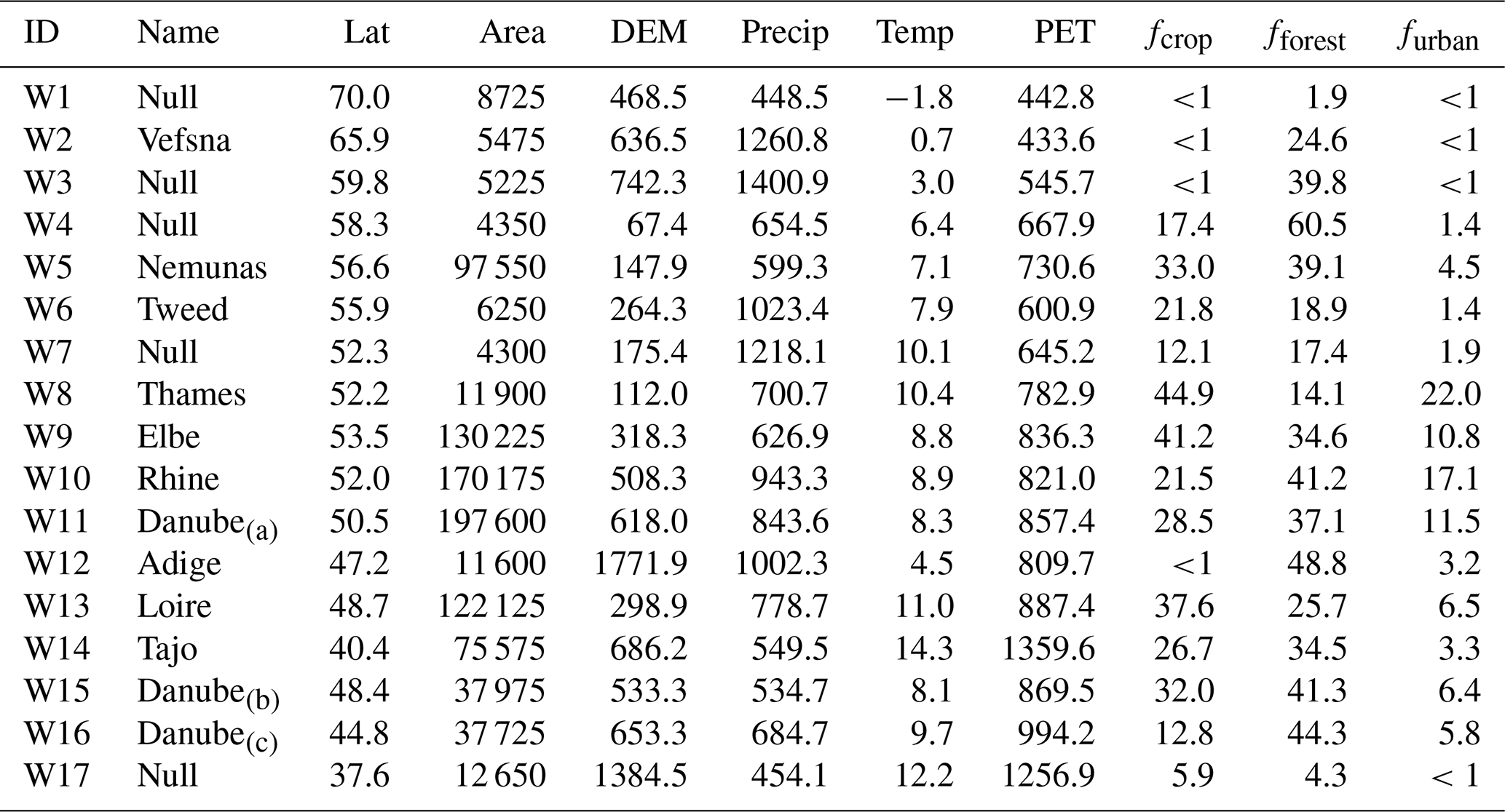
To ensure model generality, 17 catchments were selected for calibration and validation depending on the data availability (particularly stream stable water isotopes and nitrate), which span a wide range of characteristics in geography, climate, and anthropogenic managements (catchment locations, characteristics, and major hydrological and nitrogen inputs are shown in Fig. 2, Table 1, and Fig. S1, respectively). Anthropogenic management practices have a less dramatic effect than climate and geography in most catchments due to the relatively low proportion of urbanized areas. However, a few notable exceptions – such as the Rhine, Elbe, and Danube catchments – are included in the analysis, as these densely populated regions hold critical ecological, agricultural, and economic importance for Europe, and are subject to intensive human interventions in water management. This also provides a chance to examine the applicability of EcoTWIN in human-affected catchments.

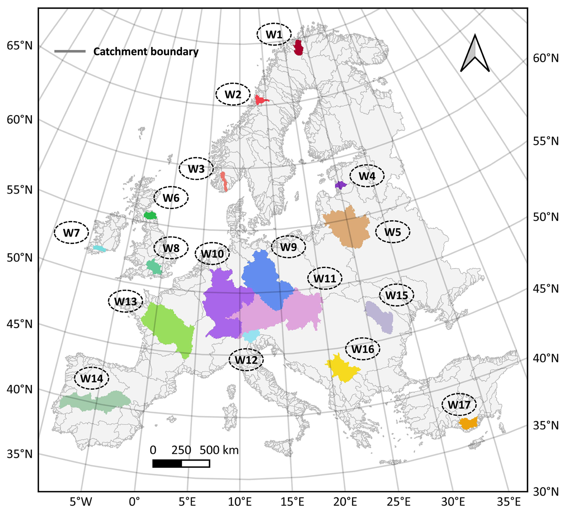
Figure 2 The selected catchments for model calibration and validation. The overview of key geographic, climatic, and nitrogen inputs are show in Fig. S1.

Table 1 Characteristics of the selected catchments. Lat depicts the latitude of upper left corner of the catchment. DEM and Area are the mean elevation in m.a.s.l. and catchment size in km². Precip, Temp, and PET are the annual averages of precipitation, air temperature, and potential evapotranspiration in mm yr⁻¹. f_crop, f_forest, and f_urban are the fractions of cropland, forest, and urbanized areas in 2019 in %. Null means no name is assigned for the catchment in the Catchment Characterisation and Modelling (CCM) database.

3.1 Model setup

EcoTWIN was setup for each of the 17 catchments for calibration with a spatial resolution of 5 km² and a temporal resolution of daily timesteps from 1980 to 2024 (with first two years for spin-up). As a fully distributed model, gridded GIS inputs are used in the model setup, including a digital elevation model, flow direction, slope, channel width, channel length, proportion of each land use type (Winkler et al., 2021), proportions of each soil type (world soil map, WRB2014), and soil properties (e.g., depth-dependent proportions of clay, sand, silt, and organic matter from SOILGRIDS). All spatial inputs were acquired with finer resolution (50 m or above) and resampled to the resolution of this application (5 km).

The climatic variables used to drive EcoTWIN include precipitation, air temperature, potential evapotranspiration, relatively humidity, and a few variables that are optional required for the calculation of channel evaporation (air pressure, net radiation, and wind speed). These climatic variables are available from the reanalysis products ERA5 and E-OBS, while PET is calculated using FAO Penman-Monteith equation. For nitrogen simulations, additional inputs are needed including the fertilization map (Grizzetti et al., 2021) and nitrate concentration of rainfall (Zhu et al., 2025) as the boundary of nitrogen addition from agricultural activities and wet deposition.

3.2 Model calibration

3.2.1 Method

The calibration was conducted separately for each catchment to test the applicability of EcoTWIN under different geological and climatic contexts. Three commonly used variables for hydrological and water quality modelling (discharge, stream water isotope composition, and in-stream NO₃–N concentrations) are employed for calibration. Their long-term time series were acquired at daily steps from different sources (discharge from GRDC, isotopes from Wateriso and GNIR, and NO₃–N concentration from global water quality database, GEMStat), and then compared with simulation results at multiple sites for each catchment. Here ¹⁸O was selected for isotopic validation due to its higher precision and data abundance. Given the discrepancy in duration of observations (especially for isotopes and NO₃–N), a separate calibration and validation based on a split-sample approach is difficult. Therefore, the full timescale (1982–2024) was used for calibration (and the validation introduced in Sect. 3.3).

The DiffeRential Evolution Adaptive Metropolis algorithm (DREAM) was selected for parameter optimisation due to its relatively efficient and effective performance for high-dimensional problems (as benchmarked in Wu et al., 2025c). The algorithm was implemented separately for each catchment with the same prior distribution of parameters (Table S1). The maximum iteration was set as 100 000 for each catchment (20 chains with maximum chain length of 5000), from which 40 best simulations were selected from the posterior distribution. The Kling-Gupta efficiency (KGE) statistic was used to construct an informal likelihood function for DREAM optimisation.

$$\begin{array}{}\text{(37)}& l={\left[\sum _{i=\mathrm{1}}^{N_{\mathrm{obs}}}\sum _{j=\mathrm{1}}^{N_{\mathrm{site}}}\left(\mathrm{1}-\mathrm{KGE}\right)\cdot w_{i,j}\right]}^{-m}\end{array}$$

Where l is the likelihood; N_obs and N_site are the number of observation types (discharge, isotopes, and nitrate) and sites. The weight w_i,j, defined for observation type i at site j, is assigned equally across sites such that the total weight for each observation type sums to $\mathrm{1}/\mathrm{3}$. m is an exponentially coefficient to stretch the likelihood surface that is often set based on the number of observation points. After prior test run, m was set as 500. Finally, the likelihood function is transformed to logarithmic form for numeric stability. The calibration was validated using Kling-Gupta efficiency (KGE), Root Mean Square Error (RMSE), Pearson Correlation Coefficient (Coefficient), and Percent bias (Pbias) (Table 2).

3.2.2 Calibration performance

EcoTWIN successfully reproduced the observed discharge in all 17 catchments with KGE exceeding 0.5 at most site (Fig. 3A and D; Table 2). Such performance is comparable to or better than previous continental calibration of hydrological models (e.g., ParFlow, Naz et al., 2023; E-HYPE, Donnelly et al., 2016).

Similarly, isotopic simulations also produced acceptable performances at most sites (Fig. 3B; Table 2). However, there are a few exceptions. The failure of isotopic simulations was found at two sites within the Alps region. This can be attributed to the uncertainty in precipitation isotopes and snowmelt isotopes (due to the lack of snowmelt elution fractionation; Ala-aho et al., 2017), the incorrect isotopic composition in groundwater, or the reduced applicability of degree-day model for mountainous areas in Europe. Such simulation deviation due to the uncertainty in data and boundary initialisation is often reported in previous calibration (Smith et al., 2021).

As for nitrogen simulation (Fig. 3C), the model produces comparable performances to existing nitrogen modelling at catchment (Wu et al., 2022, 2025b; Yang et al., 2018) and continental scales (Jones et al., 2023; Mikayilov et al., 2015). The degraded nitrogen simulations were found coarsely across Europe, but they are mostly in rivers/stream with low NO₃–N concentrations given the low RMSE in Table 2. Such low average values can easily trigger the degradation in KGE as one of the sub-components of KGE is highly sensitive to the mean deviation, though the absolute deviation remained low. Overall, we concluded that EcoTWIN has good capacity to reproduce in-stream components for a wide range of catchments and for relatively long periods.

Table 2 Calibration statistics for discharge (q), in-stream isotope (iso), and in-stream NO₃–N (no3) across the 17 selected catchments. Evaluation metrics represent the mean values computed within each catchment.

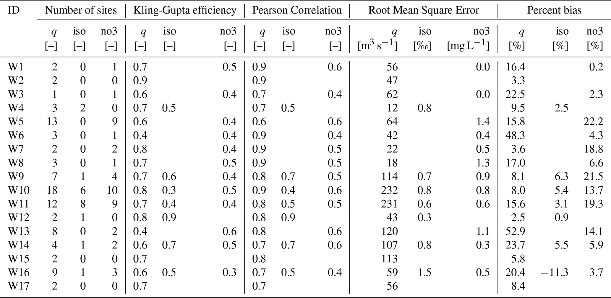
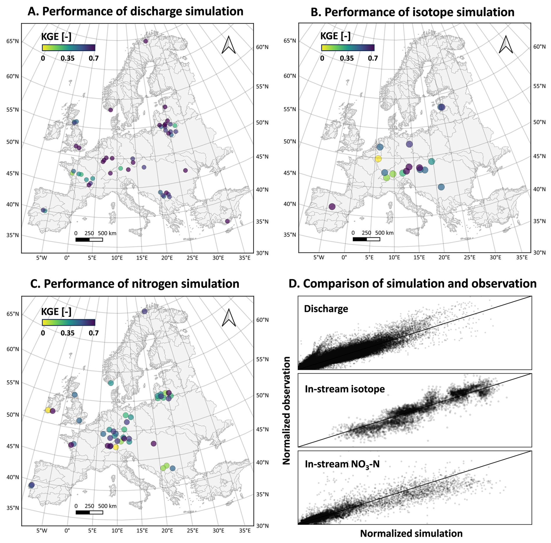
Figure 3 The simulation performance of discharge (A), in-stream isotope (B), and in-stream NO₃–N (C) evaluated using KGE. The comparison between simulation and observation values are shown in Panel (D). Catchment-specific performances are summarised in KGE, RMSE, Pearson correlation coefficient, and Pbias in Table 2.

3.3 Model validation

3.3.1 Method

Remote sensing or reanalysis products were further employed to validate uncalibrated internal model states or fluxes from three important perspectives in ecohydrological modelling – snow depth from ERA5, evapotranspiration from MODIS, and surface water mass anomaly from GRACE (as a storage proxy). The simulated variables corresponding to these products are, respectively, the depth of snow pack, the sum of soil evaporation, channel evaporation, and transpiration from all soil layers, and the anomaly of total water storage above groundwater (i.e., the sum of canopy storage, snow, soil water storages, and unsaturated storage). The validation was realised via resampling the remote sensing products to 5 km and comparing grid-to-grid with the modelled outputs. r² was used as the performance metrics, as KGE is not applicable for time series with zero average, yet the average of surface mass anomaly is close to 0.

Note that all three products may contain considerable uncertainties. ERA5 is a reanalysis product that combines historical observations into global estimates using modelling and data assimilation approaches, therefore inevitably embeds uncertainties associated with model structure and observational coverage (Hersbach et al., 2020). MODIS evapotranspiration is derived from remotely sensed spectral information, energy partitioning approaches and the Penman–Monteith framework, whose uncertainty may exceed 30 % depending on spatial scale and environmental conditions (Mu et al., 2011). GRACE infers changes in terrestrially stored water masses from spatial and temporal variations in the Earth's gravity field; however, its coarse spatial resolution can introduce substantial uncertainty when used for hydrological validation, particularly at basin or sub-basin scales (Tapley et al., 2004). Nevertheless, good agreement between simulations and remote sensing or reanalysis products can enhance confidence in the robustness of simulated spatial and temporal patterns, although it does not necessarily imply accurate representation of absolute magnitudes.

3.3.2 Validation performance

First, we compared the sum of soil evaporation, channel evaporation, and transpiration to MODIS evapotranspiration in each grid cell. The results in Fig. S2 and Table 3 shows a general good fit between simulation and MODIS records with coefficient of determination (R²) above 0.5 in most selected catchments. This is further validated after zooming into two representative catchments (W5 Nemunas and W10 Rhine) in Fig. 4A–B, where KGE reaches above 0.5 in >80 % of the catchment domain. The other evaluation metrics (RMSE, Pearson coefficient, RMSE, and percent bias shown in Table 3) also demonstrated the good performance of evapotranspiration simulations.

Then, the surface water mass anomaly from GRACE was compared to the anomaly of simulated surface storage, i.e., the sum of canopy storage, snow, soil water storages, and unsaturated storage. The grid-to-grid comparison in Fig. 4C–D shows an acceptable fit with R² above 0.3 in around half regions in catchment Nemunas (W5) and Rhine (W10), as well as other European catchments (Fig. S3 and Table 3). However, more degradation in performance was found compared to evapotranspiration simulation. For instance, the validation in Rhine shows degraded water storage simulation in Alpine regions. This is likely due to the locally complex topography and the simplified representation of snow accumulation and melt processes in the model, which struggle to capture the high spatial variability of storage in mountainous terrain. Besides, we also found degraded performance in coastal regions. For example, GRACE exhibited considerably increasing trends in water storage between 2005 to 2015 in two Nordic catchments (W2 and W3; Fig. S3), yet our simulations only showed a moderate increasing trend. Similar degraded performance was found in the coastal catchments (e.g., three British catchments W6–8 in UK; Fig. S3), though the magnitudes of simulation and GRACE data fit well. This is possibly attributed to the coarse resolution of GRACE which additionally considered the storage mass from ocean in coastal region yet not included in this terrestrial-explicit modelling.

Finally, the simulated snow depth was compared to the daily snow depth in ERA5 reanalysis products (ERA5 post-processed daily statistics on single levels; https://doi.org/10.24381/cds.4991cf48, Copernicus Climate Change Service, Climate Data Store, 2024). Results in Fig. 4E–F show a generally good agreement between simulations and ERA5 records with R²>0.5 in most regions in Nemunas and Rhine. Though degradation was found in a few other catchments (e.g., W14–17 in Fig. S4), these catchments generally experienced limited snow accumulation. In the other words, the absolute deviation was relatively limited for snow depth simulation demonstrated by low RMSE in Table 3.

Table 3 Validation performance of evapotranspiration (against MODIS records), water storage anomaly (against GRACE records), and snow depth (against ERA5 records). Performance is evaluated using the mean Kling–Gupta efficiency (KGE), Pearson correlation coefficient (r), root mean square error (RMSE), and percent bias (Pbias) across all grid cells within each of the 17 catchments.

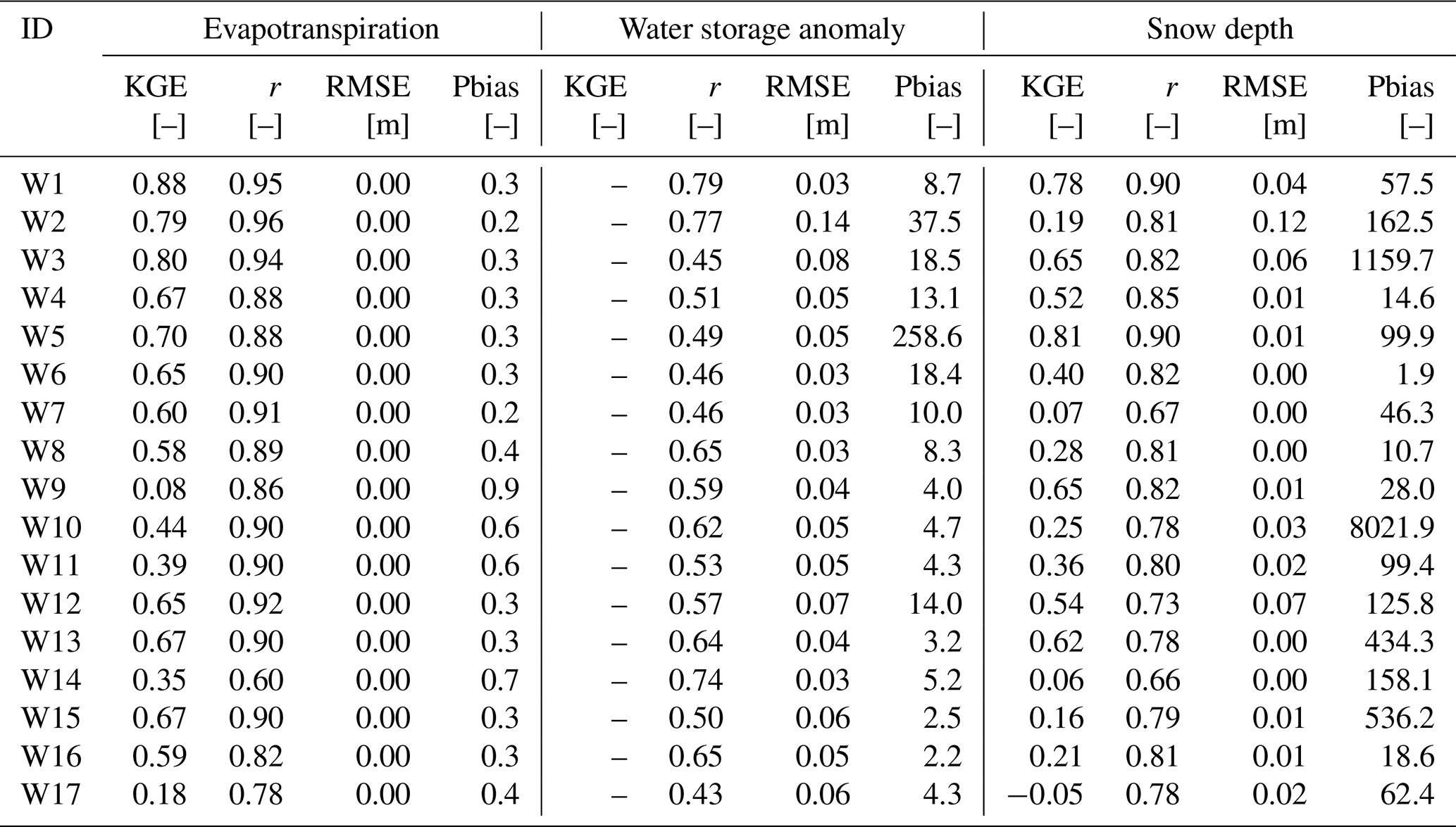
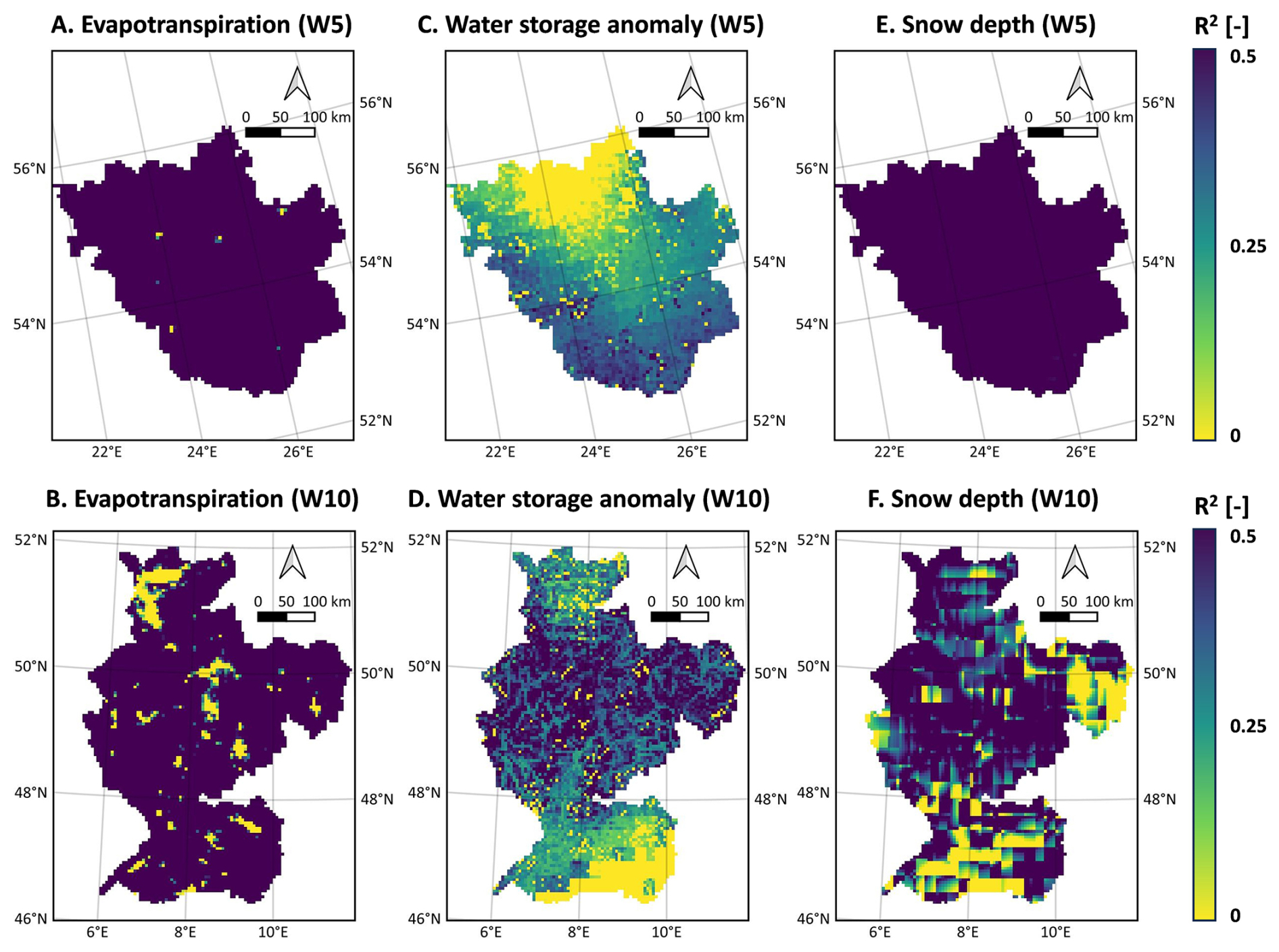
Figure 4 The grid-to-grid comparison (in coefficient of determination R²) between time series of simulated internal states/fluxes and the corresponding records extracted from remote sensing/reanalysis products, including evapotranspiration from MODIS (A–B), surface water mass anomaly from GRACE (C–D), and snow depth from ERA5 (E–F). The validation of two representative catchments is shown here (W5 Nemunas and W10 Rhine), while the spatial maps of all catchments were shown in Figs. S2–S4. The evaluation metrics in each catchment were summarised in Table 3.

4 Water age simulation and its link to water quality

Like many existing distributed hydrological and water quality models (e.g., SWAT, mHM, EcH₂O-iso, HYPE etc.), EcoTWIN can provide estimation of the main ecohydrological fluxes at high spatial and temporal resolutions, including canopy interception, snow melt-accumulation, infiltration, percolation through soil layers, groundwater recharge, and lateral flux routing at different horizontal phrases. Among these variables, a unique trait of EcoTWIN lies in its capacity to track water fluxes via isotopes, thus being able to provide a consistent estimate of water age and travel times. Therefore, in Fig. 5, these variables are shown as the long-term average from 1982 to 2024 for soil profile and stream water in Nemunas (W5) and Rhine (W10).

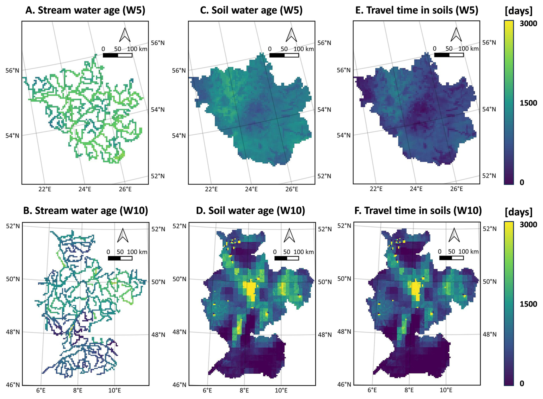
Figure 5 The simulated long-term average (1982–2024) of stream water age (A–B), soil water age (C–D), and travel time of soil water (E–F). Water age represents the time since water enters the catchments as precipitation, while travel time depicts the residence time of water within the specific storage (i.e., the soil profile in this figure). The spatial maps of all catchments are shown in Figs. S5–S7.

Generally, the magnitudes of water ages follow the geographic and climatic gradients, with younger water found in catchments with higher annual precipitation inputs. Those regions locate in Alpine regions – for instance around Alps in Southern Rhine, and in catchment W12 and W17 (Figs. S6–S7). The north-west coast of Europe (Fig. S5) also exhibited young water age, where lower temperature and net radiation limit the level of potential evapotranspiration, leading to larger percolation to deeper soil layers and groundwater. Such high turnover rates of water in these catchments (W2, W3, W6, and W7) are reflected by short travel time in soil profile with average values remaining below 500 d (Table 4).

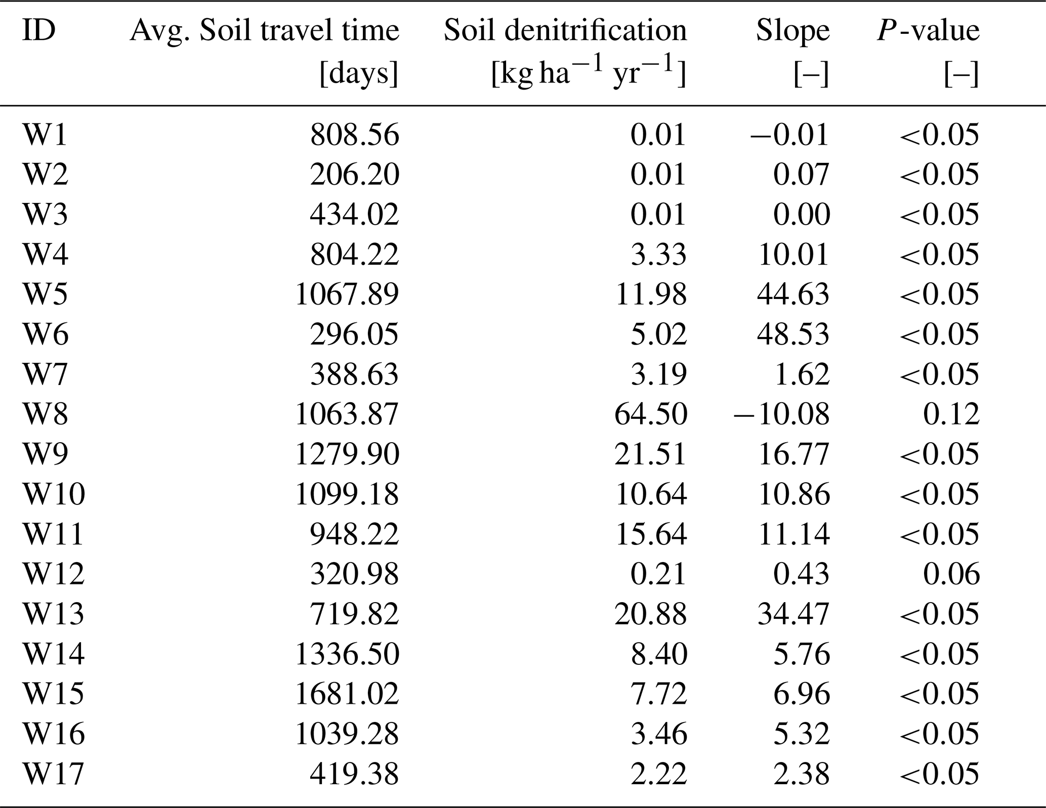
Table 4 Mean soil travel time and soil denitrification in selected catchments during 1982–2024. The regression slope of the fitted relationship between soil travel time and denitrification, along with the P-values of the Spearman test, are also reported.

A similar pattern was also found in mountainous regions with higher precipitation and lower potential evapotranspiration compared to lowland areas. Two clear examples are W12 and W17 located in the Alps and the Taurus Mountains where water ages and travel time remained below 500 d (Table 4 and Figs. S5–S7). In specific wet periods, the soil water ages and travel time can be reduced to just days, suggesting the rapid response of saturated hydrological systems. In contrast, the lowlands in central-west Europe showed much slower turnover rates. A typical example is Rhine (Fig. 5), where mean water ages reached up to 10 years in lowlands. Such phenomenon was also found in other European catchment (e.g., W9 Elbe, and W11 Danube).

Note that though water ages and travel time share similar magnitudes and spatial patterns. It is partly attributed to the fact that the travel time in the conceptualised storages increases exponentially in a sequential order. Taking the Rhine as an example, the average travel time in top soil layer, median soil layer, deep soil layer are 65, 225, 1291 d, respectively. Such a depth-dependence profile makes the overall ages/travel time follow the magnitude of bottom layer and leads to similarity between water ages and travel time. However, large discrepancies are possible between the two indices if a shallow lower boundary is adopted.

The estimation of travel time and water ages further provides opportunities to link hydrology and water quality processes in the modelling framework. The simplest and most intuitive way is to compare travel times and simulated biogeochemical process kinetics. Taking denitrification as an example, we applied linear regression and Spearman's correlation test to investigate the potential correlation between travel time of soil water and denitrification rates. The results in Table 4 showed the strong positive correlations in most agricultural-dominated catchments (W5, W6, W9, W10, W11, and W13) yet only weak or no positive correlation in remaining pristine watersheds. This suggests that travel time might be a key control on soil nitrogen removal in European croplands.

More insights can be gained via examination of the Damköhler Number, which quantifies the ratio between timescales of solute transport and biogeochemical transformation. Here in our modelling framework, it can be calculated as the ratio between the travel time of soil water and the time for all soil NO₃–N storage to be removed under the simulated denitrification rates. Damköhler numbers <1 mean that soil water nitrogen cannot be effectively removed during time of residence, indicating the dominance of transport over removal processes and the potential of nitrogen leaching. As shown in Fig. 6E–F, the long-term averages of Damköhler number remain below 1 in most croplands in Nemunas, Rhine, and other European catchments (Figs. 6 and S8), supporting the conclusion from the linear regression in Table 4 that travel time is a major limiting factor on soil nitrogen removal. Via the spatial- and temporal-explicit estimation of Damköhler number, EcoTWIN provides the opportunity to bridge the catchment hydrological and water quality with travel time.

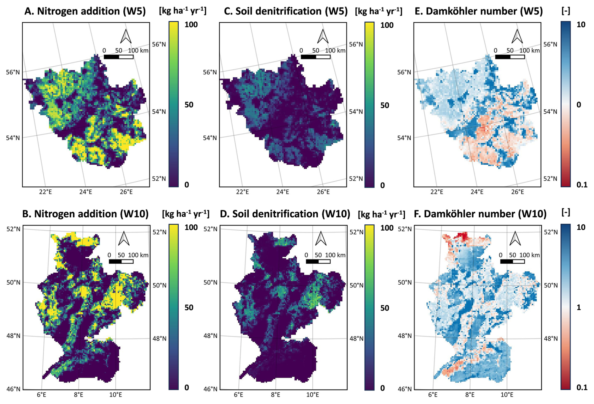
Figure 6 The simulated long-term average (1982–2024) of nitrogen addition from fertilization (A–B), soil denitrification (C–D), and Damköhler number (E–F). Note that logarithmic scale is used for Damköhler number. The spatial map containing Damköhler number in all catchments is shown in Fig. S8.

5 Discussion

5.1 Structural and Functional Merits of EcoTWIN

As a new tracer-aided ecohydrological model, EcoTWIN has novel advantages compared to previous models. In this section, we briefly introduced the merits in model structure, applicability, and insights from tracer-aided simulation.

5.1.1 Integrated C$++$ framework

Applications of large-scale modelling have been increasingly popular due to the accelerating development of observation networks and availability of remote sensed data. However, it severely increases the computational burden of ecohydrological modelling. Especially for fully distributed models, increasing size of the model domain can lead to exponential increase in computation demands. In this context, an integrated framework in C$++$ can significantly accelerate the modelling tasks, as all computation can be conducted within memory thereby avoiding the additional input/output overhead associated with disk-based operations in loosely coupled model chains (e.g., EcH₂O-iso-nitrate; Yang et al., 2024). A standard test was not performed, but based on our modelling experience in the same catchment with different models, the speed of EcoTWIN (∼ 5 s for a simulation with 285 grid cells and 30 years at daily timestep) is close to the water quality model mHM-Nitrate (∼ 5 s yet without isotopic simulations; Wu et al., 2022) and easily outperforms EcH₂O-iso-nitrate (7 min; Wu et al., 2025b).

5.1.2 Selective disassembly structure

EcoTWIN incorporates a wide range of ecohydrological processes from canopy to groundwater, which not only include natural processes but also anthropogenic activities like irrigation. Land managements can also be represented by dynamic parametrisation, thus enabling EcoTWIN to function as a learning tool to investigate the impacts of changes in anthropogenic management over natural ecosystems; for instance, the land use distribution was updated every 10 years in our test examples to reflect the moderate increases in afforestation in the past 45 years in Europe. More importantly, unlike hard coded process representations/equations in most ecohydrological models, EcoTWIN has a selective disassembly structure, which provides alterative conceptualisations for several important hydrological processes (canopy interception, percolation, groundwater recharge, as well as three pedotransfer functions for initialising soil properties). Modellers can benefit from such flexible model structures by either selecting process representations best suited to field knowledge or data prior to calibration, or integrating module selection into the calibration thus enabling simultaneous optimisation of model structure and corresponding parameters. The latter aspect, i.e., the optimisation of model structure, can be realised together with the recently developed optimisation algorithm DREAM_(LOAX) that aims to identify the deficits in model structure during calibration (Wu et al., 2025a).

5.1.3 Transferability to contrasting geographic and climatic contexts

To thoroughly test the applicability of EcoTWIN, 17 catchments with different climatic and geographical contexts were selected for calibration and validation, spanning over most biomes in Europe, from snow-dominated watersheds in Nordic or alpine regions, to agricultural-influenced lowlands catchments, and Mediterranean ecosystems (Fig. 2 and Table 1). Through multi-criteria calibration against three objectives at multiple sites, the model successfully reproduced the seasonality and peaks of discharge, in-stream isotopes, and NO₃–N concentrations in most catchments. Such performance is comparable or better than the previous model benchmarks at similar scales (Bajracharya et al., 2023; Mikayilov et al., 2015; Rakovec et al., 2016, 2019). Note that the concentration of NO₃–N was used for calibration, whose accurate simulation is more difficult than NO₃–N loads given the naturally good performance in discharge. In the other words, hydrological simulation is often the least problematic part in integrated water quality modelling, as it is mostly dominated by natural catchment properties while nitrogen cycling is more interfered by anthropogenic managements (e.g., fertilization and irrigation) (Wu et al., 2025b). Additionally, the simulated internal fluxes were also compared to three reanalysis products in hydrological simulations, corresponding to the key fluxes or storage states in hydrological cycling (snow melt-accumulation, evapotranspiration, and water storage). The results show that constrained by isotopes, EcoTWIN was able to reproduce comparable hydrological modelling results to the remote sensing data without direct calibration regarding magnitudes, spatial patterns, and temporal dynamics. The only degraded performance was found in GRACE surface mass anomaly in coastal regions. There are two potential reasons: (i) the coarse resolution of GRACE might account for mass shifts in both ocean and land, yet EcoTWIN only produces mass anomaly in terrestrial systems; (ii) bidirectional fluxes across the land-ocean interface might drive key changes in coastal systems, which is not considered in current version of EcoTWIN. Nonetheless, given the relatively good agreement with most available data, we conclude that EcoTWIN is applicable across a range of terrestrial ecosystems from boreal to temperate and subtropical climate.

5.1.4 Bridging hydrology and water quality with water ages

Further to the inference of hydrological and nitrogen processes that is also available in other distributed water quality models (Wellen et al., 2015), a unique trait of EcoTWIN lies in its capacity to track water fluxes and ages with stable water isotopes. As a tracer-aided model, EcoTWIN not only simulates the celerity of catchment response, but tracks the velocity of water via different flow paths. The importance of delineating flow paths within catchments has long been recognized by hydrologists, and has motivated the development of many indices to describe the movement of water molecule at catchment-scale and estimate associated timescales (Sprenger et al., 2019). A few examples are water ages, transient time distribution, and young water fractions (Benettin et al., 2015; Hrachowitz et al., 2013; Jasechko et al., 2016). However, those indices are mainly calculated in a lumped manner where different flow paths in the catchment are characterised as a black box, thus characterising the overall input-output dynamics yet potentially omitting important spatio-temporal variability of hydrological boundary conditions. Instead, EcoTWIN, benefiting from the gridded-based structure, can utilise the increasingly available spatial information (e.g., gridded remote sensing datasets) thus characterising the water ages and travel time in a spatially-explicit manner. Note that simulations of water age/travel time, like other ecohydrological processes, are sensitive to spatial resolution. The coarse resolution used for large catchments (e.g., 5 km in this study) may obscure the sub-grid heterogeneity. For instance, local hydrological hotspots characterized by short travel times and young water ages can be damped or averaged out at coarser resolutions, as reported in modelling studies using EcH₂O-iso (Smith et al., 2021; Yang et al., 2023b). However, this limitation can be mitigated by increasing spatial resolution, and it does not undermine the utility of EcoTWIN for water-tracking.

Compared to water age which quantifies the age of water within the overall system, travel time, accounting for the water age within a specific storage, is more important in understanding the links between hydrological and nutrient cycles. Such an index, also known as transit time or exposure time, forms one of the fundamental components of water quality modelling. Therefore, the travel time estimated by EcoTWIN has potential to improve the simulation of biogeochemical transformations in water quality models interfaced with simplified hydrological modules (e.g., MONERIS; Venohr et al., 2011). Moreover, travel time can be used as a proxy to bridge hydrological processes and biogeochemical transformations. Here we presented a simple framework to calculate the Damköhler Number for denitrification. By using the simulated travel time and reaction timescale (i.e., the time for full removal of nitrogen storage under current denitrification rates), estimation of Damköhler Number was achieved in a spatially- and temporally-explicit manner (Fig. 6E–F), which can highlight where and when soil nitrogen removal is constrained by the limited exposure time in the catchment. Such high-resolution information is unique, as the use of this index has been largely restricted to steady-state groundwater systems or riparian/hyporheic zones due to the difficulty in quantifying processing time and residence time at larger scales (Ocampo et al., 2006; Wu et al., 2022).

5.2 Limitations and roadmap for future development

Despite these advances, EcoTWIN has limitations. In this section, the uncertainties in model structure and conceptualisation are introduced, as well as the potential roadmaps for future developments.

5.2.1 Potential towards physics-based conceptualisation of groundwater

Groundwater in EcoTWIN is characterised as two conceptual storages linking with adjacent upstream and downstream storages following the topographic gradients. Such conceptualisation, although has been widely employed in hydrological models (e.g., SWAT, mHM, EcH₂O, STARR, etc.), does not align with the physical mechanisms of groundwater routing, as groundwater flow direction follows the hydraulic gradients which may not entirely coincide with topographic gradients (Condon et al., 2021). Such simplified routing has less effect in large catchments with clear topographic gradients (e.g., Rhine starting from Alps to North plain), yet might cause biased estimation in water mass balance for flatter headwater catchments (Yang et al., 2025). Therefore, we plan to further incorporate an additional groundwater module to realise physics-based routing following Darcy's Law in future.

5.2.2 Revisiting mixing strategies

Mixing strategy is a key component in water quality or tracer models describing the flux-storage behaviours along specific flow paths. There has long been a debate on different mixing assumptions and theories. A typical example is the two-water-world hypothesis, where water storage in the soil profile is differentiated into a tightly-bound pool and a mobile-water pool (McDonnell, 2014). Such conceptualisation is close to the definition of soil matrix flow and preferential flow: the existence of free-flowing preferential flow will bypass the soil matrix vertically and accelerate the lateral drainage via direct connection with channel network (Hrachowitz et al., 2013; Sprenger et al., 2019). However, a complete mixing strategy is often regarded as a reasonable first approximation in many situations and is used in most water quality and tracer models (Jung et al., 2025). This is not only attributed to its computational simplicity, but also the difficulty in conceptualising preferential flow in an evidenced-based manner. In the other words, even with the recognition of preferential flow, its calculation is often hindered by the subsurface heterogeneity in soils and bedrock; a good visualisation is given in Fig. 7 in Sprenger et al. (2019). Alternatively, partial mixing has been developed for ecohydrological models (e.g., Hrachowitz et al., 2013), which could be added as a complementary mixing strategy in EcoTWIN. However, as benchmarked in Hrachowitz et al. (2013), the partial mixing brings only moderate improvements in simulations yet can introduce challenges to model spin-up (the increasing instability of storage ages due to the exchange between bypass and storage compartment). Moreover, the realisation of partial mixing, like preferential flow, relies on additional parameters to describe the timing and extent of mixing thus introducing additional parametric uncertainty. Therefore, we recommend a rigorous evaluation of the necessity of partial mixing before any application.

5.2.3 Complementing the in-stream biogeochemical processes

Transformation is as crucial as transport in inland-water nitrogen cycling (Wang et al., 2024). In the current version of EcoTWIN, denitrification is the only in-stream process of nitrogen loss. However, recent studies have shown that other processes are involved which may be important for aquatic nitrogen cycling. An example originates from Wang et al. (2024), where global inland-water modelling shows that in-stream denitrification only accounts for a minor fraction of NO₃–N removal compared to biological uptake. Though their modelling considers lakes and reservoirs where primary production of benthic plants and algae is usually greater than that in rivers, in-stream assimilation might still play a significant role, particularly, in slow-flowing river systems. This is supported by a recent modelling study that estimated nitrogen retention at 15 min interval based on high-frequency NO₃–N data (Yang et al., 2023a). Therefore, we plan to further compliment EcoTWIN with in-stream assimilation conceptualisation, as well as other potentially important riverine processes (e.g., nitrogen burial in sediments; Akbarzadeh et al., 2019).

5.2.4 Integrated calibration framework to embrace equifinality

Strictly speaking, equifinality is not specifically linked to EcoTWIN, but remains a universal problem for calibration or parameter tunning for almost all ecohydrological models. It is reflected in multiple parameters sets yielding similarly good model performance, thus increasing the uncertainty in process inference. The extent of equifinality is primarily controlled by the magnitude of parameters and observation/objectives (Wu et al., 2025c). Unfortunately, conceptualisations across diverse process domains (e.g. for hydrology, isotopes and N-cycling) in EcoTWIN also lead to a relatively large number of parameters. Such risk in equifinality can be potentially constrained via sensitivity analysis, but can still remain an issue given the ubiquitous epistemic uncertainty in data and model structure (Beven, 2006, 2015). Alternatively, the recently developed calibration algorithm DREAM_(LoAX) provides an opportunity to embrace equifinality by tunning parameters based on the limits-of-acceptability theory under the equifinality thesis (Wu et al., 2025a). The integrated modelling framework of EcoTWIN and DREAM_(LoAX) can potentially increase the robustness of model calibration and inference.

6 Conclusions

Uncertainty is a central concern in ecohydrological modelling, as models are not only used for prediction of specific variables, but also for process inference (backtracking internal processes from available observations) that are inherently embedded within considerable uncertainty. Stable water isotopes can help effectively constrain hydrological fluxes due to their conservative nature, motivating the increased development of tracer-aided models. However, few attempts have been made to incorporate a tracer-aided hydrological framework into water quality models.

Therefore, we introduced EcoTWIN, a fully distributed tracer-aided ecohydrological model that tracks water, isotopic, and nutrient fluxes simultaneously in an integrated C$++$-based framework. To thoroughly validate the model, 17 large European catchments were selected with a wide range of geographic and climatic gradients (from snow-dominated watersheds in Nordic or alpine regions, to agricultural-influenced lowlands catchments, and Mediterranean ecosystems). The model was calibrated against long-term observations of discharge, in-stream isotopes, and NO₃–N concentrations during 1980–2024 in each of the 17 catchments. Additionally, uncalibrated internal states and fluxes were also compared with three remote sensing products (ERA5 snow depth, MODIS evapotranspiration, and GRACE surface water anomaly) to validate the credibility of process inference.

The generally good agreements in both calibrated in-stream components and uncalibrated internal flux-states demonstrated that EcoTWIN is a transferable, flexible prediction and learning tool for process inference across biomes ranging from boreal to subtropical climate. Constrained by tracer simulations, the model not only reproduces the celerity of hydrological systems, but also tracks the velocity. Water ages and travel time are embedded in EcoTWIN to provides spatio-temporal-explicit insights into when, where, and how water moves in the system. Such indices further provide the opportunities to efficiently bridge hydrology and water quality at large catchment-scales. An example was presented using the Damköhler Number to identify regions where denitrification was limited by fast turnover rates of water.

Following this “proof of concept” we also see numerous areas where future developments can improve the limitations in the 1.0 version of the model.